Embed Size (px)
Citation preview

1
A Comprehensive Evaluation of the Differential Geometry of
Cartan Connections with Metric Structure
By Daniel L. Indranu
Introduction
The splendid, profound, and highly intuitive interpretation of differential geometry by E. Cartan, which was first applied to Riemann spaces, has resulted in a highly systematic
description of a vast range of geometric and topological properties of differentiable manifolds. Although it possesses a somewhat abstract analytical foundation, to my
knowledge there is no instance where Riemann-Cartan geometry, cast in the language of
differential forms (i.e., exterior calculus), gives a description that is in conflict with the classical tensor analysis as formalized, e.g., by T. Levi-Civita. Given all its successes,
one might expect that any physical theory, which relies on the concept of a field, can be elegantly built on its rigorous foundation. Therefore, as long as the reality of metric
structure (i.e., metric compatibility) is assumed, it appears that a substantial modified
geometry is not needed to supersede Riemann-Cartan geometry.
A common overriding theme in both mathematics and theoretical physics is that of
unification. And as long as physics can be thought of as geometry, the geometric objects
within Riemann-Cartan geometry (such as curvature for gravity and torsion for intrinsic
spin) certainly help us visualize and conceptualize the essence of unity in physics. Because of its intrinsic unity and its breadth of numerous successful applications, it might
be possible for nearly all the laws governing physical phenomena to be combined and written down in compact form via the structural equations. By the intrinsic unity of
Riemann-Cartan geometry, I simply refer to its tight interlock between algebra, analysis,
group representation theory, and geometry. At least in mathematics alone, this is just as close as one can get to a “final” unified description of things. I believe that the unifying
power of this beautiful piece of mathematics extends further still.
I’m afraid the title I’ve given to this work has a somewhat narrow meaning, unlike the
way it sounds. In writing this article, my primary goal has been to present Riemann-
Cartan geometry in a somewhat simpler, more concise, and therefore more efficient form
than others dealing with the same subject have done before. I have therefore had to drop whatever mathematical elements or representations that might seem somewhat highly
counterintuitive at first. After all, not everyone, unless perhaps he or she is a
mathematician, is familiar with abstract concepts from algebra, analysis, and topology, just to name a few. Nor is he or she expected to understand these things. But one thing
remains essential, namely, one’s ability to catch at least a glimpse of the beauty of the presented subject via deep, often simple, real understanding of its basics. As a non-
mathematician (or simply a “dabbler” in pure mathematics), I do think that pure
mathematics as a whole has grown extraordinarily “strange”, if not complex (the weight of any complexity is really relative of course), with a myriad of seemingly separate
branches, each of which might only be understood at a certain level of depth by the pure mathematicians specializing in that particular branch themselves. As such, a comparable
2
complexity may also have occurred in the case of theoretical physics itself as it
necessarily feeds on the latest formalism of the relevant mathematics each time. Whatever may be the case, the real catch is in the essential understanding of the basics. I
believe simplicity alone will reveal it without necessarily having to diminish one’s perspectives at the same time. After all, this little work is intended for beginners.
1. A brief elementary introduction to the Cartan(-Hausdorff) manifold ∞C
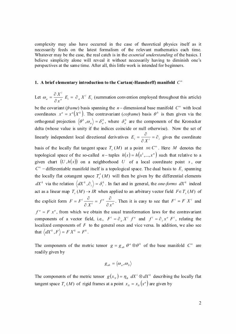
Let i
i
aia
i
a EXEx
X∂=
∂
∂=ω (summation convention employed throughout this article)
be the covariant (frame) basis spanning the −n dimensional base manifold ∞C with local
coordinates ( )kaa Xxx = . The contravariant (coframe) basis bθ is then given via the
orthogonal projection b
aa
b δωθ =, , where b
aδ are the components of the Kronecker
delta (whose value is unity if the indices coincide or null otherwise). Now the set of
linearly independent local directional derivatives iiiX
E ∂=∂
∂= gives the coordinate
basis of the locally flat tangent space )(MTx at a point ∞∈Cx . Here M denotes the
topological space of the so-called −n tuples ( ) ( )nxxhxh ...,,1= such that relative to a
given chart ( )( )xhU , on a neighborhood U of a local coordinate point x , our
−∞C differentiable manifold itself is a topological space. The dual basis to iE spanning
the locally flat cotangent space )(* MTx will then be given by the differential elements
kdX via the relation k
ii
kdX δ=∂, . In fact and in general, the one-forms kdX indeed
act as a linear map IRMTx →)( when applied to an arbitrary vector field )(MTF x∈ of
the explicit form a
a
i
i
xf
XFF
∂
∂=
∂
∂= . Then it is easy to see that
ii XFF = and
aa xFf = , from which we obtain the usual transformation laws for the contravariant
components of a vector field, i.e., ai
a
i fXF ∂= and ia
i
i Fxf ∂= , relating the
localized components of F to the general ones and vice versa. In addition, we also see
that kkk FXFFdX ==, .
The components of the metric tensor ba
abgg θθ ⊗= of the base manifold ∞C are
readily given by
baabg ωω ,=
The components of the metric tensor ( ) ki
ikN dXdXxg ⊗= η describing the locally flat
tangent space )(MTx of rigid frames at a point ( )aNN xxx = are given by
3
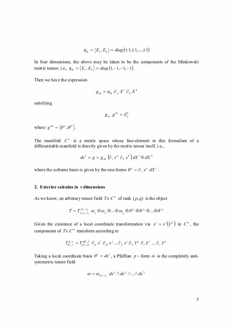
( )1,...,1,1, ±±±== diagEE kiikη
In four dimensions, the above may be taken to be the components of the Minkowski
metric tensor, i.e., ( )1,1,1,1, −−−== diagEE kiikη .
Then we have the expression
k
b
i
aikab XXg ∂∂= η
satisfying
b
a
bc
ac gg δ=
where baabg θθ ,= .
The manifold ∞C is a metric space whose line-element in this formalism of a
differentiable manifold is directly given by the metric tensor itself, i.e.,
( ) kib
k
a
iab dXdXxxggds ⊗∂∂==2
where the coframe basis is given by the one-forms ia
i
a dXx∂=θ .
2. Exterior calculus in n dimensions
As we know, an arbitrary tensor field ∞∈CT of rank ),( qp is the object
p
q
q
p
jjj
iii
iii
jjjTT θθθωωω ⊗⊗⊗⊗⊗⊗⊗= ...... 21
21
21
21
...
...
Given the existence of a local coordinate transformation via ( )αxxx ii = in ∞C , the
components of ∞∈CT transform according to
ηνµ
λβαλαβ
ηµν xxxxxxTT rlk
sjisij
rkl ∂∂∂∂∂∂= .........
...
...
...
Taking a local coordinate basis ii dx=θ , a Pfaffian −p form ω is the completely anti-
symmetric tensor field
p
p
iii
iii dxdxdx /\.../\/\ 21
21 ...ωω =

4
where
pp
p
p jjjiii
jjj
iii dxdxdxp
dxdxdx ⊗⊗⊗≡ ...!
1/\.../\/\ 2121
21
21...
...δ
In the above, the p
p
iii
jjj
...
...21
21δ are the components of the generalized Kronecker delta. They
are given by
=∈∈=
p
ppp
p
p
p
p
p
p
i
j
i
j
i
j
i
j
i
j
i
j
i
j
i
j
i
j
ii
jjj
iii
jjj
δδδ
δδδ
δδδ
δ
...
............
...
...
det
21
2
2
2
1
2
1
2
1
1
1
1
21
21
21
...
...
...
...
where ( )pp jjjjjj g ...... 2121
det ε=∈ and ( )
pp iiiiii
g
...... 2121
det
1ε=∈ are the covariant and
contravariant components of the completely anti-symmetric Levi-Civita permutation
tensor, respectively, with the ordinary permutation symbols being given as usual by
qjjj ...21ε and piii ...21ε .
We can now write
p
p
p
p
jjj
iii
iii
jjj dxdxdxp
/\.../\/\!
121
21
21
21 ...
...
... ωδω =
such that for a null −p form 0=ω its components satisfy the relation
0...
...
... 21
21
21=
p
p
p iii
iii
jjj ωδ .
By meticulously moving the idx from one position to another, we see that
pqp
qpp
ijjjiiip
jjjiiii
dxdxdxdxdxdxdx
dxdxdxdxdxdxdx
/\/\.../\/\/\/\.../\/\)1(
/\.../\/\/\/\/\.../\/\
21121
21121
−
−
−=
and
pq
qp
iiijjjpq
jjjiii
dxdxdxdxdxdx
dxdxdxdxdxdx
/\.../\/\/\/\.../\/\)1(
/\.../\/\/\/\.../\/\
2121
2121
−=
Let ω and π be a −p form and a −q form, respectively. Then, in general, we have the
following relations:

5
( )( ) ( ) πωπωπω
πωπω
πωωππω
ddd
ddd
dxdxdxdxdxdx
p
jjjpii
jjjiii
pq q
qp
/\1/\/\
/\.../\/\/\/\.../\/\/\)1(/\ 2121
2121 ......
−+=
+=+
=−=
Note that the mapping ωω dd =: is a ( )−+1p form. Explicitly, we have
121
1
2121
21/\/\.../\/\
)!1(
)1( ......
...
+
+∂
∂
+−
= pp
p
pp
p
ijjj
i
iiiiii
jjj
p
dxdxdxdxxp
dω
δω
For instance, given a (continuous) function f , the one-form i
i dxfdf ∂= satisfies
0/\2 =∂∂=≡ ik
ik dxdxfddffd . Likewise, for the one-form i
i dxAA = , we have ik
ik dxdxAdA /\∂= and therefore 0/\/\2 =∂∂= ikl
ikl dxdxdxAAd , i.e.,
0=∂∂ ikl
ikl
rst Aδ or 0=∂∂+∂∂+∂∂ klilikikl AAA . Obviously, the last result holds
for arbitrary −p forms sij
rkl
...
...Π , i.e.,
0...
...
2 =Π sij
rkld
Let us now consider a simple two-dimensional case. From the transformation law
αα xdxdx ii ∂= , we have, upon employing a positive definite Jacobian, i.e.,
( )( ) 0
,
,>
∂
∂βα xx
xxji
, the following:
( )( )
βαβα
βαβα xdxd
xx
xxxdxdxxdxdx
jijiji
/\,
,
2
1/\/\
∂
∂=∂∂=
It is easy to see that
( )( )
21
21
2121
/\,
,/\ xdxd
xx
xxdxdx
∂
∂=
which gives the correct transformation law of a surface element.
We can now elaborate on the so-called Stokes theorem. Given an arbitrary function f ,
the integration in a domain D in the manifold ∞
C is such that
( ) ( )( ) ( )( )
21
21
2121
,
,/\ xdxd
xx
xxxxfdxdxxf
D D
ii∫∫ ∫∫ ∂
∂= α
6
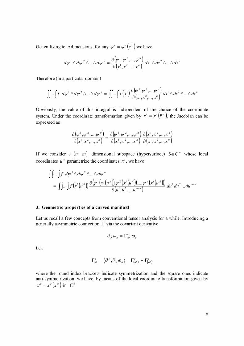
Generalizing to n dimensions, for any ( )kii xψψ = we have
( )( )
n
n
nn
dxdxdxxxx
ddd /\.../\/\...,,,
...,,,/\.../\/\
21
21
2121
∂
∂=
ψψψψψψ
Therefore (in a particular domain)
( ) ( )( )
n
n
nin
dxdxdxxxx
xfdddf /\.../\/\,...,,
,...,,.../\.../\/\...
21
21
2121∫ ∫∫∫∫∫ ∂
∂=
ψψψψψψ
Obviously, the value of this integral is independent of the choice of the coordinate
system. Under the coordinate transformation given by ( )αxxx ii = , the Jacobian can be
expressed as
( )( )
( )( )
( )( )n
n
n
n
n
n
xxx
xxx
xxxxxx ,...,,
,,...,
,...,,
,...,,
,...,,
...,,,21
21
21
21
21
21
∂
∂
∂
∂=
∂
∂ ψψψψψψ
If we consider a ( )−−mn dimensional subspace (hypersurface) ∞∈CS whose local
coordinates Au parametrize the coordinates ix , we have
( )( ) ( )( ) ( )( ) ( )( )( )( )
mn
mn
AinAiAiAi
n
dududuuuu
uxuxuxuxf
dddf
−−∫ ∫∫
∫ ∫ ∫
∂∂
= ...,...,,
,...,,...
/\.../\/\...
21
21
21
21
ψψψ
ψψψ
3. Geometric properties of a curved manifold
Let us recall a few concepts from conventional tensor analysis for a while. Introducing a
generally asymmetric connection Γ via the covariant derivative
c
c
abab ωω Γ=∂
i.e.,
( ) [ ]c
ab
c
abab
cc
ab Γ+Γ=∂=Γ ωθ ,
where the round index brackets indicate symmetrization and the square ones indicate anti-symmetrization, we have, by means of the local coordinate transformation given by
( )αxxx aa = in ∞C
7
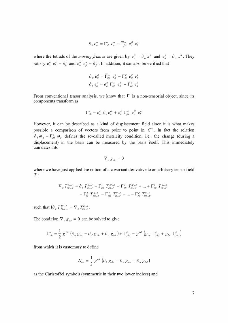
λβαβλ
ααbac
c
abab eeee Γ−Γ=∂
where the tetrads of the moving frames are given by αα xe aa ∂= and aa xe αα ∂= . They
satisfy a
bb
a ee δαα = and α
ββα δ=a
a ee . In addition, it can also be verified that
ca
cbb
aa
b
cba
bc
aa
eeee
eeee
αβλ
αβλα
βαλλ
αβαβ
Γ−Γ=∂
Γ−Γ=∂
From conventional tensor analysis, we know that Γ is a non-tensorial object, since its components transform as
λβα
βλαα
α ba
c
ab
cc
ab eeeee Γ+∂=Γ
However, it can be described as a kind of displacement field since it is what makes
possible a comparison of vectors from point to point in ∞C . In fact the relation
c
c
abab ωω Γ=∂ defines the so-called metricity condition, i.e., the change (during a
displacement) in the basis can be measured by the basis itself. This immediately translates into
0=∇ abc g
where we have just applied the notion of a covariant derivative to an arbitrary tensor field
T :
sij
plm
p
rk
sij
rlp
p
mk
sij
rpm
p
lk
pij
rlm
s
pk
sip
rlm
j
pk
spj
rlm
i
pk
sij
rlmk
sij
rlmk
TTT
TTTTT
...
...
...
...
...
...
...
...
...
...
...
...
...
...
...
....
...
...
Γ−−Γ−Γ−
Γ++Γ+Γ+∂=∇
such that ( ) sij
rlmk
sij
rlmk TT ...
...
...
...∇=∂ .
The condition 0=∇ abc g can be solved to give
( ) [ ] [ ] [ ]( )e
dabe
e
dbae
cdc
abbdaabddab
cdc
ab ggggggg Γ+Γ−Γ+∂+∂−∂=Γ2
1
from which it is customary to define
( )bdaabddab
cdc
ab gggg ∂+∂−∂=∆2
1
as the Christoffel symbols (symmetric in their two lower indices) and

8
[ ] [ ] [ ]( )e
dabe
e
dbae
cdc
ab
c
ab gggK Γ+Γ−Γ=
as the components of the so-called contorsion tensor (anti-symmetric in the first two mixed indices).
Note that the components of the torsion tensor are given by
[ ] ( )αβ
βαβ
βααα bccbcbbc
aa
bc eeeee Γ−Γ+∂−∂=Γ2
1
where we have set λαβλ
αβ cc eΓ≡Γ .
The components of the curvature tensor R of ∞C are then given via the relation
( )
[ ]sab
rcdw
w
pq
s
wpq
wab
rcd
b
wpq
saw
rcd
a
wpq
swb
rcd
w
rpq
sab
wcd
w
dpq
sab
rcw
w
cpq
sab
rwd
sab
rcdqppq
T
RTRTRT
RTRTRTT
...
...
...
...
...
...
...
...
...
...
...
...
...
...
...
...
2
...
...
∇Γ−
−−−−
+++=∇∇−∇∇
where
( ) d
ec
e
ab
d
eb
e
ac
d
abc
d
acb
d
abc
d
ec
e
ab
d
eb
e
ac
d
abc
d
acb
d
abc
KKKKKKB
R
−+∇−∇+∆=
ΓΓ−ΓΓ+Γ∂−Γ∂=
ˆˆ
where ∇ denotes covariant differentiation with respect to the Christoffel symbols alone, and where
( ) d
ec
e
ab
d
eb
e
ac
d
abc
d
acb
d
abcB ∆∆−∆∆+∆∂−∆∂=∆
are the components of the Riemann-Christoffel curvature tensor of ∞C .
From the components of the curvature tensor, namely, d
abcR , we have (using the metric
tensor to raise and lower indices)
( ) [ ] [ ] [ ]
( ) [ ] [ ] [ ] [ ]c
ad
d
cb
abacb
abc
d
cd
b
ab
acc
bca
aba
a
c
ad
d
cb
d
cd
c
ab
c
acb
d
cb
c
ad
c
abcab
c
acbab
gKKggBRR
KKKKBRR
ΓΓ+−ΓΓ−Γ∇−∆=≡
ΓΓ+Γ+Γ∇−−∇+∆=≡
2ˆ2
2ˆˆ
where ( ) ( )∆≡∆ c
acbab BB are the components of the symmetric Ricci tensor and
( ) ( )∆≡∆ a
aBB is the Ricci scalar. Note that d
bcadabc KgK ≡ and a
de
becdacb KggK ≡ .

9
Now since
( )( )( )( ) [ ]
b
aba
b
ab
a
b
ab
b
ba
b
ba
g
g
Γ+∂=Γ
∂=∆=∆=Γ
2detln
detln
we see that for a continuous metric determinant, the so-called homothetic curvature vanishes:
0=Γ∂−Γ∂=≡ c
cab
c
cba
c
cabab RH
Introducing the traceless Weyl tensor C , we have the following decomposition theorem:
( )
( ) ( )( ) Rgg
nn
RgRRgRn
CR
ac
d
bab
d
c
d
cabab
d
c
d
bacac
d
b
d
abc
d
abc
δδ
δδ
−−−
+
−−+−
+=
21
1
2
1
which is valid for 2>n . For 2=n , we have
( )ab
d
cac
d
bG
d
abc ggKR δδ −=
where
RKG2
1=
is the Gaussian curvature of the surface. Note that (in this case) the Weyl tensor vanishes.
A −n dimensional manifold (for which 1>n ) with constant sectional curvature R and
vanishing torsion is called an Einstein space. It is described by
( )
Rgn
R
Rggnn
R
abab
ab
d
cac
d
b
d
abc
1
)1(
1
=
−−
= δδ
In the above, we note especially that
( )( )
( )∆=
∆=
∆=
BR
BR
BR
abab
d
abc
d
abc
10
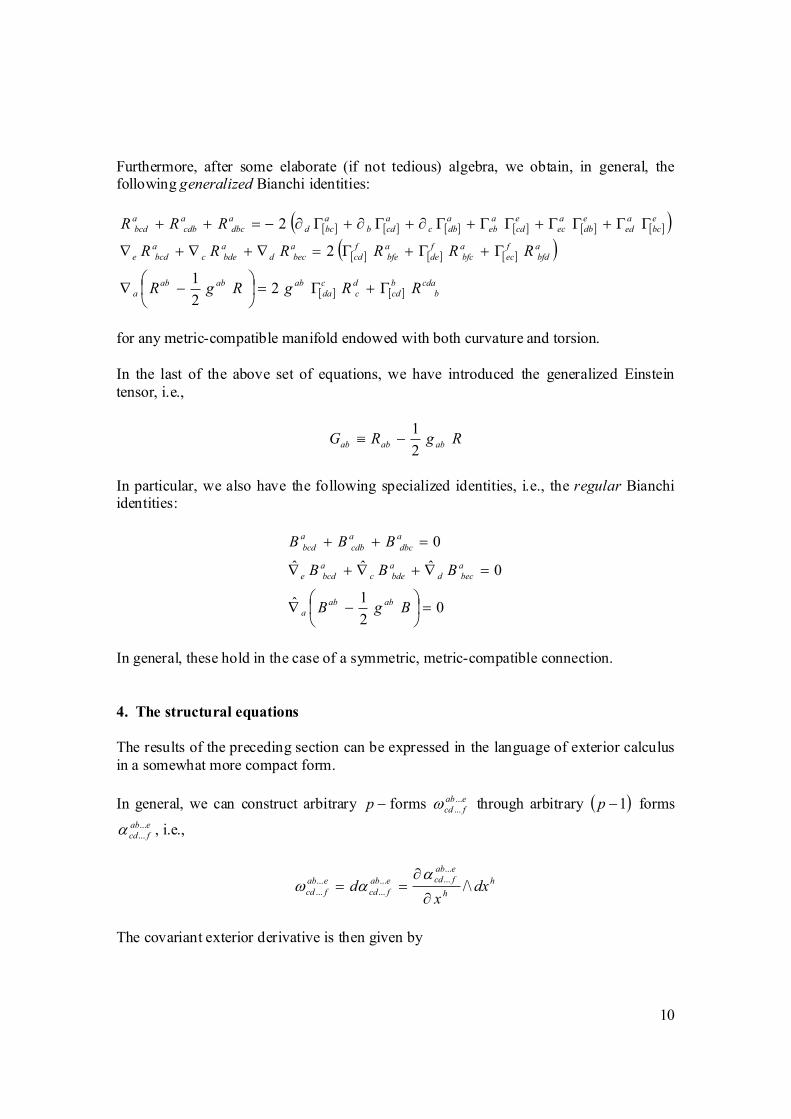
Furthermore, after some elaborate (if not tedious) algebra, we obtain, in general, the following generalized Bianchi identities:
[ ] [ ] [ ] [ ] [ ] [ ]( )[ ] [ ] [ ]( )
[ ] [ ]cda
b
b
cd
d
c
c
da
ababab
a
a
bfd
f
ec
a
bfc
f
de
a
bfe
f
cd
a
becd
a
bdec
a
bcde
e
bc
a
ed
e
db
a
ec
e
cd
a
eb
a
dbc
a
cdb
a
bcd
a
dbc
a
cdb
a
bcd
RRgRgR
RRRRRR
RRR
Γ+Γ=
−∇
Γ+Γ+Γ=∇+∇+∇
ΓΓ+ΓΓ+ΓΓ+Γ∂+Γ∂+Γ∂−=++
22
1
2
2
for any metric-compatible manifold endowed with both curvature and torsion.
In the last of the above set of equations, we have introduced the generalized Einstein
tensor, i.e.,
RgRG ababab2
1−≡
In particular, we also have the following specialized identities, i.e., the regular Bianchi identities:
02
1ˆ
0ˆˆˆ
0
=
−∇
=∇+∇+∇
=++
BgB
BBB
BBB
abab
a
a
becd
a
bdec
a
bcde
a
dbc
a
cdb
a
bcd
In general, these hold in the case of a symmetric, metric-compatible connection.
4. The structural equations
The results of the preceding section can be expressed in the language of exterior calculus
in a somewhat more compact form.
In general, we can construct arbitrary −p forms eab
fcd
...
...ω through arbitrary ( )1−p forms
eab
fcd
...
...α , i.e.,
h
h
eab
fcdeab
fcd
eab
fcd dxx
d /\
...
......
...
...
... ∂
∂==
ααω
The covariant exterior derivative is then given by

11
heab
fcdh
eab
fcd dxD /\...
...
...
... ωω ∇=
i.e.,
( ) ()hfeab
hcd
h
d
eab
fch
h
c
eab
fhd
e
h
hab
fcd
b
h
eah
fcd
a
h
ehb
fcd
peab
fcd
eab
fcd dD
Γ−−Γ−Γ−
Γ++Γ+Γ−+=
/\.../\/\
/\.../\/\1
...
...
...
...
...
...
...
...
...
...
...
...
...
...
...
....
ωωω
ωωωωω
where we have defined the connection one-forms by
ca
bc
a
b θΓ≡Γ
with respect to the coframe basis aθ .
Now we write the torsion two-forms aτ as
ba
b
aaa dD θθθτ /\Γ+==
This gives the first structural equation. With respect to another local coordinate system
(with coordinates αx ) in
∞C spanned by the basis a
ae θε αα = , we see that
[ ]λβα
βλα εετ /\Γ−= aa e
We shall again proceed to define the curvature tensor. For a triad of arbitrary vectors
wvu ,, , we may define the following relations with respect to the frame basis aω :
( )[ ] ( )b
c
cb
c
ca
bvu
a
a
b
b
c
c
vu
uvvuww
wvuw
∇−∇∇≡∇
∇∇≡∇∇
,
ω
where u∇ and v∇ denote covariant differentiation in the direction of u and of v ,
respectively.
Then we have
( ) a
dcba
bcduvvu vuwRw ω*=∇∇−∇∇
Note that
[ ]
[ ]a
be
e
cd
a
bcd
a
be
e
cd
a
ed
e
bc
a
ec
e
bd
a
bcd
a
bdc
a
bcd
R
R
ΓΓ+=
ΓΓ+ΓΓ−ΓΓ+Γ∂−Γ∂=
2
2*
12
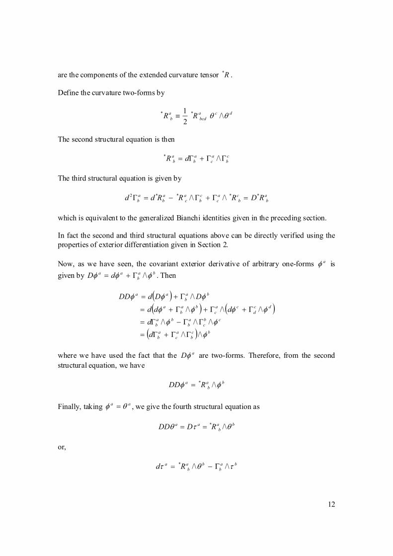
are the components of the extended curvature tensor R* .
Define the curvature two-forms by
dca
bcd
a
b RR θθ /\2
1 ** ≡
The second structural equation is then
c
b
a
c
a
b
a
b dR ΓΓ+Γ= /\*
The third structural equation is given by
a
b
c
b
a
c
c
b
a
c
a
b
a
b RDRRRdd ****2 /\/\ =Γ+Γ−=Γ
which is equivalent to the generalized Bianchi identities given in the preceding section.
In fact the second and third structural equations above can be directly verified using the
properties of exterior differentiation given in Section 2.
Now, as we have seen, the covariant exterior derivative of arbitrary one-forms aφ is
given by ba
b
aa dD φφφ /\Γ+= . Then
( )( ) ( )
( ) bc
b
a
c
a
b
cb
c
a
b
ba
b
dc
d
ca
c
ba
b
a
ba
b
aa
d
d
ddd
DDdDD
φ
φφ
φφφφ
φφφ
/\/\
/\/\/\
/\/\/\
/\
ΓΓ+Γ=
ΓΓ−Γ=
Γ+Γ+Γ+=
Γ+=
where we have used the fact that the aDφ are two-forms. Therefore, from the second
structural equation, we have
ba
b
a RDD φφ /\*=
Finally, taking aa θφ = , we give the fourth structural equation as
ba
b
aa RDDD θτθ /\*==
or,
ba
b
ba
b
a Rd τθτ /\/\* Γ−=

13
Remarkably, this is equivalent to the first generalized Bianchi identity given in the
preceding section.
The elegant results in this section are especially due to E. Cartan. Thanks to his intuitive genius!
5. The geometry of distant parallelism
Let us now consider a special situation in which our −n dimensional manifold ∞C is
embedded isometrically in a flat −n dimensional (pseudo-)Euclidean space nE (with
coordinates mv ) spanned by the constant basis me whose dual is denoted by
ns . This
embedding allows us to globally cover the manifold ∞C in the sense that its geometric
structure can be parametrized by the Euclidean basis me satisfying
( )1,...,1,1, ±±±== diagee nmnmη
It is important to note that this situation is different from the one presented in Section 1,
in which case we may refer the structural equations of ∞C to the locally flat tangent
space )(MTx . The results of the latter situation (i.e., the localized structural equations)
should not always be regarded as globally valid since the tangent space )(MTx , though
ubiquitous in the sense that it can be defined everywhere (at any point) in ∞C , cannot
cover the whole structure of the curved manifold ∞C without changing orientation from
point to point.
One can construct geometries with special connections that will give rise to what we call
geometries with parallelism. Among others, the geometry of distant parallelism is a
famous case. Indeed, A. Einstein adopted this geometry in one of his attempts to geometrize physics, and especially to unify gravity and electromagnetism. In its
application to physical situations, the resulting field equations of a unified field theory based on distant parallelism, for instance, are quite remarkable in that the so-called
energy-momentum tensor appears to be geometrized via the torsion tensor. We will
therefore dedicate this section to a brief presentation of the geometry of distant parallelism in the language of Riemann-Cartan geometry.
In this geometry, it is possible to orient vectors such that their directions remain invariant
after being displaced from a point to some distant point in the manifold. This situation is
made possible by the vanishing of the curvature tensor, which is given by the integrability condition
( ) 0=∂∂−∂∂= m
abccb
d
m
d
abc eeR
where the connection is now given by

14
m
ab
c
m
c
ab ee ∂=Γ
where m
a
m
ae ξ∂= and a
m
a
m xe ∂= .
However, while the curvature tensor vanishes, one still has the torsion tensor given by
[ ] ( )m
cb
m
bc
a
m
a
bc eee ∂−∂=Γ2
1
with the m
ae acting as the components of a spin “potential”. Thus the torsion can now be
considered as the primary geometric object in the manifold ∞pC endowed with distant
parallelism.
Also, in general, the Riemann-Christoffel curvature tensor is non-vanishing as
d
eb
e
ac
d
ec
e
ab
d
acb
d
abc
d
abc KKKKKKB −+∇−∇= ˆˆ
Let us now consider some facts. Taking the covariant derivative of the tetrad m
ae with
respect to the Christoffel symbols alone, we have
c
ab
m
c
d
ab
m
d
m
ab
m
ab Keeee =∆−∂=∇
i.e.,
c
mb
m
a
m
ab
c
m
c
ab eeeeK ∇−=∇= ˆˆ
In the above sense, the components of the contorsion tensor give the so-called Ricci
rotation coefficients. Then from
( )d
ec
e
ab
d
abc
m
d
m
abc KKKee +∇=∇∇ ˆˆˆ
it is elementary to show that
( ) d
abc
m
d
m
acbbc Bee =∇∇−∇∇ ˆˆˆˆ
Likewise, we have
c
mb
m
a
m
ab
c
m
c
ab
c
ab
m
c
d
ab
m
d
m
ab
m
ab
eeee
eKeee
∇−=∇=∆
∆=−∂=∇~~
~

15
where now ∇~ denotes covariant differentiation with respect to the Ricci rotation
coefficients alone. Then from
( )d
ec
e
ab
d
abc
m
d
m
abc ee ∆∆+∆∇=∇∇~~~
we get
( ) [ ]( )d
eb
e
ac
d
ec
e
ab
d
eb
e
ac
d
ec
e
ab
e
bc
d
ae
d
abc
m
d
m
acbbc KKKKBee ∆+∆−∆+∆−Γ∆−−=∇∇−∇∇ 2~~~~
In this situation, one sees, with respect to the coframe basis ma
m
a se=θ , that
aba
b
a Td ≡Γ−= θθ /\
i.e.,
[ ]cba
bc
aT θθ /\Γ=
Thus the torsion two-forms of this geometry are now given by aT (instead of aτ of the
preceding section). We then realize that
0=aDθ
Next, we see that
( )ba
b
bc
b
a
c
a
b
ba
b
ba
b
aa
R
d
dddTd
θ
θ
θθθ
/\
/\/\
/\/\
*
2
−=
ΓΓ+Γ−=
Γ+Γ−==
But, as always, 02 =ad θ , and therefore we have
0/\* =ba
bR θ
Note that in this case, 0* ≠abR as
[ ]a
be
e
cd
a
bcdR ΓΓ= 2*
will not vanish in general. We therefore see immediately that
0*** =++ a
dbc
a
cdb
a
bcd RRR
16
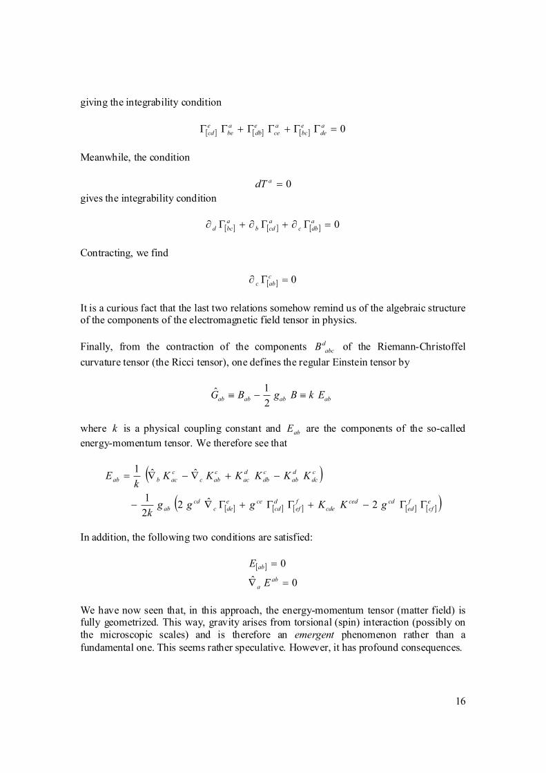
giving the integrability condition
[ ] [ ] [ ] 0=ΓΓ+ΓΓ+ΓΓ a
de
e
bc
a
ce
e
db
a
be
e
cd
Meanwhile, the condition
0=adT
gives the integrability condition
[ ] [ ] [ ] 0=Γ∂+Γ∂+Γ∂ a
dbc
a
cdb
a
bcd
Contracting, we find
[ ] 0=Γ∂ c
abc
It is a curious fact that the last two relations somehow remind us of the algebraic structure of the components of the electromagnetic field tensor in physics.
Finally, from the contraction of the components d
abcB of the Riemann-Christoffel
curvature tensor (the Ricci tensor), one defines the regular Einstein tensor by
abababab EkBgBG ≡−≡2
1ˆ
where k is a physical coupling constant and abE are the components of the so-called
energy-momentum tensor. We therefore see that
( )
[ ] [ ] [ ] [ ] [ ]( )e
cf
f
ed
cdced
cde
f
ef
d
cd
cee
dec
cd
ab
c
dc
d
ab
c
db
d
ac
c
abc
c
acbab
gKKgggk
KKKKKKk
E
ΓΓ−+ΓΓ+Γ∇−
−+∇−∇=
2ˆ22
1
ˆˆ1
In addition, the following two conditions are satisfied:
[ ]
0ˆ
0
=∇
=ab
a
ab
E
E
We have now seen that, in this approach, the energy-momentum tensor (matter field) is fully geometrized. This way, gravity arises from torsional (spin) interaction (possibly on
the microscopic scales) and is therefore an emergent phenomenon rather than a
fundamental one. This seems rather speculative. However, it has profound consequences.
17
6. Spin frames
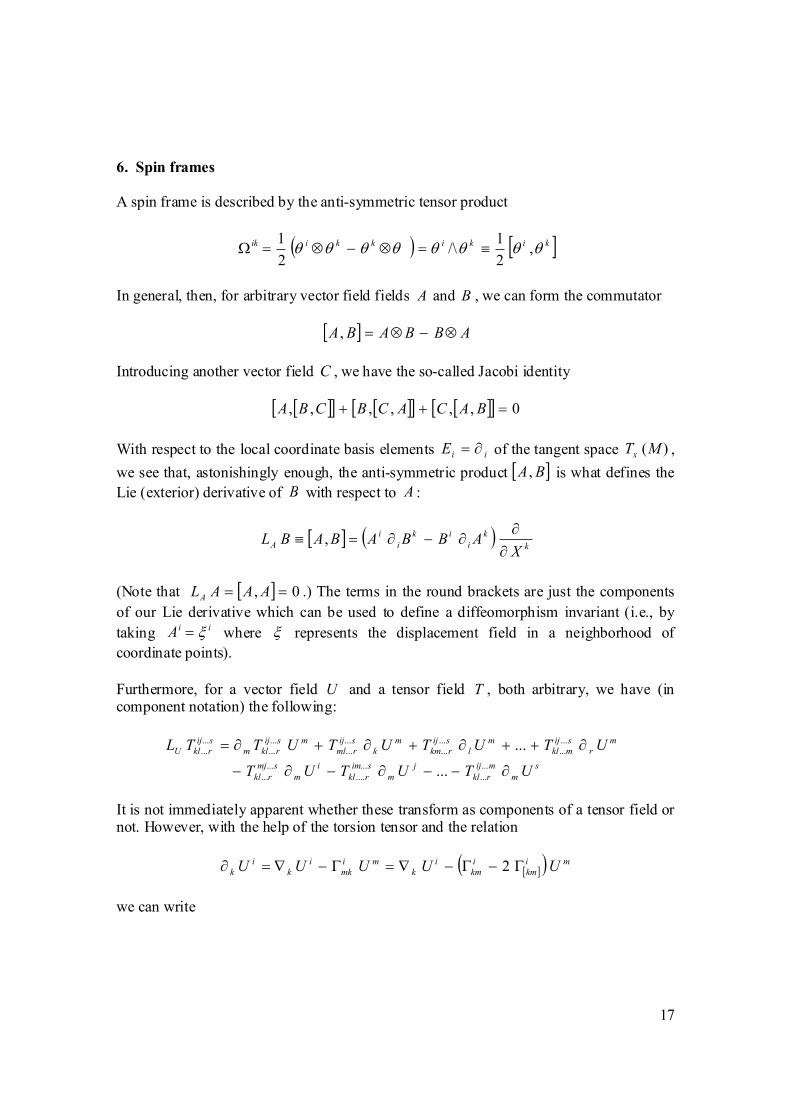
A spin frame is described by the anti-symmetric tensor product
( ) [ ]kikikkiik θθθθθθθθ ,2
1/\
2
1≡=⊗−⊗=Ω
In general, then, for arbitrary vector field fields A and B , we can form the commutator
[ ] ABBABA ⊗−⊗=,
Introducing another vector field C , we have the so-called Jacobi identity
[ ][ ] [ ][ ] [ ][ ] 0,,,,,, =++ BACACBCBA
With respect to the local coordinate basis elements iiE ∂= of the tangent space )(MTx ,
we see that, astonishingly enough, the anti-symmetric product [ ]BA, is what defines the
Lie (exterior) derivative of B with respect to A :
[ ] ( )k
k
i
ik
i
i
AX
ABBABABL∂
∂∂−∂=≡ ,
(Note that [ ] 0, == AAALA .) The terms in the round brackets are just the components
of our Lie derivative which can be used to define a diffeomorphism invariant (i.e., by
taking iiA ξ= where ξ represents the displacement field in a neighborhood of
coordinate points).
Furthermore, for a vector field U and a tensor field T , both arbitrary, we have (in component notation) the following:
s
m
mij
rkl
j
m
sim
rkl
i
m
smj
rkl
m
r
sij
mkl
m
l
sij
rkm
m
k
sij
rml
msij
rklm
sij
rklU
UTUTUT
UTUTUTUTTL
∂−−∂−∂−
∂++∂+∂+∂=...
...
...
....
...
...
...
...
...
...
...
...
...
...
...
...
...
...
It is not immediately apparent whether these transform as components of a tensor field or not. However, with the help of the torsion tensor and the relation
[ ]( ) mi
km
i
km
i
k
mi
mk
i
k
i
k UUUUU Γ−Γ−∇=Γ−∇=∂ 2
we can write
18
[ ] [ ] [ ]
[ ] [ ] [ ]psij
mkl
m
rp
psij
rkm
m
lp
psij
rml
m
kp
pmij
rkl
s
mp
psim
rkl
j
mp
psmj
rkl
i
mp
s
m
mij
rkl
j
m
sim
rkl
i
m
smj
rkl
m
r
sij
mkl
m
l
sij
rkm
m
k
sij
rml
msij
rklm
sij
rklU
UTUTUT
UTUTUT
UTUTUT
UTUTUTUTTL
...
...
...
...
..
...
...
...
...
...
...
...
...
...
...
....
...
...
...
...
...
...
...
...
...
...
...
...
2...22
2...22
...
...
Γ−−Γ−Γ−
Γ++Γ+Γ+
∇−−∇−∇−
∇++∇+∇+∇=
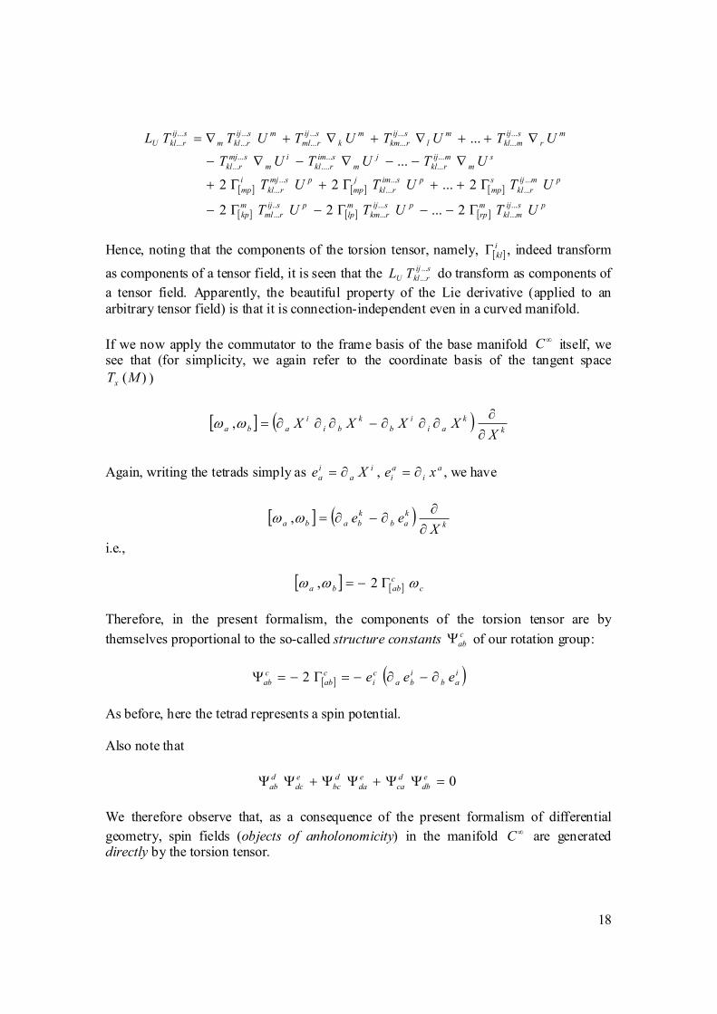
Hence, noting that the components of the torsion tensor, namely, [ ]i
klΓ , indeed transform
as components of a tensor field, it is seen that the sij
rklU TL...
... do transform as components of
a tensor field. Apparently, the beautiful property of the Lie derivative (applied to an
arbitrary tensor field) is that it is connection-independent even in a curved manifold.
If we now apply the commutator to the frame basis of the base manifold ∞C itself, we
see that (for simplicity, we again refer to the coordinate basis of the tangent space
)(MTx )
[ ] ( )k
k
ai
i
b
k
bi
i
abaX
XXXX∂
∂∂∂∂−∂∂∂=ωω ,
Again, writing the tetrads simply as a
i
a
i
i
a
i
a xeXe ∂=∂= , , we have
[ ] ( )k
k
ab
k
babaX
ee∂
∂∂−∂=ωω ,
i.e.,
[ ] [ ] c
c
abba ωωω Γ−= 2,
Therefore, in the present formalism, the components of the torsion tensor are by
themselves proportional to the so-called structure constants c
abΨ of our rotation group:
[ ] ( )iab
i
ba
c
i
c
ab
c
ab eee ∂−∂−=Γ−=Ψ 2
As before, here the tetrad represents a spin potential.
Also note that
0=ΨΨ+ΨΨ+ΨΨ e
db
d
ca
e
da
d
bc
e
dc
d
ab
We therefore observe that, as a consequence of the present formalism of differential
geometry, spin fields (objects of anholonomicity) in the manifold ∞C are generated directly by the torsion tensor.
19
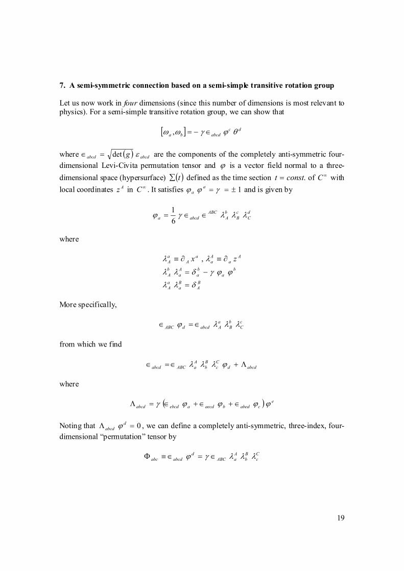
7. A semi-symmetric connection based on a semi-simple transitive rotation group
Let us now work in four dimensions (since this number of dimensions is most relevant to physics). For a semi-simple transitive rotation group, we can show that
[ ] dc
abcdba θϕγωω ∈−=,
where ( ) abcdabcd g εdet=∈ are the components of the completely anti-symmetric four-
dimensional Levi-Civita permutation tensor and ϕ is a vector field normal to a three-
dimensional space (hypersurface) ( )t∑ defined as the time section .constt = of ∞C with
local coordinates Az in ∞C . It satisfies 1±== γϕϕ a
a and is given by
d
C
c
B
b
A
ABC
abcda λλλγϕ ∈∈=6
1
where
B
A
B
a
a
A
b
a
b
a
A
a
b
A
A
a
A
a
a
A
a
A zx
δλλ
ϕϕγδλλ
λλ
=
−=
∂≡∂≡ ,
More specifically,
c
C
b
B
a
AabcddABC λλλϕ ∈=∈
from which we find
abcdd
C
c
B
b
A
aABCabcd Λ+∈=∈ ϕλλλ
where
( ) e
cabedbaecdaebcdabcd ϕϕϕϕγ ∈+∈+∈=Λ
Noting that 0=Λ d
abcd ϕ , we can define a completely anti-symmetric, three-index, four-
dimensional “permutation” tensor by
C
c
B
b
A
aABC
d
abcdabc λλλγϕ ∈=∈≡Φ
20
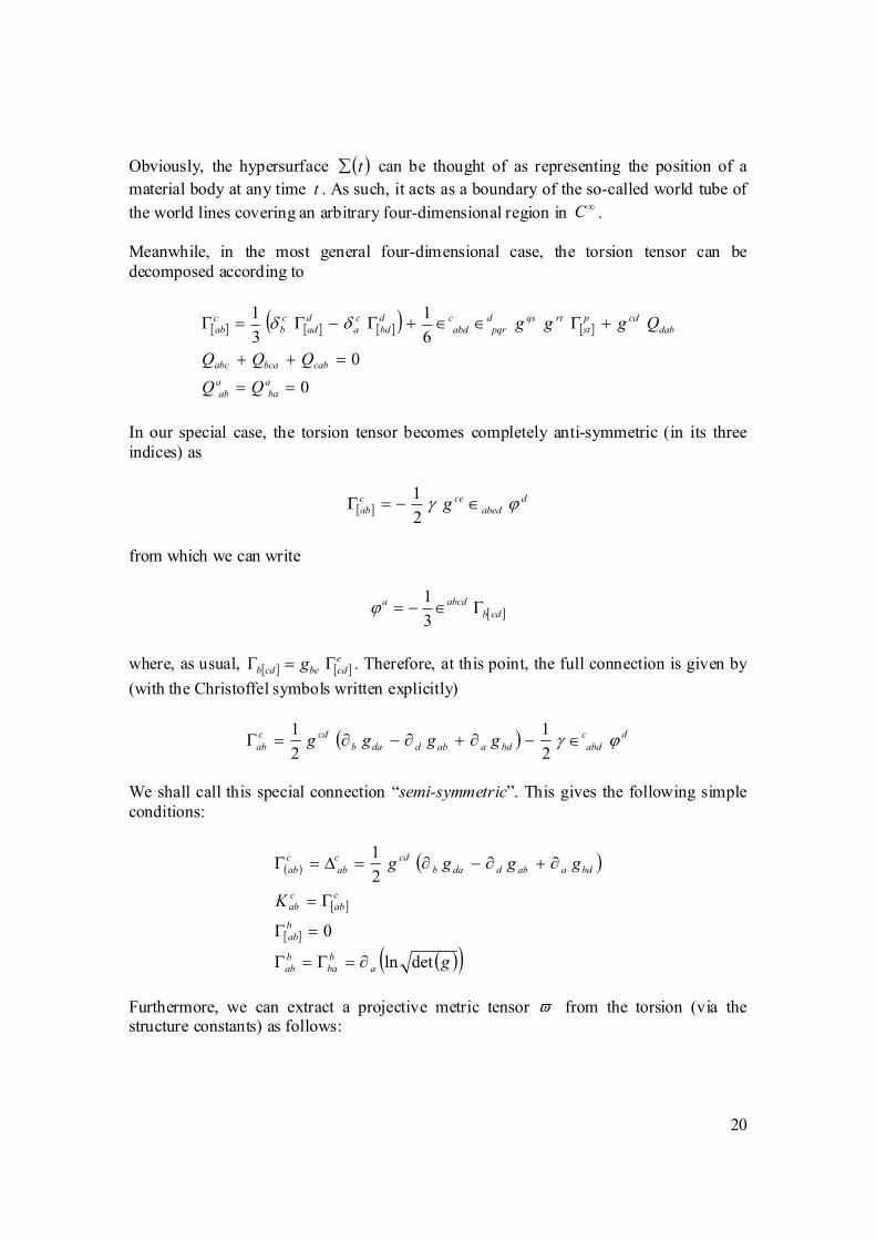
Obviously, the hypersurface ( )t∑ can be thought of as representing the position of a
material body at any time t . As such, it acts as a boundary of the so-called world tube of
the world lines covering an arbitrary four-dimensional region in ∞C .
Meanwhile, in the most general four-dimensional case, the torsion tensor can be
decomposed according to
[ ] [ ] [ ]( ) [ ]
0
0
6
1
3
1
==
=++
+Γ∈∈+Γ−Γ=Γ
a
ba
a
ab
cabbcaabc
dab
cdp
st
rtqsd
pqr
c
abd
d
bd
c
a
d
ad
c
b
c
ab
QQQ
Qgggδδ
In our special case, the torsion tensor becomes completely anti-symmetric (in its three
indices) as
[ ]d
abed
cec
ab g ϕγ ∈−=Γ2
1
from which we can write
[ ]cdb
abcda Γ∈−=3
1ϕ
where, as usual, [ ] [ ]e
cdbecdb g Γ=Γ . Therefore, at this point, the full connection is given by
(with the Christoffel symbols written explicitly)
( ) dc
abdbdaabddab
cdc
ab gggg ϕγ ∈−∂+∂−∂=Γ2
1
2
1
We shall call this special connection “semi-symmetric”. This gives the following simple
conditions:
( ) ( )
[ ]
[ ]
( )( )g
K
gggg
a
b
ba
b
ab
b
ab
c
ab
c
ab
bdaabddab
cdc
ab
c
ab
detln
0
2
1
∂=Γ=Γ
=Γ
Γ=
∂+∂−∂=∆=Γ
Furthermore, we can extract a projective metric tensor ϖ from the torsion (via the structure constants) as follows:
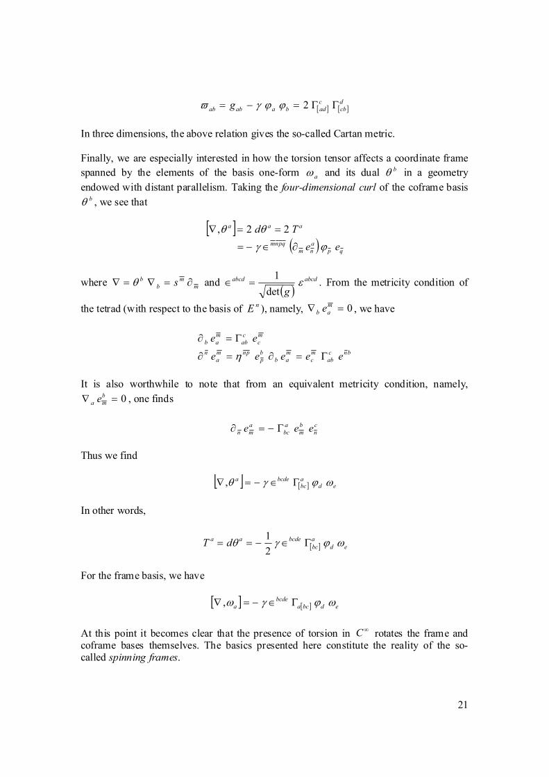
21
[ ] [ ]d
cb
c
adbaabab g ΓΓ=−= 2ϕϕγϖ
In three dimensions, the above relation gives the so-called Cartan metric.
Finally, we are especially interested in how the torsion tensor affects a coordinate frame
spanned by the elements of the basis one-form aω and its dual bθ in a geometry
endowed with distant parallelism. Taking the four-dimensional curl of the coframe basis bθ , we see that
[ ]( ) qp
a
nm
qpnm
aaa
ee
Td
ϕγ
θθ
∂∈−=
==∇ 22,
where m
m
b
b s ∂=∇=∇ θ and ( )
abcdabcd
gε
det
1=∈ . From the metricity condition of
the tetrad (with respect to the basis of n
E ), namely, 0=∇ m
ab e , we have
bnc
ab
m
c
m
ab
b
p
pnm
a
n
m
c
c
ab
m
ab
eeeee
ee
Γ=∂=∂
Γ=∂
η
It is also worthwhile to note that from an equivalent metricity condition, namely,
0=∇ b
ma e , one finds
c
n
b
m
a
bc
a
mn eee Γ−=∂
Thus we find
[ ] [ ] edabc
bcdea ωϕγθ Γ∈−=∇ ,
In other words,
[ ] ed
a
bc
bcdeaadT ωϕγθ Γ∈−==
2
1
For the frame basis, we have
[ ] [ ] edbca
bcde
a ωϕγω Γ∈−=∇ ,
At this point it becomes clear that the presence of torsion in ∞C rotates the frame and
coframe bases themselves. The basics presented here constitute the reality of the so-called spinning frames.
22
Suggested general references In writing this article, I have had to rely on my own intuition (mental construct), understanding, and memory alone without any particular attachment to just one or two of
the well-known works. As for references or further reading, there’s a number of widely
appreciated books and articles on differential geometry. I myself have come across some of them. Their in-depth presentation of the subject provides excellent educational
material. Also, I feel that it is important to get a sense of history and so reading the
writings of the founding fathers of (modern) differential geometry (especially Cartan’s
writings) is essential. One may compare the present work to the following general
references (most of them, especially the later ones, are more advanced):
C. F. Gauss, Collected Works, Princeton (translation), 1902.
T. Levi-Civita, The Absolute Differential Calculus, Blackie, Glasgow and London, 1927.
O. Veblen, Invariants of Quadratic Differential Forms, Cambridge Univ. Press, London
and New York, 1927. E. Cartan, Les systémes différentials extérieurs et leurs applications géométriques,
Actualités scientifiques 994, Paris, 1945. B. Riemann, Collected Works, Dover, New York, 1953.
H. Rund, The Differential Geometry of Finsler Spaces, Springer, Berlin-Copenhagen-
Heidelberg, 1959.
H. Cartan, Formes différentielles, Hermann, Paris, 1967.
W. Greub, S. Halperin, and R. Vanstone, Connections, Curvature and Cohomology, Vol. I, Academic Press, New York, 1972.