Embed Size (px)
Citation preview
A Computational Method for Determining Distributed Aerodynamic Loads on Planforms
of Arbitrary Shape in Compressible Subsonic Flow
By:
Matthew Alan Brown
B.S. Aerospace Engineering, University of Kansas, 2009
Submitted to the Graduate Degree Program in Aerospace Engineering and the Graduate Faculty of the University of Kansas in Partial Fulfillment of the Requirements for the
Degree of Master of Science in Aerospace Engineering.
______________________________________
Chairperson: Dr. Ray Taghavi
_____________________________________
Dr. Saeed Farokhi
____________________________________
Dr. Shawn Keshmiri
Date Defended: 12/11/2013
ii
The Thesis Committee for Matthew Alan Brown
Certifies that this is the Approved Version of the Following Thesis:
___________________________________
Chairperson: Dr. Ray Taghavi
Date approved: 12/11/2013
A Computational Method for Determining Distributed Aerodynamic Loads on Planforms
of Arbitrary Shape in Compressible Subsonic Flow
iii
Abstract
The methods presented in this work are intended to provided an easy to understand and easy to
apply method for determining the distributed aerodynamic loads and aerodynamic characteristics
of planforms of nearly arbitrary shape. Through application of the cranked wing approach, most
planforms can be modeled including nearly all practical lifting surfaces with some notable
exceptions. The methods are extremely accurate for elliptic wings and rectangular wings with
some notable difficulty attributed to swept wings and wings with control surface deflection. A
method for accounting for the shift in the locus of aerodynamic centers is also presented and
applied to the lifting line theory to mitigate singularities inherent in its formulation.
Comparisons to other numerical methods as well as theoretical equations and experimental data
suggest that the method is reasonably accurate, but limited by some of its contributing theories.
Its biggest benefit is its ability to estimate viscous effects which normally require more
sophisticated models.

iv
Acknowledgements
First and foremost I would like to thank my loving soon-to-be wife Chelsea Magruder for her
undying support while I worked my way through graduate school and my mother for untold
financial, emotional, and academic advice. Without their seemingly infinite patience I am not
sure any of this would have been possible. I would also like to thank Dr. Ray Taghavi for his
advice and guidance not just on this project, but on countless topics throughout my academic
career. Also, Dr. Saeed Farokhi and Dr. Shawn Keshmiri for their advice and support. Lastly, I
would like to thank my friends and family who have put up with me for this long. I know how
difficult that can be and I do appreciate it.

v
Table of Contents
Abstract ......................................................................................................................................... iii
Acknowledgements ...................................................................................................................... iv
Table of Contents .......................................................................................................................... v
List of Figures .............................................................................................................................. vii
List of Symbols ............................................................................................................................. ix
List of Symbols Cont… ................................................................................................................. x
List of Symbols Cont… ................................................................................................................ xi
List of Symbols Cont… ............................................................................................................... xii
List of Symbols Cont… .............................................................................................................. xiii
List of Subscripts........................................................................................................................ xiii
List of Acronyms ........................................................................................................................ xiv
1. Introduction ........................................................................................................................... 1
1.1 Objectives ......................................................................................................................... 1
1.2 Background ...................................................................................................................... 1
1.3 Motivation ........................................................................................................................ 2
2. Review of Current Literature and Methods ....................................................................... 3
2.1 Airfoil Analysis ................................................................................................................ 3
2.2 Lifting Line Theory .......................................................................................................... 6
2.3 Vortex Lattice Method ..................................................................................................... 9
2.4 3D Panel Methods .......................................................................................................... 11
2.5 Navier-Stokes Equations ................................................................................................ 12
2.6 MIAReX and XFLR5 ..................................................................................................... 14
2.7 Wind Tunnel Testing ...................................................................................................... 15
2.8 Conclusions .................................................................................................................... 16
3. Theoretical Development .................................................................................................... 17
3.1 Overview ........................................................................................................................ 17
3.2 Chord Loading ................................................................................................................ 18
3.3 Span Loading .................................................................................................................. 28
3.4 Aerodynamic Center ...................................................................................................... 35
3.5 Forces, Moments and Coefficients ................................................................................. 40
4. Application ........................................................................................................................... 43
4.1 Computational Considerations ....................................................................................... 43
vi
4.2 Post Processing and Visualization.................................................................................. 46
4.3 Advanced Planform Analysis and XFOILultra .............................................................. 52
5. Discussion of Results ........................................................................................................... 53
5.1 Experimental Validation: Extended Tangent Approximation ........................................ 53
5.2 Theoretical Validation : Elliptic Wing ........................................................................... 54
5.3 Theoretical and Experimental Validation: Rectangular Wings ..................................... 57
5.4 Theoretical and Experimental Validation: Swept Wings ............................................... 62
5.5 Experimental Validation: Wing with Control Surface Deflection ................................. 69
5.6 Design Application: The Winglet Problem .................................................................... 74
6. Conclusions and Recommendations .................................................................................. 79
6.1 Conclusions .................................................................................................................... 79
6.2 Recommendations .......................................................................................................... 80
7. References............................................................................................................................. 82
Appendix A-MATLAB Code ..................................................................................................... 86
vii
List of Figures
Figure 2.1 Basic Thin Airfoil Theory7 ......................................................................................................... 3
Figure 2.2 Calculation Scheme of XFOIL14 ................................................................................................ 6
Figure 2.3 Lanchester/Prandtl Hypothesis7 .................................................................................................. 7
Figure 2.4 Visual Description of Elliptic Wing Problem7 ........................................................................... 8
Figure 2.5 Layout of Vortex Lattice System .............................................................................................. 10
Figure 2.6 Panel Model of MD-11 at Take-Off37....................................................................................... 12
Figure 2.7 Example of High Fidelity CFD Results40 ................................................................................. 14
Figure 2.8 Example of High Quality Wind Tunnel Model45 ...................................................................... 16
Figure 3.1 Comparison of XFOIL to Experimental Data for a NACA 4415 Airfoil ................................. 23
Figure 3.2 Airfoil Data Extrapolated via Viterna Method, NACA 4415 at Re=3e6 and AR=10 .............. 25
Figure 3.3 Contribution of Pressure and Friction to Axial Force for NACA 4415 at Re=3e6 .................. 26
Figure 3.4 Extreme Angle of Attack Flat Plate Pressure and Friction Distribution Assumptions ............. 27
Figure 3.5 Predicted Pressure and Skin Friction Distribution on NACA4415 at Re=3e6 ......................... 27
Figure 3.6 Example Wing Vortex System ................................................................................................. 28
Figure 3.7 Velocity Induced by Horseshoe Vortex .................................................................................... 29
Figure 3.8 Definition of Discritized Geometric Properties ........................................................................ 31
Figure 3.9 Dihedral and Incidence Angle Definitions ............................................................................... 32
Figure 3.10 Küchemann A.C. Shift Parameters ......................................................................................... 37
Figure 3.11 Extended Küchemann A.C. Shift Parameters ......................................................................... 38
Figure 3.12 Extended Prandtl Hypothesis .................................................................................................. 41
Figure 4.1 Cranked Panel Definitions ........................................................................................................ 45
Figure 4.2 Quad-Mesh Parameters ............................................................................................................. 50
Figure 4.3 Example of Meshing Procedure Results ................................................................................... 50
Figure 5.1 Comparison of Tangent Approximations to Experimental Data .............................................. 54
Figure 5.2 Predicted and Theoretical Circulation on Elliptic Wings, α=5˚, Re=2.4e6 .............................. 56
Figure 5.3 Predicted and Theoretical Induced Drag Polar for Elliptic Wings, Re=2.4e6 .......................... 57
Figure 5.4 Predicted and Theoretical Lift Curve Slope for Elliptic Wings, Re=2.4e6 .............................. 57
Figure 5.5 Predicted and Theoretical Lift Curve Slope for Rectangular Wings, Re=2.4e6 ....................... 58
Figure 5.6 Calculated Induced Drag Polars for Rectangular Wings, Re=2.4e6 ......................................... 59
Figure 5.7 Predicted and Experimental Load Distribution on Square Wing, α=4˚ .................................... 59
Figure 5.8 Predicted and Experimental Load Distribution on Square Wing, α=8˚ .................................... 60
Figure 5.9 Predicted andExperimental Load Distribution on Square Wing, α=12˚ ................................... 60

viii
Figure 5.10 Predicted and Experimental Pressure Distribution on Square Wing, α=4˚............................. 61
Figure 5.11 Predicted and Experimental Lift Curve Slopes for Swept Wings, AR=5.13, Re=2.5e5 ........ 62
Figure 5.12 Predicted and Experimental Drag Polars for Untapered Wing, AR=5.13, Λ=0˚, Re=2.5e5 .. 63
Figure 5.13 Predicted and Experimental Drag Polars for Untapered Wing, AR=5.13, Λ=15˚, Re=2.5e5 64
Figure 5.14 Predicted and Experimental Drag Polars for Untapered Wing, AR=5.13, Λ=30˚, Re=2.5e5 64
Figure 5.15 Predicted and Experimental Drag Polars for Untapered Wing, AR=5.13, Λ=45˚, Re=2.5e5 65
Figure 5.16 Predicted and Experimental Normal Force Distribution on Swept Wings, AR=5.13, α=8.5˚ 66
Figure 5.17 Predicted Pressure Distribution on Untapered Wing, Λ=0˚, AR=5.13, α=8.5˚, Re=2.5e5 ..... 67
Figure 5.18 Predicted Pressure Distribution on Untapered Wing, Λ=15˚, AR=5.13, α=8.5˚, Re=2.5e5 ... 67
Figure 5.19 Predicted Pressure Distribution on Untapered Wing, Λ=30˚, AR=5.13, α=8.5˚, Re=2.5e5 ... 68
Figure 5.20 Predicted Pressure Distribution on Untapered Wing, Λ=45˚, AR=5.13, α=8.5˚, Re=2.5e5 ... 68
Figure 5.21 Lift and Drag Data for Rectangular Wing with Half-Span Flaps, δf=0˚, AR=3.13 ............... 70
Figure 5.22 Lift and Drag Data for Rectangular Wing with Half-Span Flaps, δf=10˚, AR=3.13 ............. 70
Figure 5.23 Lift and Drag Data for Rectangular Wing with Half-Span Flaps, δf=20˚, AR=3.13 ............. 71
Figure 5.24 Predicted Pressure Distribution on Rectangular Wing with Half-Span Flaps, δf=0˚ ............. 72
Figure 5.25 Predicted Pressure Distribution on Rectangular Wing with Half-Span Flaps, δf=10˚ ........... 73
Figure 5.26 Predicted Pressure Distribution on Rectangular Wing with Half-Span Flaps, δf=20˚ ........... 73
Figure 5.27 APA Predicted Lift and Drag Characteristics of Modified Wing, Sref=91.675 ft2 .................. 75
Figure 5.28 VLM Predicted Lift and Drag Characteristics of Modified Wing, Sref=91.675 ft2 ................. 75
Figure 5.29 XFLR5 Predicted Lift and Drag Characteristics of Modified Wing, Sref=91.675 ft2 .............. 76
Figure 5.30 APA Predicted Pressure and Skin Friction, Unmodified Wing, α=5˚, Re=2.9e6 ................... 77
Figure 5.31 APA Predicted Pressure and Skin Friction, Wing with Winglet, α=5˚, Re=2.9e6 ................. 77
Figure 5.32 XFLR5 Predicted Pressure and Skin Friction, α=5˚, Re=2.9e6 .............................................. 78
ix
List of Symbols
Symbol Description Units
0A Coefficient of Class-I Drag Polar ~
1A Coefficient of Class-I Drag Polar ~
2A Coefficient for Viterna Method ~
AR Aspect Ratio ~
SA Area of Surface Element ft2
2B Coefficient for Viterna Method ~
1CDB Coefficient of Class-II Drag Polar ~
2CDB Coefficient of Class-II Drag Polar ~
3CDB Coefficient of Class-II Drag Polar ~
4CDB Coefficient of Class-II Drag Polar ~
5CDB Coefficient of Class-II Drag Polar ~
DC Planform Drag Coefficient ~ *
DC Dissipation Coefficient ~
iDC Planform Induced Drag Coefficient ~
LC Planform Lift Coefficient ~
lC Planform Rolling Moment Coefficient ~
LC
Planform Lift Curve Slope rad-1
0LC Planform Lift Coefficient at Zero Angle of Attack ~
mC Planform Pitching Moment Coefficient ~
0mC Planform Pitching Moment Coefficient at Zero Angle of Attack ~
0mC Planform Pitching Moment Coefficient at Zero Lift Angle of Attack ~
mC
Planform Pitching Moment Curve Slope rad-1
YC Planform Side Force Coefficient ~
C Maximum Shear Stress Coefficient ~
'D Section Lift Force lb/ft
F
Global Force Vector lb
G Non-dimensional Vortex Strength ~
H Boundary Layer Shape Parameter ~ *H Boundary Layer Shape Parameter ~ **H Boundary Layer Shape Parameter ~

x
List of Symbols Cont…
Symbol Description Units
kH Boundary Layer Shape Parameter ~
J Newton Corrector Matrix ~
'L Section Drag Force lb
M
Global Moment Vector ft-lb
afM Number of Spanwise Stations for Surface Plots ~
afN Number of Chordwise Stations for Surface Plots ~
panN Number of Control Points & Elements in Cranked Wing Panel ~
xP Shape Parameter for Tangent Approximation ~
zP Shape Parameter for Tangent Approximation ~
R Residual Vector ~
Re Reynolds Number ~ Re Reynolds Number based on Momentum Thickness of Boundary Layer ~
S Planform Area ft2
U
Freestream Velocity Vector ft/s
sU Boundary Layer Shape Parameter ~
V
Velocity Vector ft/s
a
Spatial Vector for Surface Mesh ft
b
Spatial Vector for Surface Mesh ft
b Wing Span ft
c
Spatial Vector for Surface Mesh ft
c Chord ft
c Characteristic Chord ft
ac Airfoil Axial Force Coefficient ~
dc Airfoil Drag Coefficient ~
maxdc Maximum Airfoil Drag Coefficient for Viterna Method ~
stalldc Last Available Airfoil Drag Coefficient for Viterna Method ~
fc Skin Friction Coefficient ~
lc Airfoil Lift Coefficient ~
lc
Airfoil Lift Curve Slope rad-1
mc Airfoil Pitching Moment Coefficient ~

xi
List of Symbols Cont…
Symbol Description Units
nc Airfoil Normal Force Coefficient ~
pc Compressible Pressure Coefficient ~
ipc Incompressible Pressure Coefficient ~
d
Spatial Vector for Surface Mesh ft
d Vector for Bound Portion of Vortex ft
e Planform Efficiency Factor ~
f
Local Force Vector lb *ii Local Incidence Angle deg
n Transition Critera ~
n Normal Vector ~ q Freestream Dynamic Pressure psf
1r Vector from Node 1i to Control Point j ft
2r Vector from Node 2i to Control Point j ft
cgr Vector from Control Point j to Center of Gravity ft
s Span Coordinate ft
t Tangent Vector ~
aiu
Local Airfoil Axial Vector ~
diu
Local Airfoil Drag Vector ~
eu Compressible Velocity External to the Boundary Layer ft/s
eiu Incompressible Velocity External to the Boundary Layer ft/s
u X-Component of Freestream Velocity Vector ft/s
u
Non-Dimensional Freestream Velocity Vector ~
liu
Local Airfoil Lift Vector ~
niu
Local Airfoil Normal Vector ~
v Non-Dimensional Induced Velocity Vector ~
1v Sub-Variable of Non-Dimensional Induced Velocity Vector ~
2v Sub-Variable of Non-Dimensional Induced Velocity Vector ~
12v Sub-Variable of Non-Dimensional Induced Velocity Vector ~
xii
aiv Local Velocity in Axial Direction ft/s
v Y-Component of Freestream Velocity Vector ft/s
List of Symbols Cont…
Symbol Description Units
niv Local Velocity in Normal Direction ft/s
iw
Local Induced Velocity Vector ft/s
x X-Coordinate ft/s
x Stability Coordinate ft/s
y Y-Coordinate ft/s
z Z-Coordinate ft/s
Circulation Strength ft2/s
G Change in Predicted Circulation During Iteration ft2/s
acx Shift of Aerodynamic Center in X-Direction ft
acz Shift of Aerodynamic Center in Z-Direction ft
xy Change of Angle in XY-Plane rad
yz Change of Angle in YZ-Plane rad
Sweep Angle rad
Linearized Influence Matrix rad
Stream Function ft2/s
Relaxation Factor ~
Angle of Attack deg
eff Effective Angle of Attack deg
ind Induced Angle of Attack deg
min Reflection Point for Viterna Method deg
0w Planform Zero-Lift Angle of Attack deg
stall Last Available Angle of Attack for Viterna Method deg
c Compressibility Coefficient ~
Surface Bound Vortex Strength (Airfoil Anlaysis) ft2/s
Boundary Layer Thickness ft * Boundary Layer Displacement Thickness ft
A Differential Discretized Planform Area ft2
i Control Surface Deflection Angle deg

xiii
Boundary Layer Coordinate ft
Non-Dimensional Term for Lifting Line Theory ~
List of Symbols Cont…
Symbol Description Units
s Interpolation Factor ~
Boundary Momentum Thickness ft
Hyperbolic Blending Function ~
Freestream Atmospheric Density slug/ft3
Source Strength ft/s
Local Dihedral Angle deg
Local Fluid Vorticity ft2/s
Upper/Lower Surface ~
List of Subscripts
Subscript Description
1 Node Point 1, LHS
2 Node Point 2, RHS
ac Aerodynamic Center
/ 2c Half-Chord
/ 4c Quarter-Chord
,D d Due to Drag
f Due to Friction
,L l Due to Lift
p Due to Pressure
r At Root
t At Tip
x In X-Direction
z In Z-Direction

xiv
List of Acronyms
Acronym Description
3DP 3D Panel Method
APA Advanced Planform Analysis
BEM Blade Element Momentum Analysis
CFD Computational Fluid Dynamics
NACA National Advisory Committee on Aeronautics
VLM Vortex Lattice Method
QVLM Quasi-Vortex Lattice Method
1
1. Introduction
This section summarizes the objectives, background and motivation for the methods presented
herein.
1.1 Objectives
The ultimate objective of this research is to improve the preliminary design process by providing
a simple and easy to understand method for analyzing the aerodynamic characteristics of
planforms of arbitrary shape. By improving the accuracy of these models used early in the
design process it is possible to reduce the amount of redesign and testing usually required later in
design process, especially for configurations with atypical lifting surfaces.
1.2 Background
The origin of this method can be traced back to 2011 where it was conceived as a way to
assemble load sets for Finite Element Analysis (FEA) without the costs associated with
Computational Fluid Dynamics (CFD) analysis and while still providing impressive 3D images
that convey a sense of authority to customers and colleagues. Presented at the 50th AIAA
Aerospace Sciences Meeting, the original formulation1 was limited to straight taper wings with
linear twist and neglected such important factors as induced angle of attack, frictional forces,
control surfaces, and non-linear behavior. Far from a comprehensive approach, it provided a
reasonably accurate method to assemble loads for engineering projects and was eventually
adapted for use with Blade Element Momentum (BEM)2 theory to provide similar load sets for
wind turbine projects.

2
1.3 Motivation
Given the limitations of the original formulation it was clear that a more comprehensive
approach was needed. Research into ways of extending this method began in the winter of 2012
and quickly revealed that techniques for determining spanwise load distribution while varied are
limited to somewhat specific cases. As a result, many of the classical design methods and
equations commonly used for estimating forces and moments on lifting surfaces3,4,5 are subject to
these same limitations as they are based around data gained through application of these
methods. While adequate for most purposes they do not typically satisfy such cases as winglets,
non-linear/non-elliptic chord distributions, or non-planar chord lines.
Solutions for the spanwise distributions of these more difficult cases rely on adaptations of
simpler theories which can be mathematically complex and often overlook important factors
such as aerodynamic center shift, three dimensional flow, viscosity or compressibility. There are
certainly tools capable of some or all of these types of analyses, including Vortex Lattice Method
(VLM), 3-D Panel Methods (3DP) or CFD. However, these can often be difficult to use. It is
hoped that the methods explained in this work and the accompanying MATLAB6 code provide a
way to easily incorporate advanced planform analysis techniques into the preliminary design
process in a meaningful way. The advanced visualization methods and capability to produce
fully distributed 3D loads for FEA only add to the applicability of this method.

3
2. Review of Current Literature and Methods
This section offers a review of relevant literature and methods for the estimation of distributed
aerodynamic loads. Methods for estimating span loading, chord loading and fully distributed
loads are discussed and major advantages and disadvantages of each are identified.
2.1 AirfoilAnalysis
There are several methods for mathematically resolving chordwise loading of airfoils; however,
they can be divided into three main camps. The first is classical thin airfoil theory and can be
found in countless aerodynamics textbooks7,8,9. It relies on placing a bound vortex filament of
unknown and varying strength along the camber line of a given airfoil as shown in Figure 2.1.
By assuming the corresponding stream function follows the camber line and solving for the
strength distribution which satisfies the Kutta condition, the net potential lift on the airfoil can be
calculated. This has the advantage of being very easy to solve and in most cases can be solved
by hand. However, traditional formulations neglect the effects of viscosity which can influence
drag and to a lesser extent the net lift and pitching moment.
Figure 2.1 Basic Thin Airfoil Theory7
4
A modernized version of thin airfoil theory accounting for the effects of viscosity was proposed
by Yates10; however, this method is computationally complex and fails to address the
fundamental flaw of all thin airfoil theories, which is namely airfoil thickness. Airfoil thickness
can influence everything from maximum lift and lift curve slope to boundary layer transition and
flow separation. These effects are often not negligible and should at least be considered when
analyzing any airfoil.
To account for the effects of thickness an approach similar to thin airfoil theory is often used.
However, instead of a vortex filament bound along the camber line, discrete segments are used
which approximate the shape of the airfoil. Along each segment (or panel) is a linear bound
vortex filament of unknown strength, sometimes assumed to be constant and in other cases
allowed to vary linearly or even quadradically. This leads to the term ‘panel method’ and
constitutes the second and most common type of airfoil analysis. Solutions to the panel method
problem are found by assuming that the stream function is actually the superposition of the
stream functions of the freestream cross-flow and each of the bound vortex segments on the
airfoil surface. This method quickly surrenders through a simple matrix inversion and results in
the panel strengths which are easily converted to local velocity and pressure.
A fundamentally different approach known as conformal mapping relies on the Kutta-Joukowski
theorem9. This allows for the known potential function of a rotating circular cylinder in a cross-
flow or other lifting body to be transformed to a given airfoil shape through use of complex
variables. While both approaches yield remarkably similar results, neither formulation accounts
for the effects of viscosity. In order to do this it is necessary to couple the potential flow
calculations obtained using conformal mapping or panel methods with some sort of boundary
5
layer theory. This most commonly takes the form of the Von Kármán Momentum Integral
equation9 which relates several characteristics of the boundary layer flow to the nearly potential
flow outside of the boundary layer.
Several well known and widely used methods for airfoil design and analysis make use of this
coupled approach. The simplest of these methods used by Eppler11 and Hepperle12 take
advantage of earlier work by Head9 and Thwaites13 who postulated closed form solutions for
laminar and turbulent boundary layers based largely around empirical evidence gathered from
extensive experimentation. Solutions are found by solving for the surface velocity distribution
then calculating the resulting boundary layer. This yields several parameters of interest,
particularly displacement thickness. An iterative process is setup where the airfoil geometry is
altered to include the displacement thickness resulting in a more accurate estimate for the next
round of potential flow calculations. While reasonably accurate for determining lift and pitching
moment, the resulting drag calculations are often invalid due to the nature of the closure
relationships and transition/separation criteria required by Head9 and Thwaites13 which limit the
applicability of these methods. The most troublesome aspect of thin airfoil theory and these one-
way coupled approaches is the inability to predict stall and other non-linear behavior inherent to
all real airfoils.
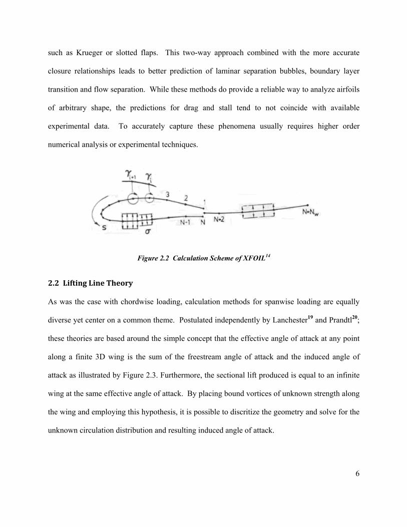
A similar yet more accurate method proposed by Drela14,15,16 uses a two-way coupled approach.
This accounts for the effects of both boundary layer and wake on the flow. This is accomplished
by placing both surface bound vortices and surface/wake bound source elements as shown in
Figure 2.2. Several engineering level codes are available which utilize the two-way coupled
approach, namely XFOIL17 and MSES18 , the latter being applicable to multi-element airfoils
6
such as Krueger or slotted flaps. This two-way approach combined with the more accurate
closure relationships leads to better prediction of laminar separation bubbles, boundary layer
transition and flow separation. While these methods do provide a reliable way to analyze airfoils
of arbitrary shape, the predictions for drag and stall tend to not coincide with available
experimental data. To accurately capture these phenomena usually requires higher order
numerical analysis or experimental techniques.
Figure 2.2 Calculation Scheme of XFOIL14
2.2 LiftingLineTheory
As was the case with chordwise loading, calculation methods for spanwise loading are equally
diverse yet center on a common theme. Postulated independently by Lanchester19 and Prandtl20;
these theories are based around the simple concept that the effective angle of attack at any point
along a finite 3D wing is the sum of the freestream angle of attack and the induced angle of
attack as illustrated by Figure 2.3. Furthermore, the sectional lift produced is equal to an infinite
wing at the same effective angle of attack. By placing bound vortices of unknown strength along
the wing and employing this hypothesis, it is possible to discritize the geometry and solve for the
unknown circulation distribution and resulting induced angle of attack.

7
Figure 2.3 Lanchester/Prandtl Hypothesis7
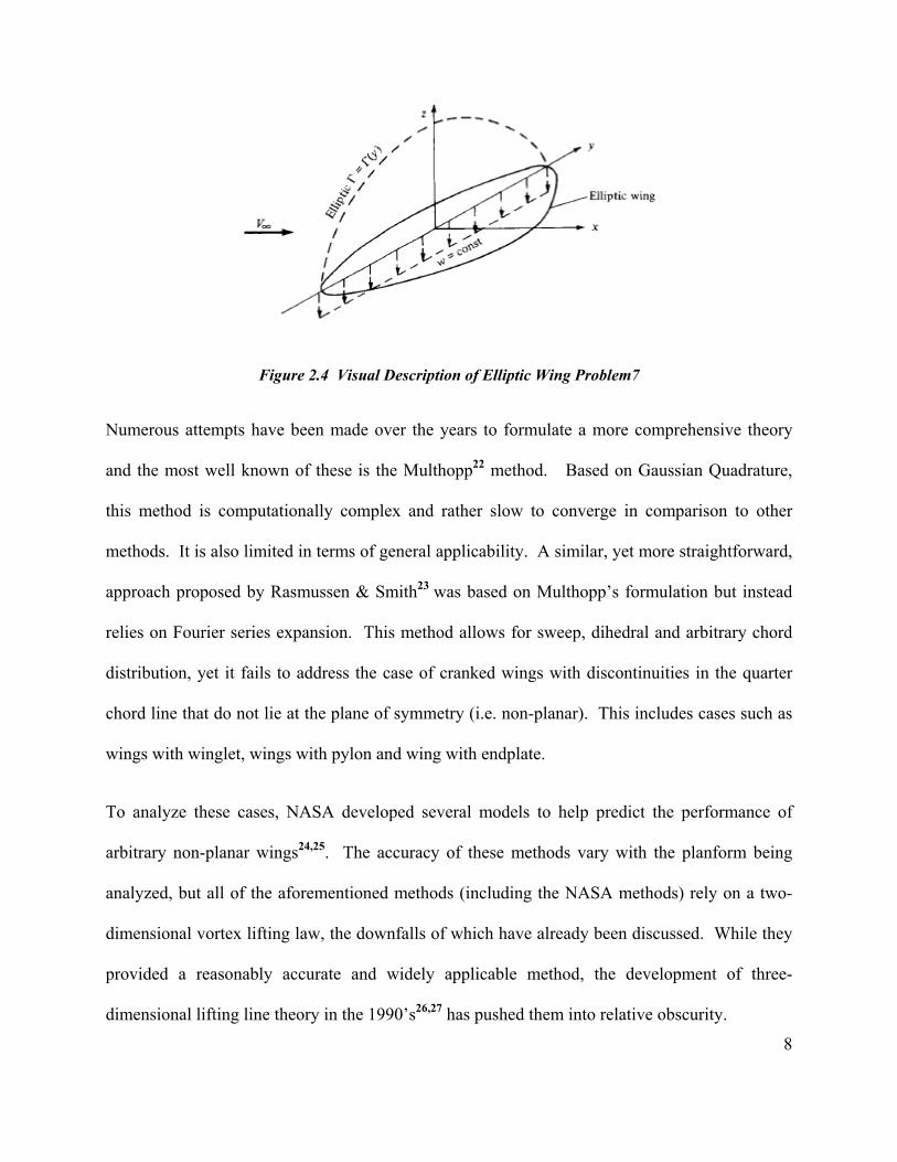
Prandtl successfully applied this theory to the elliptic wing problem illustrated in Figure 2.4.
Through some intuitive reasoning he was able to derive a closed form solution that is found in
most aerodynamic textbooks7,8,9. However, this solution is a rather unique case and closed form
solutions do not exist for any other geometry. A more generalized approach is usually found in
these same texts which allows for non-elliptic chord distributions, wing incidence and twist as
well as variation in airfoil geometry.
Commonly called the general lift distribution method, it is only applicable to wings with no
sweep or dihedral. Since most modern lifting surfaces exhibit one or both of these geometric
properties, this method is far from generic. Typically, the failure of the ‘General Lift
Distribution’ method is attributed to its inability to predict spanwise flow; however, this has been
shown to be false21 with the application of a three-dimensional lifting law rather than the two
dimensional law used in the general method. In reality, the pitfall of these methods can be traced
to their neglect of the influence of a bound vortex on itself27.
8
Figure 2.4 Visual Description of Elliptic Wing Problem7
Numerous attempts have been made over the years to formulate a more comprehensive theory
and the most well known of these is the Multhopp22 method. Based on Gaussian Quadrature,
this method is computationally complex and rather slow to converge in comparison to other
methods. It is also limited in terms of general applicability. A similar, yet more straightforward,
approach proposed by Rasmussen & Smith23 was based on Multhopp’s formulation but instead
relies on Fourier series expansion. This method allows for sweep, dihedral and arbitrary chord
distribution, yet it fails to address the case of cranked wings with discontinuities in the quarter
chord line that do not lie at the plane of symmetry (i.e. non-planar). This includes cases such as
wings with winglet, wings with pylon and wing with endplate.
To analyze these cases, NASA developed several models to help predict the performance of
arbitrary non-planar wings24,25. The accuracy of these methods vary with the planform being
analyzed, but all of the aforementioned methods (including the NASA methods) rely on a two-
dimensional vortex lifting law, the downfalls of which have already been discussed. While they
provided a reasonably accurate and widely applicable method, the development of three-
dimensional lifting line theory in the 1990’s26,27 has pushed them into relative obscurity.

9
This modernized lifting line theory utilizes a three-dimensional vortex lifting law which can
account for spanwise flow, non-planar effects and self induced velocity. While mathematically
this method is applicable to the general case, solutions of the published models exhibit
singularities that are caused by discontinuities chord line. These discontinuities cause a local
shift in locus of aerodynamic centers which are normally assumed to be located at the quarter-
chord position for straight wings. This effect is well known and has been documented in
countless experiments including the work of Weber & Brebner28 as well as Hall & Rogers29.
To account for this shift in aerodynamic center in swept wings, the tangent approximation can be
used. Presented by Küchemann30 as part of a lifting-line theory for swept wings, the tangent
approximation has been shown to agree quite well with experimental data. However, the method
is only applicable to planar swept wings with no kinks in the quarter-chord line. The impact of a
multi-paneled (or cranked) wing and the effects of dihedral are not accounted for limiting the
usefulness of the tangent approximation. Considerable effort was expended to locate an all
encompassing aerodynamic center shift theory that can be applied to the arbitrary case, but none
was found. Thankfully, the tangent approximation is simple enough that extension to the general
case is quite easy and will be discussed in subsequent sections. Unfortunately, it will also be
shown that despite mitigating the singularity, the application of the tangent approximate has
unwanted consequences on the predicted spanwise loading of a given lifting surface.
2.3 VortexLatticeMethod
Similar in methodology to Lifting Line Theory, the Vortex Lattice Method (VLM) allows for a
solution which yields both spanwise and chordwise loading. This is accomplished by placing a
series of horseshoe vortices along the wing in both the span and chordwise directions effectively
10
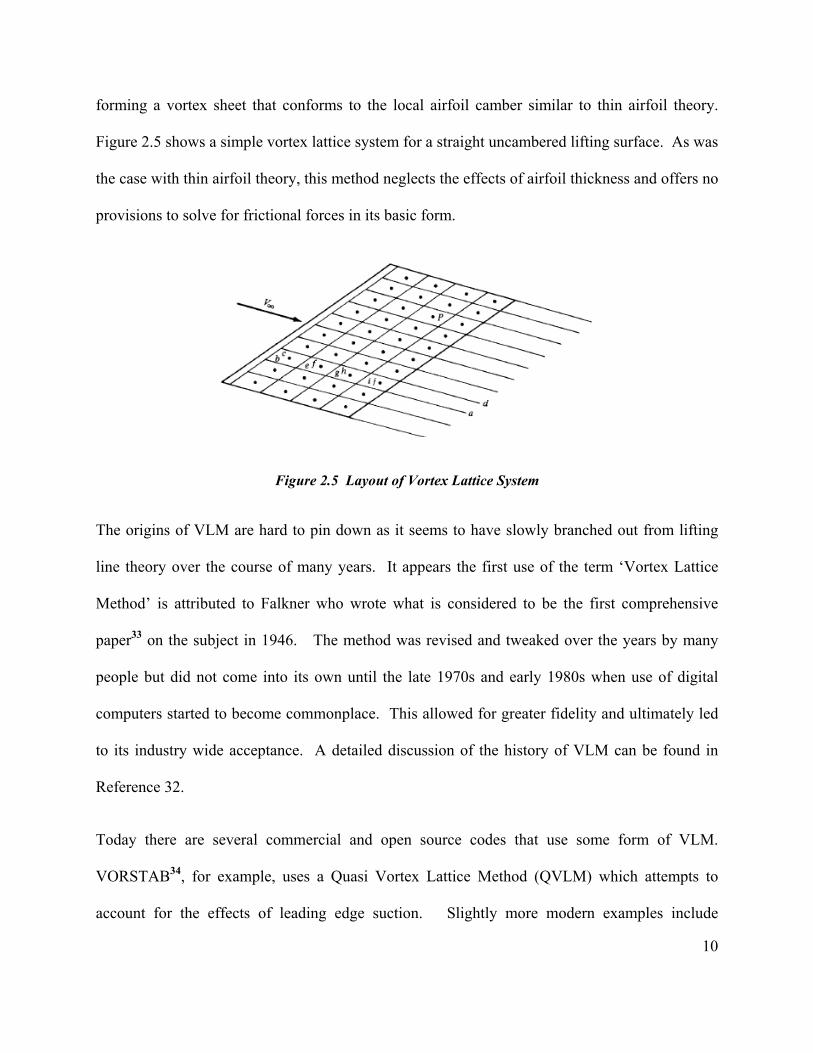
forming a vortex sheet that conforms to the local airfoil camber similar to thin airfoil theory.
Figure 2.5 shows a simple vortex lattice system for a straight uncambered lifting surface. As was
the case with thin airfoil theory, this method neglects the effects of airfoil thickness and offers no
provisions to solve for frictional forces in its basic form.
Figure 2.5 Layout of Vortex Lattice System
The origins of VLM are hard to pin down as it seems to have slowly branched out from lifting
line theory over the course of many years. It appears the first use of the term ‘Vortex Lattice
Method’ is attributed to Falkner who wrote what is considered to be the first comprehensive
paper33 on the subject in 1946. The method was revised and tweaked over the years by many
people but did not come into its own until the late 1970s and early 1980s when use of digital
computers started to become commonplace. This allowed for greater fidelity and ultimately led
to its industry wide acceptance. A detailed discussion of the history of VLM can be found in
Reference 32.
Today there are several commercial and open source codes that use some form of VLM.
VORSTAB34, for example, uses a Quasi Vortex Lattice Method (QVLM) which attempts to
account for the effects of leading edge suction. Slightly more modern examples include
11
Tornado35 and AVL36 which have user friendly Graphical User Interfaces (GUI’s) but yield
essentially similar results. While these codes are quite good at analyzing arbitrary lifting
surfaces for lift, pitching moment and induced drag, they make no attempt to address the impact
of frictional forces or airfoil thickness and cannot predict stall or flow separation.
2.4 3DPanelMethods
The relationship of thin airfoil theory and the airfoil panel methods is very much analogous to
the relationship of VLM and 3DP. Where VLM relies on vortices bound to the camber line, 3DP
methods place vortices on the lifting surface and solves for the resulting potential flow. There
are a couple of approaches to this but they all solve some form of the Euler equation.
A linearized form of the Euler equation common to fluid dynamics is known as the Prandtl-
Glauert equation and can be found in most aerodynamic textbooks7,8,9. This is often described as
the origin of modern Computational Fluid Dynamics (CFD), but this is really not the case. The
Prandtl-Glauert equation solves for potential flow, a condition which can never truly exist in
nature, whereas modern CFD techniques try to solve the continuum mechanics equations. This
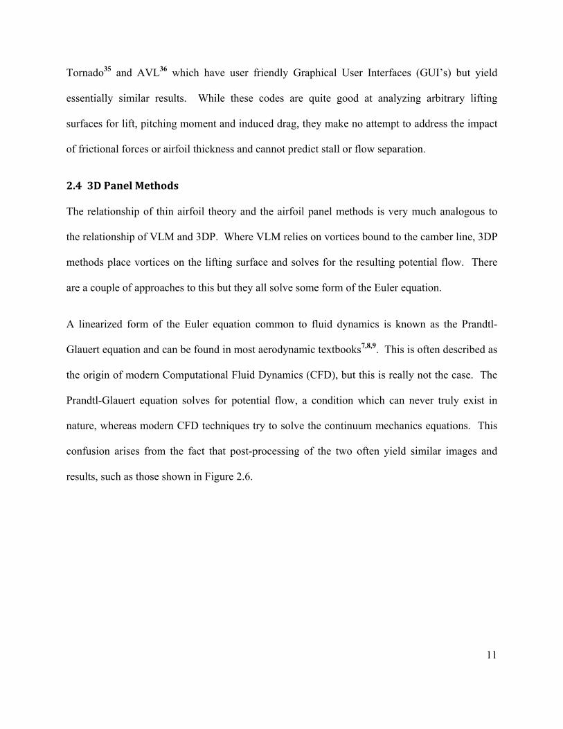
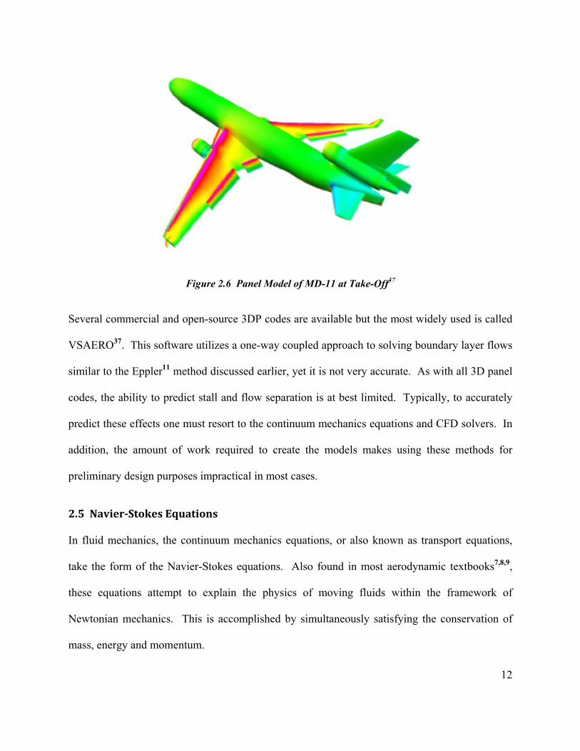
confusion arises from the fact that post-processing of the two often yield similar images and
results, such as those shown in Figure 2.6.
12
Figure 2.6 Panel Model of MD-11 at Take-Off37
Several commercial and open-source 3DP codes are available but the most widely used is called
VSAERO37. This software utilizes a one-way coupled approach to solving boundary layer flows
similar to the Eppler11 method discussed earlier, yet it is not very accurate. As with all 3D panel
codes, the ability to predict stall and flow separation is at best limited. Typically, to accurately
predict these effects one must resort to the continuum mechanics equations and CFD solvers. In
addition, the amount of work required to create the models makes using these methods for
preliminary design purposes impractical in most cases.
2.5 Navier‐StokesEquations
In fluid mechanics, the continuum mechanics equations, or also known as transport equations,
take the form of the Navier-Stokes equations. Also found in most aerodynamic textbooks7,8,9,
these equations attempt to explain the physics of moving fluids within the framework of
Newtonian mechanics. This is accomplished by simultaneously satisfying the conservation of
mass, energy and momentum.
13
Closed form solutions of these equations are only possible for the simplest of cases, such as
Couette flow, channel flow or laminar pipe flow38. Solutions for the general case require
numerical techniques which can be quite involved. Turbulence models which describe the
higher order terms of the Navier-Stokes equations are almost always necessary to solve these
types of problems38. Unfortunately, no single turbulence model adequately predicts this
phenomenon in all types of flow environments or scenarios. This is due in part to the fact that
these models attempt to explain turbulence that occurs at various scales within all moving fluids,
but are usually limited to some narrow band of that range. For example, the microscopic eddies
created by turbulent mixing of the boundary layer are not adequately explained by turbulence
models which are capable of describing large eddies like those found in the wake of a boat or an
airplane.
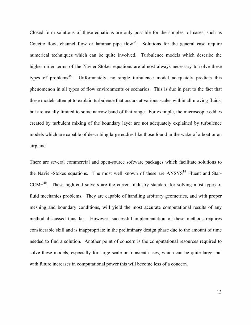
There are several commercial and open-source software packages which facilitate solutions to
the Navier-Stokes equations. The most well known of these are ANSYS39 Fluent and Star-
CCM+40. These high-end solvers are the current industry standard for solving most types of
fluid mechanics problems. They are capable of handling arbitrary geometries, and with proper
meshing and boundary conditions, will yield the most accurate computational results of any
method discussed thus far. However, successful implementation of these methods requires
considerable skill and is inappropriate in the preliminary design phase due to the amount of time
needed to find a solution. Another point of concern is the computational resources required to
solve these models, especially for large scale or transient cases, which can be quite large, but
with future increases in computational power this will become less of a concern.

14
Figure 2.7 Example of High Fidelity CFD Results40
2.6 MIAReXandXFLR5
One particularly useful tool which is appropriate for preliminary design is known as XFLR541.
This program contains several analysis tools ranging from airfoil analysis to 3D panel methods
and is popular in universities all over the world due to its user friendly interface. It is separated
into four main analysis types; airfoil analysis, lifting-line theory, VLM and a 3D panel method.
The airfoil analysis methods utilized in XFLR5 are identical to those found in XFOIL17 with
many of the same geometric design and post-processing features.
The lifting line theory used is from an antiquated NACA model42 for which the original
formulation is not applicable to cranked or non-planar cases. This is employed within the
framework of MIAReX43, a computational approach designed to distribute pressure forces along
a 3D surface from either experimental or computational airfoil data. It is remarkably similar in
formulation to the pressure distribution method presented in the original formulation1 of the
proposed method, yet it is entirely unclear how this is extended to the general case since
documentation on this software leaves much to be desired.
15
The exact formulations of the VLM and 3DP codes included in XFLR5 are also unknown, again
due to poor documentation of the software, though the VLM and 3DP code include options for
viscous effects and ground effect which suggests more sophisticated models. Unfortunately,
they are very temperamental and very rarely if ever allow for the solution to converge.
Extensive use of this software will be made for comparative purposes without employing these
troublesome viscous flow options.
2.7 WindTunnelTesting
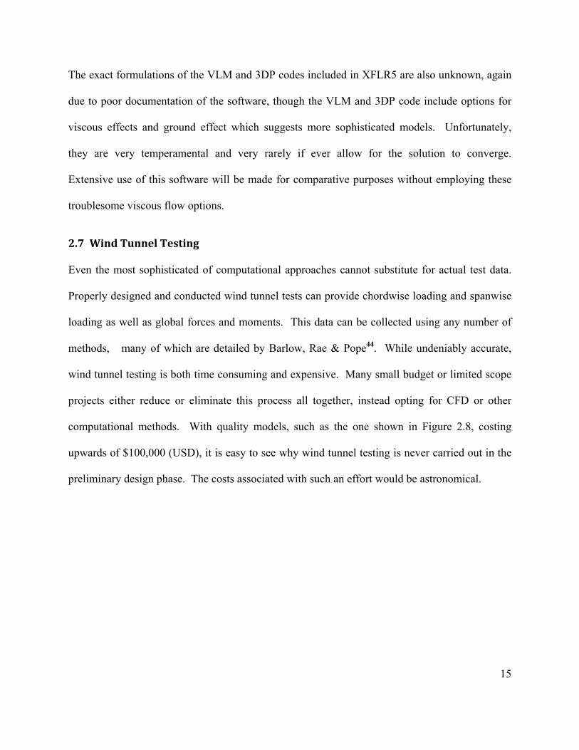
Even the most sophisticated of computational approaches cannot substitute for actual test data.
Properly designed and conducted wind tunnel tests can provide chordwise loading and spanwise
loading as well as global forces and moments. This data can be collected using any number of
methods, many of which are detailed by Barlow, Rae & Pope44. While undeniably accurate,
wind tunnel testing is both time consuming and expensive. Many small budget or limited scope
projects either reduce or eliminate this process all together, instead opting for CFD or other
computational methods. With quality models, such as the one shown in Figure 2.8, costing
upwards of $100,000 (USD), it is easy to see why wind tunnel testing is never carried out in the
preliminary design phase. The costs associated with such an effort would be astronomical.

16
Figure 2.8 Example of High Quality Wind Tunnel Model45
2.8 Conclusions
As has been shown, the methods for determining distributed aerodynamic loads on lifting
surfaces take a variety of forms. They range from being simple enough that they can be solved
by hand to requiring massive super computers and hours of computational time to converge.
Depending on the application and current design phase, one or more may be appropriate, yet in
the preliminary design phase few solutions exist which are arbitrary and easily understood, let
alone applied. It will be shown that by combining some of the more simple loading theories, a
more complex understanding can be developed and incorporated into the preliminary design
process which rivals that of the higher fidelity methods in some limited respects.
17
3. Theoretical Development
This section summarizes the theoretical development of the proposed method. A general
overview is offered followed by formulations of the various components that make up the
method and concludes with a discussion of the calculation of forces, moments and their
respective coefficients.
3.1 Overview
The methodology outlined in the following sections describes a process by which planforms of
arbitrary shape can be analyzed in a quick and effective manner. By themselves, the methods
employed are easy to understand, but when combined into a cohesive theory, they provide a
powerful computational tool for aerodynamicists and aircraft designers. The theory centers on
the use of a lifting line method, solutions to which provide angle of attack distributions that are
used to generate local lift and drag data as well as pressure and frictional force distributions.
This can come from any resource (computational or experimental) capable of resolving
chordwise loading, yet the accuracy of the airfoil methods directly impact the accuracy of the
final results resulting in a trade-off between flexibility and accuracy.
While wind tunnel testing provides accurate and reliable data, the expense and lack of
comprehensive databases of experimental results make application to the general case
impossible. However, by utilizing any one of the numerical approaches discussed in Section 2.1,
almost any airfoil section can be analyzed with varying degrees of accuracy. At a minimum, the
airfoil pressure distribution and lift coefficient at several angles of attack and comparable
Reynolds number must be known. If skin friction distributions or drag and moment coefficients
are also known, additional post processing is possible.
18
3.2 ChordLoading
To achieve the objectives stated in Section 1.1, XFOIL v6.917 has been selected as the preferred
analysis tool. It is capable of analyzing airfoils of arbitrary shape over a reasonable range of
angle of attack and Mach number. The geometry modification routines contained within XFOIL
allow for plain control surface deflections (i.e. aileron, plain flap, flaperon, etc…), further
extending the applicability of the software, but it unfortunately does not provide a complete
picture. By making some simple assumptions and applying the Viterna method47 for
extrapolating airfoil data, it is possible to fill in the gaps and obtain a more complete answer.
The two-way coupled analysis in XFOIL17 is discussed in detail by Drela14,16 so only the basic
equations and governing principles are discussed here. What makes XFOIL a two-way coupled
analysis is the fact that the potential flow calculations account for boundary layer and wake
effects by use of additional source distributions as depicted by Figure 2.2. The stream function
governing the potential solution is given by Equation 114 and is the superposition (or sum) of the
freestream stream function and the stream functions of the surface bound vortices and
surface/wake bound source elements.
1 1, ln
2 2xyx y u y v x s r s ds s s ds (1)
In turn, the equations governing the viscous flow are dominated by a compressible version of the
Von Kármán Momentum Integral equation, shown below in Equation 214. However, this
requires an accompanying shape parameter integral that relates the shape of the boundary layer
to the external potential flow and is given by Equation 314.

19
2(2 )2
fee
e
cd duH M
d u d
(2)
*
*** * *2 1 2
2fe
De
cdH duH H H C H
d u d
(3)
A third governing equation for the viscous flow equations is also required, yet its form and
function vary depending on whether the boundary layer is laminar or turbulent. Prior to
transition when the boundary layer is still considered laminar, this takes the form of the shear
stress lag equation given by Equation 414 and is used until the amplification factor, n , equals a
user specified value, critn , indicating transition.
Re,
Re k k
dn dn dH H
d d d
(4)
After transition, the boundary layer is considered turbulent and Equation 4 is replaced by the
maximum shear stress rate equation given by Equation 514.
2
*
4 1 15.6 2
3 2 6.7EQ
f k et t
k e
cdC H duC C
C d H u d
(5)
The systems of linear ODE’s formed by Equations 2 through 5 contain a total of ten unknowns
requiring seven separate closure relationships. These are empirical formulas derived from a
combination of solutions to the Falkner-Skan equation and experimental observations14. These
are documented in detail by Drela & Giles16, but the general relationships of the variables can be
separated into shape parameter functions (Equation 6) which relate various features of the
20
boundary layer to each other and coefficient functions (Equation 7) which relate the features of
the boundary layer to its quantifiable values.
*
**
*
( , )
( , Re , )Shape Parameters
( , )
( , , )
k e
k e
k e
S k
H f H M
H f H M
H f H M
U f H H H
(6)
*
*, , ,
Coefficeints , Re ,
( , , )
EQ k S
f k e
S fD
C f H H H U
c f H M
C f U C c
(7)
Solutions are obtained by coupling Equation 1 with Equations 2 through 7 as follows. To begin,
an initial estimate of the stream function (Equation 1) is made assuming inviscid potential flow
with no source distribution (i.e. 0 ). This yields vortex panel strengths along the airfoil
which are converted to incompressible velocity and pressure coefficient using Equations 8 and
914. If desired, corrections for compressibility can be made using the Kármán-Tsien correction
(Equations 10 through 13) 14. However, these equations are only applicable for freestream Mach
numbers up to about 0.5 where local surface velocity can spike into the supersonic regieme.
The drag calculations also make no provisions for wave drag which can dominate the total
planform drag in the transonic regieme (around Mach 0.7).
ie ju (8)
21
ip jc (9)
21
12
i
i
pp
pc c c
cc
c
(10)
2
1
1
ei ce
eic
uu
u
U
(11)
21c M (12)
2
21
c
c
M
(13)
Using the initial estimate for the potential flow that rolls out of either Equation 8 or 11, the
corresponding boundary layer properties can be calculated using Equations 2 through 7. From
these results the mass deficit caused by the boundary layer is found from Equation 1414 and
applied to Equation 1. The process then starts again, this time accounting for the influence of
the boundary layer and wake on the potential function.
*e
du
d
(14)
The potential function which results from the recalculation is used to determine the velocity and
surface pressure coefficient along the airfoil surface and wake via Equations 1514 and 9,
respectively. This is followed by compressibility corrections (if desired) via the Kármán-Tsien
relationship given by Equations 10 through 13.

22
for airfoil
ˆ for wakei
jeu
n
(15)
The boundary layer properties are again estimated using Equations 2 through 7 and the process is
repeated until the predicted source and vortex strengths converge to within some acceptable
tolerance. This results in pressure coefficient and skin friction coefficient distributions as well as
boundary layer properties along the airfoil surface. XFOIL assumes that the contribution of
friction to lift and pitching moment is negligible and calculates the corresponding lift and
moment coefficients using Equations 1646 and 1746.
l pc c dx (16)
/4
0.25cm p pc c x dx c ydy (17)
Since friction cannot be neglected when considering drag, XFOIL17 calculates total profile drag
using the Squire-Young formula given by Equation 1846. The contribution of friction is
determined by integrating the skin friction coefficient around the airfoil as shown by Equation
1946. Unfortunately, a similar calculation of pressure drag is not possible as it is swamped by
numerical noise. Instead, the pressure drag is calculated by assessing the difference between
profile drag and skin friction drag as shown by Equation 2046.
5
2
2
wake
wake
H
ed
uc
U
(18)
fd fc c dx (19)
23
p fd d dc c c (20)
Where;
cos sinx x y (21)
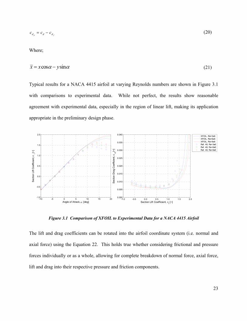
Typical results for a NACA 4415 airfoil at varying Reynolds numbers are shown in Figure 3.1
with comparisons to experimental data. While not perfect, the results show reasonable
agreement with experimental data, especially in the region of linear lift, making its application
appropriate in the preliminary design phase.
Figure 3.1 Comparison of XFOIL to Experimental Data for a NACA 4415 Airfoil
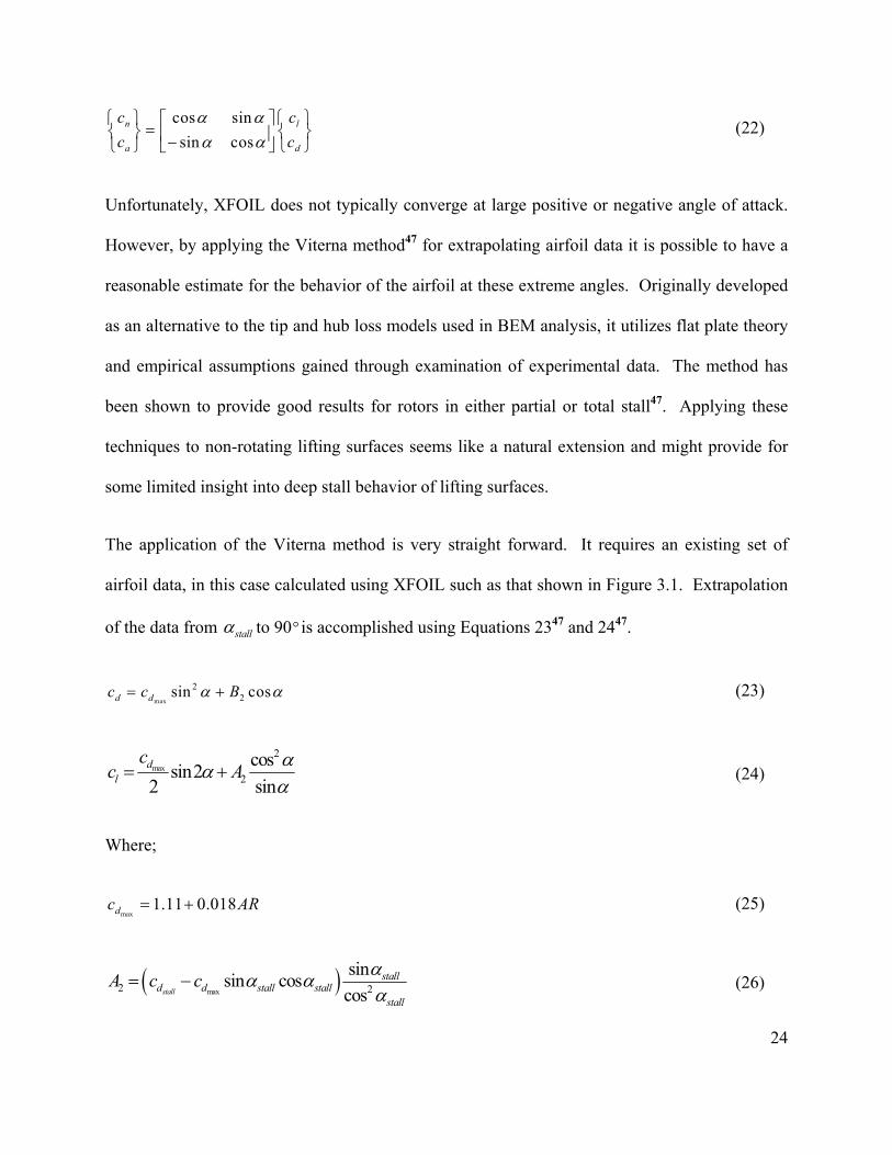
The lift and drag coefficients can be rotated into the airfoil coordinate system (i.e. normal and
axial force) using the Equation 22. This holds true whether considering frictional and pressure
forces individually or as a whole, allowing for complete breakdown of normal force, axial force,
lift and drag into their respective pressure and friction components.
-10 -5 0 5 10 15 20-1.0
-0.5
0.0
0.5
1.0
1.5
2.0
Angle of Attack, [deg]
Sec
tion
Lift
Co
effic
ien
t, c
l [~]
-1.0 -0.5 0.0 0.5 1.0 1.5 2.00.000
0.005
0.010
0.015
0.020
0.025
0.030
0.035
0.040
Section Lift Coefficient, cl [~]
Sec
tion
Dra
g C
oeffi
cie
nt, c
d [~]
XFOIL, Re=3e6XFOIL, Re=6e6XFOIL, Re=9e6Ref. 48, Re=3e6Ref. 48, Re=6e6Ref. 48, Re=9e6
24
cos sin
sin cosn l
a d
c c
c c
(22)
Unfortunately, XFOIL does not typically converge at large positive or negative angle of attack.
However, by applying the Viterna method47 for extrapolating airfoil data it is possible to have a
reasonable estimate for the behavior of the airfoil at these extreme angles. Originally developed
as an alternative to the tip and hub loss models used in BEM analysis, it utilizes flat plate theory
and empirical assumptions gained through examination of experimental data. The method has
been shown to provide good results for rotors in either partial or total stall47. Applying these
techniques to non-rotating lifting surfaces seems like a natural extension and might provide for
some limited insight into deep stall behavior of lifting surfaces.
The application of the Viterna method is very straight forward. It requires an existing set of
airfoil data, in this case calculated using XFOIL such as that shown in Figure 3.1. Extrapolation
of the data from stall to 90is accomplished using Equations 2347 and 2447.
max
22sin cosd dc c B (23)
max
2
2
cossin2
2 sind
l
cc A
(24)
Where;
max1.11 0.018dc AR (25)
max2 2
sinsin cos
cosstall
stalld d stall stall
stall
A c c
(26)

25
max
2
2
sin
cosstalld d stall
stall
c cB
(27)
The aspect ratio term of Equation 25 is a carryover from the BEM application where finite blade
length affects the flat plate assumption. This can either be the aspect ratio of the lifting surface
or a recommended default value of 10. The actual value makes little impact on the final results.
For α > 90˚ and α < αmin the calculated values are reflected. A scaling factor of 0.7 is applied to
the reflected lift values to account for cambered airfoils. If the airfoils are uncambered the
scaling factor is assumed to be 1.0 and the left hand reflection point shifts from αmin to α = 0˚.
Figure 3.2 shows the results of the Viterna method applied to a NACA 4415 airfoil.
Figure 3.2 Airfoil Data Extrapolated via Viterna Method, NACA 4415 at Re=3e6 and AR=10
The Viterna method does not make any provisions for pressure or skin friction distributions;
however, by making a few simple assumptions it is possible to provide a reasonable estimate
which meets the results predicted using the Viterna method. From examining a plot of the
contributions of pressure and friction to axial force, it is clear that it is dominated by pressure as
evidenced by Figure 3.3. Furthermore, the variation in the axial friction force tends to be quite
-2
-1
0
1
2
Sec
tion
Lift
Co
effic
ien
t, c
l [~]
-180 -150 -120 -90 -60 -30 0 30 60 90 120 150 1800
0.5
1
1.5
Angle of Attack, [deg]Sec
tion
Dra
g C
oeffi
cie
nt, c
d [~]
Extent of XFOIL Data
Extent of XFOIL Data

26
small and can be assumed to be constant and equal to the mean of the available values. Keeping
the assumption in place that the frictional contribution to lift is negligible, it is possible to apply
the inverse of Equation 22 to decompose the extrapolated axial force, normal force, lift and drag
into their respective pressure and frictional contributions.
Figure 3.3 Contribution of Pressure and Friction to Axial Force for NACA 4415 at Re=3e6
From the extrapolated coefficients, it is possible to assign pressure and skin friction distributions
based on the assumption of simple separated flat plate flow as illustrated by Figure 3.4. While
not an accurate representation of the true physics, it provides a reasonable estimate for early in
the design process. What this implies is that the suction surface of the flat plate experiences
completely separated flow resulting in ambient pressure. This requires the pressure surface to
produce all of the normal pressure forces on the plate. In addition both surfaces of the plate
experience constant skin friction of equal magnitude and both pressure and frictional
distributions must integrate via Equations 28 and 29 to match the extrapolated and decomposed
Viterna results for normal pressure and axial friction forces.
-10 -5 0 5 10 15 20-0.6
-0.5
-0.4
-0.3
-0.2
-0.1
0.0
0.1
Angle of Attack, [deg]
Sec
tion
Axi
al F
orce
Coe
ffici
ent
, ca [~
]
PressureFriction
27
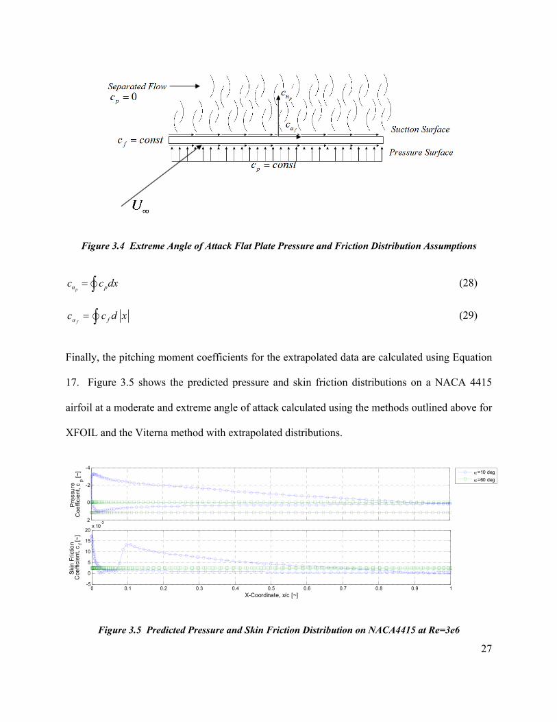
Figure 3.4 Extreme Angle of Attack Flat Plate Pressure and Friction Distribution Assumptions
pn pc c dx (28)
fa fc c d x (29)
Finally, the pitching moment coefficients for the extrapolated data are calculated using Equation
17. Figure 3.5 shows the predicted pressure and skin friction distributions on a NACA 4415
airfoil at a moderate and extreme angle of attack calculated using the methods outlined above for
XFOIL and the Viterna method with extrapolated distributions.
Figure 3.5 Predicted Pressure and Skin Friction Distribution on NACA4415 at Re=3e6
-4
-2
0
2
Pre
ssu
re
Coe
ffici
ent
, cp [~
]
0 0.1 0.2 0.3 0.4 0.5 0.6 0.7 0.8 0.9 1-5
0
5
10
15
20x 10
-3
X-Coordinate, x/c [~]
Ski
n F
rict
ion
Coe
ffici
ent
, cf [~
]
=10 deg
=60 deg

28
3.3 SpanLoading
The lifting line theory selected for the proposed method is the Phillips27 method and is based on
the 3D vortex lifting law. It is a simple and elegant method capable of providing extremely
useful results. The theory centers on placing a series of discrete horseshoe vorticies along the
wing and equating the lift calculated using the 3D vortex lifting law with the section lift
calculated using the methods outlined in Section 3.2. Figure 3.6 shows a typical wing vortex
system. Essentially, this amounts to a vortex-lattice method constrained to only one chordwise
element with the effects of camber, flap deflection and airfoil thickness being adequately
modeled using airfoil data.
Figure 3.6 Example Wing Vortex System
When applied to a differential segment containing the bound portion of a horseshoe vortex, the
3D vortex lifting law takes the form of Equation 3027. This is equated to the lift force created on
that differential element of the wing based on the available airfoil data via Equation 31.
29
v
F V dv df V d (30)
21
2 ldf V c A
(31)
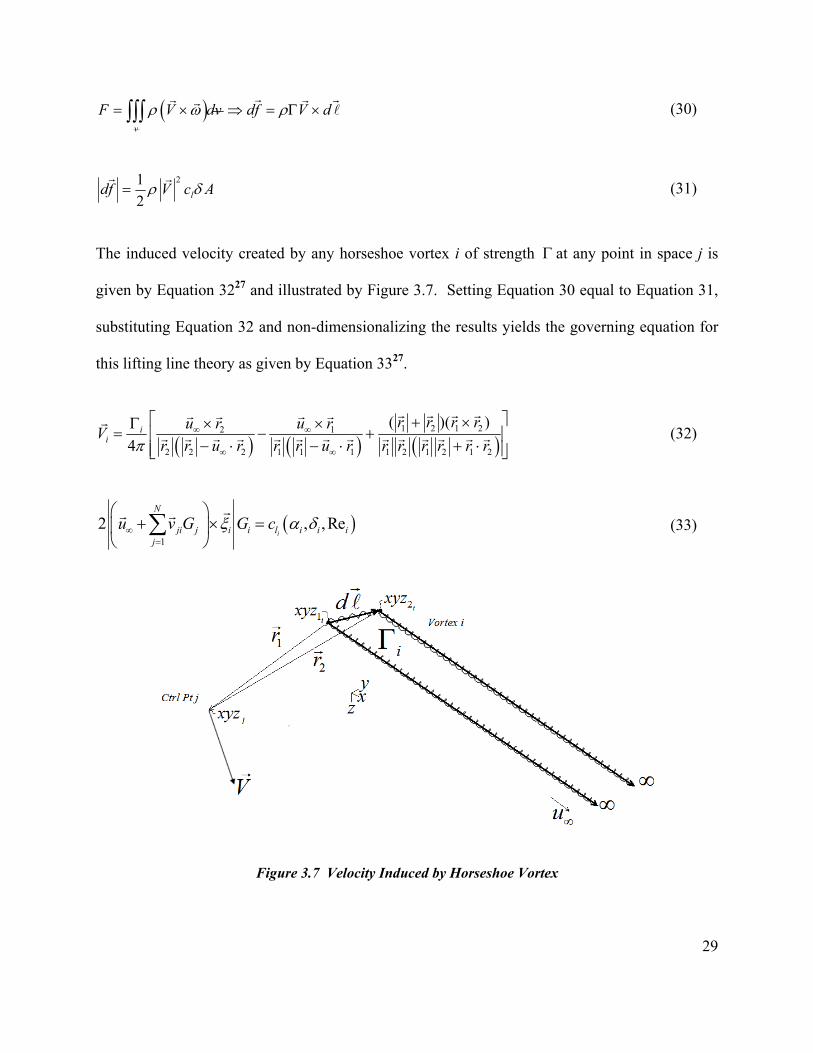
The induced velocity created by any horseshoe vortex i of strength at any point in space j is
given by Equation 3227 and illustrated by Figure 3.7. Setting Equation 30 equal to Equation 31,
substituting Equation 32 and non-dimensionalizing the results yields the governing equation for
this lifting line theory as given by Equation 3327.
1 2 1 22 1
2 2 2 1 1 1 1 2 1 2 1 2
( )( )
4i
i
r r r ru r u rV
r r u r r r u r r r r r r r
(32)
1
2 , ,Rei
N
ji j i i l i i ij
u v G G c
(33)
Figure 3.7 Velocity Induced by Horseshoe Vortex

30
The remaining terms of Equation (33) are defined as follows:
Uu
U
(34)
i i
dc
A
(35)
ii
i
Gc U
(36)
11
1
tani
i
N
ji j nj
i N
ji j aj
u v G u
u v G u
(37)
, 2 1 124i
j i
cv v v v
(38)
Where;
1
11 1 1
u rv
r r u r
(39)
2
22 2 2
u rv
r r u r
(40)
1 2 1 212
1 2 1 2 1 2
0 for i = j
( )( ) for i j
r r r rv
r r r r r r
(41)
31
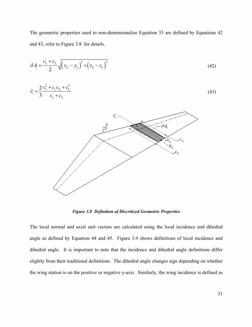
The geometric properties used to non-dimensionalize Equation 33 are defined by Equations 42
and 43, refer to Figure 3.8 for details.
2 21 22 1 2 12
i i
i i i ii
c cA y y z z
(42)
2 21 1 2 2
1 2
2
3i i i i
i i
i
c c c cc
c c
(43)
Figure 3.8 Definition of Discritized Geometric Properties
The local normal and axial unit vectors are calculated using the local incidence and dihedral
angle as defined by Equation 44 and 45. Figure 3.9 shows definitions of local incidence and
dihedral angle. It is important to note that the incidence and dihedral angle definitions differ
slightly from their traditional definitions. The dihedral angle changes sign depending on whether
the wing station is on the positive or negative y-axis. Similarly, the wing incidence is defined as
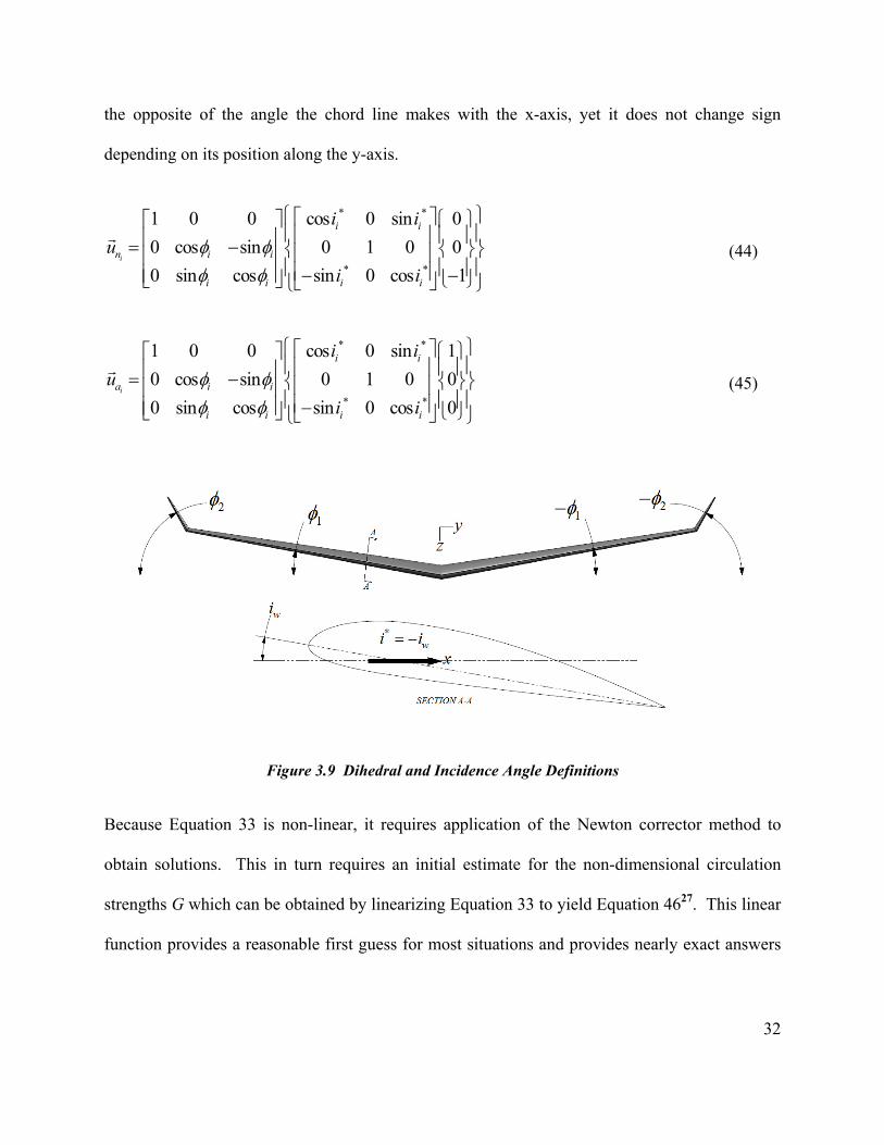
32
the opposite of the angle the chord line makes with the x-axis, yet it does not change sign
depending on its position along the y-axis.
* *
* *
1 0 0 cos 0 sin 0
0 cos sin 0 1 0 0
0 sin cos sin 0 cos 1i
i i
n i i
i i i i
i i
u
i i
(44)
* *
* *
1 0 0 cos 0 sin 1
0 cos sin 0 1 0 0
0 sin cos sin 0 cos 0i
i i
a i i
i i i i
i i
u
i i
(45)
Figure 3.9 Dihedral and Incidence Angle Definitions
Because Equation 33 is non-linear, it requires application of the Newton corrector method to
obtain solutions. This in turn requires an initial estimate for the non-dimensional circulation
strengths G which can be obtained by linearizing Equation 33 to yield Equation 4627. This linear
function provides a reasonable first guess for most situations and provides nearly exact answers
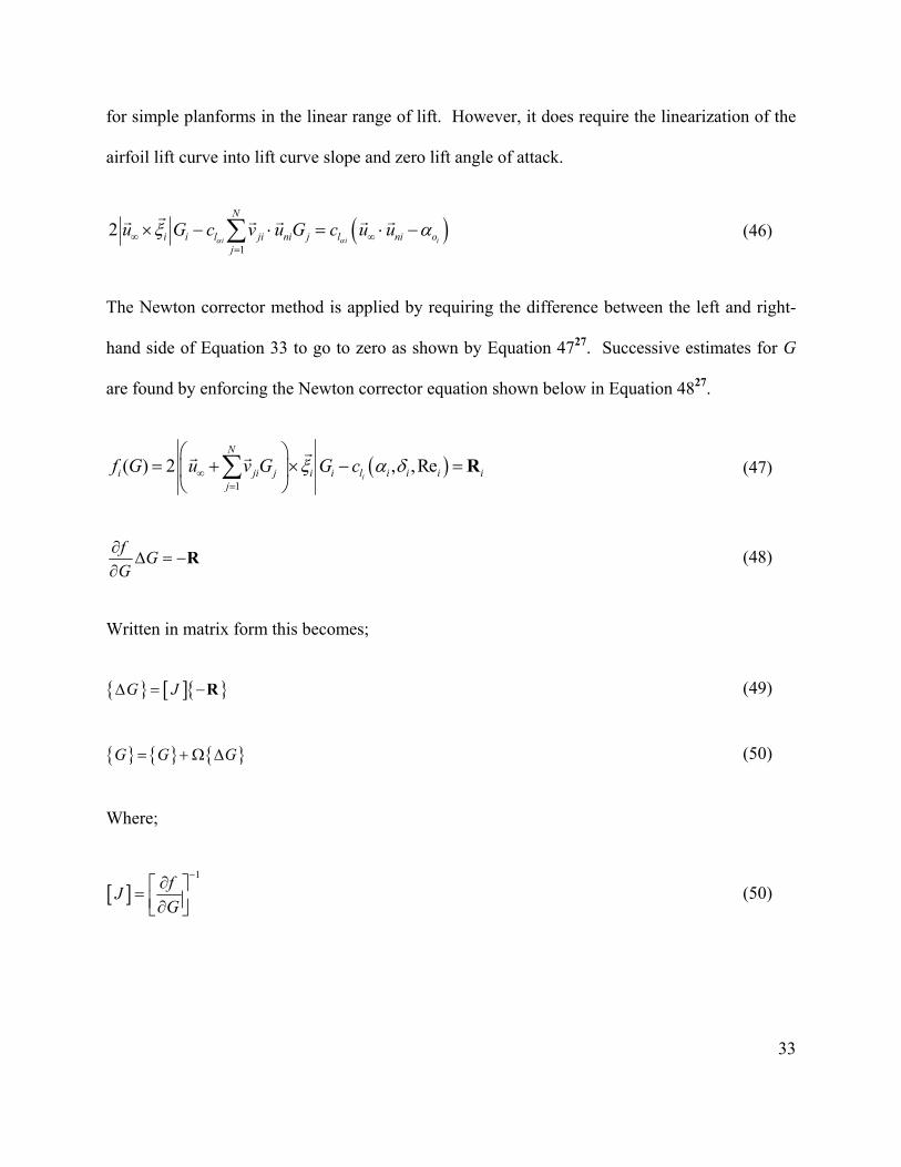
33
for simple planforms in the linear range of lift. However, it does require the linearization of the
airfoil lift curve into lift curve slope and zero lift angle of attack.
1
2i i i
N
i i l ji ni j l ni oj
u G c v u G c u u
(46)
The Newton corrector method is applied by requiring the difference between the left and right-
hand side of Equation 33 to go to zero as shown by Equation 4727. Successive estimates for G
are found by enforcing the Newton corrector equation shown below in Equation 4827.
1
( ) 2 , ,Rei
N
i ji j i i l i i i ij
f G u v G G c
R
(47)
fG
G
R (48)
Written in matrix form this becomes;
G J R (49)
G G G (50)
Where;
1
fJ
G
(50)
34
2 2
2 2
2
22
i
i
i ji i ai ji ni ni ji aili
i i ai ni
ij
i ji i ai ji ni ni ji aili i
i i ai ni
w v v v u v v ucG for i j
w v vJ
w v v v u v v ucw G for i j
w v v
(51)
1
N
i ji j ij
w u v G
(52)
1
N
ni ji j nij
v u v G u
(53)
1
N
ai ji j aij
v u v G u
(54)
Solutions are found by getting an initial estimate for G from Equation 46. Written in matrix
form, this quickly surrenders to matrix inversion as shown by Equations 55 through 57.
,
2
i
i
i l ji ni i
i j
l ji ni j
u c v u G for i j
c v u G for i j
(55)
i ii l ni oH c u u
(56)
1G H
(57)
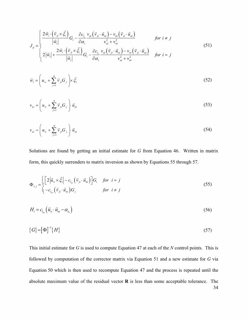
This initial estimate for G is used to compute Equation 47 at each of the N control points. This is
followed by computation of the corrector matrix via Equation 51 and a new estimate for G via
Equation 50 which is then used to recompute Equation 47 and the process is repeated until the
absolute maximum value of the residual vector R is less than some acceptable tolerance. The
35
final values for G can be used to compute aerodynamic forces and pressure & shear distributions.
However, as stated previously, the lifting line theories based on the 3D lifting law exhibit a
singularity for swept wings and wings with dihedral which must be accounted for. Phillips27
suggests that this singularity can be mitigated by accounting for aerodynamic center shift, but
this will later be shown to overestimate the downwash in the region of the shift raising the
question of how this singularity should actually be handled.
3.4 AerodynamicCenter
The phenomenon of aerodynamic center shift is nothing new. It has been well documented in
the work of countless engineers. Unfortunately, little research into aerodynamic center shift
caused by dihedral or combinations of sweep and dihedral has been conducted with almost all
work being focused on the effects of sweep angle. A method for estimating the aerodynamic
center shift on swept planar wings offered by Küchemann30 has been shown to agree quite well
with experimental results. However, it cannot be applied to any case other than swept planar
wings.
From examination of the assumptions and methods used by Küchemann30, it is possible to
formulate an equivalent theory for the general case that accounts for the effects of sweep and
dihedral as well as being applicable to the general cranked case. Küchemann surmised that the
root aerodynamic center shift caused by sweep is linearly proportional to the sweep angle
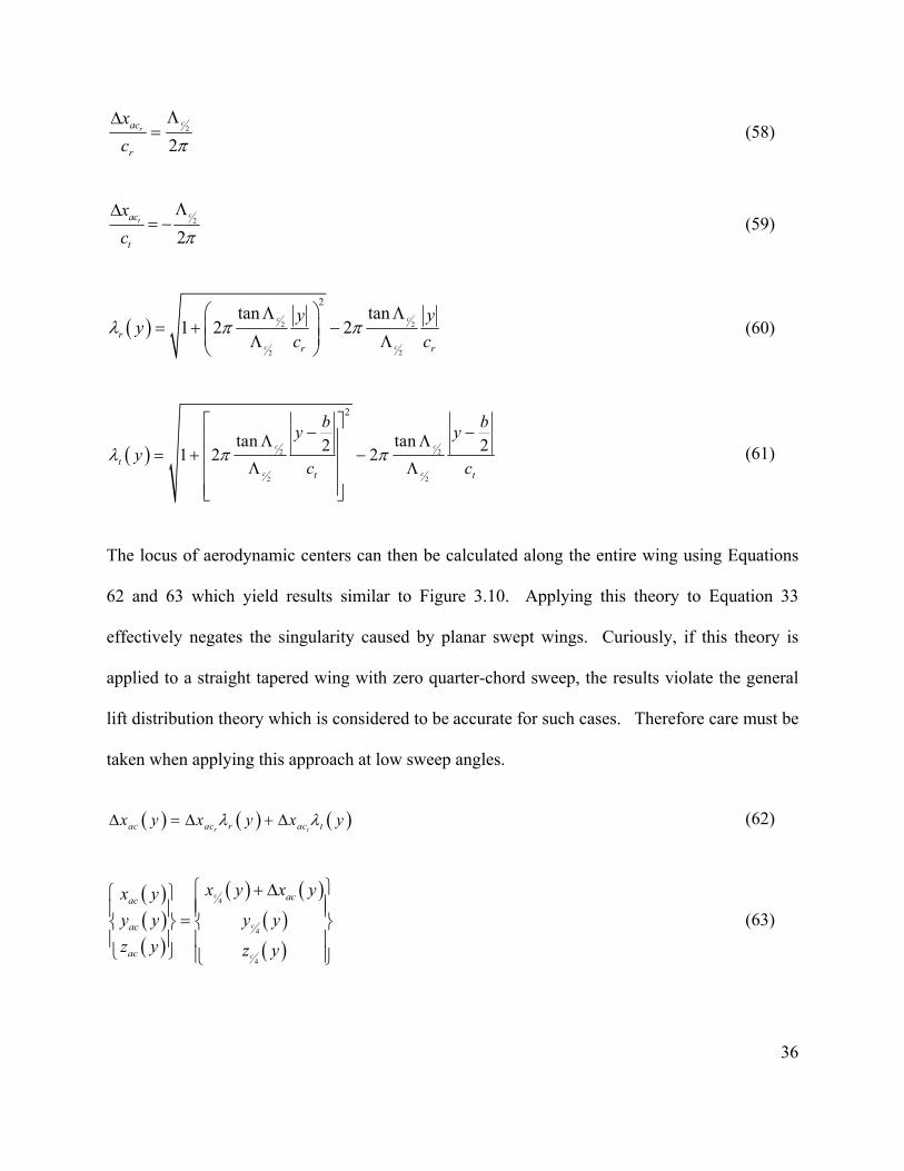
increasing to a maximum of 25% chord at 90˚ sweep as given by Equation 5830. Furthermore,
the aerodynamic center shift at the wing tip is governed by a similar relationship shown in 5930.
Away from the root and tip, the aerodynamic center approaches the quarter chord line
hyperbolically as governed by Equations 6030 and 6130.
36
2
2
crac
r
x
c
(58)
2
2
ctac
t
x
c
(59)
2 2
2 2
2tan tan
1 2 2c c
c c
rr r
y yy
c c
(60)
2 2
2 2
2
tan tan2 21 2 2c c
c c
tt t
b by y
yc c
(61)
The locus of aerodynamic centers can then be calculated along the entire wing using Equations
62 and 63 which yield results similar to Figure 3.10. Applying this theory to Equation 33
effectively negates the singularity caused by planar swept wings. Curiously, if this theory is
applied to a straight tapered wing with zero quarter-chord sweep, the results violate the general
lift distribution theory which is considered to be accurate for such cases. Therefore care must be
taken when applying this approach at low sweep angles.
r tac ac r ac tx y x y x y (62)
4
4
4
c
c
c
acac
ac
ac
x y x yx y
y y y y
z y z y
(63)

37
Figure 3.10 Küchemann A.C. Shift Parameters
Extension to the general cranked case is possible by assuming that the numerical singularities
induced by sweep angle are similar to those caused by dihedral angle and as such can be
accounted for in a similar way. This assumption is seen to be valid by examining the results of
Equation 33 for wings with sweep and dihedral separately without correcting for aerodynamic
center shift. Furthermore, it is assumed that the aerodynamic center shift at any panel root or tip
is caused by the total change in sweep or dihedral angle rather than the magnitude of the sweep
or dihedral angle of that panel, unless at the free tips of the lifting surface.
To avoid the anomaly associated with unswept tapered wings inherent to Küchemann’s
formulation, the quarter-chord angles are used rather than the half-chord angles which cause the
theory to fail. This does cause a slight difference in the results, particularly for panels with low
aspect ratio. However, this difference is seen to have a negligible effect on the results. Figure
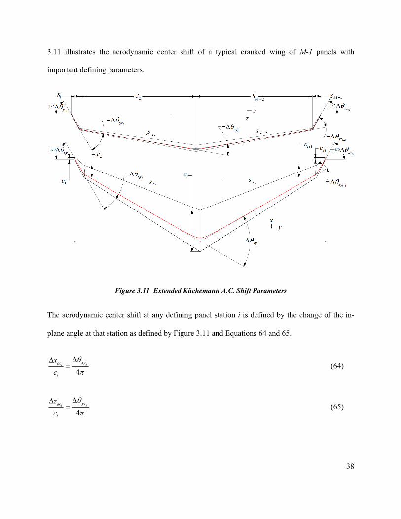
38
3.11 illustrates the aerodynamic center shift of a typical cranked wing of M-1 panels with
important defining parameters.
Figure 3.11 Extended Küchemann A.C. Shift Parameters
The aerodynamic center shift at any defining panel station i is defined by the change of the in-
plane angle at that station as defined by Figure 3.11 and Equations 64 and 65.
4ji
xyac
i
x
c
(64)
4ji
yzac
i
z
c
(65)
39
The hyperbolic blending functions take a similar form to Equations 60 and 61, replacing the y-
coordinate for the span coordinate s as defined by Figure 3.11.
2
1i i i
i ix x x
i i
s s s ss P P
c c
(66)
2
1i i i
i iz z z
i i
s s s ss P P
c c
(67)
Where;
4tan
2i
i
i
xyx
xy
P
(68)
4tan
2i
i
i
yzz
yz
P
(69)
This leads to the aerodynamic center shift and locus functions as follows:
1
i i
M
ac xy xi
x s s
(70)
1
i i
M
ac yz zi
z s s
(71)
4
4
4
c
c
c
acac
ac
ac ac
x s x sx s
y s y s
z s z s z s
(72)
40
3.5 Forces,MomentsandCoefficients
The ultimate goal of coupling the theories documented in the preceding sections is to calculate
the aerodynamic properties of lifting surfaces. As such, the results of the lifting line theory do
not offer much insight on their own. Further post-processing is needed to obtain the forces,
moments and coefficients which characterize the aerodynamics of the lifting surface. Combining
Equations 30 and 32 yields expressions for the force and moment on any differential spanwise
segment as given by Phillips27 via Equations 73 and 74, yet these equations only provide a partial
answer.
1i
Ni j
l i ji ij j
f U vc
(73)
i i i il cg l m i i ai nim r f q c c A u u
(74)
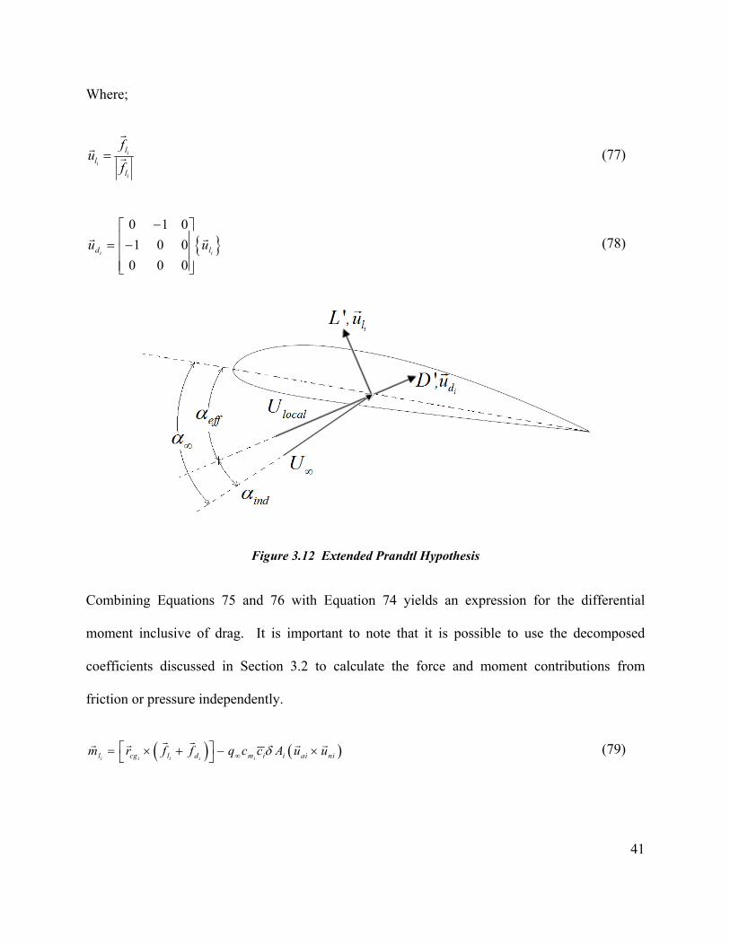
To get a complete picture we must also include drag. By extending Prandtl’s hypothesis that the
sectional lift on a 3D wing acts perpendicular to the local velocity vector to also include the
assumption that drag acts parallel to the velocity vector, we can estimate the drag of the wing
using a similar approach. Figure 3.12 illustrates the extended Prandtl hypothesis. This allows for
the drag on a spanwise differential element to be calculated using Equation 75. Equation 76
offers a similar formulation for lift which is equivalent to Equation 73.
i i id d i df q c Au
(75)
i i il l i lf q c Au
(76)
41
Where;
i
i
i
ll
l
fu
f
(77)
0 1 0
1 0 0
0 0 0i id lu u
(78)
Figure 3.12 Extended Prandtl Hypothesis
Combining Equations 75 and 76 with Equation 74 yields an expression for the differential
moment inclusive of drag. It is important to note that it is possible to use the decomposed
coefficients discussed in Section 3.2 to calculate the force and moment contributions from
friction or pressure independently.
i i i i il cg l d m i i ai nim r f f q c c A u u
(79)
42
The total forces and moments are found by summing the differential contributions of each
spanwise segment as governed by Equations 75, 76 and 79. This takes the form of Equations 80
and 81.
1 1 1
i i i i
N N N
L D l d l di i i
F F F f f f f
(80)
1
i i
N
L D l di
M M M m m
(81)
The aerodynamic force and moment coefficients are in turn calculated using Equations 82 and
83.
cos 0 sin
0 0 0
sin 0 cos
D
Y
L
CF
Cq S
C
(82)
l
mMAC
n
CM
Cq Sc
C
(83)
Where;
/2
/21
cosNb
i ibi
S cdy A
(84)
2
2 1/2 2 1
/2
1
1
cos
i i
N
ibi
MAC Nb
i ii
c y yc c dy
S A
(85)
43
The induced drag can be estimated by considering only lift forces LF
in Equation 82. Ignoring
lift and side-force this becomes Equation 86.
cos sinx zL L
D i
F FC
q S
(86)
4. Application
This section summarizes the application and practical aspects of the theory outlined in Section 0.
Special considerations relating to the computational approach are discussed followed by a
discussion of post-processing and visualization techniques. This is concluded with a brief
overview of a MATLAB code implementing the methods discussed.
4.1 ComputationalConsiderations
There are several special considerations which must be made when applying the theories and
methods outlined in the Section 3. First and foremost is the flexibility of the model, particularly
the lifting line theory. While it can be applied to systems of interacting lifting surfaces with
arbitrary and dynamically varying shapes, finding an algorithm or set of algorithms to explain all
possibilities is virtually impossible. However, by applying the cranked wing model most shapes
and nearly all practical planforms can be approximated if not defined explicitly. Figure 4.1
defines the basic parameters of a cranked wing. Each panel end point is defined by a quarter
chord location, an airfoil section, incidence angle and a chord length. Each panel also has a
characteristic sweep and dihedral angle which is assumed constant at each point in that panel.
Airfoil properties and incidence angle are assumed to vary linearly along the panel. The
44
distribution of points along the panel is of critical importance and Phillips27 suggests that a
cosine distribution will yield the smallest numerical error.
1 cos
2s
(87)
The left and right nodes of the bound vortex segments as well as each control point location are
then assigned a linear location in -space as specified by Equations 88 through 90.
1 0, , ... ,i
pan panN N
(88)
2
2, ... ,
i
pan panN N
(89)
3, ... ,
2 2 2jpan pan panN N N
(90)
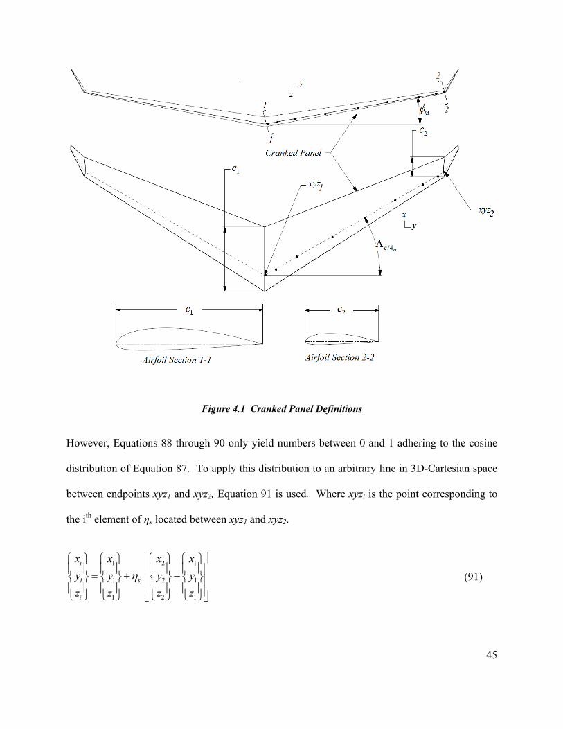
45
Figure 4.1 Cranked Panel Definitions
However, Equations 88 through 90 only yield numbers between 0 and 1 adhering to the cosine
distribution of Equation 87. To apply this distribution to an arbitrary line in 3D-Cartesian space
between endpoints xyz1 and xyz2, Equation 91 is used. Where xyzi is the point corresponding to
the ith element of ηs located between xyz1 and xyz2.
1 2 1
1 2 1
1 2 1
i
i
i s
i
x x x x
y y y y
z z z z
(91)
46
Similarly, relationships which allow for the interpolation of airfoil geometry, lift, drag and
pitching moment, as well as pressure and skin friction distributions to any interior point, can be
established using Equations 87 and 90. These all take a form similar to Equation 91, but
substitute the xyz locations for the appropriate parameters. For example, the section lift
coefficient at any point along the cranked panel can be calculated using the lift coefficients of the
cranked panel end points at the local angle of attack as shown by Equation 92. If interpolating
pressure or skin friction distributions along the panel it is necessary that the values at the panel
endpoints come from identical x/c locations and be from the same surface (i.e. upper vs. lower)
and takes the form of Equation 93.
1 2 1i il i l i s l i l ic c c c (92)
1 2 1
, , , , , , , ,i i
x x x xc c c cp i p i s p i p ic c c c (93)
Another area of importance regarding the calculation is the convergence of Equation 33. This
typically requires that new estimates for G are highly under relaxed. Recommended values for
the relaxation factor Ω of Equation 50 range between 0.7 and 0.9 in most cases and convergence
tolerances of 0.001 to 0.0001 are easily met.
4.2 PostProcessingandVisualization
The forces, moments and coefficients calculated with the equations in Section 3.5 can be used
and understood in a variety of ways. An exhaustive discussion of what is possible is not feasible.
However, some basic aerodynamic properties of interest can be extracted and used at various
phases in the design process, particularly preliminary design. The most basic aerodynamic
47
properties of any lifting surface are its linearized values, such as lift curve slope, zero lift angle
of attack and so on. These values are calculated from the coefficients which result from applying
the proposed methods to a range of angles of attack within the linear range. Assuming
coefficients are known at -6, -3, 0, 3 and 6 degrees angle of attack, the lift curve and lift at zero
angle of attack can be found by applying a 1st order polynomial fit via the least-squares method
which takes the form of Equation 94. From these results, the zero-lift angle of attack is found
using Equation 95.
0L L LC C C (94)
0
0w
L
L
C
C
(95)
The Class-I drag polar can be found in a similar fashion by applying the least-squares method to
an equation of the form dictated by Equation 96. The coefficients of this regression yield zero-
lift drag coefficient and the span efficiency factor via Equations 97 and 98.
20 1D LC A A C (96)
0 0DC A (97)
1
1e
A AR (98)
The linearized pitching moment curve is found in the same manner as the linearized lift curve by
applying a 1st order polynomial fit via the least-squares method. This takes the form of Equation
99 and in turn the zero-lift pitching moment is found via Equation 100.

48
0m m mC C C (99)
00o wm m mC C C (100)
Similarly, the Class-II drag polar is found by applying the least-squares method to a 5th order
polynomial of the form given by Equation 99 to a set of aerodynamic coefficients ranging from -
10 to +10 degrees angle of attack.
0
2 3 4 51 2 3 4 5D L D CD L CD L CD L CD L CD LC C C B C B C B C B C B C (101)
Visualization of the distributed loads is easily accomplished using commercial plotting software
packages such as Tecplot51. By applying a quad-mesh to the lifting surface and using the
methods discussed in Section 4.1, the pressure and skin friction at any point on the surface can
be determined. This in turn allows for the local forces to be calculated using the surface panel
area along with the normal and tangent unit vectors. To create the quad-mesh, the airfoil
coordinates at each station along the cranked panel are interpolated using Equation 102 then
scaled using the local chord.
1 2 1, , , ,i
i x x x xc c c cs
z z z z
c c c c
(102)
Following interpolation and scaling of the airfoil coordinates, they are rotated to the proper
incidence and dihedral angle via Equation 103 and then transformed to the quarter-chord location
via Equation 104.
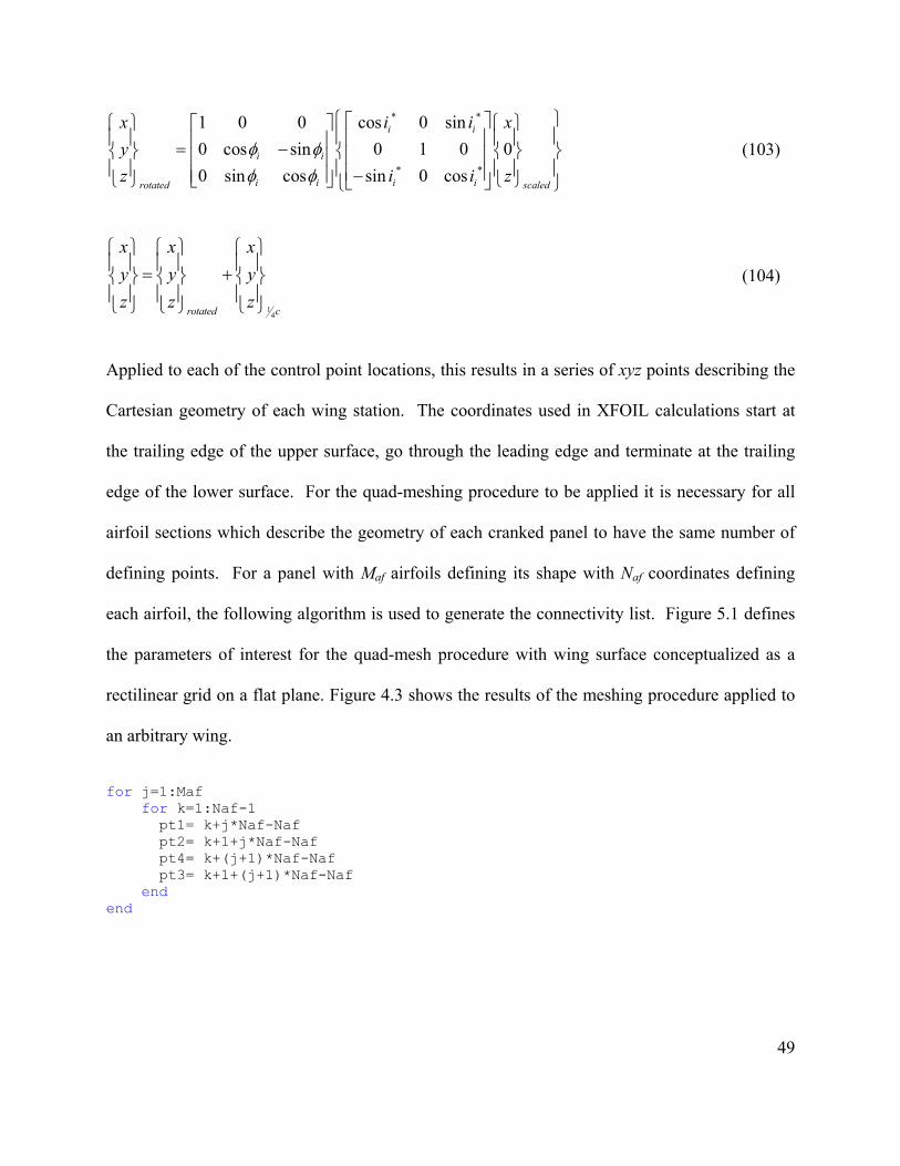
49
* *
* *
1 0 0 cos 0 sin
0 cos sin 0 1 0 0
0 sin cos sin 0 cos
i i
i i
i i i irotated scaled
x i i x
y
z i i z
(103)
14rotated c
x x x
y y y
z z z
(104)
Applied to each of the control point locations, this results in a series of xyz points describing the
Cartesian geometry of each wing station. The coordinates used in XFOIL calculations start at
the trailing edge of the upper surface, go through the leading edge and terminate at the trailing
edge of the lower surface. For the quad-meshing procedure to be applied it is necessary for all
airfoil sections which describe the geometry of each cranked panel to have the same number of
defining points. For a panel with Maf airfoils defining its shape with Naf coordinates defining
each airfoil, the following algorithm is used to generate the connectivity list. Figure 5.1 defines
the parameters of interest for the quad-mesh procedure with wing surface conceptualized as a
rectilinear grid on a flat plane. Figure 4.3 shows the results of the meshing procedure applied to
an arbitrary wing.
for j=1:Maf for k=1:Naf-1 pt1= k+j*Naf-Naf pt2= k+1+j*Naf-Naf pt4= k+(j+1)*Naf-Naf pt3= k+1+(j+1)*Naf-Naf end end

50
Figure 4.2 Quad-Mesh Parameters
Figure 4.3 Example of Meshing Procedure Results
This results in af afN M points at which the pressure and skin friction are calculated using the
method outlined in Section 4.1. For each of the 1af afN M quad elements defined by points
1-4, the panel normal and tangential unit vectors are found via Equations 105 and 106 while the
surface panel area is found via Equation 107.
1ˆ
2n a b c d (105)

51
0 1 0
ˆ ˆ1 0 0
0 0 0
t n
(106)
sA a b (107)
Where;
2 1
2 1
2 1
x x
a y y
z z
(108)
4 1
4 1
4 1
x x
b y y
z z
(109)
3 2
3 2
3 2
x x
c y y
z z
(110)
3 4
3 4
3 4
x x
d y y
z z
(111)
This allows for the pressure and skin friction to be decomposed into fx, fy, fz or fx/As, fy/As, fz /As at
each of the points on the surface yielding data useful for FEA analysis via Equation 112.
52
ˆˆx
y s
z
f
f p n t A
f
(112)
4.3 AdvancedPlanformAnalysisandXFOILultra
The methods outlined in Sections 3.1 through 4.2 have been implemented into a pair of
MATLAB6 codes called Advanced Planform Analysis and XFOILultra (see Appendix A) with
each containing several subroutines. XFOILultra operates XFOIL17 in batch mode by
constructing a text based input file, executing the file and importing the results to MATLAB.
This is done for angles of attack ranging from -10 to +20 degrees followed by extrapolation
using the Viterna method. This yields a complete breakdown of aerodynamic coefficients and
pressure and friction distributions which are then passed to Advanced Planform Analysis.
Geometry, operating condition, calculation settings and post processing options for Advanced
Planform Analysis are contained within a spreadsheet. All geometry definitions assume the
cranked wing method and results are displayed in both textual and graphical format. Surface
plots are created by generating Tecplot input files which conform to the quad-meshing procedure
already discussed.
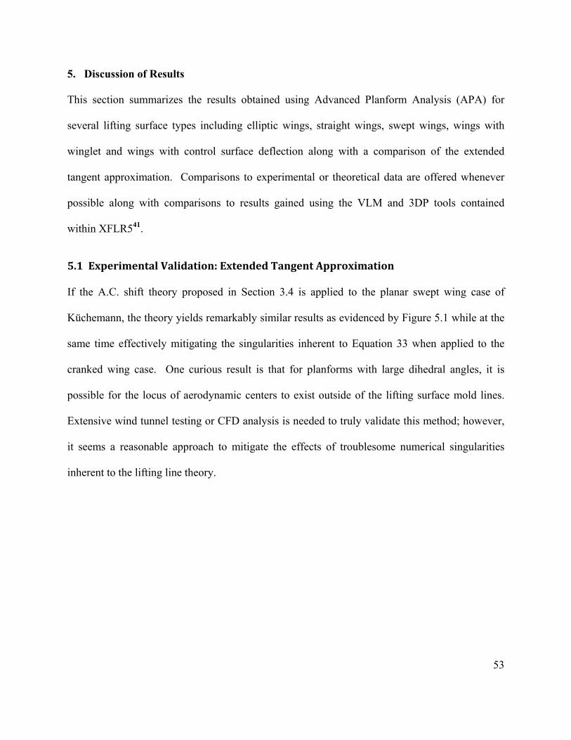
53
5. Discussion of Results
This section summarizes the results obtained using Advanced Planform Analysis (APA) for
several lifting surface types including elliptic wings, straight wings, swept wings, wings with
winglet and wings with control surface deflection along with a comparison of the extended
tangent approximation. Comparisons to experimental or theoretical data are offered whenever
possible along with comparisons to results gained using the VLM and 3DP tools contained
within XFLR541.
5.1 ExperimentalValidation:ExtendedTangentApproximation
If the A.C. shift theory proposed in Section 3.4 is applied to the planar swept wing case of
Küchemann, the theory yields remarkably similar results as evidenced by Figure 5.1 while at the
same time effectively mitigating the singularities inherent to Equation 33 when applied to the
cranked wing case. One curious result is that for planforms with large dihedral angles, it is
possible for the locus of aerodynamic centers to exist outside of the lifting surface mold lines.
Extensive wind tunnel testing or CFD analysis is needed to truly validate this method; however,
it seems a reasonable approach to mitigate the effects of troublesome numerical singularities
inherent to the lifting line theory.

54
Figure 5.1 Comparison of Tangent Approximations to Experimental Data
For the special case of untapered planar wings, the extended tangent approximation reduces to
Küchemann’s tangent approximation exactly. Yet, for wings with taper disagreement arises with
the differences becoming more extreme for wings with large taper or low aspect ratio where the
difference between quarter-chord sweep angle and half-chord sweep angle can be quite
significant. Nevertheless, the extended tangent approximation matches available experimental
data with exceptional accuracy and effectively mitigates the singularity of the lifting line method
for cranked wings.
5.2 TheoreticalValidation:EllipticWing
Prandtl’s classic closed form solution to the elliptic wing problem can be found in many
textbooks and provides a simple and accurate method to check the results of APA. For a straight
wing with an elliptic chord distribution given by Equation 1137, the circulation distribution along
the wing is assumed to also be elliptic and is given by Equation 1147.
2
1 2r
yc y c
b
(113)
0.0 0.1 0.2 0.3 0.4 0.5 0.6 0.7 0.8 0.9 1.0-0.20
-0.15
-0.10
-0.05
0.00
0.05
0.10
0.15
0.20
Span Location, = 2y/b [~]
Aer
ody
nam
ic C
ente
r S
hift
,
x ac/c
r [~]
Kuchemann (Ref. 30) AR=8, =0.50
Proposed Method AR=8, =0.50
Exp. Data (Ref. 49) AR=8, =0.50
Kuchemann (Ref. 30) AR=3, =0.45
Proposed Method AR=3, =0.45
Exp. Data (Ref. 50) AR=3, =0.45

55
2
0 1 2y
yb
(114)
Where;
0 2 L
SU C
b
(115)
The planform lift coefficient is found from Equation 1167 with the planform lift curve slope
dictated by Equation 1177. This assumes that the airfoil section is constant along the wing with
no twist or incidence.
wL L oC C
` (116)
1
lL
l
cC
c
AR
(117)
The induced drag of an elliptic wing is found by applying Equation 1187 to the calculated
planform lift coefficient. An interesting consequence of Prandtl’s solution is that the downwash
along the wing is constant leading to fact that the planform zero-lift angle of attack for the wing
is the same as that of the airfoil section used as illustrated by Equation 119.
2
i
LD
CC
AR (118)
0 0w (119)

56
A comparison of the predicted results to Prandtl’s solution reveals that APA handles the elliptic
wing problem with exceptional accuracy. The predicted circulation distributions on elliptic
wings agree almost exactly with Equation 114. Figure 5.2 shows the predicted circulation
distribution on elliptic wings of varying aspect ratio with NACA 2312 airfoil section at 5 degrees
angle of attack and Reynolds number of 2.4e6.
Figure 5.2 Predicted and Theoretical Circulation on Elliptic Wings, α=5˚, Re=2.4e6
The small amount of disagreement between Equation 114 and APA can be attributed to the slight
mismatch in lift coefficient when calculated using linearized properties and when found or
interpolated from a look up table as is the case with APA.
The predicted lift curve slope and induced drag polar are also seen to agree almost exactly with
Equations 116 and 118. Figure 5.3 and Figure 5.4 show a comparison of induced drag polars and
lift curve slope for elliptic wings of varying aspect ratio with NACA 2312 airfoil section at a
Reynolds number of 2.4e6.
-1.0 -0.8 -0.6 -0.4 -0.2 0.0 0.2 0.4 0.6 0.8 1.00
20
40
60
80
100
120
Span Location, =2y/b [~]
Circ
ula
tion
, [f
t2 /s]
Eq. 114, AR=4 APA, AR=4 Eq. 114, AR=8 APA, AR=8 Eq. 114, AR=12 APA, AR=12 Eq. 114, AR=16 APA, AR=16
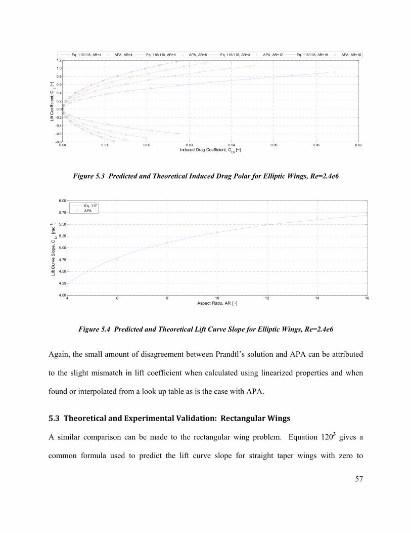
57
Figure 5.3 Predicted and Theoretical Induced Drag Polar for Elliptic Wings, Re=2.4e6
Figure 5.4 Predicted and Theoretical Lift Curve Slope for Elliptic Wings, Re=2.4e6
Again, the small amount of disagreement between Prandtl’s solution and APA can be attributed
to the slight mismatch in lift coefficient when calculated using linearized properties and when
found or interpolated from a look up table as is the case with APA.
5.3 TheoreticalandExperimentalValidation:RectangularWings
A similar comparison can be made to the rectangular wing problem. Equation 1203 gives a
common formula used to predict the lift curve slope for straight taper wings with zero to
0.00 0.01 0.02 0.03 0.04 0.05 0.06 0.07-0.8
-0.6
-0.4
-0.2
0.0
0.2
0.4
0.6
0.8
1.0
1.2
Induced Drag Coefficient, CDi
[~]
Lift
Coe
ffici
ent
, CL [~
]
Eq. 116/118, AR=4 APA, AR=4 Eq. 116/118, AR=8 APA, AR=8 Eq. 116/118, AR=4 APA, AR=12 Eq. 116/118, AR=16 APA, AR=16
4 6 8 10 12 14 164.00
4.25
4.50
4.75
5.00
5.25
5.50
5.75
6.00
Aspect Ratio, AR [~]
Lift
Cur
ve S
lop
e, C
L [r
ad-1
]
Eq. 117APA
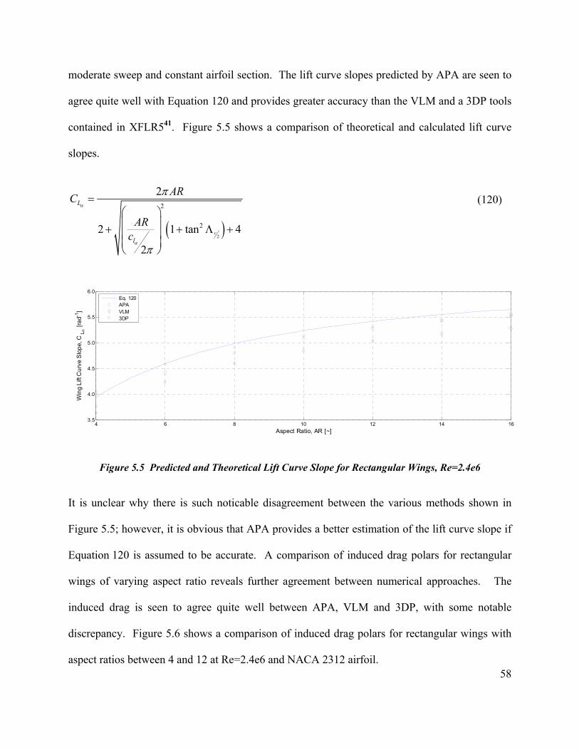
58
moderate sweep and constant airfoil section. The lift curve slopes predicted by APA are seen to
agree quite well with Equation 120 and provides greater accuracy than the VLM and a 3DP tools
contained in XFLR541. Figure 5.5 shows a comparison of theoretical and calculated lift curve
slopes.
2
2
2
2
2 1 tan 4
2
c
L
l
ARC
ARc
(120)
Figure 5.5 Predicted and Theoretical Lift Curve Slope for Rectangular Wings, Re=2.4e6
It is unclear why there is such noticable disagreement between the various methods shown in
Figure 5.5; however, it is obvious that APA provides a better estimation of the lift curve slope if
Equation 120 is assumed to be accurate. A comparison of induced drag polars for rectangular
wings of varying aspect ratio reveals further agreement between numerical approaches. The
induced drag is seen to agree quite well between APA, VLM and 3DP, with some notable
discrepancy. Figure 5.6 shows a comparison of induced drag polars for rectangular wings with
aspect ratios between 4 and 12 at Re=2.4e6 and NACA 2312 airfoil.
4 6 8 10 12 14 163.5
4.0
4.5
5.0
5.5
6.0
Aspect Ratio, AR [~]
Win
g L
ift C
urv
e S
lop
e, C
L [r
ad-1
]
Eq. 120APAVLM3DP
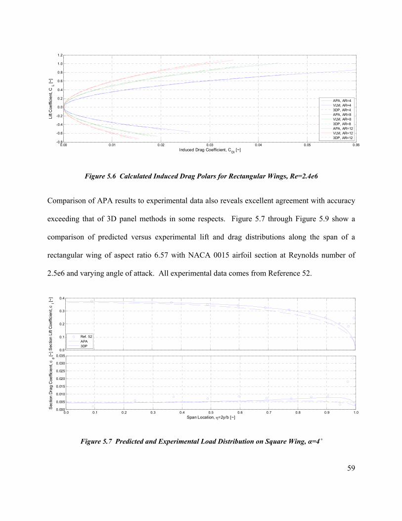
59
Figure 5.6 Calculated Induced Drag Polars for Rectangular Wings, Re=2.4e6
Comparison of APA results to experimental data also reveals excellent agreement with accuracy
exceeding that of 3D panel methods in some respects. Figure 5.7 through Figure 5.9 show a
comparison of predicted versus experimental lift and drag distributions along the span of a
rectangular wing of aspect ratio 6.57 with NACA 0015 airfoil section at Reynolds number of
2.5e6 and varying angle of attack. All experimental data comes from Reference 52.
Figure 5.7 Predicted and Experimental Load Distribution on Square Wing, α=4˚
0.00 0.01 0.02 0.03 0.04 0.05 0.06-0.8
-0.6
-0.4
-0.2
0.0
0.2
0.4
0.6
0.8
1.0
1.2
Induced Drag Coefficient, CDi
[~]
Lift
Coe
ffici
ent
, CL [~
]
APA, AR=4VLM, AR=43DP, AR=4APA, AR=8VLM, AR=83DP, AR=8APA, AR=12VLM, AR=123DP, AR=12
0.0
0.1
0.2
0.3
0.4
Sec
tion
Lift
Co
effic
ien
t, c
l [~]
Ref. 52APA3DP
0.0 0.1 0.2 0.3 0.4 0.5 0.6 0.7 0.8 0.9 1.00.000
0.005
0.010
0.015
0.020
0.025
0.030
0.035
Span Location, =2y/b [~]
Sec
tion
Dra
g C
oeffi
cie
nt, c
d [~]
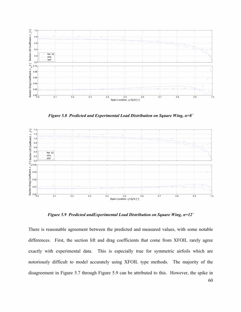
60
Figure 5.8 Predicted and Experimental Load Distribution on Square Wing, α=8˚
Figure 5.9 Predicted andExperimental Load Distribution on Square Wing, α=12˚
There is reasonable agreement between the predicted and measured values, with some notable
differences. First, the section lift and drag coefficients that come from XFOIL rarely agree
exactly with experimental data. This is especially true for symmetric airfoils which are
notoriously difficult to model accurately using XFOIL type methods. The majority of the
disagreement in Figure 5.7 through Figure 5.9 can be attributed to this. However, the spike in
0.0
0.2
0.4
0.6
0.8
1.0S
ectio
n L
ift C
oef
ficie
nt,
cl [~
]
Ref. 52APA3DP
0.0 0.1 0.2 0.3 0.4 0.5 0.6 0.7 0.8 0.9 1.00.00
0.02
0.04
0.06
0.08
0.10
Span Location, =2y/b [~]
Sec
tion
Dra
g C
oeffi
cie
nt, c
d [~]
0.0
0.2
0.4
0.6
0.8
1.0
1.2
1.4
Sec
tion
Lift
Co
effic
ien
t, c
l [~]
Ref. 52APA3DP
0.0 0.1 0.2 0.3 0.4 0.5 0.6 0.7 0.8 0.9 1.00.00
0.01
0.02
0.03
0.04
Span Location, =2y/b [~]
Sec
tion
Dra
g C
oeffi
cie
nt, c
d [~]
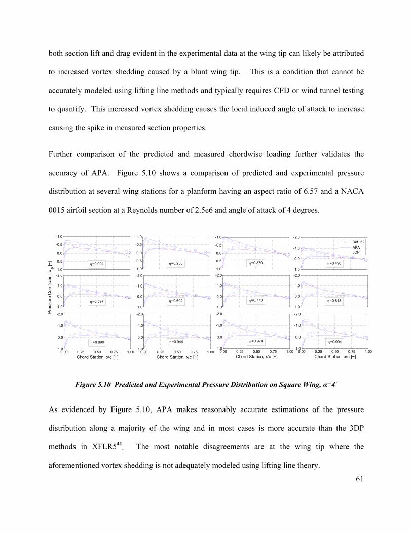
61
both section lift and drag evident in the experimental data at the wing tip can likely be attributed
to increased vortex shedding caused by a blunt wing tip. This is a condition that cannot be
accurately modeled using lifting line methods and typically requires CFD or wind tunnel testing
to quantify. This increased vortex shedding causes the local induced angle of attack to increase
causing the spike in measured section properties.
Further comparison of the predicted and measured chordwise loading further validates the
accuracy of APA. Figure 5.10 shows a comparison of predicted and experimental pressure
distribution at several wing stations for a planform having an aspect ratio of 6.57 and a NACA
0015 airfoil section at a Reynolds number of 2.5e6 and angle of attack of 4 degrees.
Figure 5.10 Predicted and Experimental Pressure Distribution on Square Wing, α=4˚
As evidenced by Figure 5.10, APA makes reasonably accurate estimations of the pressure
distribution along a majority of the wing and in most cases is more accurate than the 3DP
methods in XFLR541. The most notable disagreements are at the wing tip where the
aforementioned vortex shedding is not adequately modeled using lifting line theory.
-1.0
-0.5
0.0
0.5
1.0
-1.0
-0.5
0.0
0.5
1.0
-1.0
-0.5
0.0
0.5
1.0
-2.0
-1.0
0.0
1.0
-2.0
-1.0
0.0
1.0
-2.0
-1.0
0.0
1.0
-2.0
-1.0
0.0
1.0
-2.0
-1.0
0.0
1.0
0.00 0.25 0.50 0.75 1.00
-2.0
-1.0
0.0
1.0
Chord Station, x/c [~]0.00 0.25 0.50 0.75 1.00
-2.0
-1.0
0.0
1.0
Chord Station, x/c [~]0.00 0.25 0.50 0.75 1.00
-2.0
-1.0
0.0
1.0
Chord Station, x/c [~]0.00 0.25 0.50 0.75 1.00
-2.0
-1.0
0.0
1.0
Chord Station, x/c [~]
Pre
ssu
re C
oeffi
cie
nt, c
p [~]
Ref. 52APA3DP
=0.094 =0.238 =0.370 =0.490
=0.597 =0.692 =0.773 =0.843
=0.899 =0.944 =0.974 =0.994
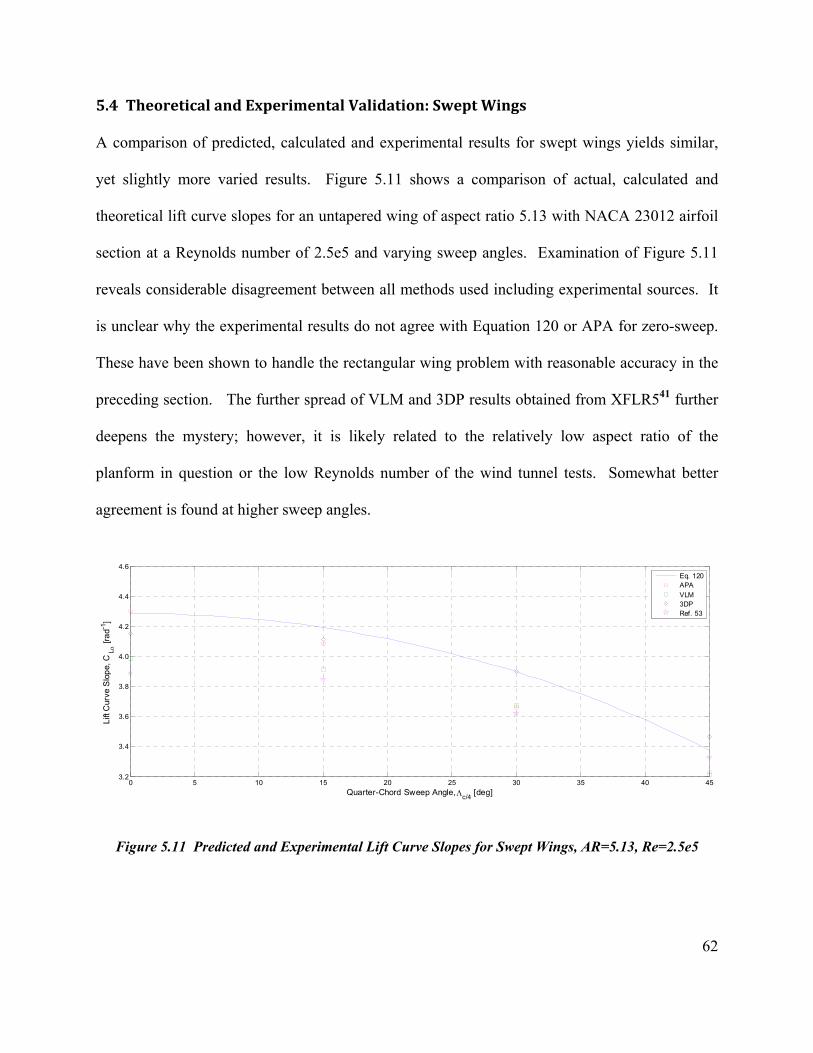
62
5.4 TheoreticalandExperimentalValidation:SweptWings
A comparison of predicted, calculated and experimental results for swept wings yields similar,
yet slightly more varied results. Figure 5.11 shows a comparison of actual, calculated and
theoretical lift curve slopes for an untapered wing of aspect ratio 5.13 with NACA 23012 airfoil
section at a Reynolds number of 2.5e5 and varying sweep angles. Examination of Figure 5.11
reveals considerable disagreement between all methods used including experimental sources. It
is unclear why the experimental results do not agree with Equation 120 or APA for zero-sweep.
These have been shown to handle the rectangular wing problem with reasonable accuracy in the
preceding section. The further spread of VLM and 3DP results obtained from XFLR541 further
deepens the mystery; however, it is likely related to the relatively low aspect ratio of the
planform in question or the low Reynolds number of the wind tunnel tests. Somewhat better
agreement is found at higher sweep angles.
Figure 5.11 Predicted and Experimental Lift Curve Slopes for Swept Wings, AR=5.13, Re=2.5e5
0 5 10 15 20 25 30 35 40 453.2
3.4
3.6
3.8
4.0
4.2
4.4
4.6
Quarter-Chord Sweep Angle, c/4 [deg]
Lift
Cur
ve S
lop
e, C
L [r
ad-1
]
Eq. 120APAVLM3DPRef. 53
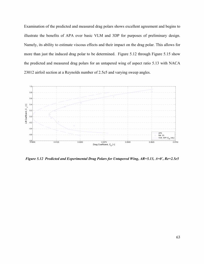
63
Examination of the predicted and measured drag polars shows excellent agreement and begins to
illustrate the benefits of APA over basic VLM and 3DP for purposes of preliminary design.
Namely, its ability to estimate viscous effects and their impact on the drag polar. This allows for
more than just the induced drag polar to be determined. Figure 5.12 through Figure 5.15 show
the predicted and measured drag polars for an untapered wing of aspect ratio 5.13 with NACA
23012 airfoil section at a Reynolds number of 2.5e5 and varying sweep angles.
Figure 5.12 Predicted and Experimental Drag Polars for Untapered Wing, AR=5.13, Λ=0˚, Re=2.5e5
0.0000 0.0125 0.0250 0.0375 0.0500 0.0625 0.0750-0.8
-0.6
-0.4
-0.2
0.0
0.2
0.4
0.6
0.8
1.0
Drag Coefficient, CD
[~]
Lift
Coe
ffici
ent
, CL [~
]
APARef. 53VLM, 3DP (C
Di only)

64
Figure 5.13 Predicted and Experimental Drag Polars for Untapered Wing, AR=5.13, Λ=15˚, Re=2.5e5
Figure 5.14 Predicted and Experimental Drag Polars for Untapered Wing, AR=5.13, Λ=30˚, Re=2.5e5
0.0000 0.0125 0.0250 0.0375 0.0500 0.0625 0.0750-0.8
-0.6
-0.4
-0.2
0.0
0.2
0.4
0.6
0.8
1.0
Drag Coefficient, CD
[~]
Lift
Coe
ffici
ent
, CL [~
]
APARef. 53VLM,3DP (CDi only)
0.0000 0.0125 0.0250 0.0375 0.0500 0.0625 0.0750-0.8
-0.6
-0.4
-0.2
0.0
0.2
0.4
0.6
0.8
Drag Coefficient, CD
[~]
Lift
Coe
ffici
ent
, CL [~
]
APARef. 53VLM, 3DP (C
Di only)

65
Figure 5.15 Predicted and Experimental Drag Polars for Untapered Wing, AR=5.13, Λ=45˚, Re=2.5e5
The agreement of the drag polars predicted by APA and those from Reference 53 is reasonable
evidence that methods employed for estimating the viscous drag distribution in APA are accurate
enough for preliminary design purposes. The zero-lift drag and drag polar trends are adequately
modeled with decreasing accuracy at higher angles of attack. Nevertheless, it provides a better
total estimation of the wing aerodynamics than the VLM and 3DP methods used.
Despite relative agreement of the lift curve slope and drag polars, the predicted spanwise loading
seems to not match as well as it did for straight wings. Figure 5.16 shows the normal force
distribution on an untapered wing of aspect ratio 5.13 with NACA 23012 airfoil section at a
Reynolds number of 2.5e5 and angle of attack of 8.5 degrees and varying sweep angles.
0.0000 0.0125 0.0250 0.0375 0.0500 0.0625 0.0750-0.8
-0.6
-0.4
-0.2
0.0
0.2
0.4
0.6
Drag Coefficient, CD
[~]
Lift
Coe
ffici
ent
, CL [~
]
APARef. 53VLM, 3DP (CDi only)

66
Figure 5.16 Predicted and Experimental Normal Force Distribution on Swept Wings, AR=5.13, α=8.5˚
Examination of Figure 5.16 reveals some troubling behavior of the lifting line theory used in
APA. While the tangent approximation mitigates the singularities caused by discontinuities of
the first derivative of the quarter-chord line, it does not adequately predict the downwash near
these discontinuities. This leads to an over estimation in angle of attack and ultimately the
predicted lift. However, APA still offers a fairly accurate approximation of swept wing
aerodynamics with exceptional accuracy in the prediction of drag polars and linear lift
characteristics. The distributed loads are also predicted with reasonable accuracy, appropriate
for the preliminary design phase. Figure 5.17 through Figure 5.20 show the pressure
distributions predicted using the 3DP tool in XFLR5 and APA.
0.0
0.5
1.0
Ref. 53PanelAPA
0.0
0.5
1.0
1.5
Nor
ma
l Fo
rce
Co
effi
cien
t, c
n [~]
0.0
1.0
2.0
0.0 0.1 0.2 0.3 0.4 0.5 0.6 0.7 0.8 0.9 1.00.0
0.5
1.0
1.5
Span Location, = 2y/b [~]
c/4 = 0 deg
c/4 = 15 deg
c/4 = 30 deg
c/4 = 45 deg
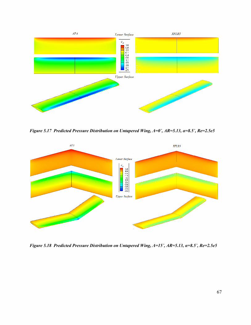
67
Figure 5.17 Predicted Pressure Distribution on Untapered Wing, Λ=0˚, AR=5.13, α=8.5˚, Re=2.5e5
Figure 5.18 Predicted Pressure Distribution on Untapered Wing, Λ=15˚, AR=5.13, α=8.5˚, Re=2.5e5

68
Figure 5.19 Predicted Pressure Distribution on Untapered Wing, Λ=30˚, AR=5.13, α=8.5˚, Re=2.5e5
Figure 5.20 Predicted Pressure Distribution on Untapered Wing, Λ=45˚, AR=5.13, α=8.5˚, Re=2.5e5

69
As expected, there is not perfect agreement between the pressure distributions predicted using
3D panel methods and those obtained from APA. The exaggerated downwash of the lifting line
theory causes noticeable disagreement at the wing root. At large enough sweep angles this can
cause the local angle of attack to push into the post-stall region resulting in the application of the
assumed Viterna distributions. This is evidenced by the solid color strips located at the root of
the wing on the left hand side of Figure 5.20. Nevertheless, the predicted distributions are
reasonable and certainly accurate enough for preliminary design purposes. Especially in light of
the results of Section 5.3 which showed APA to be more accurate than the panel method in
XFLR5 for rectangular wings and the exceptional accuracy of the drag polar predictions for
swept wings discussed earlier in this section.
5.5 ExperimentalValidation:WingwithControlSurfaceDeflection
The analysis of lifting surfaces with control surface deflection is easily handled by the current
method but with varying degrees of accuracy. This is accomplished by using the geometry
modification functions built into XFOIL to alter the airfoil coordinates to approximate the
deflected section geometry. XFOIL then analyzes the airfoil as usual, but this analysis is limited
to plain flaps, ailerons or similar type controls with deflections less than 30 degrees. Figure 5.21
through Figure 5.23 show the lift curves and drag polars for a rectangular wing of aspect ratio
3.13 with NACA 64A010 airfoil section equipped with inboard half-span plain flaps at Reynolds
number of 4.5e6 and deflection angles of 0˚, 10˚ and 20˚.
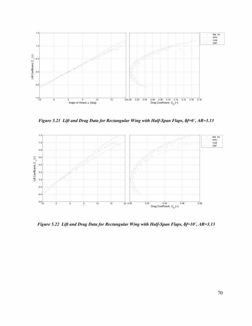
70
Figure 5.21 Lift and Drag Data for Rectangular Wing with Half-Span Flaps, δf=0˚, AR=3.13
Figure 5.22 Lift and Drag Data for Rectangular Wing with Half-Span Flaps, δf=10˚, AR=3.13
-10 -5 0 5 10 15 20-1.0
-0.5
0.0
0.5
1.0
1.5
Angle of Attack, [deg]
Lift
Coe
ffici
ent
, CL [~
]
0.00 0.02 0.04 0.06 0.08 0.10 0.12 0.14 0.16 0.18
Drag Coefficient, CD
[~]
Ref. 54APAVLM3DP
-10 -5 0 5 10 15 20-0.6
-0.4
-0.2
0.0
0.2
0.4
0.6
0.8
1.0
1.2
Angl e of Attac k , [deg]
Lift
Coe
ffici
ent
, CL [~
]
0.00 0.02 0.04 0.06 0.08
Drag Coefficient, CD
[~]
Ref. 54APAVLM3DP
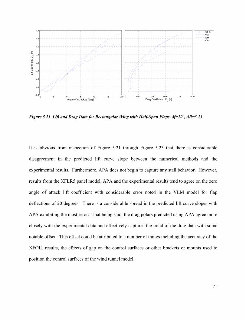
71
Figure 5.23 Lift and Drag Data for Rectangular Wing with Half-Span Flaps, δf=20˚, AR=3.13
It is obvious from inspection of Figure 5.21 through Figure 5.23 that there is considerable
disagreement in the predicted lift curve slope between the numerical methods and the
experimental results. Furthermore, APA does not begin to capture any stall behavior. However,
results from the XFLR5 panel model, APA and the experimental results tend to agree on the zero
angle of attack lift coefficient with considerable error noted in the VLM model for flap
deflections of 20 degrees. There is a considerable spread in the predicted lift curve slopes with
APA exhibiting the most error. That being said, the drag polars predicted using APA agree more
closely with the experimental data and effectively captures the trend of the drag data with some
notable offset. This offset could be attributed to a number of things including the accuracy of the
XFOIL results, the effects of gap on the control surfaces or other brackets or mounts used to
position the control surfaces of the wind tunnel model.
-10 -5 0 5 10 15 20-0.2
0.0
0.2
0.4
0.6
0.8
1.0
1.2
1.4
Angle of Attack, [deg]
Lift
Coe
ffici
ent
, CL [~
]
0.00 0.02 0.04 0.06 0.08 0.10
Drag Coefficient, CD
[~]
Ref. 54APAVLM3DP
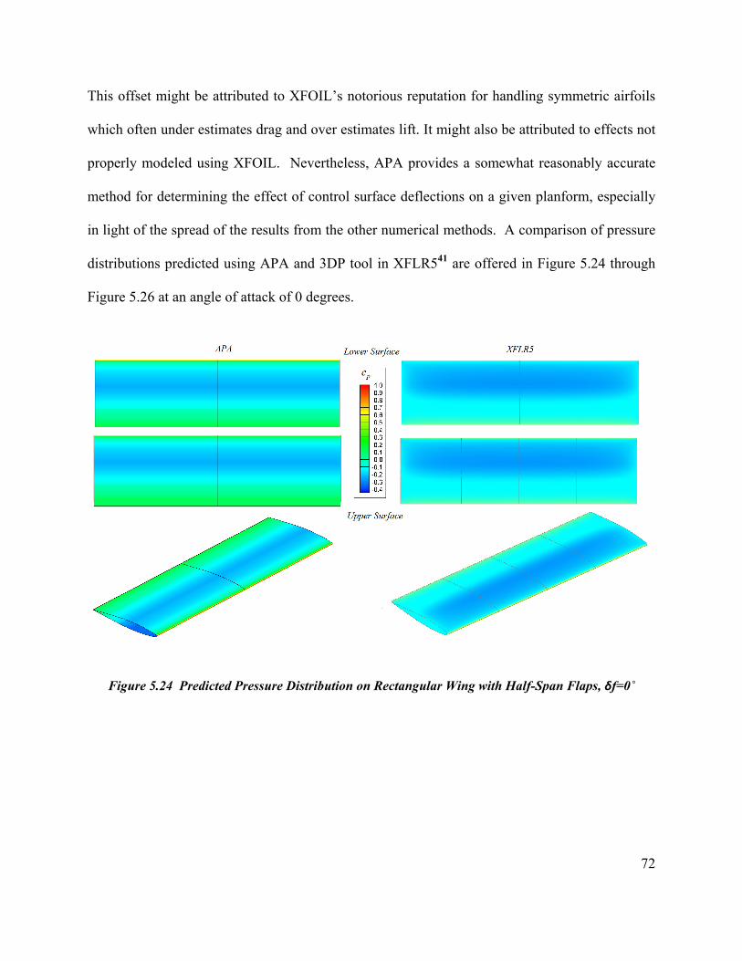
72
This offset might be attributed to XFOIL’s notorious reputation for handling symmetric airfoils
which often under estimates drag and over estimates lift. It might also be attributed to effects not
properly modeled using XFOIL. Nevertheless, APA provides a somewhat reasonably accurate
method for determining the effect of control surface deflections on a given planform, especially
in light of the spread of the results from the other numerical methods. A comparison of pressure
distributions predicted using APA and 3DP tool in XFLR541 are offered in Figure 5.24 through
Figure 5.26 at an angle of attack of 0 degrees.
Figure 5.24 Predicted Pressure Distribution on Rectangular Wing with Half-Span Flaps, δf=0˚

73
Figure 5.25 Predicted Pressure Distribution on Rectangular Wing with Half-Span Flaps, δf=10˚
Figure 5.26 Predicted Pressure Distribution on Rectangular Wing with Half-Span Flaps, δf=20˚
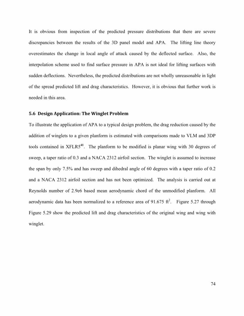
74
It is obvious from inspection of the predicted pressure distributions that there are severe
discrepancies between the results of the 3D panel model and APA. The lifting line theory
overestimates the change in local angle of attack caused by the deflected surface. Also, the
interpolation scheme used to find surface pressure in APA is not ideal for lifting surfaces with
sudden deflections. Nevertheless, the predicted distributions are not wholly unreasonable in light
of the spread predicted lift and drag characteristics. However, it is obvious that further work is
needed in this area.
5.6 DesignApplication:TheWingletProblem
To illustrate the application of APA to a typical design problem, the drag reduction caused by the
addition of winglets to a given planform is estimated with comparisons made to VLM and 3DP
tools contained in XFLR541. The planform to be modified is planar wing with 30 degrees of
sweep, a taper ratio of 0.3 and a NACA 2312 airfoil section. The winglet is assumed to increase
the span by only 7.5% and has sweep and dihedral angle of 60 degrees with a taper ratio of 0.2
and a NACA 2312 airfoil section and has not been optimized. The analysis is carried out at
Reynolds number of 2.9e6 based mean aerodynamic chord of the unmodified planform. All
aerodynamic data has been normalized to a reference area of 91.675 ft2. Figure 5.27 through
Figure 5.29 show the predicted lift and drag characteristics of the original wing and wing with
winglet.
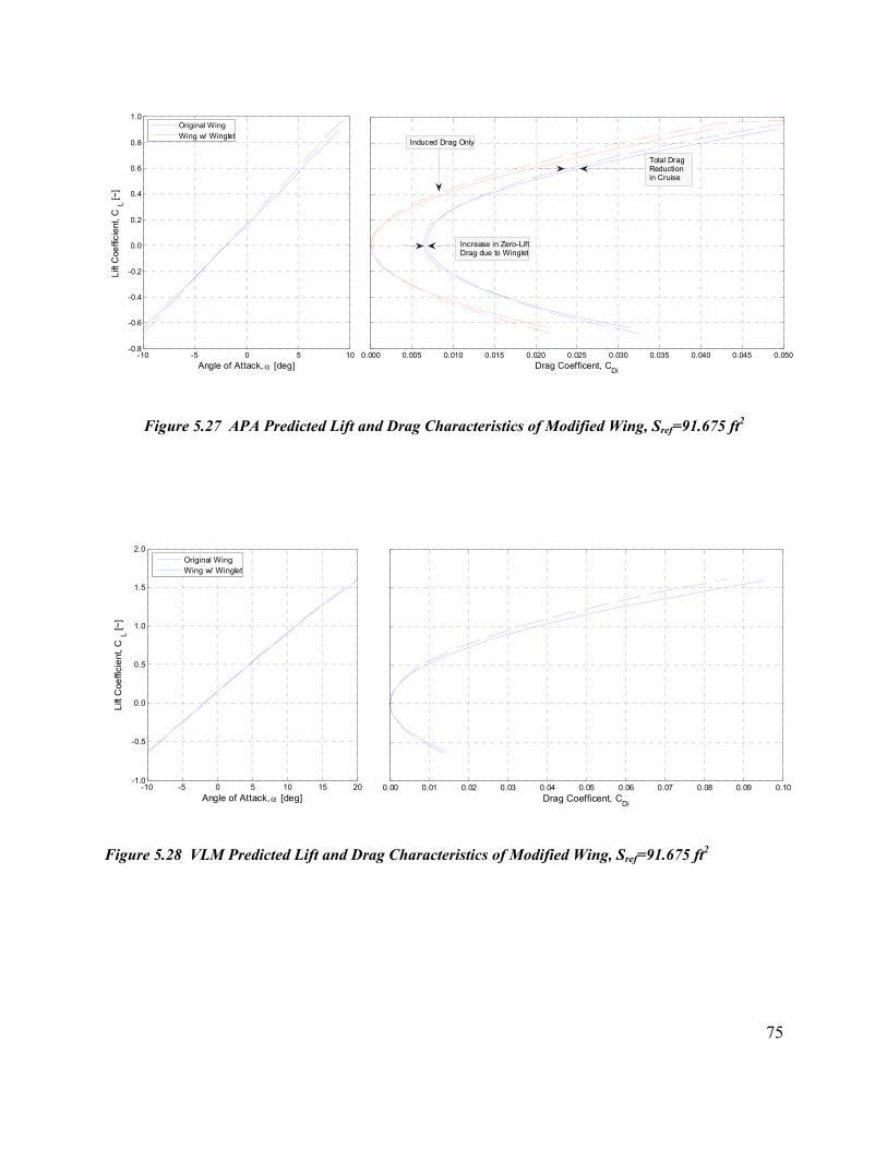
75
Figure 5.27 APA Predicted Lift and Drag Characteristics of Modified Wing, Sref=91.675 ft2
Figure 5.28 VLM Predicted Lift and Drag Characteristics of Modified Wing, Sref=91.675 ft2
-10 -5 0 5 10-0.8
-0.6
-0.4
-0.2
0.0
0.2
0.4
0.6
0.8
1.0
Angle of Attack, [deg]
Lift
Coe
ffici
ent
, CL [~
]
0.000 0.005 0.010 0.015 0.020 0.025 0.030 0.035 0.040 0.045 0.050
Drag Coefficent, CDi
Original WingWing w/ Winglet
Induced Drag Only
Increase in Zero-LiftDrag due to Winglet
Total DragReductionin Cruise
-10 -5 0 5 10 15 20-1.0
-0.5
0.0
0.5
1.0
1.5
2.0
Angle of Attack, [deg]
Lift
Coe
ffici
ent
, CL [~
]
0.00 0.01 0.02 0.03 0.04 0.05 0.06 0.07 0.08 0.09 0.10
Drag Coefficent, CDi
Original WingWing w/ Winglet
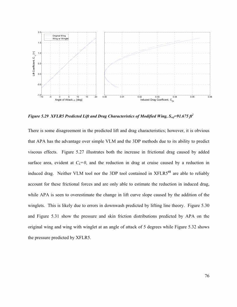
76
Figure 5.29 XFLR5 Predicted Lift and Drag Characteristics of Modified Wing, Sref=91.675 ft2
There is some disagreement in the predicted lift and drag characteristics; however, it is obvious
that APA has the advantage over simple VLM and the 3DP methods due to its ability to predict
viscous effects. Figure 5.27 illustrates both the increase in frictional drag caused by added
surface area, evident at CL=0, and the reduction in drag at cruise caused by a reduction in
induced drag. Neither VLM tool nor the 3DP tool contained in XFLR541 are able to reliably
account for these frictional forces and are only able to estimate the reduction in induced drag,
while APA is seen to overestimate the change in lift curve slope caused by the addition of the
winglets. This is likely due to errors in downwash predicted by lifting line theory. Figure 5.30
and Figure 5.31 show the pressure and skin friction distributions predicted by APA on the
original wing and wing with winglet at an angle of attack of 5 degrees while Figure 5.32 shows
the pressure predicted by XFLR5.
-10 -5 0 5 10 15 20-1.0
-0.5
0.0
0.5
1.0
1.5
2.0
Angle of Attack, [deg]
Lift
Coe
ffici
ent
, CL [~
]
0.00 0.01 0.02 0.03 0.04 0.05 0.06
Induced Drag Coefficent, CDi
Original WingWing w/ Winglet
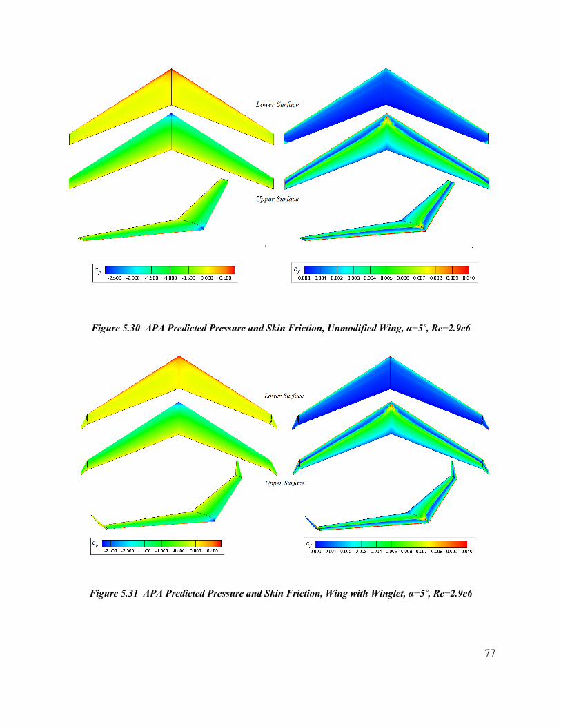
77
Figure 5.30 APA Predicted Pressure and Skin Friction, Unmodified Wing, α=5˚, Re=2.9e6
Figure 5.31 APA Predicted Pressure and Skin Friction, Wing with Winglet, α=5˚, Re=2.9e6

78
Figure 5.32 XFLR5 Predicted Pressure and Skin Friction, α=5˚, Re=2.9e6
The exaggerated downwash caused by the lifting line theory in APA causes increased angle of
attack at the wing root. This results in the low pressure area at the wing apex shown in Figure
5.30 and Figure 5.31, otherwise there is reasonable agreement between the pressure distributions
predicted using APA and 3DP tool in XFLR541. While the skin friction distributions pictured in
these figures are based solely on the XFOIL results, it does provide some limited insight into the
transition location of the boundary layer along the wing. This is evidenced by rapid change in
skin friction with a small change in chord. In Figure 5.30 and Figure 5.31 this is evidenced by
the change from blue to green hue in the skin friction plots.
79
6. Conclusions and Recommendations
This section summarizes the conclusions and recommendations reached as part of the current
effort. This includes recommendations for future expansion, research or validation.
6.1 Conclusions
The methods explained in this work and employed in the accompanying MATLAB6 code
provide a way to estimate distributed aerodynamics loads, basic aerodynamic properties, and
pressure/friction distributions on wings of nearly arbitrary shape in low subsonic compressible
flow. This is done with varying degrees of accuracy depending on the shape of the planform
being analyzed, operating condition, and many other variables. The biggest limiting factor of
this method is the selected lifting line theory. This requires corrections for shift in aerodynamic
center that exaggerate the predicted downwash and ultimately affect the distributed loads.
Nevertheless, it is shown to model the elliptic wing problem with considerable accuracy as well
as the rectangular wing problem with less agreement for the swept wing case and decidedly
unreliable results when applied to wings with control surfaces.
For the rectangular wing case, the biggest errors are seen to be caused by blunt wing tips which
cannot be modeled by this or any other lifting line theory without some form of assumption or
adjustment. There are also errors induced by the airfoil data which is limited by the accuracy of
the XFOIL calculations. These limitations are well known and serve to reduce the applicability
of the current method, but it still provides a reasonably accurate and adaptable way to analyze
wing loading.
The errors induced in the swept wing analysis are mostly due to the exaggerated downwash
prediction that rolls out of the lifting line analysis. This is caused by the application of the
80
regular or extended tangent approximations which are used to mitigate numerical singularities in
the lifting line formulation. This suggests that perhaps this method of shifting aerodynamic
centers is not the best approach, especially if spanwise loading is of interest. That being said, the
methods presented here are shown to make very accurate and reliable calculations of the lift-drag
relationship illustrated by the various drag polars for swept wing presented above.
There is also a notable limitation of the lifting line theory that is worth mentioning, specifically
the handling of the inviscid wake. This is accomplished by the infinite trailing tails of the vortex
system which point in the direction of the freestream. However, in reality this inviscid wake
leaves the trailing edge of the planform at an angle dictated by the local airfoil geometry as
required by the Kutta-condition at which point it begins bend toward the freestream. This
discrepancy in the wake geometry can impact the downwash distribution, particularly for cases
like wing with control surface or cranked wing. Since this is a problem for most lifting line
theories, it may be one that cannot be solved with the approach applied here.
The methods for distributing pressure and frictional forces explained are also somewhat accurate
for cases without control surface deflection but are again limited by the accuracy of the lifting-
line theory. However, in cases with control surface deflection some odd results are observed.
Further research is needed in this area to determine if this is inherent to the interpolation
procedure or if it is somehow a product of the lifting-line theory.
6.2 Recommendations
Based on the results and conclusion presented here, the following recommendations can be
made. First and foremost, is the errors inherent to the lifting line theory and tangent
approximations must be addressed. This will improve accuracy of the pressure and shear
81
distributions as well as the predicted lift and drag characteristics beyond what has already been
documented. This may require choosing a completely new lifting line theory or simply
employing a spline interpolation to smooth over the area affected by the singularity. Further
improvements to the lifting line theory might include accounting for fuselage effects and systems
of interacting lifting surfaces.
This may also be accomplished by tweaking the extended tangent approximation in some way,
but it is not clear how this might be accomplished. Furthermore, CFD or experimental validation
of the extended tangent approximation as applied to the cranked wing case is needed to truly
validate this method. However, the extended tangent approximation does in fact provide a
reliable way to mitigate the effects of the singularities of the lifting-line theory, exaggerated
downwash errors aside.
It would be possible to further expand the applicability of these methods by applying MSES18
which is capable of multi-element airfoil analysis. This would allow for the anlaysis of
planforms with control surfaces such as Krueger flaps, single and double-slotted flaps, leading
edge slats, and many more. Unfortunately, increases in accuracy of the airfoil data would require
complicated and time consuming CFD analysis. Yet, it is certainly possible to provide input
options in APA which allow for use of experimental data if it were available.
It might also be possible to extend these methods to the transient case by applying a dynamic
stall model and a time marching routine. However, this should be considered only after
addressing the other sources of error which have been discussed either through the
recommendations offered or through some other means.

82
7. References
1. Brown, M, Kaushik, B., and Anemaat, W.A., ‘Planform Load Distribution Mapping for Straight Tapered Wings with Linear Twist’, AIAA-2012-0396, 50th AIAA Aerospace Sciences Meeting, Jan 9-12, 2012, Nashville, TN.
2. Brown, M. and Carroll, J., ‘BEM + PFDM’, In-House MATLAB Code, DARcorporation, Lawrence, KS., 66049, ©2012.
3. Roskam, J., ‘Airplane Design, Parts II & VI,’ DARcorporation, Lawrence, KS, 66049, ©2005.
4. Raymer, D., ‘Aircraft Design-A Conceptual Approach’, AIAA Education Series, Air Force Institute of Technology, Wright Patterson Air Force Base, Ohio, ©1992
5. Torrenbeek, E., ‘Synthesis of Subsonic Airplane Design,’ Delft University Press, Delft, The Netherlands, ©1982.
6. ‘MATLAB R2011a, Student Version’, The MathWorks, Inc., Natick, MA., ©2011.
7. Anderson., J.D., ‘Fundamentals of Aerodynamics’, 4th Edition, McGraw-Hill, New York, NY, ©2007.
8. McCormick, W.B., ‘Aerodynamics, Aeronautics, and Flight Mechanics,’ 2nd Edition, Wiley & Sons, Hoboken, NJ, ©1994.
9. Moran, J., ‘An Introduction to Theoretical and Computational Aerodynamics,’ Dover Publications, Inc., Mineola, NY, ©1984.
10. Yates, J.E., ‘Viscous Thin Airfoil Theory,’ Aeronautical Research Associates of Princeton (ARAP), Inc., Princeton, NJ, ©1980.
11. Eppler, R., and Somers, D.M., ‘A Computer Program for the Design and Analysis of Low-Speed Airfoils’. NASA TM-80210, 1980.
12. Hepperle, M., ‘Javafoil’, Java Script for Airfoil Analysis, www. mh-aerotools.de/airfoils/javafoil.htm, ©2006.
13. Thwaites, B., ‘Approximate Calculation of the Laminar Boundary Layer,’ Aeronaut. Q. 1, 245-280,©1949
14. Drela, M., ‘XFOIL: An Analysis and Design System for Low Reynolds Number Airfoils’, Massachusetts Institute of Technology, Department of Aeronautics and Astronautics, Cambridge, MA, ©1989.
15. Drela, M., ‘Design and Optimization Methods for Multi-Element Airfoils,’ AIAA 93-0969, AIAA Aerospace Design Conference, Irvine, CA, ©1993.

83
16. Drela, M. and Giles, M.B., ‘Viscous-Inviscid Analysis of Transonic and Low Reynolds Number Airfoils,’ AIAA 9789-427, AIAA Journal, Vol. 25, No. 10, pp 1347-1355, October, 1987.
17. Drela, M., ‘XFOIL v6.9,’ Massachusetts Institute of Technology, Department of Aeronautics and Astronautics, Cambridge, MA, ©2001.
18. Drela, M., ‘MSES v3.05’, Massachusetts Institute of Technology, Department of Aeronautics and Astronautics, Cambridge, MA, ©2007.
19. Lanchester, F.W., ‘Aerodynamics: Constituting the First Volume of a Complete Work on Aerial Flight,’ A. Constable & Co., Ltd., London, UK. ©1907.
20. Prandtl, L., ‘Tragflügeltheorie,’ Königliche Gesellschaft der Wissenschaften zu Göttingen, ©1918.
21. Saffman, P.G., ‘Vortex Force and Bound Vorticity,’ Vortex Dynamics, Cambridge University Press, Cambridge, England, UK, ©1992.
22. Multhopp, H., ‘Methods for Calculating the Lift Distribution of Wings (Subsonic Lifting Surface Theory),’ ARC Technical Report, R&M no. 2884, Aeronautical Research Council, London, England, UK, 1955.
23. Rasmussen, M.L. and Smith, D.E., ‘Lifting-Line Theory for Wings Arbitrary Shaped Wings,’ Journal of Aircraft, Vol. 36, No. 2, ©1999, pp. 340-348.
24. Blackwell, J.A., ‘A Finite-Step Method for Calculation of Theoretical Load Distributions for Arbitrary Lifting Surface Arrangements at Subsonic Speeds,’ NASA TN D-5335, National Aeronautics and Space Administration, Washington D.C., ©1969.
25. DeYoung, J., ‘Nonplanar Wing Load-Line and Slender Wing Theory,’ NASA CR-2864, National Aeronautics and Space Administration, Washington D.C., ©1977.
26. Kratz, J. and Plotkin, A., ‘Low Speed Aerodynamics’, Cambridge University Press, Cambridge, England, UK, ©1991.
27. Phillips, W.F. and Snyder, D.O., ‘Modern Adaptation of Prandtl’s Lifting Line,’ Journal of Aircraft, Vol. 37, No. 4, ©2000.
28. Weber, J. and Brebner, G.G., ‘Low Speed Tests on 45-deg Swept-Back Wings. Part 1: Pressure Measurements on Wings of Aspect Ratio 5,’ Aeronautical Research Council, RM-2882, London, England, UK, ©1958.
29. Hall, I.M. and Rogers, E.W.E, ‘Experiments with a Tapered Sweptback Wing of Warren 12 Planform at Mach Numbers between 0.6 and 1.6,’ Aeronautical Research Council, RM-3271, London, England, UK, ©1962.

84
30. Kuchemann, D., ‘A Simple Method for Calculating the Span and Chordwise Loading of Straight and Swept Wings of any Given Aspect Ratio at Subsonic Speeds’, Aeronautical Research Council, RM-2935, London, England, UK, ©1956.
31. Phillips, W.F. and Hunsaker, D.F., ‘Estimating the Subsonic Aerodynamic Center and Moment Components for Swept Wings,’ Journal of Aircraft, Vol. 45, No. 3, ©2008.
32. DeYoung, J., ‘Vortex Lattice Utilization,’ NASA SP-405, National Aeronautics and Space Administration, Washington D.C., ©1976.
33. Falkner, V.M., ‘The Accuracy of Calculations Based on the Vortex Lattice Theory,’ Aeronautical Research Council, No. 9621, London, England, UK, ©1946.
34. Lan, C.E., ‘VORSTAB: A Program for Calculating Lateral-Directional Stability Derivatives with Vortex Flow Effect,’ NASA CR-172501, National Aeronautics and Space Administration, Washington D.C., ©1985.
35. Melin, T., ‘Tornado v135’, Vortex Lattice Method Software, Red Hammer Consulting, ©2010.
36. Drela, M. and Youngren, H., ‘AVL: Athena Vortex Lattice v3.32’, Massachusetts Institute of Technology, Cambridge, MA, ©2012.
37. Anon., ‘VSAERO’, 3D Panel Software, Analytical Methods, Inc., Richmond, WA, ©2013.
38. Tu, J., Yeoh, G.H., and Liu, C., ‘Computational Fluid Dynamics: A Practical Approach’, Elsevier, Burlington, MA, ©2008.
39. Anon., ‘Fluent,’ CFD Software, ANSYS Corp., Canonsburg, PA, ©2013.
40. Anon., ‘STAR-CCM+’, CFD Software, CD-Adapco, Melville, NY, ©2013.
41. Anon., ‘XFLR5 v6.09.01 beta’, GNU General Public License, ©2013.
42. Sivells, J.C. and Neely, R.H., ‘Method for Calculating Wing Characteristics by Lifting Line Theory Using Non-Linear Section Lift Data,’ NACA TN 1269, National Advisory Commite for Aerounautics, ©1947.
43. Scherrer, M., ‘Integral Method over a Wing for Experimental and Xfoil Results: MIAReX v0.9’, MATLAB Code, ©2004.
44. Barlow, J.B., Rae, W.H., and Pope, A., ‘Low-Speed Wind Tunnel Testing,’ 3rd Edition, Wiley-Interscience, Hoboken, NJ, ©1999.
45. Anon., Wind Tunnel Model Photograph, www.darcorp.com/Aeronautical_Engineering/Projects/ show.php?show=busjet, October, 2013.
85
46. Drela, M. and Youngren, H., ‘XFOIL 6.9 USER PRIMER’, Massachusetts Institute of Technology, Cambridge, MA, ©2001.
47. Tangler, J.L. and Kocurek, J.D., ‘Wind Turbine Post-Stall Airfoil Performance Characteristics Guidelines for Blade-Element Momentun Methods,’ NREL/CP-500-38456, AIAA/NREL, ©2005.
48. Abbot, I.H. and Von Doenhoff, A.E., ‘Theory of Wing Sections,’ Dover Publications, Inc., New York, NY. ©1949.
49. Kolbe. C.D. and Boltz, F.W., ‘The Forces and Pressure Distribution at Subsonic Speeds on a Plane Wing Having 45˚ Sweepback, Aspect Ratio of 3, and a Taper Ratio of 0.5,’ NACA RM-451G31, National Advisory Committee for Aeronautics, ©1951.
50. Graham, R.R., ‘Low-Speed Characteristics of a 45˚ Sweptback Wing of Aspect Ratio 8 from Pressure Distribution and Force Tests at Reynolds Numbers from 1,500,000 to 4,800,000,’ NACA RM-L51H13, National Advisory Committee for Aeronautics, ©1951.
51. Anon., ‘Tecplot 360 2010 R1,’ Tecplot, Inc., Bellevue, WA, ©2010.
52. McAlister, K.W. and Takahasi, R.K., ‘NACA 0015 Wing Pressure and Trailing Vortex Mesurements,’ NASA TP 3151, National Aeronautics and Space Administration,. Washington, D.C., ©1991.
53. Jacobs, W., ‘Pressure-Distribution Measurements on Unyawed Swept-Back Wings,’ NACA TM 1164, National Advisory Committee for Aeronautics, Washington, D.C., ©1947.
54. Johnson, H.S. and Hagerman, J.R., ‘Wind-Tunnel Investigation at Low Speed of An Unswept Untapered Semispan Wing of Aspect Ratio 3.13 Equiped with Various 25-Percent-Chord Plain Flaps,’ NACA TN 2080, National Advisory Committee for Aeronautics, Washington, D.C., ©1950.

86
Appendix A-MATLAB Code
function [Aero,Geo,OpCon,CalcSet,VarVec,PostPro,Results]=AdvancedPlanformAnalysis(filename,buff) %% Introduction % By: Matt Brown % Created Fall 2012 - Fall 2013 % % Submitted to the Department of Aerospace Engineering and the Faculty of the Graduate School of % Engineering at the University of Kansas in Partial Fulfillment of the Requirements for the Degree % of Master of Science in Aerospace Engineering. % % Inputs: All inputs are made through spreadsheet 'filename'. Planform % definitions are made through the classic cranked wing method and assumes a linear change in properties % from root to tip of each panel. Controls for postprocessing and calculation are defined in the % spreadsheet. % % Panel ID: Integer denoting panel of symetric wing planform starting at the % root (ID=1) and increasing up to N panels. % % Panel Quarter Chord Positions: X,Y,Z locations (in ft) of the panel root and % tip quarter chord. All itermediate points are assumed to lie linearly % between the root and tip. Ensure that the root of each new panel is % the same as the tip of the preceeding panel. % % Panel Geometry: Defines control surface chord ratios, root and tip % chords, incidence and twist for each panel. % % c_f/c: Control surface chord ratio, number between 0 and 1 % representing the % of the airfoil deflected by the control % surface. % % c_r, c_t: Panel Root and Tip Chord in ft % % i_r: Panel root incidence in degrees. % % epsilon_p: Panel twist in degrees. % % Airfoils (Root and Tip): These are names of airfoils either: % a) stored in the Airfoil Database in proper format % b) a 4 or 5 digit NACA airfoil of entered in the form 'NACA XXXX' or 'NACA XXXXX'. % % Surface Definitions: Defines the control surface type and node density % for each panel. % % Ctrl Surf: Dropdown list defines a constant chord ratio aileron or plain flap

87
% that covers the entire span of the panel. For a clean section, % select clean % % Node Den: Allows you to modify the number of control points on % individual panels. This is a number greater than 0. % Ex. 26 Nodes/Panel*0.5 = 13 Panels % % Atmospheric Conditions: Defines the properties of the atmosphere used in various phases of the calculations. % % P_o: Absolute Pressure in psf % % T_o: Temperature in R % % rho_o: Density in slug/ft^3 % % R: Gas Constat (use 1716.37 for Air) % % gamma: Ratio of Specific Heats (use 1.4 for Air) % % nu: Kinematic Viscosity in ft^2/s % % Flight Condition: Defines the Sspeed, Angle of Attack, Sideslip Angle % and Control Surface Deflection Angles % % KTAS: True Air Speed in Knots % % alpha: Angle of Attack in degrees % % beta: Angle of Side Slip in degrees % % delta_a: aileron deflection angle in degrees % % delta_f: flap deflection angle in degrees % % Calculation Settings: Defines the Solver Settings for APA % % Tolerance: Convergence tolerance for Lifting Line Theory % % Relaxation: Relaxation Factor for Lifting Line Theory % % Max Iterations: Maximum Iterations for Lifting Line Theory % % Number of Elements/Panel: Number of Elements to place on each % panel. Adjust individual panels using the Node Density % variable. % % Chord Distribution: Dropdown list with Linear and Elliptic % Options. When using Elliptic option, chord distribution is % based soley on root chord input of panel 1. Define all other % chords equal to the root chord for best xfoil results. When % using Linear Function, define each panel root and tip with the % appropriate chord based on your CAD or conceptual model. % % Transition Criteria: Dropdown list which defines xfoil
88
% transition criteria based on operating condition. Default % setting should be Normal Conditions which gives Ncrit=9. % % Compressibility Corrections: Dropdown list with On/Off. When % turned On, all xfoil results are corrected using standard xfoil % compressibility correction. When turned off, speed only effects % Reynolds number which impacts transition but not magnitude of % pressure. % % Station Plot Settings: Defines the options for the station plots. % % Station Locations: An input string wich defines all span % stations between -1 and 1. For example: [0,0.1,0.3] would plot % the selected distributions at 2y/b=0, 0.1 and 0.3 % % Processing Options: On/Off dropdown lists to select plots and % solvers for postprocessing. See description in spreadsheet for % details. % % Outputs: All results are contained in the data structure Results and % ploted based on the selected options. Aditional on screen results are % also given. % %% Initialize Buffer if Called if strcmp(buff,'On') clc clear Aero Geo OpCon CalcSet PostPro Results VarVec format long end disp(' Welcome to Advanced Planform Analysis v1.0') disp('========================================================') %% Load Input and Calculate Endpoints str=horzcat('Loading... ',filename); disp(str) [Geo,OpCon,CalcSet,PostPro]=fLoadFile(filename); [Geo]=fEndPts(Geo); %% Calculate Section Aerodynamics str=horzcat('Calculating... ','Section Aerodynamics'); disp(str) [Geo,Aero]=fAero(Geo,OpCon,CalcSet); %% Calculate Variables str=horzcat('Calculating... ','Planform Variables'); disp(str) [VarVec,OpCon,Geo]=fVariables(Geo,Aero,OpCon,CalcSet); %% Run Selected Solver(s) oi=OpCon.Input; Results.Type1.poston='off'; Results.Type2.poston='off';
89
Results.Type3.poston='off'; if strcmp(PostPro.Solver.Type1,'On')==1 t1=tic; str=horzcat('Solving... ','Type 1 Analysis'); disp(str) u1=sqrt((oi.U1*1.68780986)^2/(1+tand(oi.Alpha)^2+tand(oi.Beta)^2))*[1;tand(oi.Beta);-tand(oi.Alpha)]; vinf=u1/(oi.U1*1.68780986); Results.Type1.vinf=vinf; [ Results.Type1.v ] = fveolocity( VarVec,vinf ); [ Results.Type1.G1,Results.Type1.iter,Results.Type1.conv ] = fsolveG(vinf,CalcSet,VarVec,Aero,Results.Type1.v ); Results.Type1.time=toc(t1); if strcmp(Results.Type1.conv,'fail')==1 disp('!!!Failed Convergence-Type 1 Analysis. Please Modify Input!!!') Results.Type1.poston='off'; else disp(horzcat('Converged... Type 1 Analysis.')) disp(horzcat(' CPU Time: ',num2str(Results.Type1.time,3),' s')) Results.Type1.poston='on'; end end if strcmp(PostPro.Solver.Type2,'On')==1 t1=tic; str=horzcat('Solving... ','Type 2 Analysis'); disp(str) a=[-6,-3,0,3,6]; clear vinf v G1 iter conv for i=1:numel(a) u1=sqrt((oi.U1*1.68780986)^2/(1+tand(a(i))^2+0))*[1;0;-tand(a(i))]; vinfi=[u1/(oi.U1*1.68780986)]; [ vi ] = fveolocity( VarVec, vinfi); [ G1i,iter(i),convi ] = fsolveG(vinfi,CalcSet,VarVec,Aero,vi ); end k=1; for i=1:numel(a) if strcmp(convi,'pass') pass(i)=1; Results.Type2.vinfk=vinfi; Results.Type2.G1k=G1i; Results.Type2.iter(k)=iter(i); Results.Type2.convk=convi; Results.Type2.AoA(k)=a(i); Results.Type2.vk=vi; k=k+1; else pass(i)=0; end end Results.Type2.time=toc(t1); if sum(pass)<=1 disp('!!!Failed Convergence-Type 2 Analysis. Please Modify Input!!!') Results.Type2.poston='off';
90
else disp(horzcat('Converged... Type 2 Analysis')) disp(horzcat(' CPU Time: ',num2str(Results.Type2.time,3),' s')) Results.Type2.poston='on'; end end if strcmp(PostPro.Solver.Type3,'On')==1 t1=tic; str=horzcat('Solving... ','Type 3 Analysis'); disp(str) a=[-10:20]; clear vinf v G1 iter conv for i=1:numel(a) u1=sqrt((oi.U1*1.68780986)^2/(1+tand(a(i))^2+0))*[1;0;-tand(a(i))]; vinfi=u1/(oi.U1*1.68780986); [ vi ] = fveolocity( VarVec, vinfi); [ G1i,iter(i),convi ] = fsolveG(vinfi,CalcSet,VarVec,Aero,vi ); end k=1; for i=1:numel(a) if strcmp(convi,'pass') pass(i)=1; Results.Type3.vinfk=vinfi; Results.Type3.G1k=G1i; Results.Type3.iter(k)=iter(i); Results.Type3.convk=convi; Results.Type3.AoA(k)=a(i); Results.Type3.vk=vi; k=k+1; else pass(i)=0; end end Results.Type3.time=toc(t1); if sum(pass)<=10 disp('!!!Failed Convergence-Type 3 Analysis. Please Modify Input!!!') Results.Type3.poston='off'; else disp(horzcat('Converged... Type 3 Analysis.')) disp(horzcat(' CPU Time: ',num2str(Results.Type3.time,4),' s')) Results.Type3.poston='on'; end end %% Post Processing [Geo]=fPlanform(Geo,VarVec); % Type 1 Analysis if strcmp(Results.Type1.poston,'on') % set variables v=Results.Type1.v; vinf=Results.Type1.vinf; G=Results.Type1.G1; % Solve for AOA & V Dist

91
[ alpha_i,alpha_inf,alpha,V,Vdist ] = fPost_alpha( OpCon, VarVec, v, vinf,G); % Solve Circulation and Cl, Cdi dist [ Gamma,cl,cdi,clnorm,cdinorm ] = fPost_Gamma(Geo, OpCon,VarVec, v, vinf, G, alpha_i); % Solve for Coeff Distributions [ CoeffDist ] = fPost_Aero(Aero,VarVec,alpha); % Get AC locus [ xyzac,dxac,dzac ] = fPost_xzac(VarVec); % Solve for Forces and Moments [ f,F,m,M ] = fPost_forces( OpCon,VarVec,CoeffDist,Gamma,Vdist,v,vinf); F.L=-F.t(3)*cosd(OpCon.Input.Alpha)-F.t(1)*sind(OpCon.Input.Alpha); F.D=-F.t(3)*sind(OpCon.Input.Alpha)+F.t(1)*cosd(OpCon.Input.Alpha); % Solve for Planform Coeff [ Coeff ] = fPost_Coeff( F,M,OpCon,Geo,OpCon.Input.Alpha ); % Display Results fPost_Type1( F,M,Coeff ); % Output Data Results.Type1.alpha=alpha; Results.Type1.alpha_inf=alpha_inf; Results.Type1.alpha_i=alpha_i; Results.Type1.CoeffDist=CoeffDist; Results.Type1.Gamma=Gamma; Results.Type1.cl=cl; Results.Type1.clnorm=clnorm; Results.Type1.cdi=cdi; Results.Type1.cdinorm=cdinorm; Results.Type1.xyzac=xyzac; Results.Type1.dxac=dxac; Results.Type1.dzac=dzac; Results.Type1.f=f; Results.Type1.m=m; % Plots if strcmp(PostPro.LLTplots.AOA,'On')==1 createfigure1(VarVec.etam, [ alpha; alpha_i; alpha_inf ]); end if strcmp(PostPro.LLTplots.clcd2d,'On')==1 rtc=Results.Type1.CoeffDist; createfigure2(VarVec.etam, [ rtc.cl2d ; rtc.cm2d ], [ rtc.cd2d ; rtc.cdp2d ; rtc.cdf2d ]); end if strcmp(PostPro.LLTplots.cnca2d,'On')==1 rtc=Results.Type1.CoeffDist; createfigure3(VarVec.etam, [ rtc.cn2d ; rtc.cm2d ], [ rtc.ca2d ; rtc.cap2d ; rtc.caf2d ]); end if strcmp(PostPro.LLTplots.Gclcd,'On')==1 rt=Results.Type1; createfigure4(VarVec.etam, rt.Gamma, rt.cl, rt.cdi ); end if strcmp(PostPro.LLTplots.fmxyz,'On')==1 rtf=Results.Type1.f; rtm=Results.Type1.m; createfigure5(VarVec.etam, [ rtf.p(:,1),rtf.f(:,1) ,rtf.t(:,1) ],...

92
[ rtf.p(:,2),rtf.f(:,2) ,rtf.t(:,2) ], [ rtf.p(:,3),rtf.f(:,3) ,rtf.t(:,3) ]) createfigure6(VarVec.etam, [ rtm.p(:,1),rtm.f(:,1) ,rtm.t(:,1) ],... [ rtm.p(:,2),rtm.f(:,2) ,rtm.t(:,2) ], [ rtm.p(:,3),rtm.f(:,3) ,rtm.t(:,3) ]) end if strcmp(PostPro.LLTplots.dxzac,'On')==1 rt=Results.Type1; createfigure11(VarVec.etam, [ rt.dxac;rt.dzac ], rt.xyzac(:,1), rt.xyzac(:,2), rt.xyzac(:,3)) end if strcmp(PostPro.Stationplots.cpf,'On')==1 for i=1:numel(PostPro.Station.Location) [ xi,cpi,cfi,pi,taui ] = fPost_getcpf( PostPro.Station.Location(i),VarVec, alpha,Aero,OpCon ); createfigure12(xi, cpi, cfi,horzcat(' 2y/b = ',num2str(PostPro.Station.Location(i),'%3.3f'))) end Results.Type1.Station.x=x; Results.Type1.Station.cp=cp; Results.Type1.Station.cf=cf; end if strcmp(PostPro.Stationplots.ptau,'On')==1 for i=1:numel(PostPro.Station.Location) [ xi,cpi,cfi,pi,taui ] = fPost_getcpf( PostPro.Station.Location(i),VarVec, alpha,Aero,OpCon ); createfigure13(xi, pi, taui,horzcat(' 2y/b = ',num2str(PostPro.Station.Location(i),'%3.3f'))) end Results.Type1.Station.x=x; Results.Type1.Station.p=p; Results.Type1.Station.tau=tau; end afid=1:VarVec.AFID(end); if strcmp(PostPro.Surfplots,'On')==1 for i=1:VarVec.AFID(end) % assemble xyz and cp p cf tau for each panel [ xyzi,cpi,pi,cfi,taui,Npts(i),Nelem(i),Naf(i)] = fPost_PanelData( OpCon,Geo,Aero,VarVec,afid(i),alpha ); Results.Type1.Surf.xyzi=xyzi; Results.Type1.Surf.cpi=cpi; Results.Type1.Surf.cfi=cfi; Results.Type1.Surf.pi=pi; Results.Type1.Surf.taui=taui; end fPost_Tecplot( xyz,cp,cf,p,tau,Nelem,Npts,Naf,filename ); end end % Type 2 Analysis if strcmp(Results.Type2.poston,'on') % set variables for i=1:numel(Results.Type2.AoA) v=Results.Type2.vi; vinf=Results.Type2.vinfi;

93
G=Results.Type2.G1i; % Solve for AOA & V Dist [ alpha_i,alpha_inf,alpha,V,Vdist ] = fPost_alpha( OpCon, VarVec, v, vinf,G); % Solve Circulation and Cl, Cdi dist [ Gamma,cl,cdi,clnorm,cdinorm ] = fPost_Gamma(Geo, OpCon,VarVec, v, vinf, G, alpha_i); % Solve for Coeff Distributions [ CoeffDist ] = fPost_Aero(Aero,VarVec,alpha); % Solve for Forces and Moments [ f,F,m,M ] = fPost_forces( OpCon,VarVec,CoeffDist,Gamma,Vdist,v,vinf); % Solve for Planform Coeff [ Coeff ] = fPost_Coeff( F,M,OpCon,Geo,Results.Type2.AoA(i) ); % Assemble Data CL(i)=Coeff.CL; CD(i)=Coeff.CD; Cm(i)=Coeff.Cm; end % Output Data p=polyfit(Results.Type2.AoA,CL,1); Results.Type2.CLo=p(2); Results.Type2.CLalpha=p(1)*180/pi; Results.Type2.Alpha0=-p(2)/p(1); p=polyfit(Results.Type2.AoA,Cm,1); Results.Type2.Cmalpha=p(1)*180/pi; Results.Type2.Cm0=p(1)*Results.Type2.Alpha0+p(2); p=polyfitn(CL,CD,'x^2','constant'); Results.Type2.CDo=p.Coefficients(2); Results.Type2.BCD=p.Coefficients(1); fPost_Type2( Results.Type2,Geo.Planform.AR ) end % Type 3 Analysis if strcmp(Results.Type3.poston,'on') % set variables for i=1:numel(Results.Type3.AoA) v=Results.Type3.vi; vinf=Results.Type3.vinfi; G=Results.Type3.G1i; % Solve for AOA & V Dist [ alpha_i,alpha_inf,alpha,V,Vdist ] = fPost_alpha( OpCon, VarVec, v, vinf,G); % Solve Circulation and Cl, Cdi dist [ Gamma,cl,cdi,clnorm,cdinorm ] = fPost_Gamma(Geo, OpCon,VarVec, v, vinf, G, alpha_i); % Solve for Coeff Distributions [ CoeffDist ] = fPost_Aero(Aero,VarVec,alpha); % Solve for Forces and Moments [ f,F,m,M ] = fPost_forces( OpCon,VarVec,CoeffDist,Gamma,Vdist,v,vinf); % Solve for Planform Coeff [ Coeff ] = fPost_Coeff( F,M,OpCon,Geo,Results.Type3.AoA(i) ); % Assemble Data Results.Type3.CL(i)=Coeff.CL; Results.Type3.CD(i)=Coeff.CD; Results.Type3.CDi(i)=Coeff.CDi; Results.Type3.Cm(i)=Coeff.Cm;

94
Results.Type3.Fx(i)=F.t(1); Results.Type3.Fy(i)=F.t(2); Results.Type3.Fz(i)=F.t(3); end k=find(Results.Type3.AoA>=10); p=polyfit(Results.Type3.CL(1:k),Results.Type3.CD(1:k),5); % Output results Results.Type3.CDo=p(6); Results.Type3.BCD1=p(5); Results.Type3.BCD2=p(4); Results.Type3.BCD3=p(3); Results.Type3.BCD4=p(2); Results.Type3.BCD5=p(1); fPost_Type3( Results.Type3 ) % Plots if strcmp(PostPro.Planformplots.ClvAoA,'On')==1 rt=Results.Type3; createfigure7(rt.AoA, rt.CL) end if strcmp(PostPro.Planformplots.CdivAoA,'On')==1 rt=Results.Type3; createfigure8(rt.AoA, [rt.CD;rt.CDi] ) end if strcmp(PostPro.Planformplots.CmvAoA,'On')==1 rt=Results.Type3; createfigure9(rt.AoA, rt.Cm) end %% if strcmp(PostPro.Planformplots.ClvCd,'On')==1 for i=1:numel(Results.Type3.CL) Results.Type3.CDpolar(i)=Results.Type3.CDo+Results.Type3.BCD1*Results.Type3.CL(i)+Results.Type3.BCD2*Results.Type3.CL(i)^2+... Results.Type3.BCD3*Results.Type3.CL(i)^3+Results.Type3.BCD4*Results.Type3.CL(i)^4+... Results.Type3.BCD5*Results.Type3.CL(i)^5; end createfigure10(Results.Type3.CD, Results.Type3.CL, Results.Type3.CDi, Results.Type3.CDpolar) end end disp('========================================================') end %% Sub-Functions function createfigure1(X1, YMatrix1) %CREATEFIGURE(X1,YMATRIX1) % X1: vector of x data % YMATRIX1: matrix of y data % Auto-generated by MATLAB on 11-Oct-2013 12:40:48 ymax=ceil(max(unique(YMatrix1)))+1; ymin=floor(min(unique(YMatrix1)))-1; % Create figure
95
figure1 = figure('Color',[0.800000011920929 0.800000011920929 0.800000011920929],'Position',[10 520 1600 300],'Name','Angle of Attack Distribution'); % Create axes axes1 = axes('Parent',figure1,'YGrid','on','XGrid','on',... 'Position',[0.05 .175 0.85 0.75]); box(axes1,'on'); hold(axes1,'all'); % Create multiple lines using matrix input to plot plot1 = plot(X1,YMatrix1,'Parent',axes1); ylim([ymin ymax]); set(plot1(1),'Marker','o','DisplayName','\alpha'); set(plot1(2),'Marker','v','DisplayName','\alpha_i'); set(plot1(3),'Marker','square','DisplayName','\alpha_\infty'); % Create xlabel xlabel('Span Location, \eta = 2y/b'); % Create ylabel ylabel('Angle of Attack, \alpha [deg]'); % Create legend legend1 = legend(axes1,'show'); set(legend1,'Location','NorthEastOutside'); % Resize the axes in order to prevent it from shrinking. set(axes1,'Position',[0.05 .175 0.85 0.75]); end function createfigure2(X1, YMatrix1, YMatrix2) %CREATEFIGURE(X1,YMATRIX1,YMATRIX2) % X1: vector of x data % YMATRIX1: matrix of y data % YMATRIX2: matrix of y data % Auto-generated by MATLAB on 11-Oct-2013 15:22:09 % Create figure figure1 = figure('Color',[0.800000011920929 0.800000011920929 0.800000011920929],'Position',[10 220 1600 600],'Name','2D Lift and Drag Distribution'); % Create axes axes1 = axes('Parent',figure1,'YGrid','on','XGrid','on',... 'Position',[0.1 0.58 0.83 0.35]); box(axes1,'on'); hold(axes1,'all'); % Create multiple lines using matrix input to plot plot1 = plot(X1,YMatrix1,'Parent',axes1); set(plot1(1),'Marker','o','DisplayName','c_l_(_2_D_)'); set(plot1(2),'Marker','square','DisplayName','c_m_(_2_D_)'); % Create ylabel ylabel('Lift and Moment','Coefficients, c_l & c_m [~]');
96
% Create axes axes2 = axes('Parent',figure1,'YGrid','on','XGrid','on',... 'Position',[0.1 0.13 0.75 0.35]); box(axes2,'on'); hold(axes2,'all'); % Create multiple lines using matrix input to plot plot2 = plot(X1,YMatrix2,'Parent',axes2); set(plot2(1),'Marker','o','DisplayName','c_d_(_2_D_)'); set(plot2(2),'Marker','square','DisplayName','c_d_p _(_2_D_)'); set(plot2(3),'Marker','v','DisplayName','c_d_f _(_2_D_)'); % Create ylabel ylabel('Drag Coefficients, c_d [~]'); % Create xlabel xlabel('Span Location, \eta = 2y/b [~]'); % Create legend legend1 = legend(axes1,'show'); set(legend1,'Location','NorthEastOutside'); % Create legend legend2 = legend(axes2,'show'); set(legend2,'Location','NorthEastOutside'); % Resize the axes in order to prevent it from shrinking. set(axes2,'Position',[0.1 0.13 0.75 0.35]); end function createfigure3(X1, YMatrix1, YMatrix2) %CREATEFIGURE(X1,YMATRIX1,YMATRIX2) % X1: vector of x data % YMATRIX1: matrix of y data % YMATRIX2: matrix of y data % Auto-generated by MATLAB on 11-Oct-2013 15:22:09 % Create figure figure1 = figure('Color',[0.800000011920929 0.800000011920929 0.800000011920929],'Position',[10 220 1600 600],'Name','2D Normal and Axial Force Distribution'); % Create axes axes1 = axes('Parent',figure1,'YGrid','on','XGrid','on',... 'Position',[0.1 0.58 0.83 0.35]); box(axes1,'on'); hold(axes1,'all'); % Create multiple lines using matrix input to plot plot1 = plot(X1,YMatrix1,'Parent',axes1); set(plot1(1),'Marker','o','DisplayName','c_n_(_2_D_)'); set(plot1(2),'Marker','square','DisplayName','c_m_(_2_D_)');

97
% Create ylabel ylabel('Normal Force and Moment','Coefficients, c_n & c_m [~]'); % Create axes axes2 = axes('Parent',figure1,'YGrid','on','XGrid','on',... 'Position',[0.1 0.13 0.75 0.35]); box(axes2,'on'); hold(axes2,'all'); % Create multiple lines using matrix input to plot plot2 = plot(X1,YMatrix2,'Parent',axes2); set(plot2(1),'Marker','o','DisplayName','c_a_(_2_D_)'); set(plot2(2),'Marker','square','DisplayName','c_a_p _(_2_D_)'); set(plot2(3),'Marker','v','DisplayName','c_a_f _(_2_D_)'); % Create ylabel ylabel('Axial Force Coefficients, c_a [~]'); % Create xlabel xlabel('Span Location, \eta = 2y/b [~]'); % Create legend legend1 = legend(axes1,'show'); set(legend1,'Location','NorthEastOutside'); % Create legend legend2 = legend(axes2,'show'); set(legend2,'Location','NorthEastOutside'); % Resize the axes in order to prevent it from shrinking. set(axes2,'Position',[0.1 0.13 0.75 0.35]); end function createfigure4(VarVec1, Results1, Results2, Results3) %CREATEFIGURE(VARVEC1,RESULTS1,RESULTS2,RESULTS3) % VARVEC1: vector of x data % RESULTS1: vector of y data % RESULTS2: vector of y data % RESULTS3: vector of y data % Auto-generated by MATLAB on 11-Oct-2013 16:16:29 % Create figure figure1 = figure('Color',[0.800000011920929 0.800000011920929 0.800000011920929],'Position',[10 220 1600 600],'Name','Lifting Line Theory Results'); % Create axes axes1 = axes('Parent',figure1,'YGrid','on','XGrid','on',... 'Position',[0.07 0.72 0.9 0.2]); box(axes1,'on'); hold(axes1,'all');
98
% Create plot plot(VarVec1,Results1,'Parent',axes1,'Marker','o'); % Create ylabel ylabel('Circulation, \Gamma (ft^2/s)'); % Create axes axes2 = axes('Parent',figure1,'YGrid','on','XGrid','on',... 'Position',[0.07 0.4 0.9 0.2]); box(axes2,'on'); hold(axes2,'all'); % Create plot plot(VarVec1,Results2,'Parent',axes2,'Marker','square','Color',[0 0.498039215803146 0]); % Create ylabel ylabel('Lift Coefficient, c_l [~]'); % Create axes axes3 = axes('Parent',figure1,'YGrid','on','XGrid','on',... 'Position',[0.07 0.11 0.9 0.2]); box(axes3,'on'); hold(axes3,'all'); % Create plot plot(VarVec1,Results3,'Parent',axes3,'Marker','v','Color',[1 0 0]); % Create xlabel xlabel('Span Position, \eta = 2y/b [~]'); % Create ylabel ylabel('Induced Drag', 'Coefficient, c_d_i [~]'); end function createfigure5(X1, YMatrix1, YMatrix2, YMatrix3) %CREATEFIGURE(X1,YMATRIX1,YMATRIX2,YMATRIX3) % X1: vector of x data % YMATRIX1: matrix of y data % YMATRIX2: matrix of y data % YMATRIX3: matrix of y data % Auto-generated by MATLAB on 11-Oct-2013 18:42:02 % Create figure figure1 = figure('Color',[0.800000011920929 0.800000011920929 0.800000011920929],'Position',[10 220 1600 600],'Name','Force Distribution'); % Create axes axes1 = axes('Parent',figure1,'YGrid','on','XGrid','on','Position',[0.05 0.75 0.85 0.2]); box(axes1,'on');
99
hold(axes1,'all'); % Create multiple lines using matrix input to plot plot1 = plot(X1,YMatrix1,'Parent',axes1); set(plot1(1),'Marker','o','DisplayName','f_x_p'); set(plot1(2),'Marker','square','DisplayName','f_x_f'); set(plot1(3),'Marker','v','DisplayName','f_x_t'); % Create ylabel ylabel('Force in X-Dir., f_x [lbs]'); % Create legend legend1 = legend(axes1,'show'); set(legend1,'Location','NorthEastOutside'); % Resize the axes in order to prevent it from shrinking. set(axes1,'Position',[0.05 0.75 0.85 0.2]); % Create axes axes2 = axes('Parent',figure1,'YGrid','on','XGrid','on','Position',[0.05 0.425 0.85 0.2]); box(axes2,'on'); hold(axes2,'all'); % Create multiple lines using matrix input to plot plot2 = plot(X1,YMatrix2,'Parent',axes2); set(plot2(1),'Marker','o','DisplayName','f_y_p'); set(plot2(2),'Marker','square','DisplayName','f_y_f'); set(plot2(3),'Marker','v','DisplayName','f_y_t'); % Create ylabel ylabel('Force in Y-Dir., f_y [lbs]'); % Create legend legend2 = legend(axes2,'show'); set(legend2,'Location','NorthEastOutside'); % Resize the axes in order to prevent it from shrinking. set(axes2,'Position',[0.05 0.425 0.85 0.2]); % Create axes axes3 = axes('Parent',figure1,'YGrid','on','XGrid','on',... 'Position',[0.05 0.1 0.85 0.2]); box(axes3,'on'); hold(axes3,'all'); % Create multiple lines using matrix input to plot plot3 = plot(X1,YMatrix3,'Parent',axes3); set(plot3(1),'Marker','o','DisplayName','f_z_p'); set(plot3(2),'Marker','square','DisplayName','f_z_f'); set(plot3(3),'Marker','v','DisplayName','f_z_t'); % Create xlabel xlabel('Span Location, \eta = 2y/b');
100
% Create ylabel ylabel('Force in Z-Dir., f_z [lbs]'); % Create legend legend3 = legend(axes3,'show'); set(legend3,'Location','NorthEastOutside'); % Resize the axes in order to prevent it from shrinking. set(axes3,'Position',[0.05 0.1 0.85 0.2]); end function createfigure6(X1, YMatrix1, YMatrix2, YMatrix3) %CREATEFIGURE(X1,YMATRIX1,YMATRIX2,YMATRIX3) % X1: vector of x data % YMATRIX1: matrix of y data % YMATRIX2: matrix of y data % YMATRIX3: matrix of y data % Auto-generated by MATLAB on 11-Oct-2013 18:55:01 % Create figure figure1 = figure('Color',[0.800000011920929 0.800000011920929 0.800000011920929],'Position',[10 220 1600 600],'Name','Moment Distribution'); % Create axes axes1 = axes('Parent',figure1,'YGrid','on','XGrid','on','Position',[0.075 0.75 0.85 0.2]); box(axes1,'on'); hold(axes1,'all'); % Create multiple lines using matrix input to plot plot1 = plot(X1,YMatrix1,'Parent',axes1); set(plot1(1),'Marker','o','DisplayName','m_x_p'); set(plot1(2),'Marker','square','DisplayName','m_x_f'); set(plot1(3),'Marker','v','DisplayName','m_x_t'); % Create ylabel ylabel('Moment about X','m_x [ft-lbs]'); % Create legend legend1 = legend(axes1,'show'); set(legend1,'Location','NorthEastOutside'); % Resize the axes in order to prevent it from shrinking. set(axes1,'Position',[0.075 0.75 0.85 0.2]); % Create axes axes2 = axes('Parent',figure1,'YGrid','on','XGrid','on','Position',[0.075 0.425 0.85 0.2]); box(axes2,'on'); hold(axes2,'all'); % Create multiple lines using matrix input to plot

101
plot2 = plot(X1,YMatrix2,'Parent',axes2); set(plot2(1),'Marker','o','DisplayName','m_y_p'); set(plot2(2),'Marker','square','DisplayName','m_y_f'); set(plot2(3),'Marker','v','DisplayName','m_y_t'); % Create ylabel ylabel('Moment about Y','m_y [ft-lbs]'); % Create legend legend2 = legend(axes2,'show'); set(legend2,'Location','NorthEastOutside'); % Resize the axes in order to prevent it from shrinking. set(axes2,'Position',[0.075 0.425 0.85 0.2]); % Create axes axes3 = axes('Parent',figure1,'YGrid','on','XGrid','on','Position',[0.075 0.1 0.85 0.2]); box(axes3,'on'); hold(axes3,'all'); % Create multiple lines using matrix input to plot plot3 = plot(X1,YMatrix3,'Parent',axes3); set(plot3(1),'Marker','o','DisplayName','m_z_p'); set(plot3(2),'Marker','square','DisplayName','m_z_f'); set(plot3(3),'Marker','v','DisplayName','m_z_t'); % Create xlabel xlabel('Span Location, \eta = 2y/b'); % Create ylabel ylabel('Moment about Z','m_z [ft-lbs]'); % Create legend legend3 = legend(axes3,'show'); set(legend3,'Location','NorthEastOutside'); % Resize the axes in order to prevent it from shrinking. set(axes3,'Position',[0.075 0.1 0.85 0.2]); end function createfigure7(X1, Y1) %CREATEFIGURE(X1,Y1) % X1: vector of x data % Y1: vector of y data % Auto-generated by MATLAB on 11-Oct-2013 19:06:06 % Create figure figure1 = figure('Color',[0.800000011920929 0.800000011920929 0.800000011920929],'Position',[10 220 700 500],'Name','Lift Curve'); % Create axes axes1 = axes('Parent',figure1,'YGrid','on','XGrid','on');

102
box(axes1,'on'); hold(axes1,'all'); % Create plot plot(X1,Y1,'Marker','o'); % Create xlabel xlabel('Angle of Attack, \alpha [deg]'); % Create ylabel ylabel('Lift Coefficient, C_L [~]'); end function createfigure8(X1, YMatrix1) %CREATEFIGURE(X1,YMATRIX1) % X1: vector of x data % YMATRIX1: matrix of y data % Auto-generated by MATLAB on 11-Oct-2013 19:25:11 % Create figure figure1 = figure('Color',[0.800000011920929 0.800000011920929 0.800000011920929],'Position',[10 220 700 500],'Name','Drag Curve'); % Create axes axes1 = axes('Parent',figure1,'YGrid','on','XGrid','on'); box(axes1,'on'); hold(axes1,'all'); % Create multiple lines using matrix input to plot plot1 = plot(X1,YMatrix1,'Parent',axes1); set(plot1(1),'Marker','o','DisplayName','C_D'); set(plot1(2),'Marker','square','DisplayName','C_D_i'); % Create xlabel xlabel('Angle of Attack, \alpha [deg]'); % Create ylabel ylabel('Drag Coefficient, C_D [~]'); % Create legend legend1 = legend(axes1,'show'); set(legend1,'Location','NorthEastOutside'); end function createfigure9(X1, Y1) %CREATEFIGURE(X1,Y1) % X1: vector of x data % Y1: vector of y data

103
% Auto-generated by MATLAB on 11-Oct-2013 19:06:06 % Create figure figure1 = figure('Color',[0.800000011920929 0.800000011920929 0.800000011920929],'Position',[10 220 700 500],'Name','Moment Curve'); % Create axes axes1 = axes('Parent',figure1,'YGrid','on','XGrid','on'); box(axes1,'on'); hold(axes1,'all'); % Create plot plot(X1,Y1,'Marker','o'); % Create xlabel xlabel('Angle of Attack, \alpha [deg]'); % Create ylabel ylabel('Pitching Moment Coefficient, C_m [~]'); end function createfigure10(Results1, Results2, Results3, Results4) %CREATEFIGURE(RESULTS1,RESULTS2,RESULTS3,RESULTS4) % RESULTS1: vector of x data CD % RESULTS2: vector of y data CL % RESULTS3: vector of x data CDi % RESULTS4: vector of x data CDpol % Auto-generated by MATLAB on 12-Oct-2013 10:12:15 % Create figure figure1 = figure('Color',[0.800000011920929 0.800000011920929 0.800000011920929],'Position',[10 220 1000 500],'Name','Drag Polar'); % Create axes axes1 = axes('Parent',figure1,'YGrid','on','XGrid','on'); box(axes1,'on'); hold(axes1,'all'); % Create plot plot(Results1,Results2,'Parent',axes1,'Marker','o','DisplayName','C_D'); % Create xlabel xlabel('Lift Coefficient, C_L [~]'); % Create ylabel ylabel('Drag Coefficient, C_D [~]'); % Create plot plot(Results3,Results2,'Parent',axes1,'Marker','square','DisplayName','C_D_i');

104
% Create plot plot(Results4,Results2,'Parent',axes1,'LineStyle','--','DisplayName','Class II Drag Polar',... 'Color',[0 0 0]); % Create legend legend1 = legend(axes1,'show'); set(legend1,'Location','NorthEastOutside'); end function createfigure11(VarVec1, YMatrix1, Results1, Results2, Results3) %CREATEFIGURE(VARVEC1,YMATRIX1,RESULTS1,RESULTS2,RESULTS3) % VARVEC1: etam % YMATRIX1: dxac dzac % RESULTS1: xac % RESULTS2: yac % RESULTS3: zac % Auto-generated by MATLAB on 13-Oct-2013 11:36:22 % Create figure figure1 = figure('Color',[0.800000011920929 0.800000011920929 0.800000011920929],'Position',[10 220 1600 600],'Name','Aerodynamic Center Shift'); % Create axes axes1 = axes('Parent',figure1,'YGrid','on','XGrid','on',... 'Position',[0.13 0.673003802281369 0.775 0.251996197718631]); box(axes1,'on'); hold(axes1,'all'); % Create multiple lines using matrix input to plot plot1 = plot(VarVec1,YMatrix1,'Parent',axes1); set(plot1(1),'Marker','o','DisplayName','\delta x_a_c'); set(plot1(2),'Marker','square','DisplayName','\delta z_a_c'); % Create xlabel xlabel('Span Location, \eta = 2y/b'); % Create ylabel ylabel('AC Shift, \deltax_a_c, \deltaz_a_c [ft]'); % Create title title('AC Shift'); % Create axes axes2 = axes('Parent',figure1,'YGrid','on','XGrid','on',... 'Position',[0.13067385444744 0.110266159695817 0.206253369272237 0.408745247148289]); box(axes2,'on'); hold(axes2,'all');

105
% Create plot plot(Results1,Results2,'Parent',axes2,'Marker','.','Color',[1 0 0]); % Create xlabel xlabel('x_a_c Locus [ft]',''); % Create ylabel ylabel('y_a_c Locus [ft]'); % Create title title('AC Locus -Top View'); % Create axes axes3 = axes('Parent',figure1,'YGrid','on','YDir','reverse','XGrid','on',... 'Position',[0.405660377358491 0.106463878326996 0.499326145552564 0.4106463878327]); box(axes3,'on'); hold(axes3,'all'); % Create plot plot(Results2,Results3,'Parent',axes3,'Marker','.','Color',[0 0 0]); % Create xlabel xlabel('y_a_c Locus [ft]'); % Create ylabel ylabel('z_a_c Locus [ft]'); % Create title title('AC Locus -Front View'); % Create legend legend1 = legend(axes1,'show'); set(legend1,'Location','NorthEastOutside'); end function createfigure12(X1, Y1, Results1,location) %CREATEFIGURE(X1,Y1,RESULTS1) % X1: vector of x data % Y1: cp % RESULTS1: cf % Auto-generated by MATLAB on 13-Oct-2013 14:10:15 % Create figure figure1 = figure('Color',[0.800000011920929 0.800000011920929 0.800000011920929],'Position',[10 220 1600 600],'Name',horzcat('Pressure and Friction Coefficient Distribution',location)); % Create axes

106
axes1 = axes('Parent',figure1,'YGrid','on','YDir','reverse','XGrid','on',... 'Position',[0.13 0.583650190114068 0.775 0.341349809885931]); box(axes1,'on'); hold(axes1,'all'); % Create plot plot(X1,Y1,'Parent',axes1,'Marker','o'); % Create ylabel ylabel('Pressure Coefficient, c_p [~]'); % Create axes axes2 = axes('Parent',figure1,'YGrid','on','XGrid','on',... 'Position',[0.132021563342318 0.157794676806084 0.775 0.348954372623574]); box(axes2,'on'); hold(axes2,'all'); % Create plot plot(X1,Results1,'Parent',axes2,'Marker','o','Color',[0 0.498039215803146 0]); % Create xlabel xlabel('Chord Station, x/c [~]'); % Create ylabel ylabel('Skin Friction Coefficient, c_f [~]'); end function createfigure13(X1, Y1, Results1,location) %CREATEFIGURE(X1,Y1,RESULTS1) % X1: vector of x data % Y1: p % RESULTS1: tau % Auto-generated by MATLAB on 13-Oct-2013 14:10:15 % Create figure figure1 = figure('Color',[0.800000011920929 0.800000011920929 0.800000011920929],'Position',[10 220 1600 600],'Name',horzcat('Pressure and Friction Distribution',location)); % Create axes axes1 = axes('Parent',figure1,'YGrid','on','YDir','reverse','XGrid','on',... 'Position',[0.13 0.583650190114068 0.775 0.341349809885931]); box(axes1,'on'); hold(axes1,'all'); % Create plot plot(X1,Y1,'Parent',axes1,'Marker','o'); % Create ylabel ylabel('Pressure, p [psf]');

107
% Create axes axes2 = axes('Parent',figure1,'YGrid','on','XGrid','on',... 'Position',[0.132021563342318 0.157794676806084 0.775 0.348954372623574]); box(axes2,'on'); hold(axes2,'all'); % Create plot plot(X1,Results1,'Parent',axes2,'Marker','o','Color',[0 0.498039215803146 0]); % Create xlabel xlabel('Chord Station, x/c [~]'); % Create ylabel ylabel('Skin Friction, \tau [psf]'); end function [Geo,Aero]=fAero(Geo,OpCon,CalcSet) %% fAero calculates the section aerodynamics for the root and tip airfoils of each panel gp=Geo.Panel; oi=OpCon.Input; csi=CalcSet.Input; if strcmp(csi.Compress,'On')==1 M1=1.68780986*oi.U1/sqrt(oi.Gamma*oi.Rinf*oi.Tinf); else M1=0; end if strcmp(csi.Transition,'Sailplane/Glider')==1 Ncrit=13; elseif strcmp(csi.Transition,'Powered Glider')==1 Ncrit=12; elseif strcmp(csi.Transition,'Clean Wind Tunnel')==1 Ncrit=11; elseif strcmp(csi.Transition,'Dirty Wind Tunnel')==1 Ncrit=4; else Ncrit=9; end [n,m]=size(gp.C1); for i=1:m/2 Re1=1.68780986*oi.U1*gp.C1(i)/oi.nu; Re2=1.68780986*oi.U1*gp.C2(i)/oi.nu; if Re1<10^6 Re1=10^6; end if Re2<10^6 Re2=10^6; end if strcmp(gp.CSTypei,'Aileron')==1 dfm=oi.da; dfp=-oi.da;
108
[ Aero.Polar1i, Aero.Dist1i,Geo.Coord1i ] = XfoilUltra(gp.AF1i,M1,Re1,Ncrit,gp.cf_c(i),dfm,10 ); [ Aero.Polar2i, Aero.Dist2i,Geo.Coord2i ] = XfoilUltra( gp.AF2i,M1,Re2,Ncrit,gp.cf_c(i),dfm,10 ); [ Aero.Polar1m-i+1, Aero.Dist1m-i+1,Geo.Coord1m-i+1 ] = fXfoilUltra(gp.AF1m-i+1,M1,Re1,Ncrit,gp.cf_c(m-i+1),dfp,10 ); [ Aero.Polar2m-i+1, Aero.Dist2m-i+1,Geo.Coord2m-i+1 ] = fXfoilUltra( gp.AF2m-i+1,M1,Re2,Ncrit,gp.cf_c(m-i+1),dfp,10 ); elseif strcmp(gp.CSTypei,'Plain Flap')==1 df=oi.df; [ Aero.Polar1i, Aero.Dist1i,Geo.Coord1i ] = XfoilUltra(gp.AF1i,M1,Re1,Ncrit,gp.cf_c(i),df,10 ); [ Aero.Polar2i, Aero.Dist2i,Geo.Coord2i ] = XfoilUltra( gp.AF2i,M1,Re2,Ncrit,gp.cf_c(i),df,10 ); Aero.Polar1m-i+1=Aero.Polar2i; Aero.Dist1m-i+1=Aero.Dist2i; Geo.Coord1m-i+1=Geo.Coord2i; Aero.Polar2m-i+1=Aero.Polar1i; Aero.Dist2m-i+1=Aero.Dist1i; Geo.Coord2m-i+1=Geo.Coord1i; else [ Aero.Polar1i, Aero.Dist1i,Geo.Coord1i ] = XfoilUltra(gp.AF1i,M1,Re1,Ncrit,0,0,10 ); [ Aero.Polar2i, Aero.Dist2i,Geo.Coord2i ] = XfoilUltra( gp.AF2i,M1,Re2,Ncrit,0,0,10 ); Aero.Polar1m-i+1=Aero.Polar2i; Aero.Dist1m-i+1=Aero.Dist2i; Geo.Coord1m-i+1=Geo.Coord2i; Aero.Polar2m-i+1=Aero.Polar1i; Aero.Dist2m-i+1=Aero.Dist1i; Geo.Coord2m-i+1=Geo.Coord1i; end end end function [ c ] = fcross( a,b ) %fcross gives the quick cross product of a and b vectors. c=[(a(2)*b(3)-a(3)*b(2)),(a(3)*b(1)-a(1)*b(3)),(a(1)*b(2)-a(2)*b(1))]; end function [ c ] = fdot( a,b ) %fdot gives the quick dot product of a and b vectors. c=a(1)*b(1)+a(2)*b(2)+a(3)*b(3); end function [Geo]=fEndPts(Geo) %% fEndPts Assigns End Point Data to build variable vectors gi=Geo.Input; PID=[fliplr(gi.PanelID),gi.PanelID]; m=numel(PID); for i=1:m/2 k=PID(i); Geo.Panel.ID(i)=PID(i); Geo.Panel.X1i=gi.Xtk.*[1,-1,1]; Geo.Panel.X2i=gi.Xrk.*[1,-1,1];
109
Geo.Panel.C1(i)=gi.ct(k); Geo.Panel.C2(i)=gi.cr(k); Geo.Panel.i1(i)=gi.ir(k)+gi.ep(k); Geo.Panel.i2(i)=gi.ir(k); Geo.Panel.AF1i=gi.TipAFk; Geo.Panel.AF2i=gi.RootAFk; Geo.Panel.cf_c(i)=gi.cf_c(k); Geo.Panel.PtDen(i)=gi.PtDen(k); Geo.Panel.CSTypei=gi.CtrSurfk; end for i=m/2+1:m k=PID(i); Geo.Panel.ID(i)=PID(i); Geo.Panel.X1i=gi.Xrk; Geo.Panel.X2i=gi.Xtk; Geo.Panel.C1(i)=gi.cr(k); Geo.Panel.C2(i)=gi.ct(k); Geo.Panel.i2(i)=gi.ir(k)+gi.ep(k); Geo.Panel.i1(i)=gi.ir(k); Geo.Panel.AF2i=gi.TipAFk; Geo.Panel.AF1i=gi.RootAFk; Geo.Panel.cf_c(i)=gi.cf_c(k); Geo.Panel.PtDen(i)=gi.PtDen(k); Geo.Panel.CSTypei=gi.CtrSurfk; end for i=1:numel(Geo.Panel.X1) x1=Geo.Panel.X1i; x2=Geo.Panel.X2i; Geo.Panel.dS(i)=sqrt((x2(2)-x1(2))^2+(x2(3)-x1(3))^2); Geo.Panel.thetaxy(i)=atan2(((x2(1)-x1(1))),((x2(2)-x1(2))))*180/pi; Geo.Panel.thetayz(i)=atan2(((x2(3)-x1(3))),((x2(2)-x1(2))))*180/pi; end end function [Geo,OpCon,CalcSet,PostPro]=fLoadFile(filename) %% fLoadFile reads the contents of the input spreadsheet filename [num1,txt1]=xlsread(filename,'Planform Geometry'); [m1,n1]=size(num1); for i=1:m1 % Load Geometry Geo.Input.PanelID(i)=num1(i,1); Geo.Input.Xri=[num1(i,2),num1(i,3),-num1(i,4)]; Geo.Input.Xti=[num1(i,5),num1(i,6),-num1(i,7)]; Geo.Input.cf_c(i)=num1(i,8); Geo.Input.cr(i)=num1(i,9); Geo.Input.ct(i)=num1(i,10); Geo.Input.ir(i)=num1(i,11); Geo.Input.ep(i)=num1(i,12); Geo.Input.PtDen(i)=num1(i,16); Geo.Input.RootAFi=txt1i+3,13; Geo.Input.TipAFi=txt1i+3,14; Geo.Input.CtrSurfi=txt1i+3,15; end [num2,txt2]=xlsread(filename,'Operating Condtion and Settings'); % Load Operating Condition and Settings
110
OpCon.Input.Pinf=num2(1,1); OpCon.Input.Tinf=num2(2,1); OpCon.Input.Rhoinf=num2(3,1); OpCon.Input.Rinf=num2(4,1); OpCon.Input.Gamma=num2(5,1); OpCon.Input.nu=num2(6,1); OpCon.Input.U1=num2(9,1); OpCon.Input.Alpha=num2(10,1); OpCon.Input.Beta=num2(11,1); OpCon.Input.da=num2(12,1); OpCon.Input.df=num2(13,1); CalcSet.Input.ConvTol=num2(17,1); CalcSet.Input.Relax=num2(18,1); CalcSet.Input.MaxIter=num2(19,1); CalcSet.Input.N=num2(20,1); OpCon.Input.Xcg=str2num(txt215,2); CalcSet.Input.CDist=txt222,2; CalcSet.Input.Transition=txt223,2; CalcSet.Input.Compress=txt224,2; [num3,txt3]=xlsread(filename,'Processing Options'); % Load Post Processing Options PostPro.Station.Location=str2num(txt227,2); PostPro.Solver.Type1=txt32,2; PostPro.Solver.Type2=txt33,2; PostPro.Solver.Type3=txt34,2; PostPro.LLTplots.AOA=txt37,2; PostPro.LLTplots.clcd2d=txt38,2; PostPro.LLTplots.cnca2d=txt39,2; PostPro.LLTplots.Gclcd=txt310,2; PostPro.LLTplots.fmxyz=txt311,2; PostPro.LLTplots.dxzac=txt312,2; PostPro.Surfplots=txt315,2; PostPro.Planformplots.ClvAoA=txt322,2; PostPro.Planformplots.CdivAoA=txt323,2; PostPro.Planformplots.CmvAoA=txt324,2; PostPro.Planformplots.ClvCd=txt325,2; PostPro.Stationplots.cpf=txt318,2; PostPro.Stationplots.ptau=txt319,2; end function [ A ] = fmag( a ) %fmag gives the magnitude of a A=sqrt(a(1)^2+a(2)^2+a(3)^2); end function [Geo]=fPlanform(Geo,VarVec) %% fPlanform calculates, the span, planform area, cranked area, aspect ratio, and mean aero chord for the planform. Geo.Planform.b=2*Geo.Input.Xtend(2); csq=[VarVec.c1.*VarVec.c1,VarVec.c2(end)^2]; dy(1)=0; for i=1:numel(VarVec.c1)
111
da(i)=((VarVec.c1(i)*cosd(VarVec.i1(i))+VarVec.c2(i)*cosd(VarVec.i2(i)))/2*VarVec.ds(i))*cosd(VarVec.dm(i)); dy(i+1)=VarVec.x2i(2)-VarVec.x1i(2)+dy(i); end Geo.Planform.S=sum(da); Geo.Planform.Sn=sum(VarVec.dA); Geo.Planform.AR=Geo.Planform.b^2/Geo.Planform.S; Geo.Planform.MAC=1/Geo.Planform.S*trapz(dy,csq); disp('==================== Wing Geometry =====================') disp(horzcat('Span, b = ',num2str(Geo.Planform.b),' ft')); disp(horzcat('Reference Area, Sref = ',num2str(Geo.Planform.S),' sq ft')); disp(horzcat('Panel Area, S = ',num2str(Geo.Planform.Sn),' sq ft')); disp(horzcat('Aspect Ratio, AR = ',num2str(Geo.Planform.AR),' ~')); disp(horzcat('Mean Aero Chord, mac = ',num2str(Geo.Planform.MAC),' ft')); end function [ CoeffDist ] = fPost_Aero(Aero,VarVec,alpha) % fPost_Aero calculates the local lift, drag, normal force, axial force, % and moment coefficnets from airfoil data linearly interpolating from panel end points at the local alpha. for i=1:numel(alpha) afid=VarVec.AFID(i); bf=VarVec.bfm(i); a1=Aero.Polar1afid; a2=Aero.Polar2afid; %cl m1=a1.Cl; % m2=a2.Cl; % c1=interp1(a1.AoA,m1,alpha(i)); c2=interp1(a2.AoA,m2,alpha(i)); c=c1*(1-bf)+c2*bf; CoeffDist.cl2d(i)=c; % %cd m1=a1.Cd; % m2=a2.Cd; % c1=interp1(a1.AoA,m1,alpha(i)); c2=interp1(a2.AoA,m2,alpha(i)); c=c1*(1-bf)+c2*bf; CoeffDist.cd2d(i)=c; % %cn m1=a1.Cn; % m2=a2.Cn; % c1=interp1(a1.AoA,m1,alpha(i)); c2=interp1(a2.AoA,m2,alpha(i)); c=c1*(1-bf)+c2*bf; CoeffDist.cn2d(i)=c; % %ca m1=a1.Ca; % m2=a2.Ca; % c1=interp1(a1.AoA,m1,alpha(i)); c2=interp1(a2.AoA,m2,alpha(i)); c=c1*(1-bf)+c2*bf; CoeffDist.ca2d(i)=c; % %cnf
112
m1=a1.Cnf; % m2=a2.Cnf; % c1=interp1(a1.AoA,m1,alpha(i)); c2=interp1(a2.AoA,m2,alpha(i)); c=c1*(1-bf)+c2*bf; CoeffDist.cnf2d(i)=c; % %caf m1=a1.Caf; % m2=a2.Caf; % c1=interp1(a1.AoA,m1,alpha(i)); c2=interp1(a2.AoA,m2,alpha(i)); c=c1*(1-bf)+c2*bf; CoeffDist.caf2d(i)=c; % %cnp m1=a1.Cnp; % m2=a2.Cnp; % c1=interp1(a1.AoA,m1,alpha(i)); c2=interp1(a2.AoA,m2,alpha(i)); c=c1*(1-bf)+c2*bf; CoeffDist.cnp2d(i)=c; % %cap m1=a1.Cap; % m2=a2.Cap; % c1=interp1(a1.AoA,m1,alpha(i)); c2=interp1(a2.AoA,m2,alpha(i)); c=c1*(1-bf)+c2*bf; CoeffDist.cap2d(i)=c; % %clf CoeffDist.clf2d(i)=0; % a necessary assumption %clp m1=a1.Clp; % m2=a2.Clp; % c1=interp1(a1.AoA,m1,alpha(i)); c2=interp1(a2.AoA,m2,alpha(i)); c=c1*(1-bf)+c2*bf; CoeffDist.clp2d(i)=c; % %cdp m1=a1.Cdp; % m2=a2.Cdp; % c1=interp1(a1.AoA,m1,alpha(i)); c2=interp1(a2.AoA,m2,alpha(i)); c=c1*(1-bf)+c2*bf; CoeffDist.cdp2d(i)=c; % %cdf m1=a1.Cdf; % m2=a2.Cdf; % c1=interp1(a1.AoA,m1,alpha(i)); c2=interp1(a2.AoA,m2,alpha(i)); c=c1*(1-bf)+c2*bf; CoeffDist.cdf2d(i)=c; % %cm m1=a1.cm; % m2=a2.cm; % c1=interp1(a1.AoA,m1,alpha(i)); c2=interp1(a2.AoA,m2,alpha(i));
113
c=c1*(1-bf)+c2*bf; CoeffDist.cm2d(i)=c; % end end function [ alpha_i,alpha_inf,alpha,V,Vmag ] = fPost_alpha( OpCon, VarVec, v, vinf,G) %fPost_alpha calculates the angle of attack and velocity distribution for a %given G and VarVec for i=1:numel(VarVec.cm) alpha_inf(i)=atan2(fdot(vinf,VarVec.uni),fdot(vinf,VarVec.uai))*180/pi; for j=1:numel(VarVec.cm) vG(j,:)=vi,j*G(j); end svG=[sum(vG(:,1));sum(vG(:,2));sum(vG(:,3))]; alpha(i)=atan2(fdot(vinf+svG,VarVec.uni),fdot(vinf+svG,VarVec.uai))*180/pi; alpha_i(i)=alpha_inf(i)-alpha(i); Vi=(vinf+svG)*OpCon.Input.U1*1.68780986; Vmag(i)=fmag(Vi); end end function [ Coeff ] = fPost_Coeff( F,M,OpCon,Geo,alpha ) %fPost_Coeff calculats the lift, drag, induced drag and side force %coefficients as well as pitch, roll and moment coefficients about CG. q=0.5*OpCon.Input.Rhoinf*(OpCon.Input.U1*1.68780986)^2; S=Geo.Planform.S; c=Geo.Planform.MAC; AR=Geo.Planform.AR; Coeff.CL=(-F.t(3)*cosd(alpha)-F.t(1)*sind(alpha))/(q*S); Coeff.CD=(-F.t(3)*sind(alpha)+F.t(1)*cosd(alpha))/(q*S); Coeff.CY=(F.t(2))/(q*S); Coeff.CDi=((-F.l(3)*sind(alpha)+F.l(1)*cosd(alpha)))/(q*S); Coeff.e=(Coeff.CL)^2/(pi*AR); Coeff.Cl=M.t(1)/(q*S*c); Coeff.Cm=M.t(2)/(q*S*c); Coeff.Cn=M.t(3)/(q*S*c); end function [ f, F, m M ] = fPost_forces( OpCon,VarVec,CoeffDist,Gamma,Vdist,v,vinf) %fPost_forces solves for the local and total force and Moment tensors due to lift, %pressure, friction and total. rho=OpCon.Input.Rhoinf; Vinf=transpose(vinf*OpCon.Input.U1*1.68780986); cd=CoeffDist; qinf=0.5*rho*(OpCon.Input.U1*1.68780986)^2; for i=1:numel(Gamma) ri=VarVec.xmi-OpCon.Input.Xcg;
114
for j=1:numel(Gamma) b=Gamma(i)*Gamma(j)/VarVec.cm(j)*vi,j; b1(j,:)=[b(1),b(2),b(3)]; end dmi=-qinf*cd.cm2d(i)*VarVec.dA(i)*VarVec.cm(i)*VarVec.usi; A=Gamma(i)*Vinf; B=[sum(b1(:,1)),sum(b1(:,2)),sum(b1(:,3))]; fint=-rho*fcross(A+B,VarVec.dli); f.l(i,:)=[fint(1),fint(2),fint(3)]; % lift forces (from circ) m.l(i,:)=fcross(ri,fint)+dmi; ul=fint/fmag(fint); % unit vector of lift forces fint=(A+B)/Gamma(i); ud=fint/fmag(fint); % unit vector of drag forces f.p(i,:)=abs(qinf*VarVec.dA(i)*cd.clp2d(i))*ul+abs(qinf*VarVec.dA(i)*cd.cdp2d(i))*ud; m.p(i,:)=fcross(ri,f.p(i,:))+dmi; f.f(i,:)=abs(qinf*VarVec.dA(i)*cd.clf2d(i))*ul+abs(qinf*VarVec.dA(i)*cd.cdf2d(i))*ud; m.f(i,:)=fcross(ri,f.f(i,:)); f.t(i,:)=f.p(i,:)+f.f(i,:); m.t(i,:)=fcross(ri,f.t(i,:))+dmi; end F.l=[sum(f.l(:,1)),sum(f.l(:,2)),sum(f.l(:,3))]; M.l=[sum(m.l(:,1)),sum(m.l(:,2)),sum(m.l(:,3))]; F.p=[sum(f.p(:,1)),sum(f.p(:,2)),sum(f.p(:,3))]; M.p=[sum(m.p(:,1)),sum(m.p(:,2)),sum(m.p(:,3))]; F.f=[sum(f.f(:,1)),sum(f.f(:,2)),sum(f.f(:,3))]; M.f=[sum(m.f(:,1)),sum(m.f(:,2)),sum(m.f(:,3))]; F.t=[sum(f.t(:,1)),sum(f.t(:,2)),sum(f.t(:,3))]; M.t=[sum(m.t(:,1)),sum(m.t(:,2)),sum(m.t(:,3))]; end function [ Gamma,cl,cdi,clnorm,cdinorm ] = fPost_Gamma(Geo, OpCon,VarVec, v, vinf, G, alpha_i) %fPost_Gamma calculates the circulation distribution then calculates the %lift and induced drag coefficients from those results based on both local %chord and normalized to mac of the wing. for i=1:numel(VarVec.cm) mac=Geo.Planform.MAC; Gamma(i)=G(i)*VarVec.cm(i)*OpCon.Input.U1*1.68780986; cl(i)=2*G(i); cdi(i)=cl(i)*sind(alpha_i(i)); clnorm(i)=cl(i)*mac/VarVec.cm(i); cdinorm(i)=cdi(i)*mac/VarVec.cm(i); end end function [ x,cp,cf,p,tau ] = fPost_getcpf( eta1,VarVec, alpha, Aero,OpCon ) %fPost_getcpf returns the cp, cf, pressure and shear
115
%distributions for a given eta and results set. ieta=find(VarVec.etam==eta1); qinf=0.5*OpCon.Input.Rhoinf*(1.68780986*OpCon.Input.U1)^2; pinf=OpCon.Input.Pinf; % find AFID and eta index if isempty(ieta)==1 Ieta1=find(VarVec.etam<=eta1); if isempty(Ieta1)==1 Ieta1=1; end if eta1~=1 ieta1=Ieta1(end); ieta2=ieta1+1; else ieta1=Ieta1(end-1); ieta2=ieta1+1; end else ieta1=ieta ieta2=ieta; end AFID1=VarVec.AFID(ieta1); ap1=Aero.Polar1AFID1; ad1=Aero.Dist1AFID1; ad2=Aero.Dist2AFID1; % find alpha, blend factors and alpha1=interp1(VarVec.etam,alpha,eta1,'spline','extrap'); bf1=interp1(VarVec.etam,VarVec.bfm,eta1,'spline','extrap'); Aindex1=find(ap1.AoA<=alpha1); aindex1=Aindex1(end); aindex2=aindex1+1; bfa=interp1([ap1.AoA(aindex1) ap1.AoA(aindex2)],[0 1],alpha1,'linear'); % get x cp and cf for panel airfoils at specified alpha x=ad1.cp(:,1); cp11=ad1.cp(:,aindex1+1); cp12=ad1.cp(:,aindex2+1); cp1=cp11*(1-bfa)+cp12*bfa; cp21=ad2.cp(:,aindex1+1); cp22=ad2.cp(:,aindex2+1); cp2=cp21*(1-bfa)+cp22*bfa; cf11=ad1.cf(:,aindex1+1); cf12=ad1.cf(:,aindex2+1); cf1=cf11*(1-bfa)+cf12*bfa; cf21=ad2.cf(:,aindex1+1); cf22=ad2.cf(:,aindex2+1); cf2=cf21*(1-bfa)+cf22*bfa; % interpolate to eta1 [m1,n1]=size(cp1); [m2,n2]=size(cp2); cp=cp1*(1-bf1)+cp2*bf1; cf=cf1*(1-bf1)+cf2*bf1; % dimensionalize p=cp*qinf+pinf; tau=cf*qinf;
116
end function [ xyz,cp,p,cf,tau,Npts,Nelem,Naf ] = fPost_PanelData( OpCon,Geo,Aero,VarVec,PID,alpha ) % fPost_PanelData returns arrays of data for 3D panel plots % find panel vector range I=find(VarVec.AFID==PID); i1=I(1) ; i2=I(end); k=1; xnorm=transpose(Aero.Dist1PID.cp(:,1)); for i=i1:i2 % find blend factor and dihedral & incidence bf1=VarVec.bf1(i); bf2=VarVec.bf2(i); eta1=VarVec.eta1(i); eta2=VarVec.eta2(i); inc1=VarVec.i1(i); inc2=VarVec.i2(i); d1=interp1(VarVec.etam,VarVec.dm,eta1,'spline','extrap'); d2=interp1(VarVec.etam,VarVec.dm,eta2,'spline','extrap'); % calculate airfoil coordinates Xc1=Geo.Coord1PID(:,1); Zc1=-Geo.Coord1PID(:,2); Xc2=Geo.Coord2PID(:,1); Zc2=-Geo.Coord2PID(:,2); [ Zc1 ] = fPost_xnorm( Xc1,Zc1,xnorm ); [ Zc2 ] = fPost_xnorm( Xc2,Zc2,xnorm ); xc1=(xnorm-0.25)*VarVec.c1(i); xc2=(xnorm-0.25)*VarVec.c2(i); zc1=(Zc1*(1-bf1)+Zc2*bf1)*VarVec.c1(i); zc2=(Zc1*(1-bf2)+Zc2*bf2)*VarVec.c2(i); % rotate about incidence xc11=xc1*cosd(inc1)-zc1*sind(inc1); xc21=xc2*cosd(inc2)-zc2*sind(inc2); yc11=transpose(zeros(numel(xc11),1)); yc21=transpose(zeros(numel(xc21),1)); zc11=xc1*sind(inc1)+zc1*cosd(inc1); zc21=xc2*sind(inc2)+zc2*cosd(inc2); % rotate about dihedral xc12=xc11; xc22=xc21; yc12=yc11*cosd(d1)-zc11*sind(d1); yc22=yc21*cosd(d2)-zc21*sind(d2); zc12=yc11*sind(d1)+zc11*cosd(d1); zc22=yc21*sind(d2)+zc21*cosd(d2); % Translate to quarter chord X1=xc12+VarVec.x1i(1)-VarVec.dx1ac(i); Y1=yc12+VarVec.x1i(2); Z1=zc12+VarVec.x1i(3)-VarVec.dz1ac(i); X2=xc22+VarVec.x2i(1)-VarVec.dx2ac(i); Y2=yc22+VarVec.x2i(2); Z2=zc22+VarVec.x2i(3)-VarVec.dz2ac(i); % calculate cp, cf, p and tau [ x1,cp1,cf1,p1,tau1 ] = fPost_getcpf( eta1,VarVec, alpha, Aero,OpCon );
117
if i==i2 [ x2,cp2,cf2,p2,tau2 ] = fPost_getcpf( eta2,VarVec, alpha, Aero,OpCon ); end % normalize to xnorm [ cp1 ] = fPost_xnorm( x1,cp1,xnorm ); [ cf1 ] = fPost_xnorm( x1,cf1,xnorm ); [ p1 ] = fPost_xnorm( x1,p1,xnorm ); [ tau1 ] = fPost_xnorm( x1,tau1,xnorm ); if i==i2 [ cp2 ] = fPost_xnorm( x2,cp2,xnorm ); [ cf2 ] = fPost_xnorm( x2,cf2,xnorm ); [ p2 ] = fPost_xnorm( x2,p2,xnorm ); [ tau2 ] = fPost_xnorm( x2,tau2,xnorm ); end % bulild output vectors for j=1:numel(xnorm) xyz(k,1:3)=[X1(j) Y1(j) Z1(j)]; cp(k)=cp1(j); cf(k)=cf1(j); p(k)=p1(j); tau(k)=tau1(j); k=k+1; end if i==i2 for j=1:numel(xnorm) xyz(k,1:3)=[X2(j) Y2(j) Z2(j)]; cp(k)=cp2(j); cf(k)=cf2(j); p(k)=p2(j); tau(k)=tau2(j); k=k+1; end end end Npts=k-1; Nelem=i2-i1; Naf=numel(xnorm); end function fPost_Tecplot( xyz,cp,cf,P,tau,Nelem,Npts,Naf,filename ) %fPost_Tecplot generates a tecplot file of the data in XYZ, cp, cf, P, tau. m=numel(xyz); [cd,Title,x]=fileparts(filename); fID= fopen(horzcat('Tecplot Results\',Title,'.tec'),'w'); TITLE=horzcat('TITLE="',Title,'"'); fprintf(fID,'%s\n',TITLE); fprintf(fID,'%s\n','VARIABLES="X [ft]","Y [ft]","Z [ft]","Pressure Coefficient[~]","Skin Friction Coefficient [~]","Pressure [psf]","Skin Friction [psf]"'); for i=1:m fprintf(fID,'%s\n',horzcat('ZONE F=FEPOINT,ET=QUADRILATERAL,N=',num2str(numel(cpi),'%i'),',E=',num2str((Naf(i)-1)*(Nelem(i)+1),'%i'))); xyz1=xyzi; c_p=transpose(cpi);
118
c_f=transpose(cfi); P_=transpose(Pi); tau_=transpose(taui); [m,n]=size(xyz1); for j=1:m n(j)=j; fx=num2str(xyz1(j,1)); fy=num2str(xyz1(j,2)); fz=num2str(xyz1(j,3)); f1=num2str(c_p(j)); f2=num2str(c_f(j)); f3=num2str(P_(j)); f4=num2str(tau_(j)); s=' '; fprintf(fID,'%s\n',horzcat(fx,s,fy,s,fz,s,f1,s,f2,s,f3,s,f4)); end for j=1:Nelem(i)+1 for k=1:Naf(i)-1 pt1=num2str(k+j*Naf(i)-Naf(i)); pt2=num2str(k+1+j*Naf(i)-Naf(i)); pt4=num2str(k+(j+1)*Naf(i)-Naf(i)); pt3=num2str(k+1+(j+1)*Naf(i)-Naf(i)); fprintf(fID,'%s\n',horzcat(pt1,s,pt2,s,pt3,s,pt4)); end end fprintf(fID,'%s\n',s); end disp(' ') disp('Surface Plots:') disp(horzcat('Tecplot File Ready... ','Tecplot Results\',Title,'.tec')) fclose(fID); end function fPost_Type1( F,M,Coeff ) %fPost_Type1 displays the results of a Type1 Analysis disp('=============== Type 1 Analysis Summary ================') disp('Forces:') disp(horzcat(' Fx = ',num2str(F.t(1),'%3.3f'),' lbs,',' Fy = ',num2str(F.t(2),'%3.3f'),' lbs,',' Fz = ',num2str(F.t(3),'%3.3f'),' lbs')) disp(horzcat(' Lift = ',num2str(F.L,'%3.3f'), ' lbs,', ' Drag = ',num2str(F.D,'%3.3f'), ' lbs,', ' L/D = ',num2str(F.L/F.D,'%3.3f'))) disp(' ') disp('Moments:') disp(horzcat(' Roll = ',num2str(M.t(1),'%3.3f'),' ft-lbs')) disp(horzcat(' Pitch = ',num2str(M.t(2),'%3.3f'),' ft-lbs')) disp(horzcat(' Yaw = ',num2str(M.t(3),'%3.3f'),' ft-lbs')) disp(' ') disp('Coefficients:') disp(horzcat(' CL = ',num2str(Coeff.CL,'%4.4f'),',',' CD = ',num2str(Coeff.CD,'%4.4f'),',',' CDi = ',num2str(Coeff.CDi,'%4.4f'),' CY = ',num2str(Coeff.CY,'%4.4f'))) disp(horzcat(' Cl = ',num2str(Coeff.Cl,'%4.4f'),',',' Cm = ',num2str(Coeff.Cm,'%4.4f'),',',' Cn = ',num2str(Coeff.Cn,'%4.4f'))) end
119
function fPost_Type2( rt2,AR ) %fPost_Type2 displays the results of Type 2 analysis disp('=============== Type 2 Analysis Summary ================') disp(horzcat('Linearized Lift and Moment')) disp(horzcat(' CLalpha = ',num2str(rt2.CLalpha,'%4.4f'),' \rad')) disp(horzcat(' Alpha0 = ',num2str(rt2.Alpha0,'%4.2f'),' deg')) disp(horzcat(' Cmalpha = ',num2str(rt2.Cmalpha,'%4.4f'),' \rad')) disp(horzcat(' Cm0 = ',num2str(rt2.Cm0,'%4.4f'))) disp(' ') disp(horzcat('Class I Drag Polar')) disp(horzcat(' CDo = ',num2str(rt2.CDo,'%4.4f'))) disp(horzcat(' e = ',num2str(1/(rt2.BCD*pi*AR),'%4.4f'))); end function fPost_Type3( rt3 ) %fPost_Type3 displays the results of Type 3 analysis disp('=============== Type 3 Analysis Summary ================') disp(horzcat('Class II Drag Polar')) disp(horzcat(' CDo = ',num2str(rt3.CDo,'%4.3e'))) disp(horzcat(' BCD1 = ',num2str(rt3.BCD1,'%4.3e'))); disp(horzcat(' BCD2 = ',num2str(rt3.BCD2,'%4.3e'))); disp(horzcat(' BCD3 = ',num2str(rt3.BCD3,'%4.3e'))); disp(horzcat(' BCD4 = ',num2str(rt3.BCD4,'%4.3e'))); disp(horzcat(' BCD5 = ',num2str(rt3.BCD5,'%4.3e'))); end function [ vnorm ] = fPost_xnorm( x,v,xnorm ) %fPost_xnorm takes vector of distributed airfoil data x vs v and normalizes % to xref ile=find(x==0); inorm=find(xnorm==0); xu=x(1:ile); vu=v(1:ile); xl=x(ile:end); vl=v(ile:end); xun=xnorm(1:inorm); xln=xnorm(inorm:end); vnormu=interp1(xu,vu,xun,'spline','extrap'); vnorml=interp1(xl,vl,xln,'spline','extrap'); vnorm=[vnormu(1:end-1),vnorml(1:end)]; end function [ xyzac,dxac,dzac ] = fPost_xzac(VarVec) %fPost_xzac returns ac locations and ac shift data at each control point %for plotting. v=VarVec; for i=1:numel(VarVec.cm); dxac(i)=v.dxmac(i);
120
dzac(i)=v.dzmac(i); xyzac(i,:)=v.xmq(i,:)+[dxac(i),0,dzac(i)]; end end function [ ROT ] = fRotd( i,dihedral ) %fRotd creates a rotation matrix from incidence and dihedral angles (given %in degrees) Rx=[1,0,0;... 0,cosd(dihedral),-sind(dihedral);... 0,sind(dihedral),cosd(dihedral)]; Ry=[cosd(-i),0,sind(-i);0,1,0;-sind(-i),0,cosd(-i)]; ROT=Rx*Ry; end function [ G1,iter,conv ] = fsolveG( v_inf,CalcSet,VarVec,Aero,v ) %fsolveG executes the basic solver %% Initial Estimate Linearized System for i=1:numel(VarVec.c1) for j=1:numel(VarVec.c1) if i==j F(i,j)=2*fmag(fcross(v_inf,VarVec.dZi))-VarVec.CLa(i)*fdot(vi,j,VarVec.uni); else F(i,j)=-VarVec.CLa(i)*fdot(vi,j,VarVec.uni); end end H(i,1)=VarVec.CLa(i)*(fdot(v_inf,VarVec.uni)-VarVec.Ao(i)); end Gi=inv(F)*H; % Initial Estimate R=ones(numel(Gi)); % Initialize Residuals G1=Gi; % Set Initial Values iter=0; while max(abs(R))>CalcSet.Input.ConvTol % check for covnergence iter=iter+1; conv='pass'; if iter > CalcSet.Input.MaxIter; % check for max iterations conv='fail'; break end for i=1:numel(G1) vG=[0;0;0]; for j=1:numel(G1) vG=vG+transpose(vi,j)*G1(j); end vG=v_inf+vG; wi=fcross(vG,VarVec.dZi); vn(i)=fdot(vG,VarVec.uni); va(i)=fdot(vG,VarVec.uai); alpha(i)=atan2(vn(i),va(i))*180/pi; afid=VarVec.AFID(i); bf=VarVec.bfm(i); clsp1=spline(Aero.Polar1afid.AoA,Aero.Polar1afid.Cl); clsp2=spline(Aero.Polar2afid.AoA,Aero.Polar2afid.Cl);
121
cl1=ppval(clsp1,alpha(i)); cl2=ppval(clsp2,alpha(i)); cl(i)=cl1*(1-bf)+cl2*bf; cnsp1=spline(Aero.Polar1afid.AoA,Aero.Polar1afid.Cnp); cnsp2=spline(Aero.Polar2afid.AoA,Aero.Polar2afid.Cnp); cn1=ppval(cnsp1,alpha(i)); cn2=ppval(cnsp2,alpha(i)); cn(i)=cn1*(1-bf)+cn2*bf; if alpha(i)>179 da=2*pi/180; cl11=ppval(clsp1,180); cl12=ppval(clsp1,179); cl21=ppval(clsp2,180); cl22=ppval(clsp2,179); dcl1=(cl11-cl12)/da; dcl2=(cl21-cl22)/da; dcl(i)=dcl1*(1-bf)+dcl2*bf; elseif alpha(i)<-179 da=2*pi/180; cl11=ppval(clsp1,-179); cl12=ppval(clsp1,-180); cl21=ppval(clsp2,-179); cl22=ppval(clsp2,-180); dcl1=(cl11-cl12)/da; dcl2=(cl21-cl22)/da; dcl(i)=dcl1*(1-bf)+dcl2*bf; else da=2*pi/180; cl11=ppval(clsp1,alpha(i)+1); cl12=ppval(clsp1,alpha(i)-1); cl21=ppval(clsp2,alpha(i)+1); cl22=ppval(clsp2,alpha(i)-1); dcl1=(cl11-cl12)/da; dcl2=(cl21-cl22)/da; dcl(i)=dcl1*(1-bf)+dcl2*bf; end F1(i)=2*fmag(wi)*G1(i)-cl(i); wx(i)=wi(1); wy(i)=wi(2); wz(i)=wi(3); wmag(i)=fmag(wi); for j=1:numel(G1) J(i,j)=fdot(2*wi,fcross(vi,j,VarVec.dZi))/fmag(wi)*G1(i)-... dcl(i)*((va(i))*fdot(vi,j,VarVec.uni)-... (vn(i))*fdot(vi,j,VarVec.uai))/(va(i)^2+vn(i)^2); if i==j J(i,j)=J(i,j)+2*fmag(wi); end end end R=-transpose(F1); dG=inv(J)*R; G1=G1+CalcSet.Input.Relax*dG; end end
122
function [ unROT ] = funRotd( i,dihedral ) %funRotd creates a rotation matrix for rotating local normal and axial forces into the global axis Rx=[1,0,0;... 0,cosd(-dihedral),-sind(-dihedral);... 0,sind(-dihedral),cosd(-dihedral)]; Ry=[cosd(i),0,sind(i);0,1,0;-sind(i),0,cosd(i)]; unROT=Ry*Rx; end function [VarVec,OpCon,Geo]=fVariables(Geo,Aero,OpCon,CalcSet) %% fVariables calculates variable vectors for the lifting line solvers gp=Geo.Panel; gi=Geo.Input; oi=OpCon.Input; csi=CalcSet.Input; ap1=Aero.Polar1; ap2=Aero.Polar2; [n,m]=size(gp.C1); b=2*gi.Xtend(2); c0=gi.cr(1); k=1; k1=1; for i=1:m [x1,x2,xm,bf] = fVectorCosSpace(gp.X1i,gp.X2i,ceil(csi.N*gp.PtDen(i))); [m1,n1]=size(x1); for j=1:m1 if j==1 && i==1 VarVec.index(k1)=k; k1=k1+1; end if j==m1 VarVec.index(k1)=k; k1=k1+1; end VarVec.x1k=x1(j,:); VarVec.x2k=x2(j,:); VarVec.xmk=xm(j,:); VarVec.ds(k)=sqrt((x2(j,2)-x1(j,2))^2+(x2(j,3)-x1(j,3))^2); VarVec.dsm(k)=sqrt((xm(j,2)-x1(j,2))^2+(xm(j,3)-x1(j,3))^2); VarVec.dlk=VarVec.x2k-VarVec.x1k; VarVec.bf1(k)=bf.one(j); VarVec.bf2(k)=bf.two(j); VarVec.bfm(k)=bf.m(j); VarVec.eta1(k)=2*x1(j,2)/b; VarVec.eta2(k)=2*x2(j,2)/b; VarVec.etam(k)=2*xm(j,2)/b; if strcmp(csi.CDist,'Linear')==1 VarVec.c1(k)=gp.C1(i)*(1-VarVec.bf1(k))+gp.C2(i)*VarVec.bf1(k); VarVec.c2(k)=gp.C1(i)*(1-VarVec.bf2(k))+gp.C2(i)*VarVec.bf2(k); VarVec.cm(k)=2/3*(VarVec.c1(k)^2+VarVec.c1(k)*VarVec.c2(k)+VarVec.c2(k)^2)/(VarVec.c1(k)+VarVec.c2(k)); else
123
VarVec.c1(k)=c0*sqrt(1-VarVec.eta1(k)^2); VarVec.c2(k)=c0*sqrt(1-VarVec.eta2(k)^2); VarVec.cm(k)=2/3*(VarVec.c1(k)^2+VarVec.c1(k)*VarVec.c2(k)+VarVec.c2(k)^2)/(VarVec.c1(k)+VarVec.c2(k)); end VarVec.dA(k)=(VarVec.c1(k)+VarVec.c2(k))/2*VarVec.ds(k); VarVec.dZk=VarVec.cm(k)*VarVec.dlk/VarVec.dA(k); VarVec.i1(k)=gp.i1(i)*(1-VarVec.bf1(k))+gp.i2(i)*VarVec.bf1(k); VarVec.i2(k)=gp.i1(i)*(1-VarVec.bf2(k))+gp.i2(i)*VarVec.bf2(k); VarVec.im(k)=gp.i1(i)*(1-VarVec.bfm(k))+gp.i2(i)*VarVec.bfm(k); VarVec.dm(k)=atan2((VarVec.x2k(3)-VarVec.x1k(3)),(VarVec.x2k(2)-VarVec.x1k(2)))*180/pi; VarVec.unk=fRotd(VarVec.im(k),VarVec.dm(k))*[0;0;-1]; VarVec.uak=fRotd(VarVec.im(k),VarVec.dm(k))*[1;0;0]; VarVec.usk=fcross(VarVec.uak,VarVec.unk); VarVec.CLa(k)=ap1i.CLalpha.rad*(1-VarVec.bfm(k))+ap2i.CLalpha.rad*VarVec.bfm(k); VarVec.Ao(k)=ap1i.Alpha0.rad*(1-VarVec.bfm(k))+ap2i.Alpha0.rad*VarVec.bfm(k); VarVec.PID(k)=gp.ID(i); VarVec.AFID(k)=i; if VarVec.cm(k)<0.1 VarVec.cm(k)=0.1; end if VarVec.c1(k)<0.1 VarVec.c1(k)=0.1; end if VarVec.c2(k)<0.1 VarVec.c2(k)=0.1; end k=k+1; end end %% Save Quarter Chord Locations for i=1:numel(VarVec.x1) VarVec.x1q(i,1)=VarVec.x1i(1); VarVec.x1q(i,2)=VarVec.x1i(2); VarVec.x1q(i,3)=VarVec.x1i(3); VarVec.x2q(i,1)=VarVec.x2i(1); VarVec.x2q(i,2)=VarVec.x2i(2); VarVec.x2q(i,3)=VarVec.x2i(3); VarVec.xmq(i,1)=VarVec.xmi(1); VarVec.xmq(i,2)=VarVec.xmi(2); VarVec.xmq(i,3)=VarVec.xmi(3); end %% Create Span Dimension S=sum(VarVec.ds)/2; for i=1:numel(VarVec.x1) if i==1 VarVec.s1(i)=-S; else VarVec.s1(i)=VarVec.s2(i-1); end VarVec.s2(i)=VarVec.s1(i)+VarVec.ds(i);
124
VarVec.sm(i)=VarVec.s1(i)+VarVec.dsm(i); end %% Create AC Shift for i=1:numel(VarVec.index) if i==1 c(i)=Geo.Panel.C1(i); Geo.Panel.dthetaxy(i)=2*(Geo.Panel.thetaxy(1)); Geo.Panel.dthetayz(i)=2*(Geo.Panel.thetayz(1)); elseif i==numel(VarVec.index) c(i)=Geo.Panel.C2(end); Geo.Panel.dthetaxy(i)=-2*(Geo.Panel.thetaxy(end)); Geo.Panel.dthetayz(i)=-2*(Geo.Panel.thetayz(end)); else c(i)=Geo.Panel.C1(i); Geo.Panel.dthetaxy(i)=(Geo.Panel.thetaxy(i)-Geo.Panel.thetaxy(i-1)); Geo.Panel.dthetayz(i)=(Geo.Panel.thetayz(i)-Geo.Panel.thetayz(i-1)); end Geo.Panel.dxac(i)=Geo.Panel.dthetaxy(i)/720*c(i); Geo.Panel.dzac(i)=Geo.Panel.dthetayz(i)/720*c(i); end for i=1:numel(VarVec.index) if i==1 Sref=VarVec.s1(1); else Sref=VarVec.s2(VarVec.index(i)); end if abs(Geo.Panel.dthetaxy(i))<0.01 Px=0; else Px=720/Geo.Panel.dthetaxy(i)*tand(Geo.Panel.dthetaxy(i)/2); end if abs(Geo.Panel.dthetayz(i))<0.01 Pz=0; else Pz=720/Geo.Panel.dthetayz(i)*tand(Geo.Panel.dthetayz(i)/2); end for j=1:numel(VarVec.s1) if isnan(Pz)==1 break end VarVec.Lambdax1(j,i)=sqrt(1+(Px*abs(VarVec.s1(j)-Sref)/c(i))^2)-(Px*abs(VarVec.s1(j)-Sref)/c(i)); VarVec.Lambdax2(j,i)=sqrt(1+(Px*abs(VarVec.s2(j)-Sref)/c(i))^2)-(Px*abs(VarVec.s2(j)-Sref)/c(i)); VarVec.Lambdaxm(j,i)=sqrt(1+(Px*abs(VarVec.sm(j)-Sref)/c(i))^2)-(Px*abs(VarVec.sm(j)-Sref)/c(i)); VarVec.Lambdaz1(j,i)=sqrt(1+(Pz*abs(VarVec.s1(j)-Sref)/c(i))^2)-(Pz*abs(VarVec.s1(j)-Sref)/c(i)); VarVec.Lambdaz2(j,i)=sqrt(1+(Pz*abs(VarVec.s2(j)-Sref)/c(i))^2)-(Pz*abs(VarVec.s2(j)-Sref)/c(i)); VarVec.Lambdazm(j,i)=sqrt(1+(Pz*abs(VarVec.sm(j)-Sref)/c(i))^2)-(Pz*abs(VarVec.sm(j)-Sref)/c(i)); end end [m,n]=size(VarVec.Lambdax1);

125
VarVec.dx1ac=zeros(m,1); VarVec.dz1ac=zeros(m,1); VarVec.dx2ac=zeros(m,1); VarVec.dz2ac=zeros(m,1); VarVec.dxmac=zeros(m,1); VarVec.dzmac=zeros(m,1); for i=1:n VarVec.dx1ac=VarVec.dx1ac+Geo.Panel.dxac(i)*VarVec.Lambdax1(:,i); VarVec.dz1ac=VarVec.dz1ac+Geo.Panel.dzac(i)*VarVec.Lambdaz1(:,i); VarVec.dx2ac=VarVec.dx2ac+Geo.Panel.dxac(i)*VarVec.Lambdax2(:,i); VarVec.dz2ac=VarVec.dz2ac+Geo.Panel.dzac(i)*VarVec.Lambdaz2(:,i); VarVec.dxmac=VarVec.dxmac+Geo.Panel.dxac(i)*VarVec.Lambdaxm(:,i); VarVec.dzmac=VarVec.dzmac+Geo.Panel.dzac(i)*VarVec.Lambdazm(:,i); end for i=1:numel(VarVec.x1) VarVec.x1i(1)=VarVec.x1i(1)+ VarVec.dx1ac(i); VarVec.x2i(1)=VarVec.x2i(1)+ VarVec.dx2ac(i); VarVec.xmi(1)=VarVec.xmi(1)+ VarVec.dxmac(i); VarVec.x1i(3)=VarVec.x1i(3)+ VarVec.dz1ac(i); VarVec.x2i(3)=VarVec.x2i(3)+ VarVec.dz2ac(i); VarVec.xmi(3)=VarVec.xmi(3)+ VarVec.dzmac(i); end % for k=1:numel(VarVec.c1) % VarVec.dlk=VarVec.x2k-VarVec.x1k; % VarVec.dZk=VarVec.cm(k)*VarVec.dlk/VarVec.dA(k); % VarVec.dm(k)=atan2((VarVec.x2k(3)-VarVec.x1k(3)),(VarVec.x2k(2)-VarVec.x1k(2)))*180/pi; % VarVec.unk=fRotd(VarVec.im(k),VarVec.dm(k))*[0;0;-1]; % VarVec.uak=fRotd(VarVec.im(k),VarVec.dm(k))*[1;0;0]; % VarVec.usk=fcross(VarVec.uak,VarVec.unk); % end end function [ x1,x2,xm,bf ] = fVectorCosSpace( X1,X2,N ) %% fVectorCosSpace computes a series of N points using a cosine distribution %along the vector between X1 and X2. X12=X2-X1; aspace1=[0:pi/(N):pi]; aspace2=[pi/(2*(N)):pi/(N):pi-pi/(2*(N))]; Lspace=(1-cos(aspace1))/2; Mspace=(1-cos(aspace2))/2; X(:,1)=X1(1)+Lspace.*X12(1); X(:,2)=X1(2)+Lspace.*X12(2); X(:,3)=X1(3)+Lspace.*X12(3); Y(:,1)=X1(1)+Mspace.*X12(1); Y(:,2)=X1(2)+Mspace.*X12(2); Y(:,3)=X1(3)+Mspace.*X12(3); x1=X(1:end-1,:); x2=X(2:end,:); xm=Y; bf.m=Mspace; bf.one=Lspace(1:end-1); bf.two=Lspace(2:end); end
126
function [ v ] = fveolocity( VarVec,v_inf ) %fveolocity creates the non-dimensional velocity vectors vv=VarVec; for i=1:numel(vv.c1) for j=1:numel(vv.c1) r1=vv.x1j-vv.xmi; r2=vv.x2j-vv.xmi; R1=fmag(r1); R2=fmag(r2); v1=fcross(v_inf,r2)/(R2*(R2-fdot(v_inf,r2))); v2=fcross(v_inf,r1)/(R1*(R1-fdot(v_inf,r1))); if i~=j v3=(R1+R2)*fcross(r1,r2)/(R1*R2*(R1*R2+fdot(r1,r2))); else v3=0; end vi,j=vv.cm(j)/(4*pi)*(v1-v2+v3); end end end function polymodel = polyfitn(indepvar,depvar,modelterms) % polyfitn: fits a general polynomial regression model in n dimensions % usage: polymodel = polyfitn(indepvar,depvar,modelterms) % Author: John D'Errico % Release: 2.0 % Downloaded from Matlab File Exchange on 10/19/2013 % Polyfitn fits a polynomial regression model of one or more % independent variables, of the general form: % % z = f(x,y,...) + error % % arguments: (input) % indepvar - (n x p) array of independent variables as columns % n is the number of data points % p is the dimension of the independent variable space % % IF n == 1, then I will assume there is only a % single independent variable. % % depvar - (n x 1 or 1 x n) vector - dependent variable % length(depvar) must be n. % % Only 1 dependent variable is allowed, since I also % return statistics on the model. % % modelterms - defines the terms used in the model itself % % IF modelterms is a scalar integer, then it designates % the overall order of the model. All possible terms % up to that order will be employed. Thus, if order % is 2 and p == 2 (i.e., there are two variables) then % the terms selected will be: %

127
% constant, x, x^2, y, x*y, y^2 % % Beware the consequences of high order polynomial % models. % % IF modelterms is a (k x p) numeric array, then each % row of this array designates the exponents of one % term in the model. Thus to designate a model with % the above list of terms, we would define modelterms as % % modelterms = [0 0;1 0;2 0;0 1;1 1;0 2] % % If modelterms is a character string, then it will be % parsed as a list of terms in the regression model. % The terms will be assume to be separated by a comma % or by blanks. The variable names used must be legal % matlab variable names. Exponents in the model may % may be any real number, positive or negative. % % For example, 'constant, x, y, x*y, x^2, x*y*y' % will be parsed as a model specification as if you % had supplied: % modelterms = [0 0;1 0;0 1;1 1;2 0;1 2] % % The word 'constant' is a keyword, and will denote a % constant terms in the model. Variable names will be % sorted in alphabetical order as defined by sort. % This order will assign them to columns of the % independent array. Note that 'xy' will be parsed as % a single variable name, not as the product of x and y. % % If modelterms is a cell array, then it will be taken % to be a list of character terms. Similarly, % % 'constant', 'x', 'y', 'x*y', 'x^2', 'x*y^-1' % % will be parsed as a model specification as if you % had supplied: % % modelterms = [0 0;1 0;0 1;1 1;2 0;1 -1] % % Arguments: (output) % polymodel - A structure containing the regression model % polymodel.ModelTerms = list of terms in the model % polymodel.Coefficients = regression coefficients % polymodel.ParameterVar = variances of model coefficients % polymodel.ParameterStd = standard deviation of model coefficients % polymodel.R2 = R^2 for the regression model % polymodel.AdjustedR2 = Adjusted R^2 for the regression model % polymodel.RMSE = Root mean squared error % polymodel.VarNames = Cell array of variable names % as parsed from a char based model specification. % % Note 1: Because the terms in a general polynomial % model can be arbitrarily chosen by the user, I must

128
% package the erms and coefficients together into a % structure. This also forces use of a special evaluation % tool: polyvaln. % % Note 2: A polymodel can be evaluated for any set % of values with the function polyvaln. However, if % you wish to manipulate the result symbolically using % my own sympoly tools, this structure can be converted % to a sympoly using the function polyn2sympoly. % % Note 3: When no constant term is included in the model, % the traditional R^2 can be negative. This case is % identified, and then a more appropriate computation % for R^2 is then used. % % Note 4: Adjusted R^2 accounts for changing degrees of % freedom in the model. It CAN be negative, and will always % be less than the traditional R^2 values. % % Find my sympoly toolbox here: % http://www.mathworks.com/matlabcentral/fileexchange/loadFile.do?objectId=9577&objectType=FILE % % See also: polyvaln, polyfit, polyval, polyn2sympoly, sympoly % % Author: John D'Errico % Release: 2.0 % Release date: 2/19/06 if nargin<1 help polyfitn return end % get sizes, test for consistency [n,p] = size(indepvar); if n == 1 indepvar = indepvar'; [n,p] = size(indepvar); end [m,q] = size(depvar); if m == 1 depvar = depvar'; [m,q] = size(depvar); end % only 1 dependent variable allowed at a time if q~=1 error 'Only 1 dependent variable allowed at a time.' end if n~=m error 'indepvar and depvar are of inconsistent sizes.' end
129
% Automatically scale the independent variables to unit variance stdind = sqrt(diag(cov(indepvar))); if any(stdind==0) warning 'Constant terms in the model must be entered using modelterms' stdind(stdind==0) = 1; end % scaled variables indepvar_s = indepvar*diag(1./stdind); % do we need to parse a supplied model? if iscell(modelterms) || ischar(modelterms) [modelterms,varlist] = parsemodel(modelterms,p); if size(modelterms,2) < p modelterms = [modelterms, zeros(size(modelterms,1),p - size(modelterms,2))]; end elseif length(modelterms) == 1 % do we need to generate a set of modelterms? [modelterms,varlist] = buildcompletemodel(modelterms,p); elseif size(modelterms,2) ~= p error 'ModelTerms must be a scalar or have the same # of columns as indepvar' end nt = size(modelterms,1); % check for replicate terms if nt>1 mtu = unique(modelterms,'rows'); if size(mtu,1)<nt warning 'Replicate terms identified in the model.' end end % build the design matrix M = ones(n,nt); scalefact = ones(1,nt); for i = 1:nt for j = 1:p M(:,i) = M(:,i).*indepvar_s(:,j).^modelterms(i,j); scalefact(i) = scalefact(i)/(stdind(j)^modelterms(i,j)); end end % estimate the model using QR. do it this way to provide a % covariance matrix when all done. Use a pivoted QR for % maximum stability. [Q,R,E] = qr(M,0); polymodel.ModelTerms = modelterms; polymodel.Coefficients(E) = R\(Q'*depvar); yhat = M*polymodel.Coefficients(:); % recover the scaling polymodel.Coefficients=polymodel.Coefficients.*scalefact;
130
% variance of the regression parameters s = norm(depvar - yhat); if n > nt Rinv = R\eye(nt); Var(E) = s^2*sum(Rinv.^2,2)/(n-nt); polymodel.ParameterVar = Var.*(scalefact.^2); polymodel.ParameterStd = sqrt(polymodel.ParameterVar); else % we cannot form variance or standard error estimates % unless there are at least as many data points as % parameters to estimate. polymodel.ParameterVar = inf(1,nt); polymodel.ParameterStd = inf(1,nt); end % R^2 % is there a constant term in the model? If not, then % we cannot use the standard R^2 computation, as it % frequently yields negative values for R^2. if any((M(1,:) ~= 0) & all(diff(M,1,1) == 0,1)) % we have a constant term in the model, so the % traditional %R^2 form is acceptable. polymodel.R2 = max(0,1 - (s/norm(depvar-mean(depvar)) )^2); % compute adjusted R^2, taking into account the number of % degrees of freedom polymodel.AdjustedR2 = 1 - (1 - polymodel.R2).*((n - 1)./(n - nt)); else % no constant term was found in the model polymodel.R2 = max(0,1 - (s/norm(depvar))^2); % compute adjusted R^2, taking into account the number of % degrees of freedom polymodel.AdjustedR2 = 1 - (1 - polymodel.R2).*(n./(n - nt)); end % RMSE polymodel.RMSE = sqrt(mean((depvar - yhat).^2)); % if a character 'model' was supplied, return the list % of variables as parsed out polymodel.VarNames = varlist; end % ================================================== % =============== begin subfunctions =============== % ================================================== function [modelterms,varlist] = buildcompletemodel(order,p) % % arguments: (input) % order - scalar integer, defines the total (maximum) order % % p - scalar integer - defines the dimension of the % independent variable space % % arguments: (output) % modelterms - exponent array for the model
131
% % varlist - cell array of character variable names % build the exponent array recursively if p == 0 % terminal case modelterms = []; elseif (order == 0) % terminal case modelterms = zeros(1,p); elseif (p==1) % terminal case modelterms = (order:-1:0)'; else % general recursive case modelterms = zeros(0,p); for k = order:-1:0 t = buildcompletemodel(order-k,p-1); nt = size(t,1); modelterms = [modelterms;[repmat(k,nt,1),t]]; end end % create a list of variable names for the variables on the fly varlist = cell(1,p); for i = 1:p varlisti = ['X',num2str(i)]; end end % ================================================== function [modelterms,varlist] = parsemodel(model,p); % % arguments: (input) % model - character string or cell array of strings % % p - number of independent variables in the model % % arguments: (output) % modelterms - exponent array for the model modelterms = zeros(0,p); if ischar(model) model = deblank(model); end varlist = ; while ~isempty(model) if iscellstr(model) term = model1; model(1) = []; else [term,model] = strtok(model,' ,'); end
132
% We've stripped off a model term. Now parse it. % Is it the reserved keyword 'constant'? if strcmpi(term,'constant') modelterms(end+1,:) = 0; else % pick this term apart expon = zeros(1,p); while ~isempty(term) vn = strtok(term,'*/^. ,'); k = find(strncmp(vn,varlist,length(vn))); if isempty(k) % its a variable name we have not yet seen % is it a legal name? nv = length(varlist); if ismember(vn(1),'1234567890_') error(['Variable is not a valid name: ''',vn,'''']) elseif nv>=p error 'More variables in the model than columns of indepvar' end varlistnv+1 = vn; k = nv+1; end % variable must now be in the list of vars. % drop that variable from term i = strfind(term,vn); term = term((i+length(vn)):end); % is there an exponent? eflag = false; if strncmp('^',term,1) term(1) = []; eflag = true; elseif strncmp('.^',term,2) term(1:2) = []; eflag = true; end % If there was one, get it ev = 1; if eflag ev = sscanf(term,'%f'); if isempty(ev) error 'Problem with an exponent in parsing the model' end end expon(k) = expon(k) + ev; % next monomial subterm?
133
k1 = strfind(term,'*'); if isempty(k1) term = ''; else term(k1(1)) = ' '; end end modelterms(end+1,:) = expon; end end % Once we have compiled the list of variables and % exponents, we need to sort them in alphabetical order [varlist,tags] = sort(varlist); modelterms = modelterms(:,tags); end function [ Polar, Dist,Coord ] = XfoilUltra( Airfoil,M,Re,Ncrit,cfc,df,AR ) %XfoilUltra is the call function for a matlab based xfoil interface. %Extreme angle of attack data is generated using the Viterna Method and Cp %and Cf distributions are estimated using the flat plate assumption when %xfoil data is not available. Make sure that the entire contents of th zip %archive are saved in the same directory as this function. % %% Input Definitions % Airfoil: This can be either a NACA 4 digit or 5 digit airfoil or an % airfoil saved in the UIUC database included with this code. % % Input Format % NACA 4 Digit: 'NACA nnnn' ex 'NACA 0012' % NACA 5 Digit: 'NACA nnnnn' ex 'NACA 23012' % UIUC Airfoil: 'filename' ex 'e435' % % M: Mach Number. This should be less than 0.5 to keep % compressibility corrections to a reasonable level. % % Input Format % m.mmmmmm ex 0.15 % % R: Reynolds Number. This value should be larger than 999,999 % % Input Format % rrrrrrrrr ex 1250000 % r.rrrren ex 1.5e3 % % Ncrit: Transition Criteria. % Situation Ncrit % ----------------- -----

134
% sailplane 12-14 % motorglider 11-13 % clean wind tunnel 10-12 % average wind tunnel 9 (DEFAULT VALUE) % dirty wind tunnel 4 % % Input Format % c.cccccc ex 9.0 % % cfc: Control Surface Chord Ratio. This is the ratio of flap chord to total % chord of the control surface. Set to 0 for normal analysis % or to some value between 0 and 1 for plain control surface % deflection. % % Input Format % f.ffffff ex 0.3 % % df: Control Surface Deflection Angle. Should be kept within +/-15 degrees % to avoid convergence problems. Can be up to +/-90 degrees. % % Input Format % d.dddddd ex 20 % % AR: Aspect Ratio. This is the aspect ratio of the blade used % for the Viterna method extrapolations. For lifting surface % aerodynamics assume 10 or the aspect ratio of the lifting % surface. % % Input Format % a.aaaaaa ex 10.5 % % %% Output Definitions % Polar: Lift, Drag, Axial and Normal Force Coefficients due to % pressure and friction for 360 degrees AOA. Polar is a % structured variable with the following fields. AOA<-10 or % AOA>20 are calculated using Viterna Method. Otherwise data % comes from Xfoil at the specified operating condition. % % AoA: Angle of Atack % Cl: Lift Coefficient % Cd: Drag Coefficient % Cn: Normal Force Coefficient % Ca: Axial Force Coefficient % Cnf: Normal Force due to Friction % Caf: Axial Force due to Friction % Cap: Axial Force due to Pressure % Cnp: Normal Force due to Pressure % Clp: Lift due to Pressure % Clf: Lift due to Friction (assumed to be zero) % Cdp: Drag due to Pressure % Cdf: Drag due to Friction %
135
% Output Format: % All variables are 1D arrays which correspond to the various % values of the AOA array. % % % Dist: Distributions for the coefficent of pressure and skin % friction around the specified airfoil at the specified operating conditions. % Dist is a structured variable with the following fields. AOA<-10 or % AOA>20 are assumed constant and calculated from Viterna data. Otherwise data % comes from Xfoil. % % cp: Pressure Coefficient % cf: Skin Friction Coefficient normalized to Uinf not Uinf % of BL. (See XFOIL for more info). % % Output Format: % All variables are 2D arrays. The first column are x/c % values and the succesive columns are distributions at x/c % corresponding to the Polar.AOA in order. % % Coord: Airfoil Coordinates. % % Output Format: % Column 1 is x/c and column 2 is y/c (or z/c). % %% Sample Call % [ Polar, Dist, Coord ] = XfoilUltra( 'NACA 23012',0,1.5e6,9,0,0,10); % [ Polar, Dist,Coord ] = XfoilUltra( 'NACA 4412',0.1,3e6,9,0.25,5,10 ); % %% Define Top Level Function format long %disp('Running: XfoilUltra') [Polar, Dist, Coord] = RunXfoil ( Airfoil,M,Re,Ncrit,cfc,df ); % run xfoil %disp('Applying: Xfoil Cleanup') [ Polar, Dist,Coord ] = CleanUpXfoil( Polar, Dist,Coord ); %clean up xfoil results %disp('Applying: Viterna Method') [ Polar ] = ViternaMethod( Polar,AR ); %disp('Applying: Viterna Distributions'); [Dist] = ViternaDist( Polar,Dist ); [Polar]=LinearAero(Polar); [Polar]=Moment(Polar,Dist,Coord); %disp('Airfoil Analysis Complete.') end %% Define Subroutines % SR1 function [ Polar,Dist,Coord ] = RunXfoil( Airfoil,M,Re,Ncrit,cfc,df ) %RunXfoil Executes Xfoil given Airfoil, M, Re, Ncrit, cfc, and df over a %range of angle of attack from -10 to +20 degrees. All data is written to %the working directory, read back in and the files immediately deleted.
136
%Create Xfoil Input File fID= fopen('xfoil.inp','w'); % Determine Airfoil Input Type if strncmpi(Airfoil,'NACA ',5)==1 % If NACA Airfoils if numel(Airfoil(6:end))==4 % NACA 4 Digit fprintf(fID,'%4s\n','NACA'); fprintf(fID,'%4s\n',Airfoil(6:end)); elseif numel(Airfoil(6:end))==5 % NACA 5 Digit fprintf(fID,'%4s\n','NACA'); fprintf(fID,'%5s\n',Airfoil(6:end)); else % Error message. disp('Warning: The program only accepts text input for NACA 4 or 5 digit airfoils. Please add coordiantes to database.') disp('Assumption: Ignoring improper airfoil definitions. Assuming NACA 0012 Properties.') fprintf(fID,'%4s\n','NACA'); fprintf(fID,'%4s\n','0012'); end else % If UIUC files file2=horzcat('Airfoil Database\',Airfoil,'.dat'); fid2=fopen(file2); if fid2==-1 % Check for File disp('Warning: Airfoil Not Found. Please Add Coordinates to Database. Assuming NACA 0012 Properties.'); fprintf(fID,'%4s\n','NACA'); fprintf(fID,'%4s\n','0012'); else fprintf(fID,'%4s\n','load'); fprintf(fID,'%4s\n',file2); end fclose(fid2); end % Geometry Assignemnts fprintf(fID,'%4s\n','pane'); if df~=0 fprintf(fID,'%4s\n','gdes'); fprintf(fID,'%4s\n','flap'); fprintf(fID,'%f\n',(1-cfc)); fprintf(fID,'%g\n',999); fprintf(fID,'%f\n',0.5); fprintf(fID,'%f\n',df); fprintf(fID,'%4s\n','exec'); fprintf(fID,'%4s\n',''); fprintf(fID,'%4s\n','pane'); end % Operating Parameters fprintf(fID,'%4s\n','oper'); fprintf(fID,'%4s\n','vpar'); fprintf(fID,'%1s\n','n'); fprintf(fID,'%f\n',Ncrit); fprintf(fID,'%4s\n',''); fprintf(fID,'%4s\n','visc'); % Operating Condition fprintf(fID,'%f\n',Re);
137
fprintf(fID,'%1s\n','M'); fprintf(fID,'%4f\n',M); % Analysis Parameters fprintf(fID,'%9s\n','iter 300'); fprintf(fID,'%4s\n','aseq'); fprintf(fID,'%1s\n','0'); fprintf(fID,'%3s\n','-10'); fprintf(fID,'%3s\n','0.5'); fprintf(fID,'%4s\n','pacc'); % Set Polar File fprintf(fID,'%34s\n','Working Directory\currentpolar.pol'); fprintf(fID,'%4s\n',''); % Define AOA's astr=cellstr(['-10';'-9 ';'-8 ';'-7 ';'-6 ';'-5 ';'-4 ';'-3 ';'-2 ';'-1 ';'0 ';'1 ';'2 ';'3 ';'4 ';'5 ';'6 ';... '7 ';'8 ';'9 ';'10 ';'11 ';'12 ';'13 ';'14 ';'15 ';'16 ';'17 ';'18 ';'19 ';'20 ']); % Commands at AOA for i=1:numel(astr); str1M='a ',astri; str1=horzcat(str1M:); str2M='Working Directory\a',astri,'.cp'; str2=horzcat(str2M:); str3M='Working Directory\a',astri,'.cf'; str3=horzcat(str3M:); fprintf(fID,'%8s\n',str1); fprintf(fID,'%8s\n','cpwr'); fprintf(fID,'%8s\n',str2); fprintf(fID,'%8s\n','dump'); fprintf(fID,'%8s\n',str3); end % Clear Buffer and Exit fprintf(fID,'%4s\n','pacc'); fprintf(fID,'%4s\n',''); fprintf(fID,'%4s\n','quit'); fclose('all'); %% Run XFOIL [x,y]=system(['xfoil.exe < ' 'xfoil.inp']); M=dlmread('Working Directory\currentpolar.pol','',12,0); %% Read Result Files % Lift and Drag Polars Polar.AoA=M(:,1); Polar.Cl=M(:,2); Polar.Cd=M(:,3); Polar.Cdp=M(:,4); Polar.Cdf=Polar.Cd-Polar.Cdp; Polar.Clf=zeros(numel(Polar.AoA),1); Polar.Clp=Polar.Cl; Polar.Cn=Polar.Cl.*cosd(Polar.AoA)+Polar.Cd.*sind(Polar.AoA); Polar.Cnp=Polar.Clp.*cosd(Polar.AoA)+Polar.Cdp.*sind(Polar.AoA); Polar.Cnf=Polar.Clf.*cosd(Polar.AoA)+Polar.Cdf.*sind(Polar.AoA); Polar.Ca=-Polar.Cl.*sind(Polar.AoA)+Polar.Cd.*cosd(Polar.AoA); Polar.Cap=-Polar.Clp.*sind(Polar.AoA)+Polar.Cdp.*cosd(Polar.AoA);
138
Polar.Caf=-Polar.Clf.*sind(Polar.AoA)+Polar.Cdf.*cosd(Polar.AoA); for i=1:numel(astr); str1M='Working Directory\a',astri,'.cp'; Mat1=dlmread(horzcat(str1M:),'',1,0); if i==1 Dist.cp(:,1)=Mat1(:,1); %x/c end Dist.cp(:,i+1)=Mat1(:,2); %cp clear Mat1; str2M='Working Directory\a',astri,'.cf'; Mat2=dlmread(horzcat(str2M:),'',1,0); if i==1 iTE=160; Coord=Mat2(1:iTE,2:3); %x/c Dist.cf(:,1)= Mat2(1:iTE,2); %x/c end Dist.cf(:,i+1)=Mat2(1:iTE,7); clear Mat2 end LEcp=find(Dist.cp(:,1)==0); if isempty(LEcp)==1 % if x/c zero does not exist in Dist.cp iLEcp=find(Dist.cp(:,1)==min(Dist.cp(:,1))); if numel(iLEcp)>1 % if x/c min is not uniqe insert zero between Dcp=Dist.cp; clear Dist.cp; M1=Dcp(1:iLEcp(1),:); M3=Dcp(iLEcp(2):end,:); M2=(M1(end,:)+M3(1,:))/2+0.000001; M2(1,1)=0; Dist.cp=[M1;M2;M3]; else % if x/c min is unique insert zero after Dcp=Dist.cp; clear Dist.cp; M1=Dcp(1:iLEcp,:); M3=Dcp(iLEcp+1:end,:); M2=(M1(end,:)+M3(1,:))/2+0.000001; M2(1,1)=0; Dist.cp=[M1;M2;M3]; end end LEcf=find(Dist.cf(:,1)==0); if isempty(LEcf)==1 % if x/c zero does not exist in Dist.cp iLEcf=find(Dist.cf(:,1)==min(Dist.cf(:,1))); if numel(iLEcf)>1 % if x/c min is not uniqe insert zero between Dcf=Dist.cf; clear Dist.cf; clear M1 M2 M3 M1=Dcf(1:iLEcf(1),:); M3=Dcf(iLEcf(2):end,:); M2=(M1(end,:)+M3(1,:))/2+0.00000001; M2(1,1)=0; Dist.cf=[M1;M2;M3]; else % if x/c min is unique insert zero after Dcf=Dist.cf; clear Dist.cf;
139
clear M1 M2 M3 M1=Dcf(1:iLEcf,:); M3=Dcf(iLEcf+1:end,:); M2=(M1(end,:)+M3(1,:))/2+0.00000001; M2(1,1)=0; Dist.cf=[M1;M2;M3]; end end %% Clear Working Directory delete('Working Directory/*.cp') delete('Working Directory/*.cf') delete('Working Directory/*.pol') end %SR2 function [ Polar, Dist,Coord ] = CleanUpXfoil( Polar, Dist,Coord) %CleanUpXfoil checks Polar and Dist for erroneous output and corrects the %data if necessary (and possible). %% Curve Fit Polar Data clspline=spline(Polar.AoA,Polar.Cl); cdspline=spline(Polar.AoA,Polar.Cd); cnspline=spline(Polar.AoA,Polar.Cn); caspline=spline(Polar.AoA,Polar.Ca); cdpspline=spline(Polar.AoA,Polar.Cdp); cdfspline=spline(Polar.AoA,Polar.Cdf); clfspline=spline(Polar.AoA,Polar.Clf); clpspline=spline(Polar.AoA,Polar.Clp); capspline=spline(Polar.AoA,Polar.Cap); cafspline=spline(Polar.AoA,Polar.Caf); cnfspline=spline(Polar.AoA,Polar.Cnf); cnpspline=spline(Polar.AoA,Polar.Cnp); %% Find Failed Convergence From Missing AOAs in Polar AOA_Check=[-10:20]; TF=ismember(AOA_Check,Polar.AoA); j=1; k=1; for i=1:numel(TF) if TF(i)==0 missingindex(j)=i; j=j+1; else gotitindex(k)=i; k=k+1; end end firstgotit=gotitindex(1); lastgotit=gotitindex(end); %% Extrapolate/Interpolate Data To Missing Points for i=1:numel(TF) if TF(i)==0 clear Polar Polar.AoA=AOA_Check; Polar.Cl=ppval(clspline,Polar.AoA); Polar.Cd=ppval(cdspline,Polar.AoA);
140
Polar.Cn=ppval(cnspline,Polar.AoA); Polar.Ca=ppval(caspline,Polar.AoA); Polar.Clp=ppval(clpspline,Polar.AoA); Polar.Clf=ppval(clfspline,Polar.AoA); Polar.Cdp=ppval(cdpspline,Polar.AoA); Polar.Cdf=ppval(cdfspline,Polar.AoA); Polar.Cnp=ppval(cnpspline,Polar.AoA); Polar.Cnf=ppval(cnfspline,Polar.AoA); Polar.Cap=ppval(capspline,Polar.AoA); Polar.Caf=ppval(cafspline,Polar.AoA); break end end %% Scale Pressure Distribution To Match Polar.Cl % Check for LE at 0,0 in cp dist % Check for LE at 0,0 in Coord LE=find(Coord(:,1)==0); if isempty(LE)==1 %correct if no LE iLEmin=find(Coord(:,1)==min(Coord(:,1))); if Coord(iLEmin,2)>0 Matup=Coord(1:iLEmin,:); Matmid=[0,0]; Matlo=Coord(iLEmin+1:end,:); clear Coord Coord=[Matup;Matmid;Matlo]; else Matup=Coord(1:iLEmin,:); Matmid=[0,0]; Matlo=Coord(iLEmin+1:end,:); clear Coord Coord=[Matup;Matmid;Matlo]; end end % Scale cp to match cnp and cf to match caf iLEcp=find(Dist.cp(:,1)==0); iLEcf=find(Dist.cf(:,1)==0); xu=linspace(0,Coord(1,1),500); xl=linspace(0,Coord(end,1),500); for i=1:numel(Polar.AoA) cpu=ppval(spline(Dist.cp(1:iLEcp,1),Dist.cp(1:iLEcp,i+1)),xu); cpl=ppval(spline(Dist.cp(iLEcp:end,1),Dist.cp(iLEcp:end,i+1)),xl); cfu=ppval(spline(Dist.cf(1:iLEcf,1),Dist.cf(1:iLEcf,i+1)),xu); cfl=ppval(spline(Dist.cf(iLEcf:end,1),Dist.cf(iLEcf:end,i+1)),xl); Cnp=trapz(xl,cpl)-trapz(xu,cpu); Caf=trapz(xu,cfu)+trapz(xl,cfl); Dist.cp(:,i+1)=Dist.cp(:,i+1)*Polar.Cnp(i)/Cnp; Dist.cf(:,i+1)=Dist.cf(:,i+1)*Polar.Caf(i)/Caf; end end %SR3 function [ dSpline ] = SplineDerivative( Spline ) %SplineDerivative calculates the 1st derivative of a pp spline
141
% Extract Spline Data [breaks,coefs,l,k,d] = unmkpp(Spline); % Calculate Derivative dSpline = mkpp(breaks,repmat(k-1:-1:1,d*l,1).*coefs(:,1:k-1),d); end function [ Polar ] = ViternaMethod( Polar,AR ) %ViternaMethod applies the Viterna Method for extrapolating airfoil data %beyond stall. The data is not considered to be accurate, but is necessary %so that the iterative calculations will have somewhere to go if they need %to go beyond stall. % Calculate Viterna Parameters CDmax=1.11+0.018*AR; %Assumes infiite aspect ratio (i.e. airfoil). alpha_stall=Polar.AoA(end); CLstall=Polar.Cl(end); CDstall=Polar.Cd(end); A2=(CLstall-CDmax*sind(alpha_stall)*cosd(alpha_stall))*sind(alpha_stall)/cosd(alpha_stall)^2; B2=(CDstall-CDmax*sind(alpha_stall)^2)/cosd(alpha_stall); AoA1=[30:5:90]; AoA2=[100:10:160]; AoA3=170; AoA4=180; % Extrapolate to 90 for i=1:numel(AoA1) CL1(i)=CDmax/2*sind(2*AoA1(i))+A2*cosd(AoA1(i))^2/sind(AoA1(i)); CD1(i)=CDmax*sind(AoA1(i))^2+B2*cosd(AoA1(i)); end % Extrapolate to 160 for i=1:numel(AoA2) CL2(i)=-0.7*(CDmax/2*sind(2*(180-AoA2(i)))+A2*cosd(180-AoA2(i))^2/sind(180-AoA2(i))); CD2(i)=CDmax*sind(180-AoA2(i))^2+B2*cosd(180-AoA2(i)); end % At 180 iAoA0=find(Polar.AoA==0); CL4=0; CD4=Polar.Cd(iAoA0); % At 170 CL3=(CL2(end)+CL4)/2; CD3=(CD2(end)+CD4)/2; % Fit New Data [m,n]=size(Polar.AoA); if m>n % matlab gave a column vector and it must be transposed AoAnew=[transpose(Polar.AoA),AoA1,AoA2,AoA3,AoA4]; Clnew=[transpose(Polar.Cl),CL1,CL2,CL3,CL4]; Cdnew=[transpose(Polar.Cd),CD1,CD2,CD3,CD4]; else % matlab gave a row vector and you can cat that mat! AoAnew=[Polar.AoA,AoA1,AoA2,AoA3,AoA4]; Clnew=[Polar.Cl,CL1,CL2,CL3,CL4]; Cdnew=[Polar.Cd,CD1,CD2,CD3,CD4]; end

142
clspline=spline(AoAnew,Clnew); cdspline=spline(AoAnew,Cdnew); % Extrapolate to -180 AoA5=[-180:10:-20]; CL5=-0.7*ppval(clspline,abs(AoA5)); CD5=ppval(cdspline,abs(AoA5)); % Assemble New Polar P=Polar; clear Polar Polar.AoA=[AoA5,AoAnew]; Polar.Cl=[CL5,Clnew]; Polar.Cd=[CD5,Cdnew]; Polar.Cn=Polar.Cl.*cosd(Polar.AoA)+Polar.Cd.*sind(Polar.AoA); Polar.Ca=-Polar.Cl.*sind(Polar.AoA)+Polar.Cd.*cosd(Polar.AoA); Polar.Cnf(1:17)=mean(P.Cnf); Polar.Cnf(18:48)=P.Cnf; Polar.Cnf(48:70)=mean(P.Cnf); Polar.Caf(1:17)=mean(P.Caf); Polar.Caf(18:48)=P.Caf; Polar.Caf(48:70)=mean(P.Caf); Polar.Cnp=Polar.Cn-Polar.Cnf; Polar.Cap=Polar.Ca-Polar.Caf; Polar.Clf=zeros(1,numel(Polar.AoA)); Polar.Clp=Polar.Cl; Polar.Cdp=Polar.Cnp.*sind(Polar.AoA)+Polar.Cap.*cosd(Polar.AoA); Polar.Cdf=Polar.Cnf.*sind(Polar.AoA)+Polar.Caf.*cosd(Polar.AoA); end function [Dist ] = ViternaDist( Polar,Dist ) % Calculates cp and cf which give cnp and caf from polar data obtianed % using Viterna method. Also corrects assumed caf for direction of surface % flow. This method assumes that the down wind side of the airfoil % experiences completely separated flow resulting in cp=0 and cf is assumed to be constant % with stagnation at the LE or TE. None of these assumptions are % true, but are raeasonable approximations given the data and methods % employed. It is further noted that these AOA's will likely not occur % over large portions of the wing under normal conditions. D=Dist; clear Dist % For AOA=-180:-20 Cpu=Cp, Cpl=0; iLEcp=find(D.cp(:,1)==0); [m,n]=size(D.cp); Dist.cp(:,1)=D.cp(:,1); Dist.cf(:,1)=D.cf(:,1); for i=1:17 Dist.cp(1:iLEcp,i+1)=-Polar.Cnp(i); Dist.cp(iLEcp+1:m,i+1)=0; end % For AOA=10:20 Cpu=dist, Cpl=dist; Dist.cp(:,18:48)=D.cp(:,2:end); % For AOA=-180:-20 Cpu=Cp, Cpl=0;

143
for i=49:70 Dist.cp(1:iLEcp,i+1)=0; Dist.cp(iLEcp+1:m,i+1)=Polar.Cnp(i); end % For AOA=-180:-20 [m,n]=size(D.cf); for i=1:17 Dist.cf(:,i+1)=ones(m,1)*Polar.Caf(i)/2; end % For AOA=10:20 Dist.cf(:,18:48)=D.cf(:,2:end); % For AOA=-180:-20 for i=49:70 Dist.cf(:,i+1)=ones(m,1)*Polar.Caf(i)/2; end end function [Polar]=LinearAero(Polar) %LinearAero calculates lift curve slope and zero lift angle of attack i1=find(Polar.AoA==-5); i2=find(Polar.AoA==5); x=Polar.AoA(i1:i2); y=Polar.Cl(i1:i2); a=polyfit(x,y,1); Polar.CLalpha.deg=a(1); Polar.Alpha0.deg=-a(2)/a(1); Polar.CLalpha.rad=a(1)*180/pi; Polar.Alpha0.rad=Polar.Alpha0.deg*pi/180; end function [Polar]=Moment(Polar,Dist,Coord) [m,n]=size(Dist.cp); x=Coord(:,1); y=Coord(:,2); xref=x-0.25; yref=y; for i=1:n-1 cpx=-Dist.cp(:,i+1).*xref; cpy=-Dist.cp(:,i+1).*yref; Polar.cm(i)=trapz(x,cpx)+trapz(y,cpy); end end