A computational model of amoeboid cell motility in the

A computational model of amoeboid cell motility in the

presence of obstacles

Journal: Soft Matter

Manuscript ID SM-ART-03-2018-000457.R1

Article Type: Paper

Date Submitted by the Author: 16-May-2018

Complete List of Authors: Campbell, Eric; Rutgers University, Mechanical & Aerospace Engineering Bagchi, Prosenjit; Rutgers University, Mechanical & Aerospace Engineering

Soft Matter

1

A computational model of amoeboid cell motility in the presence of

obstacles

ERIC J. CAMPBELL AND PROSENJIT BAGCHI1

Mechanical and Aerospace Engineering Department

Rutgers, The State University of New Jersey

Piscataway, NJ 08854, USA

1Corresponding author. Email: [email protected]

Page 1 of 40 Soft Matter

2

Abstract

Locomotion of amoeboid cells is mediated by finger-like protrusions of the cell body, known as

pseudopods, which grow, bifurcate, and retract in a dynamic fashion. Pseudopods are the primary mode

of locomotion for many cells within the human body, such as leukocytes, embryonic cells, and metastatic

cancer cells. Amoeboid motility is a complex and multiscale process, which involves bio-molecular

reactions, cell deformation, and cytoplasmic and extracellular fluid motion. Additionally, cells within the

human body are subject to a confined 3D environment known as the extra-cellular matrix (ECM), which

resembles a fluid-filled porous medium. In this article, we present a 3D, multiphysics computational

approach coupling fluid mechanics, solid mechanics, and a pattern formation model to simulate

locomotion of amoeboid cells through a porous matrix composed of a viscous fluid and an array of finite-

sized spherical obstacles. The model combines reaction-diffusion of activator/inhibitors, extreme

deformation of the cell, pseudopod dynamics, cytoplasmic and extracellular fluid motion, and fully

resolved extracellular matrix. A surface finite-element method is used to obtain the cell deformation and

activator/inhibitor concentrations, while the fluid motion is solved using a combined finite-volume and

spectral method. The immersed-boundary methods are used to couple the cell deformation, obstacles, and

fluid. The model is able to recreate squeezing and weaving motion of cells through the matrix. We study

the influence of matrix porosity, obstacle size, and cell deformability on the motility behavior. It is found

that below certain values of these parameters, cell motion is completely inhibited. Phase diagrams are

presented depicting such motility limits. Interesting dynamics seen in the presence of obstacles but absent

in unconfined medium, such as freezing or cell arrest, probing, doubling-back, and tug-of-war are

predicted. Furthermore, persistent unidirectional motion of cells that is often observed in an unconfined

medium is shown to be lost in presence of obstacles, and is attributed to an alteration of the pseudopod

dynamics. The same mechanism, however, allows the cell to find a new direction to penetrate further into

the matrix without being stuck in one place. The results and analysis presented here show a strong

coupling between cell deformability and ECM properties, and provide new fluid mechanical insights on

amoeboid motility in confined medium.

R2, #1

Page 2 of 40Soft Matter

3

1. INTRODUCTION

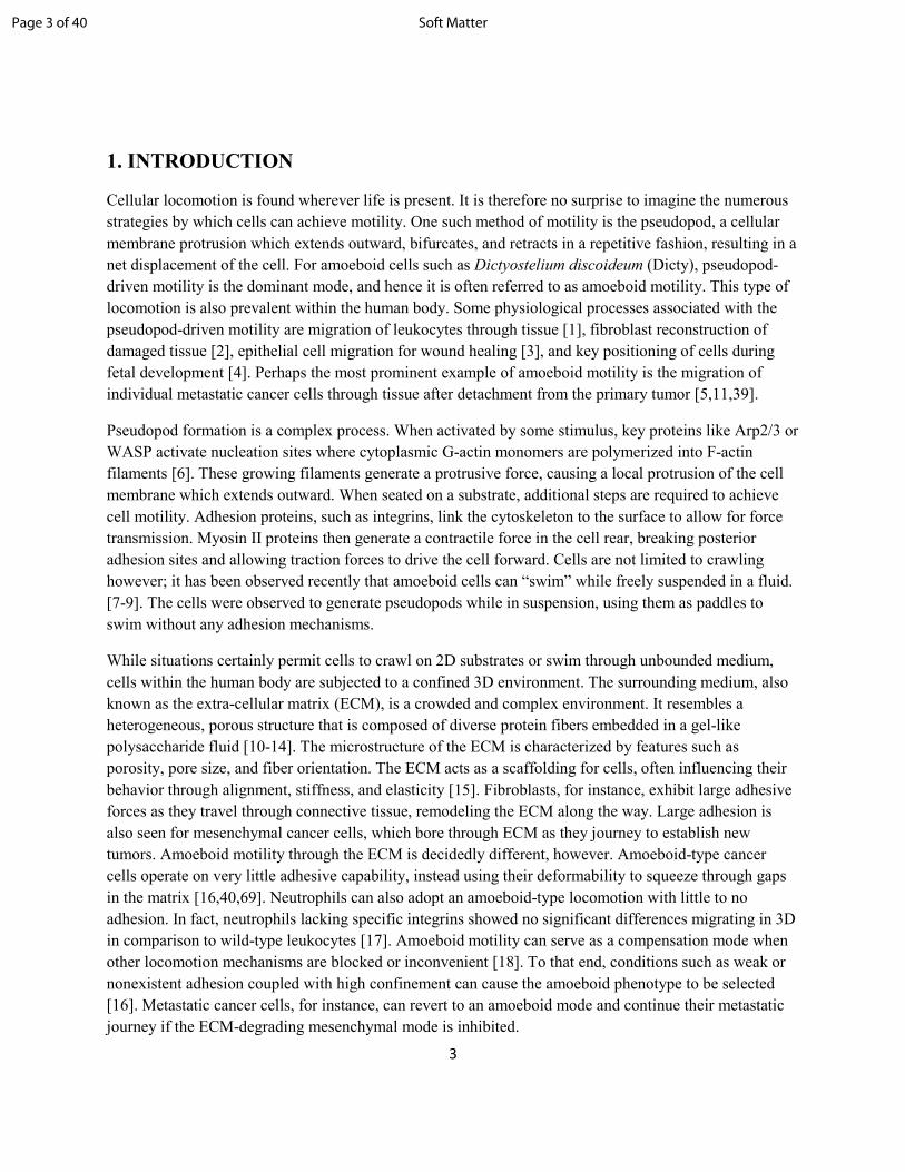
Cellular locomotion is found wherever life is present. It is therefore no surprise to imagine the numerous

strategies by which cells can achieve motility. One such method of motility is the pseudopod, a cellular

membrane protrusion which extends outward, bifurcates, and retracts in a repetitive fashion, resulting in a

net displacement of the cell. For amoeboid cells such as Dictyostelium discoideum (Dicty), pseudopod-

driven motility is the dominant mode, and hence it is often referred to as amoeboid motility. This type of

locomotion is also prevalent within the human body. Some physiological processes associated with the

pseudopod-driven motility are migration of leukocytes through tissue [1], fibroblast reconstruction of

damaged tissue [2], epithelial cell migration for wound healing [3], and key positioning of cells during

fetal development [4]. Perhaps the most prominent example of amoeboid motility is the migration of

individual metastatic cancer cells through tissue after detachment from the primary tumor [5,11,39].

Pseudopod formation is a complex process. When activated by some stimulus, key proteins like Arp2/3 or

WASP activate nucleation sites where cytoplasmic G-actin monomers are polymerized into F-actin

filaments [6]. These growing filaments generate a protrusive force, causing a local protrusion of the cell

membrane which extends outward. When seated on a substrate, additional steps are required to achieve

cell motility. Adhesion proteins, such as integrins, link the cytoskeleton to the surface to allow for force

transmission. Myosin II proteins then generate a contractile force in the cell rear, breaking posterior

adhesion sites and allowing traction forces to drive the cell forward. Cells are not limited to crawling

however; it has been observed recently that amoeboid cells can “swim” while freely suspended in a fluid.

[7-9]. The cells were observed to generate pseudopods while in suspension, using them as paddles to

swim without any adhesion mechanisms.

While situations certainly permit cells to crawl on 2D substrates or swim through unbounded medium,

cells within the human body are subjected to a confined 3D environment. The surrounding medium, also

known as the extra-cellular matrix (ECM), is a crowded and complex environment. It resembles a

heterogeneous, porous structure that is composed of diverse protein fibers embedded in a gel-like

polysaccharide fluid [10-14]. The microstructure of the ECM is characterized by features such as

porosity, pore size, and fiber orientation. The ECM acts as a scaffolding for cells, often influencing their

behavior through alignment, stiffness, and elasticity [15]. Fibroblasts, for instance, exhibit large adhesive

forces as they travel through connective tissue, remodeling the ECM along the way. Large adhesion is

also seen for mesenchymal cancer cells, which bore through ECM as they journey to establish new

tumors. Amoeboid motility through the ECM is decidedly different, however. Amoeboid-type cancer

cells operate on very little adhesive capability, instead using their deformability to squeeze through gaps

in the matrix [16,40,69]. Neutrophils can also adopt an amoeboid-type locomotion with little to no

adhesion. In fact, neutrophils lacking specific integrins showed no significant differences migrating in 3D

in comparison to wild-type leukocytes [17]. Amoeboid motility can serve as a compensation mode when

other locomotion mechanisms are blocked or inconvenient [18]. To that end, conditions such as weak or

nonexistent adhesion coupled with high confinement can cause the amoeboid phenotype to be selected

[16]. Metastatic cancer cells, for instance, can revert to an amoeboid mode and continue their metastatic

journey if the ECM-degrading mesenchymal mode is inhibited.


4

The objective of this current work is to present a computational modeling study of amoeboid motility in

confined medium. A number of previous studies have investigated cell motility in confined space using

numerical modeling approaches. Wu et al modeled the adhesion-free swimming of a 2D amoeboid cell

through a confined microchannel using the boundary integral method and force harmonics to represent the

active protrusive and contractile forces [19]. They found that sufficient confinement induces a maximum

swimming speed before reducing in magnitude. Lim et al developed a 2D model of bleb-based, adhesion-

free migration of amoeboid cells through microchannels of increasing confinement. The cell was modeled

by an elastic actin cortex surrounded by an elastic membrane connected by Hookean adhesion, and the

boundary integral method was used [20]. They showed migration was possible in the absence of substrate

adhesion, and that to a certain limit, increasing confinement in a microchannel increased migration speed.

Schlüter et al examined the dynamics of a 2D rigid adhesive cell migrating on a 2D substrate composed

of movable cylindrical fibers using Stoke’s drag, while considering matrix stiffness and orientation [21].

Results showed cells preferred stiffer matrices over softer ones, and cell persistence increased with fiber

orientation. Elliott et al simulated both 2D and 3D motility using an activator-inhibitor system coupled

with an evolving surface finite element method, and predicted bifurcating pseudopods [22]. They

considered 3D unbounded medium, and 2D porous medium represented by rigid but moveable spherical

obstacles. Intra- and extra-cellular fluids were not considered, and adhesion was modeled as a frictional

force. Hecht et al simulated a crawling 2D adhesion-free amoeboid cell exposed to a chemotactic gradient

in unbounded flow, and in the presence of obstacles and maze geometries [23]. Moure and Gomez

developed a phase-field model for a 3D amoeboid cell, including an activator-inhibitor system to describe

the cell biochemistry, transport equations to describe cytosolic biochemistry dynamics, and hydrodynamic

drag to describe adhesive forces [24]. Simulations were performed in 2D for cells navigating around

obstacles on a substrate, and in 3D for cells in rigid periodic cylindrical fibrous networks.

Apart from the aforementioned studies that considered motility in confined medium, there exists many

noteworthy studies that have modeled general amoeboid motility. For example, Vanderlei et al. [25]

developed a 2D model of motile cells using an immersed-boundary method that resolves cell deformation,

internal and external fluid flow, and a reaction-diffusion system in the entire volume of the cell. Bottino

and Fauci [26] developed a 2D model also using an immersed-boundary method in which the

cytoskeleton is represented as a dynamic network of springs immersed in a fluid. Their model was able to

generate protrusive and contractile forces as well as the attachment-detachment cycle in a cell crawling

over a substrate. Farutin et al. [27] considered a deformable cell driven under a prescribed axisymmetric

oscillating force in an unbounded medium. Najem & Grant [28] used a phase field approach to simulate

migration of neutrophils in 3D in response to external cues, but neglected the presence of fluids.

While significant advancement has been achieved in modeling amoeboid motility, a full 3D modeling in a

confined medium remains a challenge. Modeling cell migration in 3D environments is important, because

as noted above, ECM confinement which is known to heavily influence cell migration cannot be

replicated fully in 2D [12]. Additionally, numerical simulation allows us to independently vary important

cell and matrix parameters which may not be possible in experiments. Towards that end, in this article we

present a 3D modeling of pseudopod-driven amoeboid cell motility through a porous extracellular

medium. The extracellular space is made of a viscous fluid surrounding an array of finite-size, rigid, non-

moving spheres. Our model combines activator/inhibitor reaction/diffusion, extreme deformation of the

cell, pseudopod dynamics, cytoplasmic and extracellular fluid motion, and a fully resolved extracellular


5

environment. The methodology is based on the immersed-boundary method which allows a seamless

integration of diverse types of interfaces, both deformable and rigid. Our model predicts highly complex

and dynamically changing cell shapes similar to those observed in experiments with amoeba. Simulation

results are presented on the effects of matrix porosity, cell deformability, and obstacle to cell size ratio.

The Influence of confinement on motility behavior and some novel obstacle-mediated dynamics are

presented. It is shown that cells lack motile persistence in confined medium, and cell motion can be

completely hindered below certain values of matrix porosity, cell deformability, and obstacle size.

Comparisons are made of motility behaviors in confined and fully-unconfined medium, and the

differences are explained in terms of pseudopod dynamics.

2. MODEL

A multiscale, multiphysics computational model coupling fluid mechanics, solid mechanics, and pattern

formation is developed to simulate fully 3D, pseudopod-driven motility of amoeboid cells through a fluid

filled porous medium. The extra-cellular porous space is composed of an extracellular fluid and a regular

lattice of finite-size, rigid, non-moving spherical obstacles (figures 1 and 2). An amoeboid cell in our

model moves through the fluid-filled gaps between the obstacles. Although this simplified model of the

extra-cellular space does not exactly represent the complex ECM microenvironment, it allows for a

detailed parametric study in terms of the effect of ECM porosity and obstacle size. Along with this simple

ECM geometry, the model integrates actin-based pseudopod-dynamics, cell deformation, and intra- and

extra-cellular fluid motion. Our current model does not include cell-matrix adhesion. While adhesion

plays an important role in various forms of motility, amoeboid motility can occur with nearly no adhesion

as noted in §1. In addition to the aforementioned examples, adhesion-free “swimming”-type motility has

been recently observed in diverse scenario, e.g., for fat body cells and progenitor cells [67,68]; see also

Ref. [69]. Different components of the model and their numerical solution techniques are discussed

below. The models dealing with cell deformation have been described in several of our prior studies [29-

31], while the pseudopod generator model is described in [32]. Nevertheless, we briefly discuss these

modeling components for the sake of completeness. The specific new contribution in terms of numerical

technique is the consideration of the ECM.

2.1 Model of deformable cells

Cell deformability is an inherent requirement for pseudopod dynamics, and hence for amoeboid motility.

Deformation allows cells to create, divide, and retract pseudopods. The pseudopod dynamics, in turn,

result in highly complex and continuously changing cell shapes [6-9,33,34,38]. Protrusive forces from

growing actin filaments deform the cell membrane to generate pseudopods. The cell membrane has a

composite structure that is made of a lipid bilayer and an underlying cortex, with a combined thickness

that is orders of magnitude less compared to the size of the entire cell. [57]. On the scale of the whole

cell, the molecular details of the membrane can be coarse-grained as a zero-thickness (i.e. 2D)

hyperelastic sheet. On the same account, the interior of the cell, which contains the cytoplasm and a very

complex mixture of diverse proteins, is also modeled as a viscous liquid. Though molecular details are

neglected, this model still allows for force-mediated extreme deformation of the cell whose numerical

evaluation in 3D could be a complex problem depending on the physical laws assumed to govern the

membrane and intracellular fluid properties. In our continuum representation, the stresses generated in the

R1, #1


6

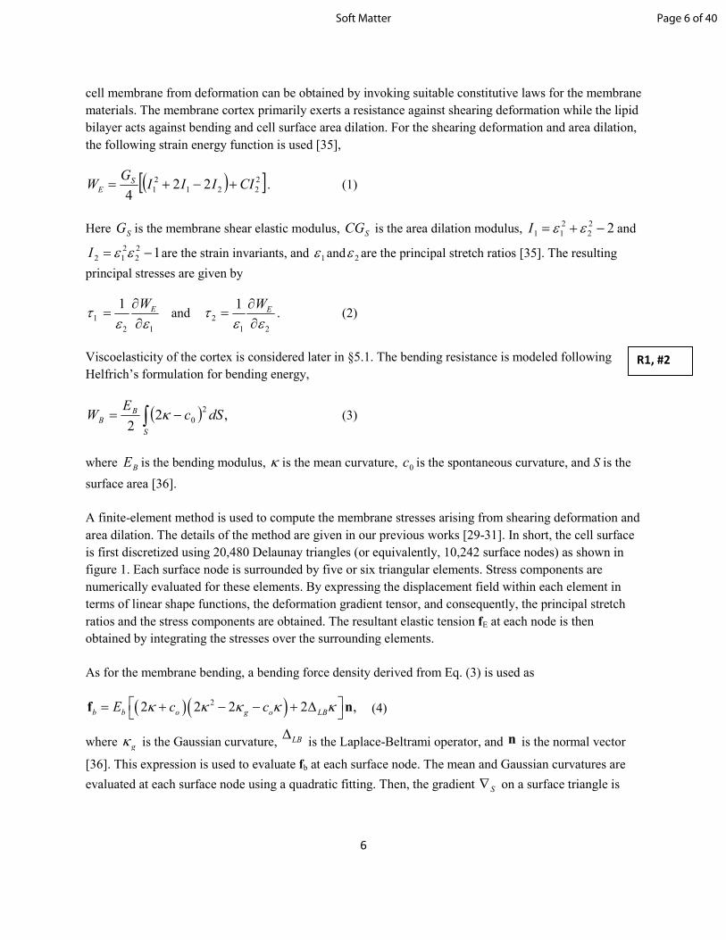
cell membrane from deformation can be obtained by invoking suitable constitutive laws for the membrane

materials. The membrane cortex primarily exerts a resistance against shearing deformation while the lipid

bilayer acts against bending and cell surface area dilation. For the shearing deformation and area dilation,

the following strain energy function is used [35],

( )[ ]2

221

2

1 224

CIIIIG

W SE +−+= . (1)

Here SG is the membrane shear elastic modulus, SCG is the area dilation modulus, 22

2

2

11 −+= εεI and

12

2

2

12 −= εεI are the strain invariants, and 1ε and 2ε are the principal stretch ratios [35]. The resulting

principal stresses are given by

12

1

1

εετ

∂∂

= EW and

21

2

1

εετ

∂∂

= EW. (2)

Viscoelasticity of the cortex is considered later in §5.1. The bending resistance is modeled following

Helfrich’s formulation for bending energy,

( )∫ −=S

BB dSc

EW ,2

2

2

0κ (3)

where BE is the bending modulus, κ is the mean curvature, 0c is the spontaneous curvature, and S is the

surface area [36].

A finite-element method is used to compute the membrane stresses arising from shearing deformation and

area dilation. The details of the method are given in our previous works [29-31]. In short, the cell surface

is first discretized using 20,480 Delaunay triangles (or equivalently, 10,242 surface nodes) as shown in

figure 1. Each surface node is surrounded by five or six triangular elements. Stress components are

numerically evaluated for these elements. By expressing the displacement field within each element in

terms of linear shape functions, the deformation gradient tensor, and consequently, the principal stretch

ratios and the stress components are obtained. The resultant elastic tension fE at each node is then

obtained by integrating the stresses over the surrounding elements.

As for the membrane bending, a bending force density derived from Eq. (3) is used as

( )( )22 2 2 2 ,b b o g o LBE c cκ κ κ κ κ = + − − + ∆ f n (4)

where gκ is the Gaussian curvature, LB∆ is the Laplace-Beltrami operator, and n is the normal vector

[36]. This expression is used to evaluate fb at each surface node. The mean and Gaussian curvatures are

evaluated at each surface node using a quadratic fitting. Then, the gradient S∇ on a surface triangle is

R1, #2


7

obtained by a linear interpolation of the surface and κ , and LBκ∆ is approximated using the Gauss

theorem. Additional details of this computation are given in Ref. [30].

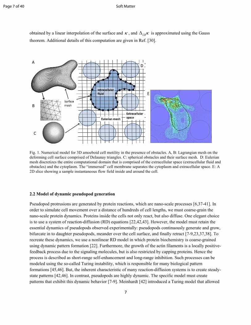
Fig. 1. Numerical model for 3D amoeboid cell motility in the presence of obstacles. A, B: Lagrangian mesh on the

deforming cell surface comprised of Delaunay triangles. C: spherical obstacles and their surface mesh. D: Eulerian

mesh discretizes the entire computational domain that is comprised of the extracellular space (extracellular fluid and

obstacles) and the cytoplasm. The “immersed” cell membrane separates the cytoplasm and extracellular space. E: A

2D slice showing a sample instantaneous flow field inside and around the cell.

2.2 Model of dynamic pseudopod generation

Pseudopod protrusions are generated by protein reactions, which are nano-scale processes [6,37-41]. In

order to simulate cell movement over a distance of hundreds of cell lengths, we must coarse-grain the

nano-scale protein dynamics. Proteins inside the cells not only react, but also diffuse. One elegant choice

is to use a system of reaction-diffusion (RD) equations [22,42,43]. However, the model must retain the

essential dynamics of pseudopods observed experimentally: pseudopods continuously generate and grow,

bifurcate in to daughter pseudopods, meander over the cell surface, and finally retract [7-9,23,37,38]. To

recreate these dynamics, we use a nonlinear RD model in which protein biochemistry is coarse-grained

using dynamic pattern formation [22]. Furthermore, the growth of the actin filaments is a locally positive-

feedback process due to the signaling molecules, but is also restricted by capping proteins. Hence the

process is described as short-range self-enhancement and long-range inhibition. Such processes can be

modeled using the so-called Turing instability, which is responsible for many biological pattern

formations [45,46]. But, the inherent characteristic of many reaction-diffusion systems is to create steady-

state patterns [42,46]. In contrast, pseudopods are highly dynamic. The specific model must create

patterns that exhibit this dynamic behavior [7-9]. Meinhardt [42] introduced a Turing model that allowed


8

for dynamic pattern formation suitable for pseudopod generation [22,43,47]. This model utilizes the

behavior of several competing species which are called activators and inhibitors. The activators can be

thought to represent nucleating proteins and actin filaments, while the inhibitors could represent filament

capping and severing proteins. By varying the diffusion rates of the species, dynamic patterns can be

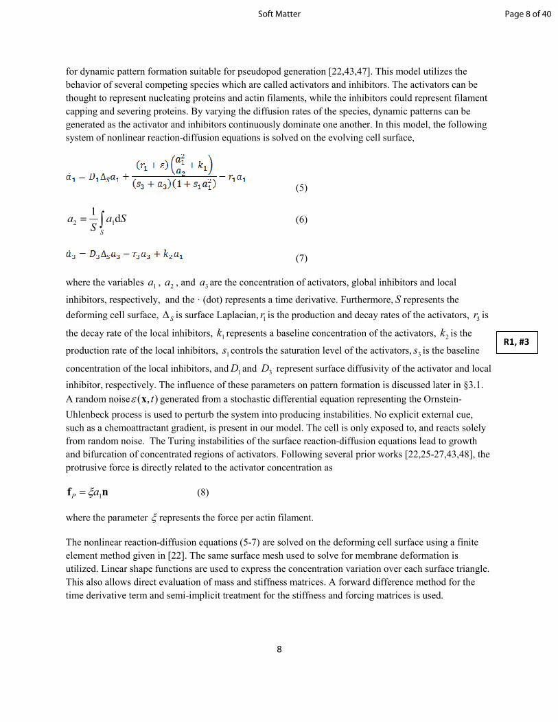
generated as the activator and inhibitors continuously dominate one another. In this model, the following

system of nonlinear reaction-diffusion equations is solved on the evolving cell surface,

(5)

∫=S

SaS

a d1

12 (6)

(7)

where the variables 1a , 2a , and 3a are the concentration of activators, global inhibitors and local

inhibitors, respectively, and the · (dot) represents a time derivative. Furthermore, S represents the

deforming cell surface, S∆ is surface Laplacian, 1r is the production and decay rates of the activators, 3r is

the decay rate of the local inhibitors, 1k represents a baseline concentration of the activators, 2k is the

production rate of the local inhibitors, 1s controls the saturation level of the activators, 3s is the baseline

concentration of the local inhibitors, and 1D and 3D represent surface diffusivity of the activator and local

inhibitor, respectively. The influence of these parameters on pattern formation is discussed later in §3.1.

A random noise ),( txε generated from a stochastic differential equation representing the Ornstein-

Uhlenbeck process is used to perturb the system into producing instabilities. No explicit external cue,

such as a chemoattractant gradient, is present in our model. The cell is only exposed to, and reacts solely

from random noise. The Turing instabilities of the surface reaction-diffusion equations lead to growth

and bifurcation of concentrated regions of activators. Following several prior works [22,25-27,43,48], the

protrusive force is directly related to the activator concentration as

nf 1aP ξ= (8)

where the parameter ξ represents the force per actin filament.

The nonlinear reaction-diffusion equations (5-7) are solved on the deforming cell surface using a finite

element method given in [22]. The same surface mesh used to solve for membrane deformation is

utilized. Linear shape functions are used to express the concentration variation over each surface triangle.

This also allows direct evaluation of mass and stiffness matrices. A forward difference method for the

time derivative term and semi-implicit treatment for the stiffness and forcing matrices is used.

R1, #3


9

2.3 Cytoplasmic and extra-cellular fluids

The cytoplasm and extracellular fluid are assumed to be incompressible and Newtonian. Since inertia is

negligible, the fluid motion is governed by the Stokes equations and the incompressibility condition.

[ ]T0 uu ∇+∇⋅∇+−∇= µp (9)

0=⋅∇ u (10)

where u and p

represent the fluid velocity and pressure fields both in the cytoplasm and in the

extracellular fluid. We assume that the densities and viscosities of the cytoplasmic and extracellular fluids

are same and equal to those of water. This assumption is not a limitation of the methodology; the

influence of viscosity difference between the two fluids has been considered in our previous work [32].

We further assume that the extracellular fluid is otherwise stagnant; however, movement of the cell

causes the fluid to displace.

The cell membrane is “immersed” within the surrounding fluid. The coupling between the protrusive

force, membrane deformation, and fluid motion in the cytoplasm and extracellular fluid is done using the

continuous forcing immersed-boundary method (IBM) [49]. It is an efficient way of dealing with

problems involving highly complex and deformable interfaces without using a body conforming mesh. In

this approach, a single set of governing equations is written for both the interior and exterior of the cell,

while an indicator function is used to differentiate between the two zones. The presence of the membrane,

which is the interface between the two fluids, is accounted for by introducing a source term in the Stokes

equation which includes the forces acting on the cell membrane as

[ ] ( )∫ +++∇+∇⋅∇+−∇=S

PBE Sp d 0 T δµ fffuu (11)

where δ is the 3D Dirac delta function, S represents the cell surface, fE and fB are the membrane forces

arising from shearing deformation and area dilation, and bending, respectively, and fP is the protrusive

force. The delta function is zero everywhere except at the location of the membrane, and is used to couple

the protrusive and membrane forces to the fluid motion. The delta function is numerically approximated

with a cosine function spanning over four Eulerian points around the cell boundary as

( ) ( )∏=

′−∆

+∆

=′−3

13 2

cos164

1

i

ii xxxxπ

δ , for ∆≤′− 2ii xx , 3,2,1=i

0= , otherwise, (12)

where ∆ is the size of a computational mesh in the fluid domain, ix is a fluid node, and ix′ is a

Lagrangian node on the cell surface [50].

Once the fluid velocity is obtained by solving Eq. (11), the membrane velocity mu is computed by

interpolating the fluid velocity from the surrounding Eulerian nodes using the Delta function as


10

( ) ( ) xxxxuxu dS

m )( ′−=′ ∫ δ . (13)

Then, the membrane nodes mx are advected as mm t ux =d/d , resulting in a new location and deformed

shape of the cell. It may be noted that the above method directly couples the fluid motion with the

membrane deformation. Thus, the effect of fluid drag on cell movement is directly resolved. No ad hoc

modeling of fluid drag is needed here unlike some earlier works [22,47,51-54].

The computational domain includes the cell and its membrane, intra- and extra-cellular fluids, and

obstacles. It is a cubic domain with lengths about 19 times the cell radius for most simulations. The

domain is discretized using a fixed (Eulerian) rectangular mesh of 3603 nodes (figure 1). The governing

equations for fluid motion are solved on this mesh. The numerical technique is given in detail in [55], and

is briefly discussed here. We use a projection method for time integration of the unsteady Stokes

equations. The projection method is usually used for the full Navier-Stokes equations, but is considered

here more suitable for the IBM implementation. In this approach, an advection-diffusion equation is first

solved, followed by a Poisson-type equation to enforce the incompressibility condition. In the first step,

the body force terms representing the membrane and protrusive forces are treated explicitly using a

second-order Adams-Bashforth scheme, and the viscous terms are treated semi-implicitly using the

Crank-Nicholson scheme. A staggered arrangement for the variables in the Eulerian mesh is used by

defining the velocity components at the edges of an Eulerian mesh element, and pressure at the element

center. All spatial derivatives are evaluated using second-order differencing. The advection-diffusion

equation is solved using an alternating direction implicit (ADI) scheme which allows for fast inversion of

matrices and a robust technique when complex boundaries are involved. The Poisson equation must be

solved implicitly to satisfy the incompressibility condition. The periodicity of the computational domain

allows us to use the Fourier expansion, and hence a fast, implicit solution.

2.4 Modeling extracellular objects

As mentioned before, the extracellular objects are modeled as rigid, non-moving spheres of finite size that

are “immersed” within the extracellular fluid, and therefore, within the Eulerian mesh (figure 1). These

obstacles define the “solid phase”, and together with the extracellular fluid, they constitute the porous,

extra-cellular space. The fluid must satisfy the no-slip condition on the surface of the obstacles. The

continuous forcing IBM that is suitable for elastic interfaces as discussed in §2.3, however, is not well-

behaved for rigid boundaries for which we use a direct forcing IBM, namely the sharp-interface Ghost-

Node method (GNIBM). The GNIBM method has been implemented in our previous publication in the

context of deformable blood cells flowing through highly complex geometry [55]. The general

methodology can be applied to treat rigid objects of any arbitrary shape, and not just spherical objects as

considered in the present study. The basic premise of the method is how to enforce the no-slip condition

along a rigid surface that does not coincide with the rectangular Eulerian mesh. Such a condition is

achieved in the GNIBM by enforcing a constraint at certain Eulerian grid points. In this approach, first the

surface of each spherical obstacle is discretized using 1280 Delaunay triangles (or, 642 nodes). The

Eulerian nodes residing inside the spheres that are immediately next to the sphere surface are labeled as

ghost nodes (GN). The intercept of the sphere surface and the surface normal passing through a ghost

node is labeled as a boundary intercept (BI). A point outside the sphere that lies along this normal but as


11

equidistant from the BI as the GN is labeled as image point (IP). The velocity uBI at the BI is taken as the

average of the values at the GN and IP, that is, (uGN + uIP)/2. By letting uBI = 0 to satisfy the no-slip

condition, the condition at a GN is obtained as uGN = ―uIP, which is enforced while solving the governing

equations for fluid flow. A trilinear interpolation is used to obtain uIP from the surrounding Eulerian

nodes.

2.5 Model parameters and validation

The initial undeformed shape of the cell is assumed to be spherical. The simulation results are presented

using dimensionless variables. Lengths are scaled by the cell radius R , time is scaled by 1

2 / DR , and

velocities are scaled by RD /1 , where D1 is the activator diffusivity. The spherical obstacles are arranged

in a regular lattice (figure 2). The major dimensionless parameters defining the extracellular space are the

porosity (void fraction) ϕ, defined as the ratio of the extracellular fluid volume to total volume, and the

ratio of the radius of each obstacle to that of the cell γ = RO /R. The parameter that defines the cell

deformability is the ratio of the protrusive force to membrane elastic force SRG/ξα = . Finally, the

major parameter of interest in the reaction-diffusion model is the ratio of inhibitor to activator

diffusivities 13 / DD=β . The force per actin filament is in the range 3—8 pN [56], cell radius ~R 10

µm [37], 1D and ~3D 1 µm2/s [56], and membrane shear modulus ~SG 10

―6 N/m [57]. Membrane

stiffness varies in cells. For instance, immune cells are relatively softer than fibroblasts [2]. Stiffness also

varies in malignant and drug-treated cells [58-61]. Our interest in the present work is in the role of matrix

porosity ϕ, obstacle size ratio γ, and cell deformability as defined by α. Matrix porosity is varied from

0.54 to 1, representing highly confined to fully unbounded medium. This range corresponds to

physiological conditions in addition to those encountered in tissue engineering [70]. Connective tissue,

for example, is characterized by loose fibers, while the basal laminae is composed of densely-packed

crosslinked tissue. The range of γ, determined from numerical experiments, is 0.25 to 2: The lower bound

is usually reached when cell motion is completely hindered due to confinement, while the upper bound

can represent interstitial blood vessels or impassable geometries. The suitable ranges of α and β have been

discussed in our prior work [32], and are selected such that experimentally observed bifurcating

pseudopod dynamics can be recreated in the model. Following this, we consider membrane deformability

in the range α = 1-7 and β = 3 in the present work. Additional parameters in the RD equations are also

listed in [32] and kept constants in the present study.

Extensive validation of the cell deformation model has been done in our previous works [29,30,55]. This

includes numerical experiments of cell aspiration in a micropipette, and cell deformation in externally

applied shear flow. For brevity, we avoid repeating these studies here. Validation of the reaction-diffusion

model was presented in [32]. There it was shown that our model can accurately predict various types of

Turing instabilities on curved surfaces. A detailed study of pseudopod-driven motility in unconfined

medium was also presented there. It was shown that the predicted cell shapes were qualitatively similar to

those observed in experiments [7-9,37,44]. Predicted cell speeds also agreed very well with

experimentally measured cell speeds. Instantaneous fluid velocity vectors both inside and outside the cell

from one current simulation are presented in figure 1E, which shows the complexity of the flow field

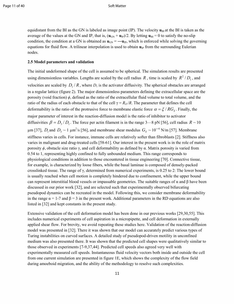
during amoeboid migration, and the ability of the methodology to resolve such complexities.


12

Cell volume is preserved within about 1% (see figure S5 in Supplementary Materials). No explicit

volume preserving force is used. This may be due to the use of very high resolution on the cell surface,

and accuracy in satisfying the incompressibility condition.

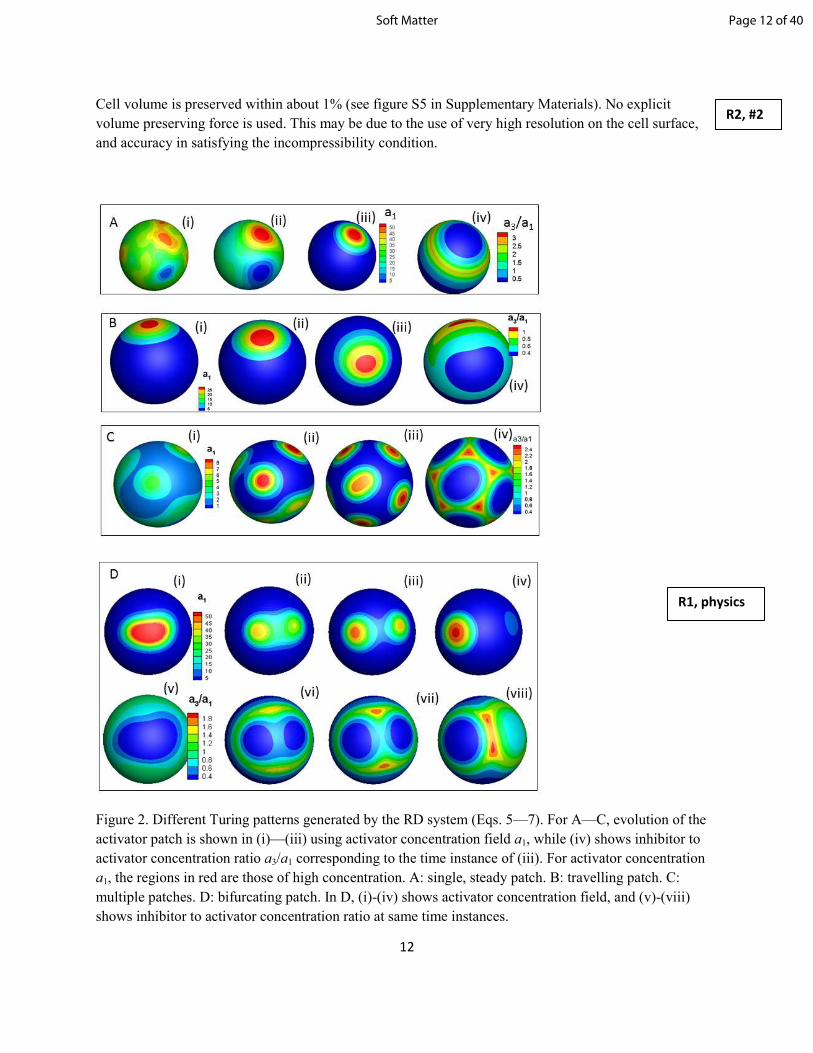
Figure 2. Different Turing patterns generated by the RD system (Eqs. 5—7). For A—C, evolution of the

activator patch is shown in (i)—(iii) using activator concentration field a1, while (iv) shows inhibitor to

activator concentration ratio a3/a1 corresponding to the time instance of (iii). For activator concentration

a1, the regions in red are those of high concentration. A: single, steady patch. B: travelling patch. C:

multiple patches. D: bifurcating patch. In D, (i)-(iv) shows activator concentration field, and (v)-(viii)

shows inhibitor to activator concentration ratio at same time instances.

R2, #2

R1, physics


13

3. Interaction between reaction-diffusion, surface shape, and deformation

Before presenting the results on cell motility, we present insights on interaction between the RD system,

surface shape, and deformation. First, in §3.1 we consider the Turing patterns on the surface of a rigid

sphere. Then, in §3.2 we consider the influence of surface curvature. The influence of a deforming surface

is explained in §3.3. Finally, the presence of obstacles is considered in §3.4. These physical insights help

to explain the pseudopod-driven motility presented in §4.

3.1 Turing patterns on rigid spheres

The Turing instabilities of the RD equations lead to growth and bifurcation of concentrated regions of

activators. The activator equation (Eq. 5) represents a positive-feedback (self-enhancing) process. A small

local increase in the activator concentration by the random noise ε is further enhanced due to the

nonlinear reaction term which depends on 2

2

1 / aa (see figure 2A). The growth of the activator is also

accompanied by an increase in inhibitors (both and ) concentration via Eqs. 6-7. The global

inhibitor , via Eq. 6, overpowers and annihilates the activator everywhere except at incipient site where

both a1 and a3 continue to grow creating localized region(s) of high concentration. As both activator and

local inhibitor concentrations grow, increased gradient also causes increased diffusion away from this

site. Eventually a dynamic equilibrium is established under the balance of production, annihilation, and

diffusion leading to a specific pattern of localized regions of high activator concentration. This process is

shown using an example simulation in figure 2A(i)-(iii) demonstrating the growth of a single, steady

activator patch by a random noise. Figure 2A(iv) shows the ratio a3/a1 at steady state, which suggests that

the activator patch is surrounded by a ring of higher inhibitor concentration; thus, the instability is

essentially in equilibrium, as any attempt to diffuse away is met by activator depletion.

Different patterns can be generated by varying the parameters in the RD equations, for instance, a single,

but travelling patch as in figure 2B, multiple steady patches as in figure 2C, and a bifurcating pattern as in

figure 2D. The single or multiple, steady patches are generated when inhibitor diffusion is faster than

activator diffusion (D3 > D1). A travelling patch is formed when their diffusion is comparable (D3/D1 ~1).

In all these patterns, the region of high activator concentration is surrounded by a ring of high a3/a1,

which dictates the nature of the dynamic equilibrium. For instance, for the travelling patch, the ring has a

non-uniform thickness. Because of this, activator diffusing towards the thick end is quickly annihilated by

the inhibitor, while activator diffusing towards the thin end is virtually unaffected, allowing it to meander

over the sphere surface.

A bifurcating pattern is formed when activator reaction rate r1 is large. As shown in the figure, an

activator patch is generated, but because of large r1 it quickly bifurcates creating two daughter patches. A

wedge-shaped region of high a3/a1 is drawn between the two daughter patches. In time, one patch is

annihilated, and the remaining patch bifurcates again as the pattern repeats.

The phase diagrams for different patterns obtained on a rigid sphere by varying β = D3/D1, r1, and s1 are

given in the Supplementary Materials (figure S1); it shows the sensitivity of the patterns to the

parameters. The pattern relevant for the pseudopod-based motility is the bifurcating pattern as it mimics

R1, #3

R1, Physics


14

bifurcating pseudopods. Thus, in subsequent analysis, we limit our parameter values to bifurcating

patterns only (see §2.5).

3.2 Influence of curvature on Turing patterns

The discussion above was for Turing patterns on a rigid sphere. We now consider the influence of surface

curvature. Previous works have shown that diffusion is dependent on surface curvature, and, species

concentrate on a convex surface (positive Gaussian curvature), but away from a hyperbolic surface

(negative Gaussian curvature) [71,72].The former mechanism causes a faster growth of activator and

local inhibitor in the high curvature regions, and enhances the instability of Turing patterns. To show this,

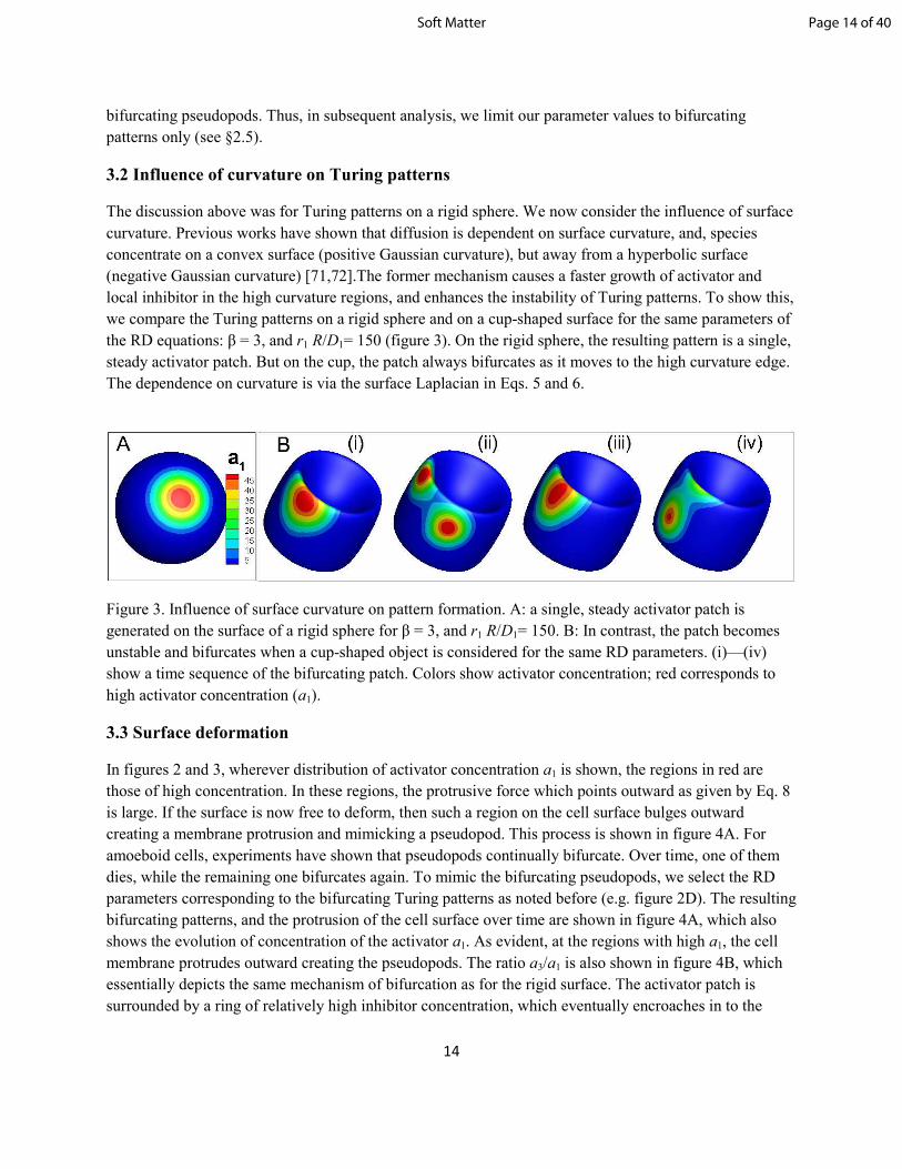
we compare the Turing patterns on a rigid sphere and on a cup-shaped surface for the same parameters of

the RD equations: β = 3, and r1 R/D1= 150 (figure 3). On the rigid sphere, the resulting pattern is a single,

steady activator patch. But on the cup, the patch always bifurcates as it moves to the high curvature edge.

The dependence on curvature is via the surface Laplacian in Eqs. 5 and 6.

Figure 3. Influence of surface curvature on pattern formation. A: a single, steady activator patch is

generated on the surface of a rigid sphere for β = 3, and r1 R/D1= 150. B: In contrast, the patch becomes

unstable and bifurcates when a cup-shaped object is considered for the same RD parameters. (i)—(iv)

show a time sequence of the bifurcating patch. Colors show activator concentration; red corresponds to

high activator concentration (a1).

3.3 Surface deformation

In figures 2 and 3, wherever distribution of activator concentration a1 is shown, the regions in red are

those of high concentration. In these regions, the protrusive force which points outward as given by Eq. 8

is large. If the surface is now free to deform, then such a region on the cell surface bulges outward

creating a membrane protrusion and mimicking a pseudopod. This process is shown in figure 4A. For

amoeboid cells, experiments have shown that pseudopods continually bifurcate. Over time, one of them

dies, while the remaining one bifurcates again. To mimic the bifurcating pseudopods, we select the RD

parameters corresponding to the bifurcating Turing patterns as noted before (e.g. figure 2D). The resulting

bifurcating patterns, and the protrusion of the cell surface over time are shown in figure 4A, which also

shows the evolution of concentration of the activator a1. As evident, at the regions with high a1, the cell

membrane protrudes outward creating the pseudopods. The ratio a3/a1 is also shown in figure 4B, which

essentially depicts the same mechanism of bifurcation as for the rigid surface. The activator patch is

surrounded by a ring of relatively high inhibitor concentration, which eventually encroaches in to the


15

activator patch causing it to bifurcate. Over a longer time, one of the daughter patches, and hence one of

the pseudopods, dies, while the other bifurcates repeating the cycle.

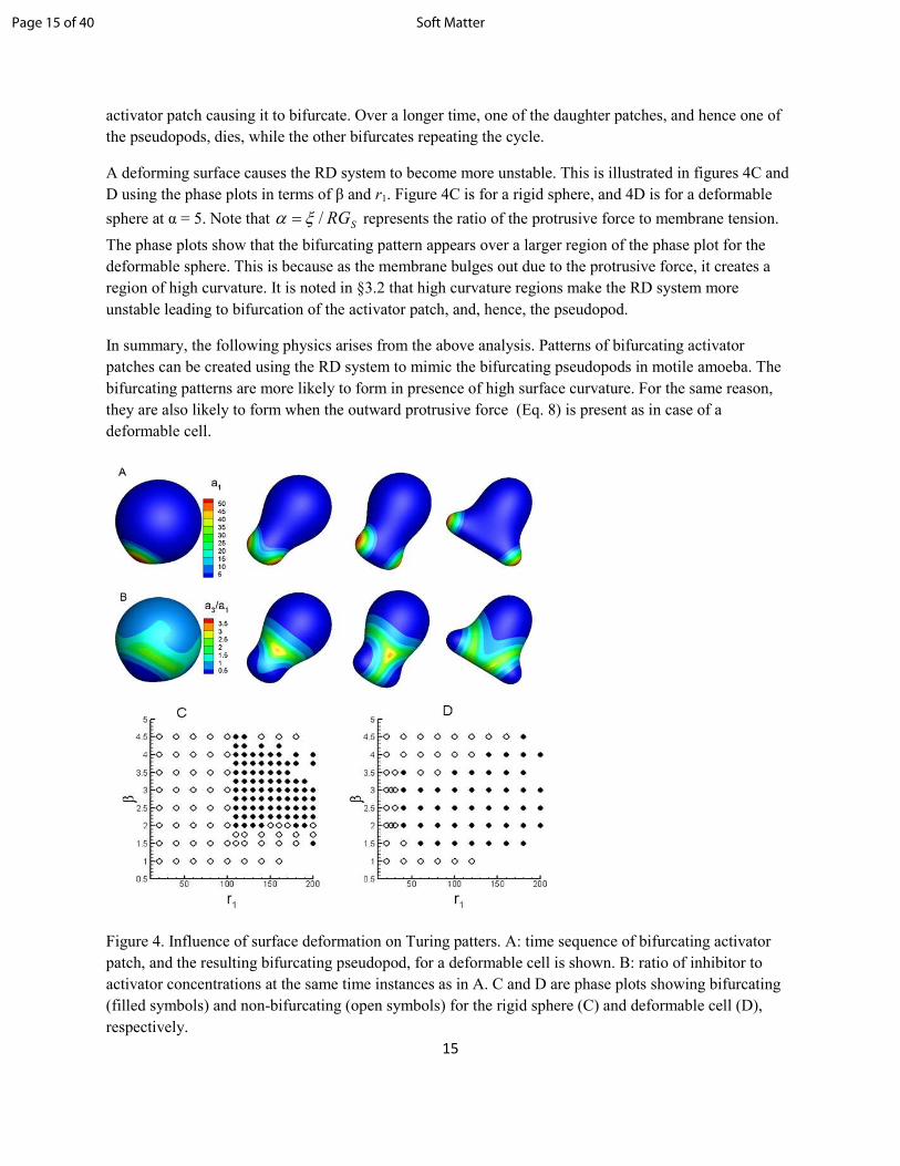
A deforming surface causes the RD system to become more unstable. This is illustrated in figures 4C and

D using the phase plots in terms of β and r1. Figure 4C is for a rigid sphere, and 4D is for a deformable

sphere at α = 5. Note that SRG/ξα = represents the ratio of the protrusive force to membrane tension.

The phase plots show that the bifurcating pattern appears over a larger region of the phase plot for the

deformable sphere. This is because as the membrane bulges out due to the protrusive force, it creates a

region of high curvature. It is noted in §3.2 that high curvature regions make the RD system more

unstable leading to bifurcation of the activator patch, and, hence, the pseudopod.

In summary, the following physics arises from the above analysis. Patterns of bifurcating activator

patches can be created using the RD system to mimic the bifurcating pseudopods in motile amoeba. The

bifurcating patterns are more likely to form in presence of high surface curvature. For the same reason,

they are also likely to form when the outward protrusive force (Eq. 8) is present as in case of a

deformable cell.

Figure 4. Influence of surface deformation on Turing patters. A: time sequence of bifurcating activator

patch, and the resulting bifurcating pseudopod, for a deformable cell is shown. B: ratio of inhibitor to

activator concentrations at the same time instances as in A. C and D are phase plots showing bifurcating

(filled symbols) and non-bifurcating (open symbols) for the rigid sphere (C) and deformable cell (D),

respectively.


16

3.4 Presence of obstacles

Figure 5 describes what happens when an obstacle is encountered. Two pseudopods wrap around it,

creating a concave front. Over time, one activator patch dies while the other bifurcates. As noted above

(§3.2), the high curvature near the rim of the concavity makes the activator/inhibitor system more

unstable causing the patch to bifurcate. In contrast, locally hyperbolic regions exist just below the rim

which stabilize the patch [71,72]. If the activator patch attempts to move out of the concave region by

crossing over the rim, it causes further extension of the rim (and, hence, further increase in rim curvature)

around the obstacle due to the protrusive force that is generated at these locations, thereby further

increasing the concavity. Consequently, the patch remains bounded in the concave region just below the

rim. Shortly thereafter, the patch bifurcates due to its own instability (as discussed in §3.1), and the

process repeats itself.

Therefore, it is the interaction between cell deformation and the obstacle that causes confinement of the

activator patches within the concave region. We have verified by additional simulations that if the cell is

not allowed to deform further after it has developed a concave front around an obstacle, the activator

patch can indeed move out of the concave region, and a pseudopod can form elsewhere.

Figure 5. Time sequence of pseudopod dynamics in presence of an obstacle (sphere in grey). Activator

concentration is shown in color, with red being the maximum concentration. The membrane protrudes

outward at regions of high activator concentration. Starting with two activator patches (A and B, as

shown), one of them (B) dies over time, while the other (A) bifurcates in to two daughter patches, and

hence, two pseudopods (A1 and A2). Subsequently A1 dies, and the process repeats. The activator patch

favors hyperbolic regions (§3.2). As it tries to move over the rim, it causes even more elongation of the

rim, thereby confining itself within the concave front.

Next we present the main results of this study.

R1, #5


17

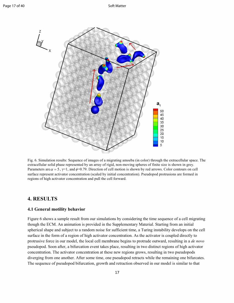
Fig. 6. Simulation results: Sequence of images of a migrating amoeba (in color) through the extracellular space. The

extracellular solid phase represented by an array of rigid, non-moving spheres of finite size is shown in grey.

Parameters are 5=α , γ=1, and ϕ=0.79. Direction of cell motion is shown by red arrows. Color contours on cell

surface represent activator concentration (scaled by initial concentration). Pseudopod protrusions are formed in

regions of high activator concentration and pull the cell forward.

4. RESULTS

4.1 General motility behavior

Figure 6 shows a sample result from our simulations by considering the time sequence of a cell migrating

though the ECM. An animation is provided in the Supplementary Material. Starting from an initial

spherical shape and subject to a random noise for sufficient time, a Turing instability develops on the cell

surface in the form of a region of high activator concentration. As the activator is coupled directly to

protrusive force in our model, the local cell membrane begins to protrude outward, resulting in a de novo

pseudopod. Soon after, a bifurcation event takes place, resulting in two distinct regions of high activator

concentration. The activator concentration at these new regions grows, resulting in two pseudopods

diverging from one another. After some time, one pseudopod retracts while the remaining one bifurcates.

The sequence of pseudopod bifurcation, growth and retraction observed in our model is similar to that


18

observed in experiments using crawling and swimming Dicty cells [7-9,34,37]. The cell squeezes through

the gaps as the resultant protrusive force acting on the pseudopods pulls it forward. The sequence in

figure 6 shows the cell is often highly deformed and confined as its pseudopods weave around and

through dense obstacles. Pseudopods are highly dynamic in nature, produced from leading-edge

bifurcations or by lateral de novo formation. The cell deforms because of the growing, bifurcating, and

retracting pseudopods, as well as its interaction with obstacles. The cell body often partly wraps around

an obstacle as the pseudopods at the front pull the cell. When obstacles preclude forward motion, the cell

is capable of turning back and retracing its path in order to find a more favorable direction. In addition,

the cell can send out two pseudopods in opposite directions, straddling around an obstacle. In time, one

pseudopod retracts, leaving the pseudopod free to pull the cell in its direction, thereby navigating around

the obstacle. These and several other mechanisms of navigation through obstacles are discussed later. As

noted in §3, the bifurcating Turing patterns mostly remain confined in regions of concavity near the cell

front.. Because of this, we must take necessary steps to ensure cells do not get stuck on obstacles. As a

first step to prevent a cell from directly hitting an obstacle surface, we add a lubrication pressure which

begins to act on the cell membrane when its distance from the obstacle is less than two Eulerian grid

points. Secondly, if an active pseudopod becomes closer than this distance, we terminate the

activator/inhibitor dynamics and reset their concentrations back to their initial value. This allows

generation of activator patches in new locations, and, hence, new pseudopods in alternate directions so

that the cell can continue its migration.

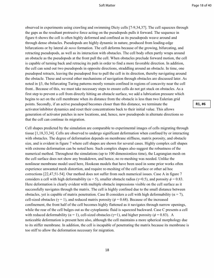
Cell shapes predicted by the simulation are comparable to experimental images of cells migrating through

tissue [1,18,33,34]. Cells are observed to undergo significant deformation when confined by or interacting

with obstacles. The degree of deformation depends on membrane stiffness, matrix porosity, and obstacle

size, and is evident in figure 7 where cell shapes are shown for several cases. Highly complex cell shapes

with extreme deformation can be noted here. Such complex shapes also suggest the robustness of the

numerical method. Throughout the simulations (up to 100 dimensionless time), the Lagrangian mesh on

the cell surface does not show any breakdown, and hence, no re-meshing was needed. Unlike the

nonlinear membrane model used here, Hookean models that have been used in some prior works often

experience unwanted mesh distortion, and require re-meshing of the cell surface or other ad hoc

corrections [22,47,51-54]. Our method does not suffer from such numerical issues. Case A in figure 7

considers a cell with high deformability (α = 5), smaller obstacle radius (γ=0.5), and porosity ϕ = 0.83.

Here deformation is clearly evident with multiple obstacle impressions visible on the cell surface as it

successfully navigates through the matrix. The cell is highly confined due to the small distance between

obstacles, yet is capable of matrix penetration. Case B considers a cell with high deformability (α = 7),

cell-sized obstacles (γ = 1), and reduced matrix porosity (ϕ = 0.68). Because of the increased

confinement, the front half of the cell becomes highly flattened as it navigates through narrow openings,

while the rear of the cell bulges out as the cytoplasmic fluid is squeezed backward. Case C presents a cell

with reduced deformability (α = 1), cell-sized obstacles (γ=1), and higher porosity (ϕ = 0.83). A

noticeable deformation is present here also, although the cell maintains a more spherical morphology due

to its stiffer membrane. In addition, the cell is incapable of penetrating the matrix because its membrane is

too stiff to allow the deformation necessary for migration.

R1, #6


19

Figure 7. Examples of highly complex cell shapes predicted by the simulations. A: α = 5, γ = 0.5, and ϕ = 0.83. B: α

= 7, γ = 1, and ϕ = 0.68. C: α = 1, γ = 1, and ϕ = 0.83.

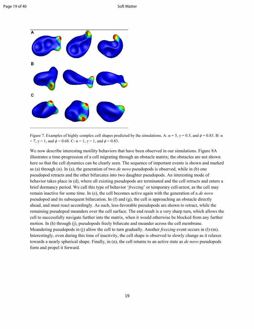
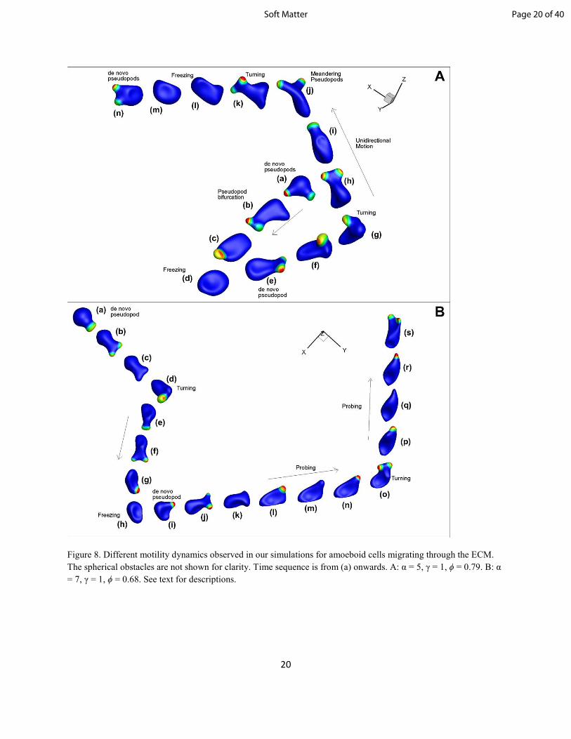
We now describe interesting motility behaviors that have been observed in our simulations. Figure 8A

illustrates a time-progression of a cell migrating through an obstacle matrix; the obstacles are not shown

here so that the cell dynamics can be clearly seen. The sequence of important events is shown and marked

as (a) through (n). In (a), the generation of two de novo pseudopods is observed, while in (b) one

pseudopod retracts and the other bifurcates into two daughter pseudopods. An interesting mode of

behavior takes place in (d), where all existing pseudopods are terminated and the cell retracts and enters a

brief dormancy period. We call this type of behavior ‘freezing’ or temporary cell-arrest, as the cell may

remain inactive for some time. In (e), the cell becomes active again with the generation of a de novo

pseudopod and its subsequent bifurcation. In (f) and (g), the cell is approaching an obstacle directly

ahead, and must react accordingly. As such, less-favorable pseudopods are shown to retract, while the

remaining pseudopod meanders over the cell surface. The end result is a very sharp turn, which allows the

cell to successfully navigate further into the matrix, when it would otherwise be blocked from any further

motion. In (h) through (j), pseudopods freely bifurcate and meander across the cell membrane.

Meandering pseudopods in (j) allow the cell to turn gradually. Another freezing event occurs in (l)-(m).

Interestingly, even during this time of inactivity, the cell shape is observed to slowly change as it relaxes

towards a nearly spherical shape. Finally, in (n), the cell returns to an active state as de novo pseudopods

form and propel it forward.


20

Figure 8. Different motility dynamics observed in our simulations for amoeboid cells migrating through the ECM.

The spherical obstacles are not shown for clarity. Time sequence is from (a) onwards. A: α = 5, γ = 1, ϕ = 0.79. B: α

= 7, γ = 1, ϕ = 0.68. See text for descriptions.


21

Figure 8B illustrates another interesting behavior predicted. Similar to the sequence in figure 8A, we have

a de novo pseudopod forming and bifurcating in (a)-(b). (c) shows pseudopod termination due to collision

with an obstacle, followed by a hard turn in (d). (e)-(g) show pseudopod bifurcation. In (h), a freezing

event occurs, causing the cell to retract and become inactive. In (i), the cell becomes active again with the

formation of a de novo pseudopod, which subsequently bifurcates in (j). In (l)-(n), the cell is restricted

within the same space while it sends out pseudopod protrusions, usually through narrow gaps in the

matrix, which are terminated after interacting with an obstacle. This happens repeatedly as the cell

manages to slowly overcome the obstacle with each new pseudopod. We refer to this behavior as probing

or groping. The difference between freezing and probing is that in the former, the pseudopods are

completely withdrawn and the cell becomes inactive for some time, while in the latter case, activator

concentration repeatedly grows and disappears resulting in cyclical phase of pseudopod extension and

pause. Additional probing events can be recognized in (p)-(s).

4.2 Obstacle-mediated dynamics

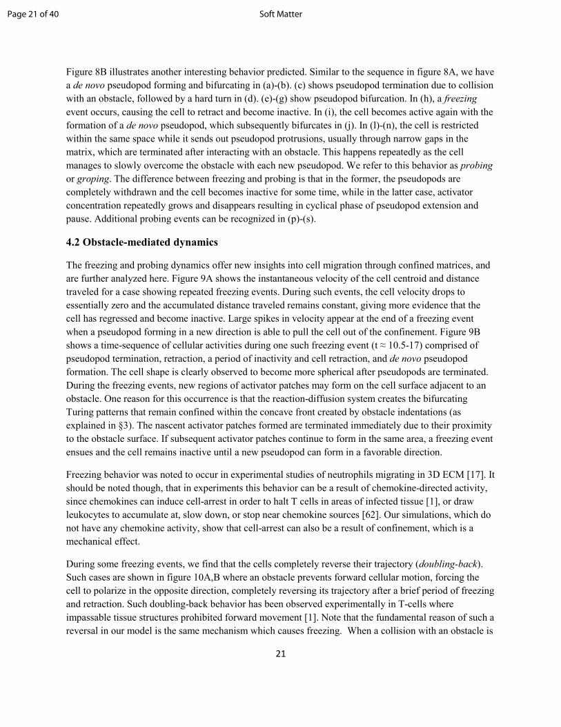
The freezing and probing dynamics offer new insights into cell migration through confined matrices, and

are further analyzed here. Figure 9A shows the instantaneous velocity of the cell centroid and distance

traveled for a case showing repeated freezing events. During such events, the cell velocity drops to

essentially zero and the accumulated distance traveled remains constant, giving more evidence that the

cell has regressed and become inactive. Large spikes in velocity appear at the end of a freezing event

when a pseudopod forming in a new direction is able to pull the cell out of the confinement. Figure 9B

shows a time-sequence of cellular activities during one such freezing event (t ≈ 10.5-17) comprised of

pseudopod termination, retraction, a period of inactivity and cell retraction, and de novo pseudopod

formation. The cell shape is clearly observed to become more spherical after pseudopods are terminated.

During the freezing events, new regions of activator patches may form on the cell surface adjacent to an

obstacle. One reason for this occurrence is that the reaction-diffusion system creates the bifurcating

Turing patterns that remain confined within the concave front created by obstacle indentations (as

explained in §3). The nascent activator patches formed are terminated immediately due to their proximity

to the obstacle surface. If subsequent activator patches continue to form in the same area, a freezing event

ensues and the cell remains inactive until a new pseudopod can form in a favorable direction.

Freezing behavior was noted to occur in experimental studies of neutrophils migrating in 3D ECM [17]. It

should be noted though, that in experiments this behavior can be a result of chemokine-directed activity,

since chemokines can induce cell-arrest in order to halt T cells in areas of infected tissue [1], or draw

leukocytes to accumulate at, slow down, or stop near chemokine sources [62]. Our simulations, which do

not have any chemokine activity, show that cell-arrest can also be a result of confinement, which is a

mechanical effect.

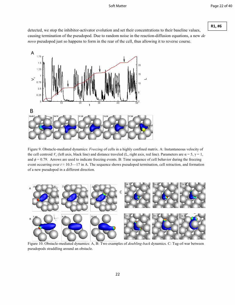
During some freezing events, we find that the cells completely reverse their trajectory (doubling-back).

Such cases are shown in figure 10A,B where an obstacle prevents forward cellular motion, forcing the

cell to polarize in the opposite direction, completely reversing its trajectory after a brief period of freezing

and retraction. Such doubling-back behavior has been observed experimentally in T-cells where

impassable tissue structures prohibited forward movement [1]. Note that the fundamental reason of such a

reversal in our model is the same mechanism which causes freezing. When a collision with an obstacle is


22

detected, we stop the inhibitor-activator evolution and set their concentrations to their baseline values,

causing termination of the pseudopod. Due to random noise in the reaction-diffusion equations, a new de

novo pseudopod just so happens to form in the rear of the cell, thus allowing it to reverse course.

Figure 9. Obstacle-mediated dynamics: Freezing of cells in a highly confined matrix. A: Instantaneous velocity of

the cell centroid Vc (left axis, black line) and distance traveled (L, right axis, red line). Parameters are α = 5, γ = 1,

and ϕ = 0.79. Arrows are used to indicate freezing events. B: Time sequence of cell behavior during the freezing

event occurring over t ≈ 10.5—17 in A. The sequence shows pseudopod termination, cell retraction, and formation

of a new pseudopod in a different direction.

Figure 10. Obstacle-mediated dynamics: A, B: Two examples of doubling-back dynamics. C: Tug-of-war between

pseudopods straddling around an obstacle.

R1, #6


23

Another interesting behavior observed in our simulations occurs when a cell adjacent to an obstacle

generates a pseudopod which bifurcates and forks around both sides of the obstacle. The two pseudopods

then compete, and a resulting tug-of-war ensues until one pseudopod wins and carries the cell forward

(figure 10C). The cell is seen to wrap around the obstacle before one pseudopod retracts. Experiments

involving neutrophils in vitro have observed this behavior, noting there was no significant bias in the

direction cells chose [63].

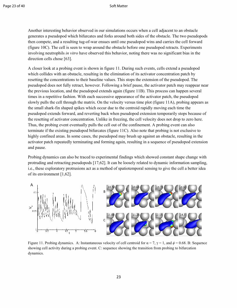
A closer look at a probing event is shown in figure 11. During such events, cells extend a pseudopod

which collides with an obstacle, resulting in the elimination of its activator concentration patch by

resetting the concentrations to their baseline values. This stops the extension of the pseudopod. The

pseudopod does not fully retract, however. Following a brief pause, the activator patch may reappear near

the previous location, and the pseudopod extends again (figure 11B). This process can happen several

times in a repetitive fashion. With each successive appearance of the activator patch, the pseudopod

slowly pulls the cell through the matrix. On the velocity versus time plot (figure 11A), probing appears as

the small shark-fin shaped spikes which occur due to the centroid rapidly moving each time the

pseudopod extends forward, and reverting back when pseudopod extension temporarily stops because of

the resetting of activator concentration. Unlike in freezing, the cell velocity does not drop to zero here.

Thus, the probing event eventually pulls the cell out of the confinement. A probing event can also

terminate if the existing pseudopod bifurcates (figure 11C). Also note that probing is not exclusive to

highly confined areas. In some cases, the pseudopod may brush up against an obstacle, resulting in the

activator patch repeatedly terminating and forming again, resulting in a sequence of pseudopod extension

and pause.

Probing dynamics can also be traced to experimental findings which showed constant shape change with

protruding and retracting pseudopods [17,62]. It can be loosely related to dynamic information sampling,

i.e., these exploratory protrusions act as a method of spatiotemporal sensing to give the cell a better idea

of its environment [1,62].

Figure 11. Probing dynamics. A: Instantaneous velocity of cell centroid for α = 7, γ = 1, and ϕ = 0.68. B: Sequence

showing cell activity during a probing event. C: sequence showing the transition from probing to bifurcation

dynamics.


24

4.3 Limits on motility

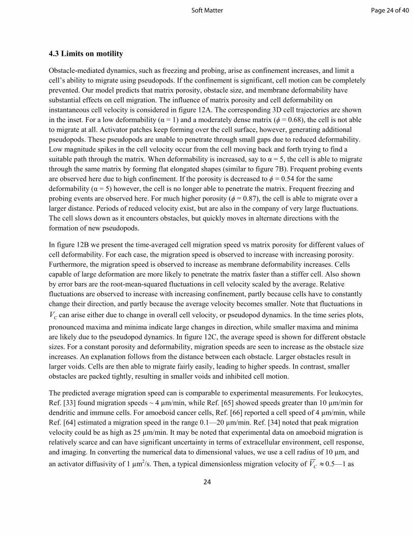
Obstacle-mediated dynamics, such as freezing and probing, arise as confinement increases, and limit a

cell’s ability to migrate using pseudopods. If the confinement is significant, cell motion can be completely

prevented. Our model predicts that matrix porosity, obstacle size, and membrane deformability have

substantial effects on cell migration. The influence of matrix porosity and cell deformability on

instantaneous cell velocity is considered in figure 12A. The corresponding 3D cell trajectories are shown

in the inset. For a low deformability (α = 1) and a moderately dense matrix (ϕ = 0.68), the cell is not able

to migrate at all. Activator patches keep forming over the cell surface, however, generating additional

pseudopods. These pseudopods are unable to penetrate through small gaps due to reduced deformability.

Low magnitude spikes in the cell velocity occur from the cell moving back and forth trying to find a

suitable path through the matrix. When deformability is increased, say to α = 5, the cell is able to migrate

through the same matrix by forming flat elongated shapes (similar to figure 7B). Frequent probing events

are observed here due to high confinement. If the porosity is decreased to ϕ = 0.54 for the same

deformability (α = 5) however, the cell is no longer able to penetrate the matrix. Frequent freezing and

probing events are observed here. For much higher porosity (ϕ = 0.87), the cell is able to migrate over a

larger distance. Periods of reduced velocity exist, but are also in the company of very large fluctuations.

The cell slows down as it encounters obstacles, but quickly moves in alternate directions with the

formation of new pseudopods.

In figure 12B we present the time-averaged cell migration speed vs matrix porosity for different values of

cell deformability. For each case, the migration speed is observed to increase with increasing porosity.

Furthermore, the migration speed is observed to increase as membrane deformability increases. Cells

capable of large deformation are more likely to penetrate the matrix faster than a stiffer cell. Also shown

by error bars are the root-mean-squared fluctuations in cell velocity scaled by the average. Relative

fluctuations are observed to increase with increasing confinement, partly because cells have to constantly

change their direction, and partly because the average velocity becomes smaller. Note that fluctuations in

CV can arise either due to change in overall cell velocity, or pseudopod dynamics. In the time series plots,

pronounced maxima and minima indicate large changes in direction, while smaller maxima and minima

are likely due to the pseudopod dynamics. In figure 12C, the average speed is shown for different obstacle

sizes. For a constant porosity and deformability, migration speeds are seen to increase as the obstacle size

increases. An explanation follows from the distance between each obstacle. Larger obstacles result in

larger voids. Cells are then able to migrate fairly easily, leading to higher speeds. In contrast, smaller

obstacles are packed tightly, resulting in smaller voids and inhibited cell motion.

The predicted average migration speed can is comparable to experimental measurements. For leukocytes,

Ref. [33] found migration speeds ~ 4 µm/min, while Ref. [65] showed speeds greater than 10 µm/min for

dendritic and immune cells. For amoeboid cancer cells, Ref. [66] reported a cell speed of 4 µm/min, while

Ref. [64] estimated a migration speed in the range 0.1—20 µm/min. Ref. [34] noted that peak migration

velocity could be as high as 25 µm/min. It may be noted that experimental data on amoeboid migration is

relatively scarce and can have significant uncertainty in terms of extracellular environment, cell response,

and imaging. In converting the numerical data to dimensional values, we use a cell radius of 10 µm, and

an activator diffusivity of 1 µm2/s. Then, a typical dimensionless migration velocity of ≈CV 0.5—1 as


25

obtained from figure 12B for moderate values of matrix porosity, obstacle size and cell deformability

yields a dimensional speed of 3—6 µm/min. This is in agreement with the range of experimentally

measured speeds.

Figure 12. A: Influence of matrix porosity and cell deformability on instantaneous cell velocity and cell trajectory

(inset). B: Time averaged migration speed as a function of matrix porosity for different cell deformabilities. C: Time

averaged migration speed as a function of matrix porosity for different obstacle size. The error bars represent rms

velocity fluctuation.


26

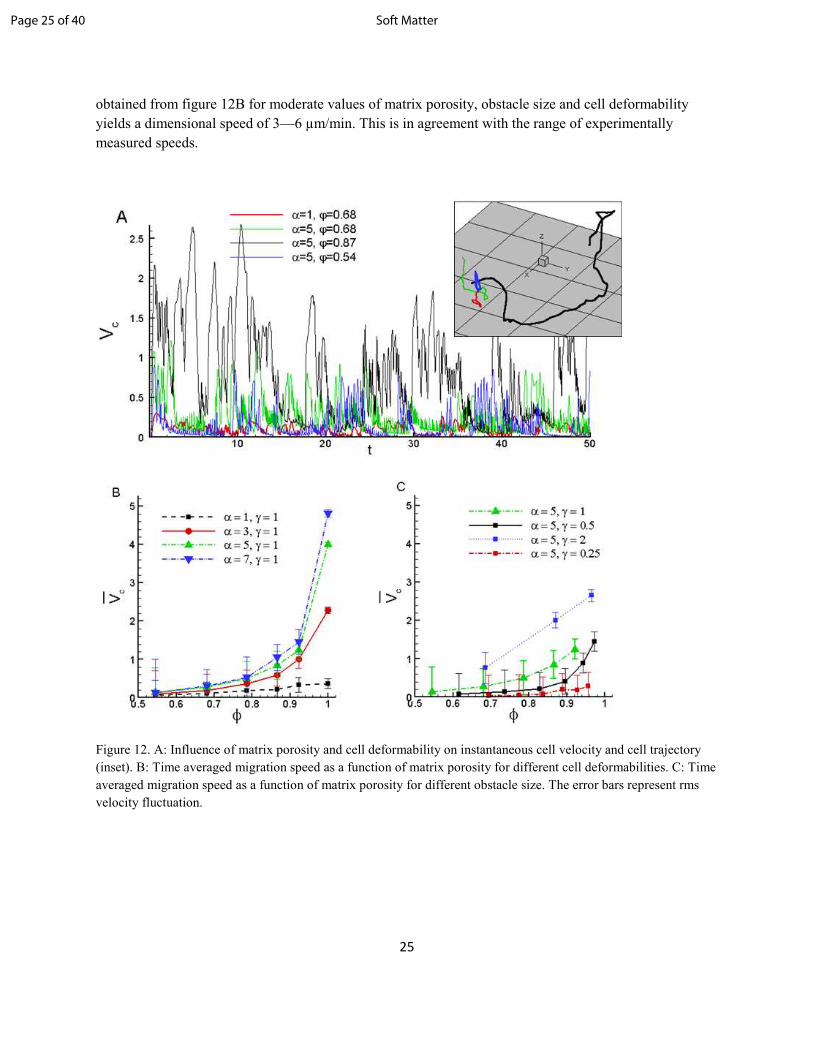
As figure 12 shows, cell migration becomes increasingly hindered with decreasing porosity, cell

deformability, and obstacle size. Below certain values of these parameters, cell penetration through the

matrix will not be possible. Such “motility limits” for the current matrix are shown in figure 13. It shows

that for a given porosity and obstacle size, migration is possible only if the cells are deformable enough.

Similarly, for a given deformability, migration can occur only if the matrix porosity is sufficient. It further

shows that obstacles of smaller size can also result in cell arrest. These results are qualitatively similar to

experimental observations. Neutrophils, for instance, are capable of squeezing through very tight spaces

due to their soft membranes, while the stiffer fibroblasts cannot [2], and must use other means to move

through the body such as matrix remodeling [64].

Figure 13. Motility limits as obtained from the current simulations. Phase diagrams are shown in terms for

confinement (1― ϕ) and cell deformability for three different obstacle sizes. Open squares represent cases for which

cells are able to migrate through the matrix, and filled circles represent cases when cell movement is prevented.

4.4 Pseudopod dynamics

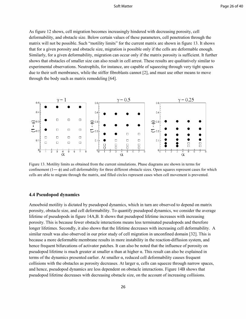
Amoeboid motility is dictated by pseudopod dynamics, which in turn are observed to depend on matrix

porosity, obstacle size, and cell deformability. To quantify pseudopod dynamics, we consider the average

lifetime of pseudopods in figure 14A,B. It shows that pseudopod lifetime increases with increasing

porosity. This is because fewer obstacle interactions means less terminated pseudopods and therefore

longer lifetimes. Secondly, it also shows that the lifetime decreases with increasing cell deformability. A

similar result was also observed in our prior study of cell migration in unconfined domain [32]. This is

because a more deformable membrane results in more instability in the reaction-diffusion system, and

hence frequent bifurcations of activator patches. It can also be noted that the influence of porosity on

pseudopod lifetime is much greater at smaller α than at higher α. This result can also be explained in

terms of the dynamics presented earlier. At smaller α, reduced cell deformability causes frequent

collisions with the obstacles as porosity decreases. At larger α, cells can squeeze through narrow spaces,

and hence, pseudopod dynamics are less dependent on obstacle interactions. Figure 14B shows that

pseudopod lifetime decreases with decreasing obstacle size, on the account of increasing collisions.


27

Another important pseudopod characteristic is the number of de novo pseudopods produced. As noted

before, a pseudopod can generate either from a freshly formed activator patch that has not bifurcated

previously, or from bifurcation of an existing pseudopod. The de novo pseudopods are defined as those

generated by the first mechanism. Figure 14C,D shows the percentage of the de novo pseudopods of the

total formed by both mechanisms. It can be observed that the fraction of de novo pseudopods increases

with decreasing porosity. Cells encountering a greater number of obstacles in a low porosity environment

have more pseudopods terminated (due to frequent resetting of activator and inhibitor concentrations to

their baseline values). New pseudopods are then generated more frequently in order for the cell to

migrate. Also, for a given porosity, the fraction of de novo pseudopods increases with increasing cell

deformability. A decreasing obstacle size also results in more de novo pseudopods. The explanation for

these results directly follow from the one given above for the pseudopod lifetime.

Figure 14. Pseudopod lifetime τP (scaled by R2/D1) as a function of α for different values of matrix porosity (A),

and as a function of obstacle size (B). Fraction of de novo pseudopods to total pseudopods as a function of α for

different values of matrix porosity (C), and as a function of obstacle size (D).


28

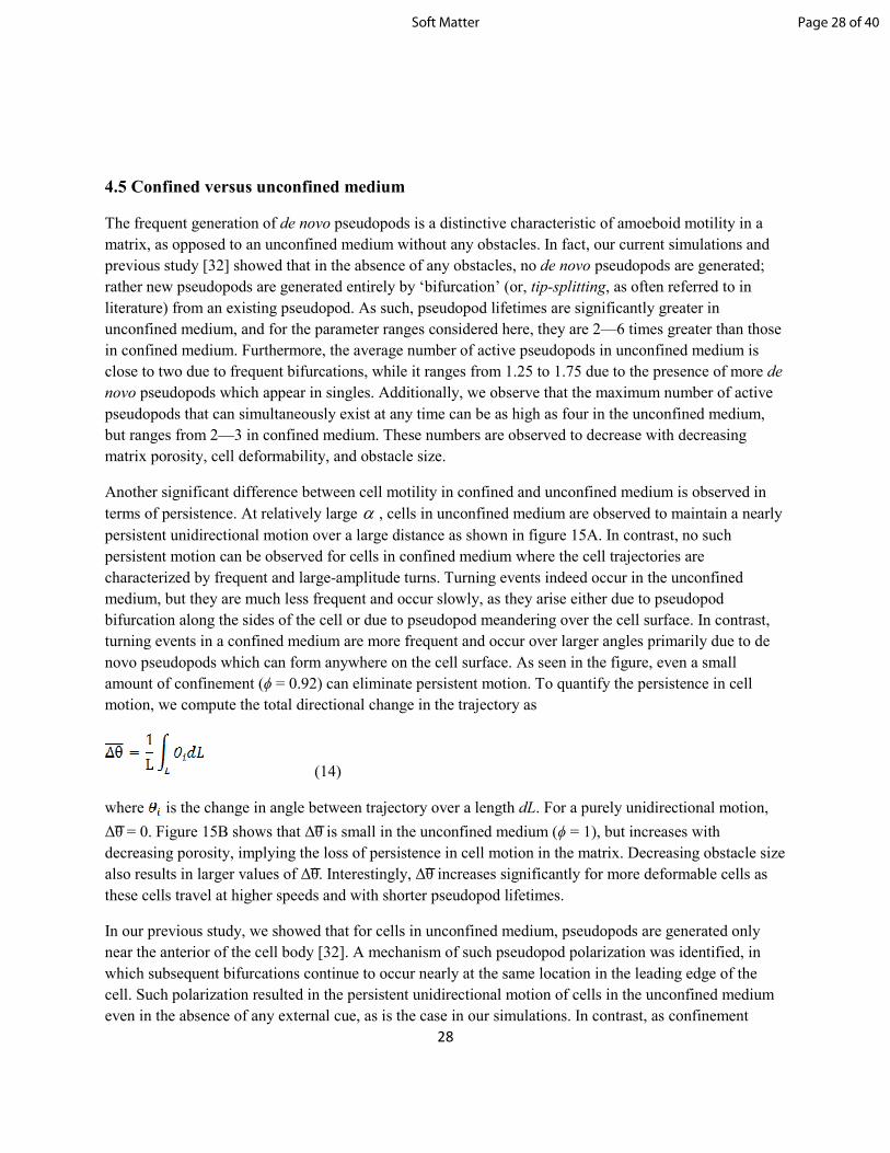
4.5 Confined versus unconfined medium

The frequent generation of de novo pseudopods is a distinctive characteristic of amoeboid motility in a

matrix, as opposed to an unconfined medium without any obstacles. In fact, our current simulations and

previous study [32] showed that in the absence of any obstacles, no de novo pseudopods are generated;

rather new pseudopods are generated entirely by ‘bifurcation’ (or, tip-splitting, as often referred to in

literature) from an existing pseudopod. As such, pseudopod lifetimes are significantly greater in

unconfined medium, and for the parameter ranges considered here, they are 2—6 times greater than those

in confined medium. Furthermore, the average number of active pseudopods in unconfined medium is

close to two due to frequent bifurcations, while it ranges from 1.25 to 1.75 due to the presence of more de

novo pseudopods which appear in singles. Additionally, we observe that the maximum number of active

pseudopods that can simultaneously exist at any time can be as high as four in the unconfined medium,

but ranges from 2—3 in confined medium. These numbers are observed to decrease with decreasing

matrix porosity, cell deformability, and obstacle size.

Another significant difference between cell motility in confined and unconfined medium is observed in

terms of persistence. At relatively large α , cells in unconfined medium are observed to maintain a nearly

persistent unidirectional motion over a large distance as shown in figure 15A. In contrast, no such

persistent motion can be observed for cells in confined medium where the cell trajectories are

characterized by frequent and large-amplitude turns. Turning events indeed occur in the unconfined

medium, but they are much less frequent and occur slowly, as they arise either due to pseudopod

bifurcation along the sides of the cell or due to pseudopod meandering over the cell surface. In contrast,

turning events in a confined medium are more frequent and occur over larger angles primarily due to de

novo pseudopods which can form anywhere on the cell surface. As seen in the figure, even a small

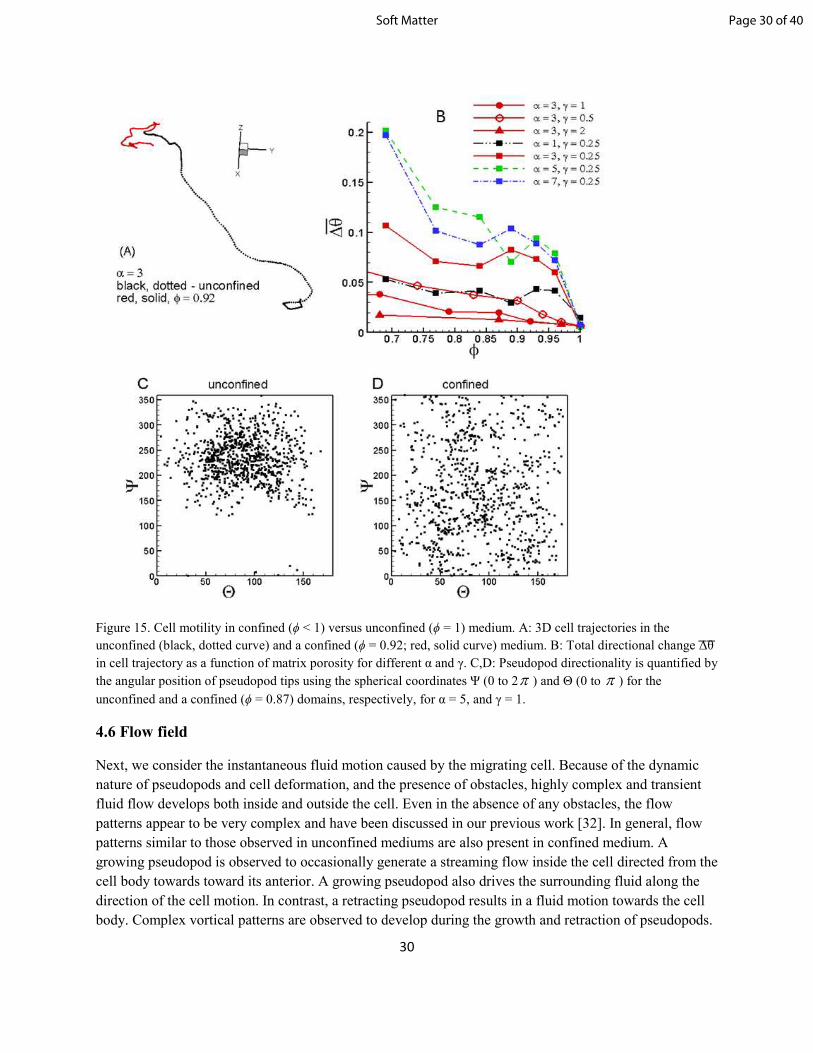
amount of confinement (ϕ = 0.92) can eliminate persistent motion. To quantify the persistence in cell

motion, we compute the total directional change in the trajectory as

(14)

where is the change in angle between trajectory over a length dL. For a purely unidirectional motion,

∆͞θ = 0. Figure 15B shows that ∆͞θ is small in the unconfined medium (ϕ = 1), but increases with

decreasing porosity, implying the loss of persistence in cell motion in the matrix. Decreasing obstacle size

also results in larger values of ∆͞θ. Interestingly, ∆͞θ increases significantly for more deformable cells as

these cells travel at higher speeds and with shorter pseudopod lifetimes.

In our previous study, we showed that for cells in unconfined medium, pseudopods are generated only

near the anterior of the cell body [32]. A mechanism of such pseudopod polarization was identified, in

which subsequent bifurcations continue to occur nearly at the same location in the leading edge of the

cell. Such polarization resulted in the persistent unidirectional motion of cells in the unconfined medium

even in the absence of any external cue, as is the case in our simulations. In contrast, as confinement


29

increases, the number of de novo pseudopods increases. Such de novo pseudopods appear all over the cell

surface without any directional preference due to the random noise in the reaction-diffusion system. To

quantify pseudopod polarization, we compute the angular position of pseudopod tips using the spherical

angles Ψ and Θ as shown in figure 15C, D. Ψ and Θ are spherical coordinates measuring the outward

normal vector of active pseudopods. They are absolute coordinates using the Eulerian Cartesian system as

a frame of reference. Ψ is the angle of the pseudopod normal projected onto the xy plane, relative to the

x-axis, while Θ is the angle off the z-axis. Each data point represents the direction of an active pseudopod

at a specific time step. Because pseudopods are force generators, cells tend to move in the direction the

pseudopod points. Therefore, the orientation of the pseudopods determines the track the cell will take. For

the cell in unconfined medium (figure 15C), a tight grouping of data points in a small range of Ψ is

observed, which indicates that pseudopods are focused and generated in nearly the same direction. The

reason for the tight grouping for the unconfined case was studied in details in our previous work [32]. A

brief explanation is as follows: in an unconfined space, the same bifurcating pattern continues as there is

no need for resetting the activator /inhibitor concentrations. Because of its own instability (§3.1), an

activator patch located near the front of the cell bifurcates before it can travel significantly over the cell

surface. As such, the activator patches remain within the front part f the cell, thereby creating a focused

distribution of the activator patches. The resulting pseudopods, therefore, remain focused as well,

generating the angular bias for the unconfined case. In contrast, for the cell in confined medium (figure

15D), a uniformly scattered distribution is noted, which indicates that pseudopods are generated around

the entire cell surface in all directions. Again, this is because the RD process is terminated every time a

cell gets stuck around an obstacle. As evident in the figure, even a small amount of confinement (ϕ =

0.87) is sufficient to break the polarity of the pseudopods. This loss of polarization is due to the frequent

collision of the pseudopods with the obstacles, and results in the loss of persistence in cell motion in the

matrix.

R1, #7


30

Figure 15. Cell motility in confined (ϕ < 1) versus unconfined (ϕ = 1) medium. A: 3D cell trajectories in the

unconfined (black, dotted curve) and a confined (ϕ = 0.92; red, solid curve) medium. B: Total directional change ͞∆͞θ

in cell trajectory as a function of matrix porosity for different α and γ. C,D: Pseudopod directionality is quantified by

the angular position of pseudopod tips using the spherical coordinates Ψ (0 to 2π ) and Θ (0 to π ) for the

unconfined and a confined (ϕ = 0.87) domains, respectively, for α = 5, and γ = 1.

4.6 Flow field

Next, we consider the instantaneous fluid motion caused by the migrating cell. Because of the dynamic

nature of pseudopods and cell deformation, and the presence of obstacles, highly complex and transient

fluid flow develops both inside and outside the cell. Even in the absence of any obstacles, the flow

patterns appear to be very complex and have been discussed in our previous work [32]. In general, flow

patterns similar to those observed in unconfined mediums are also present in confined medium. A

growing pseudopod is observed to occasionally generate a streaming flow inside the cell directed from the

cell body towards toward its anterior. A growing pseudopod also drives the surrounding fluid along the

direction of the cell motion. In contrast, a retracting pseudopod results in a fluid motion towards the cell

body. Complex vortical patterns are observed to develop during the growth and retraction of pseudopods.


31

Microswimmers of well-defined shapes under harmonic motion are often classified as pushers and pullers

depending on their swimming patterns. Pushers repel fluid along the direction of swimming, but attract it

along the sides, while pullers draw fluid towards the swimming direction but repel fluid outwards along

the sides. In our simulations, pusher motion is rarely seen, and only during the initial transience. Puller

motion, on the other hand, is seen more often in our simulations. In general however, the cell behavior

cannot be uniquely classified as pusher or puller because of the highly deformed cell shape and the

dynamic nature of the pseudopods.

Additionally, some unique features are also observed in the flow patterns in confined medium that are not

present in unconfined medium. Specifically, vortices rotating in alternating directions are observed to

form during pseudopod growth and retraction in confined medium. A sequence of such events is shown in

figure 16(A--F) for a matrix of ϕ = 0.54. Here in (A), two clockwise vortices (shown by locations A and

B) form during pseudopod growth and bifurcation. These pseudopods are terminated in (B) as they

encounter obstacles, and their retraction generates two counter-clockwise vortices. Two clockwise

vortices are generated again in (E-F) as new pseudopods are formed. Such alternating sequence of

vortices is a result of repeated formation of de novo pseudopods and their termination due to the presence

of the obstacles. As such, these patterns are absent in an unconfined medium, and occur more frequently

with increasing confinement. Another example is shown in sequence (G—J) that corresponds to a probing

event. Here, counter-rotating vortices are observed on both sides of a growing pseudopod. As the

pseudopod repeatedly extends and retracts, vortices generated during the extension phase reverse

direction during the retraction phase.


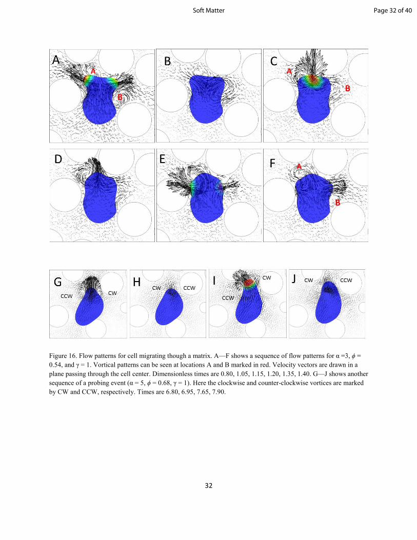
32

Figure 16. Flow patterns for cell migrating though a matrix. A—F shows a sequence of flow patterns for α =3, ϕ =

0.54, and γ = 1. Vortical patterns can be seen at locations A and B marked in red. Velocity vectors are drawn in a

plane passing through the cell center. Dimensionless times are 0.80, 1.05, 1.15, 1.20, 1.35, 1.40. G—J shows another

sequence of a probing event (α = 5, ϕ = 0.68, γ = 1). Here the clockwise and counter-clockwise vortices are marked

by CW and CCW, respectively. Times are 6.80, 6.95, 7.65, 7.90.


33

5. ADDITIONAL CONSIDERATIONS

5.1 Viscoelastic membrane

In our previous work [29], we have developed a highly-accurate model for viscoelastic

membrane. The viscoelastic behavior is resolved using the Kelvin-Voigt model in which the total

membrane stress is expressed as the sum of the elastic and viscous stresses as

where the elastic stress is given by Eq. 2, and the viscous stress is expressed as

where µm is membrane shear viscosity (~10

‒7―10

‒6 N.s/m, [29]), D is the strain rate tension, and

Is is the surface projection tensor. For numerical implementation, the stress is computed in terms

of the strain history using a time-convolution integral. Simulations of cell motility are performed

by considering three different values of dimensionless membrane viscosity as µm/µ0 R = 0, 1, and

10, with zero being the elastic membrane. These results are given in the Supplementary Materials

(figure S2). The dimensionless average cell speed shows a small increase with increasing

membrane viscosity (from ~ 0.4 to 0.6), and the RMS velocity fluctuation shows a small

decrease. The persistence was also similar, with the total directional change ͞∆θ being 0.026,

0.021, and 0.020, respectively. The general motility behavior remains similar. The obstacle-

mediated dynamics, namely, the freezing and probing was also observed. Viscosity stiffens the

membrane, and causes ruffles that are footprints of dead pseudopods (see Supplementary

Materials, figure S3). These ruffles are high curvature regions, and hence, they cause more

frequent bifurcation of activator patches as noted in §3.2. As a result, the number of pseudopods

slightly increases resulting in higher speed. Note that the time scale for membrane deformation R

µ0 / GS ~ µm/GS ~ 10‒3

―10‒2

s, while the time scale for activator/inhibitor diffusion R2/D3 or

R2/D1 ~ 1s. So, the membrane quickly responds to the evolving Turing patterns, even when the

viscosity is relatively large, and the cell behavior is essentially dictated by the activator/inhibitor

dynamics.

5.2 Variation of bending rigidity

The nonlinear constitutive law (Eq. 1) used to model membrane deformation is known to create

membrane buckling [29]. Also, the protrusive force can cause sharp kinks. To avoid these,

membrane bending is needed. The bending stiffness EB typically is in the range 1―9 X 10‒19

J

[36,57]. The corresponding dimensionless parameter is EB* = EB/R

2 GS . Simulations were

performed by varying EB* as 0.003 to 0.02, and the average cell speed is given in the

Supplementary materials (figure S4). Cell velocities had no significant deviations, nor did the

persistence as defined by Eq. 14. Cell dynamics were also similar with comparable trajectories.

In addition, obstacle-mediated dynamics, such as probing and freezing, were also observed.

R1, #2

R1, #4


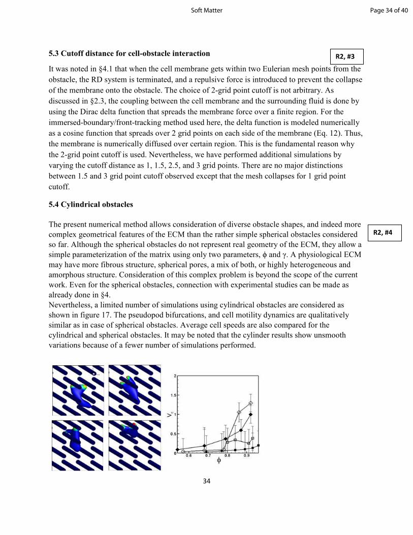
34

5.3 Cutoff distance for cell-obstacle interaction

It was noted in §4.1 that when the cell membrane gets within two Eulerian mesh points from the

obstacle, the RD system is terminated, and a repulsive force is introduced to prevent the collapse

of the membrane onto the obstacle. The choice of 2-grid point cutoff is not arbitrary. As

discussed in §2.3, the coupling between the cell membrane and the surrounding fluid is done by

using the Dirac delta function that spreads the membrane force over a finite region. For the

immersed-boundary/front-tracking method used here, the delta function is modeled numerically

as a cosine function that spreads over 2 grid points on each side of the membrane (Eq. 12). Thus,

the membrane is numerically diffused over certain region. This is the fundamental reason why

the 2-grid point cutoff is used. Nevertheless, we have performed additional simulations by

varying the cutoff distance as 1, 1.5, 2.5, and 3 grid points. There are no major distinctions

between 1.5 and 3 grid point cutoff observed except that the mesh collapses for 1 grid point

cutoff.

5.4 Cylindrical obstacles

The present numerical method allows consideration of diverse obstacle shapes, and indeed more

complex geometrical features of the ECM than the rather simple spherical obstacles considered

so far. Although the spherical obstacles do not represent real geometry of the ECM, they allow a

simple parameterization of the matrix using only two parameters, ϕ and γ. A physiological ECM

may have more fibrous structure, spherical pores, a mix of both, or highly heterogeneous and

amorphous structure. Consideration of this complex problem is beyond the scope of the current

work. Even for the spherical obstacles, connection with experimental studies can be made as

already done in §4.

Nevertheless, a limited number of simulations using cylindrical obstacles are considered as

shown in figure 17. The pseudopod bifurcations, and cell motility dynamics are qualitatively

similar as in case of spherical obstacles. Average cell speeds are also compared for the

cylindrical and spherical obstacles. It may be noted that the cylinder results show unsmooth

variations because of a fewer number of simulations performed.

R2, #3

R2, #4


35

Figure 17. Influence of cylindrical obstacles. Snapshots show a sequence of motility. The

average cell speed is compared for cylinders (open symbols) and spheres (filled symbols) for γ =

1 (diamonds), and 0.25 (squares).

6. CONCLUSIONS

We presented a 3D multiscale and multiphysics computational model coupling fluid mechanics, solid

mechanics, and dynamic pattern formation to simulate locomotion of amoeboid cells through a porous

extra-cellular space. The extracellular space is made of a viscous fluid and an array of finite-size, rigid,

non-moving spherical obstacles. Amoeboid cells migrate by extending pseudopods, and undergoing

extreme deformation. We use an immersed-boundary method (IBM), which is efficient in resolving

extreme deformation, and allows a seamless integration of diverse types of interfaces, both deformable

and rigid. The model combines reaction/diffusion of activator/inhibitors, extreme deformation of the cell,

pseudopod dynamics, cytoplasmic and extracellular fluid motion, and a fully resolved extracellular

environment. Cell deformation is numerically computed using a surface finite element method, and the

fluid motion is solved using a combined finite-volume and spectral method. An evolving surface finite-

element method is also used to solve the non-linear reaction-diffusion equations for the activator-inhibitor

dynamics. The dynamic nature of the Turing instability in the activator-inhibitor model allows us to

evolve protein concentration on the cell membrane, which is then correlated to the protrusive force. A

continuous forcing IBM is used to couple cell deformation with the fluid, while a direct forcing IBM is

used for obstacle—fluid coupling. In the model, the receptor-ligand bond formation between the cell and

an obstacle is not considered. Furthermore, no external cue such as a chemical gradient is applied.

The model is able to recreate pseudopod-driven motility of a cell through the matrix. The predicted cell

shapes are similar to those observed in experiments. The dynamics of pseudopods, namely their

generation, bifurcation, meandering, and retraction are accurately predicted by the model. Extreme

deformation of the cells is reliably predicted as they squeeze and weave through the narrow spaces

between obstacles over long simulation times suggesting robustness of the methodology. Additionally,

the predicted migration velocity is in agreement with the range reported in experimental studies.

We presented a detailed mechanistic view of how amoeboid cells negotiate around obstacles. Toward that

end, we studied the influence of matrix porosity, obstacle size, and cell deformability on the cell motility

behavior. All of these parameters are shown to strongly affect cell migration. We show that below certain

values of these parameters, cell motion can be completely prevented. Cells must be sufficiently

deformable to squeeze through narrow spaces between obstacles. Based on our simulations, we present

phase diagrams of motility limits for the cell—matrix combination considered here. Existence of such

motility limits can be inferred from experimental studies. For example, softer immune cells are known to

easily migrate through tissue, while stiffer fibroblasts move with an order of magnitude slower speed.

Furthermore, our model predicts interesting motility behaviors that are caused by the obstacles, namely

freezing, probing, doubling-back, and tug-of-war. The freezing event is characterized by a temporary

pause in cell motion, while in probing the cell repeatedly extends and retracts its pseudopod as if to

sample its surroundings. The doubling-back and tug-of-war dynamics allow the cell to get out of a

R1, #8


36

confined region and continue its migration. These dynamics are absent in unconfined medium, and they

appear more frequently with decreasing matrix porosity. Only a few experimental studies have suggested

the presence of such dynamics, but attributed them to signaling proteins. In contrast, our model shows

that such dynamics could be of mechanistic origins.

The model predicts that in the unconfined medium, cells exhibit persistent unidirectional motion over

long times. Such persistent unidirectional motion of amoeboid cells in the absence of any external

chemoattractant gradient was reported in experimental studies [9,44]. Here, and in our previous study

[32], we showed that such persistent motion is due to the polarization of pseudopods near the anterior of

the cell. This persistent motion, however, is shown to be lost in the presence of obstacles as the cells

migrate with a zig-zag pattern. We show that the loss of persistence is due to a major alteration in the

pseudopod dynamics. In the unconfined medium, new pseudopods are generated only by bifurcation of an

existing pseudopod. In contrast, in a confined medium, an existing pseudopod is often terminated as it

collides with an obstacle. As such, the cells in a confined medium migrate primarily by forming de novo

pseudopods. A de novo pseudopod is generated from a new activator patch which can form anywhere on

the cell surface due to the random noise in the reaction-diffusion system. Our simulations predict that the

fraction of such de novo pseudopods increases with increasing confinement. Increasing confinement also

results in a decreasing lifetime of the pseudopods. The increase in randomly generated de novo

pseudopods and their shorter lifetimes result in frequent direction changes and hard turns in the cell

trajectory in a confined medium. While this mechanism causes the loss of persistence in the motion, it

also allows the cell to find a new direction, without which it would be unable to migrate through the

matrix. Additionally, we find that the average and maximum number of pseudopods are reduced in

presence of confinement, as well as with decreasing matrix porosity.

Inclusion of fluid interaction enables us to extract instantaneous 3D velocity fields both inside and outside

the migrating cells. In general, highly complex and dynamic flow patterns are observed, even in the

absence of any obstacles. Some unique features are also observed in the flow patterns in confined medium

that are not present in the unconfined medium. Specifically, vortices rotating in alternating directions are

observed to form during pseudopod growth and retraction. Such flow patterns generated by the motion of

the cell itself can alter the distribution of the extracellular molecules and chemoattractants.

In conclusion, the current study presents a fully 3D, robust numerical model for pseudopod-driven

motility of highly deformable amoeboid cells through an extracellular medium. The results and analysis

presented here provide new insights on cell motility in confined medium. They show a strong coupling

between cell deformability and ECM properties in dictating motility behavior. These results could also be

useful in designing artificial tissue scaffolds where controlled cell migration may be desired. While in this

work we considered a rather simple extracellular scaffold, the numerical method is not limited to such

specific geometry. Highly complex and physiologically realistic scaffolds can be considered, and will be

addressed in our future studies.

Supplemental Materials: Additional results and an animation from one simulation is provided.


37

Acknowledgement: The work is supported by grant CBET 1438255 from the National Science

Foundation, and Peter B. Cherasia fund from Rutgers. Computational resources from NSF’s XSEDE

resources at TACC are acknowledged.

References

1. A. Gaylo, D. C. Schrock, N. R. J. Fernandes, and D. J. Fowell, T Cell Interstitial Migration:

Motility Cues from the Inflamed Tissue for Micro- and Macro-Positioning, Frontiers in

Immunology 7, (2016).

2. R. J. Petrie and K. M. Yamada, Fibroblasts Lead the Way: A Unified View of 3D Cell Motility,

Trends in Cell Biol. 25, 666 (2015).

3. M. Scianna, An extended Cellular Potts Model analyzing a wound healing assay, Comput. in

Biol. and Medicine 62, 33 (2015).

4. E. Raz and H. Mahabaleshwar, Chemokine signaling in embryonic cell migration: a fisheye view,

Development 136, 1223 (2009).

5. A. Wells, J. Grahovac, S. Wheeler, B. Ma, and D. Lauffenburger, Targeting tumor cell motility as

a strategy against invasion and metastasis, Trends in Pharmacological Sci. 34, 283 (2013).

6. D. Bray, Cell movements: From molecules to motility (New York, 2000).

7. N. P. Barry and M. S. Bretscher, Dictyostelium amoeba and neutrophils can swim, Proc. Natl.

Acad. Sci. USA 107, 11376 (2010).

8. A. J. Bae and E. Bodenschatz, On the swimming of Dictyostelium amoebae, Proc. Natl. Acad.

Sci. USA 107, E165 (2010).

9. P. J. M. Van Haastert, Amoeboid cells use protrusions for walking, gliding and swimming, PLoS

ONE, 6, e27532 (2011).

10. M. M. Stevens and J. H. George, Exploring and Engineering the Cell Surface Interface, Science

310, 1135 (2005).

11. C. D. Paul, P. Mistriotis, and K. Konstantopoulos, Cancer cell motility: lessons from migration in

confined spaces, Nature Rev. Cancer 17, 131 (2017).

12. M. Sixt and T. Lämmermann, In Vitro Analysis of Chemotactic Leukocyte Migration in 3D

Environments, Methods in Molecular Biol. 769, 149 (2011).

13. H. Yamaguchi, J. Wyckoff, and J. Condeelis, Cell migration in tumors, Curr. Opin. Cell Biol. 17,

559 (2005).

14. K. Wolf, S. Alexander, V. Schacht, L. M. Coussens, U. H. von Andrian, J. van Rheenen, E.

Deryugina, and P. Friedl, Collagen-based cell migration models in vitro and in vivo, Seminars in

Cell and Developmental Biol. 20, 931 (2009).

15. R. J. Huber and D. H. O’Day, Extracellular matrix dynamics and functions in the social amoeba

Dictyostelium: A critical review, Biochimica et Biophysica Acta 1861, 2971 (2017).

16. Y. J. Liu, M. Le Berre, R. Voituriez, and M. Piel, Confinement and Low Adhesion Induce Fast

Amoeboid Migration of Slow Mesenchymal Cells, Cell 160, 659 (2015).

17. J. T. H. Mandeville, M. A. Lawson, and F. R. Maxfield, Dynamic imaging of neutrophil

migration in three dimensions: mechanical interactions between cells and matrix, J. Leukocyte

Biol. 61, 188 (1997).


38

18. K. Wolf, I. Mazo, H. Leung, K. Engelke, U. H. von Andrian, E. I. Deryugina, A. Y. Strongin, E.

B. Bröcker, and P. Friedl, Compensation mechanism in tumor cell migration: mesenchymal-

amoeboid transition after blocking of pericellular proteolysis, J. Cell Biol. 160, 267 (2003).

19. H. Wu, M. Thiebaud, W.-F. Hu, A. Farutin, S. Rafai, M.-C. Lai, P. Peyla, and C. Misbah,

Amoeboid motion in confined geometry, Phys. Rev. E 92, 050701 (2015).

20. F. Y. Lim, Y. L. Koon, and K.-H. Chiam, A computational model of amoeboid cell migration,

Comput. Meth. Biomech. Biomed. Engrg. 16, 1085 (2013).

21. D. K. Schlüter, I. Ramis-Conde, and M. A. J. Chaplain, Computational Modeling of Single-Cell

Migration: The Leading Role of Extracellular Matrix Fibers, Biophys. J. 103, 1141 (2012).

22. C. M. Elliott, B. Stinner, and C. Venkataraman, Modelling Cell Motility and Chemotaxis with

Evolving Surface Finite Elements, J. Roy. Soc. Interface 9, 3027 (2012).

23. I. Hecht, H. Levine, W. J. Rappel, and E. Ben-Jacob, “Self-Assisted” Amoeboid Navigation in

Complex Environments, PLoS ONE 6, e21955 (2011).

24. A. Moure and H. Gomez, Phase-field model of cellular migration: Three-dimensional simulations

in fibrous networks, Comput. Methods Appl. Mech. Engrg. 320, 162 (2017).

25. B. Vanderlei, J. J. Feng, and L. Edelstein-Keshet, A computational model of cell polarization and

motility coupling mechanics and biochemistry, Multiscale Model. Simul., 9, 1420 (2011).

26. D. C. Bottino and L. J. Fauci, A computational model of amoeboid deformation and locomotion,

Eur. Biophys. J. 27, 532 (1998).

27. A. Farutin, S. Rafai, D. K. Dysthe, A. Duperray, P. Peyla, and C. Misbah, Amoeboid swimming:

A generic self-propulsion of cells in fluids by means of membrane deformations, Phys. Rev. Lett.

111, 228102 (2013).

28. S. Najem and M. Grant, Phase-field approach to chemotactic driving of neutrophil

morphodynamics, Phys. Rev. E 88, 034702 (2013).

29. A. Yazdani and P. Bagchi, Influence of membrane viscosity on capsule dynamics in shear flow, J.

Fluid Mech., 718, 569 (2013).

30. A. Yazdani and P. Bagchi, Three-dimensional numerical simulation of vesicle dynamics using a

front-tracking method, Phys. Rev. E 85, 056308 (2012).

31. D. Cordasco, A. Yazdani, and P. Bagchi, Comparison of erythrocyte dynamics in shear flow

under different stress-free configurations, Phys. Fluids 26, 041902 (2014).

32. E. J. Campbell and P. Bagchi, A computational model of amoeboid cell swimming, Phys. Fluids

29, 101902 (2017).

33. T. Lämmermann, B. L. Bader, S. J. Monkley, R. Worbs, R. Wedlich-Söldner, et al, Rapid

leukocyte migration by integrin-independent flowing and squeezing, Nature 453, 51 (2008).

34. P. Friedl, S. Borgmann, and E. B. Bröcker, Amoeboid leukocyte crawling through extracellular

matrix: lessons from the Dictyostelium paradigm of cell movement, J. Leukocyte Biol. 70, 491

(2001).

35. R. Skalak, A. Tozeren, R. P. Zarda, and S. Chien, Strain energy function of red blood cell

membranes, Biophys. J. 13, 245 (1973).


39

36. O.-Y. Zhong-can and W. Helfrich, Bending energy of vesicle membranes: General expressions

for the first, second, and third variation of the shape energy and applications to spheres and

cylinders, Phys. Rev. A 39, 5280 (1989).

37. H. Levine and W. J. Rappel, The physics of eukaryotic chemotaxis, Physics Today 66, 24 (2013).

38. T. Lämmermann and M. Sixt, Mechanical modes of ‘amoeboid’ cell migration, Curr. Opin. Cell

Biol. 21, 636 (2009).

39. W. A. Muller, Mechanisms of transendothelial migration of leukocytes, Circ. Res. 105, 223

(2009).

40. J. Guck, F. Lautenschläger, S. Paschke, and M. Beil, Critical review: cellular mechanobiology

and amoeboid migration, Integr. Biol. 2, 575 (2010).

41. E. Sahai, Mechanisms of cancer cell invasion, Curr. Opin. Genetics and Dev. 15, 87 (2005).

42. H. Meinhardt, Orientation of chemotactic cells and growth cones: models and mechanisms, J.

Cell Sci. 112, 2869 (1999).

43. M. P. Neilson, J. A. Mackenzie, S. D. Webb, and R. H. Insall, Modeling cell movement and

chemotaxis using pseudopod-based feedback, SIAM J. Sci. Comput. 33, 1035 (2011).

44. L. Bosgraaf and P. J. M. Van Haastert, The ordered extension of pseudopodia by amoeboid cells

in the absence of external cues, PLoS ONE 4, e5253 (2009).

45. J. D. Murray, A pre-pattern formation mechanism for animal coat markings, J. Theor. Biol. 88,

161 (1981).

46. P. K. Maini, K. J. Painter, and N. P. Chau, Spatial pattern formation in chemical and biological

systems, J. Chem. Soc., Faraday Trans. 93, 3601 (1997).

47. H. Levine, D. A. Kessler, W. Rappel, and D. R. Nelson, Directional sensing in eukaryotic

chemotaxis: A balanced inactivation model, Proc. Natl. Acad. Sci. USA 103, 9761 (2006).

48. D. Kabaso, R. Shlomovitz, K. Schloen, T. Stradal, and N. S. Gov, Theoretical model for cellular

shapes driven by protrusive and adhesive forces, PLoS Comput. Biol. 7, (2011).

49. C. S. Peskin, Immersed Boundary Method, Acta Numerica 11, 479 (2002).

50. G. Tryggvason, B. Bunner, A. Esmaeeli, N. Al Rawahi, W. Tauber, J. Han, S. Nas, and Y. Jan, A

front-tracking method for the computations of multiphase flow, J. Comput. Phys. 169, 708

(2001).

51. D. Y. Shao, W. J. Rappel, and H. Levine, Computational model for cell morphodynamics, Phys.

Rev. Lett. 105, 108104 (2010).

52. I. Hecht, M. L. Skoge, P. G. Charest, E. Ben-Jacob, R. A. Firtel, et al., Activated membrane

patches guide chemotactic cell motility, PLoS Comput. Biol. 7, e1002044 (2011).

53. J. A. Ditlev, N. M. Vacanti, I. L. Novak, L. M. Loew, and D. Richard, An open model of actin

dendritic nucleation, Biophys. J. 96, 3529 (2009).

54. J. Young and S. Mitran, A numerical model of cellular blebbing: a volume-conserving, fluid-

structure interaction model of the entire cell, J. Biomech. 43, 210 (2010).

55. P. Balogh and P. Bagchi, A computational approach to modeling cellular-scale blood flow in

complex geometry, J. Comput. Phys. 334, 280 (2017).

56. J. Howard, Mechanics of motor proteins and the cytoskeleton (Sunderland, 2011).


40

57. D. Boal, Mechanics of the cell (Cambridge, 2002).

58. T. Wakatsuki, B. Schwab, N. C. Thompson, and E. L. Elson, Effects of cytochalasin D and

latrunculin B on mechanical properties of cells, J. Cell Sci. 11, 1025 (2000).

59. W. Xu, R. Mezencev, B. Kim, L. Wang, J. McDonald, and T. Sulchek, Cell stiffness is a

biomarker of the metastatic potential of ovarian cancer cells, PLoS ONE 7, e46609 (2012).

60. S. E. Cross, Y. Jin, J. Rao, and J. K. Gimzewski, Nanomechanical analysis of cells from cancer

patients, Nature Nanotech 2, 780 (2007).

61. A. Fritsch, M. Hockel, T. Kiessling, K. D. Nnetu, F. Wetzel, M. Zink, and J. A. Kas, Are

biomechanical changes necessary for tumour progression?, Nature Phys. 6, 730 (2010).

62. M. Sarris and M. Sixt, Navigating in tissue mazes: chemoattractant interpretation in complex

environments, Curr. Opin. Cell Biol. 36, 93 (2015).

63. V. Ambravaneswaran, I. Y. Wong, A. J. Aranyosi, M. Toner, and D. Irimia, Directional decisions

during neutrophil chemotaxis inside bifurcating channels, Roy. Soc. Chem. 2, 639 (2010).

64. P. Friedl and K. Wolf, Tumour-cell invasion and migration: Diversity and escape mechanisms,

Nature 3, 362 (2003).

65. G. Charras and E. Sahai, Physical influences of the extracellular environment on cell migration,

Nat. Rev. Molec. Cell Biol. 15, 813 (2014).

66. J. B. Wyckoff, J. G. Jones, J. S. Condeelis, and J. E. Segall, A critical step in metastasis: in vivo

analysis of intravasation at the primary tumor, Cancer Res. 60, 2504 (2000).

67. A. Franz, W. Wood, P. Martin, Fat body cells are motile and actively migrate to wounds to drive

repais and prevent infection. Developmental Cell, 44, 460 (2018).

68. V. Rupercht, S. Wieser, A., Callan-Jones, ……… R. Voituriez, C.-P. Heisenberg, Cortical

contractility triggers a stochastic switch to fast amoeboid motility. Cell, 160, 673 (2015).

69. E.K. Paluch, I.M. Aspalter, M. Sixt. Focal adhesion-independent cell migration. Annu. Rev. Cell

Dev. Biol., 32, 469 (2016).

70. C. Kasper C, F. Witte, R. Pörtner. Tissue Engineering III: Cell - Surface Interactions for

Tissue Culture. 2012, (Berlin).

71. N. Ogawa. Curvature-dependent diffusion flow on a surface with thickness. Phys. Rev. E,

81, 061113 (2010).

72. J. Faraudo. Diffusion equation on curved surfaces. J. Chem. Phys. 116, 5831 (2002).


Documents

A computational model of amoeboid cell motility in the