A Computational System to Solve the Warehouse Aisle Design Problem

by

Sabahattin Gokhan Ozden

A dissertation submitted to the Graduate Faculty ofAuburn University

in partial fulfillment of therequirements for the Degree of

Doctor of Philosophy

Auburn, AlabamaAugust 5, 2017

Keywords: warehouse, order picking, aisle design, layout optimization

Copyright 2017 by Sabahattin Gokhan Ozden

Approved by

Alice E. Smith, Chair, Professor of Industrial and Systems Engineering, Auburn UniversityKevin R. Gue, Co-chair, Professor of Industrial Engineering, University of Louisville

Chase C. Murray, Assistant Professor of Industrial and Systems Engineering, University atBuffalo

Abstract

Order picking is the most costly operation in a warehouse. However, current warehouse

design practices have been using the same design principles for more than sixty years: straight

rows with parallel pick aisles and perpendicular cross aisles that reduce the travel distance

between pick locations. Gue and Meller (2009) altered this design mentality by propos-

ing a fishbone layout that offered reductions in travel distance of up to 20% in unit-load

warehouses. However, research in finding alternative layouts for order picking warehouses is

lacking. The main result of this dissertation is to show that there are non-traditional designs

that reduce the cost of order picking operation by changing the aisle orientation, aspect

ratio, and placement of depot simultaneously. We present designs that achieve reductions in

travel distance of up to 5.3%.

Order picking warehouse layout optimization is computationally complex. Three prob-

lems need to be solved: layout design, product allocation, and pick routing. In this disser-

tation, we focus on layout optimization but we propose new methods for product allocation,

routing, and certain speed-up techniques for routing algorithms.

We need to solve multiple traveling salesman problems (TSP) to find the expected

distance traveled for order picking. We develop parallel and distributed computing techniques

to solve large batches of TSPs simultaneously. We compare two well known TSP solvers and

various machine settings (serial, parallel, and distributed). Distributed computing techniques

only show their real benefits when the TSP instances have more than 50 locations so that the

network and file read/write overhead is relatively low. Our results also show that for both

real data and generated data, a scheduling algorithm like longest processing time performs

better than a naıve method like the equal distribution rule even though the method used for

estimating processing times of TSPs is crude (TSP size, in this case).

ii

In all of the layout literature, simulation and analytical models assume a simple travel

rule: order pickers follow the aisle centers. Following aisle centers leads to longer travel

distances when an order picker picks items within the pick aisles that have angles other than

90 degrees between cross aisles. By using a visibility graph, we show that paths are more

reasonable in most layout settings, and comparisons between traditional and non-traditional

layouts for order picking operations are affected. Our results show that the visibility graph

method impacts the assessment of well-known non-traditional layouts compared to tradi-

tional counterparts. Moreover, it also changes the rank order of the three most common

traditional layouts.

Most importantly, we develop a warehouse layout optimization system that models

layouts, allocates products to storage locations, calculates routing distances, and performs

heuristic optimization over a comprehensive set of layout design parameters. The system

searches over 19 different design classes simultaneously by using a layout encoding. We pro-

pose improved non-traditional aisle designs for different pick list sizes and demand skewness.

The proposed designs can shorten the average walking distance up to 5.3% compared to

traditional layouts.

iii

Acknowledgments

Auburn has a special place in my heart. I have spent an important part of my life in

this lovely city and met so many people that shaped my life. I would like to acknowledge all

those who participated and assisted me in this work.

First, I would like to thank my advisor Dr. Alice E. Smith for her invaluable guidance and

support. Her knowledge, discipline, and commitment to the academic excellence contributed

to my development as a scholar.

I would like to express my gratitude to my co-advisor, Dr. Kevin R. Gue, for his commit-

ment to this research and providing his valuable insights and comments to this dissertation.

I would also like to thank my committee member, Dr. Chase C. Murray for guiding

my research and for his helpful comments and suggestions. I am grateful to the National

Science Foundation, which supported this research under Grant CMMI-1200567, the Material

Handling Education Foundation, which honored me with two times scholarship, and the

Auburn University Industrial and Systems Engineering Department and Graduate School,

which funded my graduate work.

I would like to thank former members of the research group; Michael C. Robbins for

his dedication and support in computational work done in this research, Ataman Billor for

helping me testing the tool for bugs and errors. I am gracious to Dr. Emre Kırac for his time

to build an order generator and doing various analysis.

I thank my wife Dr. Burcu Ozden for being a great support in both academic and

personal life. Thanks to her Auburn has a more special place in my life where I met my love

and shared memories together for five years.

I would like to thank my grandmother, Rukiye, for raising me as a kid. I would like

to thank my mother for her presence, love, and letters that she has sent for more than five

iv

years during my studies in the United States. I would like to thank my father, Ahmet, and

his wife Emel, for their support, advices, and love. I would like to thank Burcu’s parents

Havva and Ismail Rasık for their support.

I would like to thank my brother for giving me a greater vision and helping me getting

prepared to apply for schools in United States. It would be much different for me if he has

not given me his support and love.

v

Table of Contents

Abstract . . . . . . . . . . . . . . . . . . . . . . . . . . . . . . . . . . . . . . . . . . . ii

Acknowledgments . . . . . . . . . . . . . . . . . . . . . . . . . . . . . . . . . . . . . . iv

List of Figures . . . . . . . . . . . . . . . . . . . . . . . . . . . . . . . . . . . . . . . ix

List of Tables . . . . . . . . . . . . . . . . . . . . . . . . . . . . . . . . . . . . . . . . xiii

List of Abbreviations . . . . . . . . . . . . . . . . . . . . . . . . . . . . . . . . . . . . xv

1 Introduction . . . . . . . . . . . . . . . . . . . . . . . . . . . . . . . . . . . . . . 1

1.1 Problem Statement . . . . . . . . . . . . . . . . . . . . . . . . . . . . . . . . 4

1.2 Major Contributions . . . . . . . . . . . . . . . . . . . . . . . . . . . . . . . 7

2 Literature Review . . . . . . . . . . . . . . . . . . . . . . . . . . . . . . . . . . . 12

2.1 Warehouse Operations . . . . . . . . . . . . . . . . . . . . . . . . . . . . . . 12

2.1.1 Receiving and Shipping . . . . . . . . . . . . . . . . . . . . . . . . . . 13

2.1.2 Storage . . . . . . . . . . . . . . . . . . . . . . . . . . . . . . . . . . 13

2.1.3 Order Picking . . . . . . . . . . . . . . . . . . . . . . . . . . . . . . . 16

2.2 Warehouse Design . . . . . . . . . . . . . . . . . . . . . . . . . . . . . . . . . 25

2.2.1 Warehouse Layout . . . . . . . . . . . . . . . . . . . . . . . . . . . . 25

2.2.2 Non-Traditional Designs . . . . . . . . . . . . . . . . . . . . . . . . . 28

2.3 Heuristic Optimization . . . . . . . . . . . . . . . . . . . . . . . . . . . . . . 30

2.3.1 Particle Swarm Optimization . . . . . . . . . . . . . . . . . . . . . . 30

2.3.2 Evolution Strategies . . . . . . . . . . . . . . . . . . . . . . . . . . . 31

2.4 Conclusions . . . . . . . . . . . . . . . . . . . . . . . . . . . . . . . . . . . . 32

3 Large Batches of Traveling Salesman Problems . . . . . . . . . . . . . . . . . . . 34

3.1 Introduction . . . . . . . . . . . . . . . . . . . . . . . . . . . . . . . . . . . . 34

3.2 Traveling Salesman Problem and Solution Techniques . . . . . . . . . . . . . 35

vi

3.2.1 Parallel/Distributed Implementations . . . . . . . . . . . . . . . . . . 38

3.2.2 Large Batches of Traveling Salesman Problems . . . . . . . . . . . . . 39

3.3 Methodology . . . . . . . . . . . . . . . . . . . . . . . . . . . . . . . . . . . 39

3.3.1 Large-scale Distribution Network Simulation . . . . . . . . . . . . . . 40

3.3.2 Design of Order Picking Warehouses . . . . . . . . . . . . . . . . . . 40

3.3.3 Serial Execution of Concorde/LKH . . . . . . . . . . . . . . . . . . . 42

3.3.4 Parallel Execution of Multiple Concorde/LKH solvers . . . . . . . . . 43

3.3.5 Parallel and Distributed Execution of Multiple Concorde/LKH Solvers 43

3.4 Computational Results . . . . . . . . . . . . . . . . . . . . . . . . . . . . . . 44

3.4.1 Fixed Size TSP Instances . . . . . . . . . . . . . . . . . . . . . . . . 44

3.4.2 Variable Size TSP Instances . . . . . . . . . . . . . . . . . . . . . . . 49

3.5 Conclusions . . . . . . . . . . . . . . . . . . . . . . . . . . . . . . . . . . . . 57

4 Calculating the Length of an Order Picking Path . . . . . . . . . . . . . . . . . 59

4.1 Introduction . . . . . . . . . . . . . . . . . . . . . . . . . . . . . . . . . . . . 59

4.2 The Shortest Path Problem . . . . . . . . . . . . . . . . . . . . . . . . . . . 61

4.3 Methodology . . . . . . . . . . . . . . . . . . . . . . . . . . . . . . . . . . . 64

4.4 Results . . . . . . . . . . . . . . . . . . . . . . . . . . . . . . . . . . . . . . . 70

4.5 Conclusion . . . . . . . . . . . . . . . . . . . . . . . . . . . . . . . . . . . . . 75

5 A Computational System to Solve the Warehouse Aisle Design Problem . . . . . 76

5.1 Introduction . . . . . . . . . . . . . . . . . . . . . . . . . . . . . . . . . . . . 76

5.2 Literature Review . . . . . . . . . . . . . . . . . . . . . . . . . . . . . . . . . 77

5.3 Methodology . . . . . . . . . . . . . . . . . . . . . . . . . . . . . . . . . . . 81

5.3.1 General Framework . . . . . . . . . . . . . . . . . . . . . . . . . . . . 81

5.3.2 Assumptions . . . . . . . . . . . . . . . . . . . . . . . . . . . . . . . . 81

5.3.3 Importing Order Data . . . . . . . . . . . . . . . . . . . . . . . . . . 82

5.3.4 Warehouse Design Classes . . . . . . . . . . . . . . . . . . . . . . . . 83

5.3.5 Searching the Design Space . . . . . . . . . . . . . . . . . . . . . . . 85

vii

5.3.6 Validation . . . . . . . . . . . . . . . . . . . . . . . . . . . . . . . . . 98

5.4 A Computational Experiment with Real Order Data Set . . . . . . . . . . . 101

5.5 Conclusions . . . . . . . . . . . . . . . . . . . . . . . . . . . . . . . . . . . . 102

6 Non-traditional Warehouse Design Optimization and Their Effects on Order Pick-

ing Operations . . . . . . . . . . . . . . . . . . . . . . . . . . . . . . . . . . . . 105

6.1 Introduction . . . . . . . . . . . . . . . . . . . . . . . . . . . . . . . . . . . . 105

6.2 Order Generation Method . . . . . . . . . . . . . . . . . . . . . . . . . . . . 105

6.3 Experiment Settings . . . . . . . . . . . . . . . . . . . . . . . . . . . . . . . 107

6.3.1 Uniform Demand . . . . . . . . . . . . . . . . . . . . . . . . . . . . . 108

6.3.2 20/40 Demand Skewness Pattern . . . . . . . . . . . . . . . . . . . . 113

6.3.3 20/60 Demand Skewness Pattern . . . . . . . . . . . . . . . . . . . . 117

6.3.4 20/80 Demand Skewness Pattern . . . . . . . . . . . . . . . . . . . . 121

6.4 Summary . . . . . . . . . . . . . . . . . . . . . . . . . . . . . . . . . . . . . 125

Appendices . . . . . . . . . . . . . . . . . . . . . . . . . . . . . . . . . . . . . . . . . 142

A Region Finding Algorithm . . . . . . . . . . . . . . . . . . . . . . . . . . . . . . 143

viii

List of Figures

1.1 Some warehouse design classes . . . . . . . . . . . . . . . . . . . . . . . . . . . 5

1.2 A 3-0-2 class with a graph-based network model . . . . . . . . . . . . . . . . . . 5

1.3 Two traditional warehouse designs for order picking . . . . . . . . . . . . . . . . 7

1.4 Design classes that are being searched . . . . . . . . . . . . . . . . . . . . . . . 9

1.5 ES (left) vs PSO (right) with 300 iterations . . . . . . . . . . . . . . . . . . . . 10

1.6 The Chevron design . . . . . . . . . . . . . . . . . . . . . . . . . . . . . . . . . 10

2.1 Typical warehouse flows and operations (Tompkins, 2010) . . . . . . . . . . . . 12

2.2 Typical distribution of an order picker’s time (Tompkins, 2010) . . . . . . . . . 17

2.3 Classification of order picking systems (De Koster et al., 2007) . . . . . . . . . . 19

2.4 Routing methods for single-block warehouses (De Koster et al., 2007) . . . . . . 24

2.5 Complexity of order picking systems (De Koster et al., 2007) . . . . . . . . . . . 25

2.6 Flying-V and Fishbone layouts proposed by Gue and Meller (2009) . . . . . . . 29

3.1 Large-scale distribution network Kubota et al. (1999). . . . . . . . . . . . . . . 40

3.2 Stages in warehouse design creation and fitness assessment. . . . . . . . . . . . 41

3.3 Serial execution of Concorde/LKH solvers. . . . . . . . . . . . . . . . . . . . . . 42

ix

3.4 Parallel execution of Concorde/LKH solvers. . . . . . . . . . . . . . . . . . . . . 43

3.5 Parallel and distributed execution of multiple Concorde/LKH solvers. . . . . . . 45

3.6 Number of TSPs vs. Number of Cities for Speed Up (Concorde) . . . . . . . . . 48

3.7 Number of TSPs vs. Number of Cities for Speed Up (LKH) . . . . . . . . . . . 53

3.8 Execution Mode vs. Number of Cities for SPR (Concorde) . . . . . . . . . . . . 53

3.9 Execution Mode vs. Number of Cities for SPR (LKH) . . . . . . . . . . . . . . 54

3.10 TSP Size Frequency for 10,967 TSPs (Three outliers, 162, 163, and 164 are

omitted from the graph) . . . . . . . . . . . . . . . . . . . . . . . . . . . . . . . 55

3.11 Main Effects and Machines*Solver Interaction Plots for Time (Real Data) . . . 55

3.12 Main Effects and Machines*Solver Interaction Plots for Time (Generated Data) 56

4.1 Example of a shortest path using a rectilinear distance vs. a path that cuts the

corners . . . . . . . . . . . . . . . . . . . . . . . . . . . . . . . . . . . . . . . . . 59

4.2 A graph network using aisle centers method defined by Gue and Meller (2009)

for fishbone layout . . . . . . . . . . . . . . . . . . . . . . . . . . . . . . . . . . 60

4.3 Pick path examples for picking two items from storage locations shown in bold

and returning to depot . . . . . . . . . . . . . . . . . . . . . . . . . . . . . . . . 61

4.5 A shortest path map with respect to source point s within a polygonal domain

with 3 obstacles. The heavy dashed path indicates the shortest s−d path, which

reaches d via the root r of its cell. Extension segments are shown thin and dotted. 64

x

4.6 Representation of a warehouse. This particular fishbone layout has a single P&D

point, 67 storage locations, 51 pick locations, 9 pick aisles, 2 cross aisles, and

4 exterior aisles. The lines that represent the aisle centers are both used for

building the warehouse structure (i.e., storage locations and pick locations) and

finding the shortest path distances with the aisle centers method. . . . . . . . . 65

4.7 Visibility Graph of a fishbone layout (buffer distance is 2 ft.) . . . . . . . . . . . 66

4.8 Increasing the buffer distance decreases the visibility between pick locations . . 67

4.9 Fishbone Percent Improvement over Traditional Layout B . . . . . . . . . . . . 72

4.10 Fishbone Percent Improvement over Traditional for Unit-load Operations Under

Varying Warehouse Sizes . . . . . . . . . . . . . . . . . . . . . . . . . . . . . . . 73

5.1 Typical distribution of an order picker’s time (Tompkins, 2010) . . . . . . . . . 77

5.2 The solution approach . . . . . . . . . . . . . . . . . . . . . . . . . . . . . . . . 81

5.3 Traditional one-block warehouse . . . . . . . . . . . . . . . . . . . . . . . . . . . 84

5.4 Traditional two-block warehouse . . . . . . . . . . . . . . . . . . . . . . . . . . 84

5.5 Fishbone layout . . . . . . . . . . . . . . . . . . . . . . . . . . . . . . . . . . . . 84

5.6 Traditional three-block warehouse . . . . . . . . . . . . . . . . . . . . . . . . . . 85

5.7 Design classes that are being searched . . . . . . . . . . . . . . . . . . . . . . . 86

5.8 Corresponding representation of the encoding . . . . . . . . . . . . . . . . . . . 90

5.9 ES Algorithm . . . . . . . . . . . . . . . . . . . . . . . . . . . . . . . . . . . . . 92

5.10 Warehouse graph based network representation . . . . . . . . . . . . . . . . . . 93

xi

5.11 Single cycle command example . . . . . . . . . . . . . . . . . . . . . . . . . . . 95

5.12 ES design with 300 iterations . . . . . . . . . . . . . . . . . . . . . . . . . . . . 100

5.13 Final ES solution for the second experiment . . . . . . . . . . . . . . . . . . . . 101

5.14 Order Size Frequency for 11,438 orders . . . . . . . . . . . . . . . . . . . . . . . 102

xii

List of Tables

2.1 Methods of order picking (Tompkins, 2010) . . . . . . . . . . . . . . . . . . . . 21

3.1 Problem parameters used for the computational experiments. . . . . . . . . . . 45

3.2 Average Speed-ups (Multiplier) . . . . . . . . . . . . . . . . . . . . . . . . . . . 47

3.3 Average Speed-up/Physical Core Ratio (Percent) and 95% Confidence Intervalson SPR . . . . . . . . . . . . . . . . . . . . . . . . . . . . . . . . . . . . . . . . 49

3.4 ANOVA for SPR versus Size, Batch, Algorithm, Solver . . . . . . . . . . . . . . 50

3.5 Concorde Average Execution Times and Average Cost per Tour . . . . . . . . . 51

3.6 LKH Average Execution Times and Average Cost per Tour . . . . . . . . . . . 52

3.7 ANOVA: Time versus Machines, Algorithm, Solver (Real Data) . . . . . . . . . 56

3.8 ANOVA: Time versus Machines, Algorithm, Solver (Generated Data) . . . . . . 57

4.1 Number of edges created for each buffer distance . . . . . . . . . . . . . . . . . 67

4.2 Warehouse parameters used for the computational experiments . . . . . . . . . 71

4.3 Number of orders evaluated for each pick list size . . . . . . . . . . . . . . . . . 71

4.4 Average tour distance for traditional A, B, and C with the aisle centers method(ACM) and the visibility graph method (VGM) . . . . . . . . . . . . . . . . . . 74

5.1 Example of order data . . . . . . . . . . . . . . . . . . . . . . . . . . . . . . . . 83

5.2 Encoding Example . . . . . . . . . . . . . . . . . . . . . . . . . . . . . . . . . . 87

5.3 List of node connections and name of the connections as types of edges . . . . . 94

5.4 Warehouse design parameters for the first experiment . . . . . . . . . . . . . . . 99

5.5 ES settings for the first experiment . . . . . . . . . . . . . . . . . . . . . . . . . 99

5.6 Solutions for the first experiment and the objective function values . . . . . . . 100

xiii

5.7 Warehouse design parameters for the second experiment . . . . . . . . . . . . . 101

5.8 ES settings for the second experiment . . . . . . . . . . . . . . . . . . . . . . . 101

5.9 Solutions for the second experiment and the objective function values . . . . . . 102

5.10 ES settings for the real order data experiment . . . . . . . . . . . . . . . . . . . 103

5.11 Best Traditional Layout with Real Order Data . . . . . . . . . . . . . . . . . . . 103

5.12 Optimized Layout with Real Order Data . . . . . . . . . . . . . . . . . . . . . . 104

6.1 Parameters used for the experiments under skewed demand and turnover-basedstorage . . . . . . . . . . . . . . . . . . . . . . . . . . . . . . . . . . . . . . . . . 106

6.2 Roodbergen’s Optimizer Parameters . . . . . . . . . . . . . . . . . . . . . . . . 107

6.3 Optimal Traditional Layout with Roodbergen’s Layout Optimizer . . . . . . . . 108

6.4 Optimization Results for Generated Order Data . . . . . . . . . . . . . . . . . . 109

6.5 Optimization Results for Uniform Demand . . . . . . . . . . . . . . . . . . . . . 110

6.6 Optimization Results for 20/40 Demand Skewness . . . . . . . . . . . . . . . . . 114

6.7 Optimization Results for 20/60 Demand Skewness . . . . . . . . . . . . . . . . . 118

6.8 Optimization Results for 20/80 Demand Skewness . . . . . . . . . . . . . . . . . 122

xiv

List of Abbreviations

3PL Third party logistics

AS/RS Automated storage and retrieval system

COI Cube-Per-Order index

ES Evolution strategies

ESPP Euclidean shortest path problem

FRP Forward-reserve problem

I/O Input/output

P&D Pickup and deposit

PSO Particle swarm optimization

SKU Stock keeping unit

SPP Shortest path problem

TSP Traveling salesman problem

WMS Warehouse management system

xv

Chapter 1

Introduction

During the last few decades, globalization has become the main driving factor in busi-

ness. This phenomenon has created a market dynamic that increases competition and de-

mands a higher level of efficiency. In this new global market, complex supply chain partner-

ships have simply become inevitable to compete with other companies in the same business

due to efficiency and cost effectiveness. Despite the attempts industry has made to elimi-

nate different kinds of inventories to reduce cost, it is necessary to build warehouses that

contribute to a multitude of the missions in the supply chain. These tasks include inventory

stockpiling, consolidation, distribution, production logistics, and stock mixing. For example,

a customer in the United States orders an item, which is manufactured in China, and wants

to get the item in three days. If the item comes directly from China, then the manufactured

item might travel by truck, then by plane, and by another truck again. The shipping cost will

become so high that the customer might be paying shipping expenses which cost more than

the actual item. So how do companies like Amazon offer next-day shipping with such a small

cost? The answer is warehousing. The item is warehoused in the United States, probably in

multiple locations, so that it can be delivered quicker and cheaper with less variation in lead

time. This example relates to distribution. Warehouses are also used in the stock mixing

and the consolidation process as evident by their use by many retail stores. Walmart, the

leading retailer in the world (Gensler, 2016), has thousands of stores around the world that

are supplied by thousands of vendors. If each vendor sends items directly to each store then

those items would normally move at highly individual rates. Instead, vendors send items in

a full truckload to a warehouse or a distribution center and items are sorted and prepared

1

for storage in the warehouse. The justification for the warehouse is the cost reduction in

transportation with fewer shipments from vendors to retail stores.

To compete in global business, companies are looking for new ways to deliver a quality

product quickly at a low cost. One way to trim costs is to eliminate the need for warehousing.

Frazelle (2002) has stated that warehousing might be eliminated if the other four areas of

logistics (customer service and order processing, inventory planning and management, supply,

transportation) are well planned. Yet this is not the case in many companies because of long

supplier lead times, and manufacturers are forced to serve customers from inventory instead

of making to order. Therefore, they are left with two options, either choosing a third-party

warehousing company to fulfill their warehousing needs or perform continuous improvement

in their warehousing operations to meet all of the requirements of the supply chain process.

As companies have seen the benefits of outsourcing their logistics functions and concentrating

on their core business, the number of third-party logistics companies has increased and has

started to offer an increasing number and variety of value-added services including labeling,

kitting and special packaging. ReportsnReports.com (2017) reports that global 3PL (third

party logistics) market size hit $759.6 billion in 2016, a 4.5% increase from previous year

with a market size of $721 billion. ReportsnReports.com (2017) predicts that 3PL occupy

10% of the logistics market size in 2020 with a market size of $900 billion. Armstrong reports

that among the top 20 third-party logistics warehouses in 2015 there was an 3.3% growth on

their combined space, moving from 591.2 to 610.7 millions of square feet (Bond, 2015). This

substantial increase in total square footage leads to greater operations and maintenance cost

for 3PL companies.

Another way to deal with this competition is to decrease the shipment size and de-

liver products to customers quicker. According to the Bureau of Transportation, smaller

sized shipments increased by 56% from 1993 to 2002, which supports efficient, just-in-time

inventory systems. These can reduce inventory carrying costs and overall logistics costs.

Manufacturers are trying to progress along the lean manufacturing principles by reducing

2

their inventory levels. Retail stores and wholesalers are realizing they can still be profitable

with less inventory. This phenomenon in both retail stores and manufacturing operations

leads to an increase in labor cost for warehouses.

Although warehousing represents only 1.76% of the cost of sales for major manufacturing

companies (Ross and Pregner, 2011), that statistic becomes more significant when it comes to

retail stores and third-party logistics and warehousing companies. Since their core operations

include warehousing, any improvement in warehousing operations will significantly affect

their business compared to manufacturing companies that are using in-house warehousing.

Mainly for this reason, our target audience is the warehouses, retail stores, e-commerce

companies, and all companies that perform order picking operations.

In a typical warehouse, items are received from suppliers, they are stored in storage lo-

cations, order pickers fulfill customer orders and assemble them for shipment, and completed

orders are shipped to customers. Order picking is the retrieval of items from the storage area

to fulfill customer orders. It involves the process of grouping and scheduling the customer

orders, releasing them to the order pickers, the picking of the items from storage locations,

and the disposal of the picked items (De Koster et al., 2007).

This dissertation offers an approach that minimizes the costs of the most costly opera-

tion in a warehouse, order picking. Although the order picking operation is the most costly

operation in a warehouse, current warehouse design practices have been using the same

design principles for more than sixty years: straight rows with parallel pick aisles and per-

pendicular cross aisles that reduce the travel distance between pick locations (Vaughan and

Petersen, 1999; Petersen, 1999). Gue and Meller (2009) recently changed these assumptions

and achieved reductions in travel distance up to 20% in unit-load warehouses. This disser-

tation is approaching the same question for order picking warehouses: “Can we achieve an

improvement in cost of the order picking operation with non-traditional designs?” To answer

this question we need to pose other questions that are presented in the following section.

3

1.1 Problem Statement

Our research considers different aisle orientations to facilitate material flow between

depot location and pick locations and in between pick locations to minimize expected travel

distance for a given set of orders. There is a variety of studies on methods, policies, or

techniques developed to improve the overall order picking procedure. The decisions usually

concern policies for the picking of the products, the routing of the order pickers, and the

allocation of products to storage locations. In our research, we assume a turnover-based stor-

age policy which reduces travel by dedicating the most convenient storage locations to items

with the highest turnover frequency and compared its performance with a random storage

policy. We select this storage policy because the turnover-based storage policy outperforms

other storage policies in manual order-picking systems with regards to travel distance (De

Koster et al., 2007). Furthermore, we assume that the routes are optimal or near-optimal in

order picking operations and pick lists have been determined. Further information related

to the turnover-based storage policy and routing algorithms are in the next chapter.

Problem 1 What arrangement of pick aisles, cross aisles and depot location minimizes labor

costs in an order picking operation?

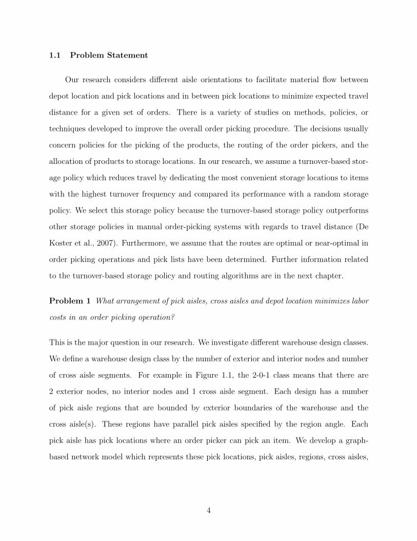
This is the major question in our research. We investigate different warehouse design classes.

We define a warehouse design class by the number of exterior and interior nodes and number

of cross aisle segments. For example in Figure 1.1, the 2-0-1 class means that there are

2 exterior nodes, no interior nodes and 1 cross aisle segment. Each design has a number

of pick aisle regions that are bounded by exterior boundaries of the warehouse and the

cross aisle(s). These regions have parallel pick aisles specified by the region angle. Each

pick aisle has pick locations where an order picker can pick an item. We develop a graph-

based network model which represents these pick locations, pick aisles, regions, cross aisles,

4

warehouse boundaries, and a depot location. Figure 1.2 shows an example of this graph-

based network model. Although, representation of a warehouse is an important part of the

answer to this question, we need to answer a related and a more difficult question.

Figure 1.1: Some warehouse design classes

Figure 1.2: A 3-0-2 class with a graph-based network model

Problem 2 How to measure the potential effectiveness of a design for a particular order

picking operation?

In an order picking operation, the number of picks and their locations may change for every

order picking tour. Compared to unit-load operations, where analytical models exist for

both traditional (Francis, 1967; Bassan et al., 1980) and non-traditional warehouses (Gue

and Meller, 2009; Ozturkoglu et al., 2014), there are no analytical models for more than

two cross aisles for order picking operations and the existing research has only focused on

traditional warehouse designs (Rosenblatt and Roll, 1984; De Koster et al., 2007). The

designs we develop in this research will not support an analytical model because of their

5

complex and stochastic nature. It is complex because solving each picking tour optimally is

a case of the traveling salesman problem (TSP), which has been solved optimally for one and

two block warehouses (Ratliff and Rosenthal, 1983; Roodbergen and De Koster, 2001b). It

is stochastic because evaluating only a single design is equivalent to solving hundreds of TSP

problems and evaluating a single tour would provide little information about the quality

of a design for an “expected order”. For these reasons, it is computationally hard to find

an optimal solution that minimizes the expected travel distance with a given order set and

design class.

Establishing efficient ways to evaluate designs, create more reasonable pick paths, and

search over solution space are three challenging computational problems. The first challenge

is mostly related to parallel and distributed computing techniques. Writing an efficient and

scalable parallel program is a complex task. However, C# parallel libraries provide the

power of parallel computing with simple changes in the implementation of finding a set of

optimal/near-optimal routes if a certain condition is met: the steps inside the operation

must be independent. Solving large batches of traveling salesman problems is an example of

such independent operations. In Chapter 3, we give details about the large batch of TSPs

and its solution techniques.

Even though warehouse design optimization has been studied since the early 1960s, all

design and routing techniques use a very common travel rule: workers follow the centers

of pick and cross aisles. But we propose the visibility graph method to address the second

challenge. The visibility graph method constructs a graph whose nodes are either vertices

of obstacles or attractions and whose edges are pairs of mutually visible nodes. In other

words, for any pair of nodes if the line segment that connects them does not pass through an

obstacle, an edge is created between them. Then we can run Dijkstra’s algorithm to find the

shortest path between any two nodes in this graph. In Chapter 4, we describe the visibility

graph method and compare it with the aisle centers method.

6

For the third challenge we propose Evolution Strategies (ES) as a heuristic optimizer.

ES is a meta-heuristic that works well with continuous problems. We present an encoding

that uses a string of continuous variables to define locations of the cross aisle endpoints, the

angles of picking aisles, and the location of the depot. Details of this algorithm and encoding

are given in Chapter 5.

Finally, we describe our design of experiments and its results in Chapter 6. We also

give a brief summary of the dissertation in this final chapter.

1.2 Major Contributions

Until Gue and Meller (2009) introduced the Flying-V and Fishbone layouts, the ware-

housing literature almost always assumed traditional warehouses (presented in Figure 4.4d)

and their slight variations. Ozturkoglu et al. (2014) extended this work by further relaxing

the established rules of warehouse design by using angled pick aisles. These designs resulted

in up to 22.52% savings over traditional unit-load warehouses. We are extending this existing

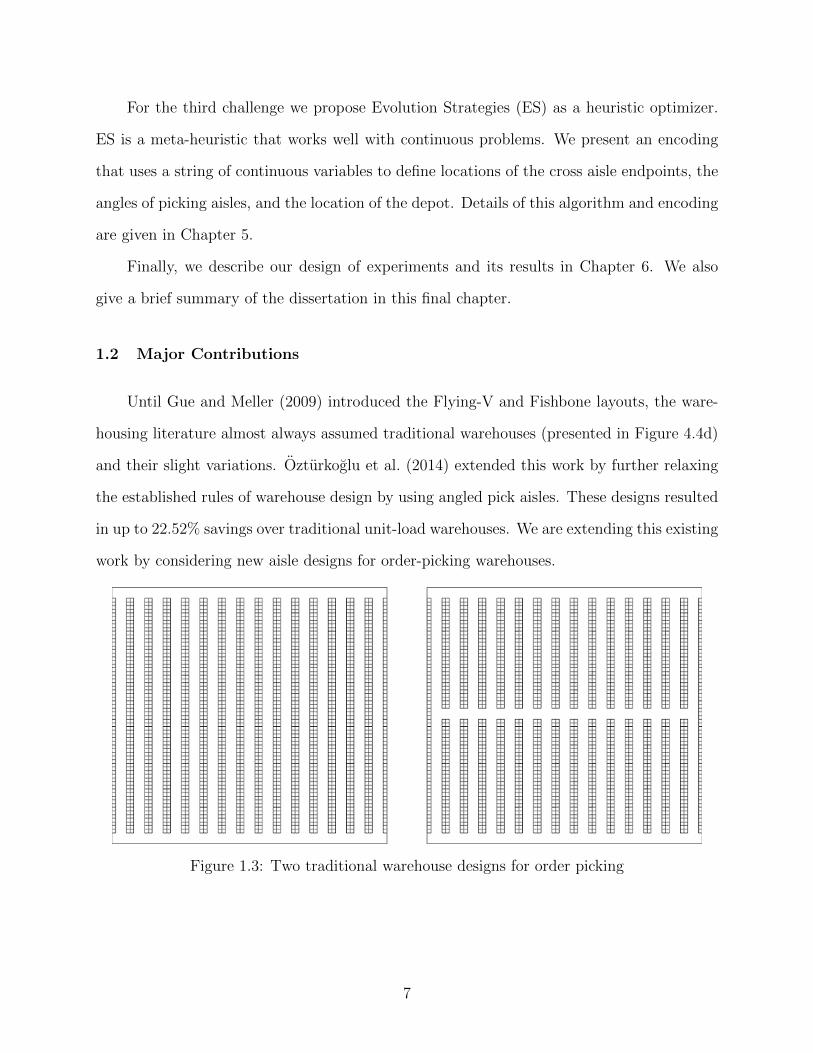
work by considering new aisle designs for order-picking warehouses.

Figure 1.3: Two traditional warehouse designs for order picking

7

Contribution 1 We develop near-optimal designs for different order-picking warehouse cat-

egories by searching through nineteen different warehouse design classes.

When we say order-picking warehouse category, we mean the order-picking warehouses that

show similar characteristics based on area, average number of stock keeping units (SKUs) ,

average number of units (such as pieces or cases that are less-than-unit load) per pick line,

etc. Frazelle (2002) describes different profiling techniques to characterize warehouses. We

relax traditional warehouse design assumptions and allow regions that have parallel pick

aisles inside their boundaries to take any angle and allow cross aisles to be oriented freely.

We also permit the depot location to float along a side of the warehouse and look for its

optimal location. However, we do not consider multiple depots in our research. With given

storage, routing and picking policy and set of orders, we propose to find optimal designs

by searching through nineteen different warehouse design classes: 0-0-0, 2-0-1, 2-1-2, 3-0-2,

3-0-3, 3-1-3, 3-1-4, 3-1-5, 3-1-6, 4-0-2, 4-0-3, 4-0-4, 4-0-5, 4-1-3, 4-1-4, 4-1-5, 4-1-6, 4-1-7, and

4-1-8 (see Figure 1.4).

We develop a graph-based network model that is used in the detailed evaluator function

of the two meta-heuristics, Particle Swarm Optimization (PSO) and ES. PSO and ES are

two meta-heuristics that work well with continuous problems. Ozturkoglu et al. (2014) used

PSO to find optimal angles for unit-load warehouses and this is the main reason for our PSO

selection. However, based on our experiments PSO did not perform well for the 2-0-1 design

class, therefore, we implemented ES. The comparison showed that ES performs better than

PSO for the 2-0-1 design class for unit-load operations with the randomized storage policy.

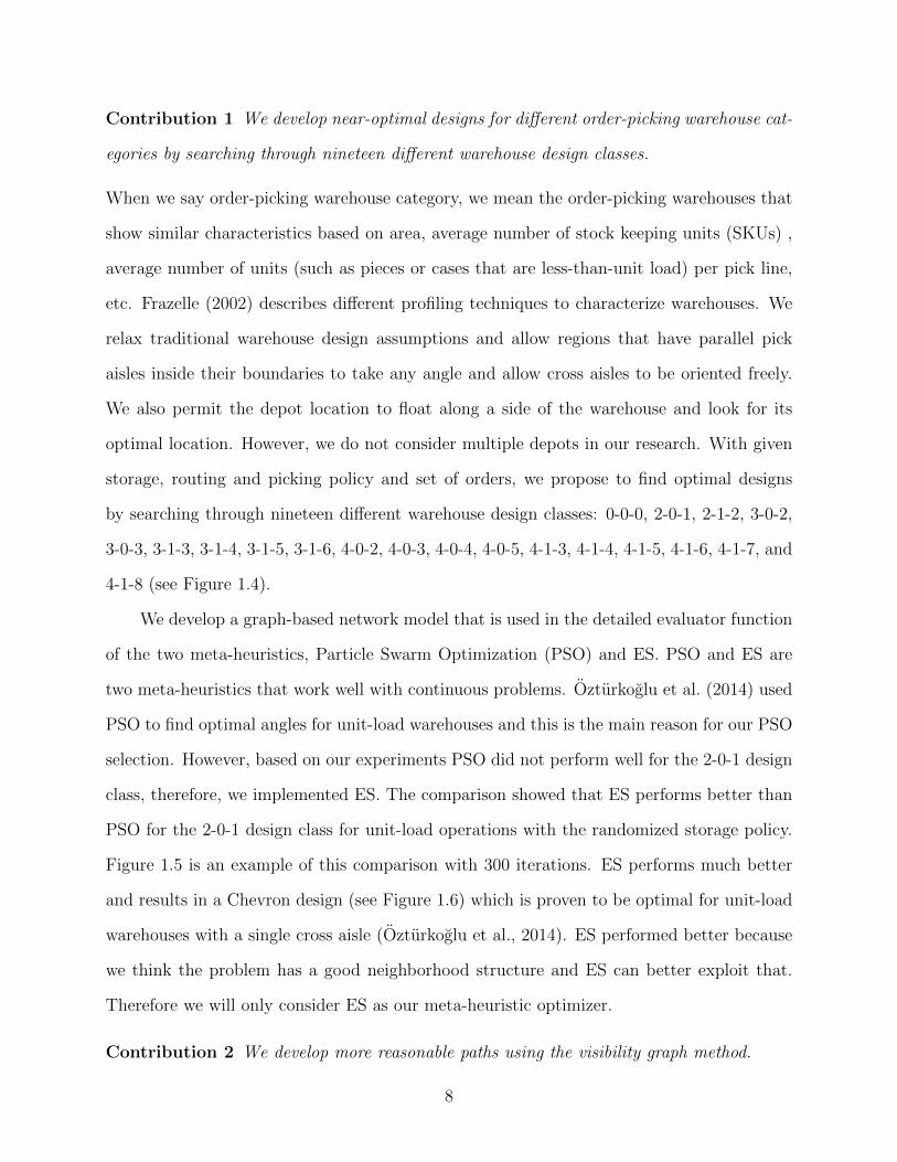
Figure 1.5 is an example of this comparison with 300 iterations. ES performs much better

and results in a Chevron design (see Figure 1.6) which is proven to be optimal for unit-load

warehouses with a single cross aisle (Ozturkoglu et al., 2014). ES performed better because

we think the problem has a good neighborhood structure and ES can better exploit that.

Therefore we will only consider ES as our meta-heuristic optimizer.

Contribution 2 We develop more reasonable paths using the visibility graph method.

8

(a) 0-0-0 (b) 2-0-1 (c) 2-1-2 (d) 3-0-2

(e) 3-0-3 (f) 3-1-3 (g) 3-1-4 (h) 3-1-5

(i) 3-1-6 (j) 4-0-2 (k) 4-0-3 (l) 4-0-4

(m) 4-0-5 (n) 4-1-3 (o) 4-1-4 (p) 4-1-5

(q) 4-1-6 (r) 4-1-7 (s) 4-1-8

Figure 1.4: Design classes that are being searched

9

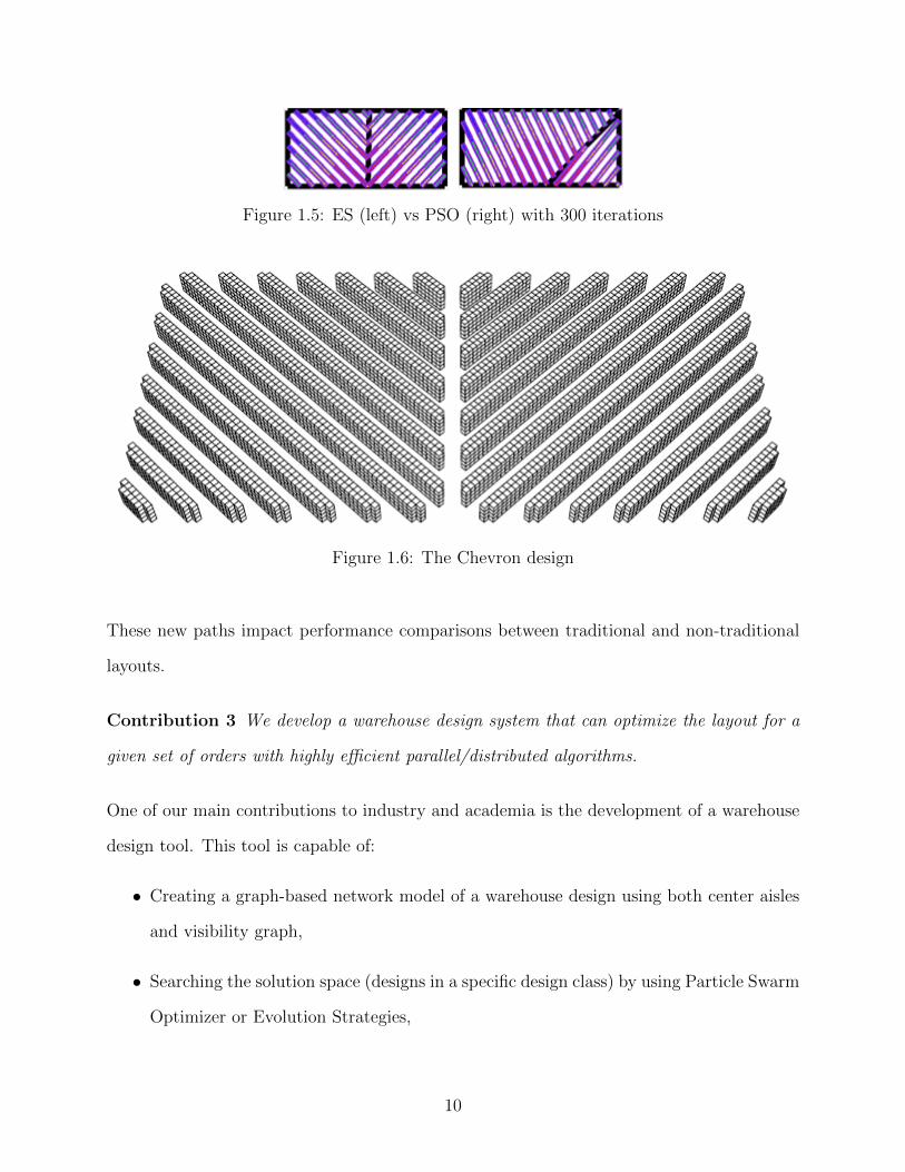
Figure 1.5: ES (left) vs PSO (right) with 300 iterations

Figure 1.6: The Chevron design

These new paths impact performance comparisons between traditional and non-traditional

layouts.

Contribution 3 We develop a warehouse design system that can optimize the layout for a

given set of orders with highly efficient parallel/distributed algorithms.

One of our main contributions to industry and academia is the development of a warehouse

design tool. This tool is capable of:

• Creating a graph-based network model of a warehouse design using both center aisles

and visibility graph,

• Searching the solution space (designs in a specific design class) by using Particle Swarm

Optimizer or Evolution Strategies,

10

• Showing a graphical representation of the warehouse with cross and pick aisles, and

pick locations,

• Showing the most and the least convenient storage locations in different colors,

• Interfacing with TSP Solver Concorde and Lin-Kernighan-Helsgaun to find the optimal/near-

optimal routing per pick tour,

• Importing order pick list data in order to allocate products and to perform design

optimization,

• Importing a list of different warehouse designs in Excel format to calculate their ob-

jective functions and export the list of designs with their objective function values.

This capability is helpful to someone who wants to create a design of experiments to

perform regression or use it as a training data set for ANNs or another meta-modeling

technique,

• Searching nineteen different warehouse design classes,

• Calculating the wasted space used by cross aisles,

• Solving large batches of TSPs in parallel and distributed computing environments.

11

Chapter 2

Literature Review

2.1 Warehouse Operations

A warehouse is defined as a place for storing or buffering large quantities of raw ma-

terials, work-in-process items or finished goods. Warehouses are used by manufacturers,

wholesalers, importers, exporters, etc. Figure 2.1 shows the functional areas and operations

within warehouses. In a typical warehouse, items are received from suppliers, they are stored

in storage locations, order pickers fulfill customer orders and assemble them for shipment,

and completed orders are shipped to customers. A typical warehouse shares many functions

with a cross-docking warehouse. However, storage is an important function in a typical

warehouse, while in a cross-docking warehouse, there is little or no storage (Bartholdi and

Hackman, 2011).

Figure 2.1: Typical warehouse flows and operations (Tompkins, 2010)

12

2.1.1 Receiving and Shipping

Receiving is the first activity in a warehouse. When an inbound trucker phones the

warehouse to get a delivery appointment, the receiving operation begins. The trucker arrives

at the assigned receiving dock, goods are unloaded and inspected at a place before being

stored in an assigned location. This place is called the “pickup and deposit (P&D) point”.

For cross-docking warehouses, received items are sent directly from the receiving docks to

the shipping docks. For typical warehouses, received items are put into storage. Then orders

are picked from storage, prepared for shipment, and shipped to customers through shipping

docks. The receiving and shipping operations are integrated with the storage and order

picking operations and this makes the receiving and shipping operations more complicated

in typical warehouses than in cross-docking warehouses (Gu et al., 2007). The literature on

receiving and shipping is very limited and has been focused on the truck-to-dock assignment

problem for cross-docking warehouses (see Gu et al. (2007), for details).

2.1.2 Storage

Storage is the physical containment of an item while it is awaiting a demand (Tompkins,

2010). According to Bartholdi and Hackman (2011), a storage mode means a region of

storage or a piece of equipment for which the costs to pick/restock from any location are all

approximately equal. The storage mode of items depends on the size and quantity of the

items in inventory and the handling characteristics of the product or its container. Storage

modes can be grouped into two main categories: storage modes for unit-load operations and

storage modes for less-than-unit-load operations. A unit-load combines individual items or

items in shipping containers into single units that can be moved easily with a pallet jack or

forklift truck. The typical unit-load is a pallet. Pallets are either stored in block stacking

or pallet racks (and their slight variations). Because pallets are (mostly) standardized and

are generally large, they are mostly handled one at a time in unit-load operations. Third-

party transshipment warehouses are typically unit-load warehouses that receive, store, and

13

forward pallets. Many warehouses also perform unit-load operations in some portion of their

activities. Storage modes for less-than-unit-load storage include items that are generally

stored in cases or cartons (and sometimes pieces). The most popular less-than-unit-load

storage mode systems are bin shelving, modular storage drawers/cabinets, and gravity flow

racks (Frazelle, 2002). Selection of storage mode generally includes these objectives:

• Efficient space use,

• Efficient material handling,

• The most economical storage in relation to costs of equipment use of space, damage of

material, handling labor, and operational safety,

• Maximum flexibility in order to meet changing storage and handling requirements, and

• A good model of the organization of SKUs throughout the warehouse.

Detailed literature about storage mode selection is in Frazelle (2002) and Bartholdi and

Hackman (2011).

When the storage mode is selected for each item, a decision must be made for storage

assignment for each item. The product allocation problem concerns the assignment of items

to storage locations. There are five frequently used product allocation policies: random

storage, closest-open location storage, class-based storage, full-turnover storage, and dedi-

cated storage (De Koster et al., 2007). Random storage, closest-open location storage, and

class-based storage are also called shared storage.

The random storage policy allows items to be stored anywhere in the storage area

with equal probability. This policy has an advantage of higher space utilization (or low

space requirement) at the expense of increased travel distance (Choe and Sharp, 1991),

but it is harder to manage, because locations of items change over time. The closest-open

location storage policy allows order pickers to choose the location for storage themselves.

This policy leads to a storage area where storage locations are full around the depot location

14

and gradually empty towards the back. The class-based storage policy distributes the items

based on some measure of demand frequency, among a number of classes, where each class

represents a region within the storage area. The idea is based on Pareto’s method: 85% of the

turnover will be a result of 15% of the items stored. To increase the order picking efficiency,

the most popular 15% of items should be stored such that travel distance is minimized.

Storage within a region is random.

The full-turnover storage policy distributes items over the storage area according to

their turnover. Items with the highest turnover rates are stored at the“closer to depot”

locations or “easily accessible” locations. Slow moving items are stored closer to the back of

the storage area. The dedicated storage policy assigns each product to a specific location.

Material handling workers know in advance where to store items and order pickers become

familiar with the locations of items which reduces time wasted for searching. On the other

hand, average storage capacity is only about 50% utilized (Bartholdi and Hackman, 2011).

Petersen and Aase (2004) show that with regard to travel distance in a manual order-picking

system, full-turnover storage and class-based storage outperform random storage. However,

these policies may also increase picker congestion within aisles containing the most popular

SKUs. Also, they may require periodic movement of SKUs because of demand seasonality

of SKUs. Cube-per-order index (COI) is one of the most well known implementations of the

full turnover-based storage policy (Heskett, 1963, 1964). The COI of a product is the ratio

of the product’s total required space to the number of trips required to satisfy its demand

per period. The ones with the lowest COI are located closest to the depot. Goetschalckx

and Ratliff (1990) consider shared storage and show that a duration-of-stay policy is optimal

under an assumption of perfectly balanced inputs and outputs. The duration-of-stay policy

requires arrival/departure information on individual items of a particular product, whereas

the turnover-based and class-based storage policies require only turnover rate information

at the product level. In this research we assume we know only product information.

15

Each storage policy has advantages and disadvantages. Some disadvantages can be

easily eliminated by using a warehouse management system (WMS) that gives information

to material handling workers and reduces search and travel time. But this may not be

the case in practice. According to Bartholdi and Hackman (2011), shared storage requires

greater software support and more disciplined warehouse processes. For example, a worker

might pick the item from a more convenient location rather than a farther location that is

given by the WMS.

2.1.3 Order Picking

Order picking is the retrieval of items from a storage area to fulfill customer orders. It

involves the process of grouping and scheduling customer orders, releasing them to the order

pickers, the picking of the items from storage locations, and the disposal of the picked items

(De Koster et al., 2007). The main objective of order picking is to maximize the service

level subject to resource constraints such as labor, machines, and capital (Goetschalckx and

Ashayeri, 1989). The faster an order can be retrieved, the sooner it is available for shipping

to the customer. If the warehouse cannot process orders quickly, effectively, and accurately

then service level optimization efforts will suffer. Any inefficiency in order picking can lead

some orders to miss their shipping due time. These orders either have to wait until the next

shipping period or have to be shipped with expedited shipping. Either way, the warehouse

will suffer from customer dissatisfaction or additional cost. Therefore, minimizing order

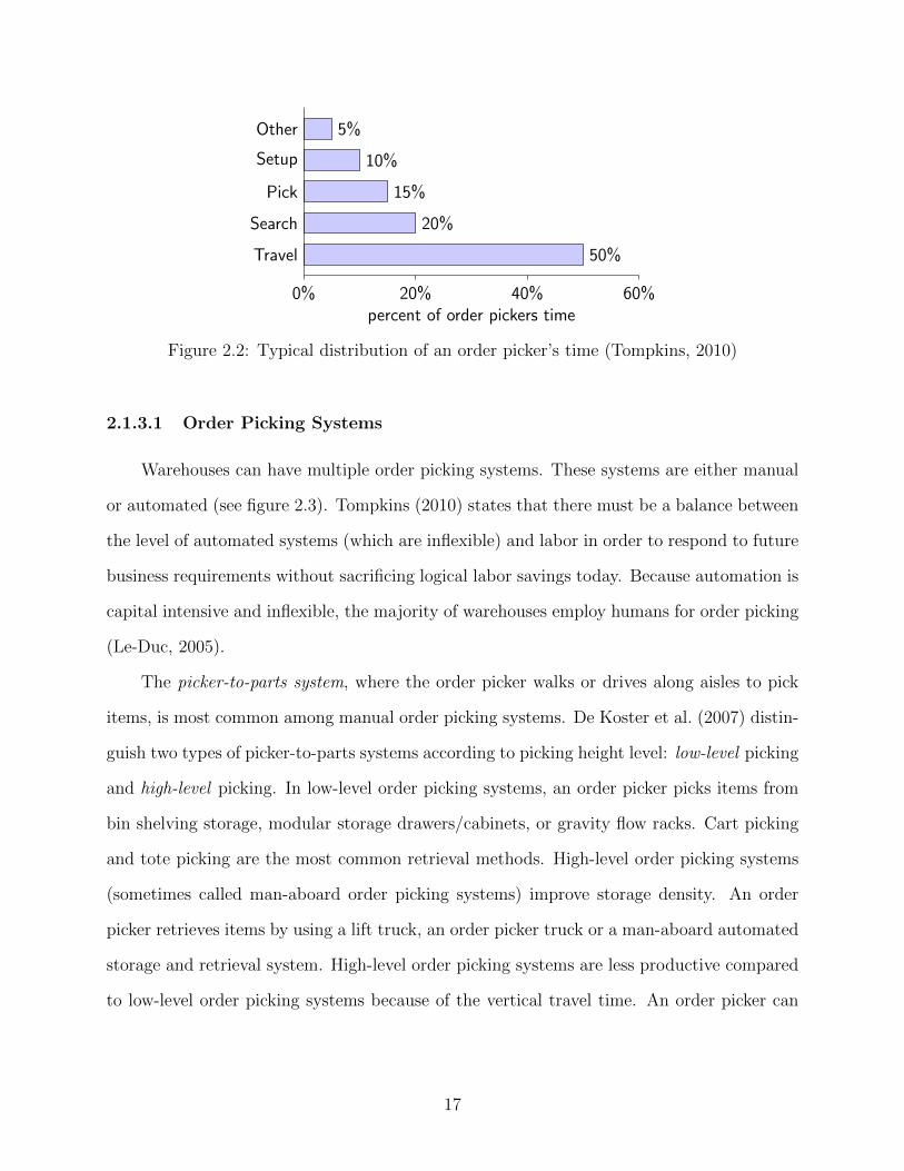
retrieval time is a key to a successful warehouse. Figure 5.1 shows the order picking time

components in a typical warehouse. 50% of the order picker’s time is travel time. Travel time

is a direct expense but it does not add value, therefore it is a waste (Bartholdi and Hackman,

2011). For manual-pick order picking systems, the travel time is an increasing function of

the travel distance (De Koster et al., 2007). For these reasons, we select minimizing travel

distance as an objective for improvement.

16

5%Other

10%Setup

15%Pick

20%Search

50%Travel

0% 20% 40% 60%percent of order pickers time

Figure 2.2: Typical distribution of an order picker’s time (Tompkins, 2010)

2.1.3.1 Order Picking Systems

Warehouses can have multiple order picking systems. These systems are either manual

or automated (see figure 2.3). Tompkins (2010) states that there must be a balance between

the level of automated systems (which are inflexible) and labor in order to respond to future

business requirements without sacrificing logical labor savings today. Because automation is

capital intensive and inflexible, the majority of warehouses employ humans for order picking

(Le-Duc, 2005).

The picker-to-parts system, where the order picker walks or drives along aisles to pick

items, is most common among manual order picking systems. De Koster et al. (2007) distin-

guish two types of picker-to-parts systems according to picking height level: low-level picking

and high-level picking. In low-level order picking systems, an order picker picks items from

bin shelving storage, modular storage drawers/cabinets, or gravity flow racks. Cart picking

and tote picking are the most common retrieval methods. High-level order picking systems

(sometimes called man-aboard order picking systems) improve storage density. An order

picker retrieves items by using a lift truck, an order picker truck or a man-aboard automated

storage and retrieval system. High-level order picking systems are less productive compared

to low-level order picking systems because of the vertical travel time. An order picker can

17

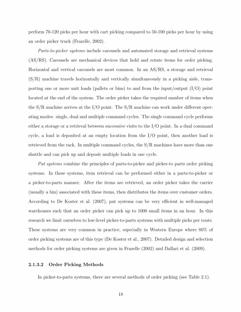
perform 70-120 picks per hour with cart picking compared to 50-100 picks per hour by using

an order picker truck (Frazelle, 2002).

Parts-to-picker systems include carousels and automated storage and retrieval systems

(AS/RS). Carousels are mechanical devices that hold and rotate items for order picking.

Horizontal and vertical carousels are most common. In an AS/RS, a storage and retrieval

(S/R) machine travels horizontally and vertically simultaneously in a picking aisle, trans-

porting one or more unit loads (pallets or bins) to and from the input/output (I/O) point

located at the end of the system. The order picker takes the required number of items when

the S/R machine arrives at the I/O point. The S/R machine can work under different oper-

ating modes: single, dual and multiple command cycles. The single command cycle performs

either a storage or a retrieval between successive visits to the I/O point. In a dual command

cycle, a load is deposited at an empty location from the I/O point, then another load is

retrieved from the rack. In multiple command cycles, the S/R machines have more than one

shuttle and can pick up and deposit multiple loads in one cycle.

Put systems combine the principles of parts-to-picker and picker-to parts order picking

systems. In these systems, item retrieval can be performed either in a parts-to-picker or

a picker-to-parts manner. After the items are retrieved, an order picker takes the carrier

(usually a bin) associated with these items, then distributes the items over customer orders.

According to De Koster et al. (2007), put systems can be very efficient in well-managed

warehouses such that an order picker can pick up to 1000 small items in an hour. In this

research we limit ourselves to low-level picker-to-parts systems with multiple picks per route.

These systems are very common in practice, especially in Western Europe where 80% of

order picking systems are of this type (De Koster et al., 2007). Detailed design and selection

methods for order picking systems are given in Frazelle (2002) and Dallari et al. (2009).

2.1.3.2 Order Picking Methods

In picker-to-parts systems, there are several methods of order picking (see Table 2.1).

18

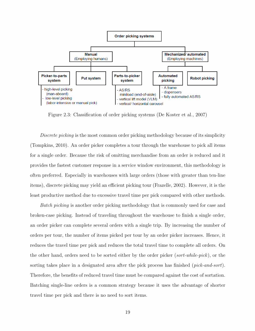
Figure 2.3: Classification of order picking systems (De Koster et al., 2007)

Discrete picking is the most common order picking methodology because of its simplicity

(Tompkins, 2010). An order picker completes a tour through the warehouse to pick all items

for a single order. Because the risk of omitting merchandise from an order is reduced and it

provides the fastest customer response in a service window environment, this methodology is

often preferred. Especially in warehouses with large orders (those with greater than ten-line

items), discrete picking may yield an efficient picking tour (Frazelle, 2002). However, it is the

least productive method due to excessive travel time per pick compared with other methods.

Batch picking is another order picking methodology that is commonly used for case and

broken-case picking. Instead of traveling throughout the warehouse to finish a single order,

an order picker can complete several orders with a single trip. By increasing the number of

orders per tour, the number of items picked per tour by an order picker increases. Hence, it

reduces the travel time per pick and reduces the total travel time to complete all orders. On

the other hand, orders need to be sorted either by the order picker (sort-while-pick), or the

sorting takes place in a designated area after the pick process has finished (pick-and-sort).

Therefore, the benefits of reduced travel time must be compared against the cost of sortation.

Batching single-line orders is a common strategy because it uses the advantage of shorter

travel time per pick and there is no need to sort items.

19

Zone picking divides the order picking area into distinct sections and assigns order

pickers to picking zones. Picking zones should not be mistaken for storage zones, which are

defined to facilitate efficient and safe storage and are specified in slotting. In zone picking, an

order picker works on one order at a time and picks all lines that are located within that zone

for that order. Then, these items are brought to an area for consolidation before shipment.

Traversal of a smaller area, reduced traffic congestion, good housekeeping in the order picker’s

zone (items are better organized in picking zone), and the order pickers’ familiarity with the

item locations are the main advantages of zoning. The main disadvantages of zoning are the

cost of sorting and the potential for order-filling errors. Zoning might be necessary because

of the different skills or equipment associated with a warehouse. Also product properties

such as size, weight, and safety requirements might force a warehouse manager to define

zones in the warehouse.

There are two variations for establishing order integrity in zone picking. Sequential zone

picking (or progressive zoning) is picking one zone at a time, then passing the order to next

zone until the order is completed. The contents of the order generally move in a tote and the

order picker hands the tote and pick list to the next picker. Some intelligent systems may

skip zones where no items need to be picked (zone skipping). In simultaneous zone picking

(or synchronized zoning), a number of order pickers within their zones start on the same

order in parallel, then these partial orders are consolidated at a designated location. Wave

picking is same as discrete picking except that a selected group of orders is scheduled to be

picked during a specific time horizon. The other three methodologies are combinations of the

methodologies described above, therefore they are more complex and require more control.

2.1.3.3 Routing Methods

Routing methods determine the picking sequence of items on the pick list to ensure a

good route through the warehouse. The problem of sequencing and routing order pickers is

a special case of the TSP, classified as the Steiner TSP. In a classical TSP, given distances

20

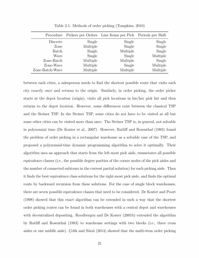
Table 2.1: Methods of order picking (Tompkins, 2010)

Procedure Pickers per Orders Line Items per Pick Periods per Shift

Discrete Single Single SingleZone Multiple Single Single

Batch Single Multiple SingleWave Single Single Multiple

Zone-Batch Multiple Multiple SingleZone-Wave Multiple Single Multiple

Zone-Batch-Wave Multiple Multiple Multiple

between each cities, a salesperson needs to find the shortest possible route that visits each

city exactly once and returns to the origin. Similarly, in order picking, the order picker

starts at the depot location (origin), visits all pick locations in his/her pick list and then

returns to the depot location. However, some differences exist between the classical TSP

and the Steiner TSP. In the Steiner TSP, some cities do not have to be visited at all but

some other cities can be visited more than once. The Steiner TSP is, in general, not solvable

in polynomial time (De Koster et al., 2007). However, Ratliff and Rosenthal (1983) found

the problem of order picking in a rectangular warehouse as a solvable case of the TSP, and

proposed a polynomial-time dynamic programming algorithm to solve it optimally. Their

algorithm uses an approach that starts from the left-most pick aisle, enumerates all possible

equivalence classes (i.e., the possible degree parities of the corner nodes of the pick aisles and

the number of connected subtours in the current partial solution) for each picking aisle. Then

it finds the best equivalence class solutions for the right-most pick aisle, and finds the optimal

route by backward recursion from these solutions. For the case of single block warehouses,

there are seven possible equivalence classes that need to be considered. De Koster and Poort

(1998) showed that this exact algorithm can be extended in such a way that the shortest

order picking routes can be found in both warehouses with a central depot and warehouses

with decentralized depositing. Roodbergen and De Koster (2001b) extended the algorithm

by Ratliff and Rosenthal (1983) to warehouse settings with two blocks (i.e., three cross

aisles or one middle aisle). Celik and Sural (2014) showed that the multi-item order picking

21

problem can be solved in polynomial time for both fishbone and flying-V layouts. The main

idea behind their algorithm is to transform the fishbone layout into an equivalent warehouse

setting with two blocks. For warehouses with three or more blocks, the number of possible

equivalence classes increases exponentially (Celik and Sural, 2014). Therefore, extending the

algorithm is of little of use.

The existing literature has largely been devoted to finding efficient heuristics because

efficient optimal algorithms are not available for every layout, and optimal routes may not

consider real-world problems in order picking such as aisle congestion. For example, an

S-shape can avoid aisle congestion because it has a single direction if the pick density is

sufficiently high (i.e., there is at least one pick in every aisle). Many routing policies described

in the literature have been analyzed for four types of warehouse systems (i.e., conventional

multi-parallel-aisle systems, man-on-board AS/RS, unit-load AS/RS, and carousel systems)

(Gu et al., 2007). When using a S-shape heuristic, order pickers must completely traverse

the entire aisle containing at least one pick. Aisles without picks are not visited. From

the last entered aisle, the order picker returns to the depot. In the return method, the

order picker enters and leaves each aisle from the same end and only visits aisles with picks.

The midpoint policy divides the warehouse into two areas (see Figure 2.4). The heuristic

collects all the items in the upper section, after which the lower section is dealt with. In the

largest gap method, the order picker traverses the first and last aisle with picks entirely. All

the other aisles are entered from the front and back in such a way that the non-traversed

distance between two adjacent locations of items to be picked in the aisle is maximized. In

the composite heuristic, aisles with picks are visited, but dynamic programming is used to

decide either entirely traverse or enter and left at the same end (see Roodbergen and De

Koster (2001a)). Petersen (1997) analyzed six routing heuristics (S-shape, return, midpoint,

largest gap, composite, and optimal) for single-block warehouses and concluded that the best

heuristic solution is on average 5% more than the optimal solution (see Figure 2.4).

22

These routing heuristics are not suitable for our research for two reasons. First, these

heuristics are designed for single-block warehouses and some (aisle-by-aisle, S-shape, largest

gap, combined) can be modified for multiple-block warehouses, but they are not designed

for non-traditional designs. Therefore, the routing might not work in some non-traditional

designs. Second and most important, these heuristics are fairly simple construction heuristics

which construct a feasible solution, without attempting any improvement by means of local

search or meta-heuristic search.

Makris and Giakoumakis (2003) present Lin and Kernighan (1973)s TSP-based k-

interchange methodology for single-block warehouses and show that their procedure out-

performed the S-shape heuristic in seven of eleven examined cases. Theys et al. (2010)

extended their research for multi-block warehouses and achieved average savings in route

distance of up to 47% when using the Lin-Kerhighan-Helsgaun (LKH) heuristic (Helsgaun,

2000) compared to S-shape, largest gap, combined, and aisle-by-aisle heuristics. The quality

of the solutions by the LKH heuristic is, on average, clearly superior to the other routing

heuristics. Although the LKH heuristic’s average computation time (0.25 seconds) is more

than these heuristics (the calculation time is negligible for these heuristics) it is 36 times

faster than the exact TSP algorithm “Concorde” (9.23 seconds). Moreover, LKH’s solutions

deviate on average only 0.1% from optimum. A detailed description of these routing policies

and their variations can be found in De Koster et al. (2007), Gu et al. (2007), and Helsgaun

(2000).

2.1.3.4 Complexity of Order Picking Systems

Figure 2.5 helps us to identify the complexity of order picking systems. If the system is

further from the origin, it is harder to design and manage. In our research we are focused

on manual, static, many aisles, continuous, no-zoning, pick-by-order order picking systems.

We are interested only in turnover-based storage policy, because it outperforms random and

class-based storage policies with regards to travel distance (Petersen and Aase, 2004). We

23

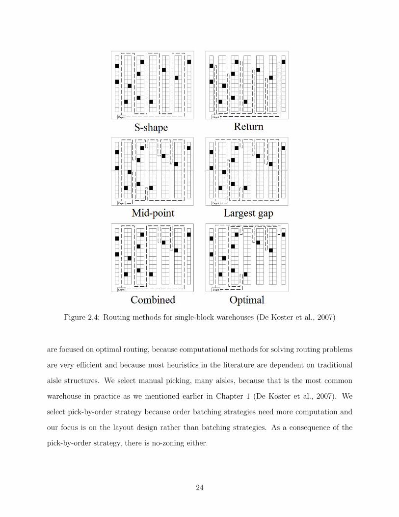
Figure 2.4: Routing methods for single-block warehouses (De Koster et al., 2007)

are focused on optimal routing, because computational methods for solving routing problems

are very efficient and because most heuristics in the literature are dependent on traditional

aisle structures. We select manual picking, many aisles, because that is the most common

warehouse in practice as we mentioned earlier in Chapter 1 (De Koster et al., 2007). We

select pick-by-order strategy because order batching strategies need more computation and

our focus is on the layout design rather than batching strategies. As a consequence of the

pick-by-order strategy, there is no-zoning either.

24

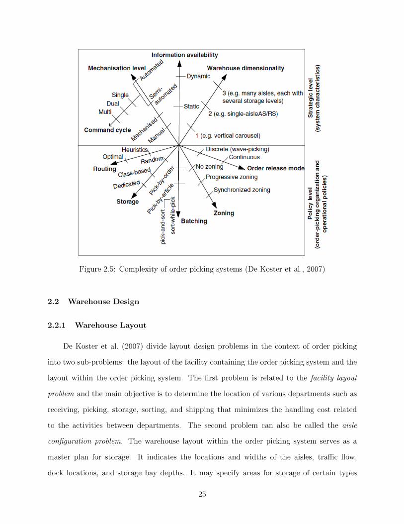
Figure 2.5: Complexity of order picking systems (De Koster et al., 2007)

2.2 Warehouse Design

2.2.1 Warehouse Layout

De Koster et al. (2007) divide layout design problems in the context of order picking

into two sub-problems: the layout of the facility containing the order picking system and the

layout within the order picking system. The first problem is related to the facility layout

problem and the main objective is to determine the location of various departments such as

receiving, picking, storage, sorting, and shipping that minimizes the handling cost related

to the activities between departments. The second problem can also be called the aisle

configuration problem. The warehouse layout within the order picking system serves as a

master plan for storage. It indicates the locations and widths of the aisles, traffic flow,

dock locations, and storage bay depths. It may specify areas for storage of certain types

25

of products. The layout may also include specialized areas for order picking, high security

storage, or temperature controlled space. Space is often lost because of the need for access

to each item on the pick list (honeycombing), and this loss can be minimized by an effective

layout (Ackerman et al., 1972). The most common objective function is travel distance (De

Koster et al., 2007). Our research focuses on this second sub-problem.

The literature related to the aisle configuration problem is mostly related to traditional

warehouses. Several researchers used different combinations of P&D locations. Bassan et al.

(1980) showed that the depot should be centrally located under the condition of random

storage to minimize average travel distance. Kunder and Gudehus (1975) and Hall (1993)

considered a centrally located P&D location and derive analytical travel models for manual

order-picking. Bartholdi and Hackman (2011) divide the layout problem within the order

picking system into three types: layout of a unit-load area, layout of a carton-pick-from pallet

area, and layout of a piece-pick-from-carton area.

A unit-load warehouse means that only a single unit (typically a pallet) of material

is handled at a time. It is the simplest type of warehouse. Third party warehouses and

import warehouses are examples of unit-load warehouses that receive, store and ship pallets.

Many warehouses also devote some portion of their activity to unit-load operations. In

single-command operations, one item is picked or stored during one trip by an operator.

Hence, operators travel empty either when they return to a P&D location or go to a storage

location for picking (dead-heading). Single-command operations are common in unit-load

warehouses and unit-load replenishment in the reserve area. Francis (1967) and Bassan et al.

(1980) modeled single-command travel distance in traditional warehouses and present some

well-known results on optimal warehouse shape and P&D location. In order to reduce dead-

heading, dual-command operations can be used. In dual-command operations, an operator

deposits an item and then goes to another location to pick another item, then returns back

to a P&D location. Malmborg and Bhaskaran (1987) considered dual-command travel in

traditional warehouses. Pohl et al. (2009a) develop expected travel distance equations in

26

traditional designs with a middle cross aisle for dual-command operations. The literature

on the layout design problem for unit-load warehouses has mainly focused on AS/RS (see

Sarker and Babu (1995) and Roodbergen and Vis (2009) for extended literature reviews on

AS/RS).

The second type of layout problem is carton-pick-from-pallet-area where the storage

or restocking operation is done by pallets but the picking is done with cartons or cases,

which makes it different than unit-load warehouses. The handling unit (a carton or case)

weighs between 5 and 50 pounds and the picking operation can be handled by one person.

The warehouse is divided into two areas: forward area and reserve area. Popular SKUs are

usually placed in the forward area for case-picking and replenished from the reserve area.

The problem of deciding which products should be stored in the forward area and in what

quantities is called the forward-reserve problem (FRP). If a product is not stored in the

forward area, then it needs to be picked from the reserve area. The most common pick

area is the ground floor of a pallet rack. Generally, dedicated storage is used in the forward

area. Hackman et al. (1990) presented a heuristic method for the FRP that attempts to

minimize the total costs for picking and replenishing. Frazelle et al. (1994) extended their

work to determine the size of the forward area together with the allocated products. Van

den Berg et al. (1998) considered busy and idle periods for order picking operations to find

an allocation of product quantities in the forward area which minimizes the expected labor

time during the picking period. Reducing the number of replenishments in busy periods

by performing replenishments in idle periods not only increases throughput during the busy

periods but also reduces possible congestion. Gu (2005) proposes a bi-level hierarchical

heuristic approach that is very efficient in generating near optimal solutions for sizing and

dimensioning of a forward-reserve warehouse.

A third type of layout problem is piece-pick-from-carton-area where storing or restocking

operations are done by cartons but the picking operation is done with pieces. It is the most

labor intensive activity in the warehouse because the product is handled at the smallest

27

unit-of-measure. Moreover, the importance of piece-picking operation has increased in the

past 20 years because of pressure to reduce inventory and use the remaining space to expand

product variety. A general rule of thumb in this type of warehouse is to separate the storage

and the picking activities. A fast-pick area is a sub-region of the warehouse in which picks

and orders are concentrated within a small physical space. This leads to reduced pick costs

and quick response to customer demand.

2.2.2 Non-Traditional Designs

There has been much work done in the literature related to order picking warehouses

and how to modify their designs. However, most previous research assumed two design rules:

• Picking aisles must be straight and parallel to each other.

• If present, cross aisles must be straight, parallel to each other and orthogonal to the

picking aisles.

In the late 2000s, the non-traditional warehouse layout problem became a main focus.

Gue and Meller (2009) proposed two non-traditional unit-load aisle configurations: the flying-

V and fishbone layouts (see Figure 2.6). The former has two nonlinear cross aisles inserted

into a traditional layout and offers about 10% improvement over the traditional design.

The latter has two angled cross aisles at 45◦ and 135◦, with picking aisles at 0◦, 90◦, and

180◦ in the regions divided by the angled cross aisles and offers about 20% improvement

over the traditional design. Pohl et al. (2009b) modeled a dual-command expected travel

distance expression for the fishbone layout and observed that the fishbone design still reduces

dual-command travel by approximately 10%-15%. They also offered a fishbone-triangle

for dual-command operations by inserting an additional cross aisle segment between two

diagonal cross aisles for dual-command operations. Ozturkoglu et al. (2014) extended the

work by Gue and Meller (2009) to the case of angled picking aisles. They showed that up to

28

22.52% reduction in single-command travel distance is possible, as compared to a traditional

warehouse with parallel aisles.

(a) Flying-V (b) Fishbone

Figure 2.6: Flying-V and Fishbone layouts proposed by Gue and Meller (2009)

To the best of our knowledge, there exists only a few studies that discuss the performance

of the fishbone layout under multiple-item picks. Dukic and Opetuk (2008) analyzed the

fishbone layout and concluded that it results in larger routes than the traditional layout

under multiple-item picks. However, their analysis is based on the results of an S-shape

heuristic modified for fishbone layout and they only considered a random storage policy. Celik

and Sural (2014) filled the gap by presenting a polynomial-time algorithm that optimally

solves the picker routing problem and presented alternative heuristic methods. They also

presented their analyses for different warehouse sizes and shapes, and under random and

turnover-based storage policies. They showed that as the size of the pick list grows, the

fishbone is outperformed by the traditional layout under random storage, with a maximum

gap of around 36%. They observed that the relative performance of the fishbone layout is

better under random demand for single-command operations, whereas it performs better

under more skewed demand when the pick list size grows larger.

29

2.3 Heuristic Optimization

2.3.1 Particle Swarm Optimization

Particle swarm optimization (PSO) is one of the most popular evolutionary algorithms.

It was introduced by Kennedy and Eberhart (1995) as an alternative to other evolutionary

algorithms, such as genetic algorithms, evolution strategies, and differential evolution to

solve continuous non-linear functions. The paradigm is inspired by the flocking of birds and

schooling of fish.

In the original PSO algorithm, each particle represents a solution that moves toward

its previous best position and the global best position found in the population so far. After

initializing parameters and generating the initial population randomly, each particle is eval-

uated by the fitness function. After evaluation, each particle updates its position, velocity,

and fitness value. If there is an improvement in its fitness value, it updates its personal best.

If the best particle in the population improves the global best (i.e., the best particle found so

far in the population), then the global best is also updated. Next, the velocity of the particle

is updated by using its previous velocity, personal best and the global best to move the par-

ticle to another (hopefully, better) place in the search space. The algorithm performs these

steps repeatedly until it is terminated by a stopping criterion such as maximum number of

iterations. Shi and Eberhart (1998a,b) introduced an inertia weight to the algorithm. It is

denoted as w and is used to balance global and local search. It can be a positive constant or

a function of iteration. A larger w means that higher importance is given to global search,

while smaller values of w favors local search. Some application areas of PSO are chemistry

and chemical engineering (Cedeno and Agrafiotis, 2003; Shen et al., 2004), function opti-

mization (Kennedy and Eberhart, 1995; Parsopulos and Vrahatis, 2002), operations research

(Baltar and Fontane, 2006), and machine learning (Meissner et al., 2006).

Several studies have been done related to warehouse layout optimization using PSO

(Onut et al., 2008; Sooksaksun et al., 2012; Ozturkoglu et al., 2014). However, research

30

focusing on warehouse design optimization using PSO has been either focused on order pick-

ing operations for traditional warehouse layouts or unit-load operations for non-traditional

layout designs. To the best of our knowledge, there is a lack of research combining these two

aspects.

2.3.2 Evolution Strategies

Evolution strategies (ES) were introduced by Rechenberg (1965) and Schwefel (1965)

and imitate the principles of natural evolution as a method to solve parameter optimiza-

tion problems. ES is a population-based meta-heuristic optimization algorithm that uses

biology-inspired mechanisms such as mutation, crossover, and survival of the fittest in or-

der to refine a set of solution candidates iteratively. The advantage of ES compared to

other optimization methods is its “black box” character that makes only few assumptions

about the underlying objective functions. Moreover, objective function definitions generally

require less insight into the structure of the problem space than the manual construction

of an admissible heuristic. Therefore, the performance of ESs is generally good for many

problem classes. Some application areas of ES are data mining and data analysis (Cordon

et al., 1998), scheduling (Huang et al., 1999), chemistry and chemical engineering (Roosen

and Meyer, 1992; Cutello et al., 2005; Emmerich et al., 2000), resource minimization and

environment surveillance/protection (O’Brien et al., 2003), combinatorial optimization (Nis-

sen and Krause, 1994; Beyer, 1992), geometry and physics (Keller et al., 1999; Weinert and

Mehnen, 2001), and optics and image processing (Greiner, 1996; Back and Schutz, 1995;

Wiesmann et al., 1998; Li et al., 2006). There are several variants of ES based on popu-

lation strategy. The (1+1)-ES consists of a single individual which is reproduced. Both

the elder and the offspring compete and the better individual survives to form the next

population. The (1,1)-ES is equivalent to random walk because in every generation the

parent is replaced with its offspring and there is no survival of the fittest. The (µ + 1)-ES

contains µ individuals from which one is drawn randomly. This individual is reproduced

31

from the current population, and the worst fit individual is removed from the the joint set

of its offspring and the current population. This strategy is also called “Elimination of the

worst”. The (µ + λ)-ES uses reproduction operations and from µ parent individuals λ ≥ µ

offspring are created. From the joint set of parents and offspring, only the µ fittest ones

survive (Schwefel, 1975, 1977). In (µ, λ)-ES, introduced by Schwefel (1981), λ ≥ µ offspring

are created from µ parents. The parents are subsequently replaced with the µ fittest from

the λ offspring individuals. ES uses primarily mutation and selection as search operators.

The operators are applied in a loop and an iteration of the loop is called a generation. The

sequence of generations is continued until a termination condition is met. As a termination

condition, distance measures in the fitness or maximum number generations can be used. For

continuous search spaces, mutation is normally performed by adding a normally distributed

random value to each element of the vector. The mutated strategy parameter σ (i.e., the

standard deviation of the normal distribution) controls the mutation strength. Larger σ

values increase the scatter of the mutation and smaller σ values narrow down the mutation.

Rechenberg (1973) stated that the quotient of the number of successful mutations to the

total number of mutations should be approximately 15. This is also called the 1

5success rule

(Schwefel, 1993). If the quotient is larger, σ should be increased (increasing the scatter of

the mutation), else σ should be decreased to narrow down the mutation. Schwefel (1993)

suggested dividing the σ by the factor 0.85 when the quotient is larger, and multiplying it

by 0.85 if the quotient is smaller.

2.4 Conclusions

As we mentioned before, non-traditional warehouse design is a new area. The major-

ity of work has been concentrated on unit-load warehouses, with only two studies done in

order picking operations. Dukic and Opetuk (2008) also state that more research is needed

regarding other routing policies, storage methods, and the shape and size of warehouse to

completely validate fishbone layout.

32

In conclusion, the following potential research areas emerge from the analysis of the

literature in warehouse design and optimization:

• Order picking systems are the heart of the warehouse. However, investigation of com-

bining storage and routing policies is mostly limited to traditional warehouse designs

in order picking operations. A way to combine storage and routing policies with non-

traditional warehouse design is needed.

• Development of new methodologies that bring together the known effects of warehouse

design, that can evaluate different layouts according to the needs of the enterprise,

and that can create optimal or improved warehouse designs is needed. Using meta-

modeling and heuristic optimization techniques together in warehouse design creates

an emerging approach that has not been used in the field.

• Petersen and Aase (2004) showed that a good storage policy can decrease the travel

time up to 30%. Pohl et al. (2011); Celik and Sural (2014) used the optimal strategy for

single-command operations to analyze multi-command operations because an optimal

strategy for multi-command operations is not known. Analysis of other storage policies

and finding an effective storage policy for non-traditional designs in order picking

operations is an open area.

33

Chapter 3

Large Batches of Traveling Salesman Problems

3.1 Introduction

With the arrival of multi-core processors in 2005, computers gained more power by

providing more clock cycles per CPU. However, most software implementations are still in-

efficient single processor programs (Ismail et al., 2011). Writing an efficient and scalable

parallel program is a complex task. However, C# parallel libraries provide the power of

parallel computing with simple changes in the implementation if a certain condition is met:

the steps inside the operation must be independent (i.e., they must not write to memory

locations or files that are accessed by other steps). Solving large batches of Traveling Sales-

man Problems is an example of such independent operations. Each TSP instance can be

solved by calling a TSP Solver in parallel. Applications of large batches of TSPs include

design of order picking warehouses (Ozden et al., 2017), large scale distribution network

simulation (Kubota et al., 1999; Sakurai et al., 2006), case-based reasoning for repetitive

TSPs (Kraay and Harker, 1997), and delivery route optimization (Sakurai et al., 2011). In

these applications the TSP solving consumes most of the computational effort.

We use both the LinKernighan Heuristic (LKH) and the Concorde exact TSP Solver

(Concorde). The methods we describe are applicable to optimization problems that must be

solved repetitively in an overall algorithm. In this paper, we present two example problems

that solve large batches of TSPs and give implementation details in the context of warehouse

design for order picking operations. The main result of this paper is to show that doing the

parallelism at the TSP level instead of the TSP Solvers’ implementation level (Ismail et al.,

2011) provides better CPU utilization. A parallel implementation generally achieves better

CPU execution times than serial implementations, but an improved CPU utilization is not

34

easily achievable. To the best of our knowledge, this is the first work that presents CPU

utilizations for solving large batches of TSPs in serial, parallel, and distributed computing

environments.

This work is organized as follows. In Section 3.2, we give a technical description of

the Traveling Salesman Problem (TSP) with solution techniques and its variant of large

batches of Traveling Salesman Problems. In Section 3.3, we describe our implementation of

serial, parallel, and distributed large batches of TSPs solvers. In Section 3.4, we present the

computational results, and in Section 3.5 we offer conclusions.

3.2 Traveling Salesman Problem and Solution Techniques

The Traveling Salesman Problem (TSP) is an NP-hard (Garey and Johnson, 1979)

combinatorial optimization problem where a salesman has to visit n cities only once and

then return to the starting city with minimum travel cost (or travel distance). It is one the

most famous and widely studied combinatorial problems (Rocki and Suda, 2013). Solving the

problem with a brute force approach requires a factorial execution time O(n!) by permuting

all the possible tours through n cities and therefore checking (n− 1)! possible tours. Given

a starting city, there can be n− 1 choices for the second city, n− 2 choices for the third city,

and so on. In the symmetric TSP, the number of possible solutions is halved because every

sequence has the same distance when traveled in reverse order. If n is only 20, there are

approximately 1018 possible tours. In the asymmetric TSP, costs on an arc might depend on

the direction of travel (streets might be one way or traffic might be considered).

35

Using an integer linear programming formulation (Ismail et al., 2011), the TSP can be

defined as:

min∑i∈V

∑j∈V

cijxij (3.1)

∑j∈V

xij = 1, i ∈ V (3.2)

∑i∈V

xij = 1, j ∈ V (3.3)

∑i∈S

∑j∈S

xij ≤ |S| − 1,∀S ⊂ V, S 6= ∅ (3.4)

xij ∈ {0, 1},∀i, j ∈ V (3.5)

where xij = 1 if the path goes from city i to city j and 0 otherwise. V is a set of cities, S is

a subset of V , and cij is the cost of moving from city i to city j. The first set of equalities

enforces that each city be arrived at from exactly one city, and the second set enforces that

from each city there is a departure to exactly one other city. The third set of constraints

ensures that a single tour is created which spans all cities.

TSP is a widely studied problem where solution methods can be classified as Exact

Algorithms, TSP Heuristics, or Meta-Heuristics. Exact algorithms are guaranteed to find an

optimal solution in a bounded number of steps. Enumeration is only good for solving small

instances up to 10 cities. The dynamic programming algorithm of Held and Karp (1962)

and the branch-and-bound algorithm are some well known algorithms in this class. They are

good for solving instances up to 60 cities. Concorde is a code for solving symmetric TSPs

and related network optimization problems exactly using branch-and-bound and problem

specific branch-and-cut techniques (Applegate et al., 2007; Cook, 2014). This algorithm is

the current exact method of choice for solving large instances. Concorde was able to solve a

85,900-city problem in TSPLIB (2013).

36

Heuristics are used when the problem is large and a solution is needed in a limited

amount of time. We can categorize these heuristics into two groups: “constructive heuris-

tics” and “improvement heuristics.” Constructive heuristics start with an empty tour and

repeatedly extend the tour until it is complete. The most popular constructive heuristic is

the nearest neighbor algorithm, where the salesman chooses the nearest unvisited city as the

next move and finally returns to the first city. Improvement heuristics start with a complete

tour and then try to improve it with local moves. The most popular and easily implementable

heuristic is the pairwise exchange, or 2-opt, which iteratively removes two edges and replaces

them with two different edges to obtain a shorter tour. The algorithm continues until no

more improvement is possible. k-opt is a generalization which forms the basis of one of the

most effective heuristics for solving the symmetric TSP, the Lin-Kernighan Heuristic (Lin

and Kernighan, 1973). k-opt is based on the concept of k-optimality: “A tour is said to be

k-optimal if it is impossible to obtain a shorter tour by replacing any k of its links by any

other set of k links” (Helsgaun, 2000). For a more detailed review of these algorithms refer

to (Helsgaun, 2000).

Meta-heuristic algorithms are designed for solving a problem more quickly than exact

algorithms but are not specifically designed for any particular problem class. Most of these

meta-heuristics implement some form of stochastic optimization. The solution is dependent

on the set of random numbers generated. Meta-heuristics’ ability to find their way out of

local optima contributes to their current popularity. Specific meta-heuristics used for solving

the TSP include simulated annealing (Kirkpatrick, 1984), genetic algorithms (Grefenstette

et al., 1985), tabu search (Knox, 1994), ant colony optimization (Dorigo and Gambardella,

1997), iterated local search (Lourenco et al., 2003), particle swarm optimization (Shi et al.,

2007), nested partitions (Shi et al., 1999), and neural networks (Angeniol et al., 1988). There

are many variants and hybrids of these meta-heuristics designed to solve the TSP (Lazarova

and Borovska, 2008).

37

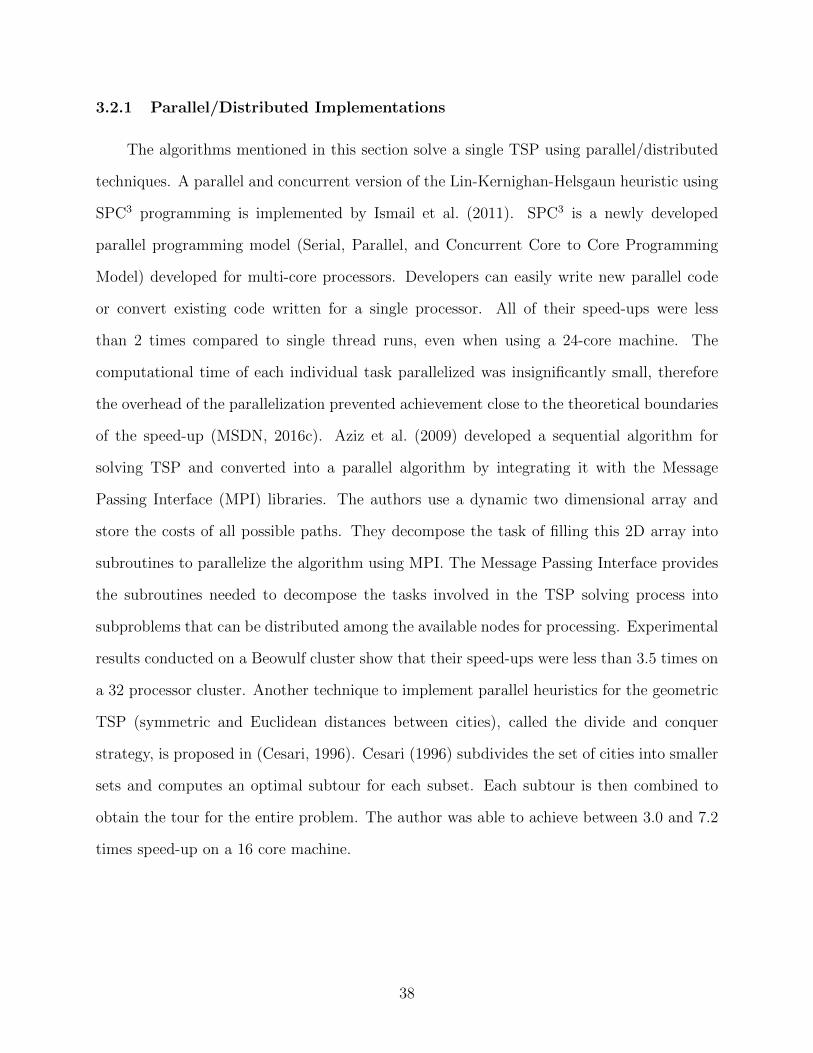
3.2.1 Parallel/Distributed Implementations

The algorithms mentioned in this section solve a single TSP using parallel/distributed

techniques. A parallel and concurrent version of the Lin-Kernighan-Helsgaun heuristic using

SPC3 programming is implemented by Ismail et al. (2011). SPC3 is a newly developed

parallel programming model (Serial, Parallel, and Concurrent Core to Core Programming

Model) developed for multi-core processors. Developers can easily write new parallel code

or convert existing code written for a single processor. All of their speed-ups were less

than 2 times compared to single thread runs, even when using a 24-core machine. The

computational time of each individual task parallelized was insignificantly small, therefore

the overhead of the parallelization prevented achievement close to the theoretical boundaries

of the speed-up (MSDN, 2016c). Aziz et al. (2009) developed a sequential algorithm for

solving TSP and converted into a parallel algorithm by integrating it with the Message

Passing Interface (MPI) libraries. The authors use a dynamic two dimensional array and

store the costs of all possible paths. They decompose the task of filling this 2D array into

subroutines to parallelize the algorithm using MPI. The Message Passing Interface provides

the subroutines needed to decompose the tasks involved in the TSP solving process into

subproblems that can be distributed among the available nodes for processing. Experimental

results conducted on a Beowulf cluster show that their speed-ups were less than 3.5 times on

a 32 processor cluster. Another technique to implement parallel heuristics for the geometric

TSP (symmetric and Euclidean distances between cities), called the divide and conquer

strategy, is proposed in (Cesari, 1996). Cesari (1996) subdivides the set of cities into smaller

sets and computes an optimal subtour for each subset. Each subtour is then combined to

obtain the tour for the entire problem. The author was able to achieve between 3.0 and 7.2

times speed-up on a 16 core machine.

38

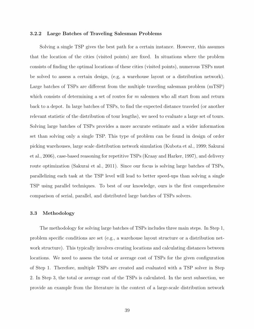
3.2.2 Large Batches of Traveling Salesman Problems

Solving a single TSP gives the best path for a certain instance. However, this assumes

that the location of the cities (visited points) are fixed. In situations where the problem

consists of finding the optimal locations of these cities (visited points), numerous TSPs must

be solved to assess a certain design, (e.g, a warehouse layout or a distribution network).

Large batches of TSPs are different from the multiple traveling salesman problem (mTSP)

which consists of determining a set of routes for m salesmen who all start from and return

back to a depot. In large batches of TSPs, to find the expected distance traveled (or another

relevant statistic of the distribution of tour lengths), we need to evaluate a large set of tours.

Solving large batches of TSPs provides a more accurate estimate and a wider information

set than solving only a single TSP. This type of problem can be found in design of order

picking warehouses, large scale distribution network simulation (Kubota et al., 1999; Sakurai

et al., 2006), case-based reasoning for repetitive TSPs (Kraay and Harker, 1997), and delivery

route optimization (Sakurai et al., 2011). Since our focus is solving large batches of TSPs,

parallelizing each task at the TSP level will lead to better speed-ups than solving a single

TSP using parallel techniques. To best of our knowledge, ours is the first comprehensive

comparison of serial, parallel, and distributed large batches of TSPs solvers.

3.3 Methodology

The methodology for solving large batches of TSPs includes three main steps. In Step 1,

problem specific conditions are set (e.g., a warehouse layout structure or a distribution net-

work structure). This typically involves creating locations and calculating distances between

locations. We need to assess the total or average cost of TSPs for the given configuration

of Step 1. Therefore, multiple TSPs are created and evaluated with a TSP solver in Step

2. In Step 3, the total or average cost of the TSPs is calculated. In the next subsection, we

provide an example from the literature in the context of a large-scale distribution network

39

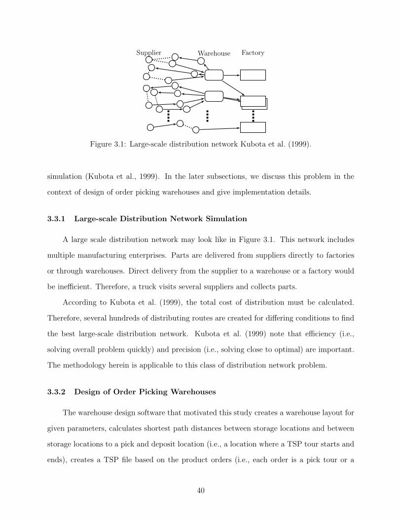
Supplier Warehouse Factory

Figure 3.1: Large-scale distribution network Kubota et al. (1999).

simulation (Kubota et al., 1999). In the later subsections, we discuss this problem in the

context of design of order picking warehouses and give implementation details.

3.3.1 Large-scale Distribution Network Simulation

A large scale distribution network may look like in Figure 3.1. This network includes

multiple manufacturing enterprises. Parts are delivered from suppliers directly to factories

or through warehouses. Direct delivery from the supplier to a warehouse or a factory would

be inefficient. Therefore, a truck visits several suppliers and collects parts.

According to Kubota et al. (1999), the total cost of distribution must be calculated.

Therefore, several hundreds of distributing routes are created for differing conditions to find

the best large-scale distribution network. Kubota et al. (1999) note that efficiency (i.e.,

solving overall problem quickly) and precision (i.e., solving close to optimal) are important.

The methodology herein is applicable to this class of distribution network problem.

3.3.2 Design of Order Picking Warehouses

The warehouse design software that motivated this study creates a warehouse layout for

given parameters, calculates shortest path distances between storage locations and between

storage locations to a pick and deposit location (i.e., a location where a TSP tour starts and

ends), creates a TSP file based on the product orders (i.e., each order is a pick tour or a

40

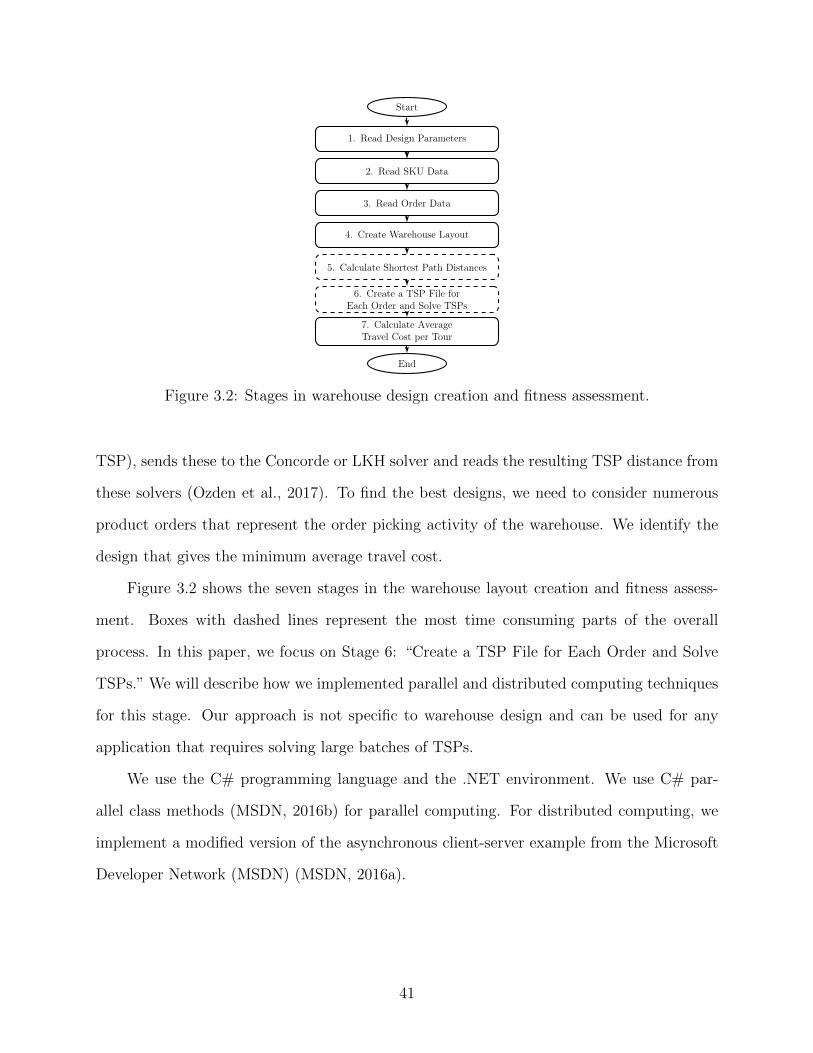
Start

1. Read Design Parameters

2. Read SKU Data

3. Read Order Data

4. Create Warehouse Layout

5. Calculate Shortest Path Distances

6. Create a TSP File forEach Order and Solve TSPs

7. Calculate AverageTravel Cost per Tour

End

Figure 3.2: Stages in warehouse design creation and fitness assessment.

TSP), sends these to the Concorde or LKH solver and reads the resulting TSP distance from

these solvers (Ozden et al., 2017). To find the best designs, we need to consider numerous

product orders that represent the order picking activity of the warehouse. We identify the

design that gives the minimum average travel cost.

Figure 3.2 shows the seven stages in the warehouse layout creation and fitness assess-

ment. Boxes with dashed lines represent the most time consuming parts of the overall

process. In this paper, we focus on Stage 6: “Create a TSP File for Each Order and Solve

TSPs.” We will describe how we implemented parallel and distributed computing techniques

for this stage. Our approach is not specific to warehouse design and can be used for any

application that requires solving large batches of TSPs.

We use the C# programming language and the .NET environment. We use C# par-

allel class methods (MSDN, 2016b) for parallel computing. For distributed computing, we

implement a modified version of the asynchronous client-server example from the Microsoft

Developer Network (MSDN) (MSDN, 2016a).

41

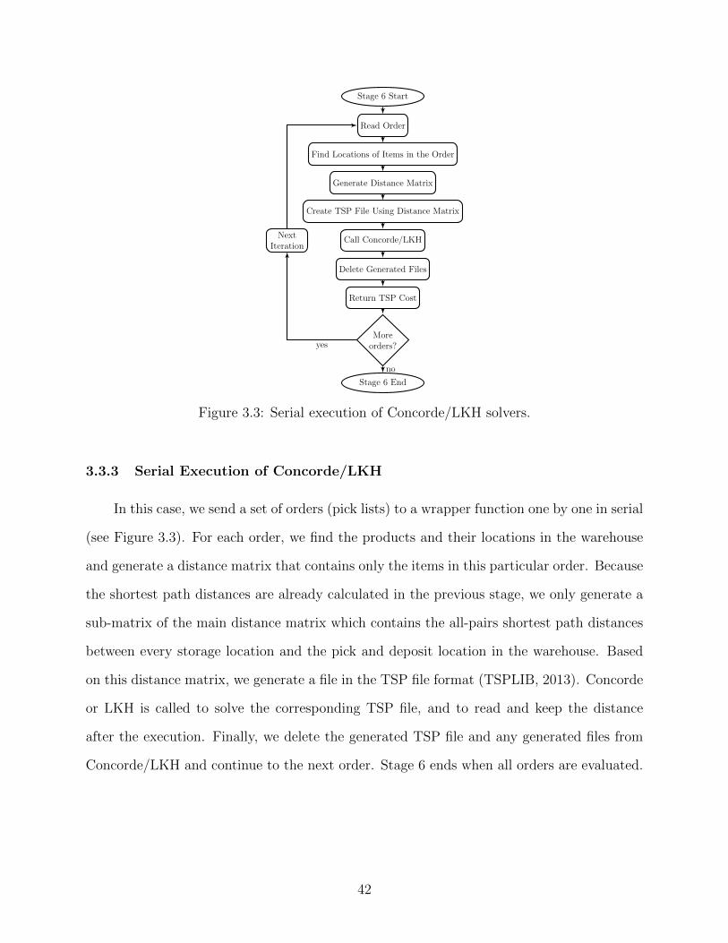
Stage 6 Start

Read Order

Find Locations of Items in the Order

Generate Distance Matrix

Create TSP File Using Distance Matrix

Call Concorde/LKH

Delete Generated Files

Return TSP Cost

Moreorders?

Stage 6 End

NextIteration

yes

no

Figure 3.3: Serial execution of Concorde/LKH solvers.

3.3.3 Serial Execution of Concorde/LKH

In this case, we send a set of orders (pick lists) to a wrapper function one by one in serial

(see Figure 3.3). For each order, we find the products and their locations in the warehouse

and generate a distance matrix that contains only the items in this particular order. Because

the shortest path distances are already calculated in the previous stage, we only generate a

sub-matrix of the main distance matrix which contains the all-pairs shortest path distances

between every storage location and the pick and deposit location in the warehouse. Based

on this distance matrix, we generate a file in the TSP file format (TSPLIB, 2013). Concorde

or LKH is called to solve the corresponding TSP file, and to read and keep the distance

after the execution. Finally, we delete the generated TSP file and any generated files from

Concorde/LKH and continue to the next order. Stage 6 ends when all orders are evaluated.

42

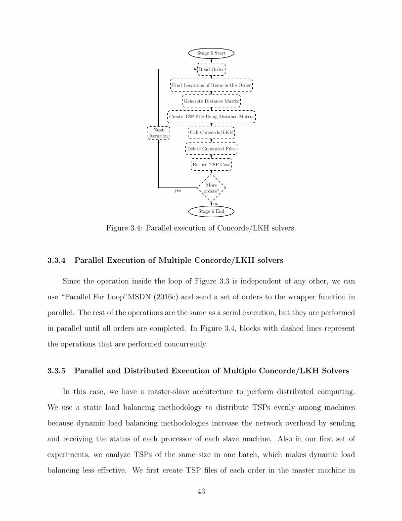
Stage 6 Start

Read Order

Find Locations of Items in the Order

Generate Distance Matrix

Create TSP File Using Distance Matrix

Call Concorde/LKH

Delete Generated Files

Return TSP Cost

Moreorders?

Stage 6 End

NextIteration

yes

no

Figure 3.4: Parallel execution of Concorde/LKH solvers.

3.3.4 Parallel Execution of Multiple Concorde/LKH solvers

Since the operation inside the loop of Figure 3.3 is independent of any other, we can

use “Parallel For Loop”MSDN (2016c) and send a set of orders to the wrapper function in

parallel. The rest of the operations are the same as a serial execution, but they are performed

in parallel until all orders are completed. In Figure 3.4, blocks with dashed lines represent

the operations that are performed concurrently.

3.3.5 Parallel and Distributed Execution of Multiple Concorde/LKH Solvers

In this case, we have a master-slave architecture to perform distributed computing.

We use a static load balancing methodology to distribute TSPs evenly among machines

because dynamic load balancing methodologies increase the network overhead by sending

and receiving the status of each processor of each slave machine. Also in our first set of

experiments, we analyze TSPs of the same size in one batch, which makes dynamic load

balancing less effective. We first create TSP files of each order in the master machine in

43

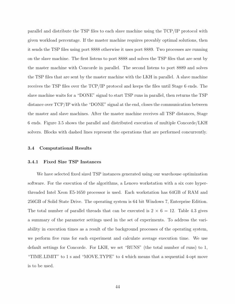
parallel and distribute the TSP files to each slave machine using the TCP/IP protocol with

given workload percentage. If the master machine requires provably optimal solutions, then

it sends the TSP files using port 8888 otherwise it uses port 8889. Two processes are running

on the slave machine. The first listens to port 8888 and solves the TSP files that are sent by

the master machine with Concorde in parallel. The second listens to port 8889 and solves

the TSP files that are sent by the master machine with the LKH in parallel. A slave machine

receives the TSP files over the TCP/IP protocol and keeps the files until Stage 6 ends. The

slave machine waits for a “DONE” signal to start TSP runs in parallel, then returns the TSP

distance over TCP/IP with the “DONE” signal at the end, closes the communication between

the master and slave machines. After the master machine receives all TSP distances, Stage

6 ends. Figure 3.5 shows the parallel and distributed execution of multiple Concorde/LKH

solvers. Blocks with dashed lines represent the operations that are performed concurrently.

3.4 Computational Results

3.4.1 Fixed Size TSP Instances

We have selected fixed sized TSP instances generated using our warehouse optimization

software. For the execution of the algorithms, a Lenovo workstation with a six core hyper-

threaded Intel Xeon E5-1650 processor is used. Each workstation has 64GB of RAM and

256GB of Solid State Drive. The operating system is 64 bit Windows 7, Enterprise Edition.

The total number of parallel threads that can be executed is 2 × 6 = 12. Table 4.3 gives

a summary of the parameter settings used in the set of experiments. To address the vari-

ability in execution times as a result of the background processes of the operating system,

we perform five runs for each experiment and calculate average execution time. We use

default settings for Concorde. For LKH, we set “RUNS” (the total number of runs) to 1,

“TIME LIMIT” to 1 s and “MOVE TYPE” to 4 which means that a sequential 4-opt move

is to be used.

44

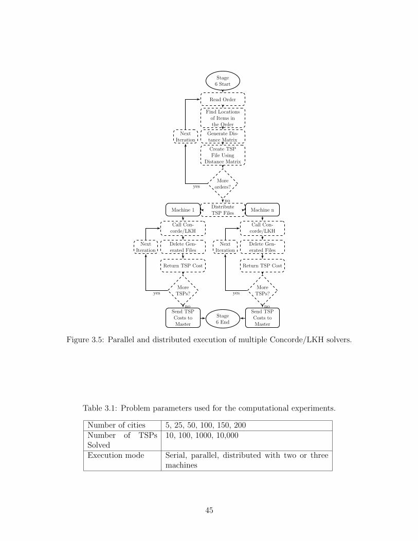
Stage6 Start

Read Order

Find Locationsof Items inthe Order

Generate Dis-tance Matrix

Create TSPFile Using

Distance Matrix

Moreorders?

DistributeTSP Files

Machine 1 Machine n

Call Con-corde/LKH

Call Con-corde/LKH

Delete Gen-erated Files

Delete Gen-erated Files

Return TSP Cost Return TSP Cost

MoreTSPs?

MoreTSPs?

Stage6 End

NextIteration

NextIteration

NextIteration

Send TSPCosts toMaster

Send TSPCosts toMaster

yes

yes yes

no

no no

Figure 3.5: Parallel and distributed execution of multiple Concorde/LKH solvers.

Table 3.1: Problem parameters used for the computational experiments.

Number of cities 5, 25, 50, 100, 150, 200Number of TSPsSolved

10, 100, 1000, 10,000

Execution mode Serial, parallel, distributed with two or threemachines

45

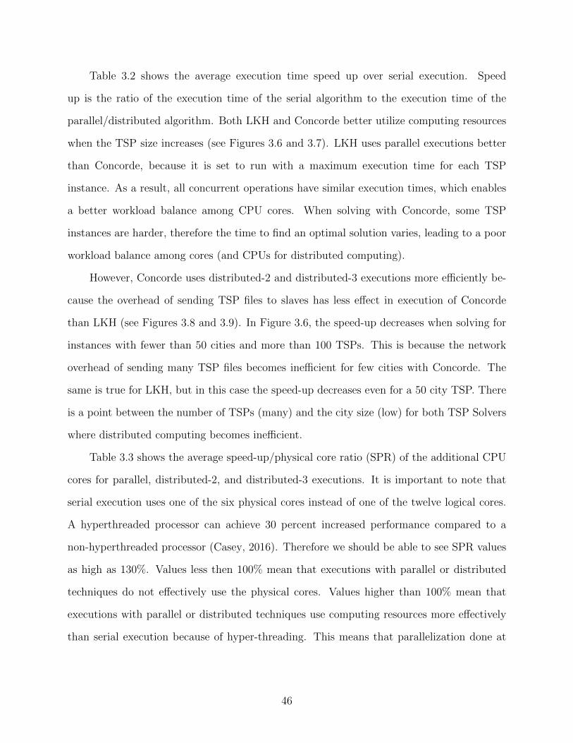
Table 3.2 shows the average execution time speed up over serial execution. Speed

up is the ratio of the execution time of the serial algorithm to the execution time of the

parallel/distributed algorithm. Both LKH and Concorde better utilize computing resources

when the TSP size increases (see Figures 3.6 and 3.7). LKH uses parallel executions better

than Concorde, because it is set to run with a maximum execution time for each TSP

instance. As a result, all concurrent operations have similar execution times, which enables

a better workload balance among CPU cores. When solving with Concorde, some TSP

instances are harder, therefore the time to find an optimal solution varies, leading to a poor

workload balance among cores (and CPUs for distributed computing).

However, Concorde uses distributed-2 and distributed-3 executions more efficiently be-

cause the overhead of sending TSP files to slaves has less effect in execution of Concorde

than LKH (see Figures 3.8 and 3.9). In Figure 3.6, the speed-up decreases when solving for

instances with fewer than 50 cities and more than 100 TSPs. This is because the network

overhead of sending many TSP files becomes inefficient for few cities with Concorde. The

same is true for LKH, but in this case the speed-up decreases even for a 50 city TSP. There

is a point between the number of TSPs (many) and the city size (low) for both TSP Solvers

where distributed computing becomes inefficient.

Table 3.3 shows the average speed-up/physical core ratio (SPR) of the additional CPU

cores for parallel, distributed-2, and distributed-3 executions. It is important to note that

serial execution uses one of the six physical cores instead of one of the twelve logical cores.

A hyperthreaded processor can achieve 30 percent increased performance compared to a

non-hyperthreaded processor (Casey, 2016). Therefore we should be able to see SPR values

as high as 130%. Values less then 100% mean that executions with parallel or distributed

techniques do not effectively use the physical cores. Values higher than 100% mean that

executions with parallel or distributed techniques use computing resources more effectively

than serial execution because of hyper-threading. This means that parallelization done at

46

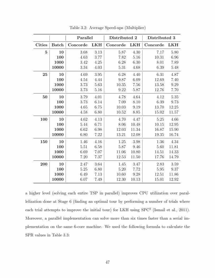
Table 3.2: Average Speed-ups (Multiplier)

Parallel Distributed 2 Distributed 3

Cities Batch Concorde LKH Concorde LKH Concorde LKH

5 10 3.68 3.13 5.87 4.30 7.17 5.80100 4.63 3.77 7.82 5.16 10.31 6.96

1000 3.42 4.25 6.28 6.30 8.01 7.8910000 3.34 4.03 5.31 4.68 6.39 5.48

25 10 4.69 3.95 6.28 4.40 6.31 4.87100 4.54 4.44 9.87 6.09 12.69 7.40

1000 3.73 5.63 10.35 7.56 13.58 9.2910000 3.73 5.16 9.22 5.87 12.76 7.70

50 10 3.79 4.01 4.78 4.64 4.12 5.35100 3.73 6.14 7.09 8.10 6.39 9.73

1000 4.65 6.75 10.03 9.19 13.70 12.2510000 4.58 6.80 10.52 8.85 15.02 11.57

100 10 4.62 4.13 4.70 4.47 5.25 4.66100 5.44 6.71 8.06 10.48 10.15 12.95

1000 6.62 6.98 12.03 11.34 16.87 15.9010000 6.80 7.22 13.21 12.08 19.35 16.74

150 10 1.46 4.16 1.25 3.98 1.36 4.34100 5.51 6.58 5.87 9.46 5.60 11.81

1000 6.69 7.07 11.06 10.80 14.51 14.3310000 7.20 7.37 12.53 11.50 17.76 14.79

200 10 2.47 3.64 1.45 3.47 2.83 3.59100 5.25 6.80 5.20 7.72 5.95 9.37

1000 6.49 7.13 10.60 9.28 12.51 11.8610000 6.07 7.49 12.30 10.13 15.01 12.92

a higher level (solving each entire TSP in parallel) improves CPU utilization over paral-

lelization done at Stage 6 (finding an optimal tour by performing a number of trials where

each trial attempts to improve the initial tour) for LKH using SPC3 (Ismail et al., 2011).

Moreover, a parallel implementation can solve more than six times faster than a serial im-

plementation on the same 6-core machine. We used the following formula to calculate the

SPR values in Table 3.3:

47

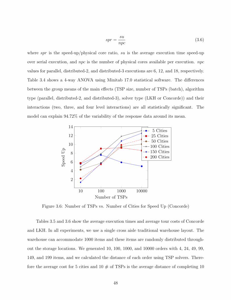
spr =su

npc(3.6)

where spr is the speed-up/physical core ratio, su is the average execution time speed-up

over serial execution, and npc is the number of physical cores available per execution. npc

values for parallel, distributed-2, and distributed-3 executions are 6, 12, and 18, respectively.

Table 3.4 shows a 4-way ANOVA using Minitab 17.0 statistical software. The differences

between the group means of the main effects (TSP size, number of TSPs (batch), algorithm

type (parallel, distributed-2, and distributed-3), solver type (LKH or Concorde)) and their

interactions (two, three, and four level interactions) are all statistically significant. The

model can explain 94.72% of the variability of the response data around its mean.

10 100 1000 10000

2

4

6

8

10

12

14

Number of TSPs

Sp

eed

Up

5 Cities25 Cities50 Cities100 Cities150 Cities200 Cities

Figure 3.6: Number of TSPs vs. Number of Cities for Speed Up (Concorde)

Tables 3.5 and 3.6 show the average execution times and average tour costs of Concorde

and LKH. In all experiments, we use a single cross aisle traditional warehouse layout. The

warehouse can accommodate 1000 items and these items are randomly distributed through-

out the storage locations. We generated 10, 100, 1000, and 10000 orders with 4, 24, 49, 99,

149, and 199 items, and we calculated the distance of each order using TSP solvers. There-

fore the average cost for 5 cities and 10 # of TSPs is the average distance of completing 10

48

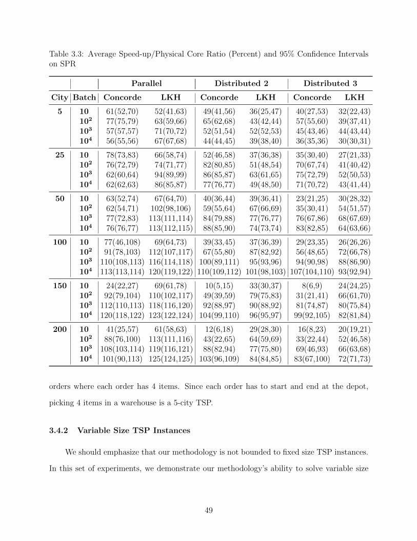
Table 3.3: Average Speed-up/Physical Core Ratio (Percent) and 95% Confidence Intervalson SPR

Parallel Distributed 2 Distributed 3

City Batch Concorde LKH Concorde LKH Concorde LKH

5 10 61(52,70) 52(41,63) 49(41,56) 36(25,47) 40(27,53) 32(22,43)102 77(75,79) 63(59,66) 65(62,68) 43(42,44) 57(55,60) 39(37,41)103 57(57,57) 71(70,72) 52(51,54) 52(52,53) 45(43,46) 44(43,44)104 56(55,56) 67(67,68) 44(44,45) 39(38,40) 36(35,36) 30(30,31)

25 10 78(73,83) 66(58,74) 52(46,58) 37(36,38) 35(30,40) 27(21,33)102 76(72,79) 74(71,77) 82(80,85) 51(48,54) 70(67,74) 41(40,42)103 62(60,64) 94(89,99) 86(85,87) 63(61,65) 75(72,79) 52(50,53)104 62(62,63) 86(85,87) 77(76,77) 49(48,50) 71(70,72) 43(41,44)

50 10 63(52,74) 67(64,70) 40(36,44) 39(36,41) 23(21,25) 30(28,32)102 62(54,71) 102(98,106) 59(55,64) 67(66,69) 35(30,41) 54(51,57)103 77(72,83) 113(111,114) 84(79,88) 77(76,77) 76(67,86) 68(67,69)104 76(76,77) 113(112,115) 88(85,90) 74(73,74) 83(82,85) 64(63,66)

100 10 77(46,108) 69(64,73) 39(33,45) 37(36,39) 29(23,35) 26(26,26)102 91(78,103) 112(107,117) 67(55,80) 87(82,92) 56(48,65) 72(66,78)103 110(108,113) 116(114,118) 100(89,111) 95(93,96) 94(90,98) 88(86,90)104 113(113,114) 120(119,122) 110(109,112) 101(98,103) 107(104,110) 93(92,94)

150 10 24(22,27) 69(61,78) 10(5,15) 33(30,37) 8(6,9) 24(24,25)102 92(79,104) 110(102,117) 49(39,59) 79(75,83) 31(21,41) 66(61,70)103 112(110,113) 118(116,120) 92(88,97) 90(88,92) 81(74,87) 80(75,84)104 120(118,122) 123(122,124) 104(99,110) 96(95,97) 99(92,105) 82(81,84)

200 10 41(25,57) 61(58,63) 12(6,18) 29(28,30) 16(8,23) 20(19,21)102 88(76,100) 113(111,116) 43(22,65) 64(59,69) 33(22,44) 52(46,58)103 108(103,114) 119(116,121) 88(82,94) 77(75,80) 69(46,93) 66(63,68)104 101(90,113) 125(124,125) 103(96,109) 84(84,85) 83(67,100) 72(71,73)

orders where each order has 4 items. Since each order has to start and end at the depot,

picking 4 items in a warehouse is a 5-city TSP.

3.4.2 Variable Size TSP Instances

We should emphasize that our methodology is not bounded to fixed size TSP instances.

In this set of experiments, we demonstrate our methodology’s ability to solve variable size

49

Table 3.4: ANOVA for SPR versus Size, Batch, Algorithm, Solver

Source DF Adj SS Adj MS F-Value P-Value

Size 5 7.6132 1.52264 275.88 0Batch 3 21.4787 7.15956 1297.22 0Algorithm 2 12.0637 6.03184 1092.89 0Solver 1 0.078 0.078 14.13 0Size*Batch 15 7.7685 0.5179 93.84 0Size*Algorithm 10 0.7865 0.07865 14.25 0Size*Solver 5 1.3363 0.26725 48.42 0Batch*Algorithm 6 0.4232 0.07054 12.78 0Batch*Solver 3 0.3713 0.12377 22.42 0Algorithm*Solver 2 1.2914 0.64569 116.99 0Size*Batch*Algorithm 30 0.7685 0.02562 4.64 0Size*Batch*Solver 15 1.524 0.1016 18.41 0Size*Algorithm*Solver 10 0.4784 0.04784 8.67 0Batch*Algorithm*Solver 6 0.5061 0.08435 15.28 0Size*Batch*Algorithm*Solver 30 0.4957 0.01652 2.99 0

Error 576 3.179 0.00552

Total 719 60.1625

S R-sq R-sq(adj) R-sq(pred)

0.0742909 94.72% 93.40% 91.74%

50

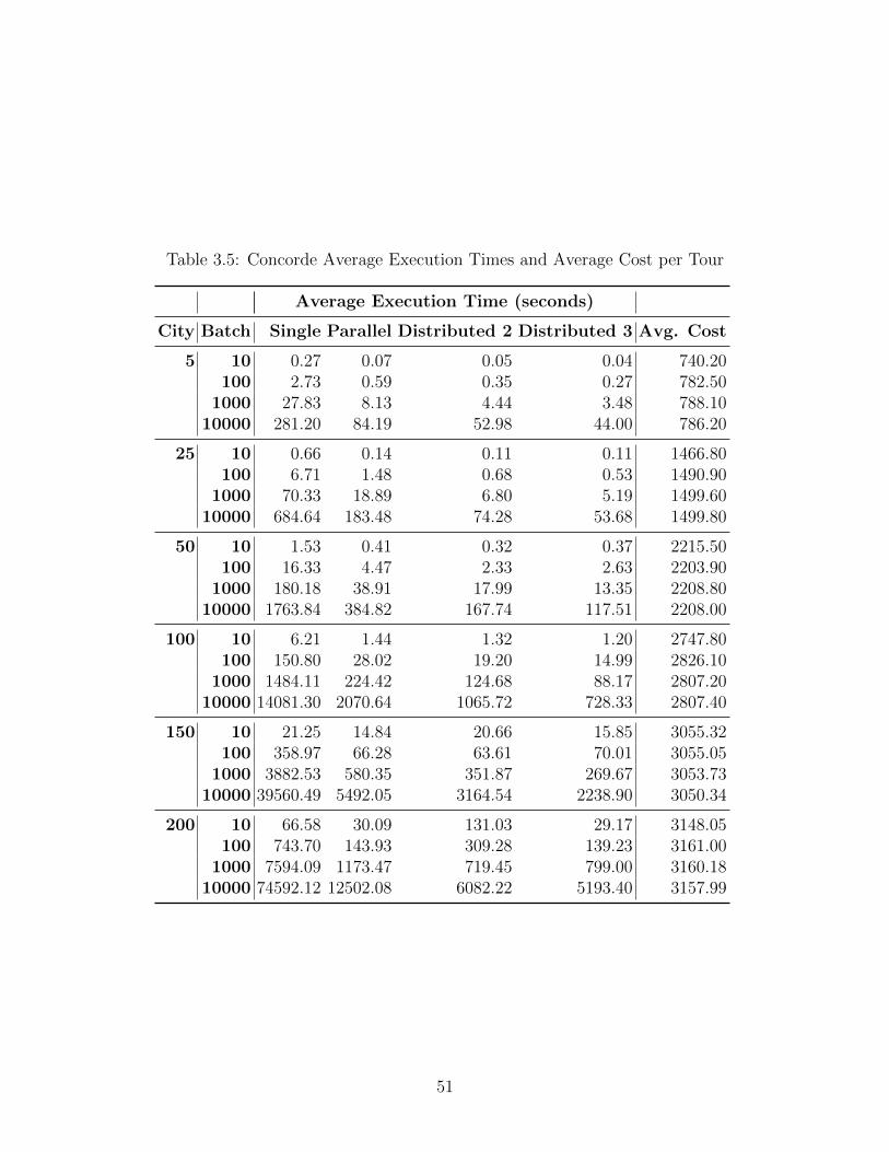
Table 3.5: Concorde Average Execution Times and Average Cost per Tour

Average Execution Time (seconds)

City Batch Single Parallel Distributed 2 Distributed 3 Avg. Cost

5 10 0.27 0.07 0.05 0.04 740.20100 2.73 0.59 0.35 0.27 782.50

1000 27.83 8.13 4.44 3.48 788.1010000 281.20 84.19 52.98 44.00 786.20

25 10 0.66 0.14 0.11 0.11 1466.80100 6.71 1.48 0.68 0.53 1490.90

1000 70.33 18.89 6.80 5.19 1499.6010000 684.64 183.48 74.28 53.68 1499.80

50 10 1.53 0.41 0.32 0.37 2215.50100 16.33 4.47 2.33 2.63 2203.90

1000 180.18 38.91 17.99 13.35 2208.8010000 1763.84 384.82 167.74 117.51 2208.00

100 10 6.21 1.44 1.32 1.20 2747.80100 150.80 28.02 19.20 14.99 2826.10

1000 1484.11 224.42 124.68 88.17 2807.2010000 14081.30 2070.64 1065.72 728.33 2807.40

150 10 21.25 14.84 20.66 15.85 3055.32100 358.97 66.28 63.61 70.01 3055.05

1000 3882.53 580.35 351.87 269.67 3053.7310000 39560.49 5492.05 3164.54 2238.90 3050.34

200 10 66.58 30.09 131.03 29.17 3148.05100 743.70 143.93 309.28 139.23 3161.00

1000 7594.09 1173.47 719.45 799.00 3160.1810000 74592.12 12502.08 6082.22 5193.40 3157.99

51

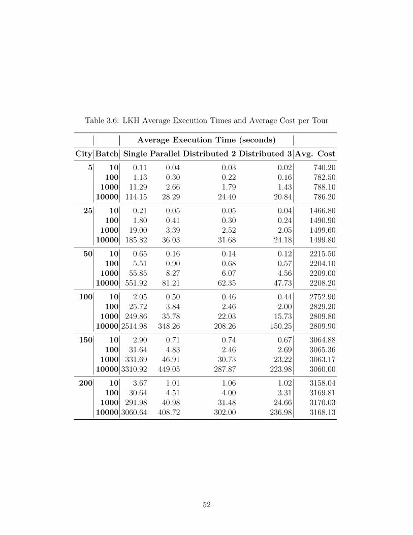
Table 3.6: LKH Average Execution Times and Average Cost per Tour

Average Execution Time (seconds)

City Batch Single Parallel Distributed 2 Distributed 3 Avg. Cost

5 10 0.11 0.04 0.03 0.02 740.20100 1.13 0.30 0.22 0.16 782.50

1000 11.29 2.66 1.79 1.43 788.1010000 114.15 28.29 24.40 20.84 786.20

25 10 0.21 0.05 0.05 0.04 1466.80100 1.80 0.41 0.30 0.24 1490.90

1000 19.00 3.39 2.52 2.05 1499.6010000 185.82 36.03 31.68 24.18 1499.80

50 10 0.65 0.16 0.14 0.12 2215.50100 5.51 0.90 0.68 0.57 2204.10

1000 55.85 8.27 6.07 4.56 2209.0010000 551.92 81.21 62.35 47.73 2208.20

100 10 2.05 0.50 0.46 0.44 2752.90100 25.72 3.84 2.46 2.00 2829.20

1000 249.86 35.78 22.03 15.73 2809.8010000 2514.98 348.26 208.26 150.25 2809.90

150 10 2.90 0.71 0.74 0.67 3064.88100 31.64 4.83 2.46 2.69 3065.36

1000 331.69 46.91 30.73 23.22 3063.1710000 3310.92 449.05 287.87 223.98 3060.00

200 10 3.67 1.01 1.06 1.02 3158.04100 30.64 4.51 4.00 3.31 3169.81

1000 291.98 40.98 31.48 24.66 3170.0310000 3060.64 408.72 302.00 236.98 3168.13

52

10 100 1000 10000

4

6

8

10

12

14

Number of TSPs

Sp

eed

Up

5 Cities25 Cities50 Cities100 Cities150 Cities200 Cities

Figure 3.7: Number of TSPs vs. Number of Cities for Speed Up (LKH)

P D-2 D-340

60

80

100

120

Execution Mode

SP

R(p

erce

nt)

5 Cities25 Cities50 Cities100 Cities150 Cities200 Cities

Figure 3.8: Execution Mode vs. Number of Cities for SPR (Concorde)

TSP instances. These instances are from real order picking data where TSP sizes are dif-

ferent. This real order data set has 10,967 TSPs, the average number of cities visited per

TSP is 10.12, and the largest TSP has 164 cities. The frequency of TSP sizes is shown

in Figure 3.10. Because of variable TSP sizes, equal distribution of TSPs among identical

machines may create overloaded machines and increase the total makespan. Therefore, we

compare an equal distribution rule (EDR) against a well known task assignment rule, the

longest processing time (LPT) rule (Graham, 1969). In LPT, jobs (TSPs) are sorted by

53

P D-2 D-3

40

60

80

100

120

Execution Mode

SP

R(p

erce

nt)

5 Cities25 Cities50 Cities100 Cities150 Cities200 Cities

Figure 3.9: Execution Mode vs. Number of Cities for SPR (LKH)

problem size (as a proxy for processing time, which we do not know yet) and assigned to the

machine with the earliest end time so far. In worst case scenario, the algorithm achieves a

makespan of 4/3 − 1/3(m)OPT where m is the number of machines (i.e., LPT produces a

makespan that is at most 33% worse than optimal assignment). We perform five replications

for each experiment. Two important things affect the results of these runs: the order of the

TSPs in EDR and the estimation of processing time by size of TSP. In some cases, a 40-city

TSP can be much harder than a 41-city TSP. Also, a two machine EDR may perform close

to optimal, whereas a three machine EDR can be quite suboptimal. The 3-way ANOVA in

Table 3.8 shows that all main factors and the Machines*Solver interaction are significant.

Other two-way interactions and the three way interaction are insignificant. The model ex-

plains 99.65% of the variability of the response data around its mean. Figure 3.11 shows

the statistically significant effects — all three main effects and the two way interaction for

Machines*Solver. The difference between the means of the TSP solvers is more pronounced

than the other two main effects; LKH is nearly three times faster than Concorde. Obviously,

increasing from two to three machines reduces the time needed. The 1.8 second difference

between the means of EDR and LPT is statistically significant, showing the benefit of using

54

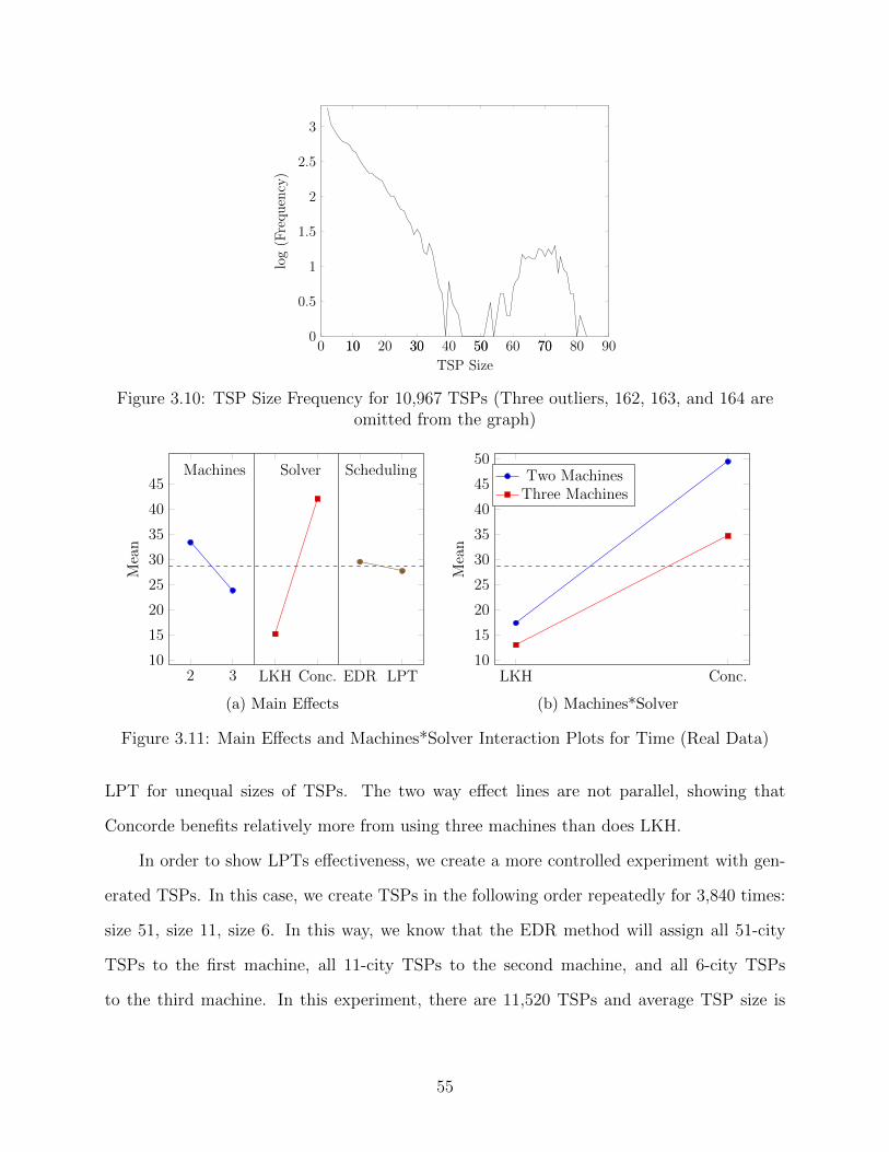
0 10 20 30 40 50 60 70 80 900

0.5

1

1.5

2

2.5

3

10 30 50 70

TSP Size

log

(Fre

qu

ency

)

Figure 3.10: TSP Size Frequency for 10,967 TSPs (Three outliers, 162, 163, and 164 areomitted from the graph)

2 3 LKH Conc. EDR LPT10

15

20

25

30

35

40

45Machines Solver Scheduling

Mea

n

(a) Main Effects

LKH Conc.10

15

20

25

30

35

40

45

50M

ean

Two MachinesThree Machines

(b) Machines*Solver

Figure 3.11: Main Effects and Machines*Solver Interaction Plots for Time (Real Data)

LPT for unequal sizes of TSPs. The two way effect lines are not parallel, showing that

Concorde benefits relatively more from using three machines than does LKH.

In order to show LPTs effectiveness, we create a more controlled experiment with gen-

erated TSPs. In this case, we create TSPs in the following order repeatedly for 3,840 times:

size 51, size 11, size 6. In this way, we know that the EDR method will assign all 51-city

TSPs to the first machine, all 11-city TSPs to the second machine, and all 6-city TSPs

to the third machine. In this experiment, there are 11,520 TSPs and average TSP size is

55

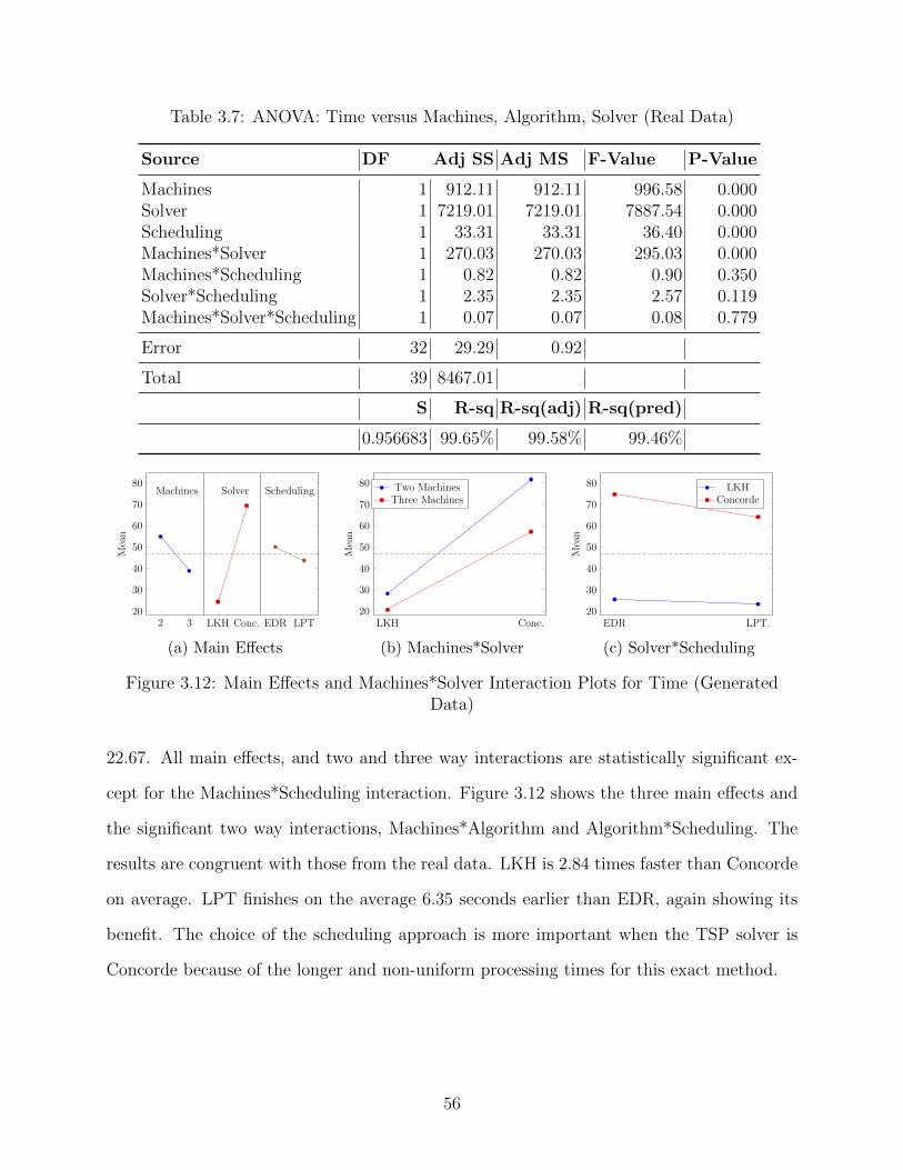
Table 3.7: ANOVA: Time versus Machines, Algorithm, Solver (Real Data)

Source DF Adj SS Adj MS F-Value P-Value

Machines 1 912.11 912.11 996.58 0.000Solver 1 7219.01 7219.01 7887.54 0.000Scheduling 1 33.31 33.31 36.40 0.000Machines*Solver 1 270.03 270.03 295.03 0.000Machines*Scheduling 1 0.82 0.82 0.90 0.350Solver*Scheduling 1 2.35 2.35 2.57 0.119Machines*Solver*Scheduling 1 0.07 0.07 0.08 0.779

Error 32 29.29 0.92

Total 39 8467.01

S R-sq R-sq(adj) R-sq(pred)

0.956683 99.65% 99.58% 99.46%

2 3 LKH Conc. EDR LPT20

30

40

50

60

70

80Machines Solver Scheduling

Mea

n

(a) Main Effects

LKH Conc.20

30

40

50

60

70

80

Mea

n

Two MachinesThree Machines

(b) Machines*Solver

EDR LPT.20

30

40

50

60

70

80

Mea

n

LKHConcorde

(c) Solver*Scheduling

Figure 3.12: Main Effects and Machines*Solver Interaction Plots for Time (GeneratedData)

22.67. All main effects, and two and three way interactions are statistically significant ex-

cept for the Machines*Scheduling interaction. Figure 3.12 shows the three main effects and

the significant two way interactions, Machines*Algorithm and Algorithm*Scheduling. The

results are congruent with those from the real data. LKH is 2.84 times faster than Concorde

on average. LPT finishes on the average 6.35 seconds earlier than EDR, again showing its

benefit. The choice of the scheduling approach is more important when the TSP solver is

Concorde because of the longer and non-uniform processing times for this exact method.

56

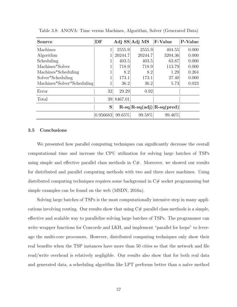
Table 3.8: ANOVA: Time versus Machines, Algorithm, Solver (Generated Data)

Source DF Adj SS Adj MS F-Value P-Value

Machines 1 2555.9 2555.9 404.55 0.000Algorithm 1 20244.7 20244.7 3204.36 0.000Scheduling 1 403.5 403.5 63.87 0.000Machines*Solver 1 718.9 718.9 113.79 0.000Machines*Scheduling 1 8.2 8.2 1.29 0.264Solver*Scheduling 1 173.1 173.1 27.40 0.000Machines*Solver*Scheduling 1 36.2 36.2 5.73 0.023

Error 32 29.29 0.92

Total 39 8467.01

S R-sq R-sq(adj) R-sq(pred)

0.956683 99.65% 99.58% 99.46%

3.5 Conclusions

We presented how parallel computing techniques can significantly decrease the overall

computational time and increase the CPU utilization for solving large batches of TSPs

using simple and effective parallel class methods in C#. Moreover, we showed our results

for distributed and parallel computing methods with two and three slave machines. Using

distributed computing techniques requires some background in C# socket programming but

simple examples can be found on the web (MSDN, 2016a).

Solving large batches of TSPs is the most computationally intensive step in many appli-

cations involving routing. Our results show that using C# parallel class methods is a simple,

effective and scalable way to parallelize solving large batches of TSPs. The programmer can

write wrapper functions for Concorde and LKH, and implement “parallel for loops” to lever-

age the multi-core processors. However, distributed computing techniques only show their

real benefits when the TSP instances have more than 50 cities so that the network and file

read/write overhead is relatively negligible. Our results also show that for both real data

and generated data, a scheduling algorithm like LPT performs better than a naıve method

57

like EDR even though the method used for estimating processing times of TSPs is not very

accurate (TSP size, in this case).

The Lin-Kernighan Heuristic (LKH) can be selected over the Concorde TSP Solver

when optimality is desired but not required. In our results, LKH is 24.37, 30.59, 20.14,

and 21.91 times faster than Concorde on average in single, parallel, 2-computer distributed,

and 3-computer distributed runs for solving 10,000 200-city TSPs, respectively. The average

optimality gap is less than 0.34% per run.

58

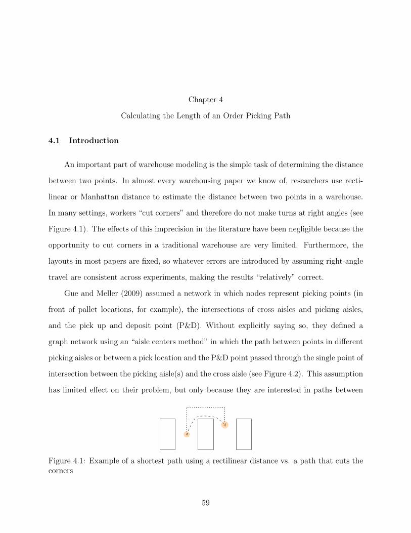
Chapter 4

Calculating the Length of an Order Picking Path

4.1 Introduction

An important part of warehouse modeling is the simple task of determining the distance

between two points. In almost every warehousing paper we know of, researchers use recti-

linear or Manhattan distance to estimate the distance between two points in a warehouse.

In many settings, workers “cut corners” and therefore do not make turns at right angles (see

Figure 4.1). The effects of this imprecision in the literature have been negligible because the

opportunity to cut corners in a traditional warehouse are very limited. Furthermore, the

layouts in most papers are fixed, so whatever errors are introduced by assuming right-angle

travel are consistent across experiments, making the results “relatively” correct.

Gue and Meller (2009) assumed a network in which nodes represent picking points (in

front of pallet locations, for example), the intersections of cross aisles and picking aisles,

and the pick up and deposit point (P&D). Without explicitly saying so, they defined a

graph network using an “aisle centers method” in which the path between points in different

picking aisles or between a pick location and the P&D point passed through the single point of

intersection between the picking aisle(s) and the cross aisle (see Figure 4.2). This assumption

has limited effect on their problem, but only because they are interested in paths between

s

d

Figure 4.1: Example of a shortest path using a rectilinear distance vs. a path that cuts thecorners

59

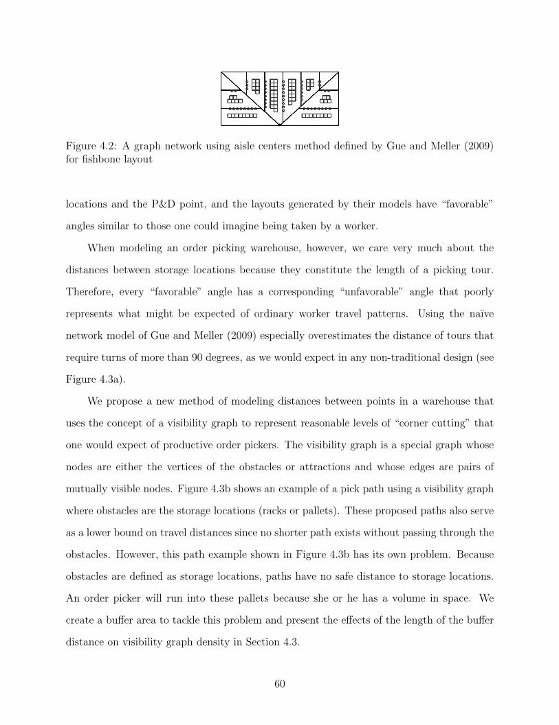
Figure 4.2: A graph network using aisle centers method defined by Gue and Meller (2009)for fishbone layout

locations and the P&D point, and the layouts generated by their models have “favorable”

angles similar to those one could imagine being taken by a worker.

When modeling an order picking warehouse, however, we care very much about the

distances between storage locations because they constitute the length of a picking tour.

Therefore, every “favorable” angle has a corresponding “unfavorable” angle that poorly

represents what might be expected of ordinary worker travel patterns. Using the naıve

network model of Gue and Meller (2009) especially overestimates the distance of tours that

require turns of more than 90 degrees, as we would expect in any non-traditional design (see

Figure 4.3a).

We propose a new method of modeling distances between points in a warehouse that

uses the concept of a visibility graph to represent reasonable levels of “corner cutting” that

one would expect of productive order pickers. The visibility graph is a special graph whose

nodes are either the vertices of the obstacles or attractions and whose edges are pairs of

mutually visible nodes. Figure 4.3b shows an example of a pick path using a visibility graph

where obstacles are the storage locations (racks or pallets). These proposed paths also serve

as a lower bound on travel distances since no shorter path exists without passing through the

obstacles. However, this path example shown in Figure 4.3b has its own problem. Because

obstacles are defined as storage locations, paths have no safe distance to storage locations.

An order picker will run into these pallets because she or he has a volume in space. We

create a buffer area to tackle this problem and present the effects of the length of the buffer

distance on visibility graph density in Section 4.3.

60

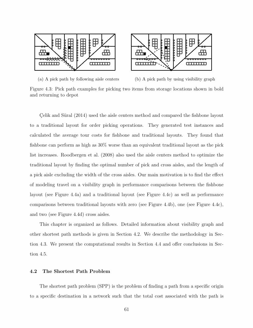
(a) A pick path by following aisle centers (b) A pick path by using visibility graph

Figure 4.3: Pick path examples for picking two items from storage locations shown in boldand returning to depot

Celik and Sural (2014) used the aisle centers method and compared the fishbone layout

to a traditional layout for order picking operations. They generated test instances and

calculated the average tour costs for fishbone and traditional layouts. They found that

fishbone can perform as high as 30% worse than an equivalent traditional layout as the pick

list increases. Roodbergen et al. (2008) also used the aisle centers method to optimize the

traditional layout by finding the optimal number of pick and cross aisles, and the length of

a pick aisle excluding the width of the cross aisles. Our main motivation is to find the effect

of modeling travel on a visibility graph in performance comparisons between the fishbone

layout (see Figure 4.4a) and a traditional layout (see Figure 4.4c) as well as performance

comparisons between traditional layouts with zero (see Figure 4.4b), one (see Figure 4.4c),

and two (see Figure 4.4d) cross aisles.

This chapter is organized as follows. Detailed information about visibility graph and

other shortest path methods is given in Section 4.2. We describe the methodology in Sec-

tion 4.3. We present the computational results in Section 4.4 and offer conclusions in Sec-

tion 4.5.

4.2 The Shortest Path Problem

The shortest path problem (SPP) is the problem of finding a path from a specific origin

to a specific destination in a network such that the total cost associated with the path is

61

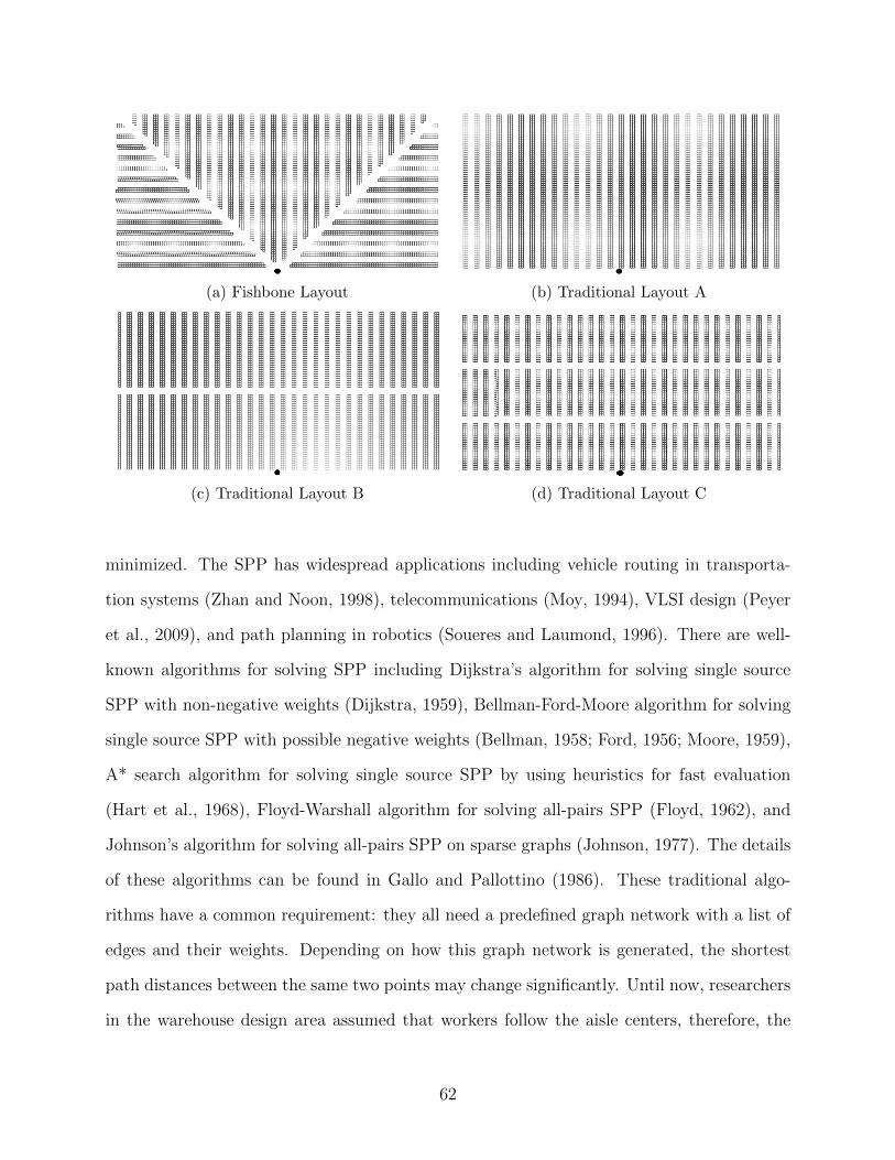
(a) Fishbone Layout (b) Traditional Layout A

(c) Traditional Layout B (d) Traditional Layout C

minimized. The SPP has widespread applications including vehicle routing in transporta-

tion systems (Zhan and Noon, 1998), telecommunications (Moy, 1994), VLSI design (Peyer

et al., 2009), and path planning in robotics (Soueres and Laumond, 1996). There are well-

known algorithms for solving SPP including Dijkstra’s algorithm for solving single source

SPP with non-negative weights (Dijkstra, 1959), Bellman-Ford-Moore algorithm for solving

single source SPP with possible negative weights (Bellman, 1958; Ford, 1956; Moore, 1959),

A* search algorithm for solving single source SPP by using heuristics for fast evaluation

(Hart et al., 1968), Floyd-Warshall algorithm for solving all-pairs SPP (Floyd, 1962), and

Johnson’s algorithm for solving all-pairs SPP on sparse graphs (Johnson, 1977). The details

of these algorithms can be found in Gallo and Pallottino (1986). These traditional algo-

rithms have a common requirement: they all need a predefined graph network with a list of

edges and their weights. Depending on how this graph network is generated, the shortest

path distances between the same two points may change significantly. Until now, researchers

in the warehouse design area assumed that workers follow the aisle centers, therefore, the

62

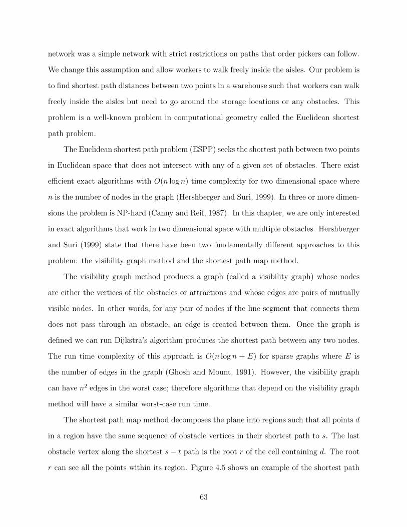
network was a simple network with strict restrictions on paths that order pickers can follow.

We change this assumption and allow workers to walk freely inside the aisles. Our problem is

to find shortest path distances between two points in a warehouse such that workers can walk

freely inside the aisles but need to go around the storage locations or any obstacles. This

problem is a well-known problem in computational geometry called the Euclidean shortest

path problem.

The Euclidean shortest path problem (ESPP) seeks the shortest path between two points

in Euclidean space that does not intersect with any of a given set of obstacles. There exist

efficient exact algorithms with O(n log n) time complexity for two dimensional space where

n is the number of nodes in the graph (Hershberger and Suri, 1999). In three or more dimen-

sions the problem is NP-hard (Canny and Reif, 1987). In this chapter, we are only interested

in exact algorithms that work in two dimensional space with multiple obstacles. Hershberger

and Suri (1999) state that there have been two fundamentally different approaches to this

problem: the visibility graph method and the shortest path map method.

The visibility graph method produces a graph (called a visibility graph) whose nodes

are either the vertices of the obstacles or attractions and whose edges are pairs of mutually

visible nodes. In other words, for any pair of nodes if the line segment that connects them

does not pass through an obstacle, an edge is created between them. Once the graph is

defined we can run Dijkstra’s algorithm produces the shortest path between any two nodes.

The run time complexity of this approach is O(n log n + E) for sparse graphs where E is

the number of edges in the graph (Ghosh and Mount, 1991). However, the visibility graph

can have n2 edges in the worst case; therefore algorithms that depend on the visibility graph

method will have a similar worst-case run time.

The shortest path map method decomposes the plane into regions such that all points d

in a region have the same sequence of obstacle vertices in their shortest path to s. The last

obstacle vertex along the shortest s− t path is the root r of the cell containing d. The root

r can see all the points within its region. Figure 4.5 shows an example of the shortest path

63

s

d

rv

Figure 4.5: A shortest path map with respect to source point s within a polygonal domainwith 3 obstacles. The heavy dashed path indicates the shortest s− d path, which reaches dvia the root r of its cell. Extension segments are shown thin and dotted.

map. Point s reaches d via obstacle vertices v and r. In this example, vertex r is the root of

the region containing d. Hershberger’s algorithm computes shortest paths in the presence of

polygonal obstacles in O(n log n) time and space where n is the number of nodes in graph.

For a detailed review of algorithms that use the visibility graph method or the shortest path

map method, see Toth et al. (2004).

Although Hershberger’s algorithm has a better worst-case running time, we implemented

the visibility graph method because it is easier to understand and implement than the short-

est path map method. Our main aim is to show how paths using the visibility graph method

can affect the performance comparisons between traditional and fishbone layouts as well as

performance comparisons between traditional layouts with zero, one, and two cross aisles.

Computational efficiency is not the main target of this chapter.

4.3 Methodology

In our first set of experiments, we would like to see if the visibility graph method affects

the comparisons between fishbone and traditional layout. We use the average tour cost for a

set of test instances as the performance metric. We developed a warehouse modeling system

to calculate the average tour cost of test instances for a given warehouse environment. This

system can compare any warehouse layout with the visibility graph method or the aisle

64

centers method. The following nine steps are performed in this system to calculate the

average tour cost.

In Step 1, we create exterior aisles for a given width and depth of the warehouse. These

exterior aisles serve as the boundaries of the rectangle-shaped warehouse.

In Step 2, we create cross aisles using exterior and interior points. An exterior point

lies on the boundaries of the warehouse (i.e., exterior aisles) and an interior point lies inside

the boundaries of the warehouse. Cross aisles divide the warehouse into regions.

In Step 3, we create pick aisles, pick locations, and storage locations for each region.

We assume that items on both sides of a pick aisle may be accessed with negligible lateral

movement. Figure 4.6 illustrates a warehouse.

Cross AislePolygon/Buffer Area (2ft.) Pick Aisle

P&D Point

Pick Location

Storage Location

Exterior Aisle

Figure 4.6: Representation of a warehouse. This particular fishbone layout has a single P&Dpoint, 67 storage locations, 51 pick locations, 9 pick aisles, 2 cross aisles, and 4 exterior aisles.The lines that represent the aisle centers are both used for building the warehouse structure(i.e., storage locations and pick locations) and finding the shortest path distances with theaisle centers method.

In Step 4, we calculate polygons that will be used in the visibility graph calculation. In

this step, we create the polygons considering a buffer distance. Corners of the polygons are

also included as a node in the visibility graph. When buffer distance increases the polygons

65

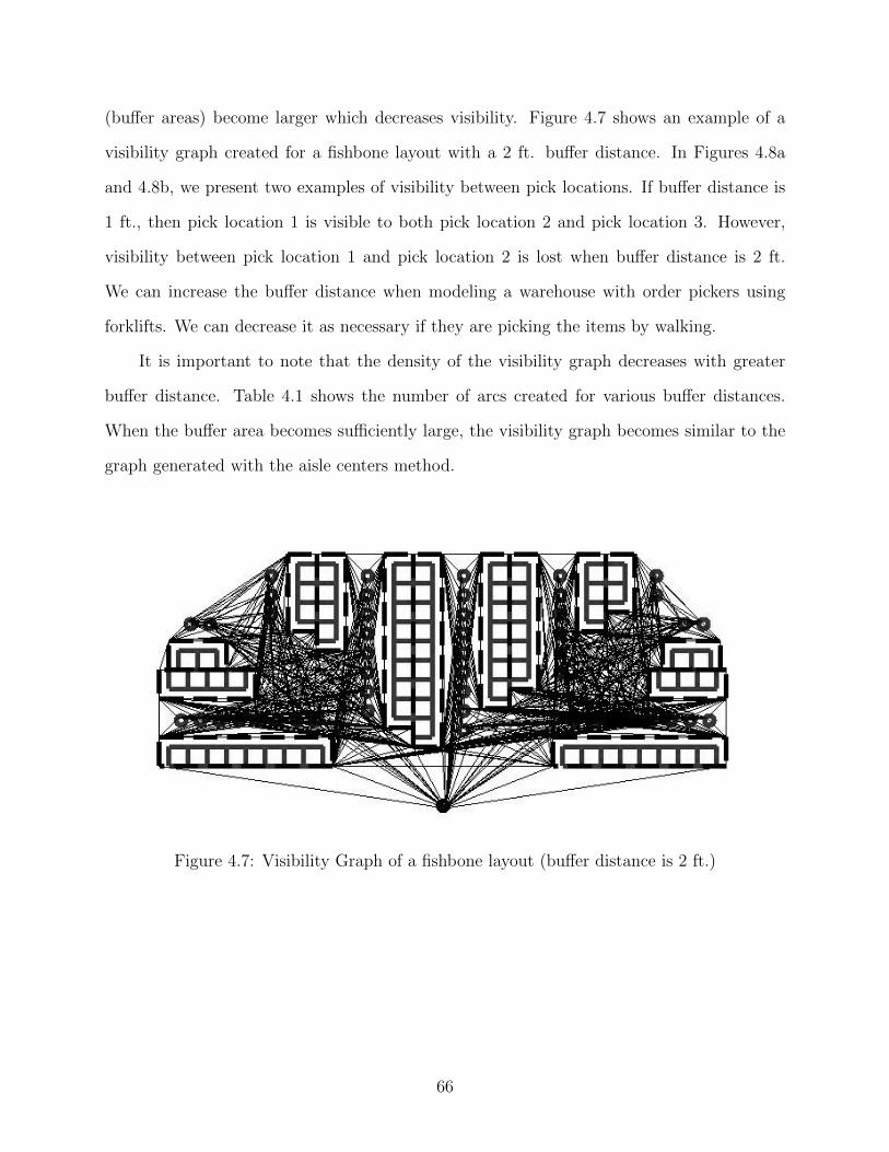
(buffer areas) become larger which decreases visibility. Figure 4.7 shows an example of a

visibility graph created for a fishbone layout with a 2 ft. buffer distance. In Figures 4.8a

and 4.8b, we present two examples of visibility between pick locations. If buffer distance is

1 ft., then pick location 1 is visible to both pick location 2 and pick location 3. However,

visibility between pick location 1 and pick location 2 is lost when buffer distance is 2 ft.

We can increase the buffer distance when modeling a warehouse with order pickers using

forklifts. We can decrease it as necessary if they are picking the items by walking.

It is important to note that the density of the visibility graph decreases with greater

buffer distance. Table 4.1 shows the number of arcs created for various buffer distances.

When the buffer area becomes sufficiently large, the visibility graph becomes similar to the

graph generated with the aisle centers method.

Figure 4.7: Visibility Graph of a fishbone layout (buffer distance is 2 ft.)

66

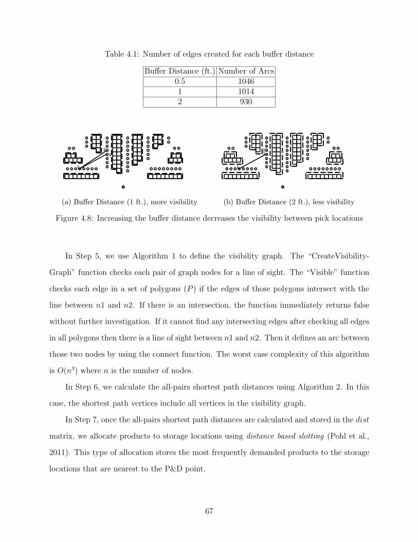
Table 4.1: Number of edges created for each buffer distance

Buffer Distance (ft.) Number of Arcs0.5 10461 10142 930

1

23

(a) Buffer Distance (1 ft.), more visibility

1

23

(b) Buffer Distance (2 ft.), less visibility

Figure 4.8: Increasing the buffer distance decreases the visibility between pick locations

In Step 5, we use Algorithm 1 to define the visibility graph. The “CreateVisibility-

Graph” function checks each pair of graph nodes for a line of sight. The “Visible” function

checks each edge in a set of polygons (P ) if the edges of those polygons intersect with the

line between n1 and n2. If there is an intersection, the function immediately returns false

without further investigation. If it cannot find any intersecting edges after checking all edges

in all polygons then there is a line of sight between n1 and n2. Then it defines an arc between

those two nodes by using the connect function. The worst case complexity of this algorithm

is O(n3) where n is the number of nodes.

In Step 6, we calculate the all-pairs shortest path distances using Algorithm 2. In this

case, the shortest path vertices include all vertices in the visibility graph.

In Step 7, once the all-pairs shortest path distances are calculated and stored in the dist

matrix, we allocate products to storage locations using distance based slotting (Pohl et al.,

2011). This type of allocation stores the most frequently demanded products to the storage

locations that are nearest to the P&D point.

67

Algorithm 1 Visibility Graph Calculation

function CreateVisibilityGraph(void)for (i := 0;i < Count(G);i← i+ 1) do

for (j := 0;j < i;j ← j + 1) doif V isible(G[i], G[j]) then

Connect(G[i], G[j])end if

end forend for

end function

function Visible(n1, n2)for (i := 0;i < Count(P );i← i+ 1) do

for all (edge in P [i]) doif Intersect(n1, n2, edge) then

return falseend if

end forend forreturn true

end function

function Connect(n1, n2)n1.AddtoConnectionList(n2)n2.AddtoConnectionList(n1)

end function

68

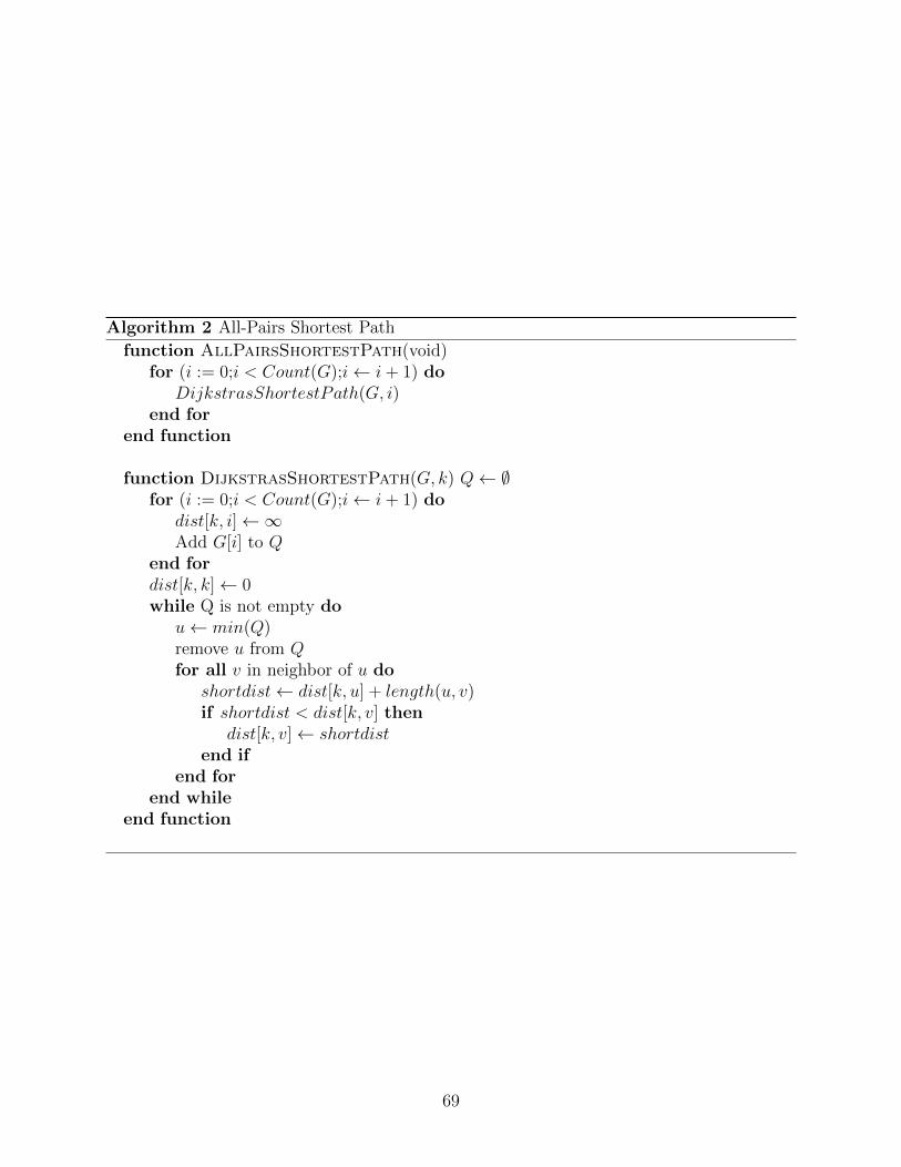
Algorithm 2 All-Pairs Shortest Path

function AllPairsShortestPath(void)for (i := 0;i < Count(G);i← i+ 1) do

DijkstrasShortestPath(G, i)end for

end function

function DijkstrasShortestPath(G, k) Q← ∅for (i := 0;i < Count(G);i← i+ 1) do

dist[k, i]←∞Add G[i] to Q

end fordist[k, k]← 0while Q is not empty do

u← min(Q)remove u from Qfor all v in neighbor of u do

shortdist← dist[k, u] + length(u, v)if shortdist < dist[k, v] then

dist[k, v]← shortdistend if

end forend while

end function

69

In Step 8, we generate a distance matrix for each order in the list of orders by using

a subset of the dist matrix. This distance matrix contains the shortest path distances

between every storage location that needs to be visited in the warehouse and the P&D

point. Finding the shortest tour distance in a warehouse for an order is an example of a

Traveling Salesman Problem (TSP). We obtain optimal travel distances using the Concorde

TSP solver (Applegate et al., 2007).

In Step 9, the average of all TSP costs is used as a fitness function for a given warehouse

layout. This is the final step for calculating the performance metric of a given test instance

for a given warehouse layout.

4.4 Results

In this section, we describe our computational experiments aimed at achieving three

objectives. First, we would like to see how the results of fishbone and traditional layout

comparison would change for various pick lists with a turnover based storage policy and

random storage policy if the visibility graph methods is used, rather than the aisle centers

method. Second, we would like to see how the size of the warehouse affects the comparison

of the visibility graph method and the aisle centers method under a random storage policy.

Lastly, we would like to compare zero, one, and two cross aisle traditional layouts with

both methods (the visibility graph method and the aisle centers method) and see if the best

layout that achieves the minimum average tour cost changes for various warehouse sizes and

demand skewness.

To evaluate the effect of the visibility graph method in average travel cost, the percent

improvement of a fishbone layout (PIFishbone) over a traditional one cross aisle layout (see

Figure 4.4c) is calculated as follows:

PIFishbone =ZTraditional − ZFishbone

ZTraditional

(4.1)

70

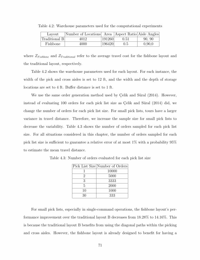
Table 4.2: Warehouse parameters used for the computational experiments

Layout Number of Locations Area Aspect Ratio Aisle AnglesTraditional B 4012 191260 0.51 90, 90

Fishbone 4000 196420 0.5 0,90,0

where ZFishbone and ZTraditional refer to the average travel cost for the fishbone layout and

the traditional layout, respectively.

Table 4.2 shows the warehouse parameters used for each layout. For each instance, the

width of the pick and cross aisles is set to 12 ft, and the width and the depth of storage

locations are set to 4 ft. Buffer distance is set to 1 ft.

We use the same order generation method used by Celik and Sural (2014). However,

instead of evaluating 100 orders for each pick list size as Celik and Sural (2014) did, we

change the number of orders for each pick list size. For small pick lists, tours have a larger

variance in travel distance. Therefore, we increase the sample size for small pick lists to

decrease the variability. Table 4.3 shows the number of orders sampled for each pick list

size. For all situations considered in this chapter, the number of orders sampled for each

pick list size is sufficient to guarantee a relative error of at most 1% with a probability 95%

to estimate the mean travel distance.

Table 4.3: Number of orders evaluated for each pick list size

Pick List Size Number of Orders1 100002 50003 33335 200010 100030 333

For small pick lists, especially in single-command operations, the fishbone layout’s per-

formance improvement over the traditional layout B decreases from 18.28% to 14.16%. This

is because the traditional layout B benefits from using the diagonal paths within the picking

and cross aisles. However, the fishbone layout is already designed to benefit for having a

71

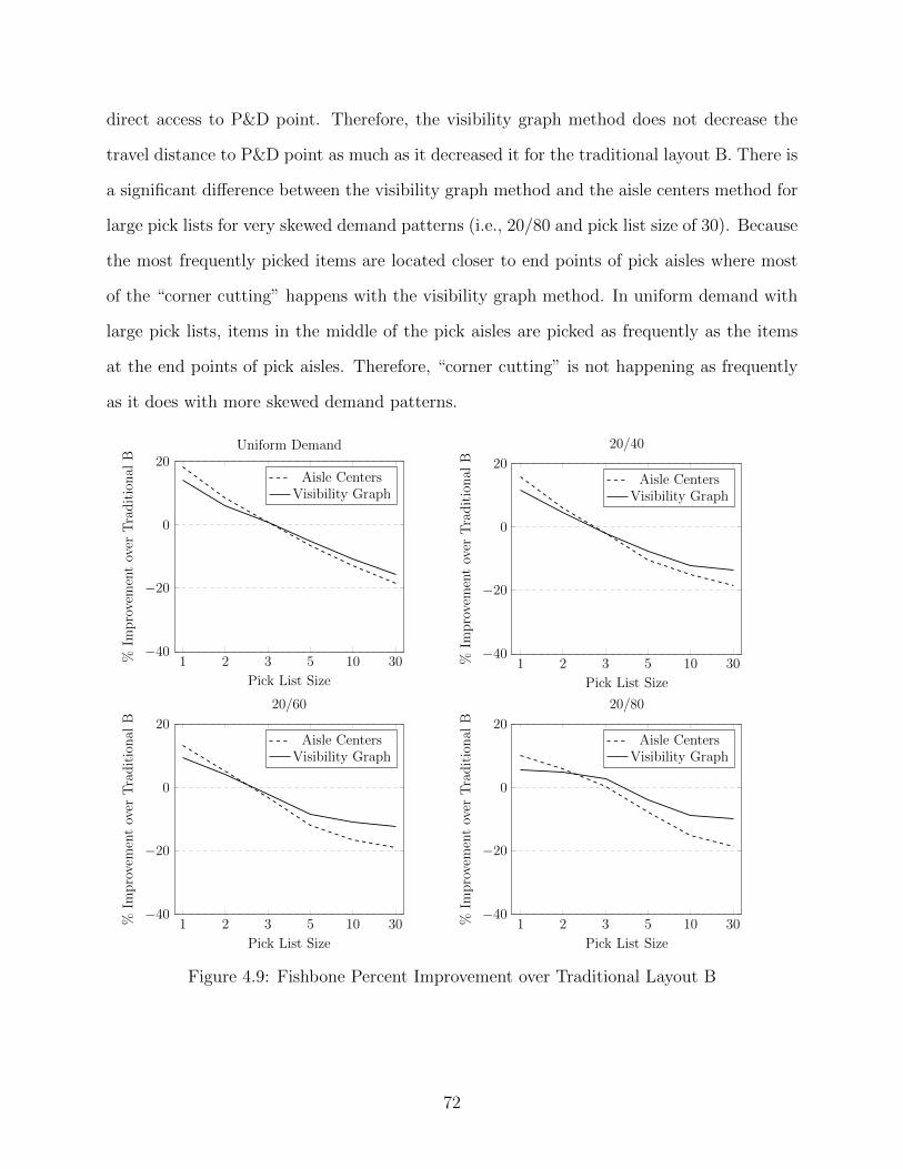
direct access to P&D point. Therefore, the visibility graph method does not decrease the

travel distance to P&D point as much as it decreased it for the traditional layout B. There is

a significant difference between the visibility graph method and the aisle centers method for

large pick lists for very skewed demand patterns (i.e., 20/80 and pick list size of 30). Because

the most frequently picked items are located closer to end points of pick aisles where most

of the “corner cutting” happens with the visibility graph method. In uniform demand with

large pick lists, items in the middle of the pick aisles are picked as frequently as the items

at the end points of pick aisles. Therefore, “corner cutting” is not happening as frequently

as it does with more skewed demand patterns.

1 2 3 5 10 30−40

−20

0

20

Pick List Size

%Im

pro

vem

ent

over

Tra

dit

ional

B

Uniform Demand

Aisle CentersVisibility Graph

1 2 3 5 10 30−40

−20

0

20

Pick List Size

%Im

pro

vem

ent

over

Tra

dit

ional

B

20/40

Aisle CentersVisibility Graph

1 2 3 5 10 30−40

−20

0

20

Pick List Size

%Im

pro

vem

ent

over

Tra

dit

ional

B

20/60

Aisle CentersVisibility Graph

1 2 3 5 10 30−40

−20

0

20

Pick List Size

%Im

pro

vem

ent

over

Tra

dit

ional

B

20/80

Aisle CentersVisibility Graph

Figure 4.9: Fishbone Percent Improvement over Traditional Layout B

72

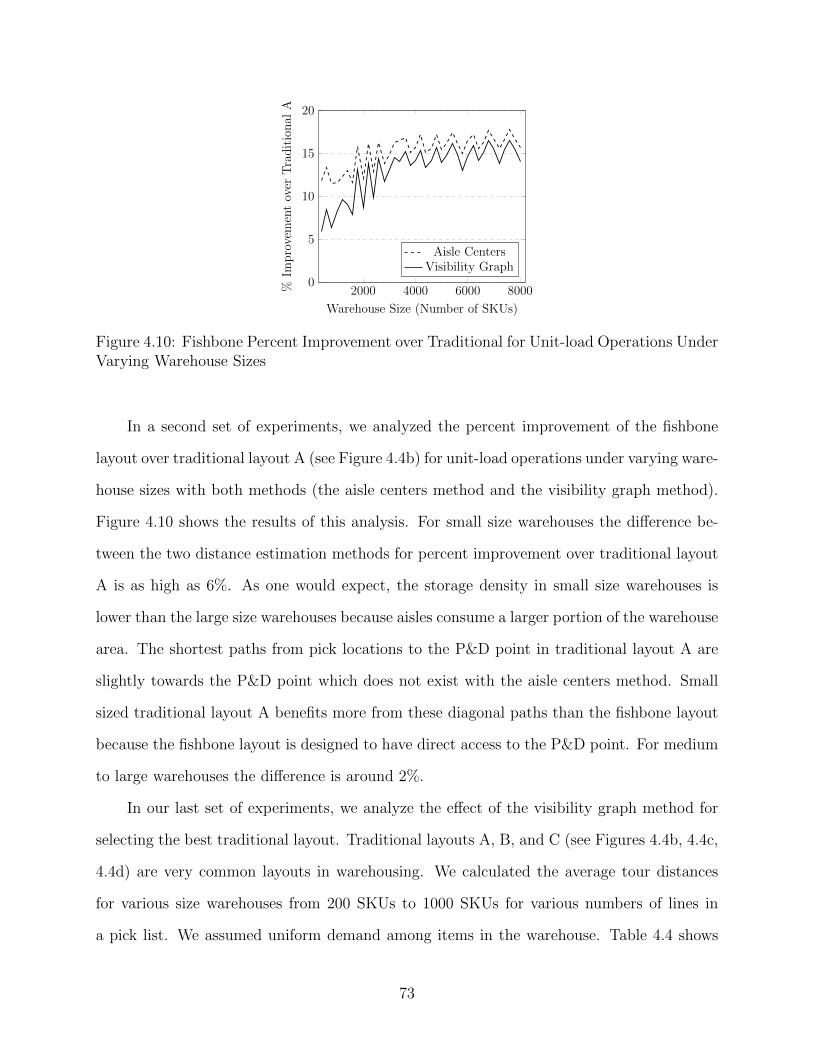
2000 4000 6000 80000

5

10

15

20

Warehouse Size (Number of SKUs)

%Im

pro

vem

ent

over

Tra

dit

ional

A

Aisle CentersVisibility Graph

Figure 4.10: Fishbone Percent Improvement over Traditional for Unit-load Operations UnderVarying Warehouse Sizes

In a second set of experiments, we analyzed the percent improvement of the fishbone

layout over traditional layout A (see Figure 4.4b) for unit-load operations under varying ware-

house sizes with both methods (the aisle centers method and the visibility graph method).

Figure 4.10 shows the results of this analysis. For small size warehouses the difference be-

tween the two distance estimation methods for percent improvement over traditional layout

A is as high as 6%. As one would expect, the storage density in small size warehouses is

lower than the large size warehouses because aisles consume a larger portion of the warehouse

area. The shortest paths from pick locations to the P&D point in traditional layout A are

slightly towards the P&D point which does not exist with the aisle centers method. Small

sized traditional layout A benefits more from these diagonal paths than the fishbone layout

because the fishbone layout is designed to have direct access to the P&D point. For medium

to large warehouses the difference is around 2%.

In our last set of experiments, we analyze the effect of the visibility graph method for

selecting the best traditional layout. Traditional layouts A, B, and C (see Figures 4.4b, 4.4c,

4.4d) are very common layouts in warehousing. We calculated the average tour distances

for various size warehouses from 200 SKUs to 1000 SKUs for various numbers of lines in

a pick list. We assumed uniform demand among items in the warehouse. Table 4.4 shows

73

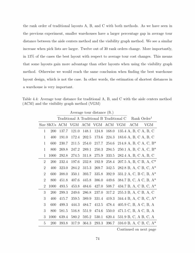
the rank order of traditional layouts A, B, and C with both methods. As we have seen in

the previous experiment, smaller warehouses have a larger percentage gap in average tour

distance between the aisle centers method and the visibility graph method. We see a similar

increase when pick lists are larger. Twelve out of 30 rank orders change. More importantly,

in 13% of the cases the best layout with respect to average tour cost changes. This means

that some layouts gain more advantage than other layouts when using the visibility graph

method. Otherwise we would reach the same conclusion when finding the best warehouse

layout design, which is not the case. In other words, the estimation of shortest distances in

a warehouse is very important.

Table 4.4: Average tour distance for traditional A, B, and C with the aisle centers method(ACM) and the visibility graph method (VGM)

Average tour distance (ft.)

Traditional A Traditional B Traditional C Rank Order1

Size SKUs ACM VGM ACM VGM ACM VGM ACM VGM

1 200 137.7 121.0 148.1 124.8 168.0 135.4 A, B, C A, B, C

1 400 191.0 172.4 202.5 173.6 224.3 183.6 A, B, C A, B, C

1 600 230.7 211.5 254.0 217.7 254.6 214.8 A, B, C A, C, B*

1 800 269.8 247.2 289.1 250.3 294.5 250.1 A, B, C A, C, B*

1 1000 292.8 274.5 311.8 275.9 333.5 282.4 A, B, C A, B, C

2 200 232.4 197.6 232.8 192.9 258.4 207.5 A, B, C B, A, C*

2 400 323.0 284.2 315.3 269.7 342.5 282.8 B, A, C B, C, A*

2 600 388.0 350.1 393.7 335.8 392.9 331.2 A, C, B C, B, A*

2 800 451.8 407.6 445.8 386.0 449.6 384.7 B, C, A C, B, A*

2 1000 493.5 453.8 484.6 427.0 508.7 434.7 B, A, C B, C, A*

3 200 299.3 249.6 286.8 237.0 317.2 255.3 B, A, C B, A, C

3 400 415.7 359.5 389.9 331.4 419.3 344.4 B, A, C B, C, A*

3 600 499.3 444.3 484.7 412.5 478.4 405.9 C, B, A C, B, A

3 800 581.5 516.8 551.9 474.6 550.0 471.5 C, B, A C, B, A

3 1000 639.4 580.2 595.2 530.1 620.4 531.9 B, C, A B, C, A

5 200 393.8 317.9 364.3 293.3 396.7 316.0 B, A, C B, C, A*

Continued on next page

74

Table 4.4 – continued from previous page

Average tour distance (ft.)

Traditional A Traditional B Traditional C Rank Order1

Size SKUs ACM VGM ACM VGM ACM VGM ACM VGM

5 400 547.2 464.3 495.9 412.8 524.8 427.9 B, C, A B, C, A

5 600 665.2 575.1 615.1 517.3 602.2 501.6 C, B, A C, B, A

5 800 775.5 672.9 702.4 597.2 686.7 585.3 C, B, A C, B, A

5 1000 848.4 754.7 760.2 662.9 777.3 661.0 B, C, A C, B, A*

10 200 542.1 426.9 494.8 380.8 523.8 404.6 B, C, A B, C, A

10 400 777.2 634.1 681.3 548.4 698.9 553.6 B, C, A B, C, A

10 600 951.4 797.9 845.5 683.5 799.3 653.3 C, B, A C, B, A

10 800 1121.7 943.1 972.2 795.0 919.0 760.0 C, B, A C, B, A

10 1000 1235.0 1070.9 1052.4 885.6 1033.2 858.7 C, B, A C, B, A

30 200 764.4 610.2 740.8 549.7 807.3 593.9 B, A, C B, C, A*

30 400 1189.0 969.2 1105.2 838.1 1119.2 837.2 B, C, A C, B, A*

30 600 1528.9 1271.9 1400.5 1074.6 1300.7 1006.7 C, B, A C, B, A

30 800 1873.6 1538.8 1655.3 1271.8 1508.4 1179.1 C, B, A C, B, A

30 1000 2096.6 1801.0 1808.9 1432.9 1722.4 1343.8 C, B, A C, B, A

4.5 Conclusion

In conclusion, the visibility graph method affects the previous results of Gue and Meller

(2009) and Celik and Sural (2014). First, the performance improvements of the fishbone

layout varies from the aisle centers method as much as 9%. Second, the visibility graph

method has a larger impact for small size warehouses when comparing the fishbone layout to

the traditional layout. This indicates the importance of a good distance estimation for order

picking operations. Third, it also affects the best layout selection in a traditional layout

setting.

1(*) indicates that the rank order has changed

75

Chapter 5

A Computational System to Solve the Warehouse Aisle Design Problem

5.1 Introduction

Order picking is the most costly operation in a warehouse. However, current warehouse

design practices have been using the same design principles for more than sixty years: straight

rows with parallel pick aisles and perpendicular cross aisles that reduce the travel distance

between pick locations (Vaughan and Petersen, 1999; Petersen, 1999). Gue and Meller (2009)

recently challenged these assumptions by proposing the fishbone layout, which achieved

reductions in travel distance up to 20% in unit-load warehouses. The fishbone layout has

been effectively applied to newly built warehouses (Meller and Gue, 2009). Warehouses that

are already constructed may also get a high return on investment with a warehouse re-design

if there is a highly increased efficiency in order picking operations. Berglund and Batta

(2012) state that cross aisle configurations may be changed without incurring prohibitive

costs. Some order picking operations are performed by picking from a pallet storage which

can be easily reconfigured to re-orient the cross aisle and pick aisle positions.

Dukic and Opetuk (2008) and Celik and Sural (2014) analyze the fishbone layout for

order picking operations with different routing policies and show that the fishbone layout can

perform as much as 30% worse than a traditional layout. However, the research in finding

optimal layouts for order picking warehouses is lacking. The main result of this paper is to

show that there are non-traditional designs that reduce the cost of order picking operation

by changing the aisle orientation, aspect ratio, and placement of depot simultaneously.

76

5%Other

10%Setup

15%Pick

20%Search

50%Travel

0% 20% 40% 60%percent of order pickers time

Figure 5.1: Typical distribution of an order picker’s time (Tompkins, 2010)

5.2 Literature Review

Order picking is the retrieval of items from a storage area to fulfill customer orders. It

involves the process of grouping and scheduling customer orders, releasing them to the order

pickers, picking of the items from storage locations, and the disposal of the picked items

(De Koster et al., 2007). The faster an order can be retrieved, the sooner it is available for

shipping to the customer. Therefore, minimizing order retrieval time is a key to a successful

warehouse. Figure 5.1 shows the order picking time components in a typical warehouse. 50%

of the order picker’s time is travel time. For manual-pick order picking systems, travel time

is an increasing function of the travel distance (De Koster et al., 2007). For these reasons,

we select minimizing travel distance as an objective for improvement.

Warehouses can have multiple order picking systems. These systems are either manual

or automated. Tompkins (2010) states that there must be a balance between the level of

automated systems (which are inflexible) and labor in order to respond to future business

requirements without sacrificing logical labor savings today. Because automation is capital

intensive and inflexible, the majority of warehouses employ humans for order picking (Le-

Duc, 2005). In this paper we limit ourselves to low-level picker-to-parts systems with multiple

picks per route. In these systems, an order picker picks items from bin shelving storage, pallet

storage on the floor, modular storage drawers/cabinets, or gravity flow racks. Cart picking

77

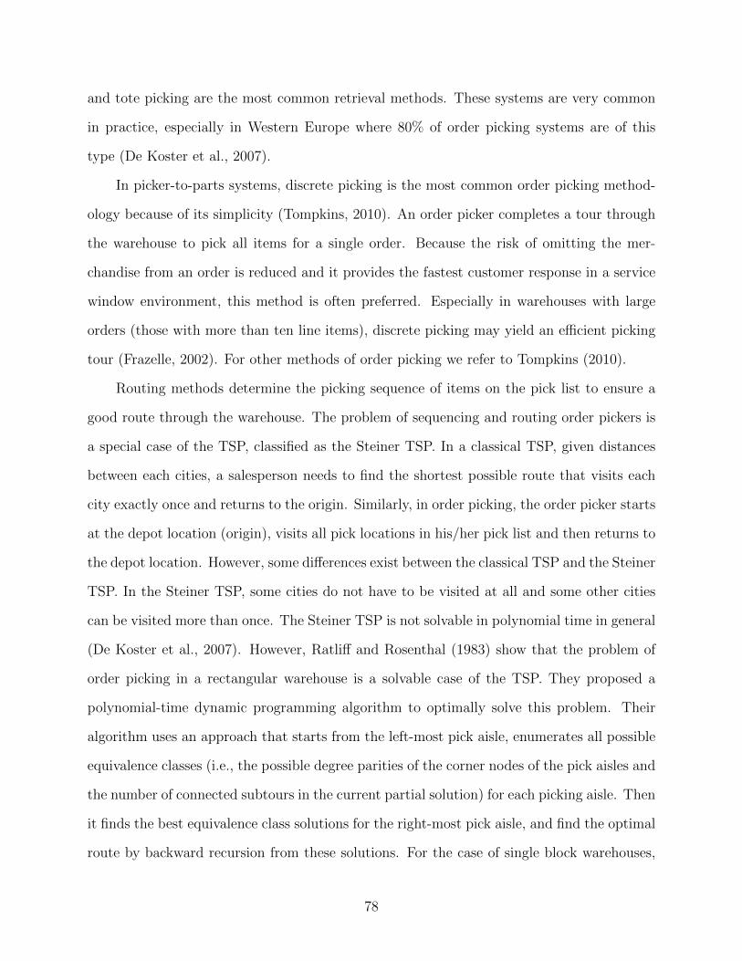
and tote picking are the most common retrieval methods. These systems are very common

in practice, especially in Western Europe where 80% of order picking systems are of this

type (De Koster et al., 2007).

In picker-to-parts systems, discrete picking is the most common order picking method-

ology because of its simplicity (Tompkins, 2010). An order picker completes a tour through

the warehouse to pick all items for a single order. Because the risk of omitting the mer-

chandise from an order is reduced and it provides the fastest customer response in a service

window environment, this method is often preferred. Especially in warehouses with large

orders (those with more than ten line items), discrete picking may yield an efficient picking

tour (Frazelle, 2002). For other methods of order picking we refer to Tompkins (2010).

Routing methods determine the picking sequence of items on the pick list to ensure a

good route through the warehouse. The problem of sequencing and routing order pickers is

a special case of the TSP, classified as the Steiner TSP. In a classical TSP, given distances

between each cities, a salesperson needs to find the shortest possible route that visits each

city exactly once and returns to the origin. Similarly, in order picking, the order picker starts

at the depot location (origin), visits all pick locations in his/her pick list and then returns to

the depot location. However, some differences exist between the classical TSP and the Steiner

TSP. In the Steiner TSP, some cities do not have to be visited at all and some other cities

can be visited more than once. The Steiner TSP is not solvable in polynomial time in general

(De Koster et al., 2007). However, Ratliff and Rosenthal (1983) show that the problem of

order picking in a rectangular warehouse is a solvable case of the TSP. They proposed a

polynomial-time dynamic programming algorithm to optimally solve this problem. Their

algorithm uses an approach that starts from the left-most pick aisle, enumerates all possible

equivalence classes (i.e., the possible degree parities of the corner nodes of the pick aisles and

the number of connected subtours in the current partial solution) for each picking aisle. Then

it finds the best equivalence class solutions for the right-most pick aisle, and find the optimal

route by backward recursion from these solutions. For the case of single block warehouses,

78

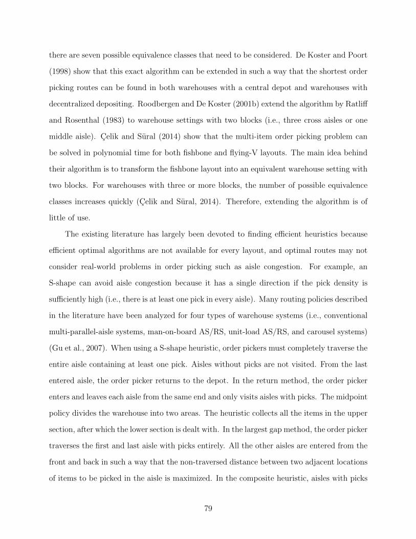
there are seven possible equivalence classes that need to be considered. De Koster and Poort

(1998) show that this exact algorithm can be extended in such a way that the shortest order

picking routes can be found in both warehouses with a central depot and warehouses with

decentralized depositing. Roodbergen and De Koster (2001b) extend the algorithm by Ratliff

and Rosenthal (1983) to warehouse settings with two blocks (i.e., three cross aisles or one

middle aisle). Celik and Sural (2014) show that the multi-item order picking problem can

be solved in polynomial time for both fishbone and flying-V layouts. The main idea behind

their algorithm is to transform the fishbone layout into an equivalent warehouse setting with

two blocks. For warehouses with three or more blocks, the number of possible equivalence

classes increases quickly (Celik and Sural, 2014). Therefore, extending the algorithm is of

little of use.

The existing literature has largely been devoted to finding efficient heuristics because

efficient optimal algorithms are not available for every layout, and optimal routes may not

consider real-world problems in order picking such as aisle congestion. For example, an

S-shape can avoid aisle congestion because it has a single direction if the pick density is

sufficiently high (i.e., there is at least one pick in every aisle). Many routing policies described

in the literature have been analyzed for four types of warehouse systems (i.e., conventional

multi-parallel-aisle systems, man-on-board AS/RS, unit-load AS/RS, and carousel systems)

(Gu et al., 2007). When using a S-shape heuristic, order pickers must completely traverse the

entire aisle containing at least one pick. Aisles without picks are not visited. From the last

entered aisle, the order picker returns to the depot. In the return method, the order picker

enters and leaves each aisle from the same end and only visits aisles with picks. The midpoint

policy divides the warehouse into two areas. The heuristic collects all the items in the upper

section, after which the lower section is dealt with. In the largest gap method, the order picker

traverses the first and last aisle with picks entirely. All the other aisles are entered from the

front and back in such a way that the non-traversed distance between two adjacent locations

of items to be picked in the aisle is maximized. In the composite heuristic, aisles with picks

79

are visited, but dynamic programming is used to decide either entirely traverse or enter and

left at the same end (see Roodbergen and De Koster (2001a)). Petersen (1997) analyzes

six routing heuristics (S-shape, return, midpoint, largest gap, composite, and optimal) for

single-block warehouses and concludes that the best heuristic solution is on average 5% more

than the optimal solution.

These routing heuristics are not suitable for our research for two reasons. First, these

heuristics are designed for single-block warehouses and some (aisle-by-aisle, S-shape, largest

gap, combined) can be modified for multiple-block warehouses, but they are not designed

for non-traditional designs. Therefore, the routing might not work in some non-traditional

designs. Second and most important, these heuristics are fairly simple construction heuristics

which construct a feasible solution, without attempting any improvement by means of local

search or meta-heuristic search.

Makris and Giakoumakis (2003) present Lin and Kernighan (1973)s TSP-based k-

interchange methodology for single-block warehouses and show that their procedure out-

performed the S-shape heuristic in seven of eleven examined cases. Theys et al. (2010)

extend their research for multi-block warehouses and achieve average savings in route dis-

tance of up to 47% when using the Lin-Kerhighan-Helsgaun (LKH) heuristic (Helsgaun,

2000) compared to S-shape, largest gap, combined, and aisle-by-aisle heuristics. The quality

of the solutions by the LKH heuristic is, on average, clearly superior to the other routing

heuristics. Although the LKH heuristic’s average computation time (0.25 seconds) is more

than these heuristics (the calculation time is negligible for these heuristics) it is 36 times

faster than the exact TSP algorithm “Concorde” (9.23 seconds). Moreover, LKH’s solutions

deviate on average only 0.1% from optimum. Therefore, we select LKH as our routing algo-

rithm. A detailed description of these routing policies and their variations can be found in

De Koster et al. (2007), Gu et al. (2007), and Helsgaun (2000).

80

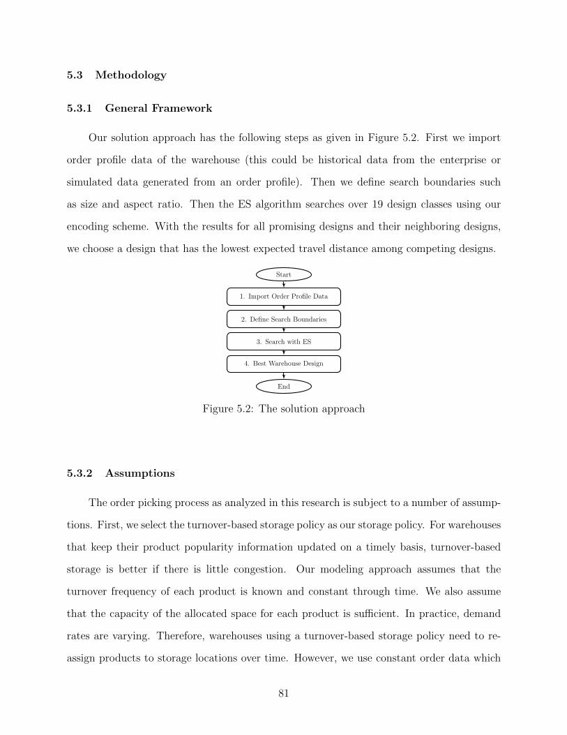
5.3 Methodology

5.3.1 General Framework

Our solution approach has the following steps as given in Figure 5.2. First we import

order profile data of the warehouse (this could be historical data from the enterprise or

simulated data generated from an order profile). Then we define search boundaries such

as size and aspect ratio. Then the ES algorithm searches over 19 design classes using our

encoding scheme. With the results for all promising designs and their neighboring designs,

we choose a design that has the lowest expected travel distance among competing designs.

Start

1. Import Order Profile Data

2. Define Search Boundaries

3. Search with ES

4. Best Warehouse Design

End

Figure 5.2: The solution approach

5.3.2 Assumptions

The order picking process as analyzed in this research is subject to a number of assump-

tions. First, we select the turnover-based storage policy as our storage policy. For warehouses

that keep their product popularity information updated on a timely basis, turnover-based

storage is better if there is little congestion. Our modeling approach assumes that the

turnover frequency of each product is known and constant through time. We also assume

that the capacity of the allocated space for each product is sufficient. In practice, demand

rates are varying. Therefore, warehouses using a turnover-based storage policy need to re-

assign products to storage locations over time. However, we use constant order data which

81

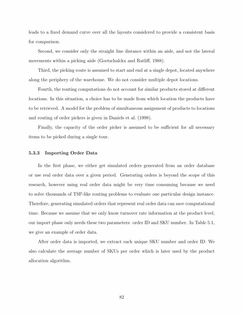
leads to a fixed demand curve over all the layouts considered to provide a consistent basis

for comparison.

Second, we consider only the straight line distance within an aisle, and not the lateral

movements within a picking aisle (Goetschalckx and Ratliff, 1988).

Third, the picking route is assumed to start and end at a single depot, located anywhere

along the periphery of the warehouse. We do not consider multiple depot locations.

Fourth, the routing computations do not account for similar products stored at different

locations. In this situation, a choice has to be made from which location the products have

to be retrieved. A model for the problem of simultaneous assignment of products to locations

and routing of order pickers is given in Daniels et al. (1998).

Finally, the capacity of the order picker is assumed to be sufficient for all necessary

items to be picked during a single tour.

5.3.3 Importing Order Data

In the first phase, we either get simulated orders generated from an order database

or use real order data over a given period. Generating orders is beyond the scope of this

research, however using real order data might be very time consuming because we need

to solve thousands of TSP-like routing problems to evaluate one particular design instance.

Therefore, generating simulated orders that represent real order data can save computational

time. Because we assume that we only know turnover rate information at the product level,

our import phase only needs these two parameters: order ID and SKU number. In Table 5.1,

we give an example of order data.

After order data is imported, we extract each unique SKU number and order ID. We

also calculate the average number of SKUs per order which is later used by the product

allocation algorithm.

82

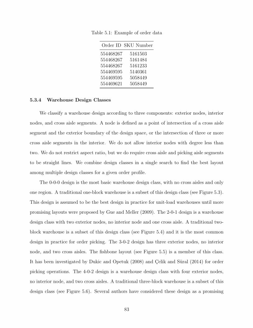
Table 5.1: Example of order data

Order ID SKU Number

554468267 5161503554468267 5161484554468267 5161233554469595 5140361554469595 5058449554469621 5058449

5.3.4 Warehouse Design Classes

We classify a warehouse design according to three components: exterior nodes, interior

nodes, and cross aisle segments. A node is defined as a point of intersection of a cross aisle

segment and the exterior boundary of the design space, or the intersection of three or more

cross aisle segments in the interior. We do not allow interior nodes with degree less than

two. We do not restrict aspect ratio, but we do require cross aisle and picking aisle segments

to be straight lines. We combine design classes in a single search to find the best layout

among multiple design classes for a given order profile.

The 0-0-0 design is the most basic warehouse design class, with no cross aisles and only

one region. A traditional one-block warehouse is a subset of this design class (see Figure 5.3).

This design is assumed to be the best design in practice for unit-load warehouses until more

promising layouts were proposed by Gue and Meller (2009). The 2-0-1 design is a warehouse

design class with two exterior nodes, no interior node and one cross aisle. A traditional two-

block warehouse is a subset of this design class (see Figure 5.4) and it is the most common

design in practice for order picking. The 3-0-2 design has three exterior nodes, no interior

node, and two cross aisles. The fishbone layout (see Figure 5.5) is a member of this class.

It has been investigated by Dukic and Opetuk (2008) and Celik and Sural (2014) for order

picking operations. The 4-0-2 design is a warehouse design class with four exterior nodes,

no interior node, and two cross aisles. A traditional three-block warehouse is a subset of this

design class (see Figure 5.6). Several authors have considered these design as a promising

83

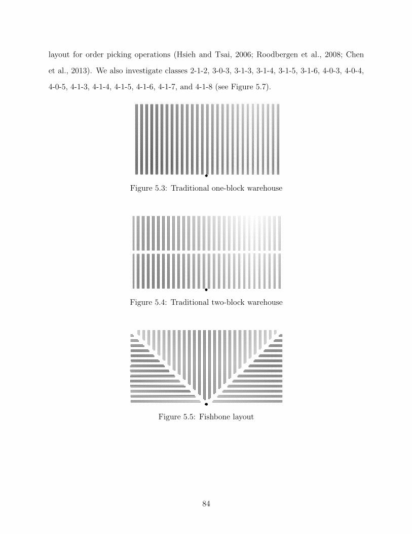
layout for order picking operations (Hsieh and Tsai, 2006; Roodbergen et al., 2008; Chen

et al., 2013). We also investigate classes 2-1-2, 3-0-3, 3-1-3, 3-1-4, 3-1-5, 3-1-6, 4-0-3, 4-0-4,

4-0-5, 4-1-3, 4-1-4, 4-1-5, 4-1-6, 4-1-7, and 4-1-8 (see Figure 5.7).

Figure 5.3: Traditional one-block warehouse

Figure 5.4: Traditional two-block warehouse

Figure 5.5: Fishbone layout

84

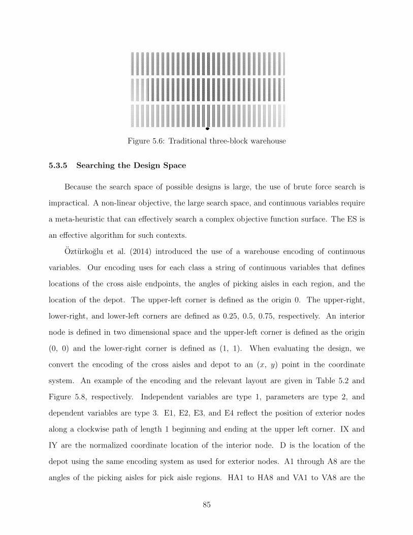
Figure 5.6: Traditional three-block warehouse

5.3.5 Searching the Design Space

Because the search space of possible designs is large, the use of brute force search is

impractical. A non-linear objective, the large search space, and continuous variables require

a meta-heuristic that can effectively search a complex objective function surface. The ES is

an effective algorithm for such contexts.

Ozturkoglu et al. (2014) introduced the use of a warehouse encoding of continuous

variables. Our encoding uses for each class a string of continuous variables that defines

locations of the cross aisle endpoints, the angles of picking aisles in each region, and the

location of the depot. The upper-left corner is defined as the origin 0. The upper-right,

lower-right, and lower-left corners are defined as 0.25, 0.5, 0.75, respectively. An interior

node is defined in two dimensional space and the upper-left corner is defined as the origin

(0, 0) and the lower-right corner is defined as (1, 1). When evaluating the design, we

convert the encoding of the cross aisles and depot to an (x, y) point in the coordinate

system. An example of the encoding and the relevant layout are given in Table 5.2 and

Figure 5.8, respectively. Independent variables are type 1, parameters are type 2, and

dependent variables are type 3. E1, E2, E3, and E4 reflect the position of exterior nodes

along a clockwise path of length 1 beginning and ending at the upper left corner. IX and

IY are the normalized coordinate location of the interior node. D is the location of the

depot using the same encoding system as used for exterior nodes. A1 through A8 are the

angles of the picking aisles for pick aisle regions. HA1 to HA8 and VA1 to VA8 are the

85

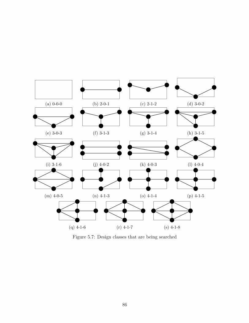
(a) 0-0-0 (b) 2-0-1 (c) 2-1-2 (d) 3-0-2

(e) 3-0-3 (f) 3-1-3 (g) 3-1-4 (h) 3-1-5

(i) 3-1-6 (j) 4-0-2 (k) 4-0-3 (l) 4-0-4

(m) 4-0-5 (n) 4-1-3 (o) 4-1-4 (p) 4-1-5

(q) 4-1-6 (r) 4-1-7 (s) 4-1-8

Figure 5.7: Design classes that are being searched

86

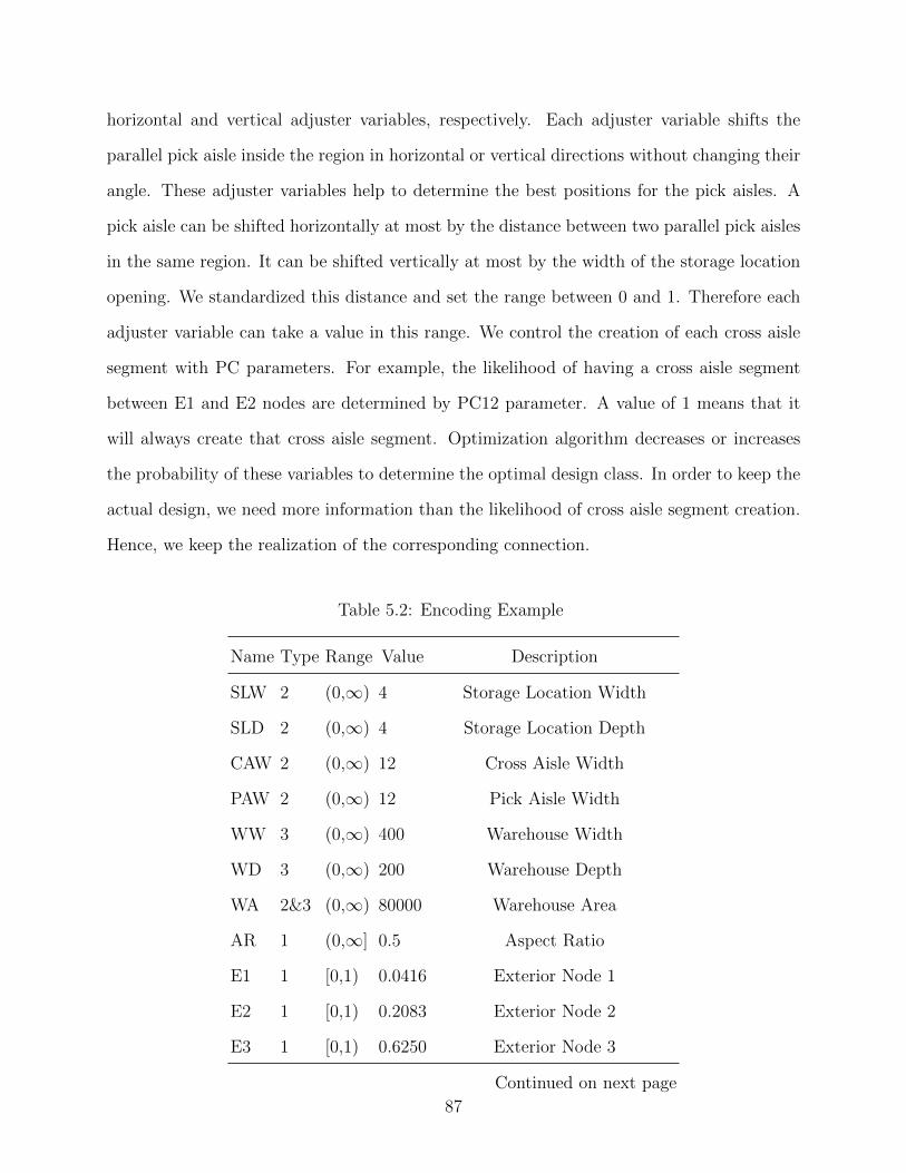
horizontal and vertical adjuster variables, respectively. Each adjuster variable shifts the

parallel pick aisle inside the region in horizontal or vertical directions without changing their

angle. These adjuster variables help to determine the best positions for the pick aisles. A

pick aisle can be shifted horizontally at most by the distance between two parallel pick aisles

in the same region. It can be shifted vertically at most by the width of the storage location

opening. We standardized this distance and set the range between 0 and 1. Therefore each

adjuster variable can take a value in this range. We control the creation of each cross aisle

segment with PC parameters. For example, the likelihood of having a cross aisle segment

between E1 and E2 nodes are determined by PC12 parameter. A value of 1 means that it

will always create that cross aisle segment. Optimization algorithm decreases or increases

the probability of these variables to determine the optimal design class. In order to keep the

actual design, we need more information than the likelihood of cross aisle segment creation.

Hence, we keep the realization of the corresponding connection.

Table 5.2: Encoding Example

Name Type Range Value Description

SLW 2 (0,∞) 4 Storage Location Width

SLD 2 (0,∞) 4 Storage Location Depth

CAW 2 (0,∞) 12 Cross Aisle Width

PAW 2 (0,∞) 12 Pick Aisle Width

WW 3 (0,∞) 400 Warehouse Width

WD 3 (0,∞) 200 Warehouse Depth

WA 2&3 (0,∞) 80000 Warehouse Area

AR 1 (0,∞] 0.5 Aspect Ratio

E1 1 [0,1) 0.0416 Exterior Node 1

E2 1 [0,1) 0.2083 Exterior Node 2

E3 1 [0,1) 0.6250 Exterior Node 3

Continued on next page

87

Table 5.2 – continued from previous page

Name Type Range Value Description

E4 1 [0,1) 0.6250 Exterior Node 4

IX 1 (0,1) 0.5000 Interior Node X Axis

IY 1 (0,1) 0.5000 Interior Node Y Axis

D 1 (0,1) 0.5 Depot

A1 1 [0,1) 0.1777 Region 1 Angle (32◦)

A2 1 [0,1) 0.8166 Region 2 Angle (147◦)

A3 1 [0,1) 0.5000 Region 3 Angle (90◦)

A4 1 [0,1) 0.5000 Region 4 Angle (90◦)

A5 1 [0,1) 0.5000 Region 5 Angle (90◦)

A6 1 [0,1) 0.5000 Region 6 Angle (90◦)

A7 1 [0,1) 0.5000 Region 7 Angle (90◦)

A8 1 [0,1) 0.5000 Region 8 Angle (90◦)

HA1 1 [0,1) 0.5000 Horizontal Adjuster 1

HA2 1 [0,1) 0.5000 Horizontal Adjuster 2

HA3 1 [0,1) 0.5000 Horizontal Adjuster 3

HA4 1 [0,1) 0.5000 Horizontal Adjuster 4

HA5 1 [0,1) 0.5000 Horizontal Adjuster 5

HA6 1 [0,1) 0.5000 Horizontal Adjuster 6

HA7 1 [0,1) 0.5000 Horizontal Adjuster 7

HA8 1 [0,1) 0.5000 Horizontal Adjuster 8

VA1 1 [0,1) 0.5000 Vertical Adjuster 1

VA2 1 [0,1) 0.5000 Vertical Adjuster 2

VA3 1 [0,1) 0.5000 Vertical Adjuster 3

VA4 1 [0,1) 0.5000 Vertical Adjuster 4

Continued on next page

88

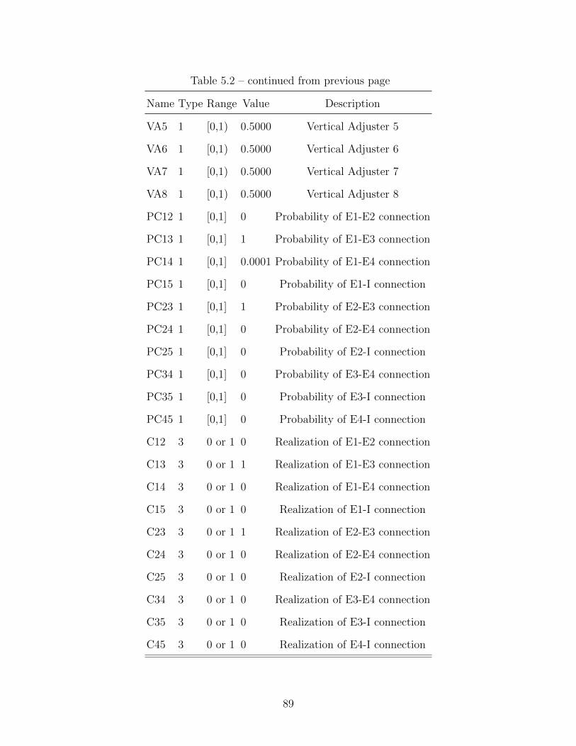
Table 5.2 – continued from previous page

Name Type Range Value Description

VA5 1 [0,1) 0.5000 Vertical Adjuster 5

VA6 1 [0,1) 0.5000 Vertical Adjuster 6

VA7 1 [0,1) 0.5000 Vertical Adjuster 7

VA8 1 [0,1) 0.5000 Vertical Adjuster 8

PC12 1 [0,1] 0 Probability of E1-E2 connection

PC13 1 [0,1] 1 Probability of E1-E3 connection

PC14 1 [0,1] 0.0001 Probability of E1-E4 connection

PC15 1 [0,1] 0 Probability of E1-I connection

PC23 1 [0,1] 1 Probability of E2-E3 connection

PC24 1 [0,1] 0 Probability of E2-E4 connection

PC25 1 [0,1] 0 Probability of E2-I connection

PC34 1 [0,1] 0 Probability of E3-E4 connection

PC35 1 [0,1] 0 Probability of E3-I connection

PC45 1 [0,1] 0 Probability of E4-I connection

C12 3 0 or 1 0 Realization of E1-E2 connection

C13 3 0 or 1 1 Realization of E1-E3 connection

C14 3 0 or 1 0 Realization of E1-E4 connection

C15 3 0 or 1 0 Realization of E1-I connection

C23 3 0 or 1 1 Realization of E2-E3 connection

C24 3 0 or 1 0 Realization of E2-E4 connection

C25 3 0 or 1 0 Realization of E2-I connection

C34 3 0 or 1 0 Realization of E3-E4 connection

C35 3 0 or 1 0 Realization of E3-I connection

C45 3 0 or 1 0 Realization of E4-I connection

89

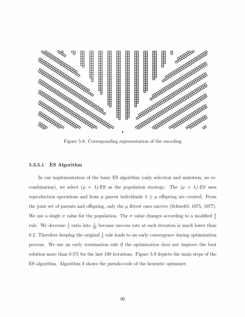
Figure 5.8: Corresponding representation of the encoding

5.3.5.1 ES Algorithm

In our implementation of the basic ES algorithm (only selection and mutation, no re-

combination), we select (µ + λ)-ES as the population strategy. The (µ + λ)-ES uses

reproduction operations and from µ parent individuals λ ≥ µ offspring are created. From

the joint set of parents and offspring, only the µ fittest ones survive (Schwefel, 1975, 1977).

We use a single σ value for the population. The σ value changes according to a modified 15

rule. We decrease 15

ratio into 120

because success rate at each iteration is much lower than

0.2. Therefore keeping the original 15

rule leads to an early convergence during optimization

process. We use an early termination rule if the optimization does not improve the best

solution more than 0.5% for the last 100 iterations. Figure 5.9 depicts the main steps of the

ES algorithm. Algorithm 3 shows the pseudo-code of the heuristic optimizer.

90

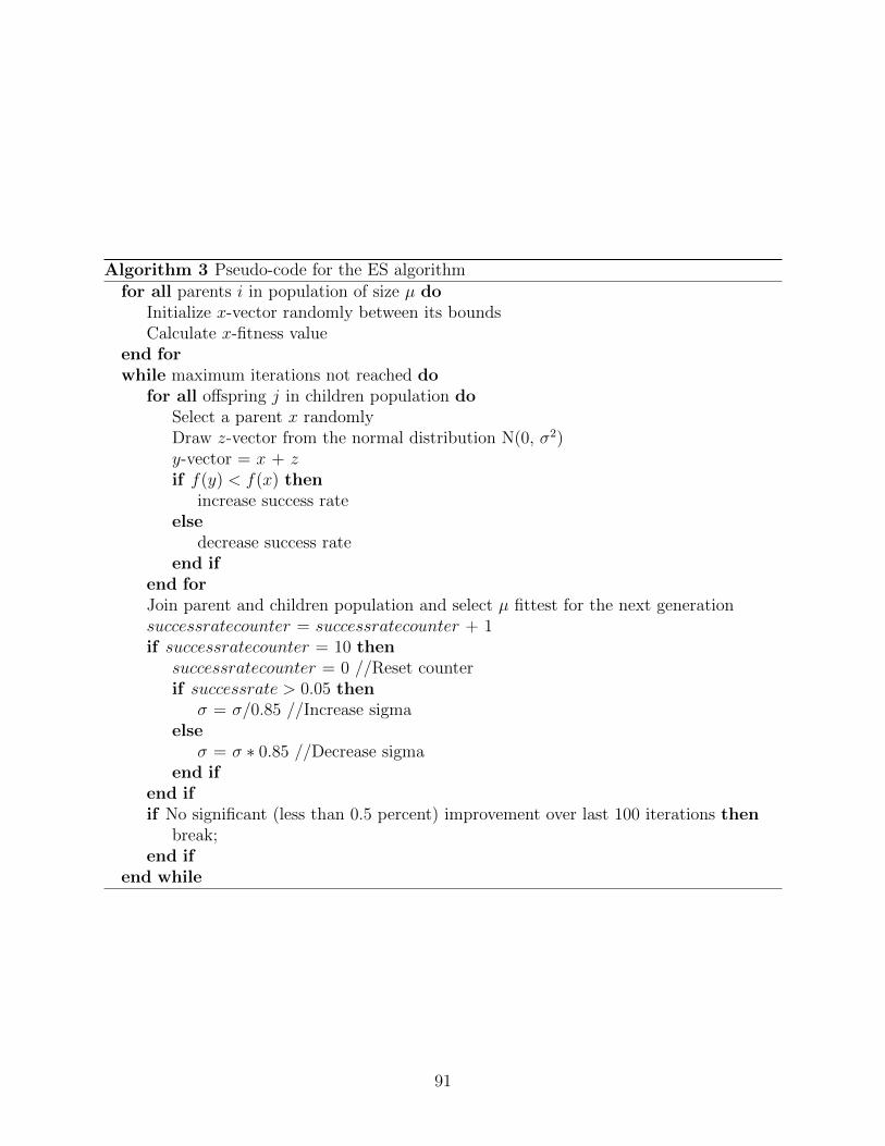
Algorithm 3 Pseudo-code for the ES algorithm

for all parents i in population of size µ doInitialize x-vector randomly between its boundsCalculate x-fitness value

end forwhile maximum iterations not reached do

for all offspring j in children population doSelect a parent x randomlyDraw z-vector from the normal distribution N(0, σ2)y-vector = x + zif f(y) < f(x) then

increase success rateelse

decrease success rateend if

end forJoin parent and children population and select µ fittest for the next generationsuccessratecounter = successratecounter + 1if successratecounter = 10 then

successratecounter = 0 //Reset counterif successrate > 0.05 then

σ = σ/0.85 //Increase sigmaelse

σ = σ ∗ 0.85 //Decrease sigmaend if

end ifif No significant (less than 0.5 percent) improvement over last 100 iterations then

break;end if

end while

91

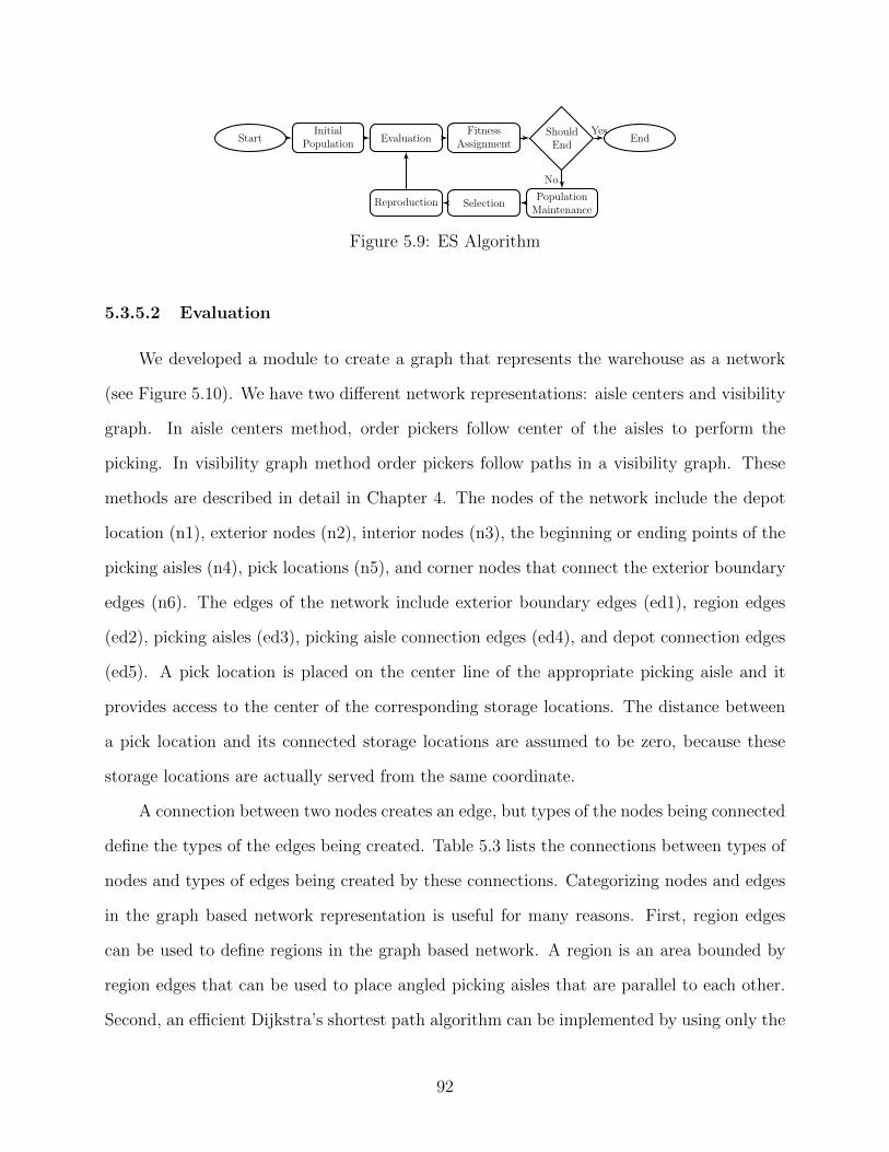
StartInitial

PopulationEvaluation

FitnessAssignment

ShouldEnd

PopulationMaintenance

SelectionReproduction

End

No

Yes

Figure 5.9: ES Algorithm

5.3.5.2 Evaluation

We developed a module to create a graph that represents the warehouse as a network

(see Figure 5.10). We have two different network representations: aisle centers and visibility

graph. In aisle centers method, order pickers follow center of the aisles to perform the

picking. In visibility graph method order pickers follow paths in a visibility graph. These

methods are described in detail in Chapter 4. The nodes of the network include the depot

location (n1), exterior nodes (n2), interior nodes (n3), the beginning or ending points of the

picking aisles (n4), pick locations (n5), and corner nodes that connect the exterior boundary

edges (n6). The edges of the network include exterior boundary edges (ed1), region edges

(ed2), picking aisles (ed3), picking aisle connection edges (ed4), and depot connection edges

(ed5). A pick location is placed on the center line of the appropriate picking aisle and it

provides access to the center of the corresponding storage locations. The distance between

a pick location and its connected storage locations are assumed to be zero, because these

storage locations are actually served from the same coordinate.

A connection between two nodes creates an edge, but types of the nodes being connected

define the types of the edges being created. Table 5.3 lists the connections between types of

nodes and types of edges being created by these connections. Categorizing nodes and edges

in the graph based network representation is useful for many reasons. First, region edges

can be used to define regions in the graph based network. A region is an area bounded by

region edges that can be used to place angled picking aisles that are parallel to each other.

Second, an efficient Dijkstra’s shortest path algorithm can be implemented by using only the

92

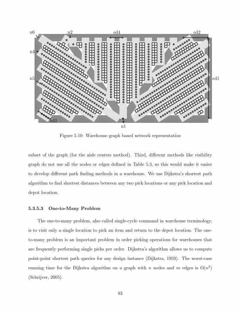
ed2ed4

ed1

n2

n4

n6

ed3n1

n5

Figure 5.10: Warehouse graph based network representation

subset of the graph (for the aisle centers method). Third, different methods like visibility

graph do not use all the nodes or edges defined in Table 5.3, so this would make it easier

to develop different path finding methods in a warehouse. We use Dijkstra’s shortest path

algorithm to find shortest distances between any two pick locations or any pick location and

depot location.

5.3.5.3 One-to-Many Problem

The one-to-many problem, also called single-cycle command in warehouse terminology,

is to visit only a single location to pick an item and return to the depot location. The one-

to-many problem is an important problem in order picking operations for warehouses that

are frequently performing single picks per order. Dijkstra’s algorithm allows us to compute

point-point shortest path queries for any design instance (Dijkstra, 1959). The worst-case

running time for the Dijkstra algorithm on a graph with n nodes and m edges is O(n2)

(Schrijver, 2005).

93

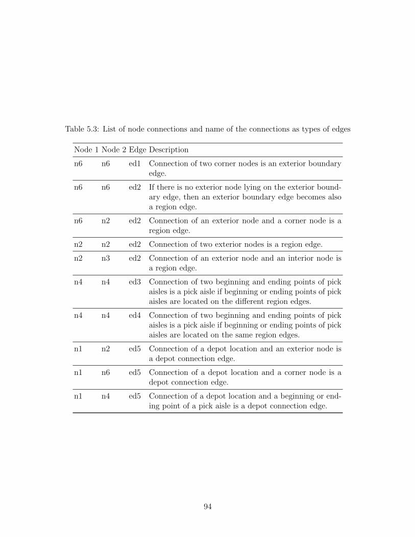
Table 5.3: List of node connections and name of the connections as types of edges

Node 1 Node 2 Edge Description

n6 n6 ed1 Connection of two corner nodes is an exterior boundaryedge.

n6 n6 ed2 If there is no exterior node lying on the exterior bound-ary edge, then an exterior boundary edge becomes alsoa region edge.

n6 n2 ed2 Connection of an exterior node and a corner node is aregion edge.

n2 n2 ed2 Connection of two exterior nodes is a region edge.

n2 n3 ed2 Connection of an exterior node and an interior node isa region edge.

n4 n4 ed3 Connection of two beginning and ending points of pickaisles is a pick aisle if beginning or ending points of pickaisles are located on the different region edges.

n4 n4 ed4 Connection of two beginning and ending points of pickaisles is a pick aisle if beginning or ending points of pickaisles are located on the same region edges.

n1 n2 ed5 Connection of a depot location and an exterior node isa depot connection edge.

n1 n6 ed5 Connection of a depot location and a corner node is adepot connection edge.

n1 n4 ed5 Connection of a depot location and a beginning or end-ing point of a pick aisle is a depot connection edge.

94

Figure 5.11: Single cycle command example

5.3.5.4 Many-to-Many Problem

The many-to-many problem, also called the many-to-many shortest path, is to calculate

the pick location to pick location shortest path distances to find locations that are closest

to any other location on average. In other words, by calculating many-to-many distances,

we find the pick locations that are close to the centroid of the design space. We still use

Dijkstra’s algorithm to calculate many-to-many distances. However, calculation of many-to-

many distances takes much more time compared to the calculation of one-to-many distances.

If we assume n is the total number of pick locations, the worst-case running time would be

O(n3). After calculating the total travel distances to every location for each location, we

sort the locations from minimum to maximum to find the most convenient locations for

multiple order picking operations. Algorithm 4 shows the details of all pairs shortest path

(i.e., many-to-many distances).

5.3.5.5 Storage (Product Allocation)

We select turnover-based as our storage policy. The most convenient locations for

multiple-command order picking for the turnover-based storage policy are not known in

the literature (Pohl et al., 2011). Therefore, we develop our own algorithm to allocate the

products to storage locations.

In the importing order data phase, we calculate the average order size. Because we

assume that the pick lists have been determined, each order picker travels through the

95

Algorithm 4 All-Pairs Shortest Path

function AllPairsShortestPath(void)for (i := 0;i < Count(G);i← i+ 1) do

DijkstrasShortestPath(G, i)end for

end function

function DijkstrasShortestPath(G, k) Q← ∅for (i := 0;i < Count(G);i← i+ 1) do

dist[k, i]←∞Add G[i] to Q

end fordist[k, k]← 0while Q is not empty do

u← min(Q)remove u from Qfor all v in neighbor of u do

shortdist← dist[k, u] + length(u, v)if shortdist < dist[k, v] then

dist[k, v]← shortdistend if

end forend while

end function

96

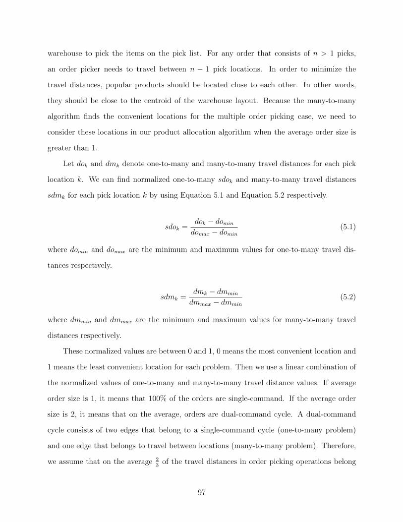
warehouse to pick the items on the pick list. For any order that consists of n > 1 picks,

an order picker needs to travel between n − 1 pick locations. In order to minimize the

travel distances, popular products should be located close to each other. In other words,

they should be close to the centroid of the warehouse layout. Because the many-to-many

algorithm finds the convenient locations for the multiple order picking case, we need to

consider these locations in our product allocation algorithm when the average order size is

greater than 1.

Let dok and dmk denote one-to-many and many-to-many travel distances for each pick

location k. We can find normalized one-to-many sdok and many-to-many travel distances

sdmk for each pick location k by using Equation 5.1 and Equation 5.2 respectively.

sdok =dok − domin

domax − domin

(5.1)

where domin and domax are the minimum and maximum values for one-to-many travel dis-

tances respectively.

sdmk =dmk − dmmin

dmmax − dmmin

(5.2)

where dmmin and dmmax are the minimum and maximum values for many-to-many travel

distances respectively.

These normalized values are between 0 and 1, 0 means the most convenient location and

1 means the least convenient location for each problem. Then we use a linear combination of

the normalized values of one-to-many and many-to-many travel distance values. If average

order size is 1, it means that 100% of the orders are single-command. If the average order

size is 2, it means that on the average, orders are dual-command cycle. A dual-command

cycle consists of two edges that belong to a single-command cycle (one-to-many problem)

and one edge that belongs to travel between locations (many-to-many problem). Therefore,

we assume that on the average 23

of the travel distances in order picking operations belong

97

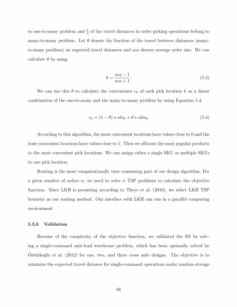
to one-to-many problem and 13

of the travel distances in order picking operations belong to

many-to-many problem. Let θ denote the fraction of the travel between distances (many-

to-many problem) on expected travel distances and aos denote average order size. We can

calculate θ by using:

θ =aos− 1

aos+ 1. (5.3)

We can use this θ to calculate the convenience ck of each pick location k as a linear

combination of the one-to-many and the many-to-many problem by using Equation 5.4:

ck = (1− θ) ∗ sdok + θ ∗ sdmk (5.4)

According to this algorithm, the most convenient locations have values close to 0 and the

least convenient locations have values close to 1. Then we allocate the most popular products

to the most convenient pick locations. We can assign either a single SKU or multiple SKUs

to one pick location.

Routing is the most computationally time consuming part of our design algorithm. For

a given number of orders n, we need to solve n TSP problems to calculate the objective

function. Since LKH is promising according to Theys et al. (2010), we select LKH TSP

heuristic as our routing method. Our interface with LKH can run in a parallel computing

environment.

5.3.6 Validation

Because of the complexity of the objective function, we validated the ES by solv-

ing a single-command unit-load warehouse problem, which has been optimally solved by

Ozturkoglu et al. (2012) for one, two, and three cross aisle designs. The objective is to

minimize the expected travel distance for single-command operations under random storage

98

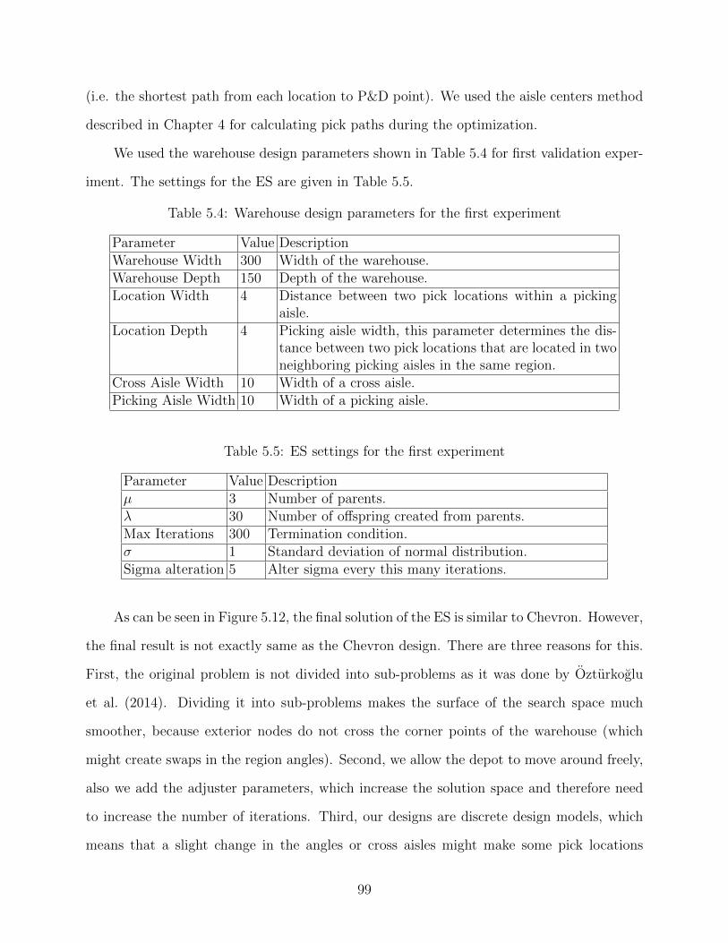
(i.e. the shortest path from each location to P&D point). We used the aisle centers method

described in Chapter 4 for calculating pick paths during the optimization.

We used the warehouse design parameters shown in Table 5.4 for first validation exper-

iment. The settings for the ES are given in Table 5.5.

Table 5.4: Warehouse design parameters for the first experiment

Parameter Value DescriptionWarehouse Width 300 Width of the warehouse.Warehouse Depth 150 Depth of the warehouse.Location Width 4 Distance between two pick locations within a picking

aisle.Location Depth 4 Picking aisle width, this parameter determines the dis-

tance between two pick locations that are located in twoneighboring picking aisles in the same region.

Cross Aisle Width 10 Width of a cross aisle.Picking Aisle Width 10 Width of a picking aisle.

Table 5.5: ES settings for the first experiment

Parameter Value Descriptionµ 3 Number of parents.λ 30 Number of offspring created from parents.Max Iterations 300 Termination condition.σ 1 Standard deviation of normal distribution.Sigma alteration 5 Alter sigma every this many iterations.

As can be seen in Figure 5.12, the final solution of the ES is similar to Chevron. However,

the final result is not exactly same as the Chevron design. There are three reasons for this.

First, the original problem is not divided into sub-problems as it was done by Ozturkoglu

et al. (2014). Dividing it into sub-problems makes the surface of the search space much

smoother, because exterior nodes do not cross the corner points of the warehouse (which

might create swaps in the region angles). Second, we allow the depot to move around freely,

also we add the adjuster parameters, which increase the solution space and therefore need

to increase the number of iterations. Third, our designs are discrete design models, which

means that a slight change in the angles or cross aisles might make some pick locations

99

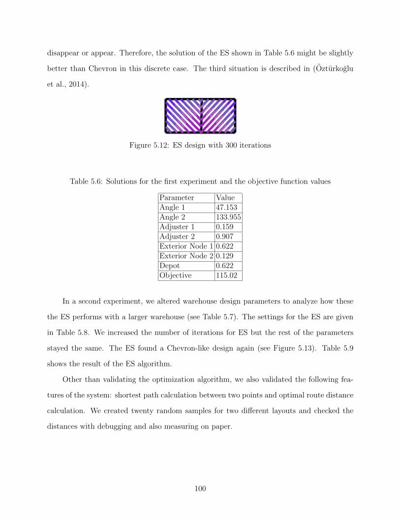
disappear or appear. Therefore, the solution of the ES shown in Table 5.6 might be slightly

better than Chevron in this discrete case. The third situation is described in (Ozturkoglu

et al., 2014).

Figure 5.12: ES design with 300 iterations

Table 5.6: Solutions for the first experiment and the objective function values

Parameter ValueAngle 1 47.153Angle 2 133.955Adjuster 1 0.159Adjuster 2 0.907Exterior Node 1 0.622Exterior Node 2 0.129Depot 0.622Objective 115.02

In a second experiment, we altered warehouse design parameters to analyze how these

the ES performs with a larger warehouse (see Table 5.7). The settings for the ES are given

in Table 5.8. We increased the number of iterations for ES but the rest of the parameters

stayed the same. The ES found a Chevron-like design again (see Figure 5.13). Table 5.9

shows the result of the ES algorithm.

Other than validating the optimization algorithm, we also validated the following fea-

tures of the system: shortest path calculation between two points and optimal route distance

calculation. We created twenty random samples for two different layouts and checked the

distances with debugging and also measuring on paper.

100

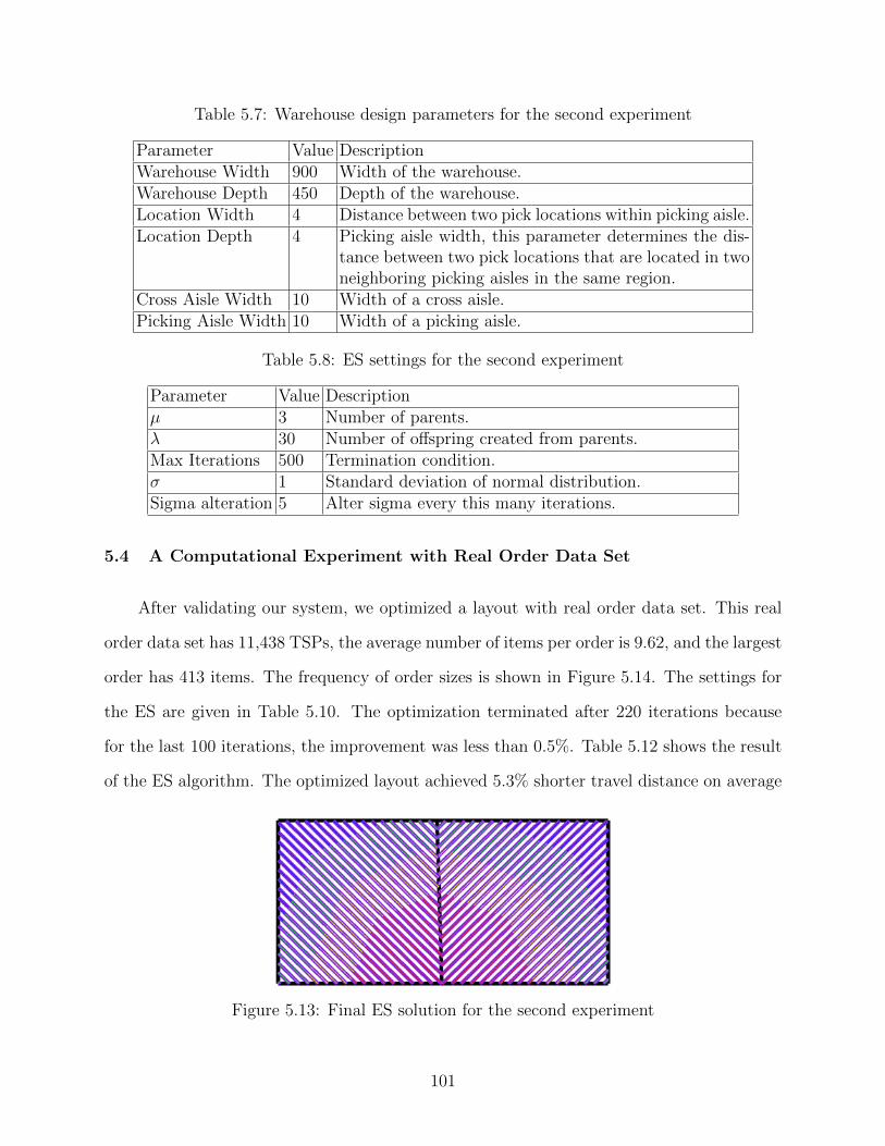
Table 5.7: Warehouse design parameters for the second experiment

Parameter Value DescriptionWarehouse Width 900 Width of the warehouse.Warehouse Depth 450 Depth of the warehouse.Location Width 4 Distance between two pick locations within picking aisle.Location Depth 4 Picking aisle width, this parameter determines the dis-

tance between two pick locations that are located in twoneighboring picking aisles in the same region.

Cross Aisle Width 10 Width of a cross aisle.Picking Aisle Width 10 Width of a picking aisle.

Table 5.8: ES settings for the second experiment

Parameter Value Descriptionµ 3 Number of parents.λ 30 Number of offspring created from parents.Max Iterations 500 Termination condition.σ 1 Standard deviation of normal distribution.Sigma alteration 5 Alter sigma every this many iterations.

5.4 A Computational Experiment with Real Order Data Set

After validating our system, we optimized a layout with real order data set. This real

order data set has 11,438 TSPs, the average number of items per order is 9.62, and the largest

order has 413 items. The frequency of order sizes is shown in Figure 5.14. The settings for

the ES are given in Table 5.10. The optimization terminated after 220 iterations because

for the last 100 iterations, the improvement was less than 0.5%. Table 5.12 shows the result

of the ES algorithm. The optimized layout achieved 5.3% shorter travel distance on average

Figure 5.13: Final ES solution for the second experiment

101

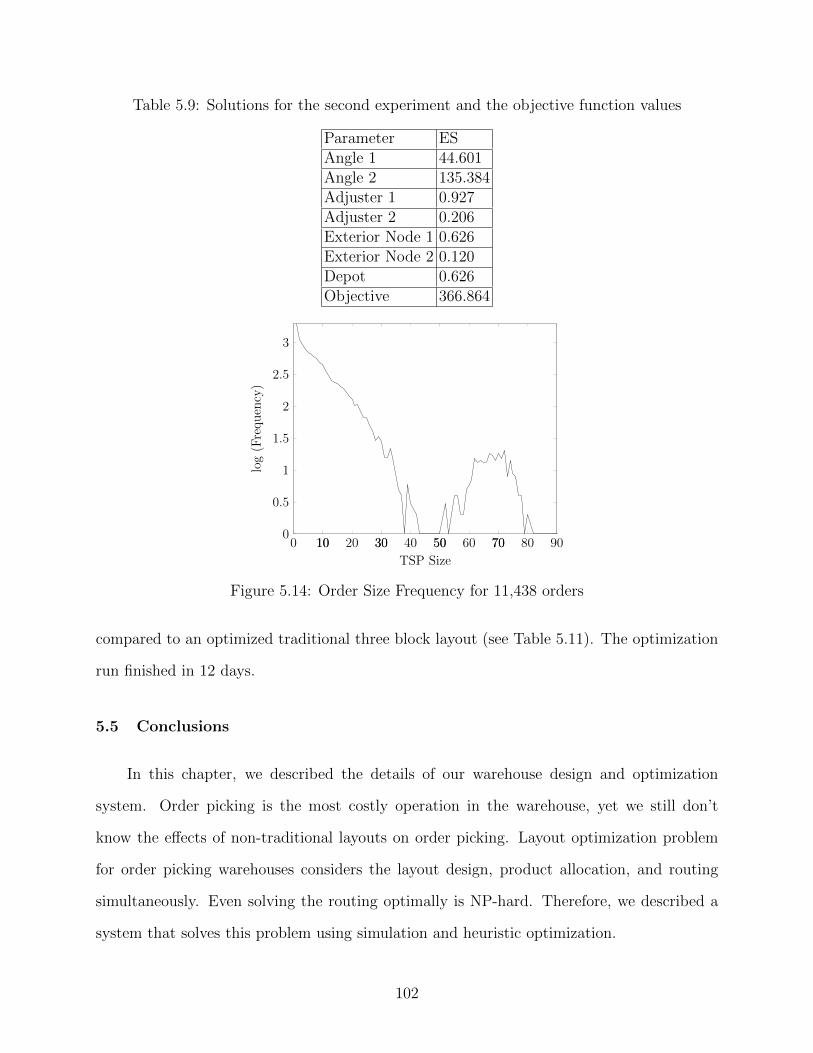
Table 5.9: Solutions for the second experiment and the objective function values

Parameter ESAngle 1 44.601Angle 2 135.384Adjuster 1 0.927Adjuster 2 0.206Exterior Node 1 0.626Exterior Node 2 0.120Depot 0.626Objective 366.864

0 10 20 30 40 50 60 70 80 900

0.5

1

1.5

2

2.5

3

10 30 50 70

TSP Size

log

(Fre

qu

ency

)

Figure 5.14: Order Size Frequency for 11,438 orders

compared to an optimized traditional three block layout (see Table 5.11). The optimization

run finished in 12 days.

5.5 Conclusions

In this chapter, we described the details of our warehouse design and optimization

system. Order picking is the most costly operation in the warehouse, yet we still don’t

know the effects of non-traditional layouts on order picking. Layout optimization problem

for order picking warehouses considers the layout design, product allocation, and routing

simultaneously. Even solving the routing optimally is NP-hard. Therefore, we described a

system that solves this problem using simulation and heuristic optimization.

102

Table 5.10: ES settings for the real order data experiment

Parameter Value Descriptionµ 20 Number of parents.λ 120 Number of offspring created from parents.Max Iterations 500 Termination condition.σ 0.5 Standard deviation of normal distribution.Sigma alteration 10 Alter sigma every this many iterations.

Table 5.11: Best Traditional Layout with Real Order Data

Parameter Value Design

Avg. PL Size 9.62E1, E2, E3, E4 0.041, 0.630, 0.921, 0.651IX, IY N/ADepot 0.625Angles 90, 90, 90# Locations 2622Aspect Ratio 0.8Width 412.90Depth 330.31Area 136386.22H.Adjusters 0.5, 0.5, 0.5V. Adjusters 0.5, 0.5, 0.5Avg. Travel Cost 1026.50

The system architecture is built on many components such as graph networks, a novel

product allocation algorithm, an extended version of encoding proposed by Ozturkoglu et al.

(2014), and parallel & distributed computing. With our improved encoding, ES can learn the

promising design classes and eliminate the inferior ones earlier without wasting computing

resources. Moreover, before doing experiments, we validated the ES algorithm and distance

calculations.

The system is scalable which means that certain calculations such as routing can be

distributed to run on multiple computers to decrease the overall computational time. It can

solve optimization experiments or single design assessments in batch. In this way, researchers

can create design of experiments in Excel and import it to the system to get the results.

103

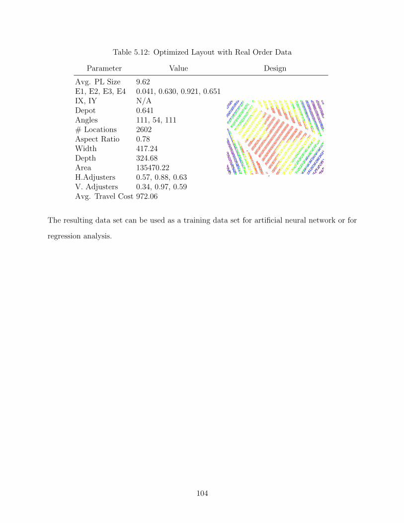
Table 5.12: Optimized Layout with Real Order Data

Parameter Value Design

Avg. PL Size 9.62E1, E2, E3, E4 0.041, 0.630, 0.921, 0.651IX, IY N/ADepot 0.641Angles 111, 54, 111# Locations 2602Aspect Ratio 0.78Width 417.24Depth 324.68Area 135470.22H.Adjusters 0.57, 0.88, 0.63V. Adjusters 0.34, 0.97, 0.59Avg. Travel Cost 972.06

The resulting data set can be used as a training data set for artificial neural network or for

regression analysis.

104

Chapter 6

Non-traditional Warehouse Design Optimization and Their Effects on Order Picking

Operations

6.1 Introduction

In this chapter, we describe our computational experiments aimed at achieving two

objectives. First, we would like to see how optimized non-traditional layouts compare to

common traditional layouts under near-optimal routing of pickers when multi-item pick lists

are present with various demand skewness from generated orders of fixed pick list size.

Second we would like to see if there are certain patterns when analyzing these results (i.e.,

how layouts are changing when pick list sizes are increasing/decreasing or demand skewness

is increasing/decreasing).

6.2 Order Generation Method

We use the model by Bender (1981) to calculate the probability of demand for each

SKU. For each SKU s, the model uses the following analytical function:

F (s) =(1 + A)s

A+ s(6.1)

where A is a shape factor that depends on the skewness of the demand. For demand

skewness pattern of 20/40 (i.e., twenty percent of most frequently picked SKUs constitute

forty percent of the picks), the value of A is 0.60. A is 0.20 and 0.07 for demand skewness

patterns of 20/60 and 20/80, respectively. The probability ps of demand for SKU s is

determined from

105

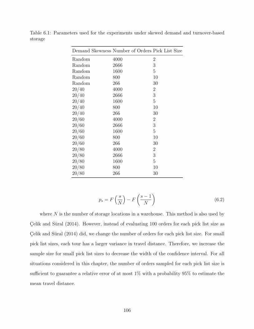
Table 6.1: Parameters used for the experiments under skewed demand and turnover-basedstorage

Demand Skewness Number of Orders Pick List Size

Random 4000 2Random 2666 3Random 1600 5Random 800 10Random 266 3020/40 4000 220/40 2666 320/40 1600 520/40 800 1020/40 266 3020/60 4000 220/60 2666 320/60 1600 520/60 800 1020/60 266 3020/80 4000 220/80 2666 320/80 1600 520/80 800 1020/80 266 30

ps = F( sN

)− F

(s− 1

N

)(6.2)

where N is the number of storage locations in a warehouse. This method is also used by

Celik and Sural (2014). However, instead of evaluating 100 orders for each pick list size as

Celik and Sural (2014) did, we change the number of orders for each pick list size. For small

pick list sizes, each tour has a larger variance in travel distance. Therefore, we increase the

sample size for small pick list sizes to decrease the width of the confidence interval. For all

situations considered in this chapter, the number of orders sampled for each pick list size is

sufficient to guarantee a relative error of at most 1% with a probability 95% to estimate the

mean travel distance.

106

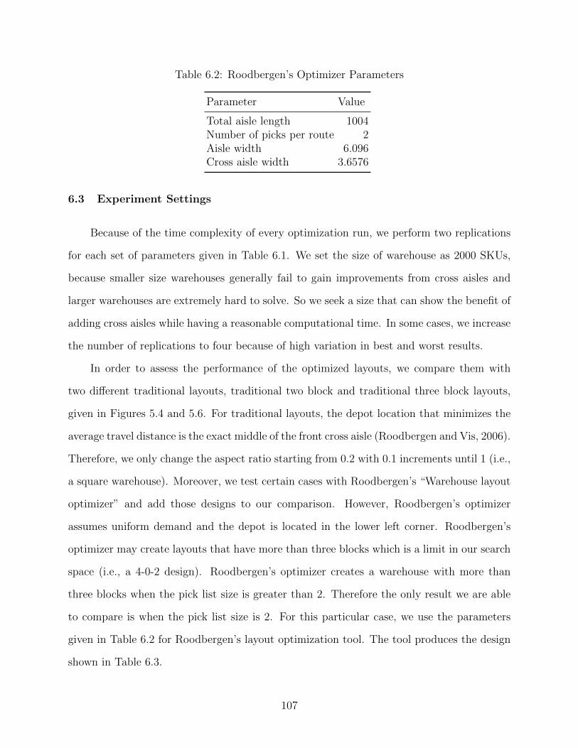
Table 6.2: Roodbergen’s Optimizer Parameters

Parameter Value

Total aisle length 1004Number of picks per route 2Aisle width 6.096Cross aisle width 3.6576

6.3 Experiment Settings

Because of the time complexity of every optimization run, we perform two replications

for each set of parameters given in Table 6.1. We set the size of warehouse as 2000 SKUs,

because smaller size warehouses generally fail to gain improvements from cross aisles and

larger warehouses are extremely hard to solve. So we seek a size that can show the benefit of

adding cross aisles while having a reasonable computational time. In some cases, we increase

the number of replications to four because of high variation in best and worst results.

In order to assess the performance of the optimized layouts, we compare them with

two different traditional layouts, traditional two block and traditional three block layouts,

given in Figures 5.4 and 5.6. For traditional layouts, the depot location that minimizes the

average travel distance is the exact middle of the front cross aisle (Roodbergen and Vis, 2006).

Therefore, we only change the aspect ratio starting from 0.2 with 0.1 increments until 1 (i.e.,

a square warehouse). Moreover, we test certain cases with Roodbergen’s “Warehouse layout

optimizer” and add those designs to our comparison. However, Roodbergen’s optimizer

assumes uniform demand and the depot is located in the lower left corner. Roodbergen’s

optimizer may create layouts that have more than three blocks which is a limit in our search

space (i.e., a 4-0-2 design). Roodbergen’s optimizer creates a warehouse with more than

three blocks when the pick list size is greater than 2. Therefore the only result we are able

to compare is when the pick list size is 2. For this particular case, we use the parameters

given in Table 6.2 for Roodbergen’s layout optimization tool. The tool produces the design

shown in Table 6.3.

107

Table 6.3: Optimal Traditional Layout with Roodbergen’s Layout Optimizer

Parameter Value Design

Skewness RandomPL Size 2E1, E2, E3, E4 0.916, 0.333, 0.833, 0.416IX, IY N/ADepot 0.72Angles 90, 90, 90# Locations 2028Aspect Ratio 1.25Width 293.09Depth 366.37Area 107379.93H.Adjusters 0.6, 0.6, 0.6V. Adjusters 0.5, 0.5, 0.5Avg. Travel Cost 712.20

Table 6.4 shows the results for generated orders and best traditional layouts selected

from a set of aspect ratio values and two different design classes (2-0-1, and 4-0-2). These

experiments are performed on four Lenovo workstations. Each workstation has a six core

hyperthreaded Intel Xeon E5-1650 processor. Workstations have 64GB of RAM and 256GB

of Solid State Drive. The operating system is 64-bit Windows 7, Enterprise Edition. The

total number of parallel threads that can be executed is 2 × 6 = 12.

6.3.1 Uniform Demand

In uniform demand, we achieve up to 3.2 percent improvement over traditional layouts.

The design we found for pick list size 3 is an interesting design with two cross aisles that meets

at the lower right corner. First cross aisle is on the middle of the back cross aisle and second

one is the 2/3rd of the left cross aisle. Both traditional three block layout and optimized

layout have similar aspect ratio and depot location (0.125 and 0.625 are symmetric). We

emphasize that this design is significantly different than previous non-traditional designs

in the literature and needs more elaboration. For other pick list sizes, the designs are not

significantly cost effective compared to their traditional counterparts. In some cases the

108

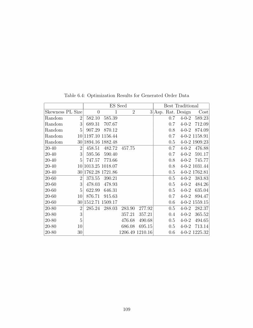
Table 6.4: Optimization Results for Generated Order Data

ES Seed Best TraditionalSkewness PL Size 0 1 2 3 Asp. Rat. Design CostRandom 2 582.10 585.39 0.7 4-0-2 589.23Random 3 689.31 707.67 0.7 4-0-2 712.09Random 5 907.29 870.12 0.8 4-0-2 874.09Random 10 1197.10 1156.44 0.7 4-0-2 1158.91Random 30 1894.16 1882.48 0.5 4-0-2 1909.2320-40 2 458.51 482.72 457.75 0.7 4-0-2 476.8820-40 3 595.56 590.40 0.7 4-0-2 591.1720-40 5 747.57 773.66 0.8 4-0-2 745.7720-40 10 1013.25 1018.07 0.8 4-0-2 1031.4420-40 30 1762.28 1721.86 0.5 4-0-2 1762.8120-60 2 373.55 390.21 0.5 4-0-2 383.8320-60 3 478.03 478.93 0.5 4-0-2 484.2620-60 5 622.99 646.31 0.5 4-0-2 635.0420-60 10 876.71 915.63 0.7 4-0-2 894.4720-60 30 1512.71 1509.17 0.6 4-0-2 1559.1520-80 2 285.24 288.03 283.90 277.92 0.5 4-0-2 282.3720-80 3 357.21 357.21 0.4 4-0-2 365.5220-80 5 476.68 490.68 0.5 4-0-2 494.6520-80 10 686.08 695.15 0.5 4-0-2 713.1420-80 30 1206.49 1210.16 0.6 4-0-2 1225.32

109

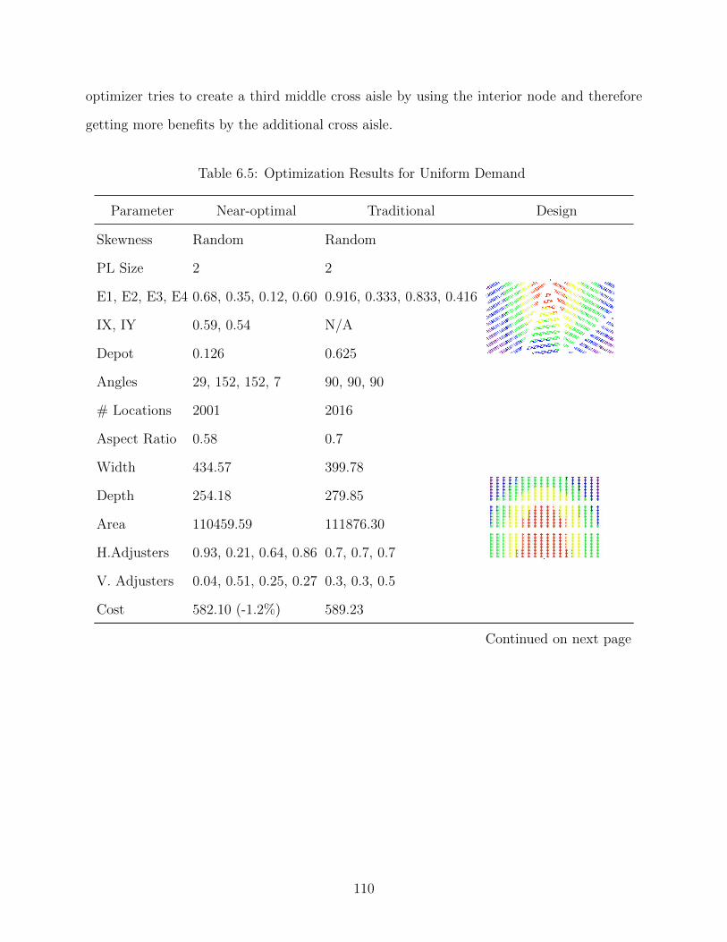
optimizer tries to create a third middle cross aisle by using the interior node and therefore

getting more benefits by the additional cross aisle.

Table 6.5: Optimization Results for Uniform Demand

Parameter Near-optimal Traditional Design

Skewness Random Random

PL Size 2 2

E1, E2, E3, E4 0.68, 0.35, 0.12, 0.60 0.916, 0.333, 0.833, 0.416

IX, IY 0.59, 0.54 N/A

Depot 0.126 0.625

Angles 29, 152, 152, 7 90, 90, 90

# Locations 2001 2016

Aspect Ratio 0.58 0.7

Width 434.57 399.78

Depth 254.18 279.85

Area 110459.59 111876.30

H.Adjusters 0.93, 0.21, 0.64, 0.86 0.7, 0.7, 0.7

V. Adjusters 0.04, 0.51, 0.25, 0.27 0.3, 0.3, 0.5

Cost 582.10 (-1.2%) 589.23

Continued on next page

110

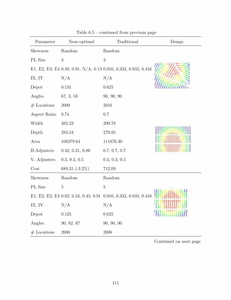
Table 6.5 – continued from previous page

Parameter Near-optimal Traditional Design

Skewness Random Random

PL Size 3 3

E1, E2, E3, E4 0.49, 0.91, N/A, 0.13 0.916, 0.333, 0.833, 0.416

IX, IY N/A N/A

Depot 0.131 0.625

Angles 67, 3, 58 90, 90, 90

# Locations 2000 2016

Aspect Ratio 0.74 0.7

Width 382.23 399.78

Depth 283.54 279.85

Area 108379.64 111876.30

H.Adjusters 0.42, 0.21, 0.86 0.7, 0.7, 0.7

V. Adjusters 0.3, 0.3, 0.5 0.3, 0.3, 0.5

Cost 689.31 (-3.2%) 712.09

Skewness Random Random

PL Size 5 5

E1, E2, E3, E4 0.82, 0.34, 0.43, 0.91 0.916, 0.333, 0.833, 0.416

IX, IY N/A N/A

Depot 0.125 0.625

Angles 90, 82, 87 90, 90, 90

# Locations 2000 2006

Continued on next page

111

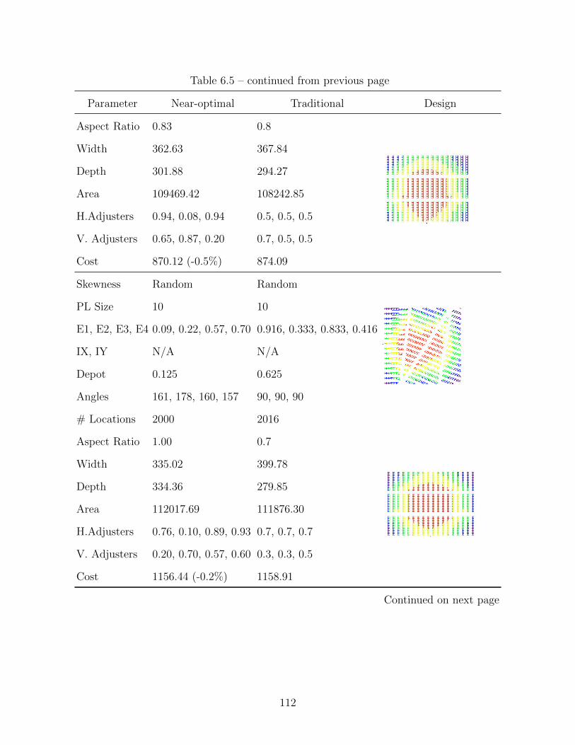
Table 6.5 – continued from previous page

Parameter Near-optimal Traditional Design

Aspect Ratio 0.83 0.8

Width 362.63 367.84

Depth 301.88 294.27

Area 109469.42 108242.85

H.Adjusters 0.94, 0.08, 0.94 0.5, 0.5, 0.5

V. Adjusters 0.65, 0.87, 0.20 0.7, 0.5, 0.5

Cost 870.12 (-0.5%) 874.09

Skewness Random Random

PL Size 10 10

E1, E2, E3, E4 0.09, 0.22, 0.57, 0.70 0.916, 0.333, 0.833, 0.416

IX, IY N/A N/A

Depot 0.125 0.625

Angles 161, 178, 160, 157 90, 90, 90

# Locations 2000 2016

Aspect Ratio 1.00 0.7

Width 335.02 399.78

Depth 334.36 279.85

Area 112017.69 111876.30

H.Adjusters 0.76, 0.10, 0.89, 0.93 0.7, 0.7, 0.7

V. Adjusters 0.20, 0.70, 0.57, 0.60 0.3, 0.3, 0.5

Cost 1156.44 (-0.2%) 1158.91

Continued on next page

112

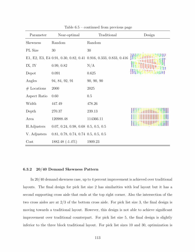
Table 6.5 – continued from previous page

Parameter Near-optimal Traditional Design

Skewness Random Random

PL Size 30 30

E1, E2, E3, E4 0.91, 0.30, 0.82, 0.41 0.916, 0.333, 0.833, 0.416

IX, IY 0.99, 0.82 N/A

Depot 0.091 0.625

Angles 94, 84, 92, 91 90, 90, 90

# Locations 2000 2025

Aspect Ratio 0.60 0.5

Width 447.49 478.26

Depth 270.37 239.13

Area 120988.48 114366.11

H.Adjusters 0.07, 0.24, 0.98, 0.68 0.5, 0.5, 0.5

V. Adjusters 0.81, 0.78, 0.74, 0.74 0.5, 0.5, 0.5

Cost 1882.48 (-1.4%) 1909.23

6.3.2 20/40 Demand Skewness Pattern

In 20/40 demand skewness case, up to 4 percent improvement is achieved over traditional

layouts. The final design for pick list size 2 has similarities with leaf layout but it has a

second supporting cross aisle that ends at the top right corner. Also the intersection of the

two cross aisles are at 2/3 of the bottom cross aisle. For pick list size 3, the final design is

moving towards a traditional layout. However, this design is not able to achieve significant

improvement over traditional counterpart. For pick list size 5, the final design is slightly

inferior to the three block traditional layout. For pick list sizes 10 and 30, optimization is

113

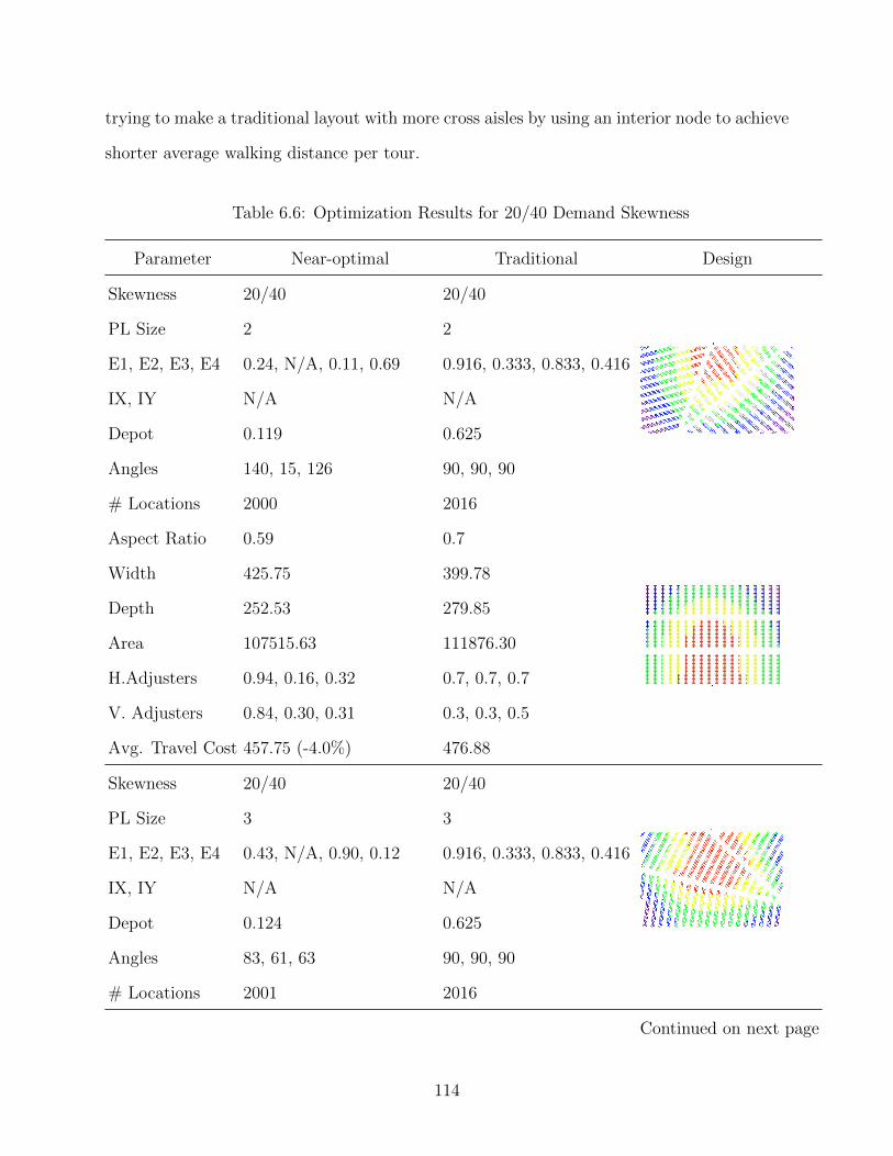
trying to make a traditional layout with more cross aisles by using an interior node to achieve

shorter average walking distance per tour.

Table 6.6: Optimization Results for 20/40 Demand Skewness

Parameter Near-optimal Traditional Design

Skewness 20/40 20/40

PL Size 2 2

E1, E2, E3, E4 0.24, N/A, 0.11, 0.69 0.916, 0.333, 0.833, 0.416

IX, IY N/A N/A

Depot 0.119 0.625

Angles 140, 15, 126 90, 90, 90

# Locations 2000 2016

Aspect Ratio 0.59 0.7

Width 425.75 399.78

Depth 252.53 279.85

Area 107515.63 111876.30

H.Adjusters 0.94, 0.16, 0.32 0.7, 0.7, 0.7

V. Adjusters 0.84, 0.30, 0.31 0.3, 0.3, 0.5

Avg. Travel Cost 457.75 (-4.0%) 476.88

Skewness 20/40 20/40

PL Size 3 3

E1, E2, E3, E4 0.43, N/A, 0.90, 0.12 0.916, 0.333, 0.833, 0.416

IX, IY N/A N/A

Depot 0.124 0.625

Angles 83, 61, 63 90, 90, 90

# Locations 2001 2016

Continued on next page

114

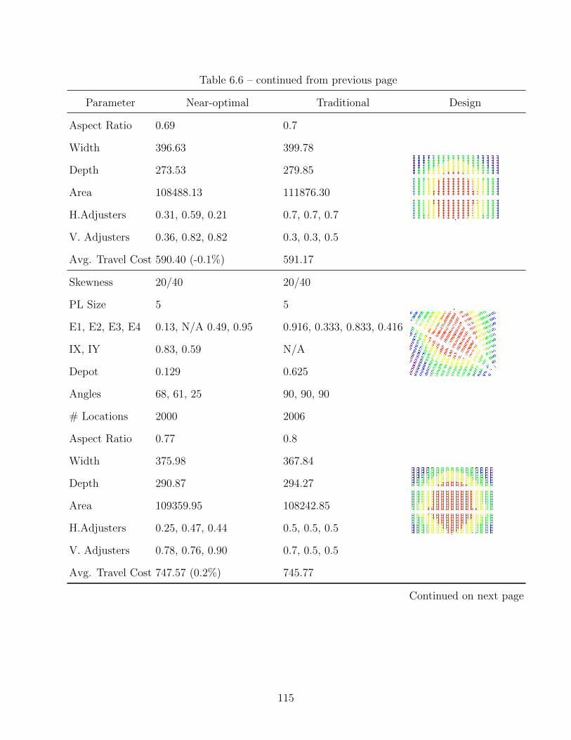
Table 6.6 – continued from previous page

Parameter Near-optimal Traditional Design

Aspect Ratio 0.69 0.7

Width 396.63 399.78

Depth 273.53 279.85

Area 108488.13 111876.30

H.Adjusters 0.31, 0.59, 0.21 0.7, 0.7, 0.7

V. Adjusters 0.36, 0.82, 0.82 0.3, 0.3, 0.5

Avg. Travel Cost 590.40 (-0.1%) 591.17

Skewness 20/40 20/40

PL Size 5 5

E1, E2, E3, E4 0.13, N/A 0.49, 0.95 0.916, 0.333, 0.833, 0.416

IX, IY 0.83, 0.59 N/A

Depot 0.129 0.625

Angles 68, 61, 25 90, 90, 90

# Locations 2000 2006

Aspect Ratio 0.77 0.8

Width 375.98 367.84

Depth 290.87 294.27

Area 109359.95 108242.85

H.Adjusters 0.25, 0.47, 0.44 0.5, 0.5, 0.5

V. Adjusters 0.78, 0.76, 0.90 0.7, 0.5, 0.5

Avg. Travel Cost 747.57 (0.2%) 745.77

Continued on next page

115

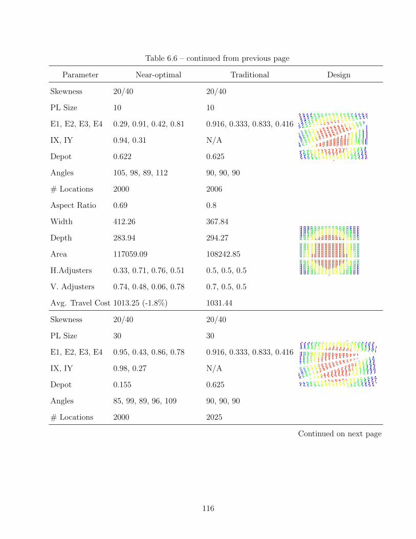
Table 6.6 – continued from previous page

Parameter Near-optimal Traditional Design

Skewness 20/40 20/40

PL Size 10 10

E1, E2, E3, E4 0.29, 0.91, 0.42, 0.81 0.916, 0.333, 0.833, 0.416

IX, IY 0.94, 0.31 N/A

Depot 0.622 0.625

Angles 105, 98, 89, 112 90, 90, 90

# Locations 2000 2006

Aspect Ratio 0.69 0.8

Width 412.26 367.84

Depth 283.94 294.27

Area 117059.09 108242.85

H.Adjusters 0.33, 0.71, 0.76, 0.51 0.5, 0.5, 0.5

V. Adjusters 0.74, 0.48, 0.06, 0.78 0.7, 0.5, 0.5

Avg. Travel Cost 1013.25 (-1.8%) 1031.44

Skewness 20/40 20/40

PL Size 30 30

E1, E2, E3, E4 0.95, 0.43, 0.86, 0.78 0.916, 0.333, 0.833, 0.416

IX, IY 0.98, 0.27 N/A

Depot 0.155 0.625

Angles 85, 99, 89, 96, 109 90, 90, 90

# Locations 2000 2025

Continued on next page

116

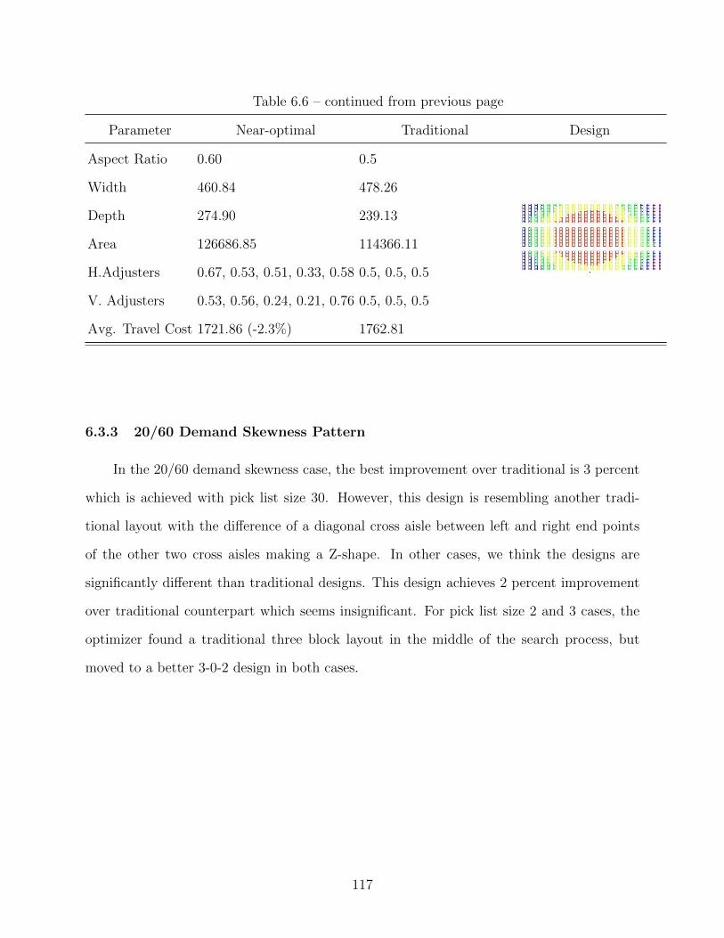
Table 6.6 – continued from previous page

Parameter Near-optimal Traditional Design

Aspect Ratio 0.60 0.5

Width 460.84 478.26

Depth 274.90 239.13

Area 126686.85 114366.11

H.Adjusters 0.67, 0.53, 0.51, 0.33, 0.58 0.5, 0.5, 0.5

V. Adjusters 0.53, 0.56, 0.24, 0.21, 0.76 0.5, 0.5, 0.5

Avg. Travel Cost 1721.86 (-2.3%) 1762.81

6.3.3 20/60 Demand Skewness Pattern

In the 20/60 demand skewness case, the best improvement over traditional is 3 percent

which is achieved with pick list size 30. However, this design is resembling another tradi-

tional layout with the difference of a diagonal cross aisle between left and right end points

of the other two cross aisles making a Z-shape. In other cases, we think the designs are

significantly different than traditional designs. This design achieves 2 percent improvement

over traditional counterpart which seems insignificant. For pick list size 2 and 3 cases, the

optimizer found a traditional three block layout in the middle of the search process, but

moved to a better 3-0-2 design in both cases.

117

Table 6.7: Optimization Results for 20/60 Demand Skewness

Parameter Near-optimal Traditional Design

Skewness 20/60 20/60

PL Size 2 2

E1, E2, E3, E4 0.03, 0.13, 0.58, 0.59 0.916, 0.333, 0.833, 0.416

IX, IY N/A N/A

Depot 0.123 0.625

Angles 156, 41, 51 90, 90, 90

# Locations 2000 2025

Aspect Ratio 0.54 0.5

Width 447.39 478.26

Depth 239.84 239.13

Area 107300.71 114366.11

H.Adjusters 0.78, 0.41, 0.56 0.5, 0.5, 0.5

V. Adjusters 0.22, 0.26, 0.48 0.5, 0.5, 0.5

Avg. Travel Cost 373.55 (-2.7%) 383.83

Skewness 20/60

PL Size 3 3

E1, E2, E3, E4 0.83, N/A, N/A, 0.98 0.916, 0.333, 0.833, 0.416

IX, IY 0.98, 0.51 N/A

Depot 0.121 0.625

Angles 94, 75 90, 90, 90

# Locations 2000 2025

Continued on next page

118

Table 6.7 – continued from previous page

Parameter Near-optimal Traditional Design

Aspect Ratio 0.62 0.5

Width 423.70 478.26

Depth 260.96 239.13

Area 110570.16 114366.11

H.Adjusters 0.18, 0.34 0.5, 0.5, 0.5

V. Adjusters 0.45, 0.07 0.5, 0.5, 0.5

Avg. Travel Cost 478.03 (-1.2%) 484.26

Skewness 20/60 20/60

PL Size 5 5

E1, E2, E3, E4 0.78, N/A, 0.30, 0.92 0.916, 0.333, 0.833, 0.416

IX, IY N/A N/A

Depot 0.125 0.625

Angles 91, 113, 95 90, 90, 90

# Locations 2000 2025

Aspect Ratio 0.62 0.5

Width 421.44 478.26

Depth 262.36 239.13

Area 110570.16 114366.11

H.Adjusters 0.87, 0.35, 0.17 0.5, 0.5, 0.5

V. Adjusters 0.40, 0.17, 0.20 0.5, 0.5, 0.5

Avg. Travel Cost 622.99 (-1.8%) 635.04

Continued on next page

119

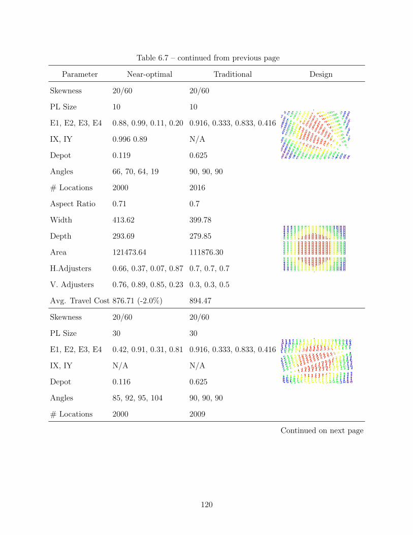
Table 6.7 – continued from previous page

Parameter Near-optimal Traditional Design

Skewness 20/60 20/60

PL Size 10 10

E1, E2, E3, E4 0.88, 0.99, 0.11, 0.20 0.916, 0.333, 0.833, 0.416

IX, IY 0.996 0.89 N/A

Depot 0.119 0.625

Angles 66, 70, 64, 19 90, 90, 90

# Locations 2000 2016

Aspect Ratio 0.71 0.7

Width 413.62 399.78

Depth 293.69 279.85

Area 121473.64 111876.30

H.Adjusters 0.66, 0.37, 0.07, 0.87 0.7, 0.7, 0.7

V. Adjusters 0.76, 0.89, 0.85, 0.23 0.3, 0.3, 0.5

Avg. Travel Cost 876.71 (-2.0%) 894.47

Skewness 20/60 20/60

PL Size 30 30

E1, E2, E3, E4 0.42, 0.91, 0.31, 0.81 0.916, 0.333, 0.833, 0.416

IX, IY N/A N/A

Depot 0.116 0.625

Angles 85, 92, 95, 104 90, 90, 90

# Locations 2000 2009

Continued on next page

120

Table 6.7 – continued from previous page

Parameter Near-optimal Traditional Design

Aspect Ratio 0.63 0.6

Width 432.11 430.30

Depth 270.90 258.18

Area 117059.08 111095.51

H.Adjusters 0.37, 0.70, 0.83, 0.96 0.1, 0.1, 0.1

V. Adjusters 0.90, 0.32, 0.75, 0.77 0.9, 0.9, 0.5

Avg. Travel Cost 1512.72 (-3.0%) 1559.15

6.3.4 20/80 Demand Skewness Pattern

In the 20/80 demand skewness case, maximum improvement over traditional is 3.8

percent in pick list size 10. We can definitely see a pattern in the designs which create a

diagonal aisle between 1/2 or 2/3 of the left or right cross aisles. The region closest to the

depot location becomes 90 degrees with the region next to it is about 15-20 degrees rotated

to one of the sides (75, 101, or 111 degrees). Farthest regions to the depot location are more

similar to traditional one block layout.

121

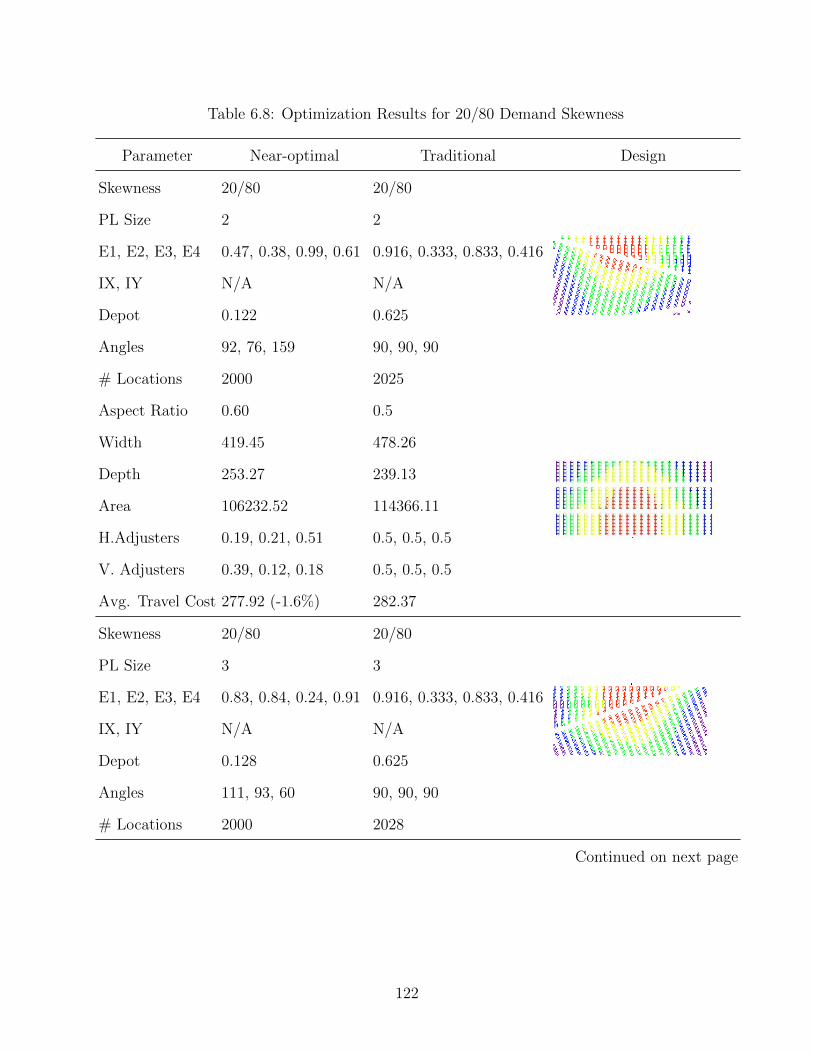
Table 6.8: Optimization Results for 20/80 Demand Skewness

Parameter Near-optimal Traditional Design

Skewness 20/80 20/80

PL Size 2 2

E1, E2, E3, E4 0.47, 0.38, 0.99, 0.61 0.916, 0.333, 0.833, 0.416

IX, IY N/A N/A

Depot 0.122 0.625

Angles 92, 76, 159 90, 90, 90

# Locations 2000 2025

Aspect Ratio 0.60 0.5

Width 419.45 478.26

Depth 253.27 239.13

Area 106232.52 114366.11

H.Adjusters 0.19, 0.21, 0.51 0.5, 0.5, 0.5

V. Adjusters 0.39, 0.12, 0.18 0.5, 0.5, 0.5

Avg. Travel Cost 277.92 (-1.6%) 282.37

Skewness 20/80 20/80

PL Size 3 3

E1, E2, E3, E4 0.83, 0.84, 0.24, 0.91 0.916, 0.333, 0.833, 0.416

IX, IY N/A N/A

Depot 0.128 0.625

Angles 111, 93, 60 90, 90, 90

# Locations 2000 2028

Continued on next page

122

Table 6.8 – continued from previous page

Parameter Near-optimal Traditional Design

Aspect Ratio 0.48 0.4

Width 465.81 542.52

Depth 223.32 217.01

Area 104023.80 117733.00

H.Adjusters 0.52, 0.28, 0.80 0.5, 0.5, 0.5

V. Adjusters 0.21, 0.17, 0.23 0.5, 0.5, 0.5

Avg. Travel Cost 357.21 (-2.2%) 365.52

Skewness 20/80 20/80

PL Size 5 5

E1, E2, E3, E4 0.37, N/A, 0.67, 0.21 0.916, 0.333, 0.833, 0.416

IX, IY 0.04, 0.46 N/A

Depot 0.120 0.625

Angles 91, 111, 91 90, 90, 90

# Locations 2000 2025

Aspect Ratio 0.54 0.5

Width 464.20 478.26

Depth 249.17 239.13

Area 115662.07 114366.11

H.Adjusters 0.69, 0.82, 0.78 0.5, 0.5, 0.5

V. Adjusters 0.33, 0.62, 0.09 0.5, 0.5, 0.5

Avg. Travel Cost 476.68 (-3.6%) 494.65

Continued on next page

123

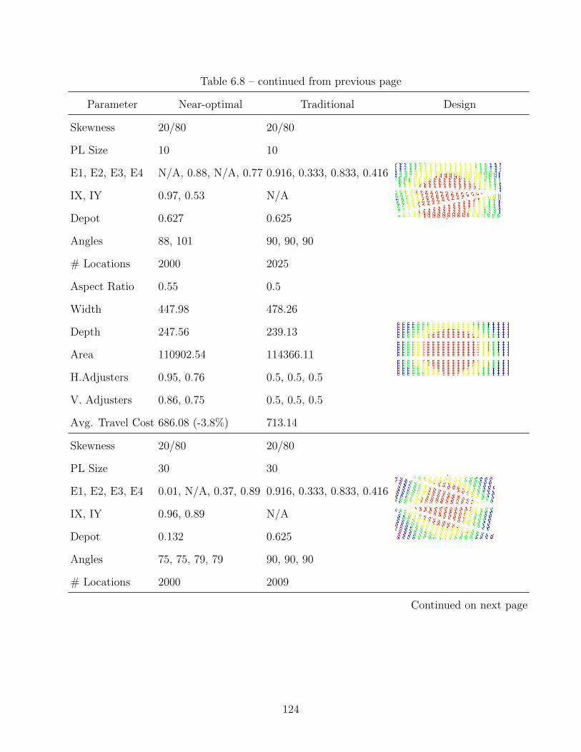
Table 6.8 – continued from previous page

Parameter Near-optimal Traditional Design

Skewness 20/80 20/80

PL Size 10 10

E1, E2, E3, E4 N/A, 0.88, N/A, 0.77 0.916, 0.333, 0.833, 0.416

IX, IY 0.97, 0.53 N/A

Depot 0.627 0.625

Angles 88, 101 90, 90, 90

# Locations 2000 2025

Aspect Ratio 0.55 0.5

Width 447.98 478.26

Depth 247.56 239.13

Area 110902.54 114366.11

H.Adjusters 0.95, 0.76 0.5, 0.5, 0.5

V. Adjusters 0.86, 0.75 0.5, 0.5, 0.5

Avg. Travel Cost 686.08 (-3.8%) 713.14

Skewness 20/80 20/80

PL Size 30 30

E1, E2, E3, E4 0.01, N/A, 0.37, 0.89 0.916, 0.333, 0.833, 0.416

IX, IY 0.96, 0.89 N/A

Depot 0.132 0.625

Angles 75, 75, 79, 79 90, 90, 90

# Locations 2000 2009

Continued on next page

124

Table 6.8 – continued from previous page

Parameter Near-optimal Traditional Design

Aspect Ratio 0.65 0.6

Width 422.47 430.30

Depth 275.70 258.18

Area 116474.96 111095.51

H.Adjusters 0.14, 0.18, 0.60, 0.93 0.1, 0.1, 0.1

V. Adjusters 0.06, 0.16, 0.86, 0.82 0.9, 0.9, 0.5

Avg. Travel Cost 1206.49 (-1.5%) 1225.32

6.4 Summary

This research has shown that some non-traditional layouts are robust for several pick

list sizes and demand skewnesses. To the author’s knowledge, this is the first reported

application of layout optimization for order picking operations, comparisons of parallel and

distributed large batches of TSP solvers, and realistic path finding in warehouses.

In Chapter 3, parallel and distributed computing of well known heuristic and exact TSP

solvers (LKH and Concorde) are proposed. They provide higher CPU utilization compared

to other published parallel TSP solvers. Various applications of large batches of TSPs and a

detailed graphic representation of methodology are given. We compared serial, parallel, and

distributed solver implementations. These implementations are found to be easy to program

and highly efficient compared to serial implementations. Our results indicate that parallel

computing using hyper-threading for solving 150- and 200-city TSPs can increase the overall

utilization of computer resources up to 25 percent compared to single thread computing.

The resulting speed-up/physical core ratios are as much as ten times better than the parallel

and concurrent version of the LKH heuristic using SPC3 in the literature. For variable TSP

125

sizes, a longest processing time first heuristic performs better than an equal distribution rule.

We illustrated our approach with an application in the design of order picking warehouses.

In Chapter 4, we introduce the visibility graph as a new way of estimating the length

of a route traveled by order pickers in a warehouse. Following aisle centers leads to longer

travel distances when an order picker picks items within picking aisles which have angles

other than 90 degrees between cross aisles. Details of the visibility graph implementation

are given in the context of warehouse design. We present and compare results for tradi-

tional and fishbone layouts. Our results show that the visibility graph method changes the

assessment of the fishbone layout as high as 9% compared to the traditional counterpart.

Moreover, we analyze the affect of the visibility graph method for selecting the best lay-

out that minimizes the average travel cost from three most common traditional layouts.

By using the visibility graph method, we find a different layout in 13% of the cases than

the previous distance estimation method used in the literature. We anticipate that visibility

graph method can be readily integrated into warehouse layout optimization and comparison.

Furthermore, distance estimation is an important aspect of retail layout design and other

applications in facility layout design, and the visibility graph method will be also relevant

for such applications.

In Chapter 5, we present a computational system to solve the warehouse aisle design

problem. This system allows cross aisles and pick aisles to take on any angle. It produces

near-optimal designs for nineteen design classes including design classes with an interior

point.

In Chapter 6, we show that these new non-traditional designs can decrease average

travel distance up to 4% compared to traditional counterparts. For small pick list sizes,

because of the greater importance of the depot location to travel cost, layouts are designed

with vertical cross aisles. As the pick list size increases, these cross aisles become horizontal

allowing better access between storage locations. We anticipate our approach to be a starting

point for more detailed research for warehouse layout optimization.

126

During our experiments we evaluated over 4.8 billion TSPs. These calculations took over

two months period on four workstations. We believe this can be improved by eliminating

LKH and implementing our own TSP solver inside our system. Also, graphical processing

units (GPUs) can be used in complex calculations and the design search space can be enlarged

by adding more external and internal nodes to potentially find better designs for order picking

operations. We can investigate other routing and storage policies and embed these into the

encoding scheme as variables so that we can choose a layout, a routing and a storage policy

for a given environment.

For future research, we will implement a more efficient shortest path mapping method

and compare computational times between two methods for different size warehouses. More-

over, we will develop paths and travel time models that consider not only linear paths but

also non-linear paths around the corners of pick aisles.

127

Bibliography

Ackerman, K. B., Gardner, R. W., and Thomas, L. P. (1972). Understanding today’s distri-

bution center. Traffic Service Corp.

Angeniol, B., Vaubois, G. D. L. C., and Le Texier, J.-Y. (1988). Self-organizing feature maps

and the travelling salesman problem. Neural Networks, 1(4):289–293.

Applegate, D. L., Bixby, R. E., Chvatal, V., and Cook, W. J. (2007). The Traveling Salesman

Problem: A Computational Study. Princeton University Press.

Aziz, I. A., Haron, N., Mehat, M., Jung, L., Mustapa, A. N., and Akhir, E. (2009). Solving

traveling salesman problem on cluster compute nodes. WSEAS Transactions on Comput-

ers, (6):1020–1029.

Back, T. and Schutz, M. (1995). Evolution strategies for mixed-integer optimization of

optical multilayer systems. In Evolutionary Programming IV: Proceedings of the Fourth

Annual Conference on Evolutionary Programming, pages 33–51.

Baltar, A. M. and Fontane, D. G. (2006). A generalized multiobjective particle swarm opti-

mization solver for spreadsheet models: application to water quality. In AGU Hydrology

Days 2006, pages 1–12.

Bartholdi, J. J. and Hackman, S. T. (2011). Warehouse & Distribution Science. Georgia

Institute of Technology.

Bassan, Y., Roll, Y., and Rosenblatt, M. J. (1980). Internal layout design of a warehouse.

A I I E Transactions, 12(4):317–322.

Bellman, R. (1958). On a routing problem. Quarterly of Applied Mathematics, 16:87–90.

128

Bender, P. S. (1981). Mathematical modeling of the 20/80 rule: theory and practice. Journal

of Business Logistics, 2(2):139–157.

Berglund, P. and Batta, R. (2012). Optimal placement of warehouse cross-aisles in a picker-

to-part warehouse with class-based storage. IIE Transactions, 44(2):107–120.

Beyer, H.-G. (1992). Some aspects of the evolution strategy for solving TSP-like optimization

problems appearing at the design studies of a 0.5tev e +e- -linear collider. In Parallel

Problem Solving from Nature, volume 2, pages 361–370. Elsevier.

Bond, J. (2015). Top 20 3pl and public refrigerated warehouses, 2015. http://www.mmh.com/

article/top_20_3pl_and_public_refrigerated_warehouses_2015. Online Accessed

04.25.2017.

Canny, J. and Reif, J. (1987). New lower bound techniques for robot motion planning

problems. In Foundations of Computer Science, 1987., 28th Annual Symposium on, pages

49–60. IEEE.

Casey, S. (2011 [accessed 06.13.2016]). How to determine the effectiveness of hyper-

threading technology with an application. https://software.intel.com/en-us/articles/how-

to-determine-the-effectiveness-of-hyper-threading-technology-with-an-application/.

Cedeno, W. and Agrafiotis, D. K. (2003). Using particle swarm for the development of qsar

models based on k-nearest neighbor and kernel regression. Journal of Computer-Aided,

17:255–263.

Celik, M. and Sural, H. (2014). Order picking under random and turnover-based storage

policies in fishbone aisle warehouses. IIE Transactions, 46(3):283–300.

Cesari, G. (1996). Divide and conquer strategies for parallel TSP heuristics. Computers &

Operations Research, 23(7):681–694.

129

Chen, F., Wang, H., Qi, C., and Xie, Y. (2013). An ant colony optimization routing algorithm

for two order pickers with congestion consideration. Computers & Industrial Engineering,

66(1):77–85.

Choe, K. and Sharp, G. (1991). Small parts order picking: Design and op-

eration. http://www2.isye.gatech.edu/~mgoetsch/cali/Logistics%20Tutorial/

order/article.htm. Online Accessed 06.22.2013.

Cook, W. (2014). In pursuit of the traveling salesman: mathematics at the limits of compu-

tation. Princeton University Press.

Cordon, O., Herrera, F., and Sanchez, L. (1998). Evolutionary Learning Processes for Data

Analysis in Electrical Engineering Applications. John Wiley and Sons.

Cutello, V., Narzisi, G., and Nicosia, G. (2005). A class of Pareto archived evolution strategy

algorithms using immune inspired operators for ab-initio protein structure prediction. In

Applications on Evolutionary Computing, Proceedings of EvoWorkkshops 2005, pages 54–

63.

Dallari, F., Marchet, G., and Melacini, M. (2009). Design of order picking system. The

International Journal of Advanced Manufacturing Technology, 42(1-2):1–12.

Daniels, R. L., Rummel, J. L., and Schantz, R. (1998). A model for warehouse order picking.

European Journal of Operational Research, 105:1–17.

De Koster, R., Le-Duc, T., and Roodbergen, K. J. (2007). Design and control of warehouse

order picking: A literature review. European Journal of Operational Research, 182:481 –

501.

De Koster, R. and Poort, E. (1998). Routing order-pickers in a warehouse: a comparison

between optimal and heuristic solutions. IIE Transactions, 30(5):469–480.

130

Dijkstra, E. W. (1959). A note on two problems in connexion. Numerische Mathematik,

1:269–271.

Dorigo, M. and Gambardella, L. M. (1997). Ant colonies for the travelling salesman problem.

BioSystems, 43(2):73–81.

Dukic, G. and Opetuk, T. (2008). Analysis of order-picking in warehouses with fishbone

layout. In Proceedings of the 2008 International Conference on Industrial Logistics, pages

197–205.

Emmerich, M., Grtzner, M., Gro, B., and Schtz, M. (2000). Mixed-integer evolution strategy

for chemical plant optimization with simulators. http://www.liacs.nl/~emmerich/pdf/

EGG+00.pdf. Online Accessed 02.09.2014.

Floyd, R. W. (1962). Algorithm 97: shortest path. Communications of the ACM, 5(6):345.

Ford, L. R. (1956). Network Flow Theory. Rand Corporation.

Francis, R. L. (1967). On some problems of rectangular warehouse design and layout. Journal

of Industrial Engineering, 18(10):595–604.

Frazelle, E., Hackman, S., Passy, U., and Platzman, L. (1994). Optimization in industry 2.

In Ciriani., A. T. and Leachman, R. C., editors, Optimization in Industry 2, chapter The

Forward-reserve Problem, pages 43–61. John Wiley & Sons, Inc., New York, NY, USA.

Frazelle, E. H. (2002). World-Class Warehousing and Material Handling, volume 1. McGraw-

Hill New York.

Gallo, G. and Pallottino, S. (1986). Shortest path methods: a unifying approach. In Netflow

at Pisa, pages 38–64. Springer.

Garey, M. R. and Johnson, D. S. (1979). Computers and intractability: a guide to NP-

completeness. WH Freeman New York.

131

Gensler, L. (2016). The world’s largest retailers 2016: Wal-mart dominates but ama-

zon is catching up. https://www.forbes.com/sites/laurengensler/2016/05/27/

global-2000-worlds-largest-retailers/. Online Accessed 04.16.2017.

Ghosh, S. K. and Mount, D. M. (1991). An output-sensitive algorithm for computing visi-

bility graphs. SIAM Journal on Computing, 20(5):888–910.

Goetschalckx, M. and Ashayeri, J. (1989). Classification and design of order picking. Logistics

Information Management, 2:99–106.

Goetschalckx, M. and Ratliff, H. D. (1988). Order picking in an aisle. IIE Transactions,

20:53–62.

Graham, R. L. (1969). Bounds on multiprocessing timing anomalies. SIAM Journal on

Applied Mathematics, 17(2):416–429.

Grefenstette, J., Gopal, R., Rosmaita, B., and Van Gucht, D. (1985). Genetic algorithms

for the traveling salesman problem. In Proceedings of the First International Conference

on Genetic Algorithms and their Applications, pages 160–168. Lawrence Erlbaum, New

Jersey (160-168).

Greiner, H. (1996). Robust optical coating design with evolutionary strategies. Applied

Optics, 35(28):5477–5483.

Gu, J. (2005). The Forward Reserve Warehouse Sizing and Dimensioning Problem. PhD

thesis, Georgia Institute of Technology.

Gu, J., Goetschalckx, M., and McGinnis, L. F. (2007). Research on warehouse operation: A

comprehensive review. European Journal of Operational Research, 177:1–21.

Gue, K. R. and Meller, R. D. (2009). Aisle configurations for unit-load warehouses. IIE

Transactions on Design & Manufacturing, 41(3):171–182.

132

Hackman, S. T., Rosenblatt, M. J., and Olin, J. M. (1990). Allocating items to an automated

storage and retrieval system. IIE Transactions, 22(1):7–14.

Hall, R. W. (1993). Distance approximation for routing manual pickers in a warehouse. IIE

Transactions, 25(4):76–87.

Hart, P. E., Nilsson, N. J., and Raphael, B. (1968). A formal basis for the heuristic determi-

nation of minimum cost paths. Systems Science and Cybernetics, IEEE Transactions on,

4(2):100–107.

Held, M. and Karp, R. M. (1962). A dynamic programming approach to sequencing problems.

Journal of the Society for Industrial and Applied Mathematics, pages 196–210.

Helsgaun, K. (2000). An effective implementation of the lin-kernighan traveling salesman

heuristic. European Journal of Operational Research, 126:106–130.

Hershberger, J. and Suri, S. (1999). An optimal algorithm for euclidean shortest paths in

the plane. SIAM Journal on Computing, 28(6):2215–2256.

Heskett, J. L. (1963). Cube-per-order index - a key to warehouse stock location. Transport

and Distribution Management, 3:27–31.

Heskett, J. L. (1964). Putting the cube-per-order index to work in warehouse layout. Trans-

port and Distribution Management, 4:23–30.

Hsieh, L.-f. and Tsai, L. (2006). The optimum design of a warehouse system on order picking

efficiency. The International Journal of Advanced Manufacturing Technology, 28(5-6):626–

637.

Huang, H., Yang, J. T., Shen, S. F., and Horng, J.-T. (1999). An evolution strategy to solve

sports scheduling problems. In Proceedings of the Genetic and Evolutionary Computation

Conference GECCO-99, volume 1, page 943.

133

Ismail, M. A., Mirza, S. H., and Altaf, T. (2011). A parallel and concurrent implementation

of lin-kernighan heuristic (lkh-2) for solving traveling salesman problem for multi-core

processors using SPC3 programming model. IJACSA Editorial.

Johnson, D. B. (1977). Efficient algorithms for shortest paths in sparse networks. Journal

of the ACM (JACM), 24(1):1–13.

Keller, R. E., Banzhaf, W., Mehnen, J., and Weinert, K. (1999). CAD surface reconstruction

from digitized 3D point data with a genetic programming/evolution strategy hybrid. In

Advances in Genetic Programming, volume 3, chapter 3, pages 41–65. The MIT Press.

Kennedy, J. and Eberhart, R. (1995). Particle swarm optimization. In Neural Networks,

1995. Proceedings., IEEE International Conference on, volume 4, pages 1942–1948.

Kirkpatrick, S. (1984). Optimization by simulated annealing: Quantitative studies. Journal

of Statistical Physics, 34(5-6):975–986.

Knox, J. (1994). Tabu search performance on the symmetric traveling salesman problem.

Computers & Operations Research, 21(8):867–876.

Kraay, D. R. and Harker, P. T. (1997). Case-based reasoning for repetitive combinatorial

optimization problems, part II: numerical results. Journal of Heuristics, 3(1):25–42.

Kubota, S., Onoyama, T., Oyanagi, K., and Tsuruta, S. (1999). Traveling salesman problem

solving method fit for interactive repetitive simulation of large-scale distribution networks.

In Systems, Man, and Cybernetics, 1999. IEEE SMC’99 Conference Proceedings. 1999

IEEE International Conference on, volume 3, pages 533–538. IEEE.

Kunder, R. and Gudehus, T. (1975). Mittlere wegzeiten beim eindimensionalen kommission-

ieren. Zeitschrift fr Operations Research, 19(2):B53–B72.

134

Lazarova, M. and Borovska, P. (2008). Comparison of parallel metaheuristics for solving

the tsp. In Proceedings of the 9th International Conference on Computer Systems and

Technologies and Workshop for PhD Students in Computing, page 17. ACM.

Le-Duc, T. (2005). Design and Control of Efficient Order Picking Process. PhD thesis,

Erasmus University Rotterdam.

Li, R., Emmerich, M. T. M., Eggermont, J., and Bovenkamp, E. G. P. (2006). Mixed-integer

optimization of coronary vessel image analysis using evolution strategies. In GECCO06:

Proceedings of the 8th Annual Conference on Genetic and Evolutionary Computation,

pages 1645–1652.

Lin, S. and Kernighan, B. W. (1973). An effective heuristic algorithm for the traveling

salesman problem. Operations Research, 21:498–516.

Lourenco, H. R., Martin, O. C., and Stutzle, T. (2003). Handbook of Metaheuristics, chapter

Iterated Local Search, pages 320–353. Springer US, Boston, MA.

Makris, P. A. and Giakoumakis, I. G. (2003). k-interchange heuristic as an optimization

procedure for material handling applications. Applied Mathematical Modelling, 27:345–

358.

Malmborg, C. J. and Bhaskaran, K. (1987). On the optimality of the cube per order index

for conventional warehouses with dual command cycles. Material Flow, 4:169–175.

Meissner, M., Schmuker, M., and Schneider, G. (2006). Optimized particle swarm optimiza-

tion (opso) and its application to artificial neural network training. BMC Bioinformatics,

7(125).

Meller, R. D. and Gue, K. R. (2009). The application of new aisle designs for unit-load

warehouses. In NSF Engineering Research and Innovation Conference.

Moore, E. F. (1959). The shortest path through a maze. Bell Telephone System.

135

Moy, J. (1994). Open shortest path first version 2. rfq 1583. Internet Engineering Task

Force.

MSDN (2016 [accessed 02.20.2016]a). Asynchronous client socket example.

https://msdn.microsoft.com/en-us/library/bew39x2a%28v=vs.110%29.aspx?f=

255\&MSPPError=-2147217396.

MSDN (2016 [accessed 02.20.2016]b). Parallel class. https://msdn.microsoft.com/en-us/

library/system.threading.tasks.parallel(v=vs.110).aspx.

MSDN (2016 [accessed 02.20.2016]c). Parallel loops. https://msdn.microsoft.com/en-us/

library/ff963552.aspx.

Nissen, V. and Krause, M. (1994). Constrained combinatorial optimization with an evolution

strategy. In Proceedings of Fuzzy Logik Theorie und Praxis, pages 33–40. 4. Dortmunder

Fuzzy-Tage.

O’Brien, P., Corcoran, D., and Lowry, D. (2003). An evolution strategy to estimate emis-

sion source distributions on a regional scale from atmospheric observations. Atmospheric

Chemistry and Physics Discussions, 2:1333–1366.

Onut, S., Tuzkaya, U. R., and Dogac, B. (2008). A particle swarm optimization algorithm for

the multiple-level warehouse layout design problem. Computers & Industrial Engineering,

54(4):783–799.

Ozden, S. G., Smith, A. E., and Gue, K. R. (2017). Non-traditional warehouse design

optimization and their effects on order picking operations.

Ozturkoglu, O., Gue, K. R., and Meller, R. D. (2012). Optimal unit-load warehouse designs

for single-command operations. IIE Transactions, 44(6):459–475.

136

Ozturkoglu, O., Gue, K. R., and Meller, R. D. (2014). A constructive aisle design model

for unit-load warehouses with multiple pickup and deposit points. European Journal of

Operational Research, 236:382–394.

Parsopulos, K. E. and Vrahatis, M. N. (2002). Recent approaches to global optimization

problems through particle swarm optimization. Natural Computing, 1:235–306.

Petersen, C. G. (1997). An evaluation of order picking routing policies. International Journal

of Operations & Production Management, 17:1098–1111.

Petersen, C. G. (1999). The impact of routing and storage policies on warehouse efficiency.

International Journal of Operations & Production Management, 19:1053–1064.

Petersen, C. G. and Aase, G. (2004). A comparison of picking, storage, and routing policies

in manual order picking. International Journal of Production Economics, 92(1):11 – 19.

Peyer, S., Rautenbach, D., and Vygen, J. (2009). A generalization of dijkstra’s shortest path

algorithm with applications to vlsi routing. Journal of Discrete Algorithms, 7(4):377–390.

Pohl, L. M., Meller, R. D., and Gue, K. R. (2009a). An analysis of dual-command op-

erations in common warehouse designs. Transportation Research Part E: Logistics and

Transportation Review, 45:367–379.

Pohl, L. M., Meller, R. D., and Gue, K. R. (2009b). Optimizing fishbone aisles for dual-

command operations in a warehouse. Naval Research Logistics, 56(5):389–403.

Pohl, L. M., Meller, R. D., and Gue, K. R. (2011). Turnover-based storage in non-traditional

unit-load warehouse designs. IIE Transactions, 43(10):703–720.

Ratliff, H. D. and Rosenthal, A. S. (1983). Order-picking in a rectangular warehouse: a

solvable case of the traveling salesman problem. Operations Research, 31:507–521.

Rechenberg, I. (1965). Cybernetic Solution Path of an Experimental Problem. Royal Aircraft

Establishment Library Translation No. 1122, Farnborough.

137

Rechenberg, I. (1973). Evolutionsstrategie: Optimierung technischer Systeme nach Prinzip-

ien der biologischen Evolution. Frommann-Holzboog.

ReportsnReports.com (2017). Global and china third-party logistics in-

dustry report, 2016-2020. http://www.reportsnreports.com/reports/

849350-global-and-china-third-party-logistics-industry-report-2016-2020.

html. Online Accessed 04.16.2017.

Rocki, K. and Suda, R. (2013). High performance gpu accelerated local optimization in tsp.

In Parallel and Distributed Processing Symposium Workshops & PhD Forum (IPDPSW),

2013 IEEE 27th International, pages 1788–1796. IEEE.

Roodbergen, K. J. and De Koster, R. (2001a). Routing methods for warehouses with multiple

cross aisles. International Journal of Production Research, 39:1865–1883.

Roodbergen, K. J. and De Koster, R. (2001b). Routing order pickers in a warehouse with a

middle aisle. European Journal of Operational Research, 133(1):32–43.

Roodbergen, K. J., Sharp, G. P., and Vis, I. F. (2008). Designing the layout structure of

manual order picking areas in warehouses. IIE Transactions, 40(11):1032–1045.

Roodbergen, K. J. and Vis, I. F. A. (2006). A model for warehouse layout. IIE Transactions,

38(10):799–811.

Roodbergen, K. J. and Vis, I. F. A. (2009). A survey of literature on automated storage and

retrieval systems. European Journal of Operational Research, 194(2):343 – 362.

Roosen, P. and Meyer, F. (1992). Determination of chemical equilibria by means of an

evolution strategy. In Parallel Problem Solving from Nature, volume 2, pages 411–420.

Rosenblatt, M. J. and Roll, Y. (1984). Warehouse design with storage policy considerations.

International Journal of Production Research, 22(5):809–821.

138

Ross, C. and Pregner, P. (2011). Logistics cost and service 2011. http:

//www.establishinc.com/wp-content/uploads/2013/08/2011_Logistics_Cost_

and_Service_Presentation.pdf. Online Accessed 02.09.2014.

Sakurai, Y., Onoyama, T., Kubota, S., Nakamura, Y., and Tsuruta, S. (2006). A multi-

world intelligent genetic algorithm to interactively optimize large-scale TSP. In 2006 IEEE

International Conference on Information Reuse & Integration, pages 248–255. IEEE.

Sakurai, Y., Takada, K., Tsukamoto, N., Onoyama, T., Knauf, R., and Tsuruta, S. (2011).

A simple optimization method based on backtrack and ga for delivery schedule. In 2011

IEEE Congress of Evolutionary Computation (CEC), pages 2790–2797. IEEE.

Sarker, B. R. and Babu, P. S. (1995). Travel time models in automated storage/retrieval

systems: A critical review. International Journal of Production Economics, 40(23):173 –

184.

Schrijver, A. (2005). On the history of combinatorial optimization (till 1960). In Aardal,

K., Nemhauser, G. L., and Weismantel, R., editors, Discrete Optimization, volume 12 of

Handbooks in Operations Research and Management Science, pages 1–68. Elsevier.

Schwefel, H. (1965). Kybernetische evolution als strategie der exprimentellen forschung in

der strmungstechnik. Master’s thesis, Technical University of Berlin.

Schwefel, H. (1975). Evolutionsstrategie und numerische Optimierung. PhD thesis, Technical

University of Berlin.

Schwefel, H. (1977). Numerische Optimierung von Computer-Modellen mittels der Evolution-

sstrategie: mit einer vergleichenden Einfhrung in die Hill-Climbing-und Zufallsstrategie,

volume 26. Birkhauser Basel.

Schwefel, H. (1981). Numerical Optimization of Computer Models. John Wiley & Sons Ltd,

New York, NY, USA.

139

Schwefel, H. (1993). Evolution and Optimum Seeking: The Sixth Generation. John Wiley &

Sons, Inc., New York, NY, USA.

Shen, Q., Jiang, J. H., Jiao, C. X., Huan, S. Y., Shen, G. L., and Yu, R. Q. (2004). Optimized

partition of minimum spanning tree for piecewise modeling by particle swarm algorithm.

qsar studies of antagonism of angiotensin ii antagonists. Journal of Chemical Information

and Modeling, 44:2027–2031.

Shi, L., Olafsson, S., and Sun, N. (1999). New parallel randomized algorithms for the

traveling salesman problem. Computers & Operations Research, 26(4):371–394.

Shi, X., Liang, Y., Lee, H., Lu, C., and Wang, Q. (2007). Particle swarm optimization-based

algorithms for TSP and generalized TSP. Information Processing Letters, 103(5):169 –

176.

Shi, Y. and Eberhart, R. (1998a). A modified particle swarm optimizer. In Evolutionary

Computation Proceedings, 1998. IEEE World Congress on Computational Intelligence.,

The 1998 IEEE International Conference on, pages 69–73. IEEE.

Shi, Y. and Eberhart, R. (1998b). Parameter selection in particle swarm optimization. In

Evolutionary Programming VII, pages 591–600. Springer.

Sooksaksun, N., Kachitvichyanukul, V., and Gong, D. (2012). A class-based storage ware-

house design using a particle swarm optimisation algorithm. Int. J. of Operational Re-

search, 13(2):219–237.

Soueres, P. and Laumond, J.-P. (1996). Shortest paths synthesis for a car-like robot. Auto-

matic Control, IEEE Transactions on, 41(5):672–688.

Theys, C., Brysy, O., Dullaert, W., and Raa, B. (2010). Using a TSP heuristic for routing

order pickers in warehouses. European Journal of Operational Research, 200:755–763.

Tompkins, J. A. (2010). Facilities Planning. John Wiley & Sons.

140

Toth, C. D., O’Rourke, J., and Goodman, J. E. (2004). Handbook of discrete and computa-

tional geometry. CRC press.

TSPLIB (2013). TSPLIB. http://comopt.ifi.uni-heidelberg.de/software/

TSPLIB95/. [accessed 02.20.2016].

Van den Berg, J. P., Sharp, G. P., Gademann, A., and Pochet, Y. (1998). Forward-reserve

allocation in a warehouse with unit-load replenishments. European Journal of Operational

Research, 111(1):98 – 113.

Vaughan, T. S. and Petersen, C. G. (1999). The effect of warehouse cross aisles on order

picking efficiency. Journal of Production Research, 37:881–897.

Weinert, K. and Mehnen, J. (2001). Discrete nurbs-surface approximation using an evolu-

tionary strategy. Technical Report 531, Department of Machining Technology, University

of Dortmund.

Wiesmann, D., Hammel, U., and Back, T. (1998). Robust design of multilayer optical

coatings by means of evolutionary algorithms. IEEE Transactions on Evolutionary Com-

putation, 2(4):162–167.

Zhan, F. B. and Noon, C. E. (1998). Shortest path algorithms: an evaluation using real road

networks. Transportation Science, 32(1):65–73.

141

Appendices

142

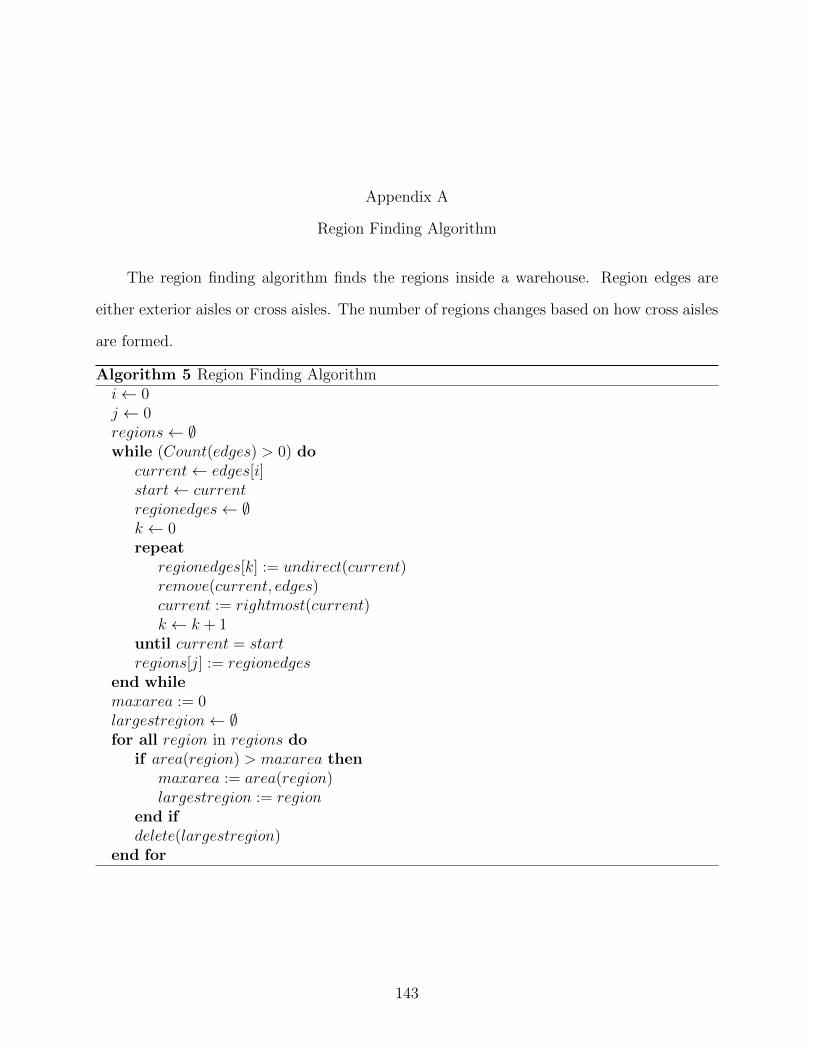
Appendix A

Region Finding Algorithm

The region finding algorithm finds the regions inside a warehouse. Region edges are

either exterior aisles or cross aisles. The number of regions changes based on how cross aisles

are formed.

Algorithm 5 Region Finding Algorithmi← 0j ← 0regions← ∅while (Count(edges) > 0) do

current← edges[i]start← currentregionedges← ∅k ← 0repeat

regionedges[k] := undirect(current)remove(current, edges)current := rightmost(current)k ← k + 1

until current = startregions[j] := regionedges

end whilemaxarea := 0largestregion← ∅for all region in regions do

if area(region) > maxarea thenmaxarea := area(region)largestregion := region

end ifdelete(largestregion)

end for

143