A Computer Aided Detection System For Digital Mammograms Based on Radial Basis Functions

and Feature Extraction Techniques

By Mohammed Jirari

Shanghai, China

Sept 3rd, 2005

Why This Project?

• Breast Cancer is the most common cancer and is the second leading cause of cancer deaths

• Mammographic screening reduces the mortality of breast cancer

• But, mammography has low positive predictive value PPV (only 35% have malignancies)

• Goal of Computer Aided Detection CAD is to provide a second reading, hence reducing the false positive rate

Basic Components of the System

• Preprocessing– Cropping

– Enhancement (Histogram Equalization)

• Feature extraction• Normalization• Training• Testing• ROC Analysis

What is a Mammogram?

• A Mammogram is an x-ray image of the breast. Mammography is the procedure used to generate a mammogram

• The equipment used to obtain a mammogram, however, is very different from that used to perform an x-ray of chest or bones

Mammograms (cont.)

• In order to get a good image, the breast must also be flattened or compressed

• In a standard examination, two images of each breast are taken: one from the top and

one from the side

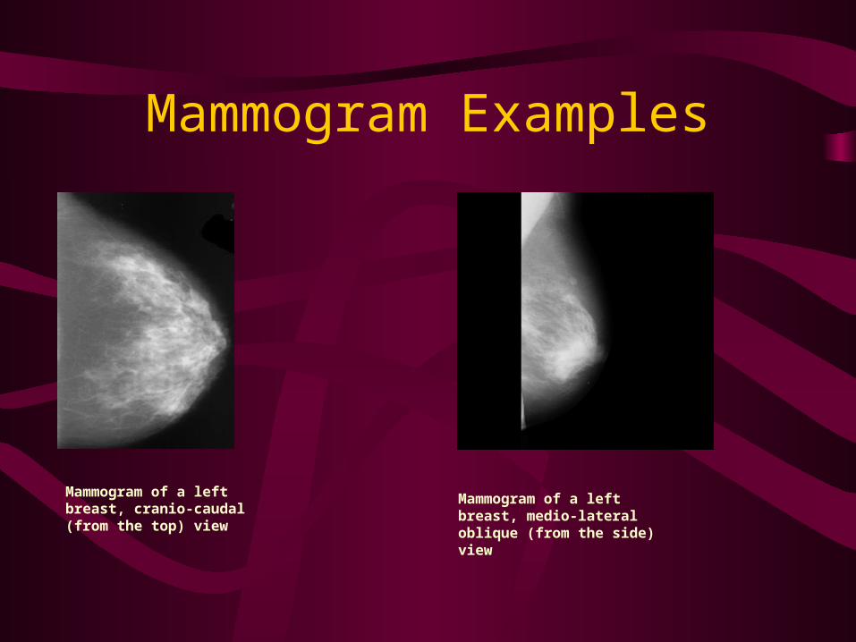
Mammogram Examples

Mammogram of a left breast, cranio-caudal (from the top) view

Mammogram of a left breast, medio-lateral oblique (from the side) view

Purpose of CAD

• Mammography is the most reliable method in early detection of breast cancer

• But, due to the high number of mammograms to be read, the accuracy rate tends to decrease

• Double reading of mammograms has been proven to increase the accuracy, but at high cost

• CAD can assist the medical staff to achieve high efficiency and effectiveness

• The physician/radiologist makes the call not CAD

Proposed Method

• The proposed method will assist the physician by providing a second opinion on reading the mammogram, by pointing out an area (if one exists) delimited by its center coordinates and its radius

• If the two readings are similar, no more work is to be done

• If they are different, the radiologist will take a second look to make the final diagnosis

Data Used

• The dataset used is the Mammographic Image Analysis Society (MIAS) MINIMIAS database containing Medio-Lateral Oblique (MLO) views for each breast for 161 patients for a total of 322 imagesEach image is: 1024 pixels X 1024 pixels

Preprocessing

• Cropping: cuts the black parts of the image (almost 50%) based on a threshold

• Enhancement: Histogram equalization to accentuate the features to be extracted by increasing the dynamic range of gray levels

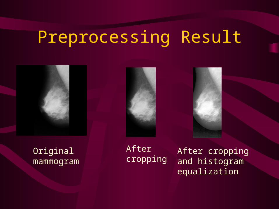
Preprocessing Result

Original mammogram

After cropping

After cropping and histogram equalization

Co-occurrence Matrices to Calculate Features

• The joint probability of occurrence of gray level a and b for two pixels with a defined spatial relationship in an image

• The spatial relationship is defined in terms of distance d and angle θ

• From these matrices, a variety of features may be extracted

Co-occurrence Matrices (cont.)

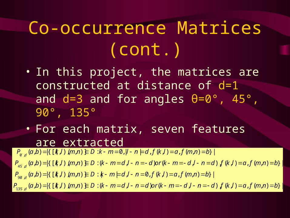
• In this project, the matrices are constructed at distance of d=1 and d=3 and for angles θ=0°, 45°, 90°, 135°

• For each matrix, seven features are extracted• Can be formally represented as follows:

|}),(,),(),,(),(:)],(),,{[(|),(

|}),(,),(,0,|:|)],(),,{[(|),(

|}),(,),(),,(),(:)],(),,{[(|),(

|}),(,),(,||,0:)],(),,{[(|),(

,135

,90

,45

,0

bnmfalkfdnldmkordnldmkDnmlkbaP

bnmfalkfnldmkDnmlkbaP

bnmfalkfdnldmkordnldmkDnmlkbaP

bnmfalkfdnlmkDnmlkbaP

d

d

d

d

Features Used

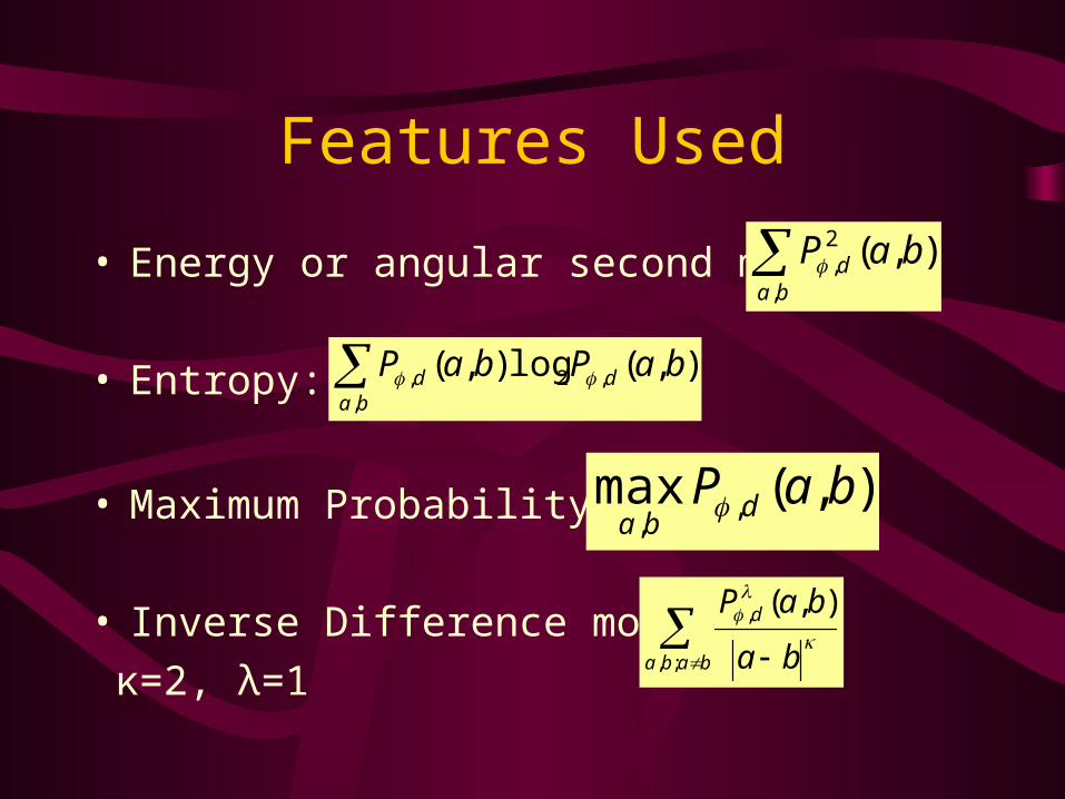
• Energy or angular second moment:

• Entropy:

• Maximum Probability:

• Inverse Difference moment:

κ=2, λ=1

ba

d baP,

2, ),(

),(log),( ,,

2, baPbaP dba

d

),(max ,,

baP dba

baba

d

ba

baP

;,

, ),(

Features Used (cont.)

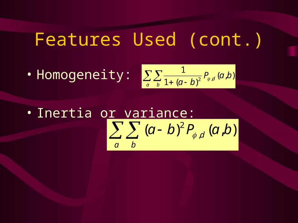
• Homogeneity:

• Inertia or variance:

a bd baP

ba),(

)(1

1,2

a b

d baPba ),()( ,2

Features Used (cont.)

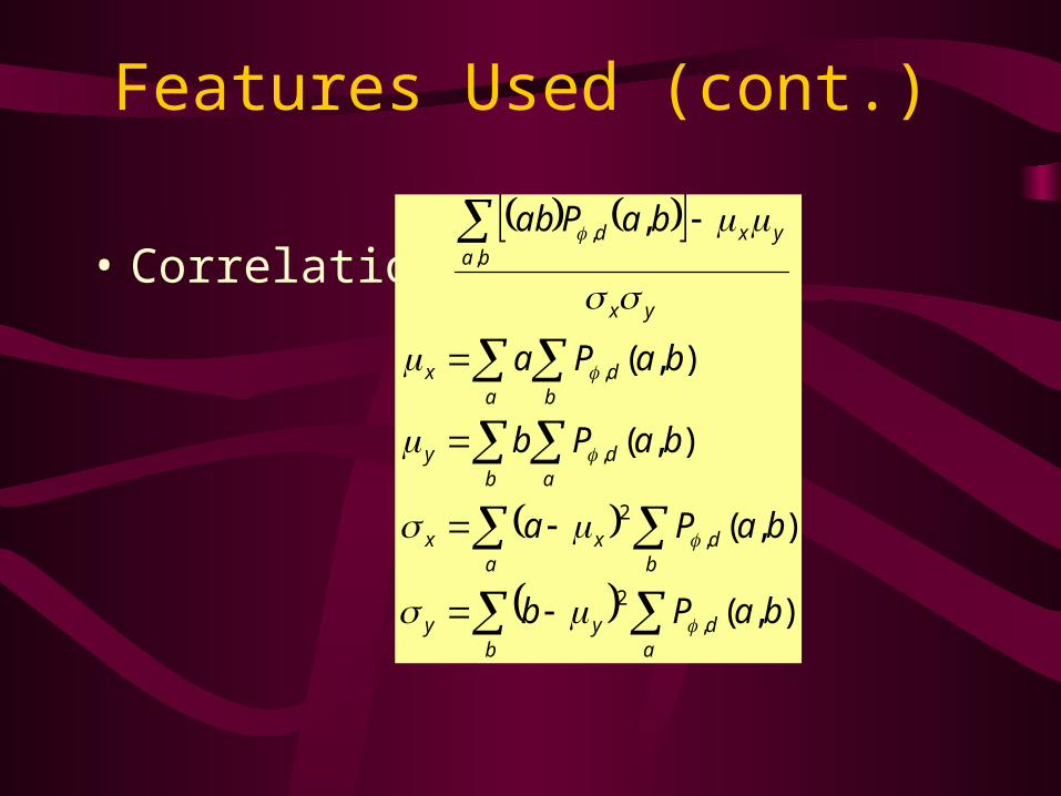
• Correlation:

b adyy

a bdxx

b ady

a bdx

yx

yxba

d

baPb

baPa

baPb

baPa

baPab

),(

),(

),(

),(

,

,2

,2

,

,

,,

Feature Extraction

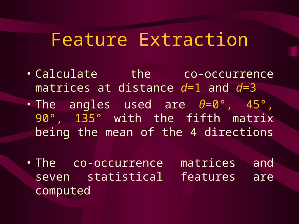
• Calculate the co-occurrence matrices at distance d=1 and d=3

• The angles used are θ=0°, 45°, 90°, 135° with the fifth matrix being the mean of the 4 directions

• The co-occurrence matrices and seven statistical features are computed

Example of Calculated Features

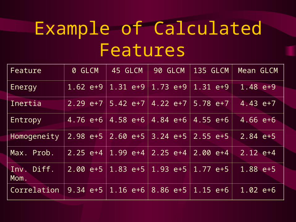
Feature 0 GLCM 45 GLCM 90 GLCM 135 GLCM Mean GLCM

Energy 1.62 e+9 1.31 e+9 1.73 e+9 1.31 e+9 1.48 e+9

Inertia 2.29 e+7 5.42 e+7 4.22 e+7 5.78 e+7 4.43 e+7

Entropy 4.76 e+6 4.58 e+6 4.84 e+6 4.55 e+6 4.66 e+6

Homogeneity 2.98 e+5 2.60 e+5 3.24 e+5 2.55 e+5 2.84 e+5

Max. Prob. 2.25 e+4 1.99 e+4 2.25 e+4 2.00 e+4 2.12 e+4

Inv. Diff. Mom. 2.00 e+5 1.83 e+5 1.93 e+5 1.77 e+5 1.88 e+5

Correlation 9.34 e+5 1.16 e+6 8.86 e+5 1.15 e+6 1.02 e+6

Radial Basis Network Used

• Radial basis networks may require more neurons than standard feed-forward backpropagation (FFBP) networks

• BUT, can be designed in a fraction of the time to train FFBP

• Work best with many training vectors

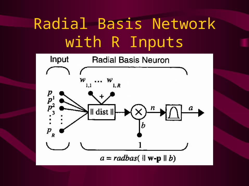
Radial Basis Network with R Inputs

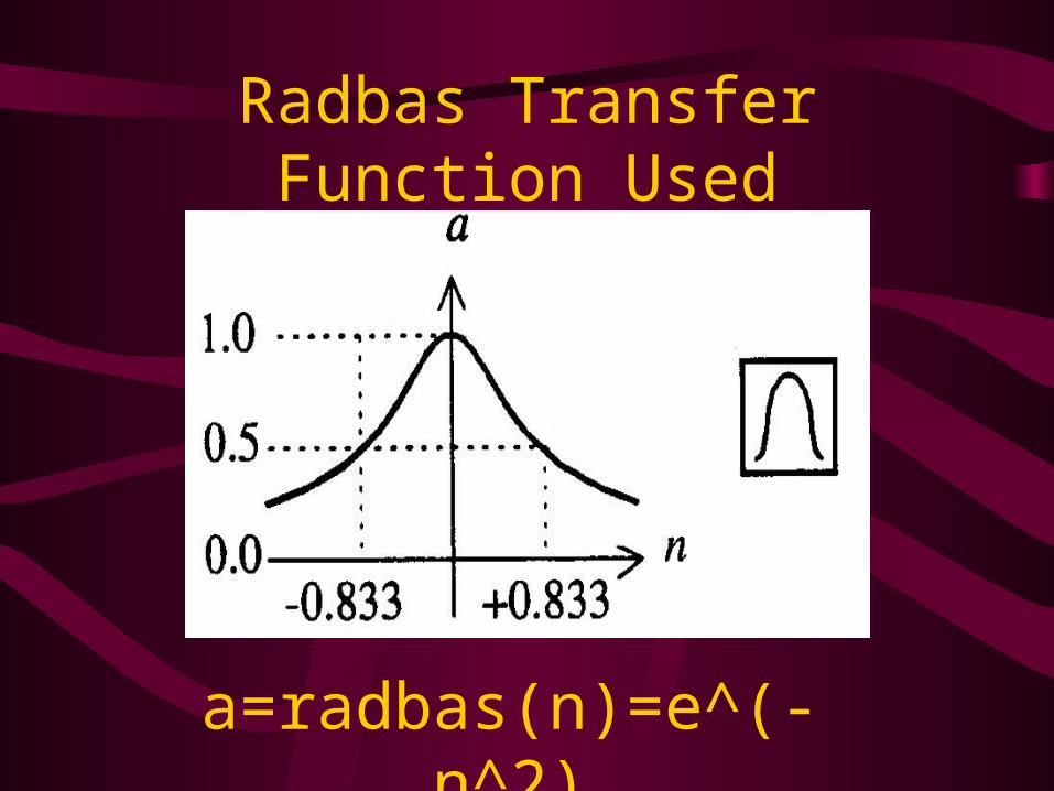
a=radbas(n)=e^(-n^2)

Radbas Transfer Function Used

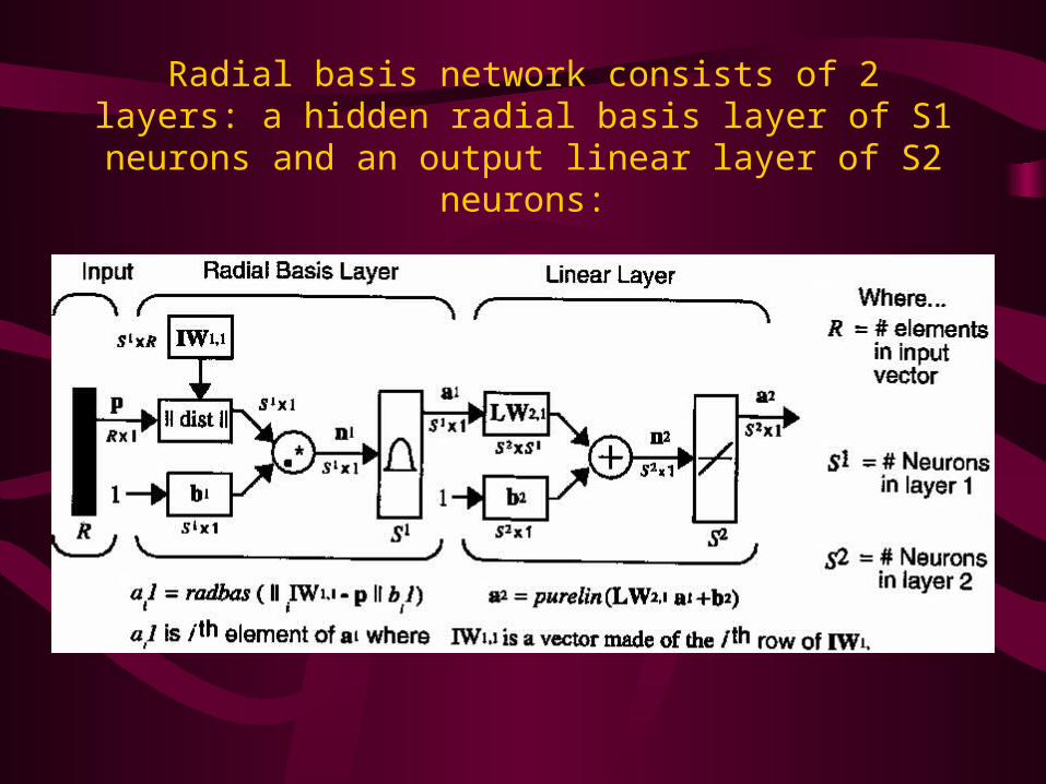
Radial basis network consists of 2 layers: a hidden radial basis layer of S1 neurons and an output linear layer of S2

neurons:

Training

• After normalizing the data, training begins

• The first training set was made up of 212 mammograms with 81 abnormal ones, with features calculated at distances d=1 and d=3

• The second training set was made up of 163 mammograms with 81 abnormal ones, with features calculated at distances d=1 and d=3

Testing

• A mammogram is presented to the trained network and the output is a suspicious area denoted by its center’s x and y coordinates and its radius. If the mammogram is considered to be normal then zeros are returned for the coordinates and radius

• The radiologist can then review his/her original assessment of the patient if some areas uncovered by the network were not originally looked at closely

• The whole database is tested and the accuracy is calculated• The smaller dataset performed better than the larger one,

and using d=3 leads to better results than d=1

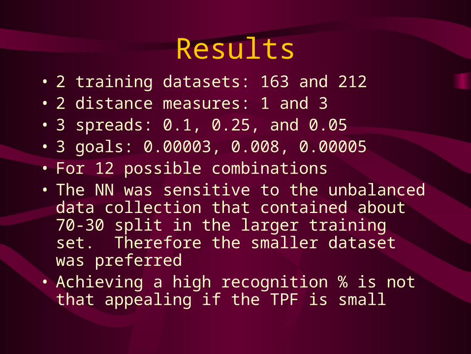
Results• 2 training datasets: 163 and 212• 2 distance measures: 1 and 3• 3 spreads: 0.1, 0.25, and 0.05• 3 goals: 0.00003, 0.008, 0.00005• For 12 possible combinations• The NN was sensitive to the unbalanced data

collection that contained about 70-30 split in the larger training set. Therefore the smaller dataset was preferred

• Achieving a high recognition % is not that appealing if the TPF is small

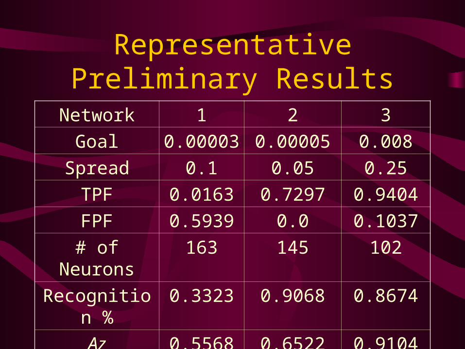
Representative Preliminary Results

Network 1 2 3

Goal 0.00003 0.00005 0.008

Spread 0.1 0.05 0.25

TPF 0.0163 0.7297 0.9404

FPF 0.5939 0.0 0.1037

# of Neurons 163 145 102

Recognition % 0.3323 0.9068 0.8674

Az 0.5568 0.6522 0.9104

Future work

• Use more features like standard deviation, skewness, and kurtosis

• Which feature(s) have the most impact:* Rank the features from best to worst (single

input to NN)* Select most significant feature(s) by using leave

one out method• Determine whether the area is benign or malignant

by adding the severity of the abnormality to the training

Future work (cont.)

• Try and reduce False Negatives on the basis of region characteristics size, difference in homogeneity and entropy

• Use larger database that contains both MLO and CC to train/learn, since most commercial CADs use hundreds of thousands of mammograms to try and recognize foreign samples

Thank you

Questions