A COMPUTER PROGRAM FOR SHORT CIRCUIT ANALYSIS OF …

NIJOTECH VOL. 5 NO. 1 MARCH 1981 EJEBE 46

A COMPUTER PROGRAM FOR SHORT CIRCUIT ANALYSIS OF ELECTRIC

POWER SYSTEMS

BY

G.C. EJEBE

DEPARTMENT OF ELECTRICAL/ELECTRONIC ENGINEERING

UNIVERSITY OF NIGERIA, NSUKKA.

(Manuscript received 23rd May 1980 and in revised form 10

th October 1980)

ABSTRACT

This paper described the mathematical basis and computational

framework of a computer program developed for short circuit studies of

electric power systems. The Short Circuit Analysis Program (SCAP) is to

be used to assess the composite effects of unbalanced and balanced faults

on the overall reliability of electric power system.

The program uses the symmetrical components method to compute all

phase and sequence quantities for any bus or branch of a given power

network resulting from the application of balanced and unbalanced faults

at any location of the system. The Key to the efficient computer

implementation of this program is the utilization of the triangular

factorization of the positive and zero sequence admittance matrices, thus

avoiding the time consuming direct formation of the sequence impedance

matrices.

INTRODUCTION

The purpose of short circuit

analysis of power systems is to

assess the vulnerability of the

system to abnormal conditions

resulting from a partial or

complete breakdown of insulation

at one or more points of the

system. Specifically in short

circuit studies, the power system

network is subjected to postulated

fault conditions and the resulting

faulted network is solved to

determine the phase (and sequence)

voltages, currents and power of

any bus or transmission line of

the system. From this analysis,

the power system engineer

determines the maximum and minimum

currents that are likely to result

from any of the array of available

fault conditions such as – single

line to ground fault (S – L – G

fault), double line to ground

fault (L – L – G fault), line – to

– line fault (L – l fault), or a

three – phase fault.

It is pertinent to state

that the information obtained from

short circuit analysis is an

effective tool for use in areas of

power system work such as system

design, relaying design and

disturbance review analysis. A

typical application of the

information obtainable from short

circuit analysis is in the

selection of circuit breakers of

appropriate interrupting capacity

to be installed in the protective

relay scheme for the power system.

Such power system protective

schemes in operation, are designed

to monitor the existence of a

fault in the system and promptly

initiate circuit breaker operation

to isolate the faulted part of the

power system from the rest of the

system. Thus a well deigned

protective scheme guarantees the

reliability and continuity of

supply in the remainder of the

power system in the event of

severe fault in one part of the

system. Another feasible

application of short circuit

analysis is in the realm of

disturbance review analysis in

which the calculation of the

actual phase currents and voltages

seen by the relays is needed to

determine whether they operated

correctly or in error in the event

of a major substation fault. From


the foregoing, it is obvious that

the need for a reliable short

circuit analysis of the power

system cannot be over-emphasized.

While many conventional

fault programs are limited to

output of phase quantities in the

close neighbourhood of the fault

point, the program presented here

provides for computation of

sequence and phase voltages and

currents at all points in the

power network. The mathematical

basis, program framework and

computational procedure as well as

an example of its application are

presented.

GENERAL PROGRAM DESCRIPTION

As it is usual in most short

circuit studies, some basic

assumptions are made to facilitate

the computational task of fault

analysis. These basic assumptions

are as follows [1]

(i) All load currents are

negligible.

(ii) All generated voltages are

equal in phase and magnitude

to the positive sequence

pre-fault voltage.

(iii) The networks are balanced

except at the fault points.

(iv) All shunt admittances (line

charging susceptance, etc.)

are negligible.

These basic simplifications have

not been made in developing the

program. Specifically the program

developed includes explicit

treatment of:

(a) Resistance, reactance and

charging susceptance of all

transmission branches.

(b) Loads represented as shunt

admittances to ground.

(c) Generator internal voltage are set at actual magnitudes and

phases as computed by a base

case load flow.

In order to save computer

storage, the program assumes that

the positive and negative sequence

networks are identical, and hence

only one is stored.

The solution of power system

networks under fault conditions

requires the elements of the

driving point impedance matrix Z.

Presently, two approaches [2] have

been developed for obtaining the

driving point impedance (or short

circuit impedance) matriz Z. The

first approach employs a building

algorithm [2] for the direct

formation of the impedance matrix.

However this method has been found

to be more difficult and time

consuming. The second approach

first forms the power system bus

admittance matrix Y and then

inverts this matrix to obtain the

driving point impedance matrix Z.

Conventionally to obtain the

inverse of the admittance matrix,

Gaussian elimination or Crout's

method [3] are used. However these

techniques require all elements of

the admittance matrix throughout

the execution. The program

described here, makes use of

matrix triangular factorization

which today is widely applied as

one of the powerful analytical

tools, especially to load flow

problems [4]. In this method, the

admittance matrix is first formed

and stored in a sparse triangular

factored form, from which the

short circuit impedance matrix is

obtained by backward substitution.

PROGRAM DEVELOPMENT

The short circuit analysis

program SCAP uses the symmetrical

component representation of the

power transmission network. The

effect of unbalanced faults is to

produce interconnections between

the three sequence networks - the

positive sequence, negative

sequence and zero sequence

networks, thus creating a new

composite network which contains

as many modes as the positive

sequence network. The

interconnections of sequence

networks for a wide range of

faults have been well documented

[5,1]. The short circuit analysis

program must solve this composite

network for the bus voltage, given

the base case load flow generator

voltages. The mathematical

formulation and solution of two

common unbalanced faults are shown

in the Appendix. The program takes


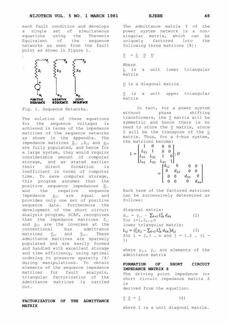
each fault condition and develops

a single set of simultaneous

equations using the Thevenin

Equivalent of the sequence

networks as seen from the fault

point as shown in figure 1.

Fig. 1. Sequence Networks.

The solution of these equations

for the sequence voltages is

achieved in terms of the impedance

matrices of the sequence networks

as shown in the Appendix. The

impedance matrices Z11 ,Z22 and z00

are fully populated, and hence for

a large system, they would require

considerable amount of computer

storage, and as stated earlier

their direct formation is

inefficient in terms of computer

time. To save computer storage,

this program assumes that the

positive sequence impedances Z11

and the negative sequence

Impedance z22 are equal and

provides only one set of positive

sequence data. Furthermore the

development of the short circuit

analysis program, SCAP, recognizes

that the impedance matrices Z11

and z00 are the inverses at the

conventional bus admittance

matrices Y22 and Y00. These

admittance matrices are sparsely

populated and are easily formed

and handled with excellent storage

and time efficiency, using optimal

ordering to preserve sparsity /4/

during manipulations. To obtain

elements of the sequence impedance

matrices for fault analysis,

triangular factorization of the

admittance matrices is carried

out.

FACTORIZATION OF THE ADMITTANCE

MATRIX

The admittance matrix Y of the

power system network is a non-

singular matrix, which can be

uniquely factored into the

following three matrices [8]:

Y = L D U

Where

L is a unit lower triangular

matrix

D is a diagonal matrix

U is a unit upper triangular

matrix

In fact, for a power system

without phase shifting

transformers, the Y matrix will be

symmetric and hence there is no

need to store the U matrix, since

U will be the transpose of the L

matrix. Thus, for a 4-bus system,

the matrices become:

[

]

[

]

Each term of the factored matrices

can be successively determined as

follows:

diagonal matrix:

dii = yii – ∑

(2)

for i=1,2,…,n

lower triangular matrix:

( ∑

) (3)

for i = 2,3 … n and j = 1.2 … (i -

1)

where yij, yii are elements of the

admittance matrix

FORMATION OF SHORT CIRCUIT

IMPEDANCE MATRIX Z

The driving point impedance (or

short circuit impedance matrix Z

is

derived from the equation:

Y Z = I (4)

where I is a unit diagonal matrix.


Replacing the admittance matrix by

its factors we have:

L D Lt Z = I (5)

If we define a transition matrix G

by

G = [L D]-1 = (6)

then since L-1 is a lower

triangular matrix and. D-1 is a

diagonal matrix, the transition

matrix G is also a lower

triangular matrix with its

diagonal terms given by:

; i=1, 2, …, n (7)

Furthermore we define a transfer

matrix,

T = I - Lt (8)

which is a strictly upper

triangular matrix with zero

diagonal terms.

Substituting equations (8)

and (6) into (5), a simplified

expression for the impedance

matrix Z results as follows:

Z = G + T Z (9)

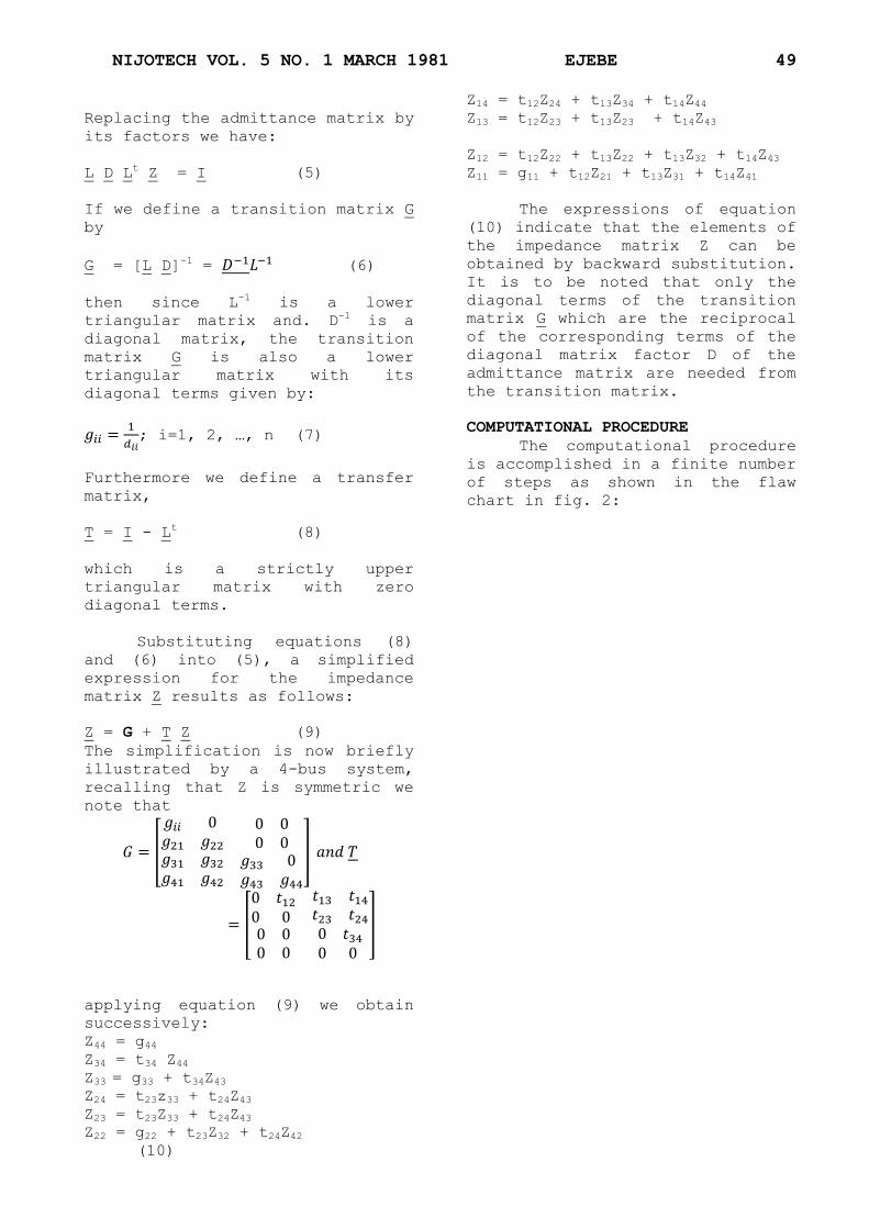
The simplification is now briefly

illustrated by a 4-bus system,

recalling that Z is symmetric we

note that

[

]

[

]

applying equation (9) we obtain

successively:

Z44 = g44

Z34 = t34 Z44 Z33 = g33 + t34Z43 Z24 = t23z33 + t24Z43 Z23 = t23Z33 + t24Z43

Z22 = g22 + t23Z32 + t24Z42

(10)

Z14 = t12Z24 + t13Z34 + t14Z44

Z13 = t12Z23 + t13Z23 + t14Z43

Z12 = t12Z22 + t13Z22 + t13Z32 + t14Z43

Z11 = g11 + t12Z21 + t13Z31 + t14Z41

The expressions of equation

(10) indicate that the elements of

the impedance matrix Z can be

obtained by backward substitution.

It is to be noted that only the

diagonal terms of the transition

matrix G which are the reciprocal

of the corresponding terms of the

diagonal matrix factor D of the

admittance matrix are needed from

the transition matrix.

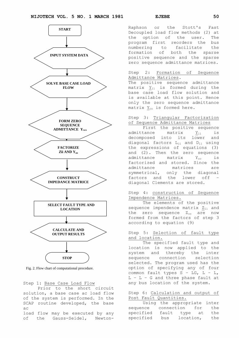
COMPUTATIONAL PROCEDURE

The computational procedure

is accomplished in a finite number

of steps as shown in the flaw

chart in fig. 2:


Step 1: Base Case Load Flow

Prior to the short circuit

solution, a base case ac load flow

of the system is performed. In the

SCAP routine developed, the base

ac

load flow may be executed by any

of the Gauss-Seidel, Newton-

Raphson or the Stott's Fast

Decoupled load flow methods (2) at

the option of the user. The

program first reorders the bus

numbering to facilitate the

formation of both the sparse

positive sequence and the sparse

zero sequence admittance matrices.

Step 2: Formation of Sequence

Admittance Matrices.

The positive sequence admittance

matrix Y11 is formed during the

base case load flow solution and

is available at this point. Hence

only the zero sequence admittance

matrix Yoo is formed here.

Step 3: Triangular Factorization

of Sequence Admittance Matrices

First the positive sequence

admittance matrix Y11 is

decomposed into its lower and

diagonal factors L11 and D11 using

the expressions of equations (3)

and (2). Then the zero sequence

admittance matrix Yoo is

factorized and stored. Since the

admittance matrices are

symmetrical, only the diagonal

factors and the lower off –

diagonal Clements are stored.

Step 4: construction of Sequence

Impendence Matrices.

The elements of the positive

sequence impendence matrix Z11 and

the zero sequence Zoo are now

formed from the factors of step 3

according to equation (9)

Step 5: Selection of fault type

and location.

The specified fault type and

location is now applied to the

system and thereby the inter

sequence connection selection

selected. The program used has the

option of specifying any of four

common fault types S – LG, L – L,

L – L – G and three phase fault at

any bus location of the system.

Step 6: Calculation and output of

Post Fault Quantities.

Using the appropriate inter

sequence connection for the

specified fault type at the

specified bus location, the

INPUT SYSTEM DATA

START

SOLVE BASE CASE LOAD

FLOW

FACTORIZE

Zii AND Yoo

CONSTRUCT

IMPEDANCE MATRICE

ZII & ZOO

CALCULATE AND

OUTPUT RESULTS

SELECT FAULT TYPE AND

LOCATION

STOP

Fig. 2. Flow chart of computational procedure.

FORM ZERO

SEQUENCE

ADMITTANCE YOO


program solves and computes the

output conditions at the fault

buses. At the option of the user,

the program can also output any

bus voltages in phase or sequence

coordinates, transmission line

currents, and transmission line

complex power for the entire

system.

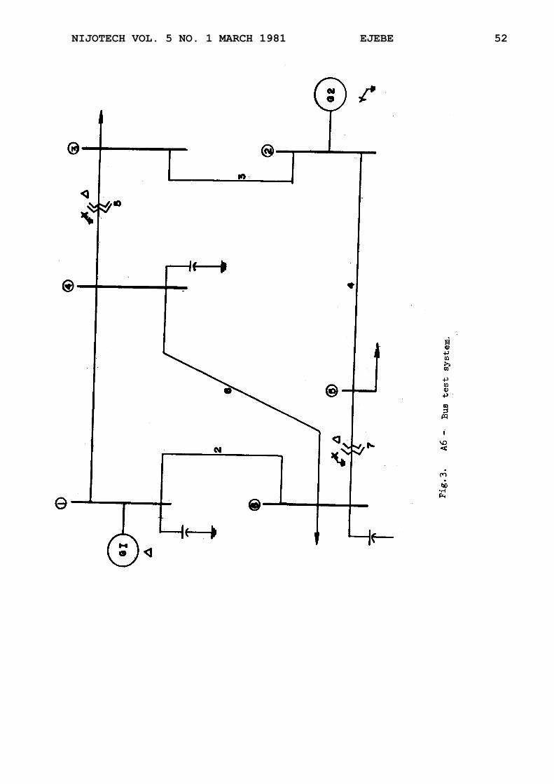
EXAMPLE APPLICAION

For an example of the program's

application the 6-bus system of

Ward and Hale [7] shown in Fig.3

is considered for two common

faults; a S-L-G, and a three-phase

fault at different buses of the

system. The system data includes

load data, and line shunt

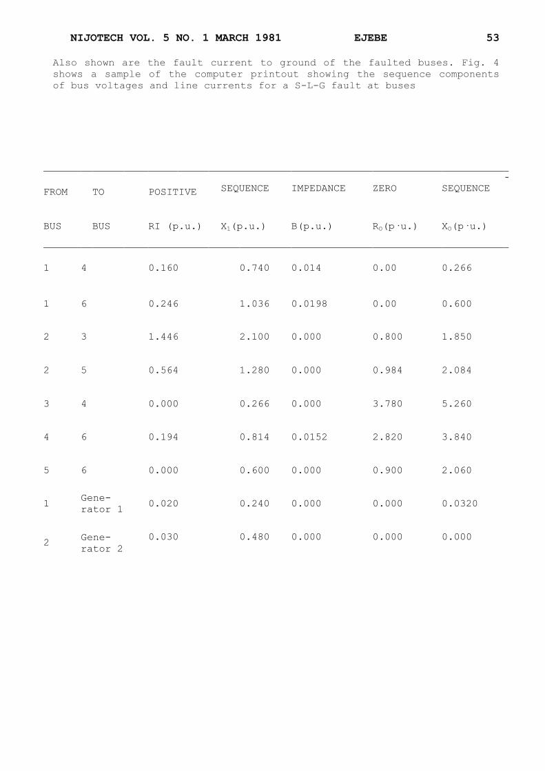
susceptance in addition to the

line, transformer and generator

impedances. The line impedance

data is given in per unit on a

system base of 100 MVA in Table 1.

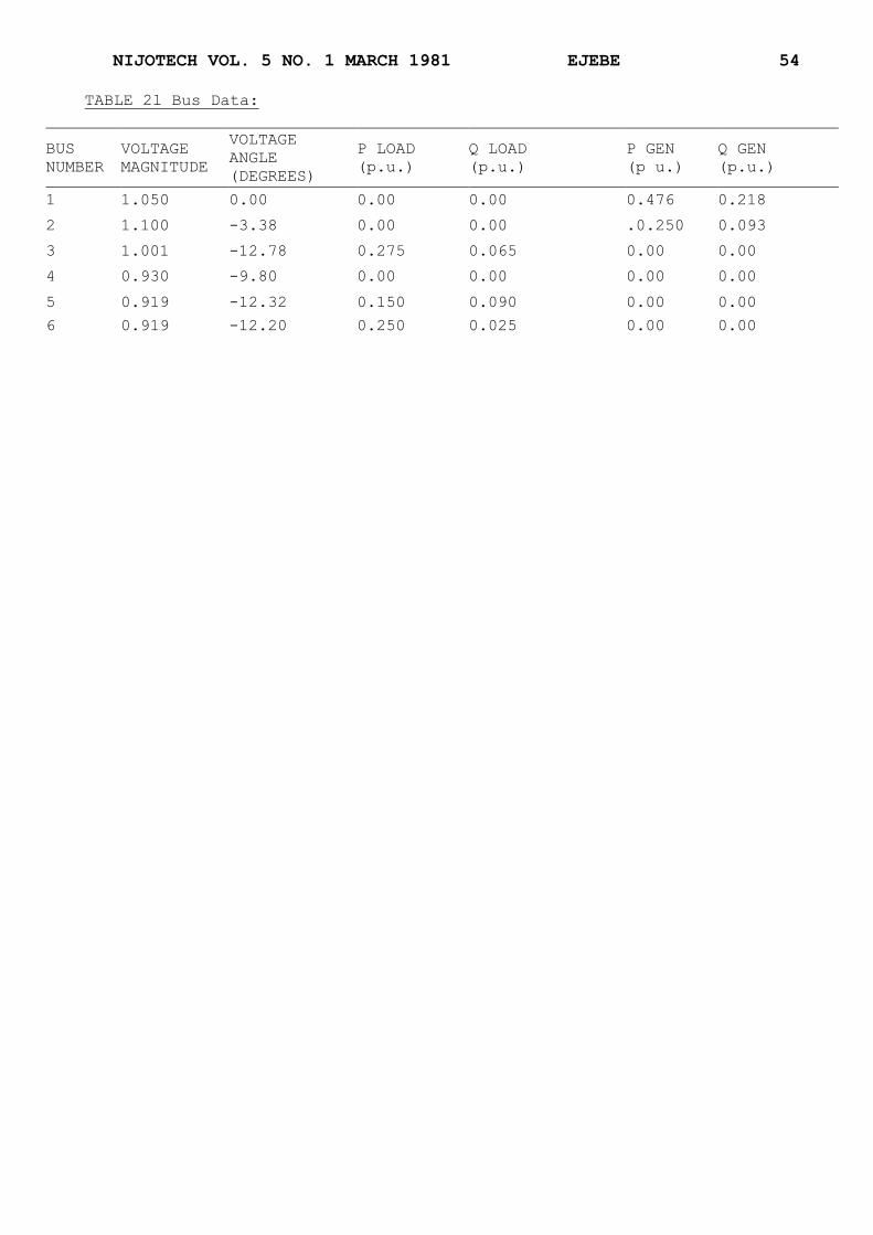
The bus load data with bas case

load flow voltages are given in

Table 2.

The computer results of the fault

study in terms of the post fault

bus voltages and transmission

circuit flows are compared against

the corresponding prefault

quantities for the S-L-G and

three- phase faults at buses 3 and

5 are shown in Tables 3 and 4 and

5 and 6 respectively.



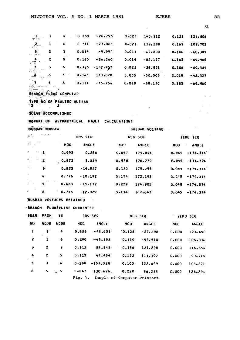
Also shown are the fault current to ground of the faulted buses. Fig. 4

shows a sample of the computer printout showing the sequence components

of bus voltages and line currents for a S-L-G fault at buses

SEQUENCE IMPEDANCE ZERO SEQUENCE

-

FROM TO POSITIVE

BUS BUS RI (p.u.) X1(p.u.) B(p.u.) RO(p·u.) XO(p·u.)

1 4 0.160 0.740 0.014 0.00 0.266

1 6 0.246 1.036 0.0198 0.00 0.600

2 3 1.446 2.100 0.000 0.800 1.850

2 5 0.564 1.280 0.000 0.984 2.084

3 4 0.000 0.266 0.000 3.780 5.260

4 6 0.194 0.814 0.0152 2.820 3.840

5 6 0.000 0.600 0.000 0.900 2.060

1 Gene-

rator 1 0.020 0.240 0.000 0.000 0.0320

2

Gene-

rator 2

0.030 0.480 0.000 0.000 0.000


TABLE 2l Bus Data:

BUS

NUMBER

VOLTAGE

MAGNITUDE

VOLTAGE

ANGLE

(DEGREES)

P LOAD

(p.u.)

Q LOAD

(p.u.)

P GEN

(p u.)

Q GEN

(p.u.)

1 1.050 0.00 0.00 0.00 0.476 0.218

2 1.100 -3.38 0.00 0.00 .0.250 0.093

3 1.001 -12.78 0.275 0.065 0.00 0.00

4 0.930 -9.80 0.00 0.00 0.00 0.00

5 0.919 -12.32 0.150 0.090 0.00 0.00

6 0.919 -12.20 0.250 0.025 0.00 0.00



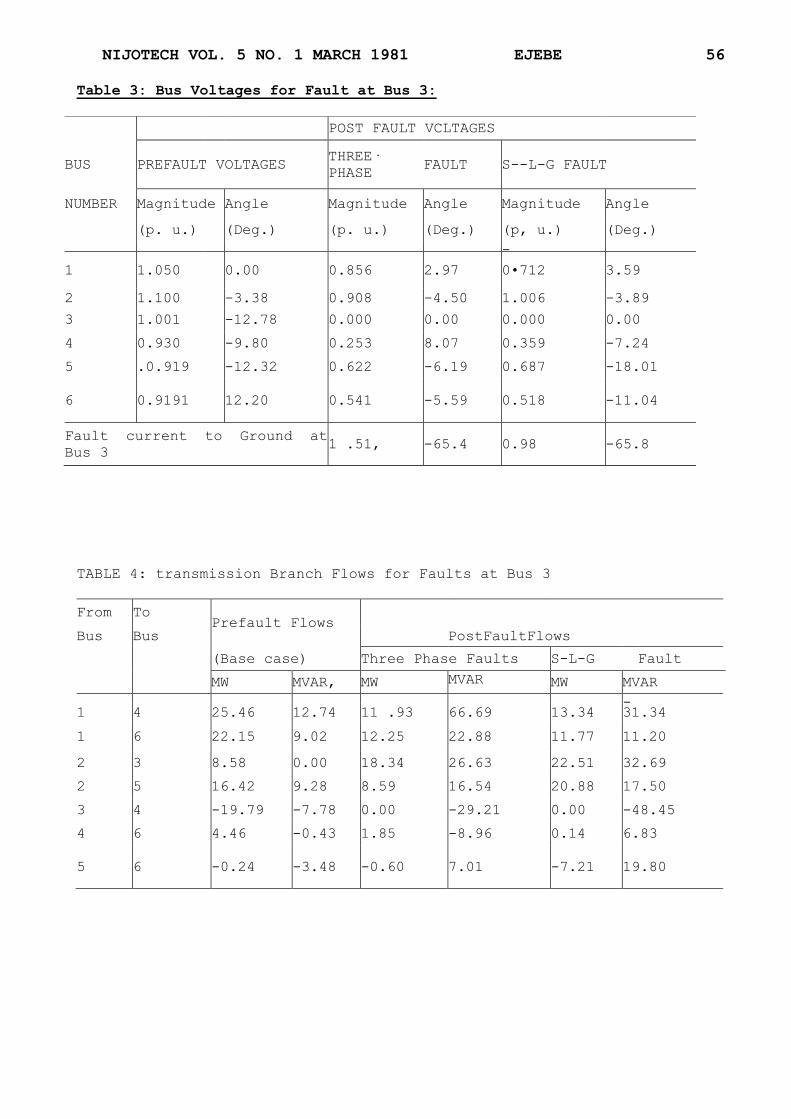
Table 3: Bus Voltages for Fault at Bus 3:

TABLE 4: transmission Branch Flows for Faults at Bus 3

POST FAULT VCLTAGES

BUS PREFAULT VOLTAGES THREE·

PHASE FAULT S--L-G FAULT

NUMBER Magnitude Angle Magnitude Angle Magnitude Angle

(p. u.) (Deg.) (p. u.) (Deg.) (p, u.) (Deg.)

-

1 1.050 0.00 0.856 2.97 0•712 3.59

2 1.100 -3.38 0.908 -4.50 1.006 -3.89

3 1.001 -12.78 0.000 0.00 0.000 0.00

4 0.930 -9.80 0.253 8.07 0.359 -7.24

5 .0.919 -12.32 0.622 -6.19 0.687 -18.01

6 0.9191 12.20 0.541 -5.59 0.518 -11.04

Fault current to Ground at

Bus 3 1 .51, -65.4 0.98 -65.8

From To Prefault Flows

Bus Bus PostFaultFlows

(Base case) Three Phase Faults S-L-G Fault

MW MVAR, MW MVAR

MW MVAR

- ,

1 4 25.46 12.74 11 .93 66.69 13.34 31.34

1 6 22.15 9.02 12.25 22.88 11.77 11.20

2 3 8.58 0.00 18.34 26.63 22.51 32.69

2 5 16.42 9.28 8.59 16.54 20.88 17.50

3 4 -19.79 -7.78 0.00 -29.21 0.00 -48.45

4 6 4.46 -0.43 1.85 -8.96 0.14 6.83

5 6 -0.24 -3.48 -0.60 7.01 -7.21 19.80


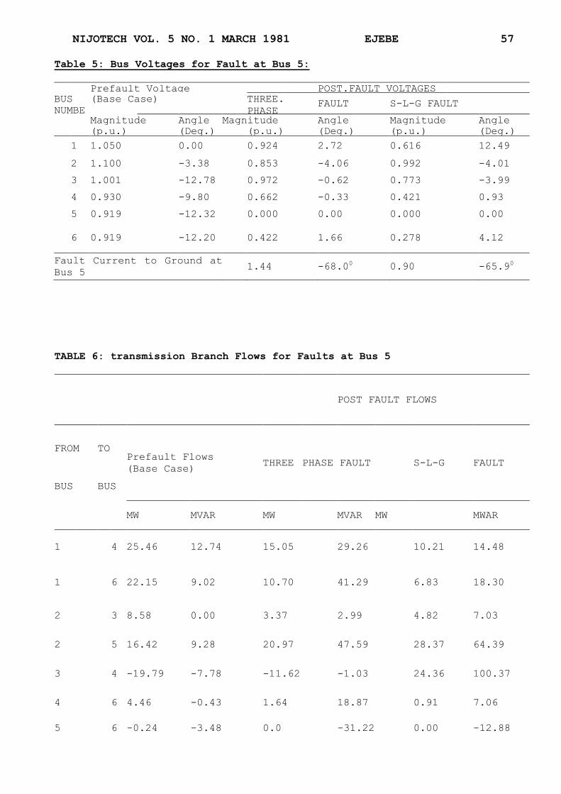
Table 5: Bus Voltages for Fault at Bus 5:

Prefault Voltage POST.FAULT VOLTAGES BUS (Base Case) THREE.

PHASE FAULT

S-L-G FAULT

NUMBE

R

Magnitude Angle Magnitude Angle Magnitude Angle

(p.u.) (Deg.) (p.u.) (Deg.) (p.u.) (Deg.)

1 1.050 0.00 0.924 2.72 0.616 12.49

2 1.100 -3.38 0.853 -4.06 0.992 -4.01

3 1.001 -12.78 0.972 -0.62 0.773 -3.99

4 0.930 -9.80 0.662 -0.33 0.421 0.93

5 0.919 -12.32 0.000 0.00 0.000 0.00

6 0.919 -12.20 0.422 1.66 0.278 4.12

Fault Current to Ground at

Bus 5 1.44 -68.0

0 0.90 -65.9

0

TABLE 6: transmission Branch Flows for Faults at Bus 5

POST FAULT FLOWS

FROM TO Prefault Flows

(Base Case) THREE PHASE FAULT

S-L-G FAULT

BUS BUS

MW MVAR MW MVAR MW MWAR

1 4 25.46 12.74 15.05 29.26 10.21 14.48

1 6 22.15 9.02 10.70 41.29 6.83 18.30

2 3 8.58 0.00 3.37 2.99 4.82 7.03

2 5 16.42 9.28 20.97 47.59 28.37 64.39

3 4 -19.79 -7.78 -11.62 -1.03 24.36 100.37

4 6 4.46 -0.43 1.64 18.87 0.91 7.06

5 6 -0.24 -3.48 0.0 -31.22 0.00 -12.88



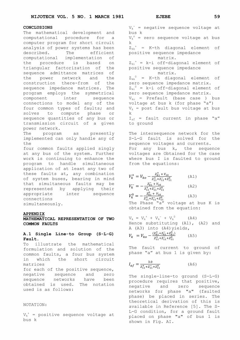
CONCLUSIONS

The mathematical development and

computational procedure for a

computer program for short circuit

analysis of power systems has been

described. The efficient

computational implementation of

the procedure is based on

triangular factorization of the

sequence admittance matrices of

the power network and the

construction there-from of the

sequence impedance matrices. The

program employs the symmetrical

component inter sequence

connections to model any of the

four common types of faults; and

solves to compute phase or

sequence quantities of any bus or

transmission circuit of a given

power network.

The program as presently

implemented can only handle any of

the

four common faults applied singly

at any bus of the system. Further

work is continuing to enhance the

program to handle simultaneous

application of at least any two of

these faults at, any combination

of system buses, bearing in mind

that simultaneous faults may be

represented by applying their

appropriate inter sequence

connections

simultaneously.

APPENDIX

MATHEMATICAL REPRESENTATION OF TWO

COMMON FAULTS

A.1 Single Line-to Group (S-L-G)

Fault.

To illustrate the mathematical

formulation and solution of the

common faults, a four bus system

in which the short circuit

matrices

for each of the positive sequence,

negative sequence and zero

sequence networks have been

obtained is used. The notation

used is as follows:

NOTATION:

Vk+ = positive sequence voltage at

bus k

Vk- = negative sequence voltage at

bus k

Vko = zero sequence voltage at bus

k

Zkk+ = K-th diagonal element of

positive sequence impedance

matrix.

Zki+ = k-i off-diagonal element of

positive sequence impedance

matrix.

Zkk0 = K-th diagonal element of

zero sequence impedance matrix.

Zki0 = k-i off-diagonal element of

zero sequence impedance matrix.

Vko = Prefault (base case ) bus

voltage at bus k (for phase “a”)

Vk = post fault bus voltage at bus

k

Iaf = fault current in phase “a”

to ground

The intersequence network for the

S-L-G fault is solved for the

sequence voltages and currents.

For any bus k, the sequence

voltages are Obtained for the case

where bus I is faulted to ground

from the equations:

(A1)

(A2)

(A3)

The Phase “a” voltage at bus K is

obtained from the equation:

Vk = Vk+ + Vk

- + Vk

0 (A4)

Hence substituting (A1), (A2) and

A (A3) into (A4)yields,

(A5)

The fault current to ground of

phase “a” at bus 1 is given by:

(A6)

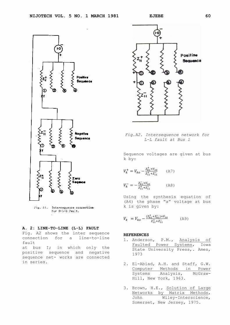
The single-line-to ground (S-L-G)

procedure requires that positive,

negative and zero sequence

networks for phase "a" (faulted

phase) be placed in series. The

theoretical derivation of this is

available in Reference [5]. The S-

L-G condition, for a ground fault

placed on phase "a" of bus 1 is

shown in Fig. AI.


A. 2: LINE-TO-LINE (L-L) FAULT

Fig. A2 shows the inter sequence

connection for a line-to-line

fault

at bus I; in which only the

positive sequence and negative

sequence networks are connected

in series.

Fig.A2. Intersequence network for

L-L fault at Bus 1

Sequence voltages are given at bus

k by:

(A7)

(A8)

Using the synthesis equation of

(A4) the phase “a” voltage at bus

k is given by:

(A9)

REFERENCES

1. Anderson, P.M., Analysis of

Faulted Power Systems, Iowa

State University Press,. Ames,

1973

2. El-Abiad, A.H. and Staff, G.W.

Computer Methods in Power

Systems Analysis, McGraw-

Hill, New York, 1963.

3. Brown, H.E., Solution of Large

Networks by Matrix Methods,

John Wiley-Interscience,

Somerset, New Jersey, 1975.


4. Ogbuogbiri, E.C. et al

"Sparsity-Directed

Decomposition for Gaussian

Elimination of Matrices", IEEE

Transactions on Power

Apparatus and Systems, Vol.

PAS 89, No.1, January 1968,

pp. I 4 I -I 49 .

5. Electrical Transmission and

Distribution Reference Book,

Westinghouse Corporation East

Pittsburgh, 1964.

6. Tinney, W.F. and Hart, C.E.,

"Power Flow Solution by

Newtons Method", IEEE

Transactions on Power

Apparatus & Systems, Vol.PAS

86; No.11, Nov.1967, pp ,

1449-1456.

7. Ward, J.B. and Hale H.W.,

"Digital Solution of Power

Flow Problem" Trans. A.I.E.E.,

75 pp.398-404, 1956.

8. Takahashi, K. et al,

"Formation of A Sparse Bus

Impedance

Matrix and its Application to

Short Circuit Study" IEEE PICA

Proceedings 1973,pp. 63-69.

Documents

A COMPUTER PROGRAM FOR SHORT CIRCUIT ANALYSIS OF …