Embed Size (px)
Citation preview
A Conceptual Design Methodology for Predicting the Aerodynamics ofUpper Surface Blowing on Airfoils and Wings
by:
Ernest B. Keen
Thesis submitted to the faculty ofVirginia Polytechnic Institute & State University
in partial fulfillment of the requirements for the degree of
Master of Science
in
Aerospace Engineering
APPROVED:
________________________________William H. Mason, Committee Chairman
________________________________Joseph A. Schetz
_________________________________Paul Gelhausen
November, 2004Blacksburg, Virginia
Keywords: Upper Surface Blowing, USB, aerodynamics, conceptual design, jet-flap

ii
A Conceptual Design Methodology for Predicting the Aerodynamics of UpperSurface Blowing on Airfoils and Wings
by:
Ernest B. Keen
(ABSTRACT)
One of the most promising powered-lift concepts is Upper Surface Blowing (USB),where the engines are placed above the wing and the engine exhaust jet becomes attachedto the upper surface. The jet thrust can then be vectored by use of the trailing edgecurvature since the jet flow tends to remain attached by the “Coanda Effect”. Wind tunneland flight-testing have shown USB aircraft to be capable of producing maximum liftcoefficients near 10. They have the additional benefit of shielding the engine noise abovethe wing and away from the ground.
Given the potential gains from USB aircraft, one would expect that conceptual designmethods exist for their development. This is not the case however. While relativelycomplex solutions are available, there is currently no adequate low-fidelity methodologyfor the conceptual and preliminary design of USB or USB/distributed propulsion aircraft.The focus of the current work is to provide such a methodology for conceptual design ofUSB aircraft. Based on limited experimental data, the new methodology is shown tocompare well with wind tunnel data.
In this thesis we have described the new approach, correlated it with available 2-Ddata, and presented comparisons of our predictions with published USB data and anexisting non-linear vortex lattice method. The current approach has been shown toproduce good results over a broad range of propulsion system parameters, winggeometries, and flap deflections. In addition, the semi-analytical nature of themethodology will lend itself well to aircraft design programs/optimizers such asACSYNT. These factors make the current method a useful tool for the design of USB andUSB/distributed propulsion aircraft.

iii
Acknowledgments
I would like first to thank my Lord, Jesus Christ, with whom everything is possible,and without whom I am nothing.
Also, I am more than grateful for the guidance and advise of my advisor, WilliamMason. His ideas and experience have saved me on many occasions, and he has taughtme more about practical engineering than anyone I’ve been around. It has been apleasure to be associated with him and his students.
To my family, Jack, Sheila, Jordan, I owe my thanks for years of love, support, openarms, and open ears. Their belief in me has pushed me to this point, and will drive me inthe years to come.
In addition, I would like to thank my friends at AVID, LLC for their funding andsupport of this research, and the friendships I can’t quantify. They have given meopportunities where there seemed to be none. I hope to represent them and theircommitment to excellence well with this work.
Lastly, I would like to thank my friends, here at Virginia Tech, back home, and out inthe wide,wide world. You’ve kept me sane, you’ve kept me laughing, and you’ve keptme going….and this is just the beginning.

iv
Table of Contents
Abstract……………………………………………………………………….. iiAcknowledgements…………………………………………………………… iiiTable of Contents……………………………………………………………... ivList of Figures………………………………………………………………….viList of Symbols………………………………………………………………... xi
Chapter 1, Introduction………………………………………………………….. 1
Chapter 2, Physics of Upper Surface Blowing………………………………… 52.1 Basic flow around an airfoil with no blowing……………………….. 62.2 Effects of trailing edge blowing………………………………………72.3 Effects of surface blowing…………………………………………… 142.4 Breakdown of forces………………………………………………… 172.5 Adverse effects………………………………………………………. 192.6 Three-Dimensional behavior…………...……………………………. 21
Chapter 3, Thrust/Drag Bookkeeping for USB Designs..…………………….. 233.1 Losses and bookkeeping…………………….………………………… 243.2 Estimating losses………………………………………………………. 26
Chapter 4, Development of a 2-D analytical method…………………………... 324.1 Basis for method/overview……………………………………………324.2 Spence’s jet-flap theory……………………………………………… 34
4.2.1 Lift Coefficient……………………………………………. 344.2.2 Pitching moment coefficient……………………………… 37
4.3 Circular Streamline Theory…………………………………………. 384.3.1 Derivation of CST for USB……………………………….. 404.3.2 Lift, Drag, and Pitching moment calculations…………….. 47
4.4 Drag estimation………………………………………………………494.5 Entrainment Effects…………………………………………………. 504.6 Total 2-D equations…………………………………………………. 51
4.6.1 Lift Coefficient…………………………………………….. 514.6.2 Pitching Moment Coefficient……………………………… 524.6.3 Drag Coefficient…………………………………………… 52
v
Chapter 5, Correlation of 2-D method with Experimental Data……………… 535.1 Description of Published Experiments………………………………..53
5.1.1 History and Overview………………………………………535.1.2 Experimental data………………………………………….. 56
5.2 Empirical factors and their physical basis……...……………………. 585.2.1 The “n” factor……………………………………………… 595.2.2 The “ηent” factor……………………………………………. 605.2.3 The pressure drag factor, ζ ..……………………………… 62
5.3 Presentation of 2-D correlation……………………………………… 635.3.1 Lift…………………………………………………………. 645.3.2 Pitching Moment……………………………………………675.3.3 Drag…………………………………………………………68
Chapter 6, Three-Dimensional USB Performance Prediction Method ……... 726.1 Overview of the Weissinger method…………………………………726.2 Using the new 2-D USB method with the Weissinger method ……. 75
6.2.1 The 2-D USB estimations…………………………………. 756.2.2 The High-Lift module………………………………………77
6.3 Limitations of method………………………………………………. 796.3.1 Spanload Oscillation……………………………………….. 806.3.2 Stall prediction……………………………………………...846.3.3 Nacelle and Fuselage effects………………………………. 85
6.4 Lateral-Directional Characteristics………………………………….. 86
Chapter 7, Comparison with 3-D experimental results………………………. 887.1 NASA Experimental USB Reports…………………………………. 89
7.1.1 Case 1: Small-scale, four-engine config. (TN 8061)………. 897.1.2 Case 2: Large-scale, twin-engine config. (TN 7526)……… 957.1.3 Case 3: Small-scale, four-engine config. (TN 7399)……… 104
7.2 YC-14 data…………………………………………………………...1097.3 Brief Comparison with a Non-Linear VLM……………………….. 114
Chapter 8, Conclusions/recommendations……………………………………… 120
References………………………………………………………………………….122
APPENDIX A: Annotated Bibliography……………………………………….. 127
APPENDIX B: Sample of Data Generation for 2-D Calculations……..……... 142
Vita………………………………………………………………………………… 146
vi
List of Figures
Figure Page
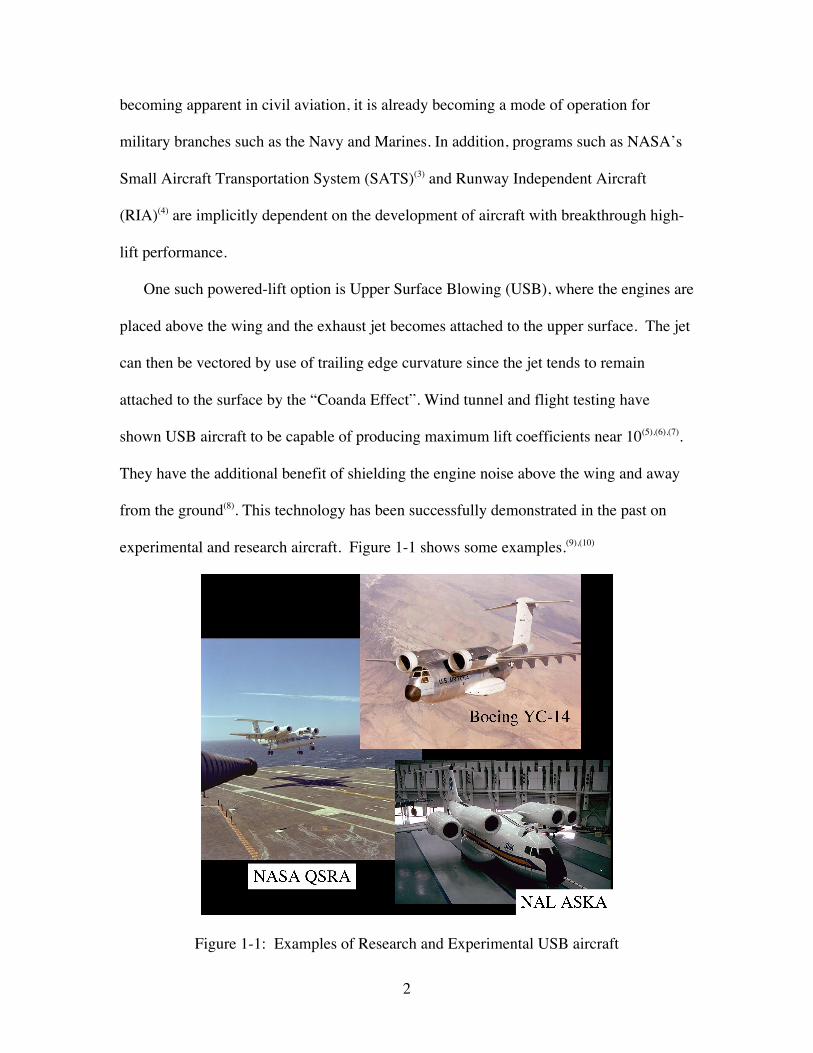
1-1 Examples of Research and Experimental USB aircraft…………………… 2
2-1 Forces on a flat plate in inviscid flow………………………………………7
2-2 Sketch of blown section with control surfaces…………………………….. 9
2-3 Pressure distribution on a jet-flapped airfoil from ref. 16…………………. 12
2-4 Sketch of the trailing edge of a jet-flapped airfoil…………………………. 12
2-5 USB configuration from Ref. 23……………………………………………14
2-6 YC-14 USB nacelle/nozzle/flap system…………………………………… 16
2-7 Sketch of forces for an idealized USB configuration……………………… 18
3-1 Thrust-plus-drag polars for a four-engine USB configurationat 35 deg flap deflection…………………………………………………….26
3-2 Sketch of nozzle exhaust flow angles……………………………………… 28
3-3 Comparison of experimental flow turning angle with empiricalrelation………………………………………………………………………29
3-4 Typical turning efficiency range for USB flap systems…………………….30
4-1 Schematic representation of the current method……………………………33
4-2 Agreement of dCL/dδf using derived approximate function……………….. 36
4-3 Example of the velocity profile of a wall jet flowing over a convexsurface with an external stream……………………………………………. 39
4-4 Streamlines and velocity profile produced by a point vortex……………… 40
4-5 Sketch of experimental setup used in ref. 24………………………………. 42
4-6 Comparison of CST with experimental data from ref 23………………….. 42
4-7 Sketch of actual and composite velocity profiles for a wall jet……………. 43
4-8 Comparison of CST with experimental data from ref 24………………….. 46
vii
4-9 Comparison of CST with static ground-test data from ref 8………………. 46
4-10 Comparison of CST with flight test data from ref 8……………………….. 47
4-11 Drawing of a USB surface discretized into small, linear segments……….. 48
5-1 Propulsive wing section used in experiments of ref 44……………………. 54
5-2 Sample of Cl vs. blowing coefficient from experiment……………………. 57
5-3 Sample of Cm, c/4 vs. Cl from experiment…………………………………… 57
5-4 Experimental data for pressure drag vs. blowing coefficient……………… 58
5-5 Pressure coefficients due to blowing effects………………………………. 60
5-6 2-D comparison of current method, Jet-flap theory, and experimentfor α=-5 degrees…………………………………………………………….64
5-7 2-D comparison of current method, Jet-flap theory, and experimentfor α=0 degrees……………………………………………………………. 65
5-8 2-D comparison of current method, Jet-flap theory, and experimentfor α=5 degrees……………………………………………………………..65
5-9 2-D comparison of current method, Jet-flap theory, and experimentfor α=10 degrees……………………………………………………………66
5-10 2-D comparison of current method, Jet-flap theory, and experimentfor α=15 degrees……………………………………………………………66
5-11 Comparison of Cm,c/4 for current method predictions and experiment………67
5-12 Comparison of Cm,c/4 for current method predictions and experiment………68
5-13 Correlation of pressure drag predictions for α=0 degrees…………………. 69
5-14 Correlation of pressure drag predictions for α=5 degrees…………………. 69
5-15 Correlation of pressure drag predictions for α=10 degrees………………... 70
5-16 Correlation of pressure drag predictions for α=15 degrees………………... 70
6-1 Vortex system representation of a lifting surface………………………….. 73

viii
6-2 Sample output data from MATLAB 2-D USB code………………………. 78
6-3 Planform view of wing used in experiments of ref 8……………………….81
6-4 Effective angle of attack across wing semi-span at α=20 deg…………….. 81
6-5 Wing-loading for the case shown in Figure 6-4…………………………….82
6-6 Original and corrected wing spanloadings………………………………….84
6-7 Sectional data regions across a wing for an engine-out case……………….86
7-1 Wing model of aircraft tested in ref 6………………………………………90
7-2 CL variation with alpha for 0 deg flaps at 2 thrust settings………………… 91
7-3 Pitching moment vs. alpha for 0 deg flaps at 2 thrust settings…………….. 92
7-4 Thrust-plus-drag polar for CT=0.9, 0 deg flaps……………………………..93
7-5 Thrust-plus-drag polar for CT=2.0, 0 deg flaps……………………………..93
7-6 CL variation with alpha for 35 deg USB flaps at 3 thrust settings…………. 94
7-7 Pitching moment about the C.G. for 35 deg USB flaps at3 thrust settings…………………………………………………………….. 94
7-8 Thrust-plus-drag polars for 35 deg USB flaps at 3 thrust settings………… 95
7-9 Wing planform used in experiments of ref 54……………………………. 96
7-10 CL variation with alpha for 0 deg flaps at 2 thrust settings………………… 97
7-11 CL variation with alpha for 20 deg flaps at 2 thrust settings……………….. 97
7-12 CL variation with alpha for 40 deg flaps at 2 thrust settings……………….. 98
7-13 CL variation with alpha for 60 deg flaps at 2 thrust settings……………….. 98
7-14 Example of induced drag correction for thrust-plus-drag polars…………...100
7-15 Thrust-plus-drag polars for 2 power settings at 0 deg flaps……………….. 100
7-16 Thrust-plus-drag polars for 2 power settings at 20 deg flaps……………….101
7-17 Thrust-plus-drag polars for 2 power settings at 40 deg flaps……………….101

ix
7-18 Thrust-plus-drag polars for 2 power settings at 60 deg flaps……………….102
7-19 Pitching moment about the aircraft C.G. vs. alpha for 0 deg flapsat 2 thrust settings………………………………………………………….. 103
7-20 Pitching moment about the aircraft C.G. vs. alpha for 20 deg flapsat 2 thrust settings………………………………………………………….. 103
7-21 Pitching moment about the aircraft C.G. vs. alpha for 40 deg flapsat 2 thrust settings………………………………………………………….. 104
7-22 Wing planform using in experiments of ref 55…………………………… 105
7-23 CL variation with alpha for 0 deg flaps at CT=2.16………………………… 106
7-24 Pitching moment about the aircraft C.G. vs. alpha for 0 deg flapsAt CT=2.16…………………………………………………………………. 106
7-25 Thrust-plus-drag polar for 0 deg flaps at CT=2.16…………………………. 107
7-26 CL variation with alpha for 35 deg flaps at 2 thrust settings……………….. 108
7-27 Thrust-plus-drag polars for 35 deg flaps at 2 thrust settings………………. 108
7-28 Pitching moment about the aircraft C.G. vs. alpha for 35 deg flapsat 2 thrust settings………………………………………………………….. 109
7-29 Wing planform for the Boeing YC-14…………………………………… 110
7-30 Upper surface profiles for various flap deflections…………………………111
7-31 CL variation with alpha for takeoff configuration at 2 thrust settings…….. 112
7-32 Thrust-plus-drag polars for takeoff configuration at 2 thrust settings……... 112
7-33 CL variation with alpha for landing configuration………………………… 113
7-34 Thrust-plus-drag polar for landing configuration………………………….. 114
7-35 CL predictions from VLM and current method for 45 deg deflectedradius flap at 2 thrust settings……………………………………………… 116

x
7-36 Pitching moments about the C.G. for 45 deg flaps at 2 thrust settings……. 117
7-37 Thrust-plus-drag polars for 45 deg flaps at 2 thrust settings………………. 117
7-38 Comparison of non-linear VLM to CST surface pressures ……………….. 118

xi
List of Symbols
b - wing span (ft)
b/2 - semi-span (ft)
bUSB - span of upper surface blowing (ft)c - local chord of airfoil (ft)
cf - chord of trailing edge flap (ft)
Cj,Cµ - sectional blowing coefficient/momentum flux coefficient =
€
˙ m VexitqcbUSB
Cl - sectional lift coefficient
CL - wing lift coefficientCLα - lift curve slope
Cd - sectional drag coefficient
Cdp - sectional pressure drag coefficientCDi - induced drag coefficient
CD - total drag coefficient
Cm - sectional pitching moment coefficient, about quarter-chordCM,cg - wing pitching moment coefficient about aircraft C.G. location
CT - total thrust coefficient of aircraft =
€
Total ThrustqS
CG - center of gravity of aircraft
e - span efficiency factor
E - ratio of flap chord to local airfoil chord =
€
c fc
h - height of nozzle exit (ft)
€
˙ m - engine mass flow rate (slug/s)
p∞ - freestream static pressure (lb/ft2)p - local static pressure (lb/ft2)
q∞ - freestream dynamic pressure (lb/ft2)qjet - dynamic pressure of jet (lb/ft2)
qi - 2-D vector from airfoil quarter chord to midpoint of ith panel
R - radius of curvature (ft)Rref - reference radial location (ft)

xii
r - radial location (ft)
Re - Reynolds numbersi - length of ith panel (ft)
S - wing planform area (ft2)t - engine exhaust jet thickness (ft)
t/c - thickness to chord ratio
V∞ - freestream velocity (ft/s)Vjet - engine exhaust jet velocity (ft/s)
x - chordwise coordinate in 2-D, origin at quarter-chord (ft)y - thickness coordinate in 2-D, origin at chord line (ft)
α - angle of attack (wing and airfoil) (rad)
αeff - effective angle of attack in 3-D (rad)
α0L - zero-lift angle of attack (rad)
χ - flap parameter =
€
2sin−1 E( )δf - flap deflection (rad)
δj - jet deflection (rad)
δeff - effective jet angle (includes trailing edge angle, turning efficiency) (rad)
γ - airfoil camber (% chord)
η - engine exhaust jet turning efficiency
ηent - empirical entrainment factor
λBLC - boundary layer control factor
µ - fluid viscosity (lb-s/ft2)
θi - local inclination of surface panel “i” (rad)
θTE - trailing edge angle of airfoil (rad)
θkd - nozzle “kick-down” angle (rad)
ρ∞ - freestream density (slug/ft3)
ρjet - jet density (slug/ft3)
τ - jet deflection angle for a pure jet flap (rad)
ζ - pressure drag factor, empirical multiplier
1
Chapter 1: Introduction
As modern aircraft have grown in size and complexity to become more cost efficient
for operators, so too has the infrastructure needed to accommodate them. Programs such
as the Airbus A380, which will carry over 800 passengers but only operate out of 60
airports worldwide(1), will do little to relieve this trend. This has placed huge demands on
the current “hub-and-spoke” airport system. With a limited throughput on major runways,
huge delays are often experienced. Such was the recent case at Chicago’s O’Hare airport
where delays reached critical limits, reducing the on-time arrivals in the whole air system
by 15%(2). Hundreds of millions of dollars are lost due to air traffic delays while adjacent
“stub” runways go unused and smaller regional airports operate at small fractions of their
capacity.
Why is the air system consistently pushed to its limits? Because there are no aircraft
in service that can meet the performance demands associated with short-field operations.
Clearly, there is a need for powered-lift aircraft that can demonstrate exceptional takeoff
and landing performance. While the need for Short Takeoff and Landing (STOL) is
2
becoming apparent in civil aviation, it is already becoming a mode of operation for
military branches such as the Navy and Marines. In addition, programs such as NASA’s
Small Aircraft Transportation System (SATS)(3) and Runway Independent Aircraft
(RIA)(4) are implicitly dependent on the development of aircraft with breakthrough high-
lift performance.
One such powered-lift option is Upper Surface Blowing (USB), where the engines are
placed above the wing and the exhaust jet becomes attached to the upper surface. The jet
can then be vectored by use of trailing edge curvature since the jet tends to remain
attached to the surface by the “Coanda Effect”. Wind tunnel and flight testing have
shown USB aircraft to be capable of producing maximum lift coefficients near 10(5),(6),(7).
They have the additional benefit of shielding the engine noise above the wing and away
from the ground(8). This technology has been successfully demonstrated in the past on
experimental and research aircraft. Figure 1-1 shows some examples.(9),(10)
Figure 1-1: Examples of Research and Experimental USB aircraft
3
Given the potential performance gains from USB aircraft, one would expect that
conceptual design methods exist for their development. However, this is not the case.
There is currently no low-fidelity methodology for the conceptual and preliminary design
of USB or USB/distributed propulsion aircraft. This can discourage a conceptual design
from making the transition to powered-lift. It has been stated that “90% of the cost of a
product is committed during the first 10% of the design cycle”.(11) It is easy to see the
importance of providing good estimations of performance at early design stages. Given
the inherent sensitivity of a USB design to high-lift performance, good estimations can
mean big savings in the design process.
The current state-of-the-art for 3-D USB predictions are zonal methods based on
coupling the Navier-Stokes equations with a potential flow panel method(12). However,
this is a complicated, high-fidelity model and cannot reasonably be implemented until the
detail design phase. Low-fidelity models have changed very little from those established
in the 1970s. Inviscid solutions using panel methods can be quite useful but require more
geometry detail, typically require an iterative solution for the jet boundaries, and cannot
predict drag. The most successful panel method was produced by Mendenhall(13) using a
non-linear vortex lattice formulation. A comparison of this method to the proposed
methodology is presented in this work. The classic “Jet-Flap” theory given by Spence(14)
is easy to use but, as will be shown in the chapters that follow, is inadequate for USB
predictions.
The purpose of the current work is to provide a low-fidelity performance prediction
methodology for Upper Surface Blown wings suited to use in the conceptual design
phase. This methodology will be demonstrated to have appropriate accuracy for early

4
design phases. It is also fast, easy to use, and robust enough to handle nearly all USB
configurations. Its ease of use will allow it to be integrated readily into existing aircraft
design programs. Table 1-1 shows a comparison of various methods for USB
performance calculations.
Table 1-1: Comparison of USB prediction methods
Low-fidelity? Accurate? Fast? Easy to Use / Easy tointegrate?
Coupled N-S /potential flow Panel methods Jet-Flap theory
Proposed method
The purpose of this work is to introduce a new approach for analyzing the problem, to
correlate it with 2-D data, and then extend it to 3-D performance predictions. The focus
is directed towards providing the methodology for low-fidelity USB performance
predictions. In addition, this work contains a description of a thrust-drag bookkeeping
method for USB designs. Also included is an annotated bibliography of a large number
of papers on the subject. The work contained in this thesis will be valuable for engineers
pursuing design concepts incorporating USB and USB/distributed-propulsion.

5
Chapter 2: Physics of Upper Surface Blowing
The changes induced in a flowfield when blowing is introduced can be dramatic. The
various effects have been documented to different degrees by previous researchers.
However, a broad, qualitative explanation of the total process has yet to be given. This is
due primarily to two things. First, there is a relatively small base of experimental data
upon which to draw conclusions. This is further complicated by the fact that most
experimental data is “configuration dependent”, meaning that generally a specific aircraft
configuration was tested. Thus, the basic physics can sometimes become obscured.
Second, this area of research hasn’t received much attention for some time.
It is the goal of this chapter to examine the effects of blowing on the flowfield around
an airfoil, with our particular interest being upper surface blowing. Some of the
phenomena involved are well understood, while others are not. In the latter cases,
possible explanations are offered with their basis in aerodynamic theory and published
experimental data.

6
2.1 - Basic Flow around an Airfoil with no blowing
Consider an airfoil immersed in an inviscid, uniform, steady flow. The body will
generate a circulation value specified by the enforcement of the Kutta condition at the
trailing edge. The Kutta-Joukowski theorem:
€
L = ρUΓ (2-1)
says that the lift is uniquely determined by the freestream conditions and the circulation.
Therefore, the greater the circulation, the greater the lift generated. The appropriate value
for the circulation is determined by the Kutta condition, since potential flow gives an
infinite number of possible solutions. The Kutta condition simply states that at a finite
angle trailing edge there must be a stagnation point, or for a cusped trailing edge, the
upper and lower velocities must be parallel and equal.
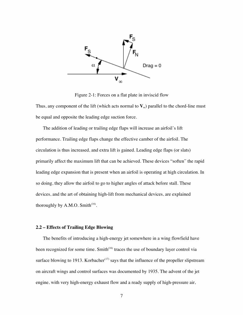
Equation (2-1) requires that the lift force be perpendicular to the freestream regardless
of the orientation of the airfoil. Thus, the drag for inviscid analysis must be zero. This
phenomenon is explained by Mason(15) as being a result of the leading-edge suction force.
This force is a result of the rapid expansion the flow experiences around the leading edge.
It becomes more pronounced as the stagnation point moves and it produces a forward
force parallel to the chord line. Consider Figure 2-1 from Mason(15) showing a flat plate
airfoil at a given angle of attack in an inviscid, attached flow.
7
Figure 2-1: Forces on a flat plate in inviscid flow
Thus, any component of the lift (which acts normal to V∞) parallel to the chord-line must
be equal and opposite the leading edge suction force.
The addition of leading or trailing edge flaps will increase an airfoil’s lift
performance. Trailing edge flaps change the effective camber of the airfoil. The
circulation is thus increased, and extra lift is gained. Leading edge flaps (or slats)
primarily affect the maximum lift that can be achieved. These devices “soften” the rapid
leading edge expansion that is present when an airfoil is operating at high circulation. In
so doing, they allow the airfoil to go to higher angles of attack before stall. These
devices, and the art of obtaining high-lift from mechanical devices, are explained
thoroughly by A.M.O. Smith(16).
2.2 – Effects of Trailing Edge Blowing
The benefits of introducing a high-energy jet somewhere in a wing flowfield have
been recognized for some time. Smith(16) traces the use of boundary layer control via
surface blowing to 1913. Korbacher(17) says that the influence of the propeller slipstream
on aircraft wings and control surfaces was documented by 1935. The advent of the jet
engine, with very high-energy exhaust flow and a ready supply of high-pressure air,
8
opened a world of possibilities for powered lift. Methods for analyzing jet-flapped
airfoils were developed by Spence(14) in the mid 1950s. General analytical methods for
wing-jet interaction of various basic configurations were then presented by Lan(18) and
Shollenberger(19) in the early 1970s.
For this work, the use of the term “blowing” will refer to either blowing from the
trailing edge or blowing across the upper surface of a wing or airfoil. There are certainly
other types of blowing, but the fundamental interactions are similar. At this point it is
also critical to establish our correlating parameter, the “blowing coefficient” or “jet
momentum coefficient”:
€
Cµ = C j =˙ m V jet
q∞c(2-2)
where the numerator is the gross thrust of a propulsion system operating at or near design
condition (jet static pressure equal to ambient pressure). This parameter is a measure of
the strength of the jet.
A distinction should also be made between blowing for boundary layer control and
for powered lift. Boundary layer control is the process of blowing to prevent boundary
layer separation. It typically uses very small amounts of air. As we begin to use more air,
the jet leaves the trailing edge with some small amount of momentum. At this point, call
it Cµ,crit, the boundary layer control has become powered lift. The increase in airfoil
circulation due to the jet is called “super-circulation”. There are two ways in which
blowing will alter the performance of an airfoil:
1. Through the direct reaction of jet momentum leaving the trailing edge.2. Through the change in airfoil circulation induced by the jet, i.e. through the
changes induced in the surface pressures around the airfoil.
9
The first is obvious, while the second, as we will show, can be complicated. It involves
many separate effects that are dependent on a wide array of flow features.
We begin with a discussion of trailing edge blowing. If this jet can be directed
downward, it is called a “jet-flap” and has been the subject of a great deal of analysis,
most notably that done by Spence(14). It is helpful to re-derive the Kutta-Joukowski
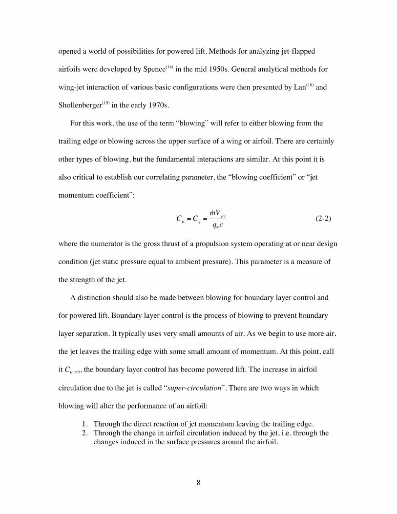
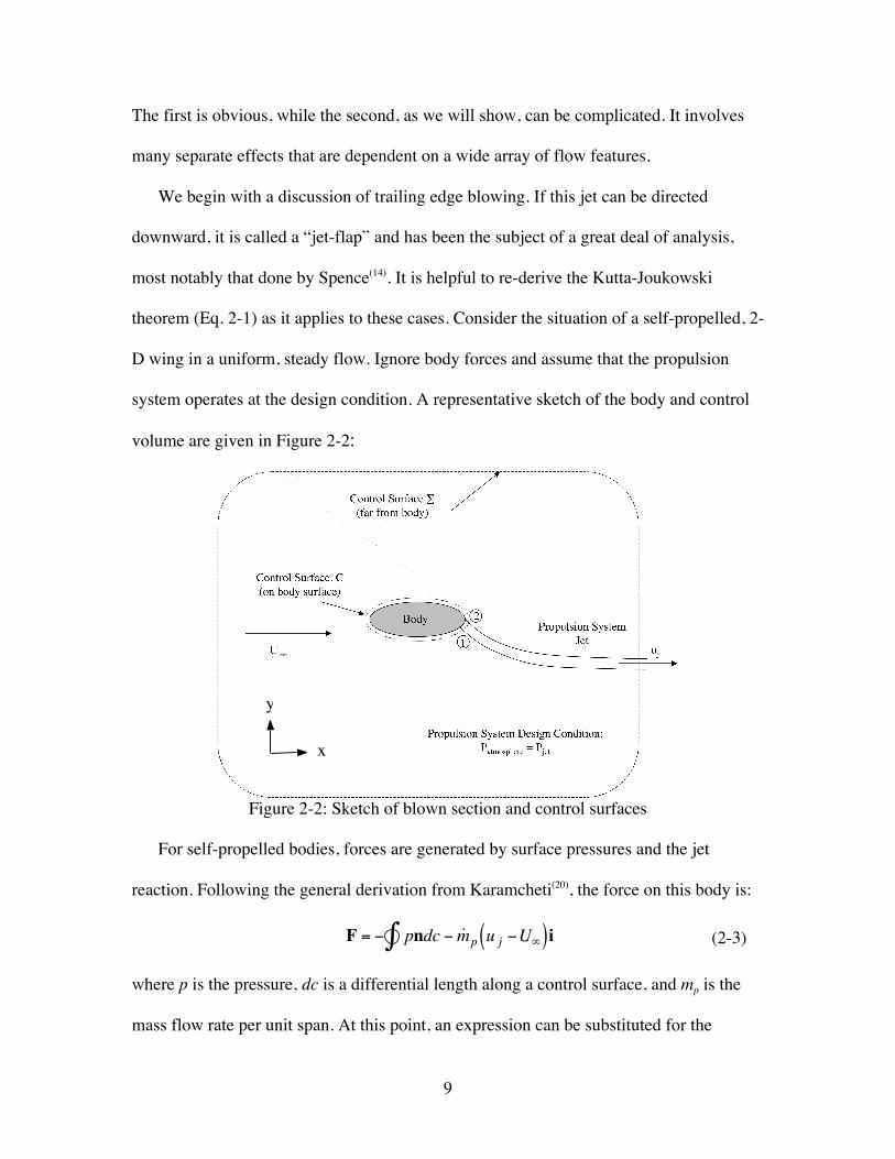
theorem (Eq. 2-1) as it applies to these cases. Consider the situation of a self-propelled, 2-
D wing in a uniform, steady flow. Ignore body forces and assume that the propulsion
system operates at the design condition. A representative sketch of the body and control
volume are given in Figure 2-2:
Figure 2-2: Sketch of blown section and control surfaces
For self-propelled bodies, forces are generated by surface pressures and the jet
reaction. Following the general derivation from Karamcheti(20), the force on this body is:
€
F = − pndc∫ − ˙ m p u j −U∞( )i (2-3)
where p is the pressure, dc is a differential length along a control surface, and mp is the
mass flow rate per unit span. At this point, an expression can be substituted for the
y
x
∞

10
pressure (Karamcheti, eq 10.62) and the behavior of this new expression examined using
the far-field control volume, Σ. Both of the control surfaces enclose the same body,
making them irreducible, reconcilable circuits. In this case, it is known that the
circulation around all such circuits has the same value. Thus, knowing the integral’s
value over the far-field control surface, the integral’s value is known over any surface
enclosing the body, including one which is right on the body surface. The force
expression is found to be (see eq. 11.92 in Karamcheti):
€
F = −ρ∞U∞ × n× q( )∫ dc − ˙ m p u j −U∞( )i (2-4)
where q is the “disturbance velocity”, i.e. the difference between the total fluid velocity
at a point and the freestream value.
Since V is the vector sum of U and q, and the condition of no flow through the body
must be satisfied over the majority of the surface, the following is assumed:
€
n×U∞dc∫ = 0 (2-5)
and,
€
n× qdc = n×Vdc∫∫ ; (2-6)
The contour integral of the cross product of the normal and velocity vectors is easy to
recognize as being the circulation around the airfoil. However, in this case, there are two
discrete portions on our contour. The majority of the surface has the typical no-flow
boundary condition, while a (typically) small portion has an outflow boundary condition
and thus has a different velocity. Referring to Figure 2-2, break the contour integral into 2
pieces:
€
F = ρ∞U∞ × n×V( )1→2∫ dc
+ ρ∞U∞ × n×V( )
2→1∫ dc
−
˙ m p u j −U∞( )i (2-7)

11
The contour integral in the first term of equation (2-7) is approximately equal to the
standard circulation value, Γ, although the presence of the jet will enforce a different
trailing edge condition and thus a modified circulation, Γmod. The second contour integral
can be evaluated since the velocity conditions at the jet surface are known. If the jet is un-
deflected, the normal and velocity vectors are parallel and this term becomes zero. If the
jet is given a deflection angle, δ, relative to the chord line this term becomes:
€
ρ∞U∞ u j t sinδ( ) (2-8)
where t is the jet thickness, i.e. approximate contour length from 2 to 1. This term
represents the contribution of the reaction force to lift. It is important to note that for
upper surface blown sections, the contour integral from 2 to 1 may also include
significant portions where the jet runs parallel with the surface. Thus, the velocity vector
is tangent to the surface and can alter the force in that fashion as well.
The total force on the body can then be written as:
€
F = ρ∞U∞Γmodk + ρ∞U∞ u j t sinδ( )k − ˙ m p u j −U∞( )i (2-9)
This is the analogy to the Kutta-Joukowski theorem for a blown airfoil. It simply states
that the jet will modify the basic circulation (super-circulation) and any surface on which
it acts, and it will produce a net thrust.
A derivation done by Siestrunck(21) comes to an analogous expression:
€
F = ρUΓk − p j + ρ jV j2( )δi (2-10)
where Γ is the total circulation of the wing-jet system, and the second term describes the
reaction lift force. (Note δ in eqn. 2-10 denotes jet width)
While the induced flow is similar to that of a simple mechanical flap, it is important
to understand where and why changes occur. In a subsonic flow, changing the trailing
12
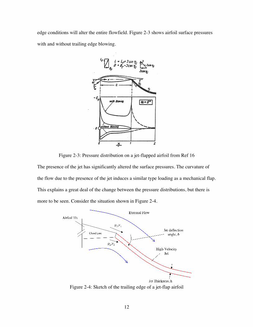
edge conditions will alter the entire flowfield. Figure 2-3 shows airfoil surface pressures
with and without trailing edge blowing.
Figure 2-3: Pressure distribution on a jet-flapped airfoil from Ref 16
The presence of the jet has significantly altered the surface pressures. The curvature of
the flow due to the presence of the jet induces a similar type loading as a mechanical flap.
This explains a great deal of the change between the pressure distributions, but there is
more to be seen. Consider the situation shown in Figure 2-4.
Figure 2-4: Sketch of the trailing edge of a jet-flap airfoil

13
The curvature of the jet sheet allows it to support a pressure difference across it, and
thus in a typical situation p2 > p1 and by Bernoulli’s equation, v1 > v2. Having the jet sheet
at the trailing edge effectively relaxes the classical Kutta condition, allowing the upper
surface and lower surface to come to different velocities at the trailing edge. Siestrunck
says, “The thin jet sheet plays the part of a regulator of the circulation as would the sharp
trailing edge of a solid flap”. Thus, the adverse pressure gradient is relieved or even
changed to a favorable one on the aft portion of the upper surface. This is another
increase in circulation. This effect could be seen even if the jet-flap angle were zero, as
will be demonstrated in later chapters.
It is worthwhile to contrast this process with that seen in “circulation-control” airfoils,
on which a significant amount of work has been done by Englar(22). These airfoils use
trailing edge blowing over a thick, rounded trailing edge. Very large increases in
circulation are seen even though the jet doesn’t play the same role as with jet-flaps or
upper surface blowing. In these cases, the circulation increase comes directly from
controlling the location of the airfoil’s stagnation points. In the present case, circulation is
gained by providing a different trailing edge condition. For this reason, higher Cµ values
are required to achieve performance than needed for a circulation control wing.
The pressure difference across the jet plays another important role. The force it
creates on the jet acts to turn the jet back into the direction of the freestream. Helmbold(23)
says that the turning force must be in equilibrium with the excess of centrifugal
acceleration in the jet. Theoretically, at infinity downstream of the airfoil, the jet becomes
parallel to the freestream regardless of its initial deflection. Since drag is zero in inviscid
14
flow, the leading edge thrust and the drag component of the turning force are equal and
opposite. Thus, in inviscid flow, it is assumed that we have full thrust recovery.
2.3 – Effects of Surface Blowing
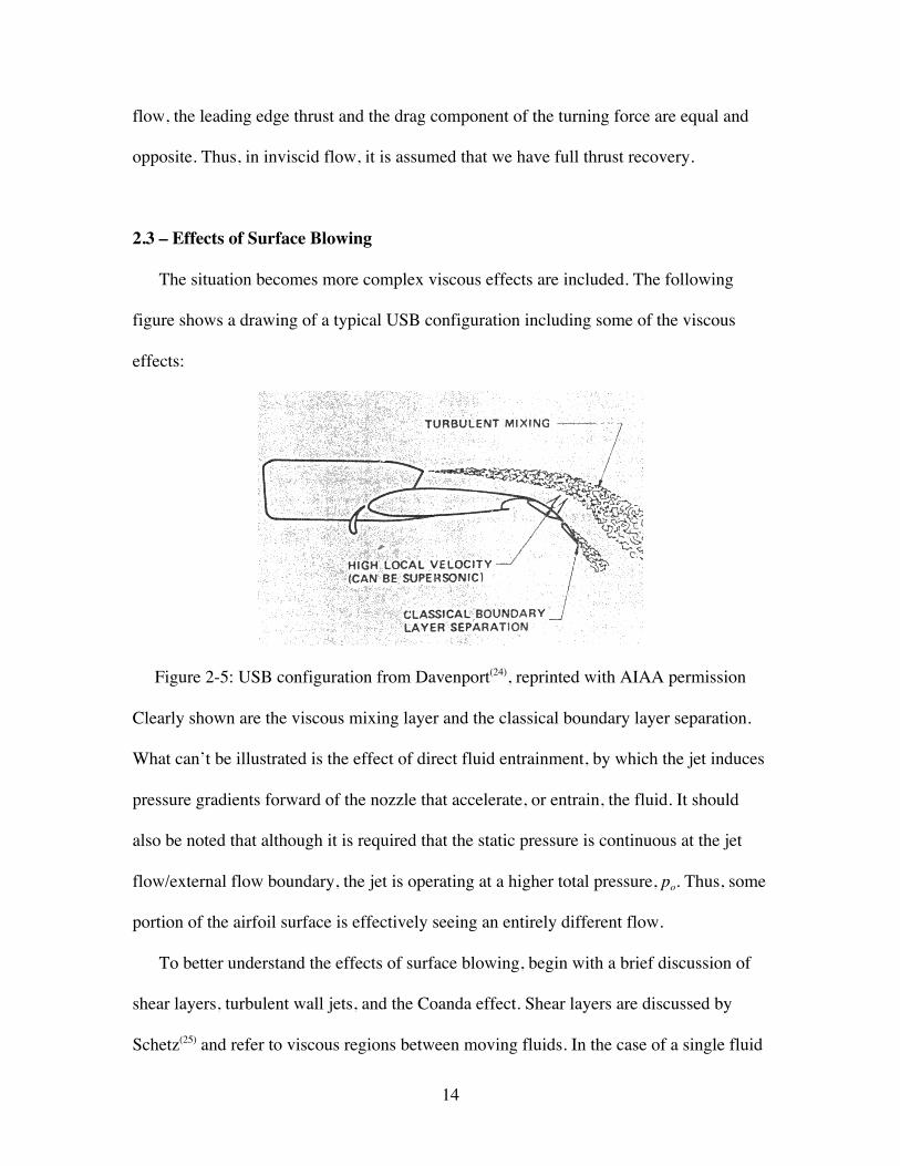
The situation becomes more complex viscous effects are included. The following
figure shows a drawing of a typical USB configuration including some of the viscous
effects:
Figure 2-5: USB configuration from Davenport(24), reprinted with AIAA permission
Clearly shown are the viscous mixing layer and the classical boundary layer separation.
What can’t be illustrated is the effect of direct fluid entrainment, by which the jet induces
pressure gradients forward of the nozzle that accelerate, or entrain, the fluid. It should
also be noted that although it is required that the static pressure is continuous at the jet
flow/external flow boundary, the jet is operating at a higher total pressure, po. Thus, some
portion of the airfoil surface is effectively seeing an entirely different flow.
To better understand the effects of surface blowing, begin with a brief discussion of
shear layers, turbulent wall jets, and the Coanda effect. Shear layers are discussed by
Schetz(25) and refer to viscous regions between moving fluids. In the case of a single fluid
15
with regions moving at different velocities, a layer of fluid is present between the flows
in which the velocity profile transitions smoothly. Similar to a boundary layer, this region
grows as momentum is diffused.
Turbulent wall jets have been studied for quite some time due to their many practical
applications. Of particular interest here are turbulent wall jets flowing over convex
surfaces. Launder and Rodi(26) provide a very good description of the phenomena
involved. Directly related to this subject is the Coanda effect, which is the remarkable
ability of a wall jet to remain attached to the adjacent curved surface even when the
surface subtends a large angle. The turbulent wall jet basically consists of an inner region
where the velocity behaves like a turbulent boundary layer, and a much larger outer
region that is similar to a shear layer.
According to Launder and Rodi, the Coanda effect is caused by momentum transfer
between the inner and outer regions. Essentially, the convex streamlines intensify
turbulent mixing in the outer region and reduce it in the inner region. This increased outer
layer mixing is a cause for the increased rate of jet growth over a curved surface as
compared to a planar one. The process of “selective amplification” of turbulent mixing
increases the importance of turbulent diffusion in the jet.
Consider now the case where a jet engine exhausts tangentially at some point on the
upper surface, instead of at the trailing edge. (The issue of aft flaps will be discussed
later) As the relatively thick jet proceeds over the curved airfoil, it behaves similarly to a
wall jet over a curved surface, but we have the additional complication of a non-uniform
external flow. The wall jet will induce lower pressures over the wetted surface. It will
also experience viscous losses due to increased mixing as it turns across the surface and
16
due to usual boundary layer effects. Thus, there is a reduction in the momentum flux
(thrust) exiting the trailing edge.
In addition, there are entrainment effects. In properly designed cases these effects can
become quite large. This is the idea behind thrust augmenters(27), where entrainment
effects effectively replace an actuator disk as the source of generating a pressure
differential. In the present case, the effects are secondary and have not been studied
significantly. The viscous interaction between the jet and the external flow can relieve
adverse pressure gradients upstream of the nozzle exit. This can provide a significant
increase in airfoil circulation.
Thus, basic viscous interactions can greatly complicate the problem. Although the
momentum flux leaving the trailing edge is less than would exist if the jet were located at
the trailing edge, a significant increase in circulation can be gained by surface blowing.
However, one must also take into account the losses that these viscous processes
introduce. An outline for thrust/drag bookkeeping is given in the next chapter.
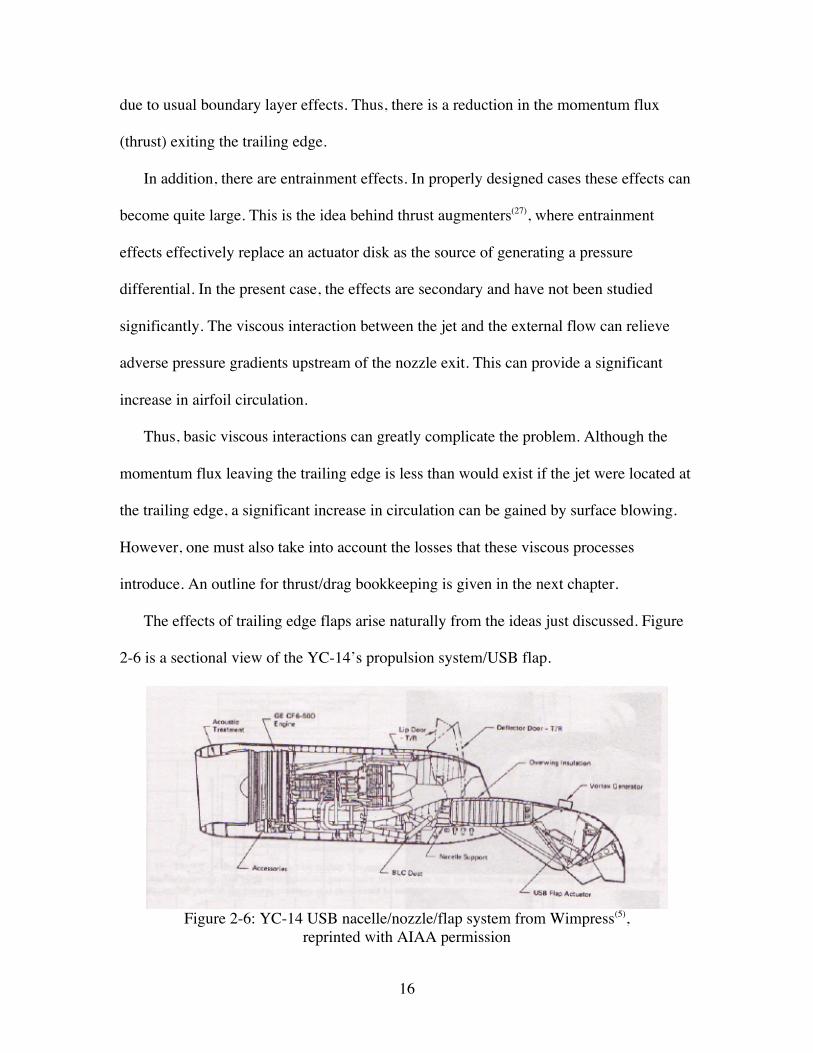
The effects of trailing edge flaps arise naturally from the ideas just discussed. Figure
2-6 is a sectional view of the YC-14’s propulsion system/USB flap.
Figure 2-6: YC-14 USB nacelle/nozzle/flap system from Wimpress(5),reprinted with AIAA permission

17
Notice that the elements of the flap system move and orient themselves in such a way as
to provide a continuous, curved surface for the jet. The primary parameters are the final
trailing edge angle and the curvature of the flap surface. Contrast this design to the multi-
element systems discussed in Reference 15 where element gap and overlap are the
primary parameters. The large curvatures of deflected flaps follow the same rules as
described above, however the viscous processes become more pronounced with flap
deflection.
As the curvature becomes large, the jet is turned through a larger angle. The viscous
shear/mixing layer grows large and can eventually breakdown the Coanda effect and
cause the jet to separate from the surface. The large curvatures also lead to lower surface
pressures on the flap. This provides the characteristic increases in lift force, but also
provides a drag force as the surface normal vector rotates away from vertical. Some of
this drag force is never realized as the leading edge suction effect increases with
circulation, but it is clear that USB flaps can produce large amounts of drag.
2.4 – Breakdown of Forces
Consider the sketch shown in Figure 2-7 of an idealized USB configuration. No
account is made for a propulsion system inlet.
18
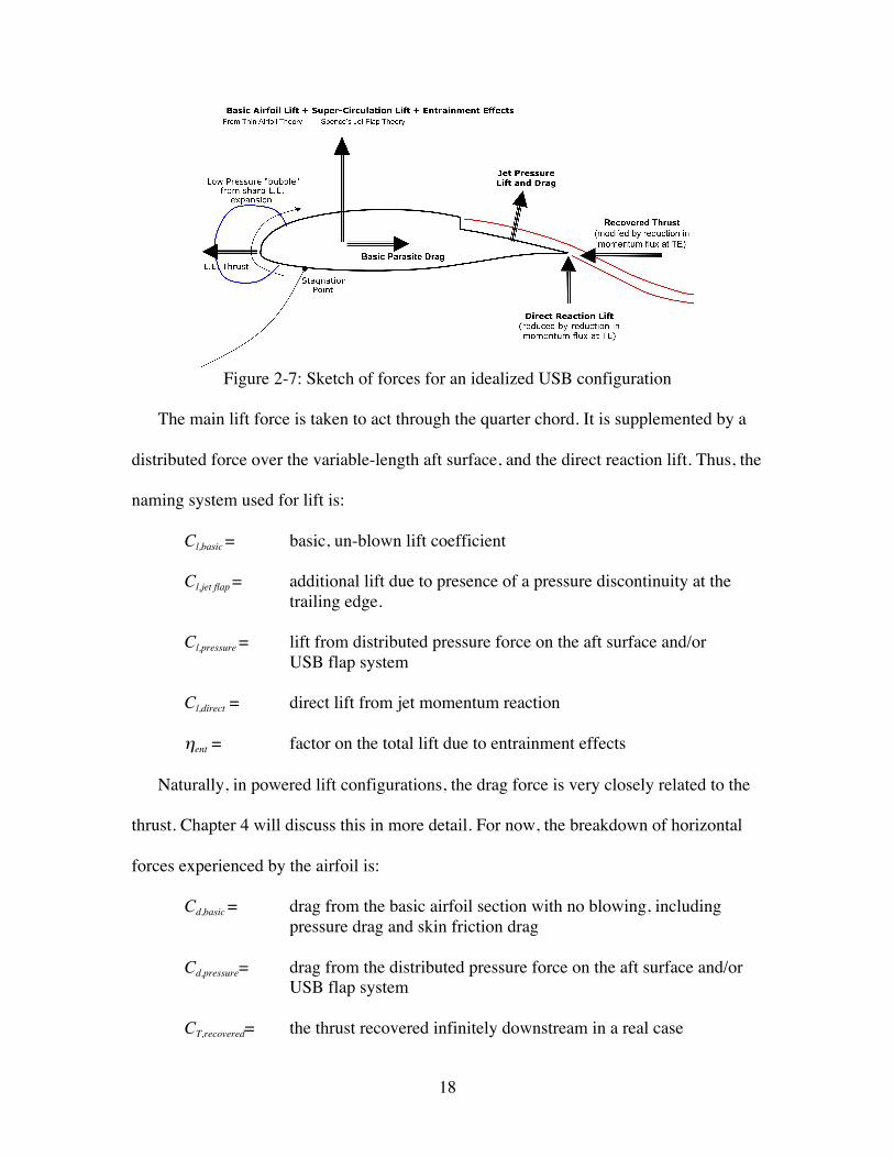
Figure 2-7: Sketch of forces for an idealized USB configuration
The main lift force is taken to act through the quarter chord. It is supplemented by a
distributed force over the variable-length aft surface, and the direct reaction lift. Thus, the
naming system used for lift is:
Cl,basic = basic, un-blown lift coefficient
Cl,jet flap = additional lift due to presence of a pressure discontinuity at thetrailing edge.
Cl,pressure = lift from distributed pressure force on the aft surface and/orUSB flap system
Cl,direct = direct lift from jet momentum reaction
ηent = factor on the total lift due to entrainment effects
Naturally, in powered lift configurations, the drag force is very closely related to the
thrust. Chapter 4 will discuss this in more detail. For now, the breakdown of horizontal
forces experienced by the airfoil is:
Cd,basic = drag from the basic airfoil section with no blowing, includingpressure drag and skin friction drag
Cd,pressure= drag from the distributed pressure force on the aft surface and/orUSB flap system
CT,recovered= the thrust recovered infinitely downstream in a real case
19
CT,LE = the suction force at the leading edge
Once the lift and drag forces are understood, the pitching moment for the USB
section becomes much clearer. It has been well documented that upper surface blowing
causes large, nose-down pitching moments. Looking at Figure 2-7, it is easy to see why.
Any airfoil modification that produces large chord loadings near the trailing edge will
have large nose-down pitching moments. An example of this is adding “aft-camber” to an
airfoil. Upper surface blowing does significantly modify the aft chord loading, and it
experiences the reaction moment from the jet leaving the trailing edge. The breakdown
for the pitching moment is very similar to that of the lift:
Cm,basic = basic moment coefficient
Cm,jet flap = additional moment due to presence of pressure discontinuity at thetrailing edge.
Cm,pressure = moment from distributed pressure force on the aft surface and/orUSB flap system
Cm,direct = direct moment from jet momentum reaction at the TE
2.5 – Adverse Effects
The purpose of this section is to describe the processes that occur in a USB design
that can decrease the performance. A large amount of experimental work has been done
to find factors that contribute to these processes and what can be done to minimize them.
The primary concern relates to the jet’s ability to turn efficiently over the flap. Also of
concern is the behavior of the leading edge when the airfoil is at high values of super-
circulation. As described by Phelps(28), the low speed performance appears to be mainly

20
dependent upon the jet turning angle and turning efficiency and on adequate leading edge
treatment to prevent premature flow separation.
When referring to a thick jet’s ability to follow a curved surface, two important
parameters must be defined clearly. First, define the turning angle, δ, as the angle through
which the exhaust jet actually turns. Second, define the turning efficiency, ηturn, as the
measure of how much of the static thrust is achieved at a given turning angle. In other
words, given a certain jet deflection, how much of the static axial thrust is successfully
turned through the angle?
The turning angle is essentially a reflection of the curvature achieved in the
mixing/shear layer. A great deal of mixing means that the jet boundary is growing thicker
and the curvature is reduced. This means that the jet will not have turned through the
desired trailing edge angle. A study from the NADC(29) contains a great deal of collected
and summarized turning data. The turning angle is primarily affected by:
1. The exhaust flow angle relative to the surface (this is referred to as the “kick-down” angle). A high nozzle kick-down angle will force the exhaust jet to bethinner.
2. The ratio of jet thickness to turning radius. A thin jet will turn much moreefficiently than a thick jet, making low values of this ratio desirable.
3. Nozzle design. This is a broad category that includes both the internal designand external design
4. Boundary layer condition over the turning surface
Clearly, the design of the nozzle to achieve a thinner jet with minimal losses is crucial for
upper surface blowing.
The turning efficiency is closely tied to the turning angle. Essentially, the jet begins
losing total pressure due to the mixing and turning process. Portions of the jet’s energy
are being absorbed by viscous processes in the boundary layer and in the mixing/shear
layer. As shown in the experimental data of Ref 28, turning efficiencies can approach 100

21
percent for small flap deflections. However, for large flap deflections, the turning
efficiency can drop to about 80 percent. This is still a favorable efficiency compared to
some other powered lift designs such as externally blown flaps(30).
The other concern noted above is that of leading edge flow separation. Referring
again to Figure 2-7, note that the stagnation point has been shifted aft on the lower
surface due to the high values of circulation. This induces the rapid leading edge
expansion shown. However, if this expansion becomes too severe, the flow may separate
at the leading edge. The correction used in all practical designs has been to incorporate
leading edge flaps or slats to soften this expansion and permit higher values of
circulation. This does slightly diminish the lift coefficient at a given configuration, but
permits a higher maximum lift coefficient. Another suggested solution by Englar(22) is to
incorporate leading edge tangential blowing (boundary layer control). This would prevent
separation and actually augment the pressure distribution.
2.6 – Three-Dimensional Behavior
While the analytical methods developed in this work are primarily for two
dimensions, it is useful to discuss the three-dimensional behavior of USB configurations.
As expected, the 3-D case cannot perform as well as the 2-D case. This is partially due to
the fact that nearly all USB designs (and certainly all those built to this point) can only
blow over limited portions of the wingspan. Nozzles designed to spread the exhaust flow
laterally are desirable, but this spreading can incur losses if not done properly. For this
discussion, only partial-span blowing designs are considered.
22
As described by Phelps(28) and demonstrated in other configuration data, upper surface
blowing exhibits a “localized” flow behavior. This means that there is very little lateral
spreading of the jet. Contrast this with the behavior of externally blown flaps where the
jet impinges on the lower surface of the flap and spreads spanwise. In a USB
configuration, the jet influence is confined to a localized region by the formation of
vortices on the edges of the jet sheet.
Perhaps the most significant decrease in performance comes from induced drag. As
described by Mason in Reference 15, the induced drag is a function of the spanloading.
The localized nature of USB leads to relatively sharp changes in the spanloading, which
in turn can lead to higher values for the induced drag. While this is offset by the
enormous gains in lift performance, it can still be an issue.
The full three-dimensional problem has been studied using modified panel methods
(Narain(31)), zonal methods (Roberts(12)), and wing-wake vortex lattice methods
(Mendenhall(13)). However, these methods can be costly to set up for a given
configuration. For example, the panel methods must be determined for the configuration
including special paneling schemes for the nacelle and flap surface. In addition, an
iterative scheme must be used to determine the jet position given the specific propulsion
conditions. The zonal method, while it has the potential to be a very accurate method, is
very costly to set up due to the fact that a very complex grid must be developed for even
a basic problem. The vortex lattice method was more successful, but still was hard to use
and often significantly over-predicted the wing lift performance.

23
Chapter 3: Thrust/Drag Bookkeeping for USB Designs
The closely coupled interactions between the aerodynamics and propulsion in
powered-lift configurations can be a major problem area for a design. The idea of
integrating the propulsion system into the wing has been around since the advent of jet
propulsion. Creating efficient integrated designs is the essence of multidisciplinary
design optimization (MDO). The design of efficient wing/nacelle combinations is the first
step toward fully integrated propulsion/aerodynamic design. Powered-lift aircraft will
never achieve their full potential without an integrated design approach.
There are two main purposes of this chapter. The first is to present the different areas
where losses should be accounted for. This will draw on the discussion of Chapter 2
regarding the flow physics involved. A possible “bookkeeping” system for powered-lift is
also suggested. The second purpose is an attempt to establish simple empirical methods
for estimating these losses. While no one way is absolutely correct, we can reduce
confusion by addressing these areas and being consistent.
24
3.1 - Losses and Bookkeeping
Following Rooney(32), for a steady flight state a balance exists between the
installed propulsive force and the drag:
€
FIPF = D (3-1)
This installed propulsive force includes throttle dependent forces. In the case of USB, this
is a little more vague. It is desirable to eliminate as much throttle dependence as possible
from the drag polars, however, unlike conventional configurations the lift is primarily
throttle dependent. The following losses dominate USB aero/propulsion integration:
1. Nozzle losses - These losses come from the need to get a high aspect ratio “thin”jet from an annular engine flow.
2. Scrubbing losses - “Scrubbing” refers to the action of the turbulent jet on anadjacent surface. This is typically the upper wing/flap surface but can include thefuselage.
3. Mixing/flow turning losses - These losses are possibly the hardest to studyanalytically. This is because they are essentially losses due to turbulentmomentum transfer with both the external free-stream flow and the boundarylayer.
4. Thrust Recovery - Thrust recovery refers to the ability of a deflected jet to returnparallel to the free-stream velocity.
A basic look at these processes shows that they are all throttle dependent. However,
some of them may contribute to the lift and pitching moment. The primary example is the
process of scrubbing, which gives an additional form drag, while providing significant
contributions to lift and pitching moment. This problem was identified by Bowers(33) for
the Quiet Short-haul Research Aircraft (QSRA). Based on this argument, it is suggested
that any mechanism that contributes significantly to both lift and drag will be included in
the polar even though it may be strongly throttle dependent.
25
Thus, the installed propulsive force would consist of:
€
FIPF =Tref + ΔTnozzle + ΔTturning + ΔTdownstreamrecovery
(3-2)
where Tref is the thrust including any cruise nozzle penalties, ΔTnozzle represents any losses
due to changing the nozzle shape (such as increasing aspect ratio for high-lift purposes),
ΔTturning represents losses associated with flow mixing, and the last term represents any
losses due to incomplete thrust recovery. These are throttle-dependent, but they do not
contribute to lift/pitching moment.
The drag force is:
€
D = Dbase + ΔDscrubbing + Dinduced (3-3)
where Dbase consists of the normal sources of aerodynamic drag, ΔDscrubbing is the
additional friction/form drag due to scrubbing, and Dinduced represents the induced drag
from circulation shed into the wake. While the scrubbing term is clearly throttle-
dependent, it is also a source of lift/pitching moment. Note that “ram” drag is not
accounted for in this analysis.
This form of bookkeeping is somewhat different than some seen in other papers,
where the drag polars reflect the whole “Thrust+Drag” term. There are advantages to
viewing the polars this way. First, for a given throttle setting, it shows where a limit
exists for level flight (when thrust plus drag becomes positive). Second, since one is
basically looking at “excess thrust” or “excess drag”, the flight path angle is easy to
determine. Thus, for a given climb angle/approach angle and a given power setting, the
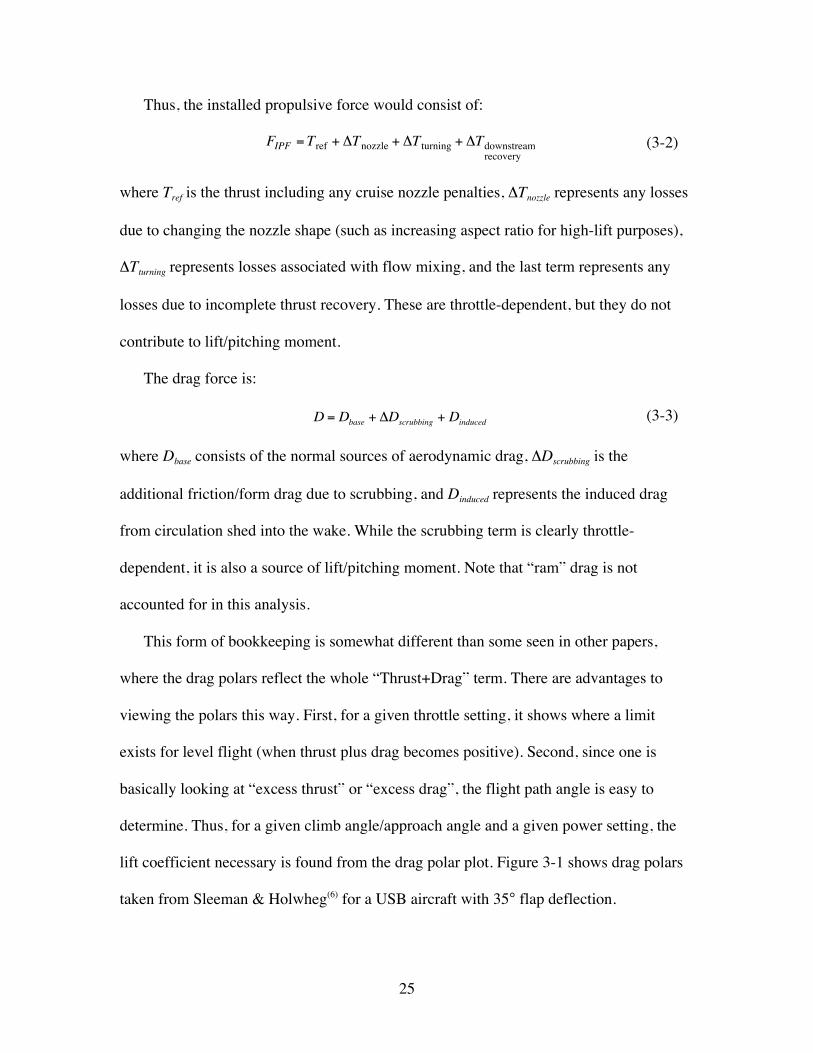
lift coefficient necessary is found from the drag polar plot. Figure 3-1 shows drag polars
taken from Sleeman & Holwheg(6) for a USB aircraft with 35° flap deflection.
26
0.0
1.0
2.0
3.0
4.0
5.0
6.0
7.0
8.0
-2.5 -2.0 -1.5 -1.0 -0.5 0.0 0.5 1.0 1.5
CD-CT
CLData, CT=0.9Data, CT=2.0Data, CT=3.0
Figure 3-1: Drag Polars for a four-engine USB configuration at 35 deg flaps
However, the plots can be misleading. They give no impression of how the drag itself
is changing with increasing power setting. In a similar fashion, the thrust losses are
implicit in the “thrust+drag” term. The aerodynamic drag can be obtained from these
plots only when the thrust and associated thrust losses are known so they can be removed.
In addition, most design codes accept input of the aerodynamic drag only, so the thrust-
plus-drag values would have to be separated manually before they would be usable. For
these reasons, we will keep the two quantities separated as much as possible using the
procedures presented above. When presenting comparisons, the familiar thrust-plus-drag
format will be used, but only after the individual calculated quantities are combined.
Thus, the individual contributions are made clear.
3.2 - Estimating Losses
This section deals with finding ways to estimate the losses discussed above for a
given configuration and propulsion state. These estimates draw heavily on published
27
experimental data, from which empirical relations can be developed. If data for a specific
configuration is available, it will supercede these relations.
First, look at losses developed by the nozzle. Depending on the nozzle design, the
magnitude of these losses can vary significantly. Jet shape is crucial to USB performance,
but nozzle exit area must correspond to the engine flow condition. Previous designs have
been forced to incorporate nozzle geometry-changing schemes to satisfy different
conditions. These losses are counted against the propulsion system. In the case of the YC-
14, nozzle effects were treated as losses to allow the “reference” thrust of the engine to be
that of the engine by itself. Some aircraft design software has internal routines for
estimating nozzle losses, but these losses will not be estimated as a part of this work.
The next category is scrubbing losses. These include the skin friction and induced
surface pressures. As mentioned before, since these tie most closely to the aerodynamic
performance, these effects will be accounted for by aerodynamics and will not affect
propulsion. The skin friction will be discussed more thoroughly in Chapter 4, as will a
method for predicting the induced surface pressures. There can be significant
contributions to the lift, drag, and pitching moment from these local pressures.
We can now discuss the turning losses, which come from the reduction of curvature
the flow experiences due to mixing. Completely understanding the process causing these
losses could require extensive numerical analysis. Fortunately, since these losses are the
main factor in how well a jet turns over a Coanda flap, there is a lot of test data upon
which to base an empirical approximation(29),(34),(35). The turning angle was defined
previously as the actual angle through which the exhaust jet is turned compared to the
28
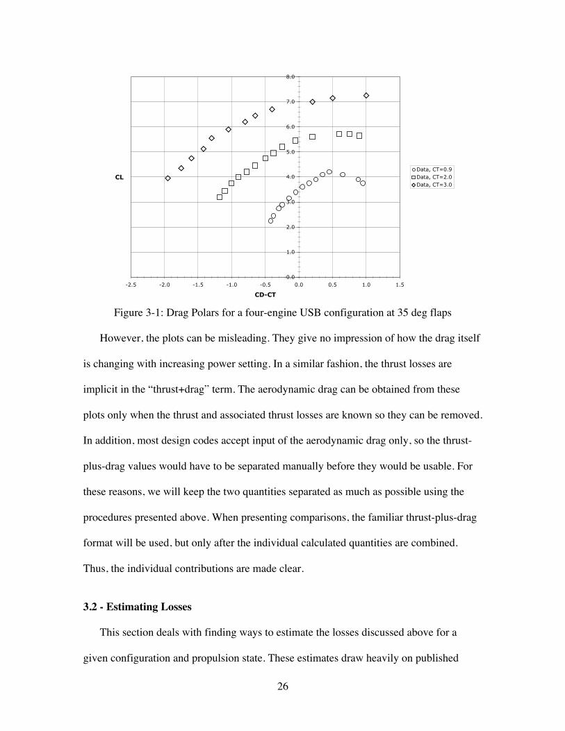
flap angle. Figure 3-2 demonstrates the nozzle kick-down angle, θkd, which is a driving
factor in turning angle efficiency.
Figure 3-2: Sketch of nozzle exhaust flow angles
Based on results presented in Reference 29, the achievable flow turning angle is a strong
function of the kick-down angle and the ratio of jet thickness to flap curvature, h/R. For
typical height-to-radius ratios of 0.3 or less, the flow turning angle can be approximated
using:
€
δ j = δ f 1− exp −10+ 29.3(h /R( ) − (0.567(h /R)(θ kd (deg)( )[ ] (3-4)
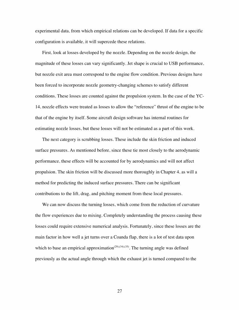
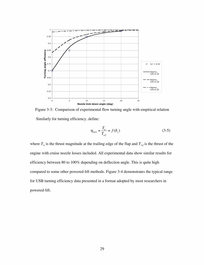
Clearly, better jet turning comes from having a thinner jet. Figure 3-3 shows
experimental data for h/R=0.3 along with the empirical relation of equation 3-4. It should
be noted that cases having larger h/R ratios would require more empirical development,
and equation 3-4 should not be used.
29
0.5
0.55
0.6
0.65
0.7
0.75
0.8
0.85
0.9
0.95
1
0 5 10 15 20 25
Nozzle kick-down angle (deg)
Tu
rnin
g a
ng
le e
ffic
ien
cy
h/r = 0.30
Approx,h/R=0.30
Approx,h/R=0.28
Approx,h/R=0.20
Figure 3-3: Comparison of experimental flow turning angle with empirical relation
Similarly for turning efficiency, define:
€
ηturn =TteTref
= f (δ j ) (3-5)
where Tte is the thrust magnitude at the trailing edge of the flap and Tref is the thrust of the
engine with cruise nozzle losses included. All experimental data show similar results for
efficiency between 80 to 100% depending on deflection angle. This is quite high
compared to some other powered-lift methods. Figure 3-4 demonstrates the typical range
for USB turning efficiency data presented in a format adopted by most researchers in
powered-lift.
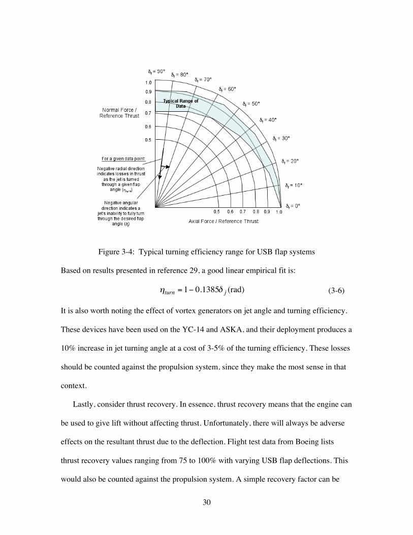
30
Figure 3-4: Typical turning efficiency range for USB flap systems
Based on results presented in reference 29, a good linear empirical fit is:
€
ηturn = 1− 0.1385δ j (rad) (3-6)
It is also worth noting the effect of vortex generators on jet angle and turning efficiency.
These devices have been used on the YC-14 and ASKA, and their deployment produces a
10% increase in jet turning angle at a cost of 3-5% of the turning efficiency. These losses
should be counted against the propulsion system, since they make the most sense in that
context.
Lastly, consider thrust recovery. In essence, thrust recovery means that the engine can
be used to give lift without affecting thrust. Unfortunately, there will always be adverse
effects on the resultant thrust due to the deflection. Flight test data from Boeing lists
thrust recovery values ranging from 75 to 100% with varying USB flap deflections. This
would also be counted against the propulsion system. A simple recovery factor can be

31
applied to the thrust at the trailing edge. For flap deflections less than ~40 degrees, it will
be assumed that there is a full thrust recovery. For deflections greater than 40 degrees, a
recovery factor of 0.95 should be sufficient to approximate this effect. In most cases,
assuming complete thrust recovery would alter results very little.

32
Chapter 4: Development of a Two-Dimensional Analytical Method
The development of a methodology for USB calculations in two dimensions is the
heart of the current work. The need for these types of calculations was described in
Chapter 1. It was also shown that to be effective in the early design stages of an aircraft,
any methodology should be fast, robust, and cost effective. In this chapter, we will
discuss the basis for the method, explain it’s constituent pieces, and introduce correlation
factors. Chapter 5 will then present results of the method with published experimental
data.
4.1 – Basis for method / Overview
Since the goal is to provide performance calculations early in the design process, the
use of Computational Fluid Dynamics was effectively ruled out due to the amount of time
needed to obtain CFD solutions. This is especially true when a configuration may be
changing very quickly early in the design process. Thus, more basic inviscid methods
were used. Viscous effects can then be approximated through correlation factors or
empirical relations. For preliminary and conceptual design this is the general standard.
33
Based on a survey of the literature available for upper surface blowing, and powered-
lift in general (see Appendix A for an annotated bibliography), it was clear that classic
jet-flap theory was inadequate for upper surface blown configurations. However, studies
have been published by Hough(36) showing that the “jet-flap analogy” can be very useful
in predicting lift and pitching moment increments due to changes in geometry or flight
state. As confirmed by Hough, Gainer(37), and Lan(18), it is expected that jet-flap theory
under-predicts the total lift and pitching moment because it does not take into account the
interaction between the wing and the jet, nor the general viscous nature of the jet flow.
Knowing this, if the surface pressures for those areas wetted by the jet can somehow
be predicted, the total forces can be approximated much better. It was found here that
Circular Streamline Theory (CST) provided a good approximation and was very easy to
use. Its derivation will be shown later in this chapter. In addition, empirical relations
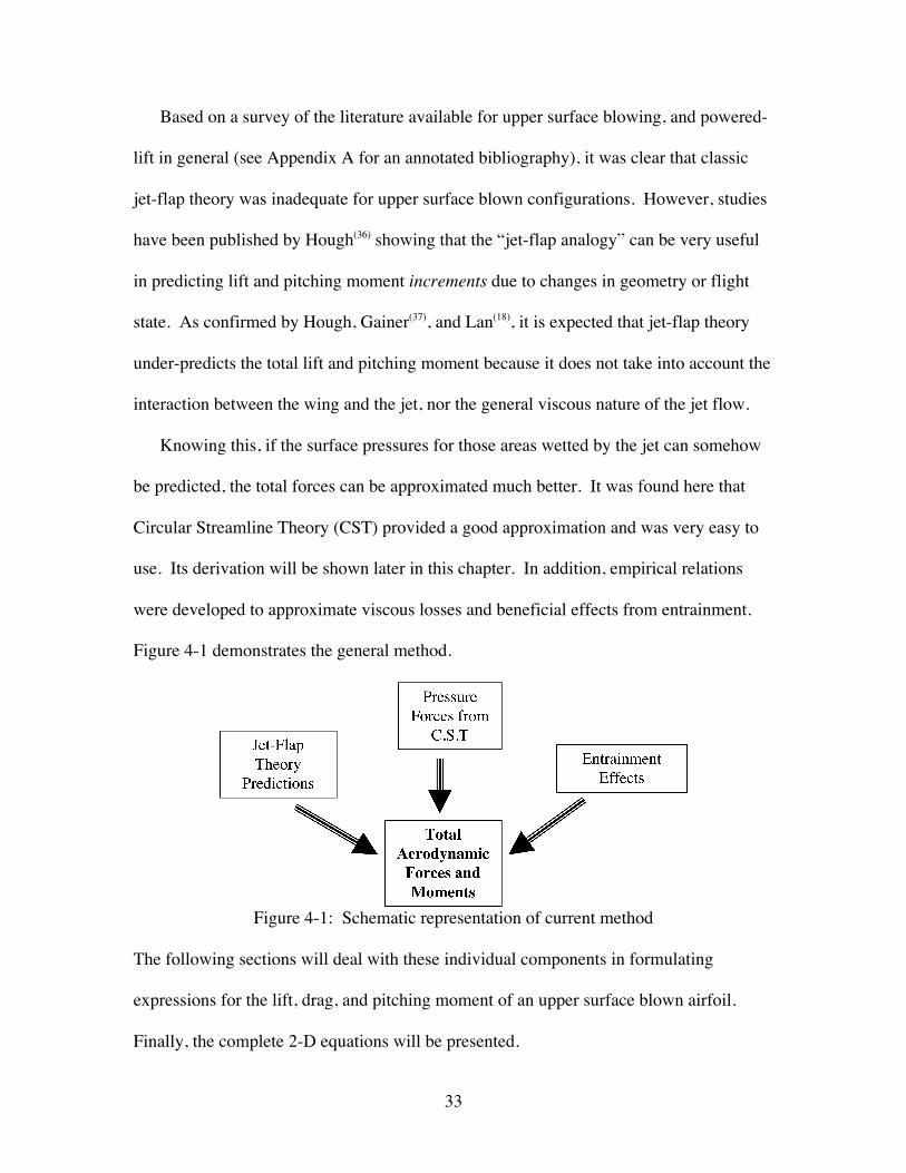
were developed to approximate viscous losses and beneficial effects from entrainment.
Figure 4-1 demonstrates the general method.
Figure 4-1: Schematic representation of current method
The following sections will deal with these individual components in formulating
expressions for the lift, drag, and pitching moment of an upper surface blown airfoil.
Finally, the complete 2-D equations will be presented.
34
4.2 – Spence’s Jet-Flap Theory
Classical Jet-Flap theory refers to the development by Spence(14),(38) in the mid 1950s.
His original work was for inviscid, incompressible flow past a thin, 2-D airfoil at
moderate incidence with a thin jet exhausting from the trailing edge. It was later
extended to include cases where the jet enters the flow tangentially along a deflected flap.
The appeal of these methods comes from their success in analyzing jet-flap wings and
from the simplicity of the method. For complete details of the analysis, the reader may
refer to Spence’s papers. A brief outline is given below.
Assume that both the main flow and jet flow are irrotational. Thus, similar to thin-
airfoil theory, a solution for a given flow can be obtained by constructing an equivalent
problem involving fundamental singularities and imposing appropriate boundary
conditions. The jet is modeled as being bounded by vortex sheets. There is no flow
across the sheets, and the tangential velocity across the sheet is continuous. The jet’s
effect on the external flow is then the same as a vortex sheet whose strength distribution
is governed by jet sheet’s curvature and momentum flux.
Assuming that the jet sheet returns to the undisturbed freestream direction, Spence
obtained an integro-differential equation for the problem. The solution was expressed
using a Fourier series, together with a function that has the correct singular behavior at
the trailing edge. Spence then formulated a 9-term interpolation to the series using a
computer for values of the momentum flux coefficient, Cj, from 0.01 to 10.
4.2.1 – Lift Coefficient
The lift coefficient is given as:
τπαππα ool ABC 422 ++= (4-1)
35
where α is the angle of attack and τ is the jet deflection angle relative to the chord line.
The coefficients Ao and Bo are the leading Fourier coefficients associated with jet
deflection and angle of attack. A curve fit based on Cµ was given as:
2/32/1
2/32/1
0041.00880.00917.0
0124.00259.02817.0
µµµ
µµµ
CCCB
CCCA
o
o
++=
++=(4-2),(4-3)
When a partial chord trailing edge flap is added, the equations must be modified
slightly. Note that jet-flap theory does not account for interactions of the jet with the flap
surface. The jet is essentially treated as coming from the deflected flap’s trailing edge,
and the flow along the surface provides the benefit of eliminating any flow separation.
The sectional lift coefficient is given by:
( ) fool DBC δπχχαππα 2sin242 ++++= (4-4)
where Bo is identical to that above. The variable, χ, is defined as:
)(sin2 1 E−=χ (4-5)
where E is the ratio of flap chord to airfoil chord. Implicit is the assumption that the jet
angle is the same as the flap deflection angle, δf.
Spence did not provide similar curve fits for Do, since it is a complicated function of
both Cµ and E. He simply presented the values graphically using families of curves for
the different values of E. Based on these graphs, a multi-variable interpolated function
was constructed for Do as part of the current work using non-linear regression analysis.
The function obtained is:
€
Do = Ao +−1.931E
14
4πCµ(−0.9621E 2 +0.5785E +0.1639)( ) (4-6)
36
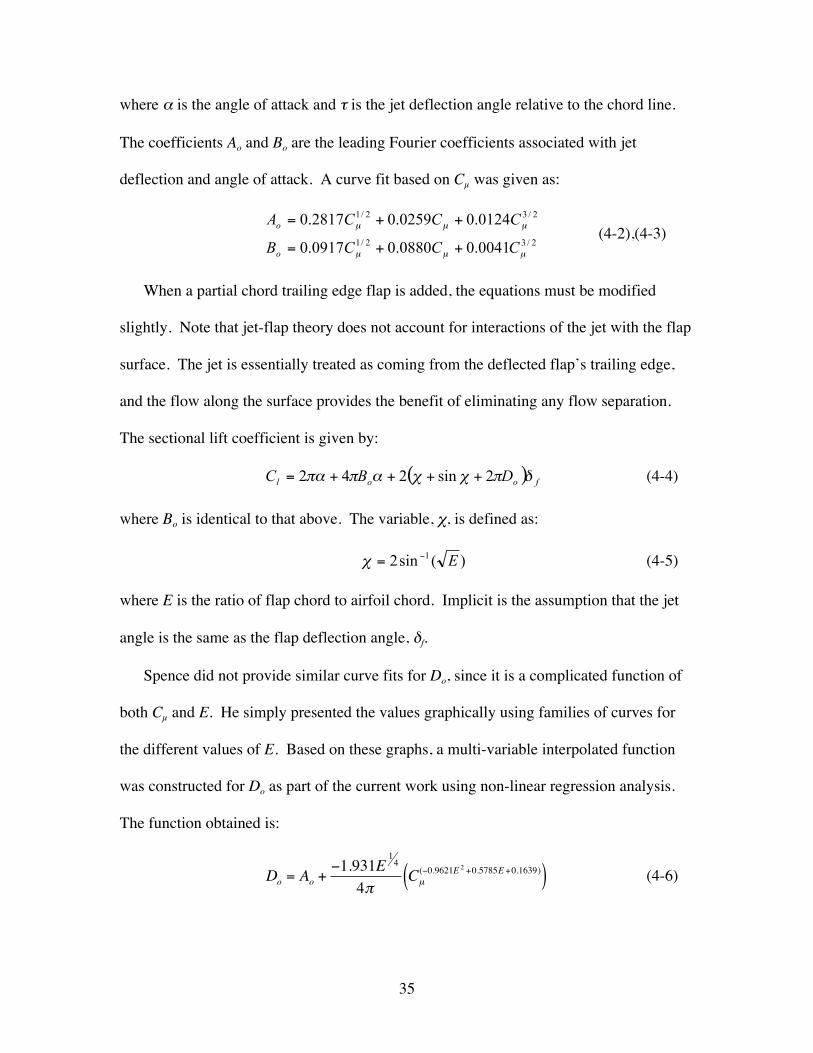
Clearly, Ao is the limit as E goes to zero, i.e., as the flap becomes small the performance
becomes more like a pure jet-flap. Figure 4-2 shows data points taken from Spence(38)
along with the interpolating function given in equation (4-6).
0
2
4
6
8
10
12
14
0 0.5 1 1.5 2 2.5 3 3.5 4 4.5 5
Blowing Coefficient, C j
dCl/dδf
E=0
E=0.02
E=0.05
E=0.1
E=0.2
E=0.3
InterpolatedFunction
Figure 4-2: Agreement of dCl/dδf using derived approximate function (4-6)
The basic jet flap theory originally developed by Spence was extended by W. H.
Davis(39) at Grumman Aerospace in 1979 to include camber effects. The study was
limited to thin airfoils with parabolic camber. Note that this extension was originally
done only for a pure jet flap. The sectional lift coefficient is given by:
γππγτπαππα oool CABC 44442 ++++= (4-7)
where γ is the airfoil camber as a percent of the chord, and τ is now referenced from the
non-zero trailing edge angle. A curve fit for Co using similar powers of Cµ is :
2/32/1 0922.04499.00600.0 µµµ CCCCo −+= (4-8)

37
As clearly shown from comparing equations (4-1) and (4-7), the camber effect is
purely additive via the last two terms of equation (4-7). This is not surprising, since this
is a linear analysis thus superposition of solutions is valid. The first of the camber terms
expresses the change in lift coefficient purely due to camber, the second (involving Co) is
dependent on the momentum coefficient. Combining the effects of a partial-chord flap
with airfoil camber, the following expression is obtained for the lift coefficient:
€
Cl = 2πα + 4πBoα + 2 χ + sinχ + 2πDo( )δ f + 4πγ 1+Co( ) (4-9)
4.2.2 – Pitching Moment Coefficient
In the case of a pure jet flap, the pitching moment is expected to be influenced by the
blowing coefficient, Cµ, through both the angle of attack, α, and the jet deflection angle,
τ. The general form of the pitching moment about the leading edge is:
€
Cm,le = −12π + Eo
α + Foτ (4-10)
where Eo and Fo are coefficients that are functions of the blowing coefficient, very similar
to the coefficients defined in the lift calculations. For the case of no blowing, the
standard thin airfoil result is recovered. Good curve fits using data from Spence are:
€
Eo = −0.3057C j1/ 2 − 0.2466C j + 0.0406C j
3 / 2
Fo = −1.5868C j1/ 2 − 0.6945C j − 0.0437C j
3 / 2(4-11),(4-12)
In the case of a trailing edge flap with a jet, the pitching moment’s angle of attack
relationship will remain the same, but the change due to the aft flap must be accounted
for. A superposition of the classical flap contribution and the additional effects of the jet
deflection leads to:
€
Cm,le = −12π + Eo
α −
12χ + sin(χ) +
14sin(2χ)
δ f +Goδ f (4-13)

38
where Go is a coefficient dependent on both Cj and flap chord.
Finding a functional relation for Go was difficult due to the limited data provided by
Spence. In addition, since he only provided pitching moment data up to a blowing
coefficient of 5, one cannot use curve fits that significantly deviate for high blowing
coefficients (such as high-order polynomials). It was originally hoped that a single
functional relationship could be established for any flap chord, but that proved difficult.
In addition, it would be largely unnecessary since the overwhelming majority of designs
use flap chord ratios of 0.20 to 0.35. Thus, the easiest approach for any practical design
was to simply establish a good fit for Go based on Spence’s data at a flap chord of 0.30:
€
Go = −0.3318Cµ1/ 2 −1.0332Cµ + 0.0842Cµ
3 / 2 (4-14)
At this point, the moment can be transferred to the quarter chord location as:
€
Cm,0.25c =14Cl + Cm,le (4-15)
This completes the current use of the jet-flap theory. Since it is based on 2-D thin airfoil
theory (note that all the previous equations reduce to the classic formulas when there is
no blowing) no drag force can be predicted from the theory. Drag will be discussed in
detail later in this chapter.
4.3 – Circular Streamline Theory
Having a well-documented, analytical method for the jet-flap is a key step for
powered-lift designs. However, as mentioned previously, the basis of classical jet-flap
analysis is inviscid, thin-airfoil theory. The flow of the jet over the surface is not
accounted for and this does introduce discrepancies into the analysis. A method should
be devised to approximate the surface pressures induced on the curved surface wetted by
39
the jet. The most precise way of doing this would include a complete analysis of a wall-
jet flowing over a convex surface in the presence of a non-uniform external flow field.
Such an analysis is not possible analytically, though some approximate work was done by
Roberts(39).
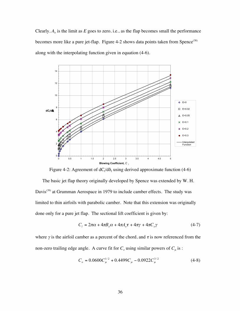
Since only an approximation is needed, a simpler approach is proposed. We theorize
that the nearly circular attached flow streamlines produced by coanda effect can be
represented by potential flow, since that flowfield has circular streamlines and satisfies
the boundary condition on the circular surface. A typical wall-jet velocity profile is
shown in Figure 4-3.
Figure 4-3: Example of a wall jet velocity profile
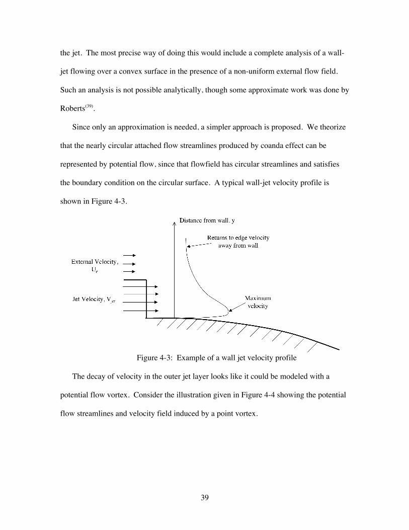
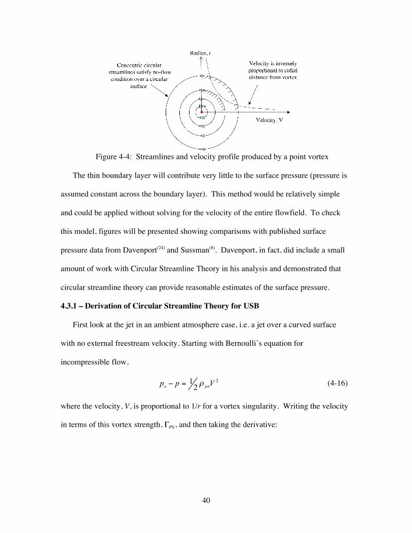
The decay of velocity in the outer jet layer looks like it could be modeled with a
potential flow vortex. Consider the illustration given in Figure 4-4 showing the potential
flow streamlines and velocity field induced by a point vortex.
40
Figure 4-4: Streamlines and velocity profile produced by a point vortex
The thin boundary layer will contribute very little to the surface pressure (pressure is
assumed constant across the boundary layer). This method would be relatively simple
and could be applied without solving for the velocity of the entire flowfield. To check
this model, figures will be presented showing comparisons with published surface
pressure data from Davenport(24) and Sussman(8). Davenport, in fact, did include a small
amount of work with Circular Streamline Theory in his analysis and demonstrated that
circular streamline theory can provide reasonable estimates of the surface pressure.
4.3.1 – Derivation of Circular Streamline Theory for USB
First look at the jet in an ambient atmosphere case, i.e. a jet over a curved surface
with no external freestream velocity. Starting with Bernoulli’s equation for
incompressible flow,
2
21 Vpp jeto ρ=− (4-16)
where the velocity, V, is proportional to 1/r for a vortex singularity. Writing the velocity
in terms of this vortex strength, ΓPV, and then taking the derivative:

41
€
po − p = 12ρ jetΓPV2
4π 2r 2
dpdr
= ρ jetΓPV2
4π 2r 3
(4-17),(4-18)
This ODE is integrable, so integrate p from pwall to p, and r from R to R+t where t is the
thickness of the jet. This gives:
€
p− pwall =−ρ jetΓPV
2
2(4π 2)1
(R + t)2−1R2
(4-19)
Since p at the edge of the jet is equal to the local static pressure, which is p∞, the LHS can
be re-arranged to give the familiar quantity, Δp. The important remaining part is
determining the appropriate value of the vortex strength, ΓPV. This quantity will be
determined by satisfying the maximum jet velocity (which is known) at a given radius.
Refer to this arbitrary location as the “reference” radius, Rref. Again, writing the vortex
strength in terms of Vexit and r gives:
−
+=Δ 22
22 1)(
12 RtR
VRp exitrefjetρ
(4-20)
and for Cp based on the jet dynamic pressure this leads to:
−
+= 22
2 1)(
1RtR
RC refp (4-21)
The approximation is clearly dependent on the radius used to find ΓPV. It is useful to
examine this development compared to experimental surface pressures of wall jets
flowing over curved surfaces. Figure 4-5 shows an experimental setup used by
Davenport(24) to measure the surface pressures induced over a curved USB flap.
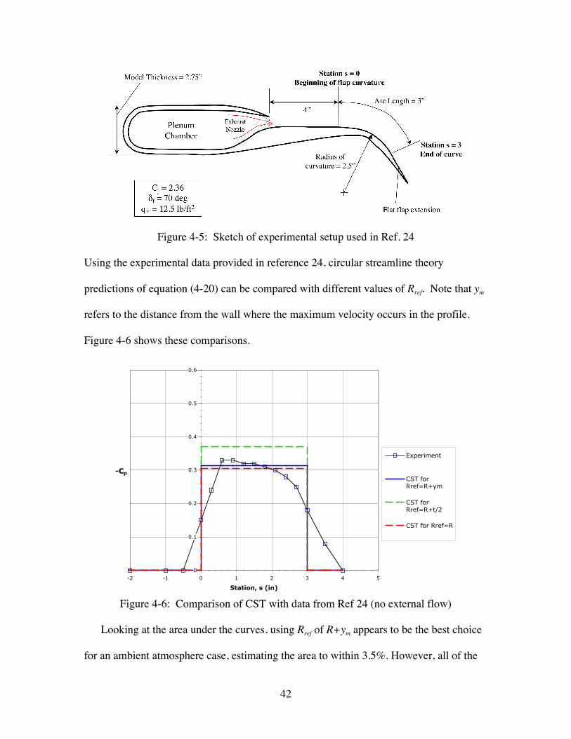
42
Figure 4-5: Sketch of experimental setup used in Ref. 24
Using the experimental data provided in reference 24, circular streamline theory
predictions of equation (4-20) can be compared with different values of Rref. Note that ym
refers to the distance from the wall where the maximum velocity occurs in the profile.
Figure 4-6 shows these comparisons.
0
0.1
0.2
0.3
0.4
0.5
0.6
-2 -1 0 1 2 3 4 5
Station, s (in)
-Cp
Experiment
CST forRref=R+ym
CST forRref=R+t/2
CST for Rref=R
Figure 4-6: Comparison of CST with data from Ref 24 (no external flow)
Looking at the area under the curves, using Rref of R+ym appears to be the best choice
for an ambient atmosphere case, estimating the area to within 3.5%. However, all of the
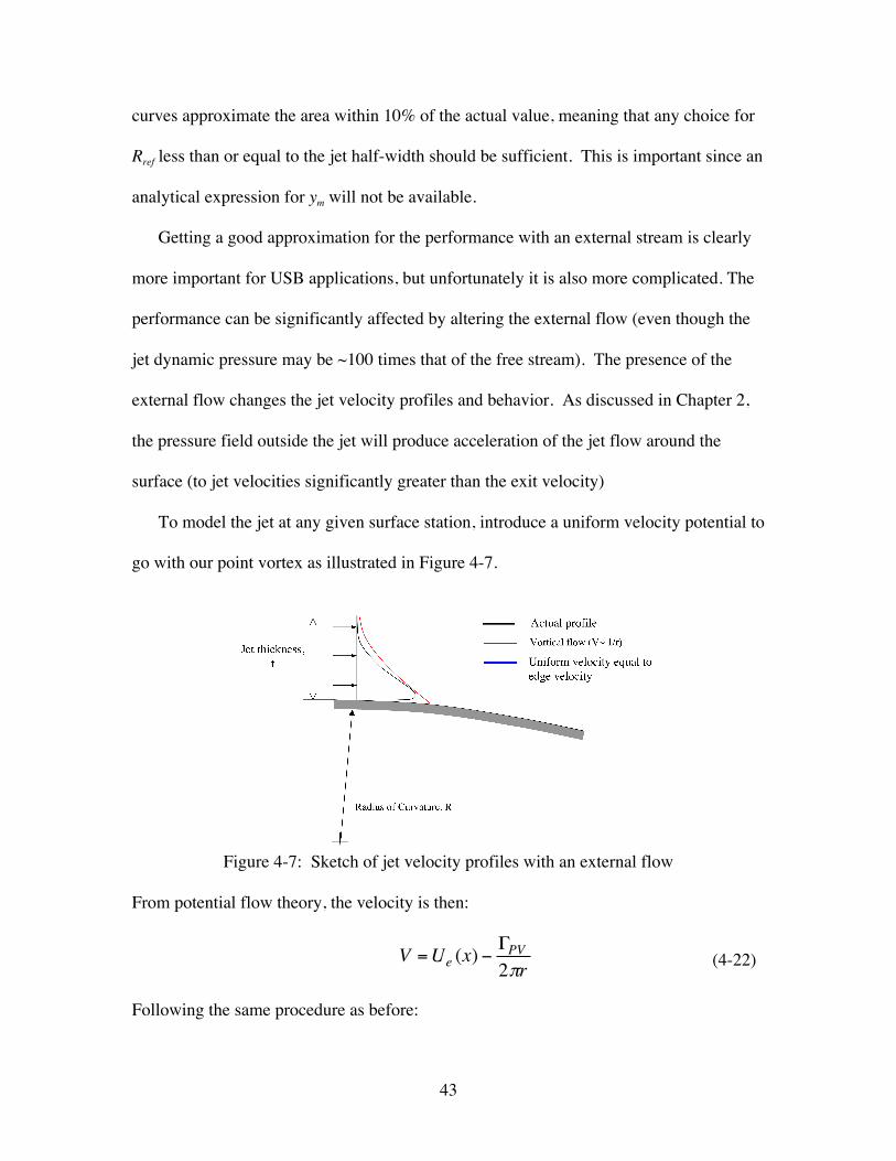
43
curves approximate the area within 10% of the actual value, meaning that any choice for
Rref less than or equal to the jet half-width should be sufficient. This is important since an
analytical expression for ym will not be available.
Getting a good approximation for the performance with an external stream is clearly
more important for USB applications, but unfortunately it is also more complicated. The
performance can be significantly affected by altering the external flow (even though the
jet dynamic pressure may be ~100 times that of the free stream). The presence of the
external flow changes the jet velocity profiles and behavior. As discussed in Chapter 2,
the pressure field outside the jet will produce acceleration of the jet flow around the
surface (to jet velocities significantly greater than the exit velocity)
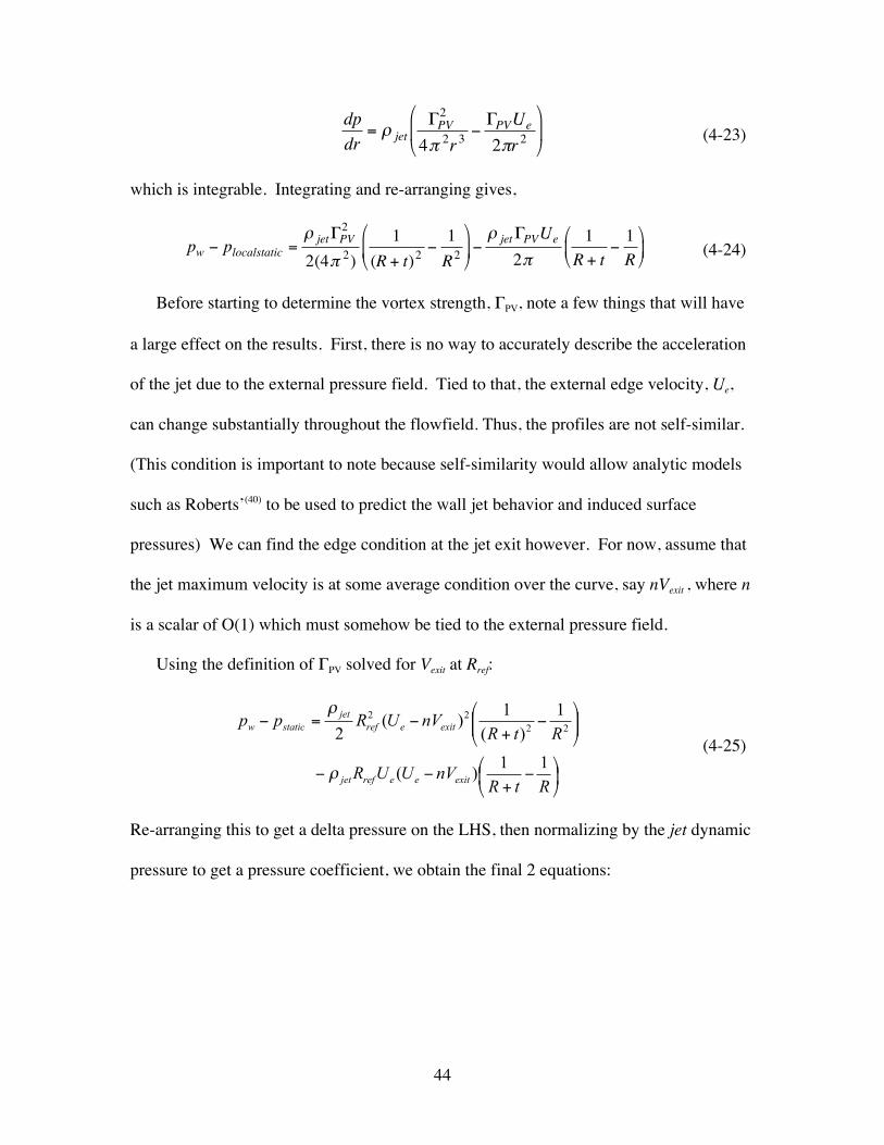
To model the jet at any given surface station, introduce a uniform velocity potential to
go with our point vortex as illustrated in Figure 4-7.
Figure 4-7: Sketch of jet velocity profiles with an external flow
From potential flow theory, the velocity is then:
€
V =Ue (x) −ΓPV2πr (4-22)
Following the same procedure as before:
44
€
dpdr
= ρ jetΓPV2
4π 2r 3−ΓPVUe
2πr 2
(4-23)
which is integrable. Integrating and re-arranging gives,
€
pw − plocalstatic =ρ jetΓPV
2
2(4π 2)1
(R + t)2−1R2
−
ρ jetΓPVUe
2π1
R + t−1R
(4-24)
Before starting to determine the vortex strength, ΓPV, note a few things that will have
a large effect on the results. First, there is no way to accurately describe the acceleration
of the jet due to the external pressure field. Tied to that, the external edge velocity, Ue,
can change substantially throughout the flowfield. Thus, the profiles are not self-similar.
(This condition is important to note because self-similarity would allow analytic models
such as Roberts’(40) to be used to predict the wall jet behavior and induced surface
pressures) We can find the edge condition at the jet exit however. For now, assume that
the jet maximum velocity is at some average condition over the curve, say nVexit , where n
is a scalar of O(1) which must somehow be tied to the external pressure field.
Using the definition of ΓPV solved for Vexit at Rref:
−+
−−
−
+−=−
RtRnVUUR
RtRnVURpp
exiteerefjet
exiterefjet
staticw
11)(
1)(
1)(
2 2222
ρ
ρ
(4-25)
Re-arranging this to get a delta pressure on the LHS, then normalizing by the jet dynamic
pressure to get a pressure coefficient, we obtain the final 2 equations:

45
−+
−−
−
+−+−=Δ ∞
RtRnVUUR
RtRnVURppp
exiteerefjet
exiterefjet
staticlocal
11)(
1)(
1)(
2)( 22
22
ρ
ρ
(4-26)
−+
−
−
−
+−+
= ∞
RtRVU
nVU
R
RtRn
VU
RCqq
C
exit
e
exit
eref
exit
erefedgep
jetp
112
1)(
1)(
2
2222
,
(4-27)
Note that equations (4-26) and (4-27) reduce to equations (4-20) and (4-21), respectively,
when the freestream velocity goes to zero.
Predictions from these equations can be compared with Davenport’s data. To
establish a comparison, estimate the local static pressure/local edge velocity from the
thickness of his experimental model, shown in Figure 4-5. For a q∞ of 12.5 lb/ft2, this
edge velocity is around 125.6 ft/s. Take the reference radius, Rref, to be R+t/2 since this
seems to correlate the data well (see Fig 4-5), and choose n to be 1.25. This means that
the jet is accelerated by about 25% around the curve by the external pressure field. This
number was used based on experimental velocity profiles taken from Davenport. Any
other numbers remain identical from previous computations and were taken directly from
his paper. The pressure along the curve is shown in Figure 4-7. Note that the surface
pressures are approximated well, and better agreement could be expected with better
information about the jet conditions.
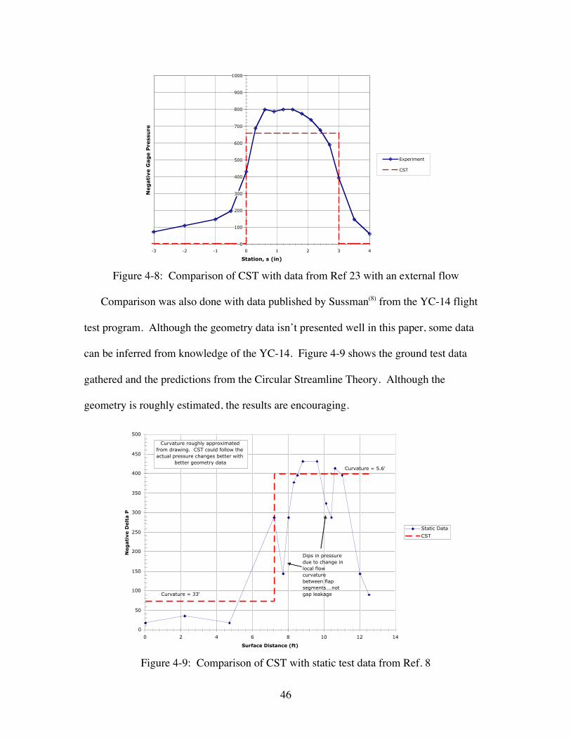
46
0
100
200
300
400
500
600
700
800
900
1000
-3 -2 -1 0 1 2 3 4
Station, s (in)
Neg
ati
ve G
ag
e P
ress
ure
Experiment
CST
Figure 4-8: Comparison of CST with data from Ref 23 with an external flow
Comparison was also done with data published by Sussman(8) from the YC-14 flight
test program. Although the geometry data isn’t presented well in this paper, some data
can be inferred from knowledge of the YC-14. Figure 4-9 shows the ground test data
gathered and the predictions from the Circular Streamline Theory. Although the
geometry is roughly estimated, the results are encouraging.
0
50
100
150
200
250
300
350
400
450
500
0 2 4 6 8 10 12 14
Surface Distance (ft)
Neg
ati
ve D
elt
a P
Static Data
CST
Dips in pressure due to change in local flow curvature between flap segments….not gap leakage
Curvature roughly approximated from drawing. CST could follow the actual pressure changes better with
better geometry data
Curvature = 33'
Curvature = 5.6'
Figure 4-9: Comparison of CST with static test data from Ref. 8
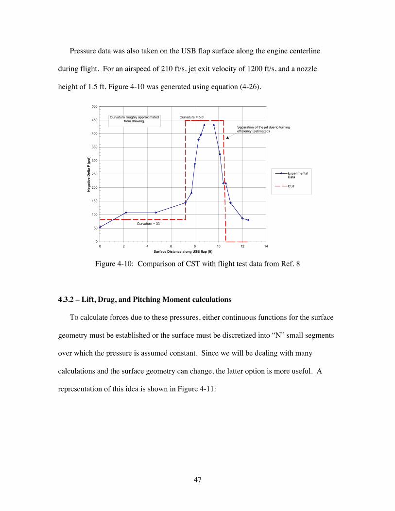
47
Pressure data was also taken on the USB flap surface along the engine centerline
during flight. For an airspeed of 210 ft/s, jet exit velocity of 1200 ft/s, and a nozzle
height of 1.5 ft, Figure 4-10 was generated using equation (4-26).
0
50
100
150
200
250
300
350
400
450
500
0 2 4 6 8 10 12 14
Surface Distance along USB flap (ft)
Neg
ativ
e D
elta
P (
psf
)
ExperimentalData
CST
Separation of the jet due to turning efficiency (estimated)
Curvature roughly approximated from drawing.
Curvature = 33'
Curvature = 5.6'
Figure 4-10: Comparison of CST with flight test data from Ref. 8
4.3.2 – Lift, Drag, and Pitching Moment calculations
To calculate forces due to these pressures, either continuous functions for the surface
geometry must be established or the surface must be discretized into “N” small segments
over which the pressure is assumed constant. Since we will be dealing with many
calculations and the surface geometry can change, the latter option is more useful. A
representation of this idea is shown in Figure 4-11:
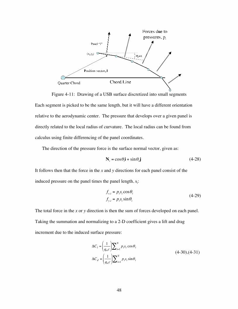
48
Figure 4-11: Drawing of a USB surface discretized into small segments
Each segment is picked to be the same length, but it will have a different orientation
relative to the aerodynamic center. The pressure that develops over a given panel is
directly related to the local radius of curvature. The local radius can be found from
calculus using finite differencing of the panel coordinates.
The direction of the pressure force is the surface normal vector, given as:
€
Ni = cosθii + sinθij (4-28)
It follows then that the force in the x and y directions for each panel consist of the
induced pressure on the panel times the panel length, si:
€
fx,i = pisi cosθify,i = pisi sinθi
(4-29)
The total force in the x or y direction is then the sum of forces developed on each panel.
Taking the summation and normalizing to a 2-D coefficient gives a lift and drag
increment due to the induced surface pressure:
€
ΔCl =1q∞c
pisi cosθ ii=1
N∑
ΔCd =1q∞c
pisi sinθ ii=1
N∑
(4-30),(4-31)
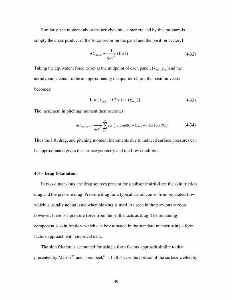
49
Similarly, the moment about the aerodynamic center created by this pressure is
simply the cross product of the force vector on the panel and the position vector, l.
€
ΔCm,ac =1
q∞c2 (F × l) (4-32)
Taking the equivalent force to act at the midpoint of each panel, (xm,i, ym,i)and the
aerodynamic center to be at approximately the quarter-chord, the position vector
becomes:
€
l i = (xm,i − 0.25c)i + (ym,i)j (4-33)
The increment in pitching moment then becomes:
€
ΔCm,0.25c =1
q∞c2 pisi ym,i sin(θ i) − (xm,i − 0.25c) cos(θ i)( )i=1
N
∑ (4-34)
Thus the lift, drag, and pitching moment increments due to induced surface pressures can
be approximated given the surface geometry and the flow conditions.
4.4 – Drag Estimation
In two-dimensions, the drag sources present for a subsonic airfoil are the skin friction
drag and the pressure drag. Pressure drag for a typical airfoil comes from separated flow,
which is usually not an issue when blowing is used. As seen in the previous section,
however, there is a pressure force from the jet that acts as drag. The remaining
component is skin friction, which can be estimated in the standard manner using a form
factors approach with empirical data.
The skin friction is accounted for using a form factors approach similar to that
presented by Mason(15) and Torenbeek(41). In this case the portion of the surface wetted by

50
the jet has a different skin friction coefficient. The friction drag coefficient (part of Cdo)
is:
€
Cd = CF, fsS fsSref
+CF, jet
S jetSref
FF (4-35)
where “fs” denotes normal flow and “jet” denotes the area exposed to the exhaust, and FF
represents the form factor of our airfoil. The skin friction coefficients are given by the
Prandtl-Schlichting formula:
€
CF =0.455
(log10(Rec ))2.58 (4-36)
The form factor used is:
€
FF = 1+1.8 tc( ) + 50 t
c( )4
(4-37)
For the pressure drag, a relation was established in equation (4-30) above. However,
as described in Chapter 2, not all of this drag will be realized. In fact, a large portion of it
can and will be balanced by leading edge suction. A simple multiplier can be applied to
equation (4-30) in that respect. Call this multiplier the “pressure drag factor” and denote
it by the variable, ζ. The determination of the magnitude of this multiplier is discussed in
the next chapter. Note that for the real-world situation, there can also exist a significant
form drag with no blowing. This quantity is not accounted for in this method.
4.5 – Entrainment Effects
The effects of entrainment are more difficult to quantify. At this point, there is no
established method for incorporating these types of effects for upper surface blown
configurations. The goal of this work is to provide enough empirical approximations of
these effects to correlate existing data. A set of experiments designed to measure

51
entrainment effects within the framework of the current prediction method would be the
next logical step, but that has not been done here.
Basically, the lift augmentation produced by direct fluid entrainment from the jet is
needed. For small amounts of blowing, we should also account for the positive lift and
drag effects produced by boundary layer control. Following the breakdown shown in
Chapter 2, a multiplicative factor is used on the lift to account for entrainment effects.
Call this factor, ηent. A full discussion of the development of this and other factors is
given in the following chapter. While the choice of these factors can be subjective and/or
sensitive to configuration, it will be shown that good correlation can be obtained via
relatively simple empirical relations.
4.6 – Total Two-Dimensional Equations for Lift, Drag, and Pitching Moment
Having developed the constituent pieces of the method, we can now present the total
equations for 2-D upper surface blowing performance characteristics. These equations
require only the specification of the jet exhaust conditions, nozzle parameters, surface
geometry, and freestream conditions. They provide estimations of the sectional lift, drag,
and pitching moment coefficients.
4.6.1 – Lift Coefficient
The 2-D lift coefficient is given by a combination of equations (4-9) and (4-29) and
the entrainment factor described above:
€
Cl = (1+ηent )2πα + 4πBoα + 2 χ + sinχ + 2πDo( )δ f + 4πγ 1+Co( )( )
+1q∞c
pisi cosθ ii=1
N∑
(4-38)

52
where all the quantities have been defined previously. The functional dependence can be
written as:
€
Cl = f α,γ ,E,δ f ,Cµ ,Rec ,Re jet ,nozzle geometry
where Rec and Rejet are the Reynolds numbers of the freestream and jet flow respectively.
4.6.2 – Pitching Moment Coefficient
The 2-D pitching moment coefficient is based on a combination of equations (4-
13),(4-15), and (4-34) above.
€
Cm,0.25c =14Cl,JetFlap + −
12πα + Eoα
−
12χ + sinχ +
14sin(2χ)
δ f +Goδ f
+
1q∞c
2 pisi ym,i sin(θ i) − (xm,i − 0.25c) cos(θ i)( )i=1
N
∑ (4-39)
This equation has the same functional dependence as the lift coefficient.
4.6.3 – Drag Coefficient
The 2-D drag coefficient is given by a combination of the equations (4-31), (4-35)
and the pressure drag factor.
€
Cd = CF, fsS fsSref
+CF, jet
S jetSref
* FF + ζ
1q∞c
pisi sinθ ii=1
N∑
(4-40)
where, again, S represents a surface length around the airfoil. The functional dependence
for the drag coefficient is very similar to the lift and pitching moment coefficients but
includes a dependence on the airfoil thickness, t/c.

53
Chapter 5: Correlation of 2-D method with Experimental Data
This chapter documents the correlation of the methodology outlined in the previous
chapter with published experimental data for 2-D USB configurations. The data used
was primarily taken from a series of experiments performed at the University of Texas at
Arlington(42),(43),(44). These experiments employed a modified, symmetric NACA airfoil
with a propulsive nozzle located on the aft portion of the upper surface. The lift and
pitching moments were recorded for various angles of attack and blowing coefficients.
The development of empirical relations for various factors is shown, and these factors are
seen to provide good correlation over a physically realistic range of blowing coefficients.
5.1 – Description of Published Experiments
5.1.1 – History and Overview
The propulsive wing concept was an ongoing research activity at the Aerodynamics
Research Center at the University of Texas at Arlington during the 1980s. These projects
were overseen by Dr. Don Wilson, with primary research being done by Roberts(42),
54
Pernice(43), and Jeon(44). The main purpose of this work was to provide two-dimensional
force and moment data for a propulsive wing system. A small-scale wing was built
which used compressed air exhausting over the aft portion of the upper surface to
simulate the engine flow. All researchers used modified NACA sections, and all were
symmetric with the exception of Roberts(42). Figure 5-1 shows the test article:
Figure 5-1: Propulsive wing section used in experiments by Jeon(44)
Pressure taps were located at the mid-span of the wing spaced around the full contour
of the section. Measurements were taken to ensure that the flow was sufficiently two-
dimensional at this location, given the small span (b < 1 ft) of the models involved.
Quadrature was used to get force and moment measurements from the pressure data.
Jeon also attempted to make drag measurements from the wake rake data. Since the
forces and moments were found from an integration of surface pressures, the jet reaction
lift is not included in the test data, nor is the skin friction drag. These omissions were
accounted for in the current calculations.

55
In addition to collecting force and moment data, much of the research involved the
search for correlation parameters for USB configurations. The goal was to find a
parameter or parameter grouping which correlated the lift coefficient linearly. It was
found that the velocity ratio between the jet and the external stream at the jet exit
provided a roughly linear correlation. However, this ratio is not very useful in a design
sense since the external velocity requires some work to obtain. The study of this type of
correlation parameter did, however, bring about a very useful study of the entrainment
ability of the exhaust jet. This information was helpful in developing empirical relations
in the current study.
The blowing coefficient, Cj, used in this work has a non-linear relationship with the
lift, as does the net thrust coefficient. (Recall that for a 2-D case, the blowing coefficient
is equivalent to the gross thrust coefficient) The non-linearity of Cl with Cj is evident in
the equations from jet-flap theory. In addition, Pernice(43) demonstrated that the blowing
coefficient provides a poor correlation of the data in cases where the jet velocity and
freestream velocity are roughly the same magnitude. However, such cases represent
infeasible designs because this condition indicates the propulsive system has zero net
thrust. The blowing coefficient provides a familiar, useful tie to the propulsion system
making it the most efficient correlation parameter for conceptual design despite the non-
linearity.
One drawback to the use of these experiments is that no work was done incorporating
deflected trailing edge flaps. It is expected that the presence of the flaps (if properly
contoured) would greatly increase the force and pitching moments. Flaps essentially
provide an increase in trailing edge flow angle and aft surface curvature. Their presence
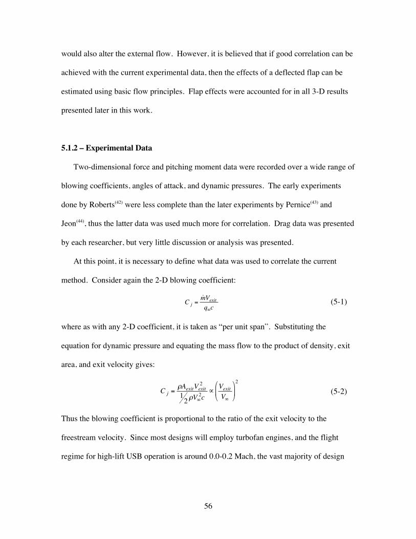
56
would also alter the external flow. However, it is believed that if good correlation can be
achieved with the current experimental data, then the effects of a deflected flap can be
estimated using basic flow principles. Flap effects were accounted for in all 3-D results
presented later in this work.
5.1.2 – Experimental Data
Two-dimensional force and pitching moment data were recorded over a wide range of
blowing coefficients, angles of attack, and dynamic pressures. The early experiments
done by Roberts(42) were less complete than the later experiments by Pernice(43) and
Jeon(44), thus the latter data was used much more for correlation. Drag data was presented
by each researcher, but very little discussion or analysis was presented.
At this point, it is necessary to define what data was used to correlate the current
method. Consider again the 2-D blowing coefficient:
€
C j =˙ m Vexitq∞c
(5-1)
where as with any 2-D coefficient, it is taken as “per unit span”. Substituting the
equation for dynamic pressure and equating the mass flow to the product of density, exit
area, and exit velocity gives:
€
C j =ρAexitVexit
2
12ρV∞
2c∝
VexitV∞
2
(5-2)
Thus the blowing coefficient is proportional to the ratio of the exit velocity to the
freestream velocity. Since most designs will employ turbofan engines, and the flight
regime for high-lift USB operation is around 0.0-0.2 Mach, the vast majority of design
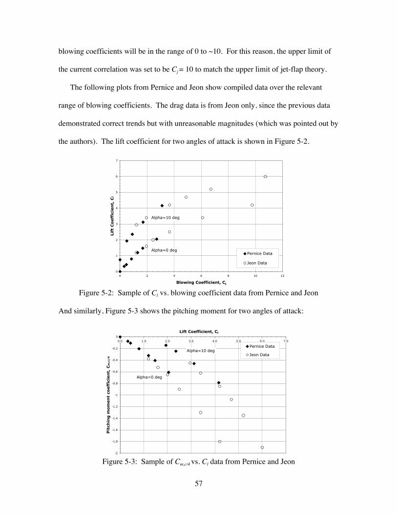
57
blowing coefficients will be in the range of 0 to ~10. For this reason, the upper limit of
the current correlation was set to be Cj = 10 to match the upper limit of jet-flap theory.
The following plots from Pernice and Jeon show compiled data over the relevant
range of blowing coefficients. The drag data is from Jeon only, since the previous data
demonstrated correct trends but with unreasonable magnitudes (which was pointed out by
the authors). The lift coefficient for two angles of attack is shown in Figure 5-2.
0
1
2
3
4
5
6
7
0 2 4 6 8 10 12
Blowing Coefficient, Cj
Lif
t C
oeff
icie
nt,
Cl
Pernice Data
Jeon Data
Alpha=0 deg
Alpha=10 deg
Figure 5-2: Sample of Cl vs. blowing coefficient data from Pernice and Jeon
And similarly, Figure 5-3 shows the pitching moment for two angles of attack:
-2
-1.8
-1.6
-1.4
-1.2
-1
-0.8
-0.6
-0.4
-0.2
0
0.0 1.0 2.0 3.0 4.0 5.0 6.0 7.0
Lift Coefficient, Cl
Pit
chin
g m
om
en
t co
eff
icie
nt,
Cm
,c/
4
Pernice Data
Jeon Data
Alpha=0 deg
Alpha=10 deg
Figure 5-3: Sample of Cm,c/4 vs. Cl data from Pernice and Jeon
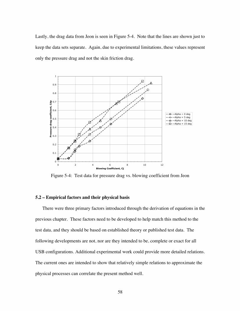
58
Lastly, the drag data from Jeon is seen in Figure 5-4. Note that the lines are shown just to
keep the data sets separate. Again, due to experimental limitations, these values represent
only the pressure drag and not the skin friction drag.
0
0.1
0.2
0.3
0.4
0.5
0.6
0.7
0.8
0.9
1
0 2 4 6 8 10 12
Blowing Coefficient, Cj
Pre
ssu
re d
rag
co
eff
icie
nt,
Cd
p
Alpha = 0 degAlpha = 5 degAlpha = 10 degAlpha = 15 deg
Figure 5-4: Test data for pressure drag vs. blowing coefficient from Jeon
5.2 – Empirical factors and their physical basis
There were three primary factors introduced through the derivation of equations in the
previous chapter. These factors need to be developed to help match this method to the
test data, and they should be based on established theory or published test data. The
following developments are not, nor are they intended to be, complete or exact for all
USB configurations. Additional experimental work could provide more detailed relations.
The current ones are intended to show that relatively simple relations to approximate the
physical processes can correlate the present method well.

59
5.2.1 – The n factor
This factor comes from the Circular Streamline Theory. Recall that there are low
pressures directly induced by the curved wall jet flowing over the aft surface. An
approximate equation for these pressures was derived in Chapter 4, equation (4-26). It is
shown again here, ignoring the relatively small difference between freestream pressure
and the local static near the jet exit:
€
p =ρ jet
2Rref2 (Ue − nVexit )
2 1(R + t)2
−1R2
− ρ jetRrefUe (Ue − nVexit )
1R + t
−1R
(5-3)
Here n is a “jet acceleration” factor. Essentially, this factor relates the behavior of the jet
and the freestream conditions. This factor allows slight adjustment of the exit condition in
an average sense to account for the external flow.
Davenport(24) says, “A considerable increase in jet velocity over the value at the
nozzle exit is seen as the jet rounds a corner, especially at forward speeds where the jet is
expanding into the low pressure region created by the outside flow field”. The only data
he presented showed a maximum increase of about 25 to 30% in jet velocity with a
deflected flap. One can expect that this factor is a strong function of angle of attack and
flap deflection. This factor will increase the force by decreasing the aft pressure, but it
should not be allowed to become large, since this would make the pitching moments
become too large.
With this in mind, a simple linear relation is suggested for the “n” factor:
€
n = 1.0+α(deg)100
+
δ f (deg)500
(5-4)
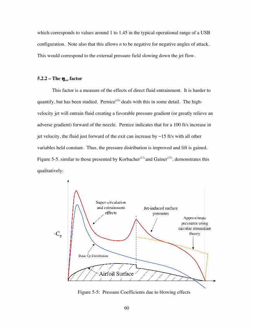
60
which corresponds to values around 1 to 1.45 in the typical operational range of a USB
configuration. Note also that this allows n to be negative for negative angles of attack.
This would correspond to the external pressure field slowing down the jet flow.
5.2.2 – The ηent factor
This factor is a measure of the effects of direct fluid entrainment. It is harder to
quantify, but has been studied. Pernice(43) deals with this in some detail. The high-
velocity jet will entrain fluid creating a favorable pressure gradient (or greatly relieve an
adverse gradient) forward of the nozzle. Pernice indicates that for a 100 ft/s increase in
jet velocity, the fluid just forward of the exit can increase by ~15 ft/s with all other
variables held constant. Thus, the pressure distribution is improved and lift is gained.
Figure 5-5, similar to those presented by Korbacher(17) and Gainer(37), demonstrates this
qualitatively:
Figure 5-5: Pressure Coefficients due to blowing effects

61
It is expected that this effect is primarily a function of the blowing coefficient. Recall
from Chapter 4 that the entrainment factor modifies the total lift coefficient as:
€
Cl = (1+ηent )(Cl,JetFlap +Cl,Jet Pressure) (5-5)
In general, (and certainly for this data) this effect will not contribute significantly to the
pitching moment. Based upon the fact that Pernice found a linear relation between the
effective velocity ratio (Vjet,exit/Vexternal,exit) and the lift, the following function is initially
suggested:
€
ηent = 0.05C j (5-6)
However, this factor can also be used to account for boundary layer control effects
(BLC). These effects were described by Korbacher(17). Essentially, these are the strong
initial effects of blowing. For small blowing coefficients, the primary effect is to relieve
adverse pressure gradients and eliminate separation. This is the steep increase in lift at
small blowing coefficients seen in the sample data of Figure 5-2. Also, as the angle of
attack increases, this initial slope increases. Consider the BLC effect to be allowing the
airfoil to reach its potential since adverse gradients/separation become more prevalent for
an airfoil with increasing angle of attack. The curves in Figure 5-2 could be
approximately described by 2 linear functions. This idea is supported by work done by
Roberts(42), who suggested a piecewise-linear fit to the data with the slopes/intercepts
being determined empirically.
From a physical standpoint and also a programming standpoint, it makes sense to roll
this effect into the “entrainment factor”. For a small region of low blowing coefficients
(say Cj <0.8), a multiplicative factor, say λBLC, is added to ηent to reflect the sharp increase
in lift capability. Thus, equation (5-6) becomes:
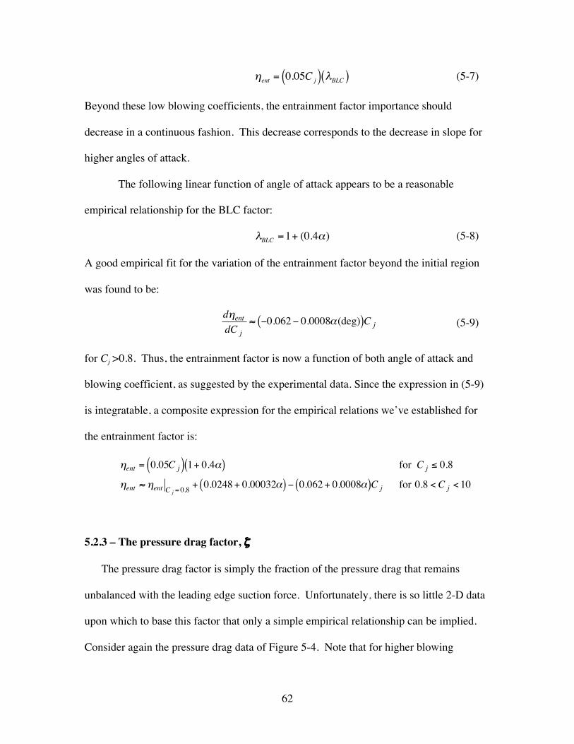
62
€
ηent = 0.05C j( ) λBLC( ) (5-7)
Beyond these low blowing coefficients, the entrainment factor importance should
decrease in a continuous fashion. This decrease corresponds to the decrease in slope for
higher angles of attack.
The following linear function of angle of attack appears to be a reasonable
empirical relationship for the BLC factor:
€
λBLC =1+ (0.4α) (5-8)
A good empirical fit for the variation of the entrainment factor beyond the initial region
was found to be:
€
dηentdC j
≈ −0.062− 0.0008α(deg)( )C j (5-9)
for Cj >0.8. Thus, the entrainment factor is now a function of both angle of attack and
blowing coefficient, as suggested by the experimental data. Since the expression in (5-9)
is integratable, a composite expression for the empirical relations we’ve established for
the entrainment factor is:
€
ηent = 0.05C j( ) 1+ 0.4α( ) for C j ≤ 0.8
ηent ≈ ηent C j = 0.8 + 0.0248 + 0.00032α( ) − 0.062 + 0.0008α( )C j for 0.8 < C j < 10
5.2.3 – The pressure drag factor, ζ
The pressure drag factor is simply the fraction of the pressure drag that remains
unbalanced with the leading edge suction force. Unfortunately, there is so little 2-D data
upon which to base this factor that only a simple empirical relationship can be implied.
Consider again the pressure drag data of Figure 5-4. Note that for higher blowing

63
coefficients, the rate of increase in the pressure drag is roughly equivalent for all angles
of attack.
For smaller blowing coefficients, the lesser angles of attack actually experience a
drag decrease with blowing. This goes back to the BLC concept. A typical USB
configuration (see Figure 5-1) will have a large form drag penalty when no blowing is
used. Thus, when blowing begins, it “cleans up” the flow separation and produces
improved drag values. This effect is eventually over-shadowed by the high pressures
induced on the aft surface and drag begins to increase.
To avoid over-complication, the drag bucket caused by BLC will not be modeled.
This is because not enough information is available to fully describe it. This omission
will only move the resulting approximations to the conservative side in that the drag for
low blowing coefficients will be slightly over-predicted. The pressure drag factor, ζ, can
be modeled in several ways. One way is to create a linear function of Cj to describe the
fraction. A second way is to simply assign the factor to a constant fractional value across
the range of blowing coefficients. For the former, a reasonable fit to the data is:
€
ζ = −0.06875C j( ) + 0.9875 (5-11)
and for the latter, reasonable values could range from 0.3 to 0.5. In other words, 30 to
50% of the aft pressure force is being realized as drag.
5.3 – Presentation of 2-D Correlation
The following plots show a comparison of the current USB methodology and the
classical jet-flap theory with the published data described above. The current method
consists of equations (4-38) through (4-40) of Chapter 4, coupled with the empirical
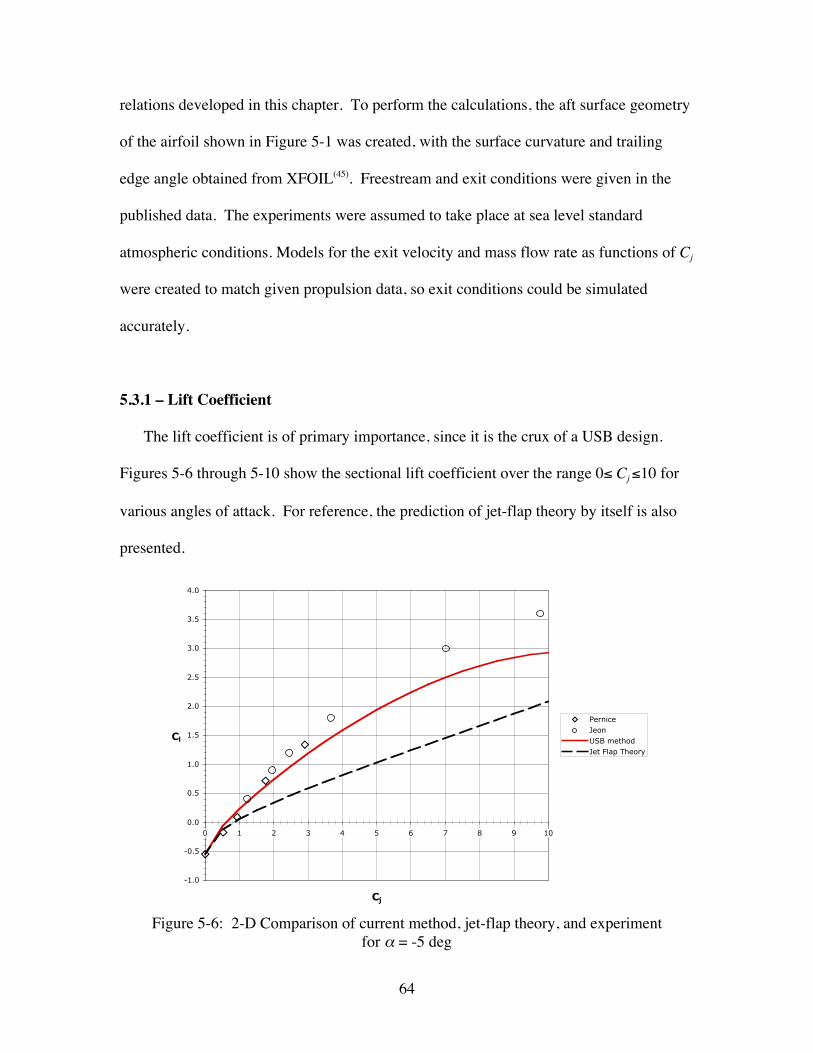
64
relations developed in this chapter. To perform the calculations, the aft surface geometry
of the airfoil shown in Figure 5-1 was created, with the surface curvature and trailing
edge angle obtained from XFOIL(45). Freestream and exit conditions were given in the
published data. The experiments were assumed to take place at sea level standard
atmospheric conditions. Models for the exit velocity and mass flow rate as functions of Cj
were created to match given propulsion data, so exit conditions could be simulated
accurately.
5.3.1 – Lift Coefficient
The lift coefficient is of primary importance, since it is the crux of a USB design.
Figures 5-6 through 5-10 show the sectional lift coefficient over the range 0≤ Cj ≤10 for
various angles of attack. For reference, the prediction of jet-flap theory by itself is also
presented.
-1.0
-0.5
0.0
0.5
1.0
1.5
2.0
2.5
3.0
3.5
4.0
0 1 2 3 4 5 6 7 8 9 10
Cj
Cl
PerniceJeonUSB methodJet Flap Theory
Figure 5-6: 2-D Comparison of current method, jet-flap theory, and experimentfor α = -5 deg
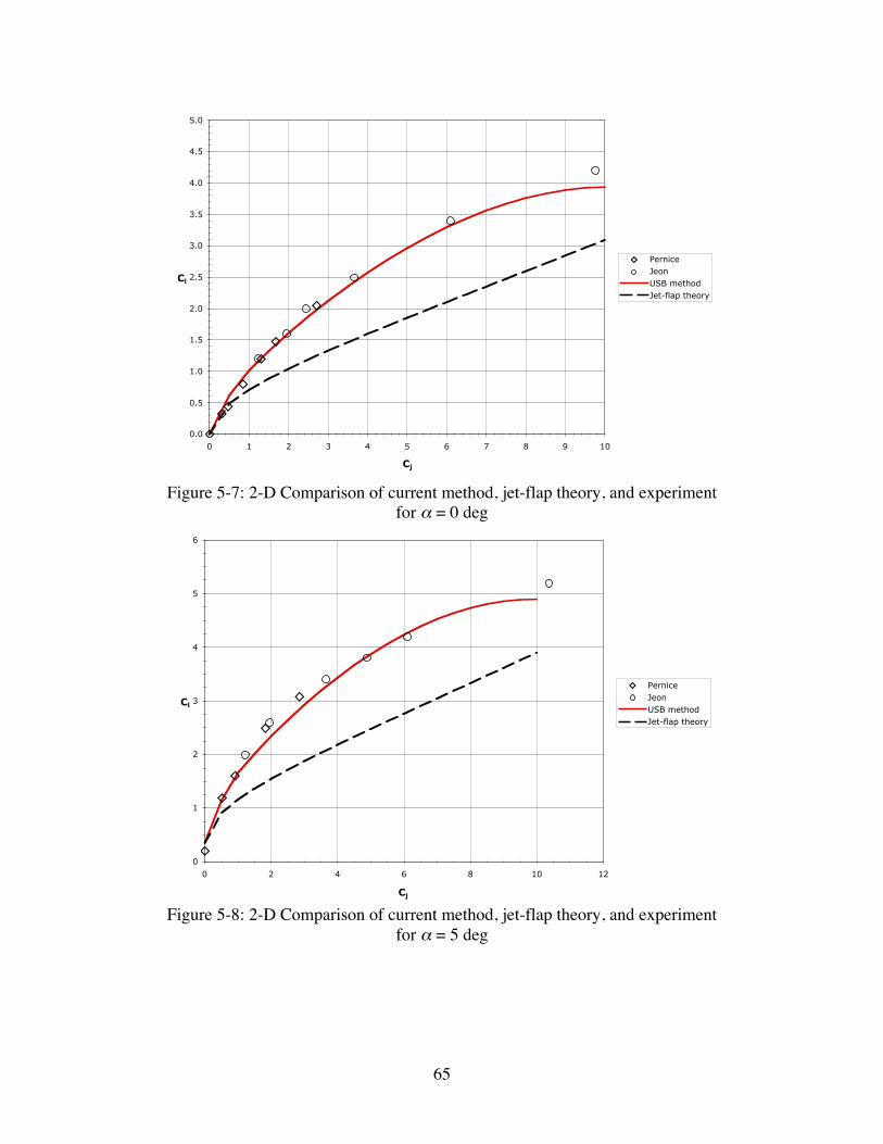
65
0.0
0.5
1.0
1.5
2.0
2.5
3.0
3.5
4.0
4.5
5.0
0 1 2 3 4 5 6 7 8 9 10
Cj
Cl
PerniceJeonUSB methodJet-flap theory
Figure 5-7: 2-D Comparison of current method, jet-flap theory, and experimentfor α = 0 deg
0
1
2
3
4
5
6
0 2 4 6 8 10 12
Cj
Cl
PerniceJeonUSB methodJet-flap theory
Figure 5-8: 2-D Comparison of current method, jet-flap theory, and experimentfor α = 5 deg
66
0
1
2
3
4
5
6
7
0 2 4 6 8 10 12
Cj
Cl
PerniceJeonUSB methodJet-flap theory
Figure 5-9: 2-D Comparison of current method, jet-flap theory, and experimentfor α = 10 deg
0
1
2
3
4
5
6
7
8
0 1 2 3 4 5 6 7 8 9 10
Cj
Cl
PerniceJeonUSB methodJet-flap theory
Figure 5-10: 2-D Comparison of current method, jet-flap theory, and experimentfor α = 15 deg
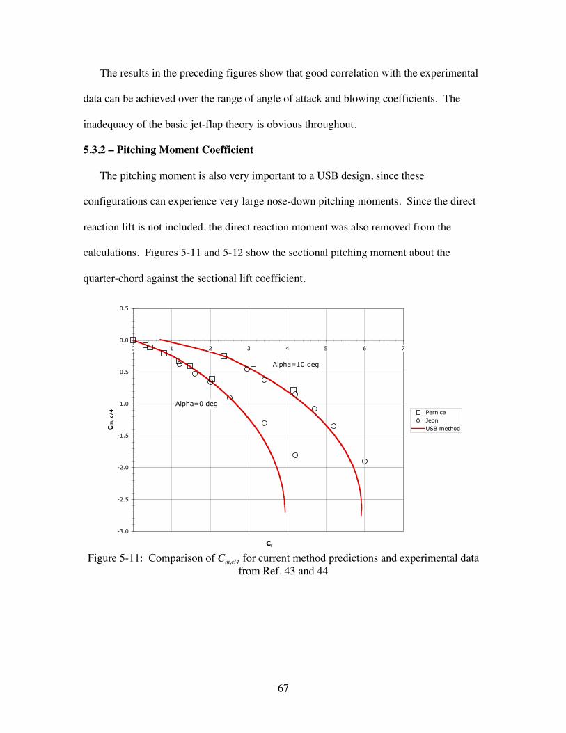
67
The results in the preceding figures show that good correlation with the experimental
data can be achieved over the range of angle of attack and blowing coefficients. The
inadequacy of the basic jet-flap theory is obvious throughout.
5.3.2 – Pitching Moment Coefficient
The pitching moment is also very important to a USB design, since these
configurations can experience very large nose-down pitching moments. Since the direct
reaction lift is not included, the direct reaction moment was also removed from the
calculations. Figures 5-11 and 5-12 show the sectional pitching moment about the
quarter-chord against the sectional lift coefficient.
-3.0
-2.5
-2.0
-1.5
-1.0
-0.5
0.0
0.5
0 1 2 3 4 5 6 7
Cl
Cm
, c/
4 PerniceJeonUSB method
Alpha=0 deg
Alpha=10 deg
Figure 5-11: Comparison of Cm,c/4 for current method predictions and experimental datafrom Ref. 43 and 44
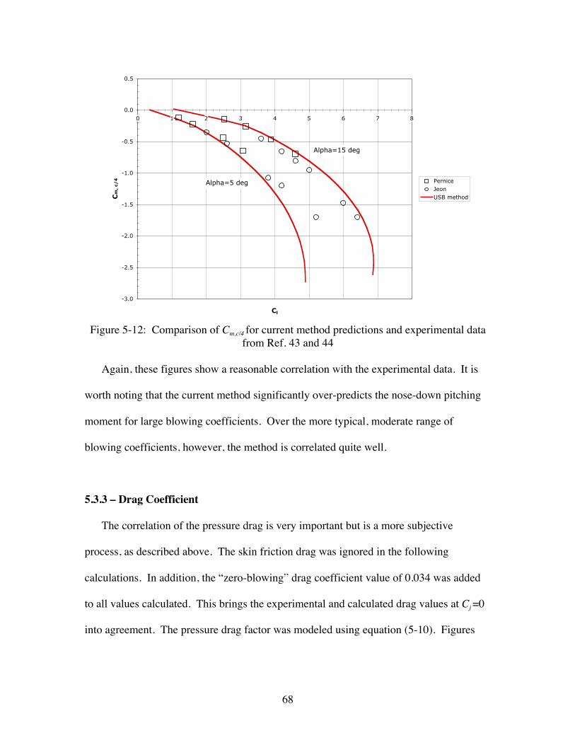
68
-3.0
-2.5
-2.0
-1.5
-1.0
-0.5
0.0
0.5
0 1 2 3 4 5 6 7 8
Cl
Cm
, c/
4 PerniceJeonUSB method
Alpha=5 deg
Alpha=15 deg
Figure 5-12: Comparison of Cm,c/4 for current method predictions and experimental datafrom Ref. 43 and 44
Again, these figures show a reasonable correlation with the experimental data. It is
worth noting that the current method significantly over-predicts the nose-down pitching
moment for large blowing coefficients. Over the more typical, moderate range of
blowing coefficients, however, the method is correlated quite well.
5.3.3 – Drag Coefficient
The correlation of the pressure drag is very important but is a more subjective
process, as described above. The skin friction drag was ignored in the following
calculations. In addition, the “zero-blowing” drag coefficient value of 0.034 was added
to all values calculated. This brings the experimental and calculated drag values at Cj =0
into agreement. The pressure drag factor was modeled using equation (5-10). Figures
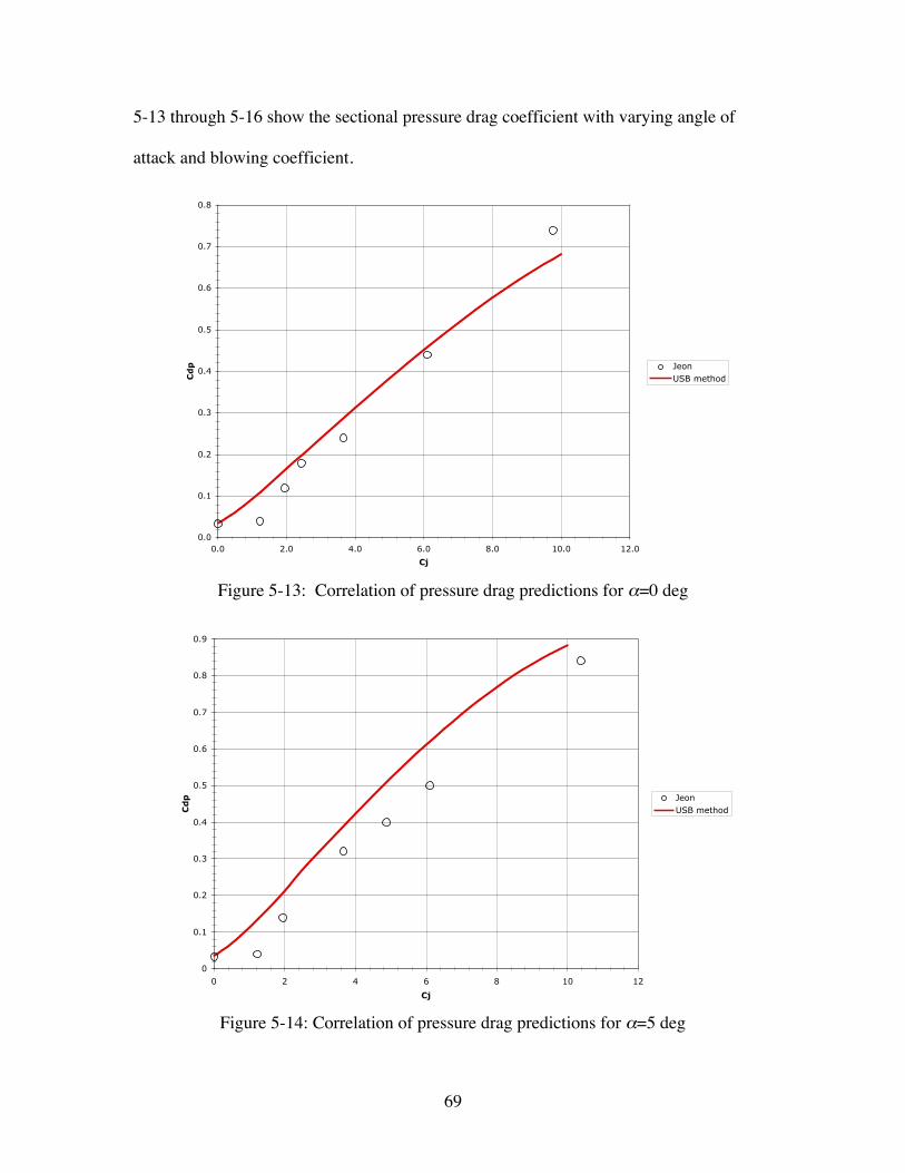
69
5-13 through 5-16 show the sectional pressure drag coefficient with varying angle of
attack and blowing coefficient.
0.0
0.1
0.2
0.3
0.4
0.5
0.6
0.7
0.8
0.0 2.0 4.0 6.0 8.0 10.0 12.0
Cj
Cdp Jeon
USB method
Figure 5-13: Correlation of pressure drag predictions for α=0 deg
0
0.1
0.2
0.3
0.4
0.5
0.6
0.7
0.8
0.9
0 2 4 6 8 10 12
Cj
Cdp Jeon
USB method
Figure 5-14: Correlation of pressure drag predictions for α=5 deg
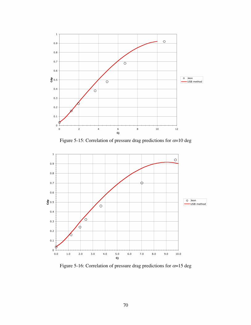
70
0
0.1
0.2
0.3
0.4
0.5
0.6
0.7
0.8
0.9
1
0 2 4 6 8 10 12
Cj
Cdp Jeon
USB method
Figure 5-15: Correlation of pressure drag predictions for α=10 deg
0
0.1
0.2
0.3
0.4
0.5
0.6
0.7
0.8
0.9
1
0.0 1.0 2.0 3.0 4.0 5.0 6.0 7.0 8.0 9.0 10.0
Cj
Cdp Jeon
USB method
Figure 5-16: Correlation of pressure drag predictions for α=15 deg

71
While the correlation is not as good for the pressure drag coefficients, this is not
unexpected. Again, since the drag is slightly over-predicted across the board, this makes
the estimate conservative.

72
Chapter 6: Three-Dimensional USB Performance Prediction Method
This chapter describes the method for estimating 3-D aerodynamic characteristics
using the 2-D approximate method developed in the previous chapters. The estimated
2-D values are used directly in an implementation of the Weissinger lifting line
method(46). The fundamentals of this method will be discussed along with its limitations.
In addition, the process of going from 2-D to 3-D will be discussed for a general USB
configuration. Finally, the additional potential of this method to provide information
about engine-out conditions will be examined.
6.1 – Overview of Weissinger Method
For the basic calculation of the aerodynamic performance of a wing at low speed, two
primary approaches are available. This first is “lifting line” theory and the second is the
“vortex lattice” method. The Weissinger method can be thought of as a cross between
these two in that it uses a distribution on bound vortices along the quarter-chord of the
wing, but it segments the wing into chordwise “strips” or panels. Flow tangency is then
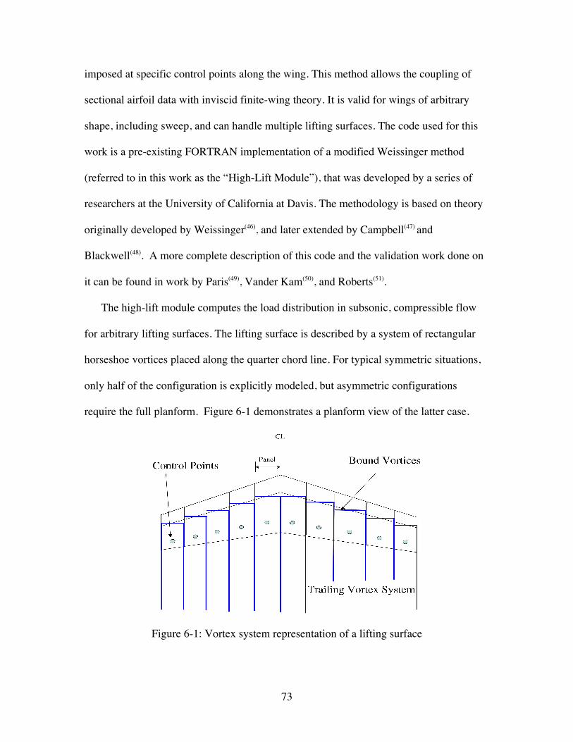
73
imposed at specific control points along the wing. This method allows the coupling of
sectional airfoil data with inviscid finite-wing theory. It is valid for wings of arbitrary
shape, including sweep, and can handle multiple lifting surfaces. The code used for this
work is a pre-existing FORTRAN implementation of a modified Weissinger method
(referred to in this work as the “High-Lift Module”), that was developed by a series of
researchers at the University of California at Davis. The methodology is based on theory
originally developed by Weissinger(46), and later extended by Campbell(47) and
Blackwell(48). A more complete description of this code and the validation work done on
it can be found in work by Paris(49), Vander Kam(50), and Roberts(51).
The high-lift module computes the load distribution in subsonic, compressible flow
for arbitrary lifting surfaces. The lifting surface is described by a system of rectangular
horseshoe vortices placed along the quarter chord line. For typical symmetric situations,
only half of the configuration is explicitly modeled, but asymmetric configurations
require the full planform. Figure 6-1 demonstrates a planform view of the latter case.
Figure 6-1: Vortex system representation of a lifting surface

74
The load distribution is calculated by solving for the N unknown vortex strengths while
imposing flow tangency conditions at the N control points. This is very similar to a vortex
lattice method, but here there is only one chordwise panel.
Although the high-lift module reduces the lifting surfaces to “strips” of flat plates,
various airfoil sections can be modeled. This includes any basic single-element airfoil,
high-lift airfoils, and in the present case, blown airfoils. The modeling of different airfoils
is accomplished by controlling the location of the control point and the effective
incidence of the panel. The location of the control point can be shifted from the standard
0.75c to reflect the appropriate lift-curve slope, and the panel incidence can be shifted to
reflect the zero-lift angle of attack of the section. Thus, portions of the wing with flaps
will be treated differently than an unflapped portion based on the difference in the
corresponding 2-D polars. The high-lift module also has the capability of taking viscous
2-D polars and predicting wing stall. This feature was not utilized in this work for reasons
that will be described in later sections.
Once the N-dimensional linear system has been solved, the total aerodynamic
coefficients can be calculated. The lift coefficient, CL, is integrated directly from the
calculated load distribution. The drag coefficient, CD, is composed of the induced drag
and parasite drag. The former is calculated using a Trefftz plane approach. The parasite
drag is essentially the drag value specified by the sectional data and can be integrated
along the span to get a total coefficient. The pitching moment coefficient, CM, is
calculated about a specified reference line (generally taken to be the aircraft center of
gravity) by integrating the sectional pitching moments across the span. The sectional
moments are transferred to the reference line by the following equation from Ref 49:
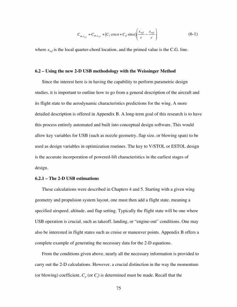
75
€
Cm,xref'= Cm,xref + Cl cosα +Cd sinα( )
xref'
c−xrefc
(6-1)
where xref is the local quarter-chord location, and the primed value is the C.G. line.
6.2 – Using the new 2-D USB methodology with the Weissinger Method
Since the interest here is in having the capability to perform parametric design
studies, it is important to outline how to go from a general description of the aircraft and
its flight state to the aerodynamic characteristics predictions for the wing. A more
detailed description is offered in Appendix B. A long-term goal of this research is to have
this process entirely automated and built into conceptual design software. This would
allow key variables for USB (such as nozzle geometry, flap size, or blowing span) to be
used as design variables in optimization routines. The key to V/STOL or ESTOL design
is the accurate incorporation of powered-lift characteristics in the earliest stages of
design.
6.2.1 – The 2-D USB estimations
These calculations were described in Chapters 4 and 5. Starting with a given wing
geometry and propulsion system layout, one must then add a flight state, meaning a
specified airspeed, altitude, and flap setting. Typically the flight state will be one where
USB operation is crucial, such as takeoff, landing, or “engine-out” conditions. One may
also be interested in flight states such as cruise or maneuver points. Appendix B offers a
complete example of generating the necessary data for the 2-D equations.
From the conditions given above, nearly all the necessary information is provided to
carry out the 2-D calculations. However, a crucial distinction in the way the momentum
(or blowing) coefficient, Cµ (or Cj) is determined must be made. Recall that the
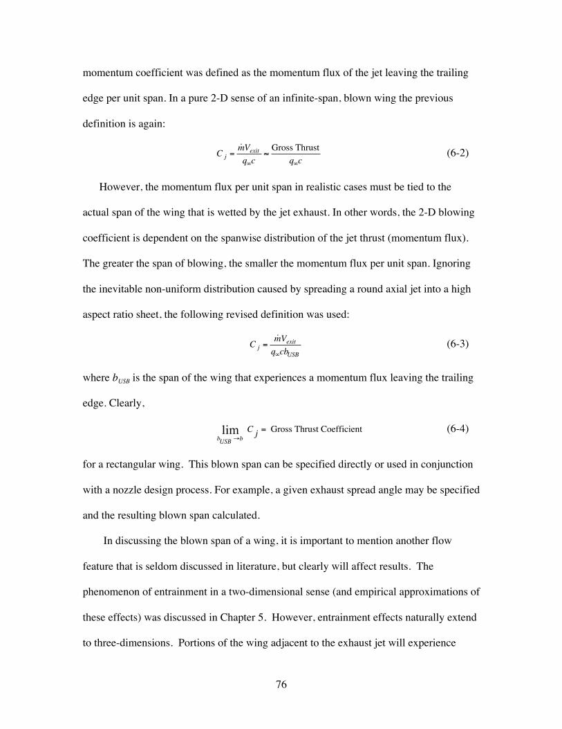
76
momentum coefficient was defined as the momentum flux of the jet leaving the trailing
edge per unit span. In a pure 2-D sense of an infinite-span, blown wing the previous
definition is again:
€
C j =˙ m Vexitq∞c
≈Gross Thrust
q∞c(6-2)
However, the momentum flux per unit span in realistic cases must be tied to the
actual span of the wing that is wetted by the jet exhaust. In other words, the 2-D blowing
coefficient is dependent on the spanwise distribution of the jet thrust (momentum flux).
The greater the span of blowing, the smaller the momentum flux per unit span. Ignoring
the inevitable non-uniform distribution caused by spreading a round axial jet into a high
aspect ratio sheet, the following revised definition was used:
€
C j =˙ m Vexit
q∞cbUSB(6-3)
where bUSB is the span of the wing that experiences a momentum flux leaving the trailing
edge. Clearly,
€
bUSB →blim C j = Gross Thrust Coefficient (6-4)
for a rectangular wing. This blown span can be specified directly or used in conjunction
with a nozzle design process. For example, a given exhaust spread angle may be specified
and the resulting blown span calculated.
In discussing the blown span of a wing, it is important to mention another flow
feature that is seldom discussed in literature, but clearly will affect results. The
phenomenon of entrainment in a two-dimensional sense (and empirical approximations of
these effects) was discussed in Chapter 5. However, entrainment effects naturally extend
to three-dimensions. Portions of the wing adjacent to the exhaust jet will experience
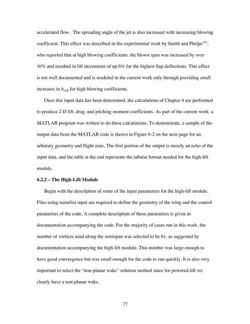
77
accelerated flow. The spreading angle of the jet is also increased with increasing blowing
coefficient. This effect was described in the experimental work by Smith and Phelps(54),
who reported that at high blowing coefficients, the blown span was increased by over
10% and resulted in lift increments of up 6% for the highest flap deflections. This effect
is not well documented and is modeled in the current work only through providing small
increases in bUSB for high blowing coefficients.
Once this input data has been determined, the calculations of Chapter 4 are performed
to produce 2-D lift, drag, and pitching moment coefficients. As part of the current work, a
MATLAB program was written to do these calculations. To demonstrate, a sample of the
output data from the MATLAB code is shown in Figure 6-2 on the next page for an
arbitrary geometry and flight state. The first portion of the output is merely an echo of the
input data, and the table at the end represents the tabular format needed for the high-lift
module.
6.2.2 – The High-Lift Module
Begin with the description of some of the input parameters for the high-lift module.
Files using namelist input are required to define the geometry of the wing and the control
parameters of the code. A complete description of these parameters is given in
documentation accompanying the code. For the majority of cases run in this work, the
number of vortices used along the semispan was selected to be 61, as suggested by
documentation accompanying the high-lift module. This number was large enough to
have good convergence but was small enough for the code to run quickly. It is also very
important to select the “non-planar wake” solution method since for powered-lift we
clearly have a non-planar wake.
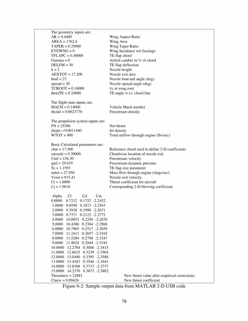
78
The geometry inputs are: AR = 9.4400 Wing Aspect Ratio
AREA = 1762.4 Wing AreaTAPER = 0.35000 Wing Taper RatioEYEWNG = 0 Wing Incidence wrt fuselageTFLAPC = 0.30000 TE flap chordGamma = 0 Airfoil camber in % of chordDELFM = 30 TE flap deflectionh = 2 Nozzle heightAEXTOT = 17.200 Nozzle exit areabtail = 23 Nozzle boat-tail angle (deg)spread = 20 Nozzle spread angle (deg)TCROOT = 0.16000 t/c at wing rootthetaTE = 0.24000 TE angle w.r.t. chord line
The flight state inputs are: MACH = 0.14000 Vehicle Mach number
rhoinf = 0.0023770 Freestream density
The propulsion system inputs are: FN = 25586 Net thrust
rhojet = 0.0011440 Jet densityWTOT = 900 Total airflow through engine (lbs/sec)
Basic Calculated parameters are: cbar = 17.500 Reference chord used to define 2-D coefficients
xnozzle = 0.30000 Chordwise location of nozzle exitUinf = 156.30 Freestream velocityqinf = 29.035 Freestream dynamic pressureXi = 1.1593 TE flap size parametermdot = 27.950 Mass flow through engine (slugs/sec)Vexit = 915.41 Nozzle exit velocityCt = 1.0000 Thrust coefficient for aircraftCj = 1.9618 Corresponding 2-D blowing coefficient
Alpha Cl Cd Cm0.0000 8.7212 0.1752 -2.2452 1.0000 9.0550 0.1873 -2.2563 2.0000 9.3938 0.1998 -2.2671 3.0000 9.7371 0.2123 -2.2772 4.0000 10.0853 0.2250 -2.2870 5.0000 10.4386 0.2384 -2.2968 6.0000 10.7965 0.2517 -2.3059 7.0000 11.1611 0.2657 -2.3165 8.0000 11.5284 0.2798 -2.3247 9.0000 11.9024 0.2944 -2.334510.0000 12.2784 0.3086 -2.341511.0000 12.6615 0.3239 -2.350412.0000 13.0490 0.3395 -2.358813.0000 13.4383 0.3546 -2.364114.0000 13.8368 0.3713 -2.373715.0000 14.2370 0.3873 -2.3802Thrustnew = 22881 New thrust value after empirical correctionsCtnew = 0.89426 New thrust coefficient
Figure 6-2: Sample output data from MATLAB 2-D USB code

79
A separate file allows the user to specify the airfoil sectional data for different
portions of the span. For any given spanwise location, the relevant polar is taken to be a
linear interpolation between the 2-D data defined at stations bracketing the point. So,
entering duplicate data at consecutive spanwise points means that all stations between
those points will use identical polar data. As described above, the polars for USB sections
are provided by the MATLAB code and are used directly in the high-lift module.
Non-blown sectional data was taken from various sources. Unfortunately, sectional
polars for multi-element airfoil sections are not readily available. To model this type of
data, lift increments were calculated using empirical methods like those from Raymer(52).
Although this introduces some error into the calculations, the magnitude of the error is
small due to the relative magnitude of the polars between the blown and un-blown
sections. Basic unblown airfoil data was generally obtained from Abbott and Von
Doenhoff(53).
6.3 – Limitations of Method
The limitations of the 2-D USB calculations have been discussed previously. These
limitations are primarily due to the breakdown of empirical approximations within the
method. They may also correspond to the inability to completely model the interactions
between the jet and the external flow. Thus, we can expect any approximation to
deteriorate with very large blowing coefficients and/or very large flap deflections.
Another fundamental consideration is that the methodology described in this work is for
inviscid flow. Although viscous corrections are being made, the calculations will never
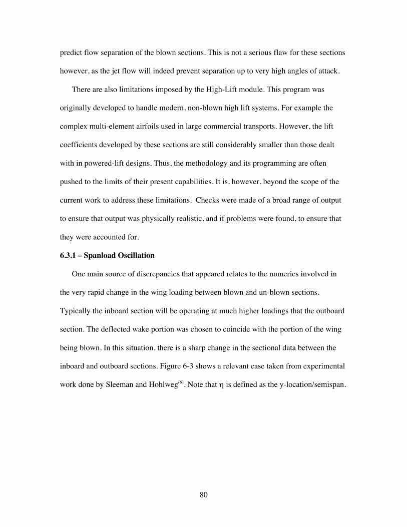
80
predict flow separation of the blown sections. This is not a serious flaw for these sections
however, as the jet flow will indeed prevent separation up to very high angles of attack.
There are also limitations imposed by the High-Lift module. This program was
originally developed to handle modern, non-blown high lift systems. For example the
complex multi-element airfoils used in large commercial transports. However, the lift
coefficients developed by these sections are still considerably smaller than those dealt
with in powered-lift designs. Thus, the methodology and its programming are often
pushed to the limits of their present capabilities. It is, however, beyond the scope of the
current work to address these limitations. Checks were made of a broad range of output
to ensure that output was physically realistic, and if problems were found, to ensure that
they were accounted for.
6.3.1 – Spanload Oscillation
One main source of discrepancies that appeared relates to the numerics involved in
the very rapid change in the wing loading between blown and un-blown sections.
Typically the inboard section will be operating at much higher loadings that the outboard
section. The deflected wake portion was chosen to coincide with the portion of the wing
being blown. In this situation, there is a sharp change in the sectional data between the
inboard and outboard sections. Figure 6-3 shows a relevant case taken from experimental
work done by Sleeman and Hohlweg(6). Note that η is defined as the y-location/semispan.
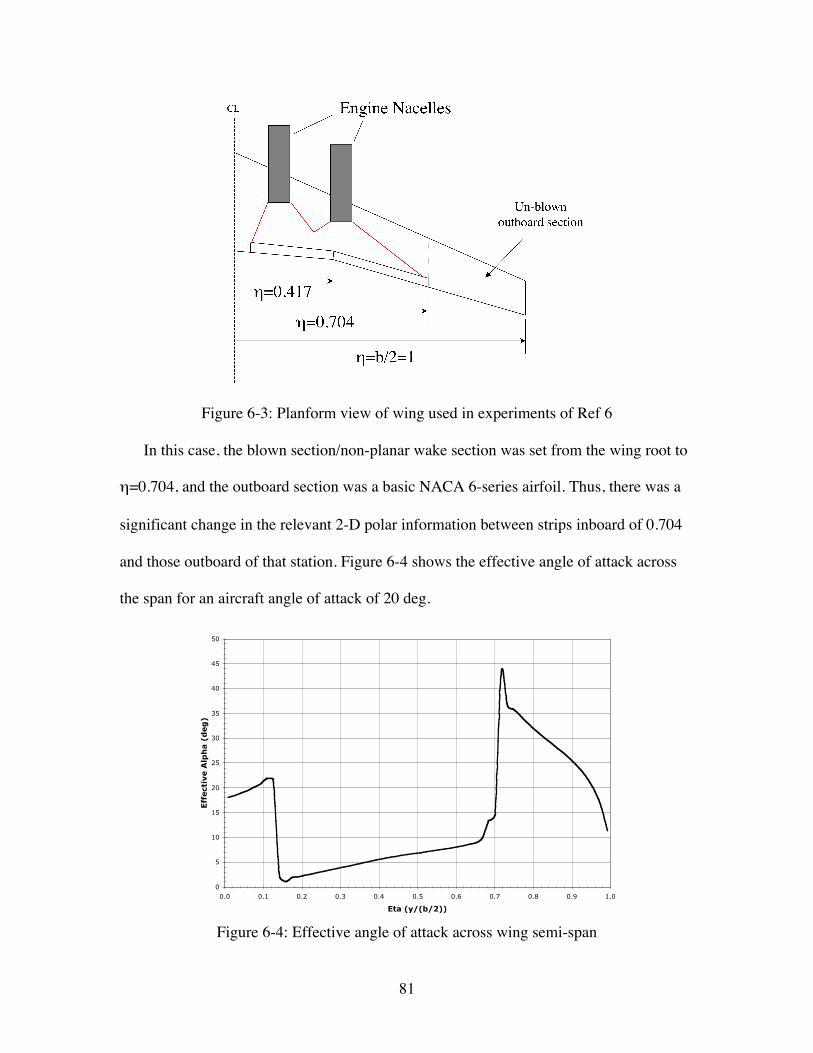
81
Figure 6-3: Planform view of wing used in experiments of Ref 6
In this case, the blown section/non-planar wake section was set from the wing root to
η=0.704, and the outboard section was a basic NACA 6-series airfoil. Thus, there was a
significant change in the relevant 2-D polar information between strips inboard of 0.704
and those outboard of that station. Figure 6-4 shows the effective angle of attack across
the span for an aircraft angle of attack of 20 deg.
0
5
10
15
20
25
30
35
40
45
50
0.0 0.1 0.2 0.3 0.4 0.5 0.6 0.7 0.8 0.9 1.0
Eta (y/(b/2))
Eff
ect
ive A
lph
a (
deg
)
Figure 6-4: Effective angle of attack across wing semi-span
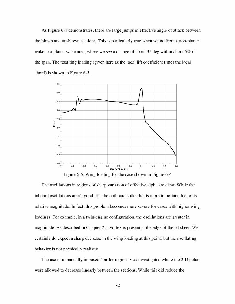
82
As Figure 6-4 demonstrates, there are large jumps in effective angle of attack between
the blown and un-blown sections. This is particularly true when we go from a non-planar
wake to a planar wake area, where we see a change of about 35 deg within about 5% of
the span. The resulting loading (given here as the local lift coefficient times the local
chord) is shown in Figure 6-5.
0.0
0.5
1.0
1.5
2.0
2.5
3.0
3.5
4.0
4.5
0.0 0.1 0.2 0.3 0.4 0.5 0.6 0.7 0.8 0.9 1.0
Eta (y/(b/2))
Cl x c
Figure 6-5: Wing loading for the case shown in Figure 6-4
The oscillations in regions of sharp variation of effective alpha are clear. While the
inboard oscillations aren’t good, it’s the outboard spike that is more important due to its
relative magnitude. In fact, this problem becomes more severe for cases with higher wing
loadings. For example, in a twin-engine configuration, the oscillations are greater in
magnitude. As described in Chapter 2, a vortex is present at the edge of the jet sheet. We
certainly do expect a sharp decrease in the wing loading at this point, but the oscillating
behavior is not physically realistic.
The use of a manually imposed “buffer region” was investigated where the 2-D polars
were allowed to decrease linearly between the sections. While this did reduce the

83
magnitude of these oscillations, it did not eliminate them. We hypothesize that the reason
for the oscillations is because the method is being forced to extrapolate the data well
beyond it’s input range. This fact, along with going from a non-planar wake to a planar
wake region, is responsible for the large spike experienced around η=0.70.
The significance of these oscillations lies primarily in the determination of induced
drag, CDi. While lift is also affected, the oscillations tend to cancel one another out
leaving the lift largely unchanged. Based on a Trefftz-plane derivation by Mason(15), the
induced drag of a wing can be given by:
€
Di =−ρ∞4π
dΓ(y1)dy
dΓ(y2)dy
ln y1 − y2( )dy1dy2−b2
b2∫−b
2
b2∫ (6-5)
We see that the induced drag is directly tied to the changes in the spanloading. Sharp
breaks or oscillations would mean that the induced drag becomes large. As will be shown
in the following chapter, for situations involving high wing loadings, this oscillation did
indeed dramatically increase the induced drag calculated.
The most obvious method to correct the excessive induced drag predictions is to
manually remove the oscillations from the spanloading. This procedure was investigated
for a representative case from Smith and Phelps(54) with δf = 20° and α = 25°. The high-
lift module output for this case was e = 0.364. Figure 6-6 shows the original output
spanload and the modified spanload with the oscillations removed:
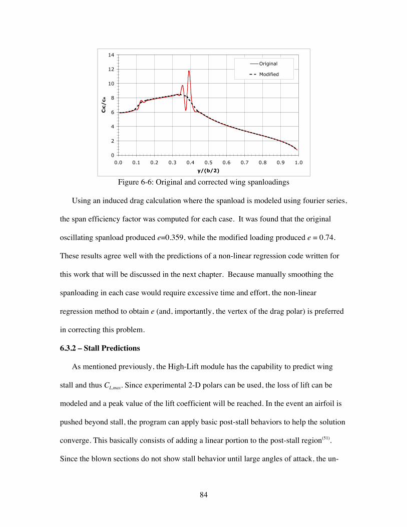
84
0
2
4
6
8
10
12
14
0.0 0.1 0.2 0.3 0.4 0.5 0.6 0.7 0.8 0.9 1.0
y/(b/2)
Clc/ca
Original
Modified
Figure 6-6: Original and corrected wing spanloadings
Using an induced drag calculation where the spanload is modeled using fourier series,
the span efficiency factor was computed for each case. It was found that the original
oscillating spanload produced e=0.359, while the modified loading produced e = 0.74.
These results agree well with the predictions of a non-linear regression code written for
this work that will be discussed in the next chapter. Because manually smoothing the
spanloading in each case would require excessive time and effort, the non-linear
regression method to obtain e (and, importantly, the vertex of the drag polar) is preferred
in correcting this problem.
6.3.2 – Stall Predictions
As mentioned previously, the High-Lift module has the capability to predict wing
stall and thus CL,max. Since experimental 2-D polars can be used, the loss of lift can be
modeled and a peak value of the lift coefficient will be reached. In the event an airfoil is
pushed beyond stall, the program can apply basic post-stall behaviors to help the solution
converge. This basically consists of adding a linear portion to the post-stall region(51).
Since the blown sections do not show stall behavior until large angles of attack, the un-

85
blown sections of the wing may stall without the aircraft experiencing the dramatic loss
of lift of a conventional design. The “stall” event for a USB aircraft configuration is more
appropriately viewed as the point at which the outboard control surfaces stall.
In the previous section it was demonstrated that wing sections adjacent to blown
sections experience a large upwash and are placed at a much larger effective angle of
attack. If viscous data is input, significant portions of the unblown section may be well
within the post-stall region. Numerically, if the post-stall corrections are not used within
the code, it will not converge to a solution. If post-stall corrections are used, the quality
of the output is highly dependent on the nature of the corrections. For this reason, only
unstalled 2-D polars were input, with the assumption being that sufficient leading edge
protection was present to delay stall behavior.
6.3.3 – Nacelle and Fuselage Effects
The High-Lift module was developed to accurately predict wing performance. As
such, only limited work was done on incorporating effects from other aircraft
components. There are currently some routines for estimating fuselage effects. They
consist of modifying the upwash field near the wing/fuselage junction. Since these
modifications have not been completely validated, this option was not used in any
calculations in the current work.
The engine nacelles are another component that can significantly contribute to the
aerodynamics. No force or pitching moment corrections are currently in place to address
the presence of the engine nacelles. The two main areas where this modeling would be
useful are in the additional friction drag they incur and the variations in CM,α they can
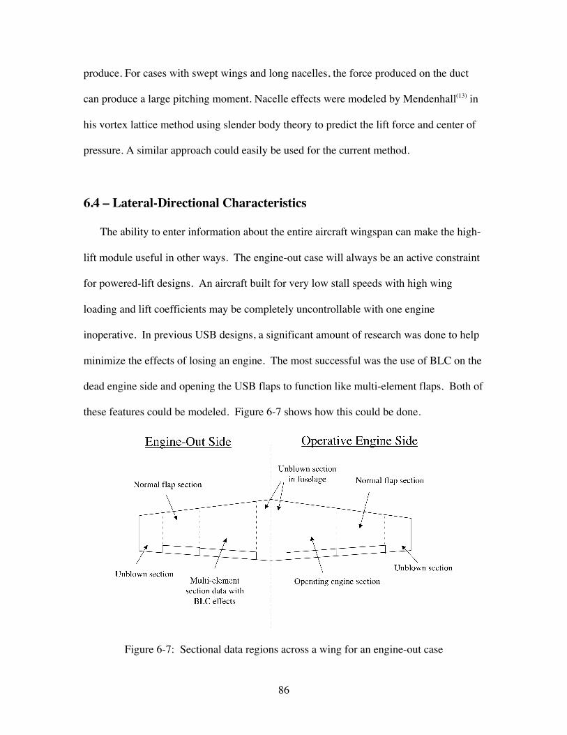
86
produce. For cases with swept wings and long nacelles, the force produced on the duct
can produce a large pitching moment. Nacelle effects were modeled by Mendenhall(13) in
his vortex lattice method using slender body theory to predict the lift force and center of
pressure. A similar approach could easily be used for the current method.
6.4 – Lateral-Directional Characteristics
The ability to enter information about the entire aircraft wingspan can make the high-
lift module useful in other ways. The engine-out case will always be an active constraint
for powered-lift designs. An aircraft built for very low stall speeds with high wing
loading and lift coefficients may be completely uncontrollable with one engine
inoperative. In previous USB designs, a significant amount of research was done to help
minimize the effects of losing an engine. The most successful was the use of BLC on the
dead engine side and opening the USB flaps to function like multi-element flaps. Both of
these features could be modeled. Figure 6-7 shows how this could be done.
Figure 6-7: Sectional data regions across a wing for an engine-out case

87
Once we know the CN, Cl, and CY contribution from the wing, the control authority to
maintain a given heading or orientation can be found from the equations of motion. This
process would work equally well for estimating the forces and moments we can generate
to assist in maneuvers. It should be noted that the ability of the current method to operate
in this aspect is crucial to facilitate the design decision process in the early design stages.

88
Chapter 7: Comparison with 3-D Experimental Results
This chapter presents direct comparisons of the new USB methodology with
experimental data. This data was obtained from a variety of sources, with the primary
sources being Technical Notes published by NASA. The wind tunnel models include a
wide range of scales and configurations. Because of this, individual cases had to be
modeled differently to approximate the flap system and propulsion conditions
appropriately. Any corrections or adjustments made to capture other influences will also
be discussed. It was found that the current method typically approximated the magnitude
of aerodynamic coefficients within 10% and also captured derivative information (CLα,
Cmα) very well over a broad range of inputs.
We also present a short comparison of the new USB methodology with an
engineering method produced by Mendenhall and Spangler(13). This method is based on a
non-linear vortex lattice method for USB aircraft. The authors also performed
comparisons with NASA Technical Note data sets. It was found that the current
methodology compares very well with the non-linear VLM.
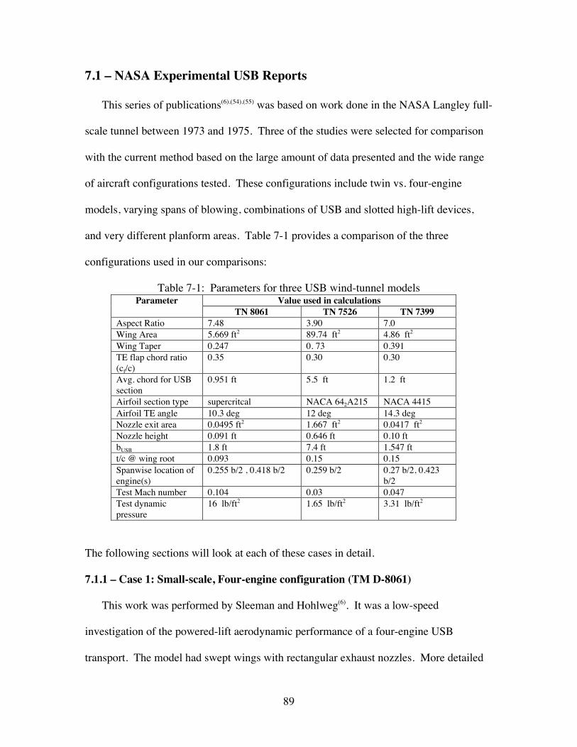
89
7.1 – NASA Experimental USB Reports
This series of publications(6),(54),(55) was based on work done in the NASA Langley full-
scale tunnel between 1973 and 1975. Three of the studies were selected for comparison
with the current method based on the large amount of data presented and the wide range
of aircraft configurations tested. These configurations include twin vs. four-engine
models, varying spans of blowing, combinations of USB and slotted high-lift devices,
and very different planform areas. Table 7-1 provides a comparison of the three
configurations used in our comparisons:
Table 7-1: Parameters for three USB wind-tunnel modelsValue used in calculationsParameter
TN 8061 TN 7526 TN 7399Aspect Ratio 7.48 3.90 7.0Wing Area 5.669 ft2 89.74 ft2 4.86 ft2
Wing Taper 0.247 0. 73 0.391TE flap chord ratio(cf/c)
0.35 0.30 0.30
Avg. chord for USBsection
0.951 ft 5.5 ft 1.2 ft
Airfoil section type supercritcal NACA 642A215 NACA 4415Airfoil TE angle 10.3 deg 12 deg 14.3 degNozzle exit area 0.0495 ft2 1.667 ft2 0.0417 ft2
Nozzle height 0.091 ft 0.646 ft 0.10 ftbUSB 1.8 ft 7.4 ft 1.547 ftt/c @ wing root 0.093 0.15 0.15Spanwise location ofengine(s)
0.255 b/2 , 0.418 b/2 0.259 b/2 0.27 b/2, 0.423b/2
Test Mach number 0.104 0.03 0.047Test dynamicpressure
16 lb/ft2 1.65 lb/ft2 3.31 lb/ft2
The following sections will look at each of these cases in detail.
7.1.1 – Case 1: Small-scale, Four-engine configuration (TM D-8061)
This work was performed by Sleeman and Hohlweg(6). It was a low-speed
investigation of the powered-lift aerodynamic performance of a four-engine USB
transport. The model had swept wings with rectangular exhaust nozzles. More detailed
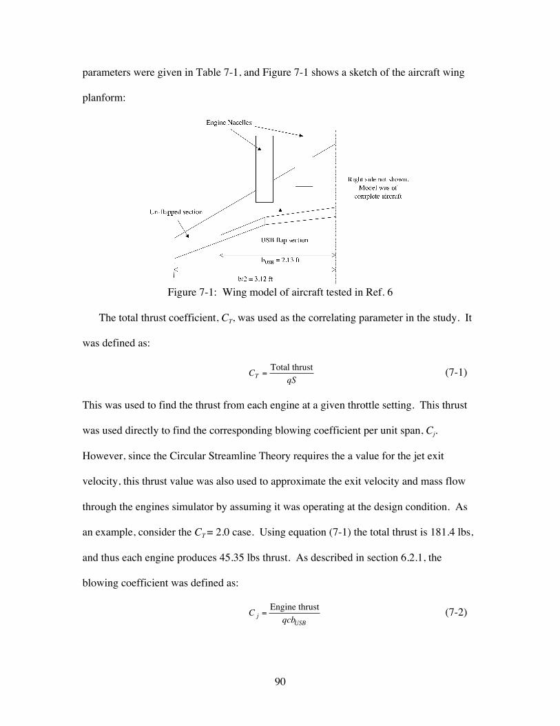
90
parameters were given in Table 7-1, and Figure 7-1 shows a sketch of the aircraft wing
planform:
Figure 7-1: Wing model of aircraft tested in Ref. 6
The total thrust coefficient, CT, was used as the correlating parameter in the study. It
was defined as:
€
CT =Total thrust
qS(7-1)
This was used to find the thrust from each engine at a given throttle setting. This thrust
was used directly to find the corresponding blowing coefficient per unit span, Cj.
However, since the Circular Streamline Theory requires the a value for the jet exit
velocity, this thrust value was also used to approximate the exit velocity and mass flow
through the engines simulator by assuming it was operating at the design condition. As
an example, consider the CT = 2.0 case. Using equation (7-1) the total thrust is 181.4 lbs,
and thus each engine produces 45.35 lbs thrust. As described in section 6.2.1, the
blowing coefficient was defined as:
€
C j =Engine thrust
qcbUSB(7-2)
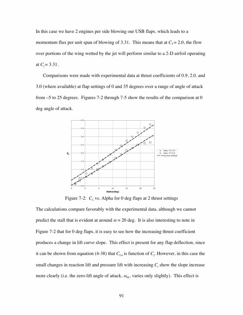
91
In this case we have 2 engines per side blowing our USB flaps, which leads to a
momentum flux per unit span of blowing of 3.31. This means that at CT = 2.0, the flow
over portions of the wing wetted by the jet will perform similar to a 2-D airfoil operating
at Cj = 3.31.
Comparisons were made with experimental data at thrust coefficients of 0.9, 2.0, and
3.0 (where available) at flap settings of 0 and 35 degrees over a range of angle of attack
from –5 to 25 degrees. Figures 7-2 through 7-5 show the results of the comparison at 0
deg angle of attack.
0.0
0.5
1.0
1.5
2.0
2.5
3.0
3.5
4.0
-5 0 5 10 15 20 25
Alpha(deg)
CLData, CT=2.0Data, CT=0.9Current method
Figure 7-2: CL vs. Alpha for 0 deg flaps at 2 thrust settings
The calculations compare favorably with the experimental data, although we cannot
predict the stall that is evident at around α = 20 deg. It is also interesting to note in
Figure 7-2 that for 0 deg flaps, it is easy to see how the increasing thrust coefficient
produces a change in lift curve slope. This effect is present for any flap deflection, since
it can be shown from equation (4-38) that CLα is function of Cj. However, in this case the
small changes in reaction lift and pressure lift with increasing Cj show the slope increase
more clearly (i.e. the zero-lift angle of attack, α0L, varies only slightly). This effect is
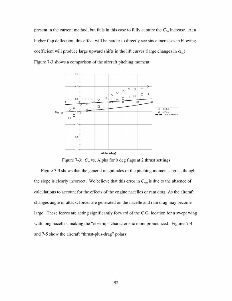
92
present in the current method, but fails in this case to fully capture the CLα increase. At a
higher flap deflection, this effect will be harder to directly see since increases in blowing
coefficient will produce large upward shifts in the lift curves (large changes in α0L).
Figure 7-3 shows a comparison of the aircraft pitching moment:
-2.0
-1.5
-1.0
-0.5
0.0
0.5
1.0
-5 0 5 10 15 20 25
Alpha (deg)
Cm, CG
Cj=0.9Cj=2.0Current method
Figure 7-3: Cm vs. Alpha for 0 deg flaps at 2 thrust settings
Figure 7-3 shows that the general magnitudes of the pitching moments agree, though
the slope is clearly incorrect. We believe that this error in Cmα is due to the absence of
calculations to account for the effects of the engine nacelles or ram drag. As the aircraft
changes angle of attack, forces are generated on the nacelle and ram drag may become
large. These forces are acting significantly forward of the C.G. location for a swept wing
with long nacelles, making the “nose-up” characteristic more pronounced. Figures 7-4
and 7-5 show the aircraft “thrust-plus-drag” polars:
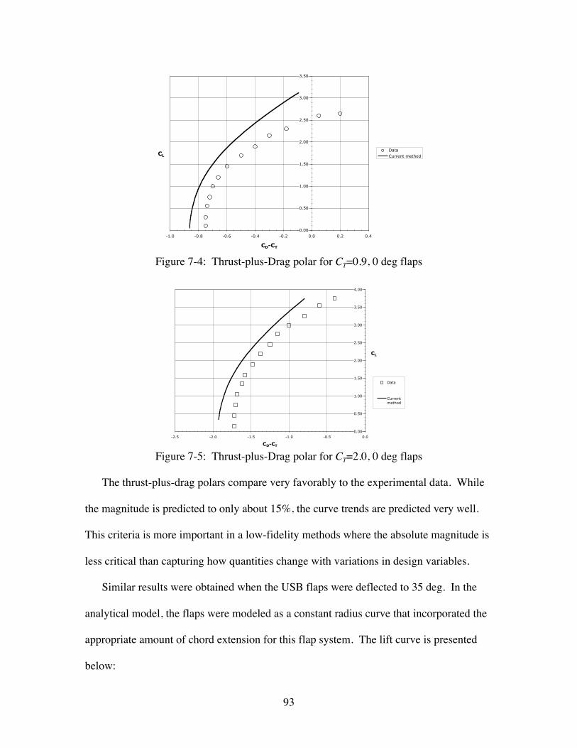
93
0.00
0.50
1.00
1.50
2.00
2.50
3.00
3.50
-1.0 -0.8 -0.6 -0.4 -0.2 0.0 0.2 0.4
CD-CT
CLDataCurrent method
Figure 7-4: Thrust-plus-Drag polar for CT=0.9, 0 deg flaps
0.00
0.50
1.00
1.50
2.00
2.50
3.00
3.50
4.00
-2.5 -2.0 -1.5 -1.0 -0.5 0.0
CD-CT
CL
Data
Currentmethod
Figure 7-5: Thrust-plus-Drag polar for CT=2.0, 0 deg flaps
The thrust-plus-drag polars compare very favorably to the experimental data. While
the magnitude is predicted to only about 15%, the curve trends are predicted very well.
This criteria is more important in a low-fidelity methods where the absolute magnitude is
less critical than capturing how quantities change with variations in design variables.
Similar results were obtained when the USB flaps were deflected to 35 deg. In the
analytical model, the flaps were modeled as a constant radius curve that incorporated the
appropriate amount of chord extension for this flap system. The lift curve is presented
below:
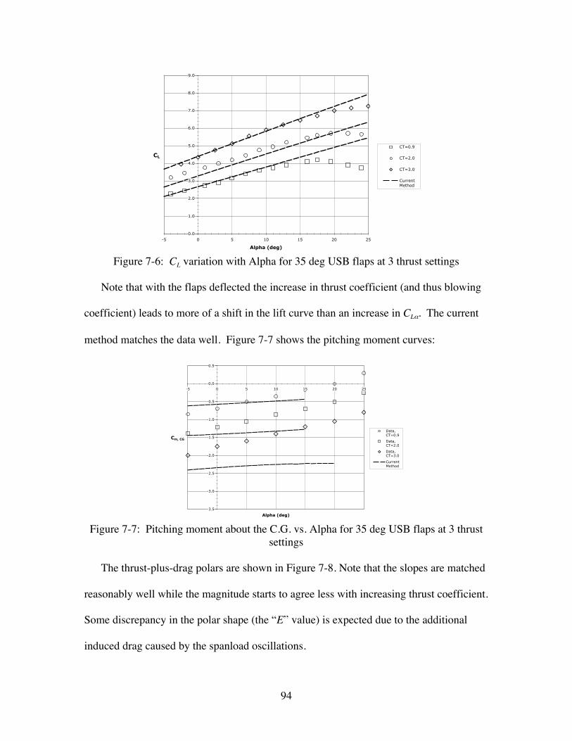
94
0.0
1.0
2.0
3.0
4.0
5.0
6.0
7.0
8.0
9.0
-5 0 5 10 15 20 25
Alpha (deg)
CL
CT=0.9
CT=2.0
CT=3.0
CurrentMethod
Figure 7-6: CL variation with Alpha for 35 deg USB flaps at 3 thrust settings
Note that with the flaps deflected the increase in thrust coefficient (and thus blowing
coefficient) leads to more of a shift in the lift curve than an increase in CLα. The current
method matches the data well. Figure 7-7 shows the pitching moment curves:
-3.5
-3.0
-2.5
-2.0
-1.5
-1.0
-0.5
0.0
0.5
-5 0 5 10 15 20 25
Alpha (deg)
Cm, CG
Data,CT=0.9
Data,CT=2.0
Data,CT=3.0
CurrentMethod
Figure 7-7: Pitching moment about the C.G. vs. Alpha for 35 deg USB flaps at 3 thrustsettings
The thrust-plus-drag polars are shown in Figure 7-8. Note that the slopes are matched
reasonably well while the magnitude starts to agree less with increasing thrust coefficient.
Some discrepancy in the polar shape (the “E” value) is expected due to the additional
induced drag caused by the spanload oscillations.
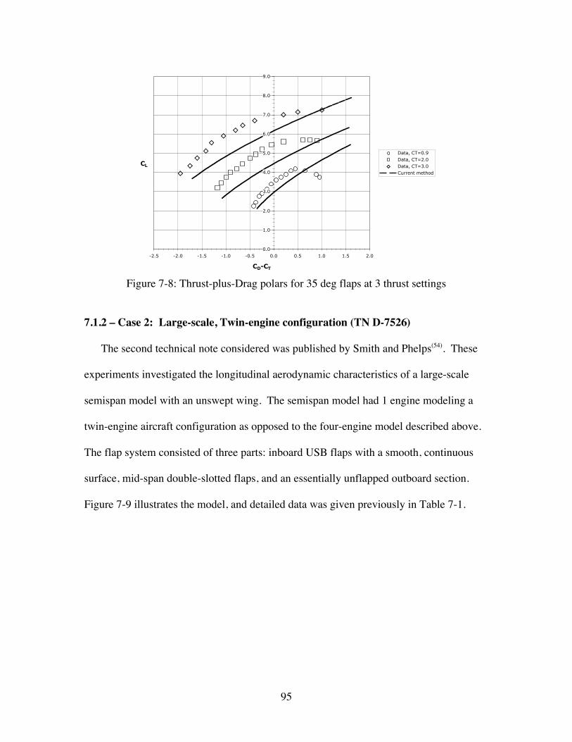
95
0.0
1.0
2.0
3.0
4.0
5.0
6.0
7.0
8.0
9.0
-2.5 -2.0 -1.5 -1.0 -0.5 0.0 0.5 1.0 1.5 2.0
CD-CT
CL
Data, CT=0.9Data, CT=2.0Data, CT=3.0Current method
Figure 7-8: Thrust-plus-Drag polars for 35 deg flaps at 3 thrust settings
7.1.2 – Case 2: Large-scale, Twin-engine configuration (TN D-7526)
The second technical note considered was published by Smith and Phelps(54). These
experiments investigated the longitudinal aerodynamic characteristics of a large-scale
semispan model with an unswept wing. The semispan model had 1 engine modeling a
twin-engine aircraft configuration as opposed to the four-engine model described above.
The flap system consisted of three parts: inboard USB flaps with a smooth, continuous
surface, mid-span double-slotted flaps, and an essentially unflapped outboard section.
Figure 7-9 illustrates the model, and detailed data was given previously in Table 7-1.
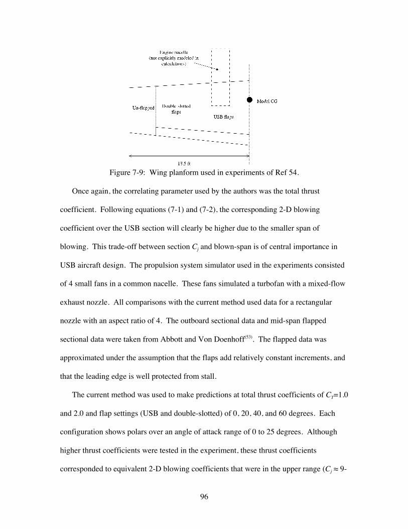
96
Figure 7-9: Wing planform used in experiments of Ref 54.
Once again, the correlating parameter used by the authors was the total thrust
coefficient. Following equations (7-1) and (7-2), the corresponding 2-D blowing
coefficient over the USB section will clearly be higher due to the smaller span of
blowing. This trade-off between section Cj and blown-span is of central importance in
USB aircraft design. The propulsion system simulator used in the experiments consisted
of 4 small fans in a common nacelle. These fans simulated a turbofan with a mixed-flow
exhaust nozzle. All comparisons with the current method used data for a rectangular
nozzle with an aspect ratio of 4. The outboard sectional data and mid-span flapped
sectional data were taken from Abbott and Von Doenhoff(53). The flapped data was
approximated under the assumption that the flaps add relatively constant increments, and
that the leading edge is well protected from stall.
The current method was used to make predictions at total thrust coefficients of CT=1.0
and 2.0 and flap settings (USB and double-slotted) of 0, 20, 40, and 60 degrees. Each
configuration shows polars over an angle of attack range of 0 to 25 degrees. Although
higher thrust coefficients were tested in the experiment, these thrust coefficients
corresponded to equivalent 2-D blowing coefficients that were in the upper range (Cj ≈ 9-
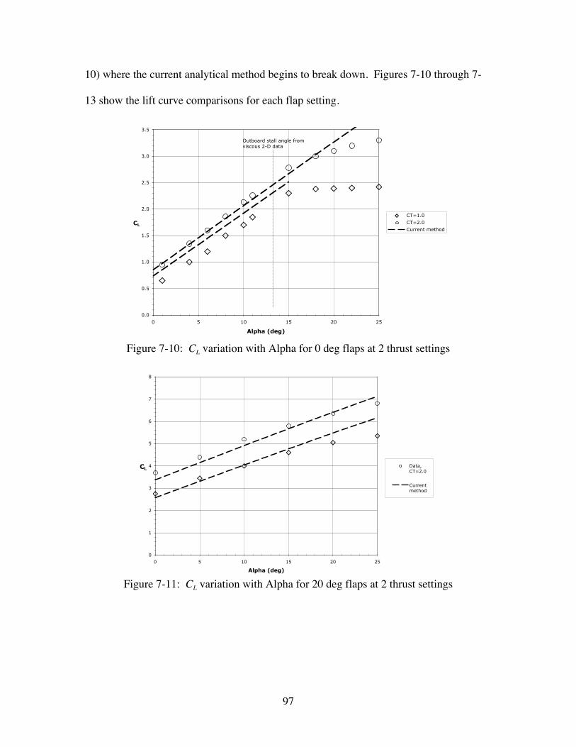
97
10) where the current analytical method begins to break down. Figures 7-10 through 7-
13 show the lift curve comparisons for each flap setting.
0.0
0.5
1.0
1.5
2.0
2.5
3.0
3.5
0 5 10 15 20 25
Alpha (deg)
CL
CT=1.0CT=2.0Current method
Outboard stall angle from viscous 2-D data
Figure 7-10: CL variation with Alpha for 0 deg flaps at 2 thrust settings
0
1
2
3
4
5
6
7
8
0 5 10 15 20 25
Alpha (deg)
CLData,CT=2.0
Currentmethod
Figure 7-11: CL variation with Alpha for 20 deg flaps at 2 thrust settings
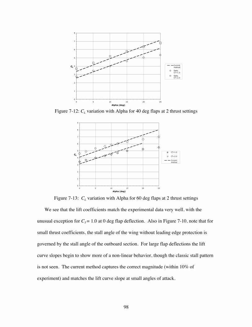
98
0
1
2
3
4
5
6
7
8
0 5 10 15 20 25
Alpha (deg)
CLCurrentmethod
Data,CT=1.0
Data,CT=2.0
Figure 7-12: CL variation with Alpha for 40 deg flaps at 2 thrust settings
0
1
2
3
4
5
6
7
8
9
0 5 10 15 20 25
Alpha (deg)
CL
CT=1.0
CT=2.0
Currentmethod
Figure 7-13: CL variation with Alpha for 60 deg flaps at 2 thrust settings
We see that the lift coefficients match the experimental data very well, with the
unusual exception for CT = 1.0 at 0 deg flap deflection. Also in Figure 7-10, note that for
small thrust coefficients, the stall angle of the wing without leading edge protection is
governed by the stall angle of the outboard section. For large flap deflections the lift
curve slopes begin to show more of a non-linear behavior, though the classic stall pattern
is not seen. The current method captures the correct magnitude (within 10% of
experiment) and matches the lift curve slope at small angles of attack.

99
Next, examine the drag coefficient predictions with experiment. As described in
section 6.3, the high-lift module encounters numerical problems when dealing with rapid
changes in the sectional properties across the span, and a twin-engine configuration will
have such changes. To counter the additional induced drag that is predicted, a small
study was done on the experimental data to determine the general values of the span
efficiency factor, e. The parabolic form of the drag equation is:
€
CD = CD,M +1
πARe
CL −CL,M( )2 (7-3)
where AR is the aspect ratio and CD,M and CL,M are the drag and lift coefficients at the
parabola vertex.
Using methods described by Recktenwald(56), a short non-linear regression program
was written in MATLAB as part of the current work. Experimental data sets were then
input and the span efficiency factor determined. It was found that the magnitude of e
varied between about 0.50 and 0.70 with most cases being around 0.63 for the
experimental cases. There also appeared to be an increase in the efficiency factor with
increasing blowing coefficient. This effect was also described by Whitten(57), who says
regarding the drag with increasing power setting, “…an improvement in polar shape is
obtained along with an increase in minimum drag”. The efficiency factors output from
the high-lift module were typically around e = 0.35 and varied very little with power
setting.
Using the non-linear regression program, values of e, CD,M and CL,M were obtained for
the output drag polars, and then equation (7-3) was used with an improved value for e to
basically “reconstruct” a polar. The resulting drag polars had a more appropriate shape
and much better agreement in magnitude. An example of this change is shown in Figure
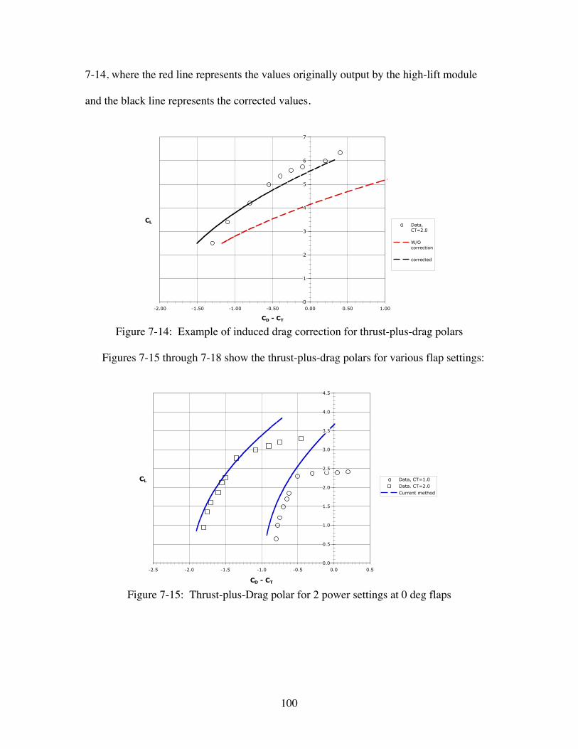
100
7-14, where the red line represents the values originally output by the high-lift module
and the black line represents the corrected values.
0
1
2
3
4
5
6
7
-2.00 -1.50 -1.00 -0.50 0.00 0.50 1.00
CD - CT
CLData,CT=2.0
W/Ocorrection
corrected
Figure 7-14: Example of induced drag correction for thrust-plus-drag polars
Figures 7-15 through 7-18 show the thrust-plus-drag polars for various flap settings:
0.0
0.5
1.0
1.5
2.0
2.5
3.0
3.5
4.0
4.5
-2.5 -2.0 -1.5 -1.0 -0.5 0.0 0.5
CD - CT
CL Data, CT=1.0Data. CT=2.0Current method
Figure 7-15: Thrust-plus-Drag polar for 2 power settings at 0 deg flaps
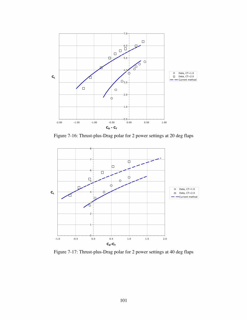
101
0.0
1.0
2.0
3.0
4.0
5.0
6.0
7.0
-2.00 -1.50 -1.00 -0.50 0.00 0.50 1.00
CD - CT
CL
Data, CT=1.0Data, CT=2.0Current method
Figure 7-16: Thrust-plus-Drag polar for 2 power settings at 20 deg flaps
0
1
2
3
4
5
6
7
8
-1.0 -0.5 0.0 0.5 1.0 1.5 2.0
CD-CT
CLData, CT=1.0
Data, CT=2.0
Current method
Figure 7-17: Thrust-plus-Drag polar for 2 power settings at 40 deg flaps
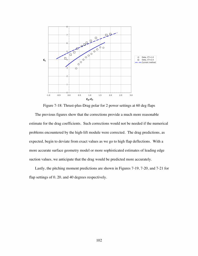
102
0
1
2
3
4
5
6
7
8
-1.0 -0.5 0.0 0.5 1.0 1.5 2.0 2.5 3.0
CD-CT
CLData, CT=1.0Data, CT=2.0Current method
Figure 7-18: Thrust-plus-Drag polar for 2 power settings at 60 deg flaps
The previous figures show that the corrections provide a much more reasonable
estimate for the drag coefficients. Such corrections would not be needed if the numerical
problems encountered by the high-lift module were corrected. The drag predictions, as
expected, begin to deviate from exact values as we go to high flap deflections. With a
more accurate surface geometry model or more sophisticated estimates of leading edge
suction values, we anticipate that the drag would be predicted more accurately.
Lastly, the pitching moment predictions are shown in Figures 7-19, 7-20, and 7-21 for
flap settings of 0, 20, and 40 degrees respectively.
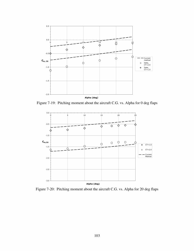
103
-2.0
-1.5
-1.0
-0.5
0.0
0.5
0 5 10 15 20 25
Alpha (deg)
Cm, CG
Currentmethod
Data,CT=2.0
Data,CT=1.0
Figure 7-19: Pitching moment about the aircraft C.G. vs. Alpha for 0 deg flaps
-3.0
-2.5
-2.0
-1.5
-1.0
-0.5
0.00 5 10 15 20 25
Alpha (deg)
Cm,CG
CT=1.0
CT=2.0
CurrentMethod
Figure 7-20: Pitching moment about the aircraft C.G. vs. Alpha for 20 deg flaps
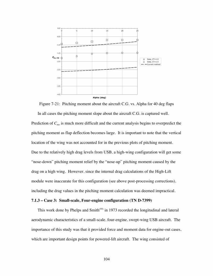
104
-4.0
-3.5
-3.0
-2.5
-2.0
-1.5
-1.0
-0.5
0.0
0 5 10 15 20 25
Alpha (deg)
Cm, CGData, CT=1.0
Data, CT=1.0
Current method
Figure 7-21: Pitching moment about the aircraft C.G. vs. Alpha for 40 deg flaps
In all cases the pitching moment slope about the aircraft C.G. is captured well.
Prediction of Cmo is much more difficult and the current analysis begins to overpredict the
pitching moment as flap deflection becomes large. It is important to note that the vertical
location of the wing was not accounted for in the previous plots of pitching moment.
Due to the relatively high drag levels from USB, a high-wing configuration will get some
“nose-down” pitching moment relief by the “nose-up” pitching moment caused by the
drag on a high wing. However, since the internal drag calculations of the High-Lift
module were inaccurate for this configuration (see above post-processing corrections),
including the drag values in the pitching moment calculation was deemed impractical.
7.1.3 – Case 3: Small-scale, Four-engine configuration (TN D-7399)
This work done by Phelps and Smith(55) in 1973 recorded the longitudinal and lateral
aerodynamic characteristics of a small-scale, four-engine, swept-wing USB aircraft. The
importance of this study was that it provided force and moment data for engine-out cases,
which are important design points for powered-lift aircraft. The wing consisted of
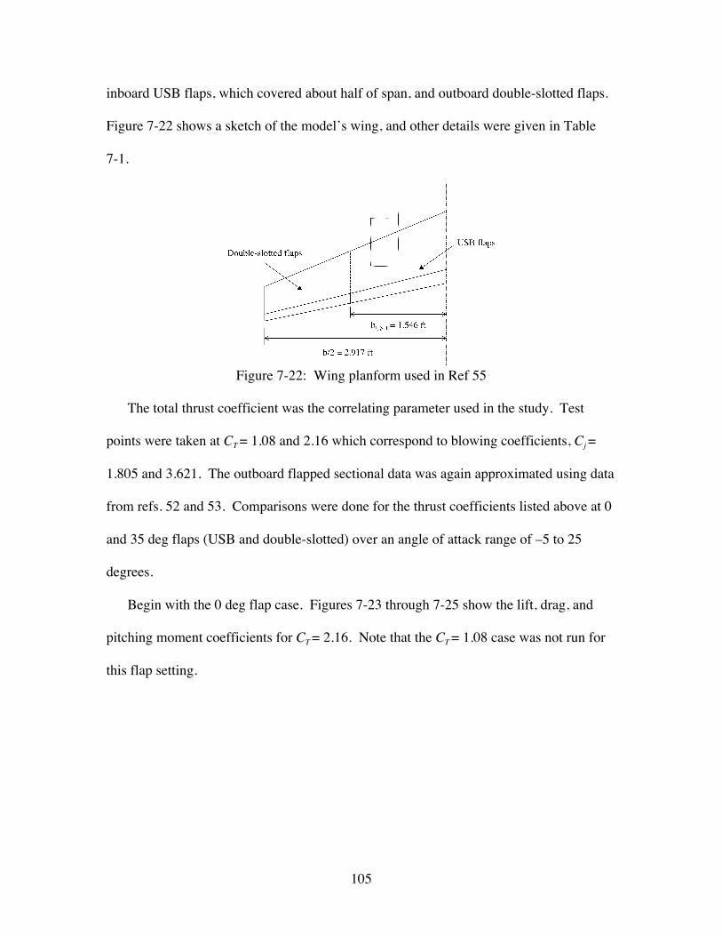
105
inboard USB flaps, which covered about half of span, and outboard double-slotted flaps.
Figure 7-22 shows a sketch of the model’s wing, and other details were given in Table
7-1.
Figure 7-22: Wing planform used in Ref 55
The total thrust coefficient was the correlating parameter used in the study. Test
points were taken at CT = 1.08 and 2.16 which correspond to blowing coefficients, Cj =
1.805 and 3.621. The outboard flapped sectional data was again approximated using data
from refs. 52 and 53. Comparisons were done for the thrust coefficients listed above at 0
and 35 deg flaps (USB and double-slotted) over an angle of attack range of –5 to 25
degrees.
Begin with the 0 deg flap case. Figures 7-23 through 7-25 show the lift, drag, and
pitching moment coefficients for CT = 2.16. Note that the CT = 1.08 case was not run for
this flap setting.
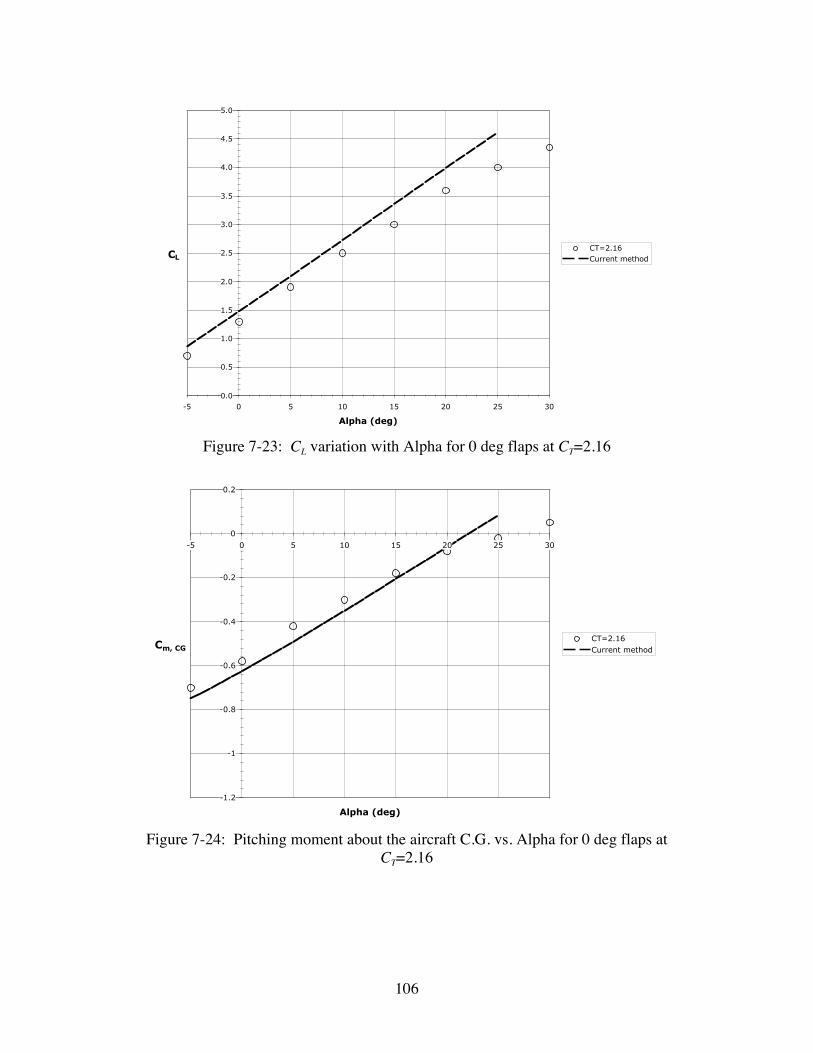
106
0.0
0.5
1.0
1.5
2.0
2.5
3.0
3.5
4.0
4.5
5.0
-5 0 5 10 15 20 25 30
Alpha (deg)
CLCT=2.16Current method
Figure 7-23: CL variation with Alpha for 0 deg flaps at CT=2.16
-1.2
-1
-0.8
-0.6
-0.4
-0.2
0
0.2
-5 0 5 10 15 20 25 30
Alpha (deg)
Cm, CGCT=2.16Current method
Figure 7-24: Pitching moment about the aircraft C.G. vs. Alpha for 0 deg flaps atCT=2.16
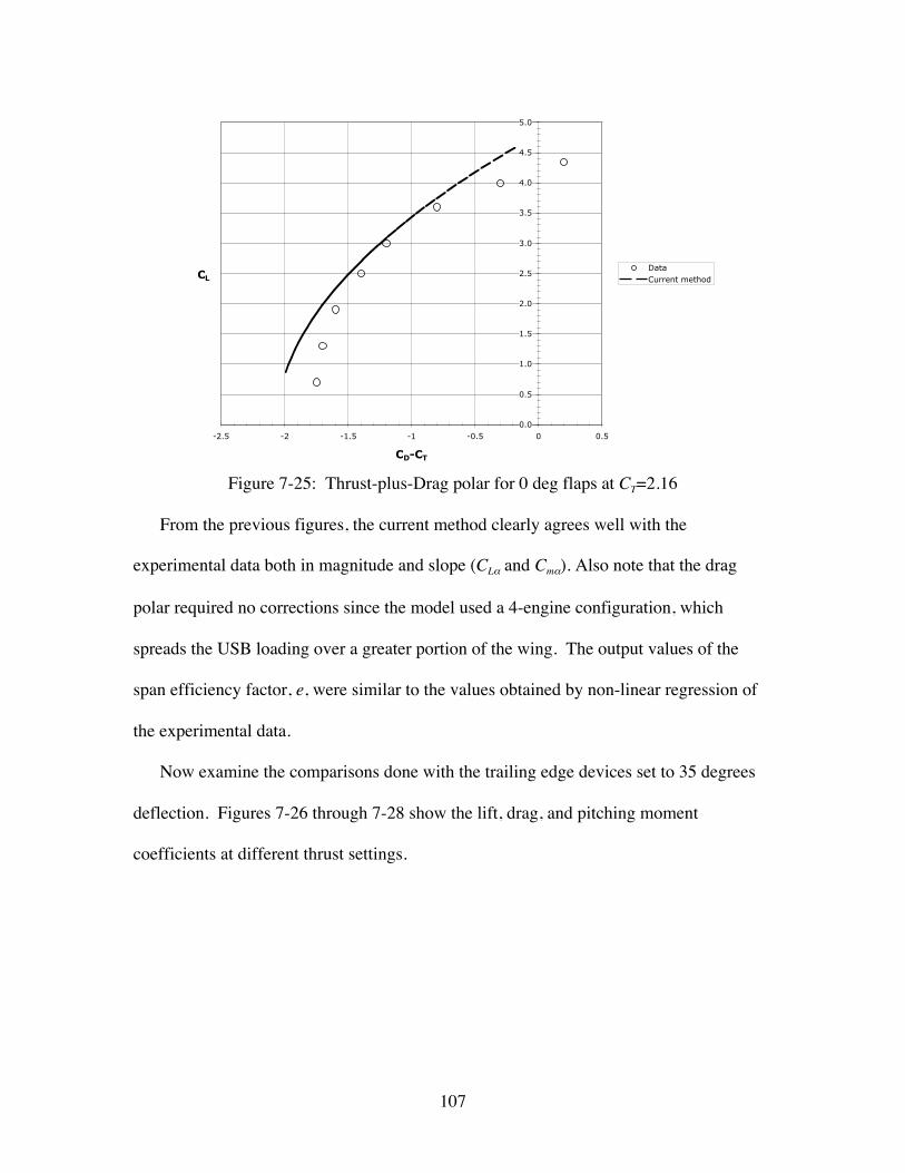
107
0.0
0.5
1.0
1.5
2.0
2.5
3.0
3.5
4.0
4.5
5.0
-2.5 -2 -1.5 -1 -0.5 0 0.5
CD-CT
CLDataCurrent method
Figure 7-25: Thrust-plus-Drag polar for 0 deg flaps at CT=2.16
From the previous figures, the current method clearly agrees well with the
experimental data both in magnitude and slope (CLα and Cmα). Also note that the drag
polar required no corrections since the model used a 4-engine configuration, which
spreads the USB loading over a greater portion of the wing. The output values of the
span efficiency factor, e, were similar to the values obtained by non-linear regression of
the experimental data.
Now examine the comparisons done with the trailing edge devices set to 35 degrees
deflection. Figures 7-26 through 7-28 show the lift, drag, and pitching moment
coefficients at different thrust settings.
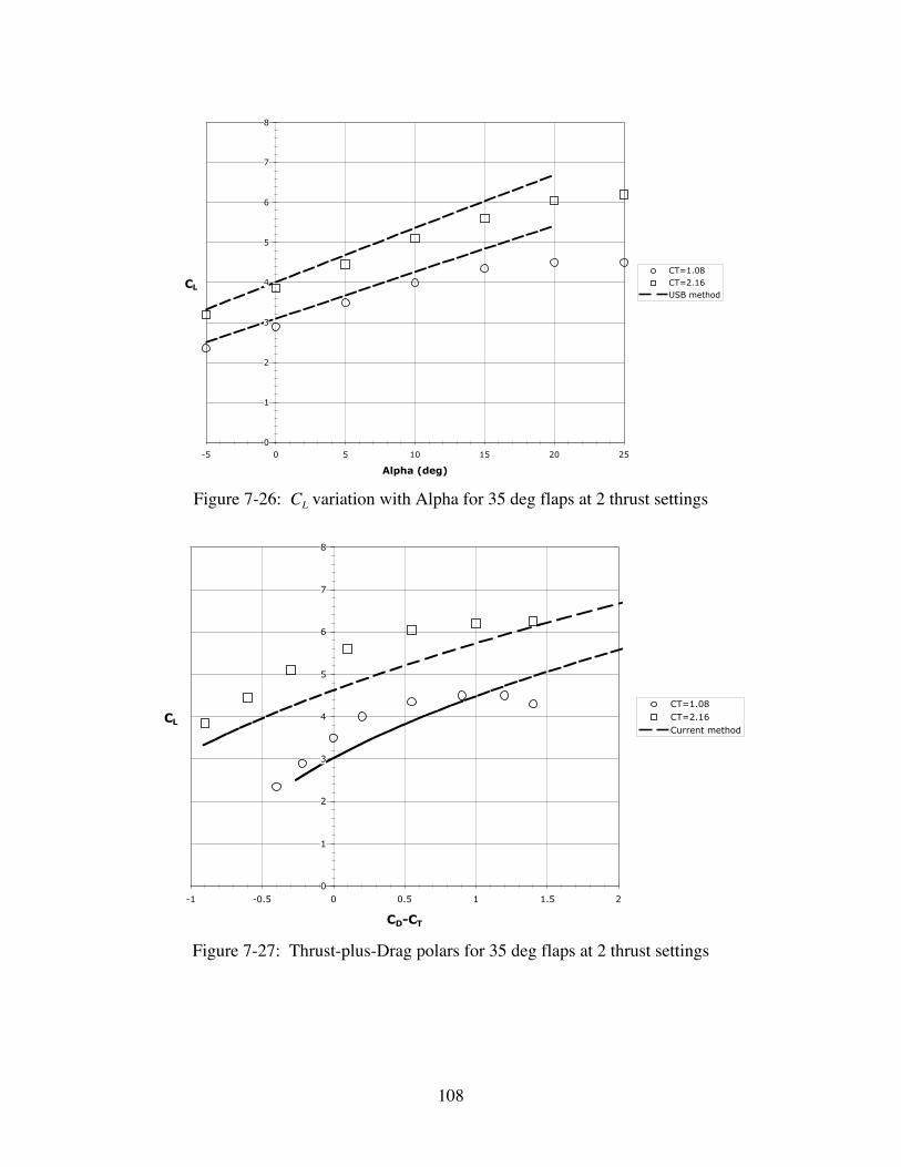
108
0
1
2
3
4
5
6
7
8
-5 0 5 10 15 20 25
Alpha (deg)
CL
CT=1.08CT=2.16USB method
Figure 7-26: CL variation with Alpha for 35 deg flaps at 2 thrust settings
0
1
2
3
4
5
6
7
8
-1 -0.5 0 0.5 1 1.5 2
CD-CT
CLCT=1.08CT=2.16Current method
Figure 7-27: Thrust-plus-Drag polars for 35 deg flaps at 2 thrust settings
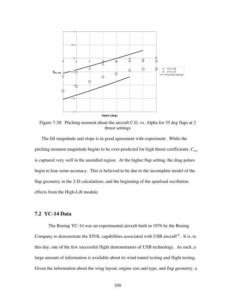
109
-2
-1.5
-1
-0.5
0
0.5
1
-5 0 5 10 15 20 25 30
Alpha (deg)
Cm, CG
CT=1.08CT=2.16Current method
Figure 7-28: Pitching moment about the aircraft C.G. vs. Alpha for 35 deg flaps at 2thrust settings
The lift magnitude and slope is in good agreement with experiment. While the
pitching moment magnitude begins to be over-predicted for high thrust coefficients, Cmα
is captured very well in the unstalled region. At the higher flap setting, the drag polars
begin to lose some accuracy. This is believed to be due to the incomplete model of the
flap geometry in the 2-D calculations, and the beginning of the spanload oscillation
effects from the High-Lift module.
7.2 YC-14 Data
The Boeing YC-14 was an experimental aircraft built in 1976 by the Boeing
Company to demonstrate the STOL capabilities associated with USB aircraft(5). It is, to
this day, one of the few successful flight demonstrators of USB technology. As such, a
large amount of information is available about its wind tunnel testing and flight testing.
Given the information about the wing layout, engine size and type, and flap geometry, a
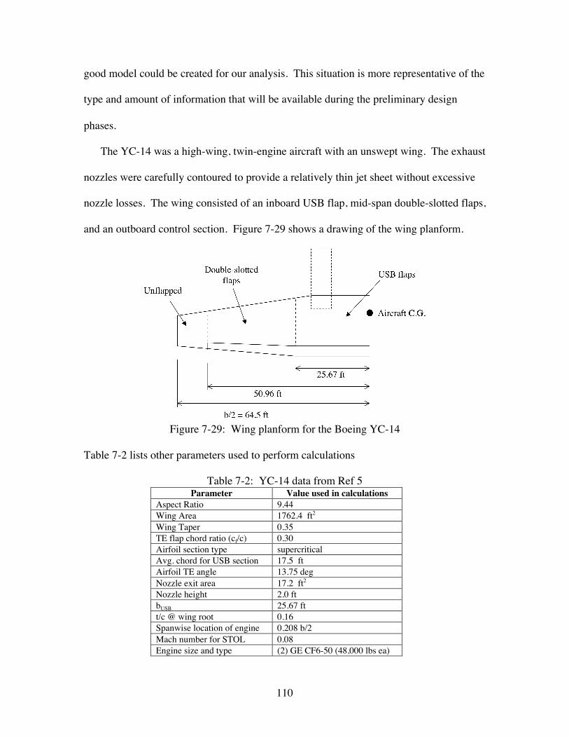
110
good model could be created for our analysis. This situation is more representative of the
type and amount of information that will be available during the preliminary design
phases.
The YC-14 was a high-wing, twin-engine aircraft with an unswept wing. The exhaust
nozzles were carefully contoured to provide a relatively thin jet sheet without excessive
nozzle losses. The wing consisted of an inboard USB flap, mid-span double-slotted flaps,
and an outboard control section. Figure 7-29 shows a drawing of the wing planform.
Figure 7-29: Wing planform for the Boeing YC-14
Table 7-2 lists other parameters used to perform calculations
Table 7-2: YC-14 data from Ref 5Parameter Value used in calculations
Aspect Ratio 9.44Wing Area 1762.4 ft2
Wing Taper 0.35TE flap chord ratio (cf/c) 0.30Airfoil section type supercriticalAvg. chord for USB section 17.5 ftAirfoil TE angle 13.75 degNozzle exit area 17.2 ft2
Nozzle height 2.0 ftbUSB 25.67 ftt/c @ wing root 0.16Spanwise location of engine 0.208 b/2Mach number for STOL 0.08Engine size and type (2) GE CF6-50 (48,000 lbs ea)
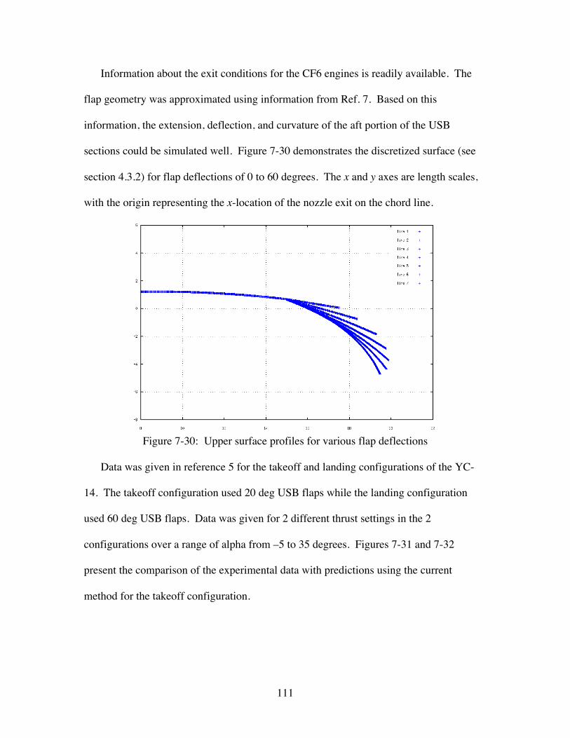
111
Information about the exit conditions for the CF6 engines is readily available. The
flap geometry was approximated using information from Ref. 7. Based on this
information, the extension, deflection, and curvature of the aft portion of the USB
sections could be simulated well. Figure 7-30 demonstrates the discretized surface (see
section 4.3.2) for flap deflections of 0 to 60 degrees. The x and y axes are length scales,
with the origin representing the x-location of the nozzle exit on the chord line.
Figure 7-30: Upper surface profiles for various flap deflections
Data was given in reference 5 for the takeoff and landing configurations of the YC-
14. The takeoff configuration used 20 deg USB flaps while the landing configuration
used 60 deg USB flaps. Data was given for 2 different thrust settings in the 2
configurations over a range of alpha from –5 to 35 degrees. Figures 7-31 and 7-32
present the comparison of the experimental data with predictions using the current
method for the takeoff configuration.
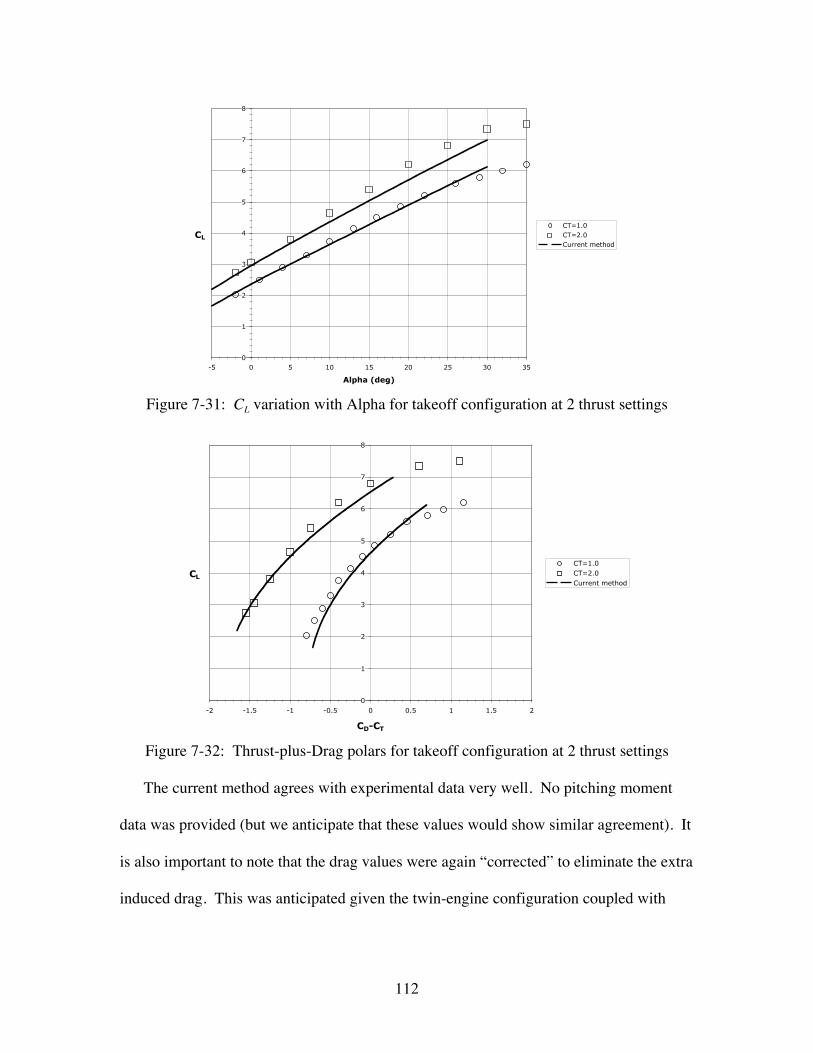
112
0
1
2
3
4
5
6
7
8
-5 0 5 10 15 20 25 30 35
Alpha (deg)
CL
CT=1.0CT=2.0Current method
Figure 7-31: CL variation with Alpha for takeoff configuration at 2 thrust settings
0
1
2
3
4
5
6
7
8
-2 -1.5 -1 -0.5 0 0.5 1 1.5 2
CD-CT
CLCT=1.0CT=2.0Current method
Figure 7-32: Thrust-plus-Drag polars for takeoff configuration at 2 thrust settings
The current method agrees with experimental data very well. No pitching moment
data was provided (but we anticipate that these values would show similar agreement). It
is also important to note that the drag values were again “corrected” to eliminate the extra
induced drag. This was anticipated given the twin-engine configuration coupled with
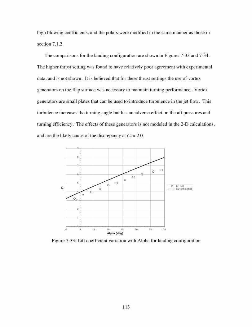
113
high blowing coefficients, and the polars were modified in the same manner as those in
section 7.1.2.
The comparisons for the landing configuration are shown in Figures 7-33 and 7-34.
The higher thrust setting was found to have relatively poor agreement with experimental
data, and is not shown. It is believed that for these thrust settings the use of vortex
generators on the flap surface was necessary to maintain turning performance. Vortex
generators are small plates that can be used to introduce turbulence in the jet flow. This
turbulence increases the turning angle but has an adverse effect on the aft pressures and
turning efficiency. The effects of these generators is not modeled in the 2-D calculations,
and are the likely cause of the discrepancy at CT = 2.0.
0
1
2
3
4
5
6
7
8
9
-5 0 5 10 15 20 25 30
Alpha (deg)
CLCT=1.0Current method
Figure 7-33: Lift coefficient variation with Alpha for landing configuration
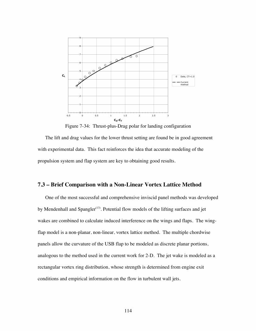
114
0
1
2
3
4
5
6
7
8
9
-0.5 0 0.5 1 1.5 2 2.5 3
CD-CT
CL Data, CT=1.0
Currentmethod
Figure 7-34: Thrust-plus-Drag polar for landing configuration
The lift and drag values for the lower thrust setting are found be in good agreement
with experimental data. This fact reinforces the idea that accurate modeling of the
propulsion system and flap system are key to obtaining good results.
7.3 – Brief Comparison with a Non-Linear Vortex Lattice Method
One of the most successful and comprehensive inviscid panel methods was developed
by Mendenhall and Spangler(13). Potential flow models of the lifting surfaces and jet
wakes are combined to calculate induced interference on the wings and flaps. The wing-
flap model is a non-planar, non-linear, vortex lattice method. The multiple chordwise
panels allow the curvature of the USB flap to be modeled as discrete planar portions,
analogous to the method used in the current work for 2-D. The jet wake is modeled as a
rectangular vortex ring distribution, whose strength is determined from engine exit
conditions and empirical information on the flow in turbulent wall jets.

115
The VLM method can calculate longitudinal effects in incompressible flow. It can
handle any kind of wing geometry including dihedral, sweep, twist, and camber. The jet
wake model is the key to the success of this method. By basing the jet boundaries and
strength on empirical information, the need for complex wake models and iterative
solutions for the wake position are eliminated. The superposition of the two potential
flow models provides the aerodynamic loading of the wing-flap configuration. To
capture the jet reaction force, extra considerations must be made. This force is modeled
by distributing extra circulation on each panel beneath the jet such that when acted on by
the freestream velocity, it produces a force equal to the reaction force.
Since the non-linear VLM was intended to “stand-alone” in predicting longitudinal
aerodynamic characteristics, corrections were applied to account for the effects of
leading-edge devices, nacelles, fuselage, and ram drag. Nacelle and fuselage effects were
modeled using slender-body theory. No viscous drag corrections are included in this
method, meaning that drag consists only of the induced drag, estimated ram drag, and the
axial component of the force generated by the wing. Contributions of the estimated ram
drag and engine thrust to pitching moment are included in the VLM method.
Comparisons of the VLM against NASA USB reports were presented in Ref. 13. The
VLM appears to produce good results for CL and Cm for unswept wings at moderate flap
deflections and thrust coefficients. Fortunately, some of the comparisons presented in ref
13 overlap with comparisons done in the current work. This allows some direct
comparisons between the methods. The report of Ref. 6 was used in both cases, although
the flap geometry modeled in the VLM was slightly different. By accounting for the
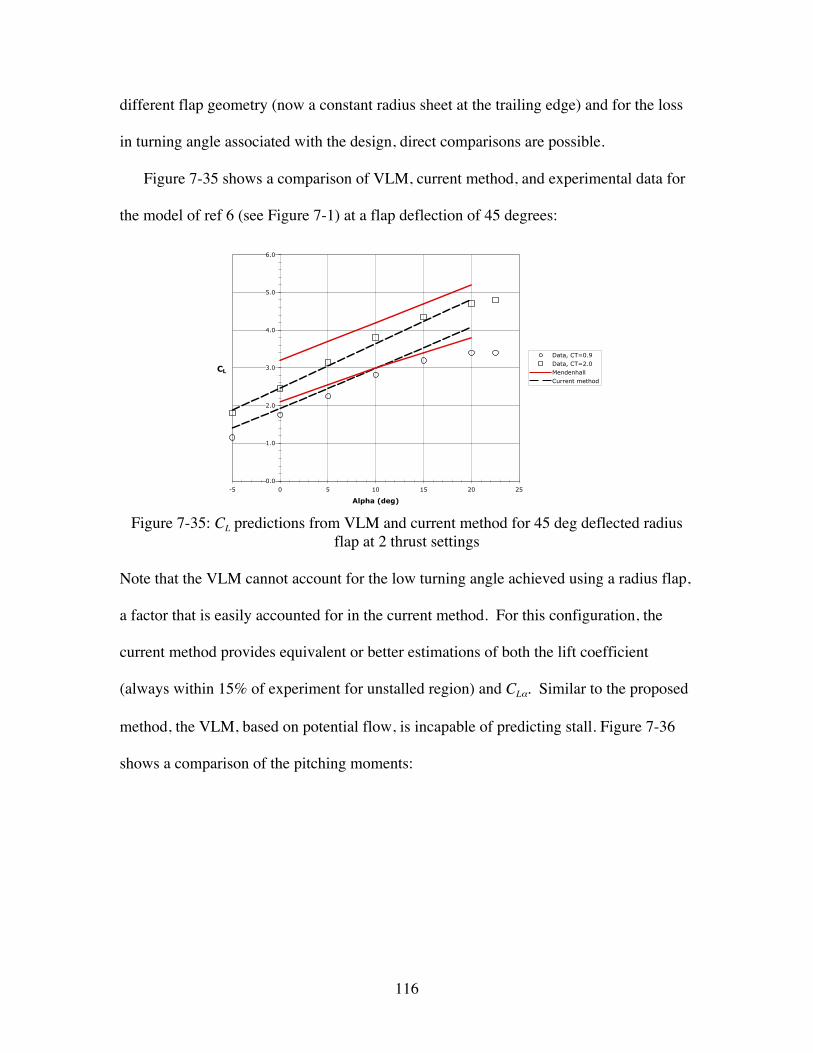
116
different flap geometry (now a constant radius sheet at the trailing edge) and for the loss
in turning angle associated with the design, direct comparisons are possible.
Figure 7-35 shows a comparison of VLM, current method, and experimental data for
the model of ref 6 (see Figure 7-1) at a flap deflection of 45 degrees:
0.0
1.0
2.0
3.0
4.0
5.0
6.0
-5 0 5 10 15 20 25
Alpha (deg)
CL
Data, CT=0.9Data, CT=2.0MendenhallCurrent method
Figure 7-35: CL predictions from VLM and current method for 45 deg deflected radiusflap at 2 thrust settings
Note that the VLM cannot account for the low turning angle achieved using a radius flap,
a factor that is easily accounted for in the current method. For this configuration, the
current method provides equivalent or better estimations of both the lift coefficient
(always within 15% of experiment for unstalled region) and CLα. Similar to the proposed
method, the VLM, based on potential flow, is incapable of predicting stall. Figure 7-36
shows a comparison of the pitching moments:
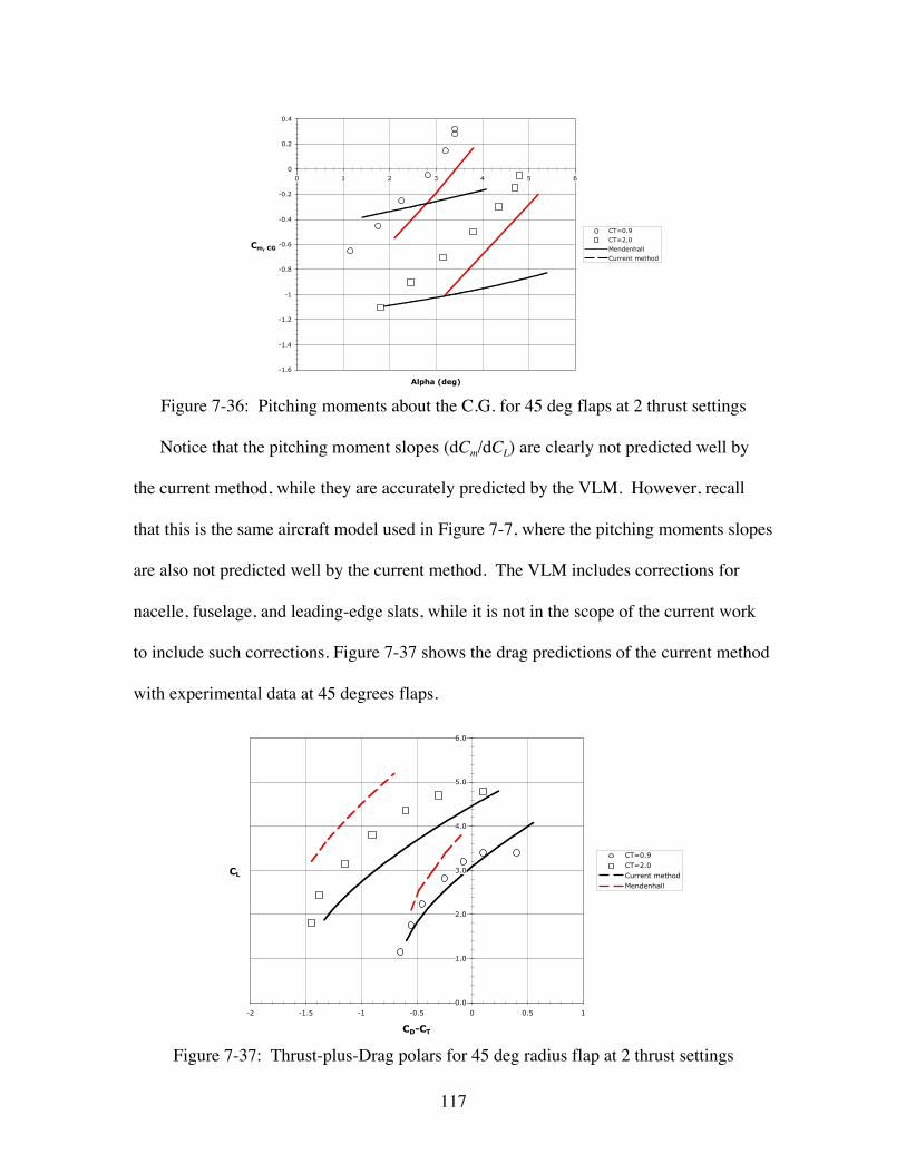
117
-1.6
-1.4
-1.2
-1
-0.8
-0.6
-0.4
-0.2
0
0.2
0.4
0 1 2 3 4 5 6
Alpha (deg)
Cm, CG
CT=0.9CT=2.0MendenhallCurrent method
Figure 7-36: Pitching moments about the C.G. for 45 deg flaps at 2 thrust settings
Notice that the pitching moment slopes (dCm/dCL) are clearly not predicted well by
the current method, while they are accurately predicted by the VLM. However, recall
that this is the same aircraft model used in Figure 7-7, where the pitching moments slopes
are also not predicted well by the current method. The VLM includes corrections for
nacelle, fuselage, and leading-edge slats, while it is not in the scope of the current work
to include such corrections. Figure 7-37 shows the drag predictions of the current method
with experimental data at 45 degrees flaps.
0.0
1.0
2.0
3.0
4.0
5.0
6.0
-2 -1.5 -1 -0.5 0 0.5 1
CD-CT
CL
CT=0.9CT=2.0Current methodMendenhall
Figure 7-37: Thrust-plus-Drag polars for 45 deg radius flap at 2 thrust settings
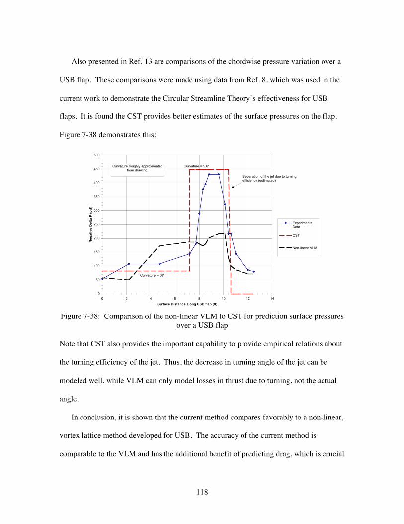
118
Also presented in Ref. 13 are comparisons of the chordwise pressure variation over a
USB flap. These comparisons were made using data from Ref. 8, which was used in the
current work to demonstrate the Circular Streamline Theory’s effectiveness for USB
flaps. It is found the CST provides better estimates of the surface pressures on the flap.
Figure 7-38 demonstrates this:
0
50
100
150
200
250
300
350
400
450
500
0 2 4 6 8 10 12 14
Surface Distance along USB flap (ft)
Neg
ativ
e D
elta
P (
psf
)
ExperimentalData
CST
Non-linear VLM
Separation of the jet due to turning efficiency (estimated)
Curvature roughly approximated from drawing.
Curvature = 33'
Curvature = 5.6'
Figure 7-38: Comparison of the non-linear VLM to CST for prediction surface pressuresover a USB flap
Note that CST also provides the important capability to provide empirical relations about
the turning efficiency of the jet. Thus, the decrease in turning angle of the jet can be
modeled well, while VLM can only model losses in thrust due to turning, not the actual
angle.
In conclusion, it is shown that the current method compares favorably to a non-linear,
vortex lattice method developed for USB. The accuracy of the current method is
comparable to the VLM and has the additional benefit of predicting drag, which is crucial

119
for USB designs. The weaknesses of the current method are typically shared with the
VLM, such as the inability to predict stall and the need for empirical information about
the jet. Without an iterative solution for the jet boundaries, the time required to run each
method is likely comparable. While the current method would require the generation of
new 2-D data for variations in thrust or flap setting, the VLM would require the
recalculation of the influence coefficient matrix. Given the prospect for growth of the
current method, we believe it is a more appropriate, robust tool for the conceptual design
stages of USB aircraft.

120
Chapter 8: Conclusions and Recommendations
The current work has introduced a methodology for the aerodynamic performance
predictions of USB aircraft for use in the conceptual and preliminary design phases. We
have described the new approach, correlated it with available 2-D data, and presented
comparisons of predictions with published USB data. The current approach has been
shown to produce good results over a broad range of propulsion system parameters, wing
geometries, and flap deflections. In addition, the semi-analytical nature of the
methodology will lend itself well to aircraft design programs/optimizers such as
ACSYNT. These factors make the current method a useful tool for the design of USB and
USB/distributed propulsion aircraft.
It is important to understand the limitations of the proposed methodology. These
limitations stem from two main sources: 1). limited empirical relations developed using
available 2-D data, and 2). numerical limitations within the modified Weissinger method
implementation (high-lift module). The first source was anticipated, and is due to the
limited amount of 2-D USB data available that is suitable for creating empirical relations.
121
It is believed that the current predictions could be significantly enhanced by a dedicated
experimental study of 2-D USB sections with trailing edge devices. Due to lack of 2-D
data involving flaps, confidence in the predictions of the current method decrease with
increasing flap angle. In addition, the method begins to break down for large blowing
coefficients (see the correlations in Chapter 5).
The second limiting factor of the current method is the High-Lift module calculations.
Chapter 6 offers a more detailed look at these problems. Breakdown and modification of
this code is beyond the scope of the current work, and thus known problems were
corrected by post-processing of the output. The usability of the current method would be
greatly enhanced by additional work on the High-Lift module specifically directed
towards modeling wings with powered-lift wings. Some ideas in this area have already
been offered by Chattot(58), and focus primarily on improving the convergence of the
solution in cases where the effective angle of attack becomes large.
The current work has been shown to be a useful tool for predicting longitudinal
aerodynamic characteristics of low-speed USB wings at low-to-moderate angles of
attack. However, the possibilities for future work are abundant. In addition to wind-
tunnel work on 2-D USB characteristics, providing the capability to predict the stall/CLmax
of a USB wing would be very useful. Also, since engine-out performance is usually an
active constraint on design, estimations of the lateral-directional characteristics are
important. This capability would require only minor modifications to the High-Lift
module. Future studies in these directions could significantly enhance the current
method’s relevance to USB aircraft design.

122
References
1. http://www.cnn.com/2004/TRAVEL/07/28/ohare.delays.html
2. http://www.flightdailynews.com/farnborough2004/07_19/airtransport/mega.shtm
3. http://sats.larc.nasa.gov/main.html
4. Hange, Craig, “Trajectory Kinematics of a Simultaneous Non-InterferingLanding Approach, and the Impact on ESTOL Regional Transport Performanceand Flight Control”, AIAA Paper 2003-6857, Nov., 2003.
5. Wimpress, John K., Newberry, Conrad F., The YC-14 STOL Prototype: ItsDesign, Development and Flight Test, AIAA Case Study, AIAA, Reston, 1998.
6. Sleeman, William C. Jr., Hohlweg, William C., “Low-Speed Wind TunnelInvestigation of a Four Engine Upper Surface Blown Model having a Swept Wingand Rectangular and D-Shaped Exhaust Nozzles”, NASA TN D-8061, Dec. 1975.
7. Riddle, D.W., et al, “Powered-Lift takeoff performance characteristics determinedfrom flight test of the Quiet Short-Haul Research aircraft”, AIAA 81-2409, AIAAFlight Testing Conference, Las Vegas, NV, Nov. 1981.
8. Sussman, M.B., Reed, J.B., O’Keefe, J.V., and Eldridge, W.M., “USBEnvironment Assessment Based on YC-14 Flight Test Measurements”, AIAAPaper 77-0593, 1977.
9. http://www.globalsecurity.org/military/systems/aircraft/amst-pics.htm.
10. http://ails.arc.nasa.gov/Images/Aeronautics/AC80-0613-3.html
11. Davis, Paul, “Industrial Strength Optimization at Boeing”, SIAM News, Vol. 29,No. 1, Jan/Feb, 1996.
12. Roberts, D.W., “A Zonal Method for Modeling Powered-Lift Aircraft FlowFields”, NASA CR-177521, March, 1989.
13. Mendenhall, M.R., Spangler, S.B., “Calculation of the longitudinal aerodynamiccharacteristics of upper-surface-blown wing-flap configurations”, NASACR-3004, 1978.
14. Spence, D.A., “The Lift Coefficient of a Thin, Jet-Flapped Wing”, Proceedingsof the Royal Soc., Series A, Vol. 238, pp. 46-68, Dec., 1956.
15. Mason, William, “Applied Computational Aerodynamics”, 1997

123
16. Smith, A.M.O., “High-Lift Aerodynamics”, Journal of Aircraft, Vol. 12, No. 6,pp. 501-530, 1975.
17. Korbacher, G.K., “Aerodynamics of Powered High-Lift Systems”, Annual Reviewof Fluid Mechanics, 1974.
18. Lan, C.E., Campbell, J.F., “A Wing-Jet Interaction Theory for USBconfigurations”, Journal of Aircraft, Vol. 13, No. 9, 1976, pp. 718-726.
19. Shollenberger, C.A., “Analysis of the Interaction of Jets and Airfoils in TwoDimensions”, Journal of Aircraft, Vol. 10, No. 5, 1973, pp. 267-273.
20. Karamcheti, K., Principles of Ideal-Fluid Aerodynamics, Wiley and Sons, 1966.21. Siestrunck, R., “General Theory of the Jet Flap in Two-Dimensional Flow”,
Boundary Layer and Flow Control, Ed. G.V. Lachmann, Vol. 1, Pergamon Press,New York, 1961, pp. 342-362.
22. Englar, Robert J., “Circulation Control Pneumatic Aerodynamics: Blown Forceand Moment Augmentation and Modification; Past, Present & Future”, AIAAPaper 2000-2541, 2000.
23. Helmbold, H.B., “Theory of the Finite-Span Blowing Wing”, Journal of theAeronautical Sciences, Vol. 23, May 1957, pp. 339-370.
24. Davenport, F.J., and Hunt, D.N., “Deflection of a Thick Jet by a Convex Surface:A Practical Problem for Powered Lift”, AIAA Paper 75-0167, 1975.
25. Schetz, J.A., Boundary Layer Analysis, Prentice Hall, Englewood Cliffs, NJ, 199326. Launder,B.E., and Rodi, W., “The Turbulent Wall Jet”, Progress in Aerospace
Science, Vol. 19, No. 2, 1983.
27. McCormick, Barnes W., Aerodynamics of V/STOL Flight, Dover Publications,New York, 1999.
28. Phelps, Arthur E., et al, “Summary of Low-Speed Aerodynamic Characteristics ofUpper Surface Blown Jet-Flap Configurations”, Powered Lift Aerodynamics andAcoustics, pp. 63-87, 1976.
29. Henderson, Campbell, and Walters, Marvin, “High-Lift STOL Aerodynamics /Stability and Control Techniques Assessment”, Naval Air Development CenterReport No. 81261-60, March, 1983.
30. Ryle, D.M. Jr., Braden, J.A., and Gibson, J.S., “Upper Surface BlowingAerodynamic and Acoustic Characteristics”, AIAA Paper 77-0608, 1977.
124
31. Narain, J.P., “Viscous-Inviscid Simulation of Upper Surface BlownConfigurations”, AIAA Paper 84-2200, 1984.
32. Rooney, Eugene C., “Thrust-Drag Accounting Methodology”, Thrust and Drag:It’s Prediction and Verification, ed. Covert, Eugene E., Progress in Astronauticsand Aeronautics, Vol. 98. AIAA, New York, pp. 29-45, 1985.
33. Bowers, Douglas and Tamplin, Gordon, “Throttle-Dependent Forces”, Thrust andDrag: It’s Prediction and Verification, Ed. Covert, Eugene E., Progress inAstronautics and Aeronautics, Vol. 98. AIAA, New York, pp. 207-279, 1985.
34. Wimpress, John K., “Upper Surface Blowing Technology as applied to the YC-14Airplane”, SAE paper 730916, 1973.
35. May, Fred W., and Bean, George E., “Aerodynamic Design of the Boeing YC-14Advanced Medium STOL Transport”, AIAA Paper 75-1015, 1975.
36. Hough, G.R., “A Study of the Blown Flap/Jet Flap Analogy”, AIAA Paper79-0119, 1979.
37. Gainer, Thomas G., Yip, Long P., Vogler, Raymond D., “Comparison ofAerodynamic Theory and Experiment for Jet-Flap Wings” Powered-LiftAerodynamics and Acoustics, NASA SP-405, pp. 103-118, 1976.
38. Spence, D.A., “The Lift on a Thin Aerofoil with a Jet-Augmented Flap”, TheAeronautical Quarterly, August 1958, pp 287-299.
39. Davis, W.H. Jr., “Extension of Spence’s Jet-Flap Theory for Thin Airfoils toAccount for Camber Effects”, Grumman Memo EG-ARDYN-79-08, 1979.
40. Roberts, L., “A Theory for Turbulent Curved Wall Jets”, AIAA Paper 87-0004,1987.
41. Torenbeek, Egbert, Synthesis of Subsonic Airplane Design, Delft UniversityPress, 1981.
42. Roberts, C.R., “An Experimental Investigation of a Powered Wing in Two-Dimensions”, M.S. Thesis, University of Texas at Arlington, 1984.
43. Pernice, Ciro, “An Experimental Study of a Two-Dimensional Propulsive Wing”,M.S. Thesis, University of Texas at Arlington, 1986.
44. Jeon, C.S., “Experimental Study of a Two-Dimensional Propulsive Wing in aLow-Speed Wind Tunnel”, M.S. Thesis, University of Texas at Arlington, 1990.

125
45. Drela, M., “XFOIL: An Analysis and Design System for Low Reynolds NumberAirfoils”, Low Reynolds Number Aerodynamics, Lecture Notes in Engineering,Vol. 54, Springer-Verlage, June 1989.
46. Weissinger, J., “The Lift Distribution of Swept-Back Wings”, NACA TM 1120,1947.
47. Campbell, George S., “A Finite-Step Method for the Calculation of SpanLoadings of Unusual Planforms”, NACA RM L50L13, 1951.
48. Blackwell, James A., “A Finite-Step Method for Calculation of Theoretical LoadDistributions for Arbitrary Lifting-Surface Arrangements at Subsonic Speeds”,NASA TN D-5335, July, 1969.
49. Paris, John Kenneth Floyd, “Advancements in the Design Methodology forMulti-Element High-Lift Systems on Subsonic Civil Transport Aircraft”, M.S.Thesis, University of California at Davis, 1996.
50. Vander Kam, Jeremy C., “Reduced-Order High-Fidelity Methodologies for theDesign of Civil Transport High-Lift Systems”, M.S. Thesis, University ofCalifornia at Davis, 2000.
51. Roberts, Michael M., “Improvement and Validation of a Reduced-Order High-Fidelity Methodology for Civil Transport Aircraft Design”, M.S. Thesis,University of California at Davis, 2003.
52. Raymer, Daniel P., Aircraft Design: A Conceptual Approach, AIAA EducationSeries, 1992.
53. Abbott, Ira H., Von Doenhoff, Albert E., Theory of Wing Sections, Including aSummary of Airfoil Data, Dover Publications, New York, 1959.
54. Smith, Charles C., Phelps, Arthur E., and Copeland, W., “Wind-TunnelInvestigation of a Large-Scale Semispan Model with an Unswept Wing and anUpper Surface Blown Jet Flap”, NASA TN D-7526, Feb., 1974.
55. Phelps, Arthur E., and Smith, Charles C., “Wind-Tunnel Investigation of anUpper Surface Blown Jet-Flap Powered-Lift Configuration”, NASA TN D-7399,Dec., 1973.
56. Recktenwald, Gerald, Numerical Methods with MATLAB, Prentice Hall, 2000.
57. Whitten, Perry D., “An Experimental Investigation of a Vectored-Engine-Over-Wing Powered-Lift Concept”, Technical Report AFFDL-TR-76-92, Dec., 1977.

126
58. Chattot, Jean-Jacques, “Analysis and Design of Wings and Wing/WingletCombinations at Low Speeds”, AIAA Paper 2004-220, Jan., 2004.

127
Appendix A: Annotated Bibliography
The purpose of this bibliography is to give the reader a sense of the previous work doneon this subject. The body of work that follows was the main base of information for thedevelopment presented in this thesis. It will also hopefully serve as a reference tool foranyone seeking a particular topic concerning USB. The sources have been broken intomain categories based on the nature of the work done. Within these groups, sources arelisted alphabetically by author and then chronologically. The main categories are:
- Powered-Lift Theory- Experimental Research- Flight Test Research- Inviscid/Panel Method Developments- Computational Fluid Dynamics Developments- Analytical Developments
This list is certainly not a complete list of work on the subject of Upper Surface Blowing,nor is it limited to sources cited in the report.
A-1: Powered-Lift Theory
♦ Henderson, Campbell, and Walters, Marvin, “High-Lift STOL Aerodynamics /Stability and Control Prediction Techniques Assessment”, Naval Air Systems CommandReport No. 81261-60, pp 45-62, March, 1983.
This is an excellent reference that offers a good description of USB in addition toIBF, EBF, CCW, and vectored thrust. It combines the research of many sources into acomprehensive look at USB. The basic aerodynamics are described as being similar toIBF, with good correlation coming from the momentum flux coefficient and deflectionangle. A significant performance difference results from changes in flow turningefficiency. This idea is defined, and the primary variables that effect it are discussed.Plots of turning angle and turning efficiency are presented against several geometricparameters.
The high-lift performance of USB configurations is then discussed and plotspresented of typical lift and pitching moments. The lateral-directional characteristics arealso discussed briefly. A potential flow solution method created by Mendenhall andSpangler (this work is summarized later in this appendix) is presented and therequirements/assumptions discussed. The method is a non-linear vortex lattice methodthat uses separate systems for the wing and engine wake to help capture the wing-wakeinterference effects. Similar limitations are faced in this method as in the current method.Complications are still present involving the unknown boundary and shape of the jet.Empirical relations must still be introduced to iteratively solve for these parameters. Acomparison with experimental results is presented and shows that the agreement is

128
generally similar to that produced in this thesis, though the lift performance is typicallyover-predicted.
♦ Helmbold, H.B., “Theory of the Finite-Span Blowing Wing”, Journal of theAeronautical Sciences, Vol. 23, May 1957, pp 339-370.
This paper focuses primarily on a three-dimensional wing with blowing, but alsoprovides a very good discussion on the features of two-dimensional flow. Although jet-flap theory was still in its early days when this paper was written, a qualitative knowledgeof the flowfield was developing. The physical principle behind blowing is that lift isgained by the jet reaction force, and further lift is gained by “jet-induced” lift. Thisinduced lift is a consequence of the jet sheet modifying the pressure distribution on theairfoil.
For a two-dimensional blown airfoil, a thin jet is blown down at some angle, δ.The pressure discontinuity across the sheet serves to turn the sheet back parallel with thefreestream direction. This is the source of our thrust recovery. The resultant of thispressure distribution over the jet can be viewed as a “turning force” which has a lift anddrag component. The lift is our reaction lift. By the Kutta-Joukowski theorem, the nethorizontal force must be zero, so our drag component is exactly balanced by the leading-edge suction force or leading-edge thrust. Since we’ve assumed inviscid flow, the lift istaken to be the sum of the reaction force, basic airfoil lift (without blowing), and theinduced circulation lift.
The three-dimensional discussion highlights the effect a finite span has onblowing. The primary new effect is the presence of induced drag, which can besignificant is these cases. In addition, there are losses of jet thrust and jet-induced lift.The loss of lift is a result of a decrease in curvature of the jet sheet.
♦ Korbacher, G.K., “Aerodynamics of Powered High-Lift Systems”, Annual Review ofFluid Mechanics, 1974.
This paper presents a link between mechanical high-lift systems and poweredhigh-lift systems. It offers useful analogies and a very thorough treatment of powered-liftaircraft. It begins with a broad look at the need for and the factors behind powered-liftdesigns for STOL or V/STOL aircraft. This includes field length considerations as wellas range, noise, and cost factors. The different methods of using power to augment liftare then discussed, beginning naturally with boundary layer control. A good discussionof the jet-flap is presented. The change from BLC to powered-lift is also discussed. Theremainder of the paper deals with other powered-lift concepts in turn.
129
♦ Smith, A.M.O., “High-Lift Aerodynamics”, Journal of Aircraft, Vol. 12, No. 6, pp501-530, 1975.
This well-known paper is one of the most fundamental pieces of literatureavailable on mechanical high-lift devices. Although the methodology used in portions ofthe paper is now outdated, much of the work centers on the theory for high-liftperformance. The need for high-lift is presented along with a survey of high-lift devicesand their capabilities. The majority of the paper deals with the ability of boundary layersto endure the pressure gradients that mechanical high-lift devices impose. An excellentdiscussion of multi-element flap systems is included, and shows the reasons why suchfavorable interference can occur between flap elements.
Only a small portion of the paper is devoted to power-augmented lift. Hisdiscussion is geared more towards the use of power to control the boundary layer, butthese concepts have a broader application. It is determined that the use of suction todelay separation is only effective when small delays are needed. The use of tangentialblowing is preferred. He describes tangential blowing as “making up for the momentumlost in the boundary layer”. Tangential blowing leads to discussions of early circulationcontrol airfoils. He notes that a “drag bucket” exists for blown airfoils operating at lowblowing coefficient values where the problems of separation are alleviated and haveresidual thrust from the blowing. Smith also makes an excellent point, as shown by manyother researchers, that if a trailing jet is deflected, it will carry a load. Thus it is possibleto carry load all the way to the trailing edge of the airfoil and the pressure recoveryproblem is eliminated.
A-2: Experimental Research
♦ F.J. Davenport, D.N. Hunt, “Deflection of a Thick Jet by a Convex Surface: APractical Problem for Powered Lift” AIAA Paper 75-167, January 20, 1975.
This paper describes work performed by the Boeing Company using a simplifiedUSB configuration to examine factors driving performance. Since the jet turningefficiency of a thick wall jet is of primary importance, this effect was the focus of thestudy. Simultaneous experimental and analytical programs were conducted. Only 2-Dflow was studied for simplicity, and based on the assumption that the planar-flow caseprobably represents an upper limit to jet turning performance.
A good statement of the fundamental problems faced by USB was included. Itwas found that the most powerful parameter governing jet turning by a convex surface(Coanda effect) is the ratio of jet depth to the radius of curvature. Three processes wereidentified that affect USB flow: 1. Mixing layers that reduce flow curvature and thusturning efficiency, 2. BL separation in the adverse pressure gradient between the flapknee and TE, and 3. local acceleration in the jet to supersonic speeds incurringmomentum losses.
The experimental program used a small scale model capable of variations in TEradius of curvature and flap angle. (The “flap” consisted of a circular arc) The model
130
also allowed for variations in jet thickness. Experiments conclude that the larger the ratioof radius of curvature to jet thickness, the greater the attainable jet deflection becomes.Measurements done of pressure coefficients on the surface show that compressibilityeffects also become important with increasing freestream dynamic pressure (this impliesthat USB flows are still quite sensitive to freestream dynamic pressure even though thejet dynamic pressure may be very much higher). Separation of the jet from the flapsurface, in essence a decrease of the jet turning efficiency, was seen to occur earlier withincreasing freestream dynamic pressure
The analytical model developed was to calculate the 2-D performance and flapsurface pressures assuming incompressible, inviscid conditions. The solid wingboundary was represented as a bound vortex sheet, the boundaries of the jet were freevortex sheets, while the jet flow was modeled by a source partially enclosed by the foldedback airfoil leading edge. The boundary conditions were no flow across any vortex sheet,and no pressure discontinuity across the free vortex sheets. These sheets were broken upinto small line elements of linearly-varying vorticity, and a typical matrix system wassolved for the sheet strengths.
The results of the potential flow model demonstrated good agreement for thewind-off condition. An important result was noted that potential flow, as opposed tomixing or other viscous effects, is accountable for much of the jet turning angledeficiencies. The wind-on conditions also agreed reasonably well for low jet Machnumbers. Naturally, as Mjet increases, the potential flow model does not predict the flowwell. It was concluded that USB flows must be understood with the presence of externalfreestream flows, and that the effects of compressibility should be included. Proper USBflap contouring is necessary to ensure good wind-on jet turning.
♦ Englar, Robert, J., “Investigation into and Application of the High VelocityCirculation Control Wall Jet for High Lift and Drag Generation on STOL Aircraft”,AIAA Paper 74-0502, 1974.
The paper examined the basics of trailing edge circulation control to augmentairfoil performance. Although it is primarily for a blunt trailing edge with tangentialblowing, many of the principles apply to jet-flaps and consequently USB. It was clearlydemonstrated that circulation control greatly increases lift and comes with associatedincreases in drag. The scale of momentum coefficients examined is approximately anorder of magnitude lower than typical jet-flap coefficients. This is because without asharp trailing edge, circulation control is easier to achieve (moving the rear stagnationpoint is easier). Also, the lift increase comes almost exclusively from circulation lift,since the jet reaction is very small.
The creation of additional profile drag is briefly addressed. As blowing increases,the profile drag is shown to increase. Englar describes this as the result of the jet actuallybeing turned into the lower surface flow, and could also be from the “leading edge” typeof flow behavior now present at the trailing edge. Several 2-D investigations were donewith an airfoil that could go from a conventional sharp TE at cruise to a full, blunt TEcirculation control airfoil using a clever flap design. The intermediate stages basically
131
functioned as an internally blown flap. Much study was done on jet detachment, sincethis will greatly affect the location of the rear stagnation point.
Pressure coefficients around the airfoil were presented, demonstrating the classic“saddle-back” shape with low LE expansion pressures and even lower coanda surfacepressures at the TE. Shear stress over the TE demonstrates that the jet very quicklytransitions to a turbulent inner region. Results from 3-D testing were also included. Fora flap deflection of 180 deg, the drag increases in a regular fashion with increasingblowing coefficient. At this condition, there is no thrust recovery due to the larger wakementioned above. At a deflection of 45 deg, where the airfoil is functioning more like aninternally blown flap, the drag is shown to decrease as blowing increases. This isbecause the jet efflux momentum begins to be recovered as thrust. Based on theircalculations, up to 70% of the jet momentum was recovered as thrust. The balance of thismomentum can be viewed as lost in jet turning or additional drag penalties withincreasing blowing. (Theoretically we recover all the thrust)
♦ Gainer, Thomas G., Yip, Long P., Vogler, Raymond D., “Comparison ofAerodynamic Theory and Experiment for Jet-Flap Wings”, NASA SP-405, 1978.
Comparisons were made with extensive experiments performed at the LangleyV/STOL wind tunnel. Two types of jet-flaps were tested: a pure jet-flap and jet-flapblowing from the knee of a small trailing edge flap (essentially internally blown flaps).Full and partial-span blowing was investigated for wing aspect ratios of 8.0 and 5.5 overa range of momentum coefficients from 0 to 4. Forces and moments were measuredusing a strain-gage balance, and pressure data was recorded at 6 spanwise locationsacross the semispan. For the blown flap, measurements were made at 0, 15, 30, 45, and60 degrees. Theoretical predictions were made using a Elementary Vortex Distributionprogram developed at McDonnell-Douglas, which is a basically an implementation ofSpence’s jet-flap theory. Some time was spent describing the program, but betterprograms are currently in use.
For the pure jet-flap, the lift, drag, and pitching moment were found to be inexcellent agreement with theoretical predictions regardless of the span of blowing. Thelone exception was for a blowing coefficient of zero, where the flow had a good deal ofseparation. The drag values were shown to be very high, but due primarily to induceddrag. Since good agreement was seen with the theory, which assumed 100% leadingedge suction, the model experienced full thrust recovery. The pressure distributions werealso presented, and it was seen that the theory underpredicted the pressure coefficients.Thus, the total lift was in good agreement although the components (circulation lift,reaction lift) were different.
For the blown jet-flap, the theory consistently underpredicted the lift, drag, andpitching moment. These results lead to the (now proven correct) conclusion that there isa substantial interaction between the jet exhaust passing over the deflected flap that wasnot being accounted for by the theory. This effect is clearly seen in looking at thepressure coefficient distributions at a spanwise station with blowing. There is asignificant suction area over the flap and it extends forward of the flap knee.
132
♦ Hough, G.R., “A Study of the Blown Flap/Jet Flap Analogy”, AIAA Paper 79-0119,1979.
A study was done to examine the validity of using jet flap analysis on moreadvanced propulsive lift systems. The systems studied were the jet-augmented flap(IBF), externally blown flaps (EBF), and upper surface blowing (USB). Analyticalpredictions were made using a modified lifting line and optimized vortex lattice methods.The “jet flap analogy” suggests that a blown flap system will behave aerodynamicallylike a jet flap system having the same spanwise distribution of jet momentum.Experimental data was obtained from separate sources for each of the three lift systemsmentioned above.
To carry out the comparison for a particular design, we need to know the trailingedge jet strength, its spanwise distribution, and jet deflection angle in addition to thebasic wing geometry. While it is understood that simple jet flap theory cannot accuratelypredict the complete forces and moments, this study was done to demonstrate that jet flaptheory can predict incremental changes in forces and moments due to changes in inputparameters. Classic jet flap theory is unable to reflect the true magnitude of the forcesand moments because wing and jet thickness effects aren’t modeled, nor are the viscousinteractions of the wing/jet. The nomenclature used in this paper is very similar to thatused in this thesis where CT is the total jet momentum coefficient (basically the grossthrust coefficient), and Cµ is the local momentum coefficient (local 2-D coefficient).
It was found that jet flap theory does indeed approximate the changes in forcesand moments well. While the magnitude of these quantities were consistently under-predicted, incremental changes due to changes in wing geometry, angle of attack,blowing coefficient, and engine configuration were predicted fairly well. The predictionswere shown to be within 10% of the expected values for any given configuration.
♦ Pernice, Ciro., “An Experimental Study of a Two-Dimensional Propulsive Wing”,M.S. Thesis, University of Texas at Arlington, 1986.
This experimental work was done in the low-speed wind tunnel at U.T.A. Asmall model was built that had a two-dimensional nozzle located at the 70% chordlocation on the upper surface. The wing section was based on an NACA 0025 airfoil.Propulsive flows were simulated using compressed air. The primary data taken werepressure measurements around the surface at the mid-span location where the flow wasverified to be two-dimensional. Force and moment calculations were attained byintegration of these pressures. All coefficients were based upon the chord and a unitspan, and thus are sectional coefficients.
Tests were performed at angles of attack of –5, 0, 5, 10, and 15 degrees over arange of dynamic pressures (1.0, 5.0, and 10.0 lb/ft2) and jet momentum coefficients (0.0– 3.0). Wake surveys were also obtained, but only used for qualitative analysis. Plots ofCl, Cm(c/4), and Cd versus momentum coefficient are presented. Variations with angle ofattack are also shown. A good discussion on the use of Cj (jet momentum coefficient) ispresented and it is determined that this factor is not suitable for low blowing cases or for
133
cases where the external flow approaches the jet velocity. A more suitable parameter forcorrelation is the “net momentum coefficient” (Cfn). However, within the range of typicaldesigns, both parameters work well.
The direct entrainment of external fluid by the jet was also studied. It was shownthe fluid upstream of the nozzle exit reached higher velocities as the blowing coefficientincreased. Minimal discussion on the drag and pitching moment are included, though thepressure drag, Cdp, was deemed “unreasonably large”. A key to this document’susefulness is the inclusion of the data sheets for each point presented. This allowsaccurate models to be built of the compressed air propulsion system and serves as anexcellent check to analysis.
♦ Phelps III, A.E., Johnson, J.L, and Margason, R.J., “Summary of Low-SpeedAerodynamic Characteristics of Upper-Surface-Blown Jet-Flap Configurations”,Powered Lift Aerodynamics and Acoustics, pp. 63-87, 1976.
This paper provided a very good overview of the important characteristics thatdetermine USB performance, stability, and trim. The former is all that is reported here.Of primary importance was the notion that low-speed performance is mainly dependentof the jet turning angle and turning efficiency. This in turn requires the use of properleading and trailing edge treatment to prevent unwanted flow separation.
Also shown is that USB configurations exhibit a fairly “localized” flow behavior.This means that the effect of the jet flow does not spread much in a spanwise direction.This localized flow field may provide a means through which 2-D sectional data can beused to approximate the overall wing performance. A plot of the spanwise distribution ofnormal force for a USB configuration indicated that the influence of the exhaust jet onthe wing is contained is a region extending approximately 1.75 nozzle widths outboard ofthe nozzle.
The effects of Reynolds number on USB experimental data led to the conclusionthat the performance characteristics are dominated by the exhaust jet rather than thefreestream flow (recall that this is low speed flow however and compressibility effectsaren’t important). This improves the confidence with which small-scale data can be used.It was also observed that, in general, the nozzle geometries that produce good flowturning performance produce poor cruise performance characteristics.
The longitudinal and lateral-directional stability and trim were analyzed with theincreased performance of the wing. As expected, with increased lifting characteristics onthe wing, the tail volume required for trim increases dramatically. For lateral-directionalanalysis it was shown that wing swept introduced dynamic instabilities (dutch roll).Lastly, engine-out situations were considered. Naturally, this condition can be veryproblematic in USB configurations. Boundary Layer Control on the failed engine sidewas found to make conditions acceptable. (Note that BLC is a reasonable technology,especially since LE blowing could be used to eliminate premature LE separation due tosupercirculation)
134
♦ Roberts, Charles R., “An Experimental Investigation of a Powered Wing in TwoDimensions”, M.S. Thesis, University of Texas at Arlington, 1984.
This work was the predecessor to the above experimental work by Pernice. Assuch, the two are quite similar in the design of experiments. A model was created using aNACA 4412 airfoil with compressed air exhausting over the upper surface atapproximately 0.6 x/c. Force and moment data were taken over a range of angle of attackfrom –5 to 15 degrees, and dynamic pressures of 1.0, 5.0, and 10.0 lb/ft2. Based oncompressed air restrictions, blowing coefficients of only 0 - 2.8 were studied.
The data produced, however, does not seem wholly consistent with later work.The lift coefficients were indicated to be reaching a maximum value within the range ofblowing tested. The drag coefficients were also indicated to reach a maximum value. Itwas suggested by the author that these unexpected patterns were due to interferencebetween the jet and wind tunnel walls.
♦ Ryle, D.M., Braden Jr., J.A., and Gibson, J.S., “Upper Surface Blowing Aerodynamicand Acoustic Characteristics”, AIAA Paper 77-608, AIAA/NASA V/STOL Conference,June 1977.
This paper is basically a summary of exploratory work performed at Lockheedunder NASA Langley contracts. The aerodynamic work was largely experimental workon parametric changes in USB configurations. However, some theoretical correlationwas also performed. The following advantages over typical high-lift systems were givenfor USB configurations:
Very competitive High-Lift performanceAdaptive to Hybrid SystemsMechanical/Structural Simplicity, andCompetitive Acoustical Performance
The following disadvantages were also outlined:Inherently poor cruise configurationSensitivity of wing flow-field at cruise conditionConflicting high/low speed geometriesConflicting high lift/ acoustical performance
Extensive experimental data was taken for aerodynamic and acousticcharacteristics with changes in geometry. The theoretical modeling was used to supportthe experimental program and provide clarification of the flow phenomena. The basicpremise of the analytical work was to take an existing vortex lattice technique andsuperimpose nacelle and power effects on a given model. The jet emerging from thenacelle is modeled by an expanding, decreasing strength ring vortex system. Thus,“new” singularity panels can be added to account for power effects.
135
♦ Birckelbaw, L.D., “High Speed Aerodynamics of Upper Surface Blowing AircraftConfigurations” AIAA Paper 92-2611, AIAA Applied Aerodynamics Conference, June22, 1992.
This paper is focused nearly exclusively on experimental results of tests on a USBaircraft configuration. Particular emphasis is placed on the causes and magnitude of dragpenalties of twin and 4-engine USB configurations in high speed flow. These modelswere based on the Japanese “Aska” Quiet STOL aircraft. The effects of variations in thefree stream Mach number, angle of attack, engine power setting, and nacelle spanwiselocation are presented. Based on these effects, a generic set of design recommendationsare presented. No analytical methods were presented.
The results of the experiments found that high speed USB flows exhibit acomplex interaction of jet induced and wing transonic flow fields. The engine nacellescreated severe drag penalties that increased with freestream Mach number, power setting,and angle of attack. The presence of the nacelles and fuselage/nacelle effects alsoproduced strong upwash over the wing leading edge. (In addition to upwash producedfrom large jet turning angles) While it was found that a twin-engine configurationdeveloped more lift and less drag for engine speeds below 50,000 rpm, all configurationstested produced prohibitive drag increases at high speeds.
Based upon these findings, the author offers some design recommendations forgeneral USB configurations. First, the twin-engine design is preferable in terms ofperformance, but may not be preferable in terms of safety (engine out problems).Second, special filleting should be used at wing nacelle intersections to eliminate anyflow separation. Third, special consideration should be made to the wing L.E. in thepresence of increased upwash near the nacelles. Lastly, the engines should be as faroutboard and forward as possible to reduce interference effects with the fuselage. (Notethat this must be reconsidered for a twin-engine configuration)
A-3: Flight Test Research
♦ Sussman, M.B., Reed, J.B., O’Keefe, J.V., and Eldridge, W.M. “USB EnvironmentAssesment based on YC-14 Flight Test Measurements”, AIAA Paper 77-593, 1977.
This paper was a summary of flight tests and static rig tests of the environmentaround the USB flap of the Boeing YC-14. Static pressures, surface temperatures,surface fluctuations, and vibration levels were measured. This project was done byBoeing in conjunction with a NASA initiative. Wing and USB static pressure ports andthermocouples, along with high-frequency acoustic transducers were installed on thefuselage, engine nacelle, USB flaps, and upper suface behind the nozzle.
The results of testing for the upper surface/flap pressure measurements werepresented first. For a fixed USB flap setting, increasing thrust naturally generatesincreasingly negative pressures on the main flap section. The aft flap section changeswere smaller indicating a lesser contribution to turning effectiveness from this flap. For afixed power setting, increasing USB flap deflection induces larger suctions on the main
136
flap. The aft flap suctions increase until approximately 40 degrees where pressures thenbegin to decrease. Also, as expected, the turning efficiency is somewhat reduces in thepresence of a freestream. This is due to the stronger adverse pressure gradient thatdevelops on the aft side of the USB flap.
The temperature measurement were made in low-speed/takeoff and landingconditions where the USB system in full use. While the results may be very dependenton the particular configuration, the results were still reasonable. The main flapexperienced temperatures around 400 degrees F, with the aft flap around 250 deg. F. Thetemperatures measured on the body near the flap never exceeded 145 deg. F. Also, theflight temperatures were generally 50 to 100 degrees lower than these static rig results.Acoustic environment results were also presented but are not summarized here. It wasconcluded that the flight data and wind tunnel data agree fairly well, and that USB sonicand temperature data were less severe in flight conditions than predicted by static tests.
♦ Wimpress, J.K., and Newberry, C.F., “The YC-14 STOL Prototype: It’s Design,Development, and Flight Test”, AIAA Case Study, Reston, 1998.
The document is an extensive look at Boeing’s YC-14 STOL prototype, from theRFP to flight testing. Although it was originally written some time ago, it has beenupdated recently. Because the high-lift capabilities of the YC-14 were based around theconcept of USB, this document contains some interesting information on the backgroundof the idea and its implementation. Only material relating to this is summarized here.
The Boeing company first became interested in the USB concept in the late 60swhen the design implications of a jet’s tendency to adhere to an adjacent physical surfacewere first being realized. Their wind tunnel test program verified previous results andalso showed far greater thrust recovery than externally blown flaps. It was also seen thatL.E. BLC must be used to prevent premature separation and adequate control in anengine-out situation. Some of the test data taken was reported in this document and theyseem to agree with agree with conclusions reached in other papers – basically thateffective jet turning can be accomplished with appropriate design and that small scaleUSB testing models full scale USB configurations very well.
The nozzle design was a key feature in the success of the YC-14 design. Thenozzle outer contours were shaped to prevent high drag under cruise conditions. Inaddition, a small door was placed on the outboard side of the nozzle that would openduring high-lift operation. This door allowed the engine exhaust jet to spread furtheroutboard over the USB flap. It also increased the effective exit area. To increase jetturning performance, retractable vortex generators were placed near the T.E. of the basicwing. These generators came into use when flap deflections became large (>30°) andbasically increased mixing of the jet flow with the local boundary layer and delayed jetseparation until farther downstream.
An extensive boundary layer control system was also designed. Cross-ductingpermitted the continued use of BLC even in engine out cases. Interestingly, precautionshad to be made against any ruptures in this ducting, as it was shown that cabintemperatures would rise to fatal levels very quickly. The boundary layer control system,coupled with variable camber Krueger flaps, helped prevent premature flow separation
137
near the leading edge. Although this aircraft never reached production, it is still one ofthe only aircraft in existence to fully utilize upper surface blowing technology effectively.
A-4: Inviscid/Panel Method Developments
♦ Lan, C.E., and Campbell, J.F., “A Wing-Jet Interaction Theory for USBConfigurations”, Journal of Aircraft, Volume 13, No. 9, pp. 718-726.
This paper develops a linear, inviscid, subsonic compressible flow theory to treatthe interaction between a wing and an upper surface thick jet. Upper Surface Blowingproduces additional lift through this interaction, and through the jet entrainmentproducing the Coanda effect. Theoretically, an exact solution could be found fromanalysis of a three-dimensional turbulent wall jet in a wing flowfield. The methodpresented is for a wing in freestream Mach, Mo, with a thick jet of Mach number, Mj, onor above the wing surface. It is assumed that the flow fields (inside and outside of thejet) are governed by the Prandtl-Glauert equation.
The boundary conditions imposed were that the jet surface be a stream surfacewith static pressure continuous across it, and that the flow be tangential to the wingsurface. The wing is represented by a vortex distribution, while the jet surface ismodeled as 2 coincident vortex sheets (one to account for perturbations in the outer flow,one for the jet flow) Using quasi-VLM, additional vortex strengths induced on the wingcan be determined. Once the total vortex distribution on the wing is known, expressionswere determined for the aerodynamic forces and moments.
Some comparisons were made with experimental data (much more experimentaldata would be available at this point) and showed good results, particularly at smallflap/jet deflections. A comparison was made of predictions using thin jet flap theory, andit was shown that this theory is inadequate for predicting the aerodynamic characteristicsof USB configurations.
** A FORTRAN code was written for this method and is available in NASA report TM-X-73987
♦ Mendenhall, M.R., and Spangler, S.B., “Calculation of the Longitudinal AerodynamicCharacteristics of Upper-Surface-Blown Wing-Flap Configurations”, NASA CR-3004,1978.
This contractor report from NASA outlines the development of a non-linearvortex lattice method for the calculation of USB performance. Subsequently, the codeitself is printed in CR-3005. This methodology is the most useful and accurate of theinviscid methods investigated in the course of this work. It incorporates two potentialflow models for the wing and jet. The wing can have an arbitrary planform and the jet isassumed to be rectangular and have a fixed aspect ratio. It provides estimates of
138
chordwise pressure distributions, spanload distributions, total longitudinal coefficientsover a wide range of angles of attack and thrust settings.
The wing planform is unremarkable with the exception of the modeling of aconstant radius trailing edge flap. The semi-infinite legs of the trailing vortices areassumed to go to infinity in the plane of the last chordwise surface. The jet wake modelis comprised of vortex rings. The strength of the rings is determined through empiricalrelations concerning the jet spreading rates. The jet exit velocity is determined throughisentropic relations and the jet wake is assumed to maintain a constant aspect ratio. Thewake model provides an interference effect on the wing that mimics the physicalbehavior of USB.
Some corrections and extensions were created to provide estimations for thewhole aircraft. Fuselage and nacelle effects were modeled using slender body theory tocalculate lift forces and centers of pressure. Ram drag was also accounted for in thecode. Predictions were made using this methodology for several NASA experimentalUSB reports. These comparisons indicate that this method performs very well at lowangles of attack (unstalled regions) and at moderate thrust coefficients. The spanloaddistributions were predicted well, but the chordwise distributions were not. Drag wastypically under-estimated due to the lack of viscous effects in the calculations.
♦ Narian, J.P., “Viscous-Inviscid Simulation of Upper Surface Blown Configurations”,AIAA Paper 84-2200, AIAA Applied Aerodynamics Conference, Aug. 21, 1984.
This study investigates USB by using a combination of inviscid panel methodsand integral methods for viscous wall jets on curved surfaces in non-uniform flow. Thisstudy is a step in the direction suggested by Lan (see above). Study suggests thatviscous-inviscid methods involving panel methods and parabolized N-S solutions couldbe very effective, but were computationally expensive. This method uses a moreapproximate method where the inviscid flow field is solved by panel methods, then theentrainment velocity and plume boundaries of the jet are calculated using a 3-dimensionalintegral solution. Aft of the trailing edge, a “jet in cross-flow” theory is used.
The following process was used to obtain details on the jet behavior and pressuredistributions on the airfoil sections:
-The wing-body-nacelle configuration is analyzed via panel methods for theunpowered (flow-through) case-The pressure distribution at the nacelle centerline is used to calculate the non-uniform external velocities for the wall jet development-Integral analysis is used to determine the jet boundaries and jet entrainmentvelocities at several panel stations-The vorticity associated with the jet is imposed on the wall jet panels as a doubletgradient-The jet boundaries, prescribed entrainment velocities, and prescribed doubletgradient are used to create new panels to simulate the effects of jet blowing withinthe panel method.
139
Results on jet decay were then presented, and it was noted that convex curvature of thewall accelerates the decay of the wall jet, which results in rapid expansion of the jetboundaries. A USB model was tested experimentally and compared to theoretical resultswith favorable agreement. The lift coefficients predicted at various nozzle pressure ratiosagreed very well with experimental data. Pressure coefficient distributions were alsocalculated.
♦ Shollenberger, C.A., “Analysis of the Interaction of Jets and Airfoils in TwoDimensions”, Journal of Aircraft, Vol. 10, No. 5, pp. 267-273, 1973
A solution for the flow of a jet near one or more airfoils was developed. Flow isassumed to be inviscid, incompressible, and two-dimensional. The problem is governedby Laplace’s equation with a no-flow boundary condition enforced on the wing, as wellas across the jet. In addition, the jet involves a pressure boundary condition where thestatic pressure is constant across the jet boundary while velocity can be discontinuous.The velocity discontinuity is related to the total pressure difference between the jet andexternal streams. The primary difficultly involved defining a jet surface on which toapply these conditions.
The method of solution uses “flat-plate” airfoils modeled using vortex sheets.The jet boundaries can be modeled by vortex sheets whose strengths are related to thelocal mean velocity. The singularities of the airfoil are easy to determine since we set theairfoil position. The downstream jet is also easy to fix since its direction mustasymptotically approach the freestream direction. The near-field jet location can befound along with the singularity strengths in an iterative process. Some convergenceissues were discussed, including under-relaxation to improve convergence. Viscouseffects, which are of course ignored in an inviscid formulation, are described as confinedto the conventional boundary layer, and entrainment of the external fluid. Theentrainment could be empirically modeled by altering the boundary condition imposed onthe jet.
Some computations using this method were presented. The first is similar to anEBF system with a lower jet impinging on the lower airfoil surface and aft deflected flap.It was found that though a majority of the load was induced on the aft flap (smalldeflected flat plate), a significant load was induced on the main element even though itwas at zero angle of attack. The vertical position of a jet relative to an airfoil was alsoinvestigated. While a peak load was experienced when the airfoil was completelyimmersed, significant loadings were induced as the jet neared the upper or lowersurfaces.
140
A-5: Computational Fluid Dynamics Developments
♦ Bickelbaw, L., Atta, E., and Ragab, S., “Euler Solutions for Aircraft ConfigurationsEmploying Upper Surface Blowing”, Journal of Aircraft, Vol 24, No 3 pp 188-194
This paper outlines a zonal method for computing the flowfield around aircraftwith USB. This method is based on zonal grid generation coupled with an Euler flowsolver. A significant portion of this paper dealt with the grid generation and mating. Theflow solving technique was based on the Euler equations with a finite-volume time-stepping Runge-Kutta scheme. Artificial viscosity was added to the process through“dissipation constants”, and boundary conditions were typical for sub/supersonic cases.
Computations were initially run for 2-D cases (with 2 zones which represented theexhaust region and the rest of the flowfield). The process did capture the pressure peaksinduced by the jet and showed the expected variation with jet pressure ratio. The resultsfor 3-D were compared with experimental data and less complicated panel methods. TheEuler solutions performed very well with only some problems where nacelle effects weredominant and at the T.E. where viscous effects were dominant. This method may provevery effective but is not extremely useful in understanding what factors influence theflowfield changes.
♦ Roberts, D.W. “A Zonal Method for Modeling Powered-Lift Aircraft Flow Fields”,NASA-CR-177521, March 1989.
This paper is similar to the methods described by Narain (see above). Themethod described is a zonal method based on the coupling of a 3-D Navier Stokes code toa potential code. The coupling allows the appropriate modeling of the viscous/inviscidinteractions that dominate powered-lift configurations. Zonal methods involve dividingthe flow domain into a network of zones in which the simplest, appropriate flow analysisis used. Of key importance is the boundary conditions between the different zones.Since the potential flow is a subset of the N-S equations, the N-S zone must extend wellinto the region where viscous phenomena aren’t present. However, making the N-S zonetoo large can greatly increase computation time.
The panel method basically views the viscous zones as extensions of theconfiguration and are influenced through blockage effects and entrainment. Massconsveration is imposed going from N-S to panel zones. Similarly, the N-S method isinfluenced by the potential regions. The total pressure, temperature, and directioncosines of velocity are passed from the potential code to the N-S code. This paper goesinto some detail on the modifications made to the codes, and comparisons of results towind tunnel data. Although it appears that the correlation is very good, those results willnot be summarized here.
This method, while very powerful and accurate, may be too computationallyintensive for conceptual-level codes. The underlying principles of zonal methods may,however, be a very good way to approach USB configuration analysis.
141
A-6: Analytical Developments
♦ Davis, W.H. Jr., “Extension of Spence’s Jet-Flap Theory for Thin Airfoils to Accountfor Camber Effects”, Memo EG-ARDYN-79-08, Grumman Aircraft, 1979.
A parallel method was used to extend the analytical work of Spence (see below) to airfoilsections with parabolic camber. Similar-order curve fits were also presented. Since jet-flap theory is linear, this work “plugs-in” directly with the classical development. Aswith Spence, small disturbance theory was used to develop integro-differential equations.These were solved to form an additional term contributing the lift coefficient as:
€
ΔCl = 4π 1+ Co( )γ
where gamma is the maximum camber and Co is an empirically defined constantdependent on the blowing coefficient.
♦ Spence, D.A., “The Lift Coefficient of a Thin, Jet-Flapped Wing”, Proc. of the RoyalSociety of London, Series A, Vol. 238, Issue 1212, pp. 46-68, 1956.
This paper is widely recognized as one of the most important early works done onpowered lift. Spence recognized that lift is supplied not only by the reaction to thevertical momentum of the jet, but also by the modification of the surface pressures due tothe changes in the flowfield induced by the jet. The correlating parameter was taken tobe the momentum coefficient. It should be noted that the equation for this coefficient (eq34) does not explicitly show the chord length in the denominator since it is unity for thispaper. Since these are 2-D coefficients, it is also implied that these quantities are “perunit span”.
An analytical solution is given for the inviscid, incompressible flow past a thin,two-dimensional airfoil at reasonable angle of attack for which a thin jet emerges at thetrailing edge at some deflection angle, τ. The flow is also assumed irrotational, sopotential flow methods are used. The airfoil and jet are modeled using distributedsingularities and an “integro-differential” equation is obtained that is solved by cleverused of Fourier series. The basic equation is presented as:
€
Cl = 2πα + 4πBoα + 4πAoτ
where Ao and Bo are coefficients dependent on the momentum coefficient. A closeinterpolation to these coefficients is given for momentum coefficients between 0 and 10.
Similar data was given for the pitching moment, but was not developed into theconvenient form shown above. Pulling this data together was one purpose of this thesis.Some comparison with experimental data was performed and demonstrated the value ofthe theory. In the years since, the value of the theory (and the theory’s limitations) havebeen shown more completely.
142
Appendix B: Sample of Data Generation for 2-D Method
The purpose of this appendix is to provide an example of the typical process forgenerating/collecting the necessary input data for the 2-D methodology. The full 2-Dequations can be seen in equations (4-38) through (4-40) and clearly involve terms thatrequire a degree of knowledge about the configuration being studied. Further knowledgeabout the wing itself is needed to carry out 3-D performance calculations. For thepurposes of this appendix, the process of obtaining or calculating the necessary inputinformation for the Boeing YC-14 is presented.
B-1: Overview
In general, conceptual level analysis of Upper Surface Blown wing performancewill require information in 5 categories:
1. Planform Data – wing shape and size, engine locations, spanwiselocations of trailing/leading edge devices.
2. Flap Geometry – flap chord ratio, flap curvature and extension, flapdeflection angle, trailing edge angle of base airfoil
3. Approximate Nozzle Geometry – Nozzle height and width (or nozzleexit area), chordwise location of nozzle exit
4. Propulsion Data – aicraft total thrust coefficient, nozzle exit conditions5. Flight State Data – Mach number, altitude
This information is generally readily available for a conceptual design, or reasonableestimates can be made. Flap geometry and flap kinematics is the most detailed categoryby necessity, since this data will have a large effect on the performance. Once the data ofthe five categories has been calculated, estimated, or looked-up, the 2-D and 3-Dcalculation methods described in this work are straight forward to use and obtain goodresults.
B-2: Planform Data
Planform data is necessary primarily for the 3-D Weissinger calculations, butsome key pieces of information are also required for the 2-D approximations. In the caseof the YC-14, a significant amount of aircraft layout information was available. Technicaldrawings of the aircraft are available in the case study by Wimpress and Newberry(5). Inmost design cases, the planform information will not be as definite, and some quantitiesshould be judiciously approximated.
Figure B-1 shows a sketch of the YC-14 wing planform:
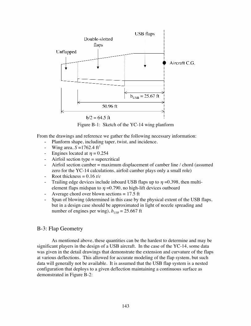
143
Figure B-1: Sketch of the YC-14 wing planform
From the drawings and reference we gather the following necessary information:- Planform shape, including taper, twist, and incidence.- Wing area, S =1762.4 ft2
- Engines located at η = 0.254- Airfoil section type = supercritical- Airfoil section camber = maximum displacement of camber line / chord (assumed
zero for the YC-14 calculations, airfoil camber plays only a small role)- Root thickness = 0.16 t/c- Trailing edge devices include inboard USB flaps up to η =0.398, then multi-
element flaps midspan to η =0.790, no high-lift devices outboard- Average chord over blown sections = 17.5 ft- Span of blowing (determined in this case by the physical extent of the USB flaps,
but in a design case should be approximated in light of nozzle spreading andnumber of engines per wing), bUSB = 25.667 ft
B-3: Flap Geometry
As mentioned above, these quantities can be the hardest to determine and may besignificant players in the design of a USB aircraft. In the case of the YC-14, some datawas given in the detail drawings that demonstrate the extension and curvature of the flapsat various deflections. This allowed for accurate modeling of the flap system, but suchdata will generally not be available. It is assumed that the USB flap system is a nestedconfiguration that deploys to a given deflection maintaining a continuous surface asdemonstrated in Figure B-2:
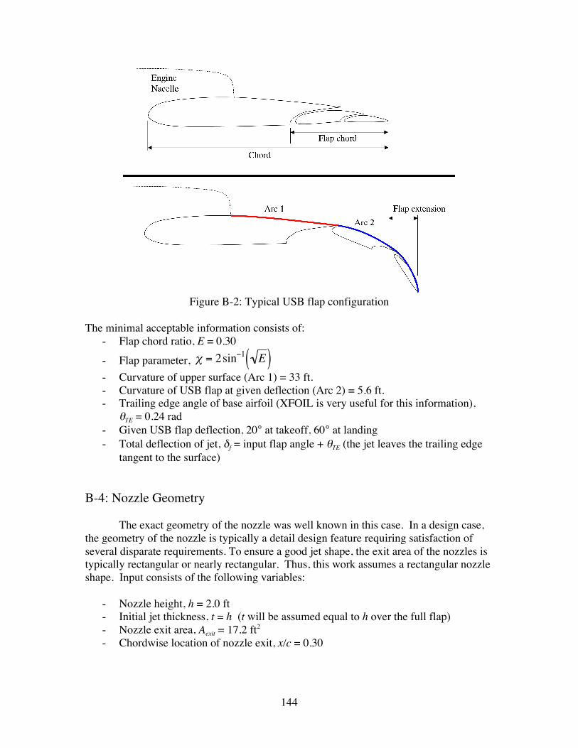
144
Figure B-2: Typical USB flap configuration
The minimal acceptable information consists of:- Flap chord ratio, E = 0.30- Flap parameter,
€
χ = 2sin−1 E( )- Curvature of upper surface (Arc 1) = 33 ft.- Curvature of USB flap at given deflection (Arc 2) = 5.6 ft.- Trailing edge angle of base airfoil (XFOIL is very useful for this information),
θTE = 0.24 rad- Given USB flap deflection, 20° at takeoff, 60° at landing- Total deflection of jet, δf = input flap angle + θTE (the jet leaves the trailing edge
tangent to the surface)
B-4: Nozzle Geometry
The exact geometry of the nozzle was well known in this case. In a design case,the geometry of the nozzle is typically a detail design feature requiring satisfaction ofseveral disparate requirements. To ensure a good jet shape, the exit area of the nozzles istypically rectangular or nearly rectangular. Thus, this work assumes a rectangular nozzleshape. Input consists of the following variables:
- Nozzle height, h = 2.0 ft- Initial jet thickness, t = h (t will be assumed equal to h over the full flap)- Nozzle exit area, Aexit = 17.2 ft2
- Chordwise location of nozzle exit, x/c = 0.30
145
B-5: Propulsion Data
For the case of the YC-14, it was known that CF6-50D engines were used.Appropriate data sheets contained the gross thrust, exit velocity, and mass flow rates forthese engines. Due to the use of Circular Streamline Theory, the exit conditions are vitalto the 2-D calculations. In a design case, where a rubber engine approach may be used,typically only the gross thrust may be specified. In this case, isentropic relations withsuffice to provide the exit conditions as follows. From the thrust:
€
TNet, Design Condition ≅ ˙ m Vexit −U∞( )
where the mass flow rate is:
€
˙ m = ρ jet AexitVexit
More exact relations involving nozzle pressure ratios are preferable to these basicrelations. The most critical propulsion parameter we must determine is the momentumflux coefficient or blowing coefficient for the 2-D calculations. This parameter assumesthat the engine operates at the design condition and is easy to find once the exitconditions are known:
€
Cµ = C j =˙ m Vexit
q∞cbUSB
where the dynamic pressure comes from flight-state data and c represents the averagechord over the blown section. For the YC-14, given total thrust coefficients of 1.0 and2.0, the relatively small blowing span produces 2-D blowing coefficients of 1.9 and 3.9,respectively.
B-6: Flight State Data
This data determines the freestream conditions the aircraft experiences. Thesemay vary significantly between points of interest, such as takeoff, landing, cruise, ormaneuver points.
- Altitude/Density, ρ∞ = 0.002377 sl/ft3
- Mach Number, M∞ = 0.1
146
Vita
Ernest Brock Keen was born on August 4, 1979 in Lebanon, Virginia. He grew up
there with his parents, Jack and Sheila, younger brother, Jordan, and older sister,Stephanie. After high school graduation, he moved to Blacksburg, Virginia to attend
Virginia Tech in Aerospace Engineering. As part of his undergraduate curriculum he was
a part of the Honors Program and the Co-operative Education Program. He spent onesemester with Allied Signal Aerospace Repair & Overhaul (now Honeywell) in Greer,
South Carolina. Another semester was spent working as a test engineer for Pratt &Whitney, Large Military Engines in Palm Beach Gardens, Florida. During his time at
Pratt & Whitney, he was a member of the Boeing test team for the CTOL qualification
engine for the X-32. He graduated Summa Cum Laude in May of 2002. Aftergraduating, he returned home for one year to assist in the development of his father’s land
surveying business. In May of 2003 he returned to Virginia Tech for his M.S. degreewith Dr. William Mason. During his time pursuing his Master’s degree, he worked with
AVID, LLC in Blacksburg, Virginia in engineering studies for NASA and Honeywell.