Wireless Sensor Network, 2017, 9, 311-332 http://www.scirp.org/journal/wsn

ISSN Online: 1945-3086 ISSN Print: 1945-3078

DOI: 10.4236/wsn.2017.99018 Sep. 29, 2017 311 Wireless Sensor Network

A Configurable Routing Protocol for Improving Lifetime and Coverage Area in Wireless Sensor Networks

Abdullah Alshahrani1, Nader M. Namazi2, Majed Abdouli3, Ahmed S. Alghamdi4

1Department of Information Technology, University of Jeddah, Jeddah, KSA 2Department of Electrical Engineering and Computer Science, The Catholic University of America, Washington DC, USA 3Department of Computer Science, University of Jeddah, Jeddah, KSA 4Department of Information System, University of Jeddah, Jeddah, KSA

Abstract The particularities of Wireless Sensor Networks require specially designed protocols. Nodes in these networks often possess limited access to energy (usually supplied by batteries), which imposes energy constraints. Additional-ly, WSNs are commonly deployed in monitoring applications, which may in-tend to cover large areas. Several techniques have been proposed to improve energy-balance, coverage area or both at the same time. In this paper, an al-ternative solution is presented. It consists of three main components: Fuzzy C-Means for network clustering, a cluster head rotation mechanism and a sleep scheduling algorithm based on a modified version of Particle Swarm Optimization. Results show that this solution is able to provide a configurable routing protocol that offers reduced energy consumption, while keeping high- coverage area.

Keywords Particle Swarm Optimization, Fuzzy C-Means, Clustering, Lifetime

1. Introduction

Wireless Sensor Networks (WSN) is usually used in the most varied applications such as environmental, industrial and process monitoring. They are formed by distributed sensing devices, commonly powered by batteries that at the end of their lifetime must be either recharged, replaced or even require completely substitution of the device. Any of these cases calls for human interference, which

How to cite this paper: Alshahrani, A., Namazi, N.M., Abdouli, M. and Alghamdi, A.S. (2017) A Configurable Routing Proto-col for Improving Lifetime and Coverage Area in Wireless Sensor Networks. Wire-less Sensor Network, 9, 311-332. https://doi.org/10.4236/wsn.2017.99018 Received: August 31, 2017 Accepted: September 26, 2017 Published: September 29, 2017 Copyright © 2017 by authors and Scientific Research Publishing Inc. This work is licensed under the Creative Commons Attribution International License (CC BY 4.0). http://creativecommons.org/licenses/by/4.0/

Open Access

A. Alshahrani et al.

DOI: 10.4236/wsn.2017.99018 312 Wireless Sensor Network

in some scenarios having access to the devices is neither straightforward nor immediate (e.g. remote monitoring of forests). Therefore, while designing WSN architectures and protocols, the presence of low-power techniques are often de-sired. These techniques would allow prolonged network lifetime and possibly extended network coverage.

From the architectural point-of-view, techniques such as clustering [1] may help to balance the energy consumption among the network’s nodes. Clustering splits the network in subsets called clusters. Cluster members send the sensed information directly to cluster heads, which aggregate the members’ messages and forward them to the base station (as shown in Figure 1).

Communicating with the cluster head instead of directly with the base station reduces the energy spent at transmission, because cluster heads are usually near to nodes. Another technique used in conjunction with clustering is to rotate the cluster head role, meaning that all nodes in a cluster can assume that responsi-bility. Thus, instead of overloading a single node with the retransmission/ routing (due to being a cluster head), all nodes share this load at different times, balancing the energy inside the cluster.

Another kind of techniques that can be used to extend the network lifetime is called sleep scheduling. This technique assumes that some nodes can be deacti-vated (put to sleep) for short period of times with no impact on functionality. This may occur when sensors of different nodes cover redundant areas, or when it is desired to sacrifice part of the coverage in exchange for an extension in the network lifetime.

In this paper, a new routing protocol to optimize network lifetime while keeping high-coverage area is proposed. It consists of using Fuzzy C-Means (FCM) algorithm to clusterize the network. Then each cluster rotates the cluster head role in order to protect low-energy nodes. Finally, we provide a configura-ble sleep scheduling based on Particle Swarm Optimization (PSO) that max-imizes network lifetime alone, coverage area alone or even a weighted combina-tion of both. The proposed method is hereafter called FCMMPSO (FCM with Modified PSO). It is shown (see Section 5) that using the Modified PSO im-

Figure 1. Clusters in WSN.

A. Alshahrani et al.

DOI: 10.4236/wsn.2017.99018 313 Wireless Sensor Network

proves network lifetime when compared to the original PSO. This paper is organized as follows: Section 2 reviews the state-of-art related to

this topic. Then in Section 3 the energy model is explained and the definitions of coverage and overlapping areas as well as exclusive regions are presented. The methodology, including the clustering and sleep scheduling, is described in Sec-tion 4. The results are presented in Section 5. Finally, we summarize our contri-butions and discuss the final remarks at Section 6.

2. Related Work

There are many drawbacks when sensed data is sent directly from the nodes to the base station. One of them is that nodes farther from the base station get their battery depleted first due to the fact that transmission power is proportional to communication distance. Another issue is that they may spend unnecessary energy sending redundant information (e.g. when the same information sensed by two nodes that are next to each other). This simple setup is hereafter called Direct Communication (DC).

The Minimum Transmission Energy (MTE) routing protocol that opposes to Direct Communication was proposed in [2]. This protocol uses the Dijkstra’s algorithm to calculate the shortest paths between the nodes and the base station. Instead of simply using the Euclidean distance, the path cost is actually the mod-eled transmission energy spend in that transmission. Once the shortest path graph is known, the protocol must inform every node of their best next hop, so they can forward the sensed message to the path with less energy expenditure. Depending on the situation, this protocol may quickly overload nodes that are next to the base station (e.g. when the base station is not at the center of the network and few nodes are next to it). As a side-effect, when the nodes next to the base station die, depending on the wireless range of the nodes, farther devic-es may become unreachable, incurring in a short network lifetime.

There are other solutions in the literature that are based on clustering. Clus-tering is a plethora of algorithms used for splitting a set of elements into clusters, based on a predefined criteria, and also for finding cluster centers for each split. It is vastly used by statisticians and machine learning engineers as a tool to help with classification in unsupervised learning problems [3].

Low Energy Adaptive Clustering Hierarchy (LEACH) [1] proposes clustering similar to the architecture shown in Figure 1. There are many variations of LEACH [4], but the main idea is to choose the cluster heads depending on a predefined probability. Then the cluster heads advertise their locations to other nodes, which choose the cluster head with the strongest signal (possibly nearer). The cluster heads then act as a router, receiving the messages of those nodes and redirecting them to the base station. They can either redirect the messages on their entirety or filter some information and forward only non-redundant mes-sages. The rotation of the cluster head role balances the energy consumption between nodes, improving the network lifetime.

A. Alshahrani et al.

DOI: 10.4236/wsn.2017.99018 314 Wireless Sensor Network

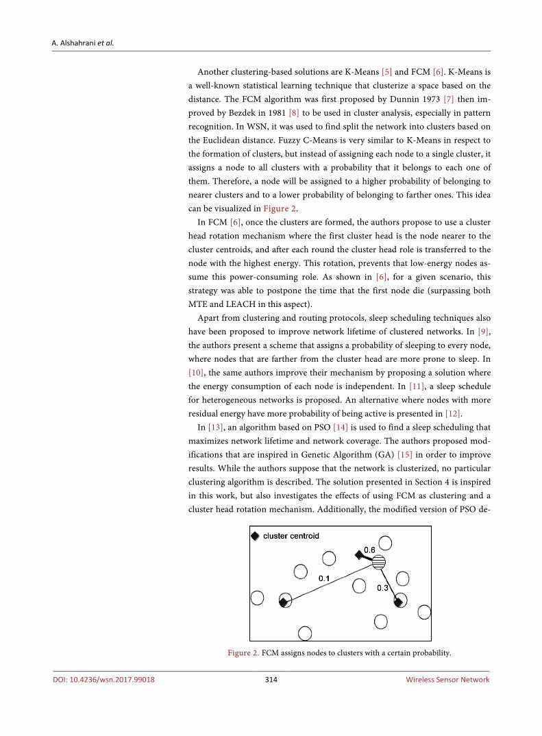
Another clustering-based solutions are K-Means [5] and FCM [6]. K-Means is a well-known statistical learning technique that clusterize a space based on the distance. The FCM algorithm was first proposed by Dunnin 1973 [7] then im-proved by Bezdek in 1981 [8] to be used in cluster analysis, especially in pattern recognition. In WSN, it was used to find split the network into clusters based on the Euclidean distance. Fuzzy C-Means is very similar to K-Means in respect to the formation of clusters, but instead of assigning each node to a single cluster, it assigns a node to all clusters with a probability that it belongs to each one of them. Therefore, a node will be assigned to a higher probability of belonging to nearer clusters and to a lower probability of belonging to farther ones. This idea can be visualized in Figure 2.

In FCM [6], once the clusters are formed, the authors propose to use a cluster head rotation mechanism where the first cluster head is the node nearer to the cluster centroids, and after each round the cluster head role is transferred to the node with the highest energy. This rotation, prevents that low-energy nodes as-sume this power-consuming role. As shown in [6], for a given scenario, this strategy was able to postpone the time that the first node die (surpassing both MTE and LEACH in this aspect).

Apart from clustering and routing protocols, sleep scheduling techniques also have been proposed to improve network lifetime of clustered networks. In [9], the authors present a scheme that assigns a probability of sleeping to every node, where nodes that are farther from the cluster head are more prone to sleep. In [10], the same authors improve their mechanism by proposing a solution where the energy consumption of each node is independent. In [11], a sleep schedule for heterogeneous networks is proposed. An alternative where nodes with more residual energy have more probability of being active is presented in [12].

In [13], an algorithm based on PSO [14] is used to find a sleep scheduling that maximizes network lifetime and network coverage. The authors proposed mod-ifications that are inspired in Genetic Algorithm (GA) [15] in order to improve results. While the authors suppose that the network is clusterized, no particular clustering algorithm is described. The solution presented in Section 4 is inspired in this work, but also investigates the effects of using FCM as clustering and a cluster head rotation mechanism. Additionally, the modified version of PSO de-

Figure 2. FCM assigns nodes to clusters with a certain probability.

A. Alshahrani et al.

DOI: 10.4236/wsn.2017.99018 315 Wireless Sensor Network

scribed in Section 4 presents differences to the one proposed in [13], including a reduced number of hyperparameters.

In [16], authors propose a hybrid solution that uses FCM to clusterize the network and the original binary PSO as sleep scheduling mechanism. Besides, authors suppose the presence of energy-harvesting nodes to serve as cluster heads, aiming at recharging the excess of energy spent by cluster heads. The re-sults shown in [16] show that this hybrid technique has benefits over LEACH-C [4] and C-FCM [6]. The solution presented in Section 4 differs from the one proposed in [16] in two aspects: it supposes the use of a modified PSO algorithm and it considers that all nodes have the same capabilities, i.e. there are no ener-gy-harvesting devices.

The main reasons to use modified PSO instead of the original PSO are in-spired by [13]. One of them is that original PSO has some well-known issues, for instance, premature stagnation. Besides that, we found out that in practice, original PSO always find solutions that lead to shorter network lifetimes than modified PSO, as shown in Section 5.

In [17], NSGA-II [18] (Non-Dominated Sorting Algorithm, version 2) is used to optimize the scheduling of sleep slots. NSGA-II is a multi-objective optimiza-tion algorithm based on GA. In Section 5, we show that FCMMPSO results are comparable to ECCA, but usually with a better coverage rate. Besides, the pro-posed solution allows for the user to choose how much to weight each objective, while in ECCA (as it is), the algorithm cannot prioritize one objective in detri-ment for another.

3. Preliminaries

In this section, the energy model and the coverage/overlapping definitions are briefly explained.

3.1. Energy Model

The energy model adopted in Section 4 is based on [1]. Nodes contains 1 or more sensors, a micro-controller, a transceiver and an energy source.

Regarding the energy model, the sensors are assumed to be passive, i.e. they do not consume energy, while the other components are all active. The total energy expenditure depends whether the node is ordinary or if it is a cluster head, since ordinary nodes transmit to the cluster head while cluster heads transmit to the base station. Also, cluster heads need to communicate with every cluster node, while ordinary nodes communicate only with the cluster head.

The transmitter model considers two components: the energy dissipated by the transmitter circuitry, which depends on the length l of the messages being communicated, and the energy dissipated by the power amplifier Epa, which de-pends on the length of the messages, on the distance to the other communicant and on the channel model. The total energy Etx is represented in Equation (1).

tx tx paE l Eξ= ∗ + (1)

A. Alshahrani et al.

DOI: 10.4236/wsn.2017.99018 316 Wireless Sensor Network

where ξtx is the energy per bit spent by the transmitter circuitry (50 nJ/bit). Two channel models are considered (based on [19]): free space with direct

line of sight and multipath fading one. The energy dissipated by the first one ( freespace

paE ) is shown in Equation (2) while the energy dissipated by the second one ( multipath

paE ) is shown in Equation (3): freespace 2pa fsE l dξ= ∗ ∗ (2)

multipath 4multipathpaE l dξ= ∗ ∗ (3)

where • ξfs is the energy per bit per square meter (with value 10 pJ/bit/m2), • ξmultipath is the energy per bit per quartic meter (with value 0.0013 pJ/bit/m4)

[20], • and d is the distance between communicants. d can be either the distance

from an ordinary node to the cluster head or the distance from the cluster head to the base station.

The choice of which model to use depends on the distance d. If d is less than d0 (described in Equation (4)), then the free space model is used, otherwise the chosen one is the multipath model.

freespace

0 multipathpa

pa

Ed

E= (4)

Additionally, cluster nodes shall take into account the energy dissipated while aggregating data from multiple nodes in the cluster (from a total of N nodes). This expenditure Eda is

da daE l Nξ= ∗ ∗ (5)

where ξda is 5 nJ/bit/message. The receiver model is simpler, it describes the energy dissipated at the receiver

circuitry, which depends on the message length and the number of messages m send to it (shown in Equation (6)):

rx rxE l mξ= ∗ ∗ (6)

where ξrx is the energy per bit spent by the receiver circuitry (50 nJ/bit). For or-dinary nodes, m is equal to 1 while for cluster heads m is equal to the number of the nodes in that cluster, minus one that is the cluster head itself.

The total energy dissipated in one round (when every node send data to the cluster head and it aggregates and transmits it to the base station) is:

( )1 1cC N

da rx txc nE E E

= =+ +∑ ∑ (7)

where C is the total number of clusters and Nc is the number of nodes in cluster c.

3.2. Coverage and Overlapping Area Definitions

The definitions of coverage and overlapping areas are similar to the ones found

A. Alshahrani et al.

DOI: 10.4236/wsn.2017.99018 317 Wireless Sensor Network

in [13], with minor differences: Every node covers a circular area with a predefined radius (dependent on the

sensor), i.e. the node can monitor that region of space. The union of all node’s areas is called network coverage area.

Areas that are monitored by more than one node (i.e. intersection regions) are accounted for overlapping. The union of all these areas is called network over-lapping area.

Areas that are covered exclusively by one node are called exclusive regions. Areas that are covered by more than one node are called overlapping regions. Coverage rate is the partial network coverage area of a particular configura-

tion (when only a subset of nodes are active) over the total network coverage area.

Overlapping rate is the partial network overlapping area of a particular confi-guration (when only a subset of nodes are active) over the total network over-lapping area.

Sleeping rate is the proportion of nodes that are sleeping (compared to all nodes).

These definitions apply to the entire network (when all nodes are active), but can also be calculated with a subset of the network’s members.

4. Methodology

The proposed solution consists of using FCM for clustering the network, then using a straightforward cluster head rotation mechanism in each round and scheduling sleep slots with the modified PSO, which maximizes both ener-gy-balance and network coverage. The clustering phase and cluster head rotation mechanism is described in Section 4.1 and the modified PSO is described in Sec-tion 4.2.

4.1. Clustering Phase

The first step required in clustering is to determine the optimal number of clus-ters. For this purpose, Equation (8) [16] is used:

22 πfs

mp toBS

EN MCE d

=∗

(8)

where: C is the number of clusters; N is the number of sensor nodes; Efs is the energy spent in the transmission of a single bit of data through free

space, achieving an acceptable bit error rate; Emp is the energy spent in the transmission of a single bit of data through a

multipath fading model, achieving an acceptable bit error rate; M is the network diameter; dtoBS is the average Euclidean distance from the cluster heads to the base sta-

tion.

A. Alshahrani et al.

DOI: 10.4236/wsn.2017.99018 318 Wireless Sensor Network

Notice also that Efs and Emp are dependent on the distance of transmission. Once the number of clusters is defined, the FCM algorithm helps to determine

both the cluster centroids and the initial assignment of sensor nodes to clusters. For that purpose, the method minimizes the following objective function (Equa-tion (9)):

21 1

, 1C N mm ij iji j

J u d m= =

= ≤ < ∞∑ ∑ (9)

where uij is the coefficient representing the degree of membership of the node i w.r.t. the cluster j, d is the Euclidean distance between the ith node and the jth cluster centroid, and m is a real parameter that represents the fuzzyness of the clusters. The uij coefficients form a coefficient matrix U where i indexes the ith row and j indexes the jth column.

The coefficients of the U matrix are calculated as follows (Equation (10)):

21

1

1ij

mC ijk

kj

udd

−

=

=

∑

(10)

where dkj is the Euclidean distance between the kth sensor node and the jth clus-ter centroid. Equation (10) shows that the greater the distance between a node and a centroid, the smaller the respective coefficient will be. The matrix U is in-itialized with random samples from a uniform distribution with values ranging from 0 to 1 (representing a probability).

The cluster centroids are iteratively calculated using Equation (11):

1

1

N mij ii

j N miji

u xc

u=

=

= ∑∑

(11)

where xi is the geolocation of the ith node and cj is the geolocation of the jth clus-ter centroid.

The complete algorithm is show in Algorithm 1. Lines 1 - 3 show the initiali-zation of the matrix U (U(0)). Lines 6 - 11 represent an iteration, where for each cluster the centroid is iteratively calculated using Equation (4) (line 9). The membership matrix is updated at each iteration using Equation (3) (line 10). Fi-nally, the FCM algorithm stops either when the error is below some threshold ε, or when the algorithm had run for a certain number of iterations.

After completing, the algorithm has defined the degree of membership of nodes. Then, each node is initially set to belong to the cluster that it has the highest degree of membership.

The base station initially selects the node nearest to each cluster centroid as the cluster head. However, the network hierarchy overloads cluster heads: they must relay messages from every cluster node to the base station. Thus, they ex-pend energy faster than ordinary nodes. For this reason, the cluster head selec-tion must be dynamic in order to prevent those nodes to extinguish their energy supplies and to balance the energy load.

A. Alshahrani et al.

DOI: 10.4236/wsn.2017.99018 319 Wireless Sensor Network

Algorithm 1. FCM algorithm for cluster formation.

1

2

3

4

5

6

7

8

9

10

11

for i = 0 to N

for j = 0 to C

uij(0) ~ uniform(0.0, 1.0)

k ← 0

repeat

k ← k + 1

for j = 0 to C

update cluster centroid cj using Equation (4)

update U(k) using Equation (3)

until ||U(k) – U(k-1)|| < ε

Therefore, after the first round, the current cluster head elects another node to

be the new cluster head. It chooses the node with the highest residual energy (this information is sent to the cluster head in every packet). This procedure is repeated every exchange of data, meaning that the cluster head role is reassigned periodically. It is also important to notice that the FCM algorithm is only used at the initial setup of the network. From that moment on, the partitions (clusters) are fixed while the cluster head changes dynamically.

The cluster head is responsible for allocating time slots when cluster members can transmit. This is implemented using a TDMA schedule. Regarding power consumption, cluster members activate their radio component only during their own slots, reducing the power consumption. Also, transmission power is opti-mized since the Euclidean distance between nodes and cluster head is minimized by the FCM algorithm. Additionally, energy is saved due to the fact that data ag-gregation and fusion is executed at the cluster head, which compresses the in-formation sent to the base station.

4.2. Sleep Scheduling

PSO [14] is a computational method that optimizes an objective function by searching the solution space simultaneously with multiple “probes”, aiming to improve the proposed solution iteratively. It is inspired by the social behavior of living being herds, where each “probe” is called particle and it represents a can-didate solution. Particles move through the solution space looking for a local op-tima with a certain velocity. At each iteration, each particle velocity is updated proportionally to the particle’s own inertia (algorithm’s parameter) but is also partially redirected to the local (particle’s) best known position and to the global (swarm’s) best known position. Therefore the particle movement (velocity) has three components: an inertial one, a personal one and a social one; simulating the herd’s behavior.

PSO has been successfully used in several domains such as [21] [22] [23] [24] [25]. Specifically in the WSN applications, PSO was introduced by Kulkarni et al.

A. Alshahrani et al.

DOI: 10.4236/wsn.2017.99018 320 Wireless Sensor Network

Algorithm 2. Modified PSO Algorithm.

1

2

3

4

5

6

7

8

9

10

11

12

13

14

15

16

17

18

19

20

for each cluster do

for i = 1 to P do

pi ←initialize_particle()

li ← pi

if i = 1 or fitness(li) > fitness(g) then

g ← li

for it = 1 to M do

for i = 1 to P do

rp, rg ~ uniform(0.0, 1.0)

pi ← mutation(pi, ω)

if rp < φp then

pi ← crossover(pi, li)

if rg < φg then

pi ← crossover(pi, g)

if fitness(pi) > fitness(li) then

li ← pi

if fitness(pi) > fitness(g) then

g ← pi

[26], who presented PSO and showed now to use it for energy-saving purposes.

Algorithm 2 describes the modified PSO used in this paper. It is based on [13], which is inspired itself in the Genetic Algorithm. For each cluster, a differ-ent set of particles is generated and each set searches to maximize the sleep scheduling for that cluster independently. Each particle has N dimensions, where N is the number of nodes in that cluster. Each dimension is binary, meaning that it has only to points: 0 (for active nodes) and 1 (for nodes that will be put to sleep). Every particle dimension is randomly initialized with 0 or 1 with equal probabilities (0.5) (line 3). Then the ith particle’s best position li is set to the particle’s initial configuration pi (line 4). Then the swarm’s best position g is set to the best initial position (lines 5 - 6). In order to decide which particle has the best configuration, the fitness function is used (described later on this sec-tion). P is the number of particles that simultaneously searches for the solution.

Lines 8 - 20 describe the search for the best sleep configuration. This proce-dure is repeated for a certain number of iterations (M), which is found out in practice. Then for each particle, three basic steps are repeated: mutation (line 11), crossover with the particle’s best position (line 13) and crossover with the swarm’s best position (line 15). In each step, particle and swarm’s best positions are updated when the new particle reached better results in terms of the fitness function (lines 17 - 20).

In the modified PSO, the number of particles P keeps unchanged, meaning

A. Alshahrani et al.

DOI: 10.4236/wsn.2017.99018 321 Wireless Sensor Network

that every particle is mutated and suffers crossover but no additional particles are generated during this process.

The mutation and crossover functions are inspired in GA and are described in Algorithm 3 and Algorithm 4. Both functions differ from the functions de-scribed in [13], because our results shown that we achieved better learning (of particles’ positions) with these changes. The mutation function changes some of the dimensions of a particle (which is called in GA, individual). The function traverses the individual genes and statistically flips (Boolean negation) ω percent of the genes. The mutation allows for the particle to “move” in the search space, assuming new configurations. Therefore, larger ω leads to greater movements.

The crossover function takes two particles (individuals) as input and the re-sulting individual has statistically half of genes from one individual and half from the other. Crossing over allows the particle to be attracted towards its best position or towards the swarm’s best position.

The fitness function that the modified PSO tries to maximize is described by Equation (12):

1 2fitness f fα β= ∗ + ∗ (12)

It is the weighted sum of two terms, with parameters α and β. The first term is a function of the remaining energy at devices and it is different from the energy- related term used in [13] because we found out that in some situations using that function makes the modified PSO find that the best configuration is to put all nodes to sleep. In order to avoid that, instead of minimizing the sum of energies

Algorithm 3. Mutation function.

1

2

3

4

5

6

Function mutation (individual, ω)

for g = 1 to G do

r1 ~ uniform(0.0, 1.0)

if r1 < ω then

flip(individualg)

return individual

Algorithm 4. Crossover function.

1

2

3

4

5

6

7

8

Function crossover (father, mother)

r1 ~ uniform(0.0, 1.0)

for g = 1 to G do

if r1 < 0.5 then

childg ← fatherg

else

childg ← motherg

return child

A. Alshahrani et al.

DOI: 10.4236/wsn.2017.99018 322 Wireless Sensor Network

of all wake nodes, Equation (12) maximizes the probability that nodes with above-average energy levels are kept awake, while nodes with below-average energy levels are put to sleep. This improves energy-balance inside the cluster. In Equation (13), Eg is the energy of the gth node, G is the number of nodes (genes in GA terminology), pi is the ith particle and E is the average energy in the alive nodes.

( ) ( ) ( )( )( ) ( ),

1

1 . min ,0

max ,0 min ,0

G Gi g g gg g

G Gg gg g

p E E E Ef

E E E E

− − − −=

− − −

∑ ∑∑ ∑

(13)

The second term is the fitness function is related to the coverage and the overlapping areas (as defined in Section 3) and it is described in Equation (13). Regionsexclusive are the exclusive regions for a particular particle p, and Cove-rageall are the coverage area (see Section 3) for all alive nodes. Differently from [13], we only have one term related to coverage and overlapping areas instead of two, reducing the number of the algorithm’s parameters. The value of f2 may range from 0 (when awake nodes represented in the particle have no exclusive area) and 1 (when all awake nodes cover areas that no other node covers). Maximizing f2 maximizes coverage area while reducing the overlapping at the same time. Therefore the nodes that have more overlapping are more prone to be sleeping.

( )exclusive2

all

RegionsCoverage

pf = (14)

α and β should sum to 1 and are chosen depending on how much one values the network lifetime (term 1) and coverage area (term 2).

The modified PSO (Algorithm 2) has 3 hyperparameters, ω, φg and φg. The learning strategy was implemented according to [2]:

( )max max min it Mω ω ω ω= − − ∗ (15)

1 1p it Mφ = − ∗ (16)

11gφ φ= − (17)

5. Results and Discussion

The settings common to all scenarios are described below (except when men-tioned differently).

The 2-dimensional field where 300 nodes are distributed is 250 × 250 m2 and the nodes are distributed using an independent uniform distribution for axis x and y. The base station is at (125, 125), i.e. the center of the field. The message length is 4000 bits plus a 150 bit header. The coverage radius for every node is 20 meters. The fuzzyness factor is equal to 2, and the number of clusters is usually calculated as 5. The initial energy at every node is 2 Joules. Other energy-related settings are mentioned in Section 3.

Regarding the modified PSO settings, the fitness function α is set to 0.5 and β

A. Alshahrani et al.

DOI: 10.4236/wsn.2017.99018 323 Wireless Sensor Network

to 0.5 by default. The maximum number of iterations for modified PSO is 100 and the number of particles is set to 20.

In all simulations, except for the Direct Communication setup, we considered that the base station must regularly broadcast routing/clustering information and sleep scheduling in order to every node know how to proceed in the next round. This forces nodes to spend at least the energy to receive this information (considering a 4150 bit message). Some authors consider that the cluster head perform this functionality while other authors do not consider this step in the energy consumption.

It is also important to note that the results shown in this section do not con-sider the initial energy spend in case nodes need to send their position to the base station. For the settings described above, this expenditure is equal to 0.303 Joules net or 0.001 Joules per node (in average).

5.1. Scenario: Cluster Formation

In this scenario, we show the cluster formation generated by the FCM algorithm (Figure 3). Nodes are represented as points and each color indicates a different cluster membership. Gray solid lines are the boundaries of each cluster. Red tri-angles represent the cluster centroids while the red cross represent the base sta-tion. As mentioned earlier, each node in FCM belong to all clusters with a cer-tain probability. In this plot, we assigned nodes to the most probable cluster.

5.2. Scenario: Network Lifetime

In this scenario, DC, MTE, LEACH, FCM, FCM plus original PSO and FCMMPSO are analyzed from the network lifetime perspective. The results are shown in Figure 4.

As expected using DC makes nodes farther from the base station deplete their batteries first, but nodes nearer to the base station outlive any other algorithm. When using LEACH, nodes tend to survive longer than DC ones. The cluster

Figure 3. FCM cluster formation.

A. Alshahrani et al.

DOI: 10.4236/wsn.2017.99018 324 Wireless Sensor Network

Figure 4. Number of alive nodes vs time (in rounds).

rotation mechanism used for LEACH randomly selects the next cluster head (as [1]). This mechanism does not take node’s remaining energy into account. For this reason it performs poorly.

On the other hand, FCM rotates the cluster head role between higher-energy nodes, what improves the network lifetime. Clusters deplete their energies as a whole, causing step descents in the number of alive nodes.

Concerning MTE, nodes nearer to the base station forward messages of all other nodes that are farther from the base station. Therefore, these nodes are overloaded and are depleted quickly. When these nodes are off, the farther nodes have to communicate directly to the base station, and due to the effort of trans-mitting over larger distances, also get their batteries depleted. As expected, FCM with original PSO perform better than other methods that rely only on cluster-ing. This is straightforward since original PSO decides that some nodes should occasionally sleep, saving their batteries.

As shown, FCMMPSO outperforms all other strategies. It seems that the modified PSO was able to always find solutions that lead to improved network lifetime. It is important to note that FCMMPSO performed better in all simula-tions that we run, but are not included here for lack of space. Also, the settings used in these comparisons were exactly the same (including values for α and β).

In order to detail the results shown in Figure 4, Table 1 shows the time when the first node depletes its battery and the time when 30% of the nodes die, re-spectively. Also we included results (for the same distribution/position of nodes) where the base station is decentralized at (125, −75), i.e. out of the map.

Figure 5 shows the map where the nodes are distributed. Red triangles represent the cluster centroids while the red cross represent the base station. Each area is colored according to the time (round) when the surrounding nodes get their batteries depleted. Dark areas represent nodes that die earlier, while light colors represent nodes that die later in the network lifetime. The base sta-

A. Alshahrani et al.

DOI: 10.4236/wsn.2017.99018 325 Wireless Sensor Network

Figure 5. Map with time of depletion for FCMMPSO.

Table 1. Round when first node die and when 30% of nodes die (for different algo-rithms).

Algorithm

Base station at:

(125, 125) (125, −75)

Number of depleted nodes:

1 30% 1 30%

DC 430 1685 11 97

MTE 29 312 28 141

LEACH 906 1585 459 1247

FCM 1943 2363 1500 1595

FCM+PSO 3088 3117 1872 1955

FCMMPSO 3422 3477 2033 2102

tion is at the center of the map i.e. at (125, 125).

Since the base station is at the center of the map, those nodes are the last to die (they spend less energy communicating with the base station). As it can be seen, most of the clusters die almost at the same time (have the same color in the map). This means that the network lifetime lasts longer but also that all nodes die approximately together.

5.3. Scenario: Coverage Rate

In this scenario, the effects of the proposed solution on coverage, overlapping and sleeping rates are analyzed. For that purpose, simulations take into account four sets of configurations: • 0.0 and β = 1.0 (only coverage area is optimized); • α = 0.25 and β = 0.75 (coverage should be prioritized over lifetime); • α and β equal to 0.5 (network lifetime and coverage area should be optimized

equally);

A. Alshahrani et al.

DOI: 10.4236/wsn.2017.99018 326 Wireless Sensor Network

Table 2. Coverage, overlapping and sleeping rates with different settings for FCMMPSO.

α β Coverage rate Overlapping rate

0.0 1.0 0.95 ± 0.01 0.25 ± 0.04

0.25 0.75 0.90 ± 0.03 0.23 ± 0.05

0.5 0.5 0.88 ± 0.04 0.42 ± 0.08

0.75 0.25 0.83 ± 0.05 0.45 ± 0.09

Table 3. Coverage, overlapping and sleeping rates with different settings for ECCA.

α β Coverage rate Overlapping rate

0.0 1.0 0.89 ± 0.06 0.14 ± 0.07

0.25 0.75 0.87 ± 0.03 0.27 ± 0.07

0.5 0.5 0.86 ± 0.05 0.42 ± 0.08

0.75 0.25 0.84 ± 0.04 0.45 ± 0.08

• α = 0.75 and β = 0.25 (lifetime is more important than coverage).

Results for FCMMPSO are shown in Table 2, while results regarding ECCA [17] are shown in Table 3. Every cell represents the average rate followed by the standard deviation (averaged during the network lifetime).

Results show that FCMMPSO always find better solutions concerning cover-age rate (in comparison to ECCA), reaching a maximum improvement of 6%. It is important to notice that ECCA is based on NSGA-II, which is a multi-objective approach, meaning that by default it does not learn solutions that improve one objective while get worse on the other objective. This imposes a constraint to the learning approach when one wants to prioritize one objective over another.

The overlapping rates of both approaches are similar, and both manage to re-duce it to only 25% when b = 1.0 (coverage is the only goal). It is important to notice that for ECCA, the sleeping rate decreases as α increases. This behavior is exactly the opposed to what is expected, since as a increases one would expect to have more sleeping nodes to extend network lifetime, not fewer. This anomaly can be explained due to the fact that NSGA-II does not consider α and β (it is not a multi-objective problem converted to single-objective by using a weighted sum).

Figure 6 shows the relation between coverage rate and number of active nodes. In this scenario, 100 nodes are used. For the higher coverage rate (0.9 to 1), FCMMPSO is more effective in covering more area with less active nodes than ECCA. It must be noticed that even if this result depends on the distribu-tion of the nodes in the map, all simulations showed that FCMMPSO always uses less nodes for the same coverage rate.

5.4. Scenario: Energy

In order to analyze the energy savings, five simulations were considered, with increasing levels of the hyperparameter α (and therefore decreasing levels of the

A. Alshahrani et al.

DOI: 10.4236/wsn.2017.99018 327 Wireless Sensor Network

Figure 6. Coverage rate vs number of active nodes.

Figure 7. Average Energy spent per round (in Joules).

hyperparameter β). Figure 7 shows that as α increases, the sleep scheduling manages to reduce the average energy spent at each round through more sleep-ing rate. Standard deviations for each scenario are not shown in Figure 7 be-cause we found extremely small deviations, meaning that during the network lifetime the energy consumption is approximately linear. This property may be used to forecast the time when the network will be totally depleted. Using this information, manual replacement/recharging of node can be anticipated.

5.5. Scenario: Modified PSO Learning

It is important to verify if the optimization algorithm used by the sleep scheduler improves the objective function when compared to random guesses (no optimi-zation at all), otherwise the use of the modified PSO would be unnecessary. Ad-ditionally, we show that modified PSO learns as fast and as much as other pro-posed solutions, but with less hyperparameters. Using less hyperparameters makes the configuration of the system used during deployment easier.

For that purpose, the same scenario described in Section 5.1 is used. Then the

A. Alshahrani et al.

DOI: 10.4236/wsn.2017.99018 328 Wireless Sensor Network

Table 4. Learned fitness value with different parameters (by term).

α β Average final global fitness value

term 1 term 2 total

0.5 0.5 0.8473 0.8298 0.8385

1.0 0.0 0.9825 0.5065 0.9825

0.0 1.0 0.5294 0.9085 0.9085

Table 5. Learning metrics for modified PSO and PSO with the initialization shown in [13].

Modified PSO EBSS-PSO [13]

Initial fitness 0.6290 0.6247

Final fitness 0.8567 0.8577

Learning (difference) 0.2277 0.233

modified PSO and the optimization algorithm proposed in [13] (also based on PSO) are simulated and compared. Table 4 shows the results of these simula-tions. All values shown in Table 2 represent the average of the fitness function during different rounds.

The “Initial fitness” row indicates the value of the fitness function at the in-itialization. For modified PSO, the initialization randomly guesses the positions of the individuals, while the optimization used in [13] initializes the positions accordingly to a sleep probability. The sleep probability used in [13] requires the configuration of two hyperparameters and that every node should know its dis-tance to the cluster head and the number of neighbors inside its sensor coverage radius. The “Final fitness” row indicates the value of the fitness function after the optimization has reached the limit of iterations.

As show in Table 5, the algorithms reach almost identical results, which means that: first, modified PSO is capable of learning as much as the optimiza-tion shown in [13], which is better than random guessing; and secondly, that the random initialization used by modified PSO (which is less complex than the one used in [13], i.e. no need to use sleep probability) suffices.

Figure 8 shows the learning curve obtained when executing modified PSO. Similar curves occur every round, since the optimization, and consequently the sleep scheduling, are ran at every round.

To illustrate that the modified PSO is able to favor either energy-balance (thus network lifetime) or coverage, simulations with different values for the parame-ters α and β were ran (where α and β are parameters of the fitness/objective function in Equation (12).

These results are shown in Table 6. When both terms (see definition in Equa-tion (12)) are equally weighted (first row in Table 2), the algorithm optimizes term 1 and term 2 approximately equally. When energy-balance (network life-time) is favored (α equals to 1.0), it maximizes term 1 (second row) while term 2 is maximized when coverage is the priority (β equals to 1.0).

A. Alshahrani et al.

DOI: 10.4236/wsn.2017.99018 329 Wireless Sensor Network

Figure 8. Learning curve observed for FCMMPSO.

Table 6. Effect of different aggregation costs on LEACH, MTE and FCM. The round when the first node dies and when 30% of nodes die is shown.

Algorithm

Cost (% of the transmitted message)

0% cost 50% cost 100% cost

1st 30% 1st 30% 1st 30%

LEACH 877 1824 730 1269 340 962

MTE 2146 3932 716 1758 20 333

FCM 1566 2346 1441 1530 1003 1169

5.6. Scenario: Costly Aggregation

Let us define aggregation as the act of routing nodes (nodes that forward mes-sages from the source node to the final destination) of compressing the informa-tion before sending it upstream. Aggregation may be performed by cluster heads in clusterized networks or by almost every node in the case of MTE. It can be achieved by removing redundant sensed information, or even by raw compres-sion techniques that may work on multiple messages at once but that would not work for single node messages.

In previous scenarios we assumed that aggregation has cost equal to zero, i.e. that forwarding messages adds no more bits to the message other than the bits send by the cluster head itself. This seems to be a common hypothesis [6]. How-ever, it may be expected that in some situations this hypothesis may not hold (when messages have low redundancy).

In this scenario, the effect of aggregation cost is analyzed. Table 6 shows the effect that three different aggregation costs have on the network lifetime. The round when the first node die and when 30% of the nodes die is considered. The aggregation costs are defined in terms of the percentage of the transmitted mes-sage, meaning that 0% cost indicates that there is no aggregation cost and 100%

A. Alshahrani et al.

DOI: 10.4236/wsn.2017.99018 330 Wireless Sensor Network

indicates that the message is entirely forwarded. As expected, increasing the aggregation cost reduces the network lifetime, in-

dependently of the algorithm used. However, aggregation cost affects some algo-rithms more than others. For instance, with no cost, networks that use MTE out-live FCM and LEACH networks. However, when the aggregation compresses only 50% of the received message, FCM networks live twice as much as MTE and LEACH networks. This means that aggregation cost deteriorates MTE more than it does with LEACH or FCM. As matter of fact, when the aggregation costs 100% of the received message, the first node of a MTE network dies at the 20th round.

These results justify the use of FCM as clustering algorithm instead of MTE.

6. Conclusion

We presented an alternative solution to improve network lifetime while max-imizing network coverage area. FCM is used for network clustering, by splitting the network in small subsets where transmission power is kept low. Additionally, each cluster has a head rotation mechanism that seeks to prevent low-energy nodes from communicating directly to the base station, resulting at a better energy-balance. On top of that, sleep slots are distributed among cluster nodes, in order to extend network lifetime. Better configurations of sleep schedules are found using the modified PSO algorithm that searches for both saving-energy and high-coverage rate configurations. Results show that, by correctly setting up PSO hyperparameters, the algorithm is able to learn better configurations and thus provide meet the specifications of applications with different goals.

References [1] Heinzelman, W., Chandrakasan, A. and Balakrishnan, H. (2000) Energy-Efficient

Communication Protocols for Wireless Sensor Networks. Proceedings of the 33rd Annual Hawaii International Conference on System Sciences, Hawaii, January 2000.

[2] Ettus, M. (1998) System Capacity, Latency, and Power Consumption in Multi-hop-Routed SS-CDMA Wireless Networks. Radio and Wireless Conference, August 1998, 55-58. https://doi.org/10.1109/RAWCON.1998.709135

[3] Hastie, T., Tibshirani, R. and Friedman, J. (2009) The Elements of Statistical Learn-ing: Data Mining, Inference, and Prediction. 2nd Edition, Springer Series in Statis-tics, Springer, New York.

[4] Dhawan, H. and Waraich, S. (2014) A Comparative Study on LEACH Routing Pro-tocol and Its Variants in Wireless Sensor Networks: A Survey. International Journal of Computer Applications, 95, 21-27. https://doi.org/10.5120/16614-6454

[5] Tan, L., Gong, Y. and Chen, G. (2008) A Balanced Parallel Clustering Protocol for Wireless Sensor Networks using K-Means Techniques, Hskip 1em plus 0.5em Mi-nus 0.4em. Proceedings of the 2nd International Conference on Sensor Technolo-gies and Applications, Cap Esterel, August 2008, 25-31.

[6] Hoang, D.C., Kumar, R. and Panda, S.K. (2010) Fuzzy C-Means Clustering Protocol for Wireless Sensor Networks. IEEE International Symposium on Industrial Elec-tronics, Bari, 3477-3482. https://doi.org/10.1109/ISIE.2010.5637779

A. Alshahrani et al.

DOI: 10.4236/wsn.2017.99018 331 Wireless Sensor Network

[7] Dunn, J.C. (1973) A Fuzzy Relative of the ISODATA Process and Its Use in Detect-ing Compact Well-Separated Clusters. Journal of Cybernetics, 3, 32-57. https://doi.org/10.1080/01969727308546046

[8] Bezdek, J.C. (1981) Pattern Recognition with Fuzzy Objective Function Algorithms. Plenum Press, New York. https://doi.org/10.1007/978-1-4757-0450-1

[9] Deng, J., Han, Y.S., Heinzelman, W.B. and Varshney, P.K. (2005) Scheduling Sleeping Nodes in High Density Cluster-Based Sensor Networks. Mobile Networks and Applications, 10, 825-835. https://doi.org/10.1007/s11036-005-4441-9

[10] Deng, J., Han, Y.S., Heinzelman, W.B. and Varshney, P.K. (2005) Balanced-Energy Sleep Scheduling Scheme for High Density Cluster-Based Sensor Networks. Elsevier Computer Communications Journal, 28, 1631-1642.

[11] Sekhar, S. (2005) A Distance Based Sleep Schedule Algorithm for Enhanced Life-time of Heterogeneous Wireless Sensor Networks. Master’s Thesis, University of Cincinnati.

[12] Pearlman, M.R., Deng, J., Liang, B. and Haas, Z.J. (2002) Elective Participation in Ad Hoc Networks Based on Energy Consumption. Proceedings of IEEE Global Tel-ecommunications Conference, November 2002, 26-31. https://doi.org/10.1109/GLOCOM.2002.1188035

[13] Yu, C., Guo, W. and Chen, G. (2012) Energy-Balanced Sleep Scheduling Based on Particle Swarm Optimization in Wireless Sensor Network. 26th International Paral-lel and Distributed Processing Symposium Workshops & PhD Forum, Shanghai, 1249-1255. https://doi.org/10.1109/IPDPSW.2012.154

[14] Kennedy, J. and Eberhart, R. (1995) Particle Swarm Optimization. Proceedings of IEEE International Conference on Neural Networks, Vol. 4, 1942-1948. https://doi.org/10.1109/ICNN.1995.488968

[15] Holland, J. (1992) Adaptation in Natural and Artificial Systems. MIT Press, Cam-bridge.

[16] Chelbi, S., Dhahri, H., Abdouli, M., Duvallet, C. and Bouaziz, R. (2016) A New Hy-brid Routing Protocol for Wireless Sensor Networks. International Journal of Ad Hoc and Ubituitous Computing.

[17] Jia, J., Chena, J., Changa, G. and Tan, Z. (2009) Energy Efficient Coverage Control in Wireless Sensor Networks Based on Multi-Objective Genetic Algorithm. Com-puters and Mathematics with Applications, 57, 1756-1766.

[18] Deb, K., Pratap, A., Agarwal, S. and Meyarivan, T. (2002) A Fast and Elitist Mul-tiobjective Genetic Algorithm: NSGA-II.in IEEE Transactions on Evolutionary Computation, 6, 182-197. https://doi.org/10.1109/4235.996017

[19] Rappaport, T. (1996) Wireless Communication: Principles and Practice. Prentice Hall, Englewood.

[20] Heinzelman, W.B., Chandrakasan, A.P. and Balakrishnan, H. (2002) An Applica-tion-Specific Protocol Architecture for Wireless Microsensor Networks. IEEE Transactions on Wireless Communications, 1, Article ID: 660670. https://doi.org/10.1109/TWC.2002.804190

[21] Den Bergh, F.V. (2002) An Analysis of Particle Swarm Optimizers. PhD Eng. The-sis, Department of Computer Science, University of Pretoria.

[22] Du, W.L. and Li, B. (2008) Multi-Strategy Ensemble Particle Swarm Optimization for Dynamic Optimization. Information Sciences, 78, 3096-3109.

[23] Naka, S., Genji, T., Yura, T. and Fukuyama, Y. (2003) A Hybridparticle Swarm Op-timization for Distribution State Estimation. IEEE Transactions on Power Systems,

A. Alshahrani et al.

DOI: 10.4236/wsn.2017.99018 332 Wireless Sensor Network

18, 60-68. https://doi.org/10.1109/TPWRS.2002.807051

[24] Lin, C.J., Chen, C.H. and Lin, C.T. (2009) A Hybrid of Cooperative Particle Swarm Optimization and Cultural Algorithm for Neural Fuzzy Networks and Its Prediction Applications. IEEE Transactions on Systems, Man, and Cybernetics—Part C: Ap-plications and Reviews, 39, 55-68. https://doi.org/10.1109/TSMCC.2008.2002333

[25] Zielinski, K., Weitkemper, P., Laur, R. and Kammeyer, K.D. (2009) Optimization of Power Allocation for Interference Cancellation with Particle Swarm Optimization. IEEE Transactions on Evolutionary Computation, 13, 128-150. https://doi.org/10.1109/TEVC.2008.920672

[26] Kulkarni, R.V. and Venayagamoorthy, G.K. (2011) Particle Swarm Optimization in Wireless-Sensor Networks: A Brief Survey. IEEE Transactions on Systems, Man, and Cybernetics—Part C, 41, 262-267.

Submit or recommend next manuscript to SCIRP and we will provide best service for you:

Accepting pre-submission inquiries through Email, Facebook, LinkedIn, Twitter, etc. A wide selection of journals (inclusive of 9 subjects, more than 200 journals) Providing 24-hour high-quality service User-friendly online submission system Fair and swift peer-review system Efficient typesetting and proofreading procedure Display of the result of downloads and visits, as well as the number of cited articles Maximum dissemination of your research work

Submit your manuscript at: http://papersubmission.scirp.org/ Or contact wsn@scirp.org