Sensor and Simulation Notes

Note 496

March 2005

A Conical Slot Antenna and Related Antennas Suitable for Use with an Aircraft with Inflatable Wings

W. Scott Bigelow and Everett G. Farr Farr Research, Inc.

Carl E. Baum and Dean I Lawry Air Force Research Laboratory

Directed Energy Directorate

Abstract Airborne UWB radar systems require receive antennas that can be printed or mounted onto an inflatable wing. Such antennas need to reach as low as VHF frequencies, and must be positioned to look to the side of the aircraft. To satisfy these requirements, a tapered slot antenna (TSA) looking off the wingtip has been proposed. However, a conventional TSA receives only horizontal polarization. Here, we describe a new form of TSA, the conical slot antenna (CSA), which exhibits vertical polarity above and below the horizon. To test the approach, we built and tested a 1/8th scale model of a CSA. We observed a clean impulse response with FWHM of less than 70 ps. The maximum gain for both polarizations is between 0 and 10 dBi from 4 to 12 GHz. The return loss, however, is higher than we would like over most of the frequency range. Finally, we discuss a number of alternative concepts for mounting antennas onto UAVs with inflatable wings. ________________________ This work was sponsored in part by the Air Force Office of Scientific Research, and in part by the Air Force Research Laboratory, Directed Energy Directorate.

CONTENTS Section Title Page

1. Introduction..............................................................................................................3

2. Scale Model UWB Conical Slot Antenna (CSA) ....................................................4

3. Time Domain Reflectometry (TDR) and Return Loss (S11) for the CSA ..............5

4. Impulse Response Measurements ............................................................................7

5. Other Antenna Concepts for Inflatable Wings.......................................................18

6. Concluding Remarks..............................................................................................23

References ................................................................................................................................23

2

1. Introduction

Airborne UWB radar systems require receive antennas that can be printed or mounted onto an inflatable wing. Examples of inflatable wings are shown in [1]. Antennas are needed that can reach as low as VHF frequencies, and these antennas must be positioned to look to the side of the aircraft. To satisfy these requirements, a tapered slot antenna (TSA) looking off the wingtip has been proposed. However, a conventional TSA receives only a horizontal polarization – it can not easily be configured to receive vertical polarization. It is well known that polarization diversity can add extra capability to radar, so we explore here how one might add a capability to include a second polarization. In another related effort, we have characterized TSAs, and that work will appear in a forthcoming note. To add a capability to receive vertical polarization, we propose using a conical slot antenna (CSA), which exhibits vertical polarity above and below the horizon. This antenna was first suggested by C. E. Baum in [2] as a limited-angle-of-incidence and limited-time magnetic sensor, but the concept should be applicable here as well. To test the approach, we built and tested a 1/8th scale model of a CSA. We intended to design for a “typical” wing dimension of 1.52 m (5 ft.) in length by 0.91 m (2 ft.) in width, and our model was 1/8th this size. We observed a clean impulse response with FWHM of less than 70 ps. The maximum gain for both polarizations is between 0 and 10 dBi from 4 to 12 GHz. The return loss, however, is higher than we would like over most of the frequency range. We begin with a description of the CSA, including its design principles. We then provide measurements of its return loss and antenna pattern. Finally, we discuss a number of alternative concepts for mounting antennas onto UAVs with inflatable wings.

3

2. Scale Model UWB Conical Slot Antenna (CSA)

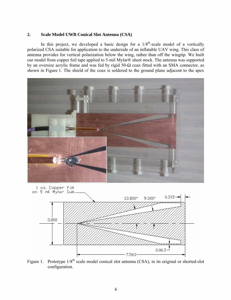
In this project, we developed a basic design for a 1/8th-scale model of a vertically polarized CSA suitable for application to the underside of an inflatable UAV wing. This class of antenna provides for vertical polarization below the wing, rather than off the wingtip. We built our model from copper foil tape applied to 5-mil Mylar® sheet stock. The antenna was supported by an oversize acrylic frame and was fed by rigid 50-Ω coax fitted with an SMA connector, as shown in Figure 1. The shield of the coax is soldered to the ground plane adjacent to the apex

Figure 1. Prototype 1/8th scale model conical slot antenna (CSA), in its original or shorted-slot

configuration.

4

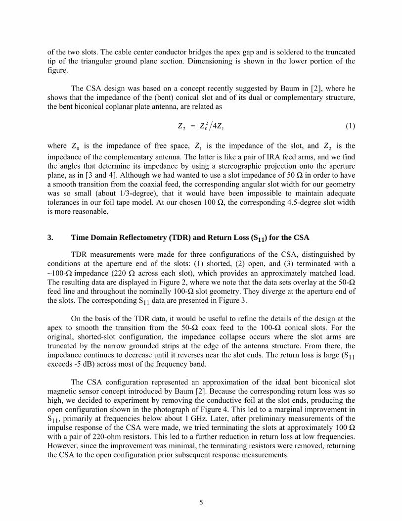
of the two slots. The cable center conductor bridges the apex gap and is soldered to the truncated tip of the triangular ground plane section. Dimensioning is shown in the lower portion of the figure. The CSA design was based on a concept recently suggested by Baum in [2], where he shows that the impedance of the (bent) conical slot and of its dual or complementary structure, the bent biconical coplanar plate antenna, are related as 1

202 4ZZZ = (1)

where is the impedance of free space, is the impedance of the slot, and is the impedance of the complementary antenna. The latter is like a pair of IRA feed arms, and we find the angles that determine its impedance by using a stereographic projection onto the aperture plane, as in [

0Z 1Z 2Z

3 and 4]. Although we had wanted to use a slot impedance of 50 Ω in order to have a smooth transition from the coaxial feed, the corresponding angular slot width for our geometry was so small (about 1/3-degree), that it would have been impossible to maintain adequate tolerances in our foil tape model. At our chosen 100 Ω, the corresponding 4.5-degree slot width is more reasonable.

3. Time Domain Reflectometry (TDR) and Return Loss (S11) for the CSA

TDR measurements were made for three configurations of the CSA, distinguished by conditions at the aperture end of the slots: (1) shorted, (2) open, and (3) terminated with a ~100-Ω impedance (220 Ω across each slot), which provides an approximately matched load. The resulting data are displayed in Figure 2, where we note that the data sets overlay at the 50-Ω feed line and throughout the nominally 100-Ω slot geometry. They diverge at the aperture end of the slots. The corresponding S11 data are presented in Figure 3. On the basis of the TDR data, it would be useful to refine the details of the design at the apex to smooth the transition from the 50-Ω coax feed to the 100-Ω conical slots. For the original, shorted-slot configuration, the impedance collapse occurs where the slot arms are truncated by the narrow grounded strips at the edge of the antenna structure. From there, the impedance continues to decrease until it reverses near the slot ends. The return loss is large (S11 exceeds -5 dB) across most of the frequency band. The CSA configuration represented an approximation of the ideal bent biconical slot magnetic sensor concept introduced by Baum [2]. Because the corresponding return loss was so high, we decided to experiment by removing the conductive foil at the slot ends, producing the open configuration shown in the photograph of Figure 4. This led to a marginal improvement in S11, primarily at frequencies below about 1 GHz. Later, after preliminary measurements of the impulse response of the CSA were made, we tried terminating the slots at approximately 100 Ω with a pair of 220-ohm resistors. This led to a further reduction in return loss at low frequencies. However, since the improvement was minimal, the terminating resistors were removed, returning the CSA to the open configuration prior subsequent response measurements.

5

0 2 4 6 8 10-0.5

0

0.5

1

TDR for CSA

Time (ns)

Ref

lect

ion

Coe

ffici

ent,

ρ

OpenTerminatedShorted

Figure 2. TDR measurements for three configurations of the CSA.

0 5 10 15 20-35

-30

-25

-20

-15

-10

-5

0S11 for CSA

Frequency (GHz)

|S11

(ω)|

(dB

)

OpenTerminatedShorted

100

101

-35

-30

-25

-20

-15

-10

-5

0S11 for CSA

Frequency (GHz)

|S11

(ω)|

(dB

)

OpenTerminatedShorted

Figure 3. Return loss measurements for three configurations of the CSA.

6

Figure 4. CSA in the open-slot configuration.

4. Impulse Response Measurements

4.1 Preliminary Response Measurements Our preliminary measurements of the impulse response behavior of the CSA were obtained on the PATAR® outdoor antenna range. This range includes a Picosecond Pulse Labs model 4015C step generator, a Tektronix model TDS8000 oscilloscope, and Farr Research model TEM-1-50 sensor and customized elevation/azimuth positioner and software. Subsequently, a more extensive set of measurements was obtained on our indoor range. We began our preliminary measurements by finding that the maximum response of the CSA to vertically polarized (normal to the plane of the antenna, or θ ) illumination occurs at zero degrees of azimuth and 17 degrees below the horizon (physical boresight). There, we recorded the impulse response in the time domain and calculated the corresponding realized gain, as shown in Figure 5. We observe a clean impulse, with a FWHM of 47 ps. The peak realized gain of about 8 dB occurs at 8.3 GHz. The frequency range over which the realized gain is above 0 dB is approximately 4 – 12 GHz. Since ours is a 1/8th-scale model, at full scale this frequency range corresponds to 0.5 – 1.5 GHz.

7

1 1.2 1.4 1.6 1.8 2-0.5

-0.4

-0.3

-0.2

-0.1

0

0.1

0.2CSA Response at (0,-17) θ - Polarization

Time (ns)

h N(t)

(m/n

s)

FWHM = 47 ps

0 5 10 15 20-35

-30

-25

-20

-15

-10

-5

0

5

10CSA Realized Gain at (0,-17) for θ - Polarization

Frequency (GHz)

Gr(ω

) (dB

i)

Figure 5. Normalized impulse response and realized gain of the open-slot CSA, at zero degrees

of azimuth and −17 degrees of elevation, with vertically polarized (θ ) illumination.

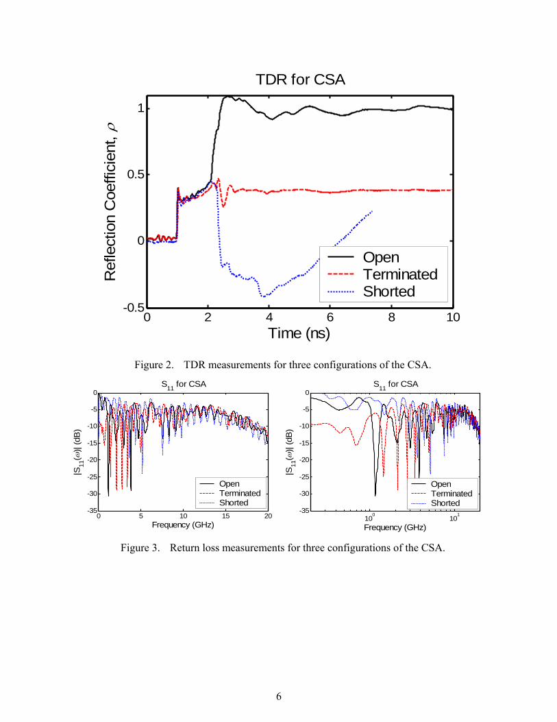
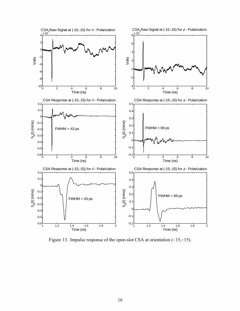
4.2 Response Pattern Measurements The CSA was originally conceived as a limited-angle-of-incidence, limited-time magnetic sensor for use in detecting the vertically (θ ) polarized electric field component scattered from a ground target. However, when the shorting strips were removed from the ends of the CSA slots, producing the open-slot configuration, the characteristics of the antenna were dramatically altered. Specifically, the antenna gained sensitivity to the horizontally (φ ) polarized electric field incident within the plane of the antenna (zero degrees of elevation) from directions off the end of each slot. The dual nature of the open-slot CSA motivated our characterization of the antenna pattern in certain key illumination planes for both horizontal and vertical polarizations. To characterize the CSA antenna, we have made pattern measurements on our indoor range by scanning, with both illumination polarizations, elevations from zero to −45 degrees at zero and −15 degrees of azimuth, and azimuths from zero to −45 degrees at zero and −15 degrees of elevation. The corresponding positive legs of these scans are available by symmetry. In the following sets of figures, we present both the pattern data and measurement data at individual key orientation coordinates. The key coordinates are those where relative sensitivity maxima occur, specifically, at (AZ,EL) = (φ,θ ) = (0,−15), (−15,0), and (−15,−15). We begin our characterization of the CSA by examining patterns for the peak normalized impulse response observed in the four planes, AZ = 0, AZ = −15, EL = 0, and EL = −15 degrees, as displayed in Figure 6. Corresponding patterns for realized gain as a function of frequency and angle are shown in Figure 7 and Figure 8. In examining the response data, we see that the vertical polarization component is null at zero degrees elevation, reaching a maximum at (0,−15). The horizontal component is null at zero degrees azimuth, reaching a maximum at (−15,0). At (−15,−15), while not at a maximum, the CSA is about equally sensitive to both polarization components. Physical boresight, (0,0), is a relative null for both components.

8

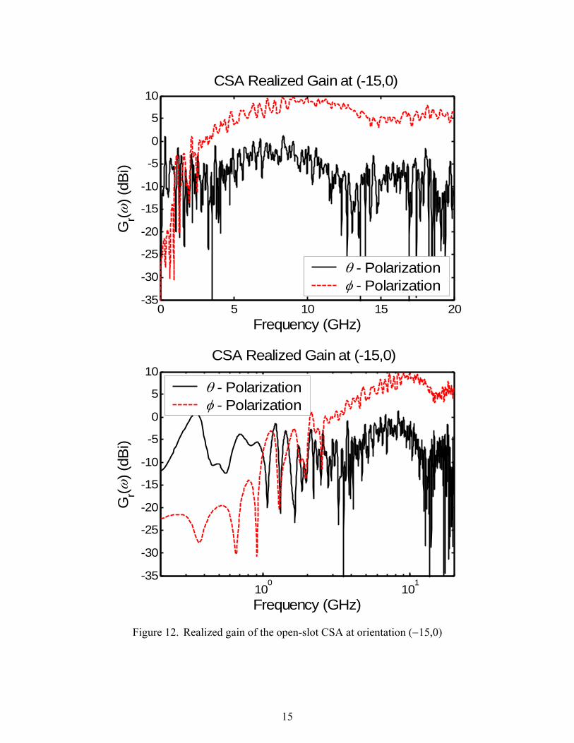
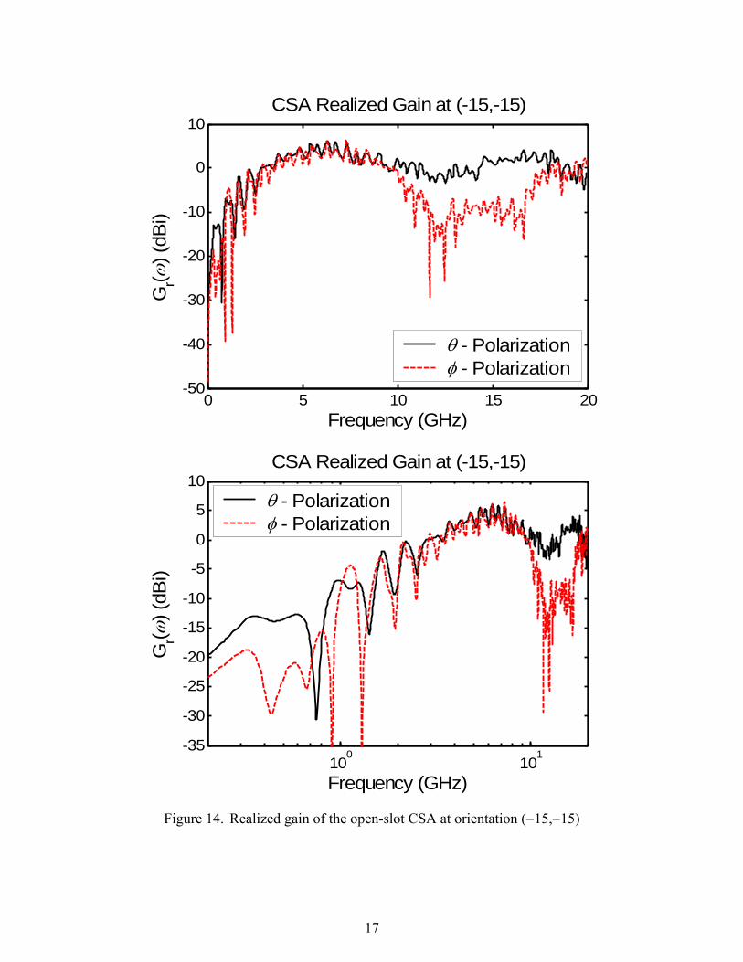
In Figure 9 and Figure 10, Figure 11 and Figure 12, and Figure 13 and Figure 14, we present data sets for the three key orientations identified above. Each set includes time domain response and realized gain for both vertical and horizontal polarizations.

0.2

0.4

0.6

0.8

30

210

60

240

90

270

120

300

150

330

180 0

Pattern for CSA

Peak hN(t) (m/ns) vs. Azimuth, EL = 0.0

θ - Polarizationφ - Polarization

0.1

0.2

0.3

0.4

0.5

30

210

60

240

90

270

120

300

150

330

180 0

Pattern for CSA

Peak hN(t) (m/ns) vs. Elevation, AZ = 0.0

θ - Polarizationφ - Polarization

0.1

0.2

0.3

0.4

0.5

30

210

60

240

90

270

120

300

150

330

180 0

Pattern for CSA

Peak hN(t) (m/ns) vs. Azimuth, EL = -15.0

θ - Polarizationφ - Polarization

0.2

0.4

0.6

0.8

30

210

60

240

90

270

120

300

150

330

180 0

Pattern for CSA

Peak hN(t) (m/ns) vs. Elevation, AZ = -15.0

θ - Polarizationφ - Polarization

Figure 6. Patterns for the peak normalized impulse response of the open-slot CSA.

9

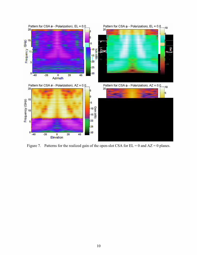
Figure 7. Patterns for the realized gain of the open-slot CSA for EL = 0 and AZ = 0 planes.

10

Figure 8. Patterns for the realized gain of the open-slot CSA for EL = 0 and AZ = 0 planes.

11

0 2 4 6 8 10-8

-6

-4

-2

0

2

4 x 10-3CSA Raw Signal at (0,-15) for θ - Polarization

Time (ns)

Vol

ts

0 2 4 6 8 10-1.5

-1

-0.5

0

0.5

1

1.5 x 10-3

CSA Raw Signal at (0,-15) for φ - Polarization

Time (ns)

Vol

ts

0 2 4 6 8 10-0.5

-0.4

-0.3

-0.2

-0.1

0

0.1

0.2CSA Response at (0,-15) for θ - Polarization

Time (ns)

h N(t)

(m/n

s)

FWHM = 63 ps

0 2 4 6 8 10-0.08

-0.06

-0.04

-0.02

0

0.02

0.04

0.06

0.08CSA Response at (0,-15) for φ - Polarization

Time (ns)

h N(t)

(m/n

s)

1 1.2 1.4 1.6 1.8 2-0.5

-0.4

-0.3

-0.2

-0.1

0

0.1

0.2CSA Response at (0,-15) for θ - Polarization

Time (ns)

h N(t)

(m/n

s)

FWHM = 63 ps

1 1.2 1.4 1.6 1.8 2-0.08

-0.06

-0.04

-0.02

0

0.02

0.04

0.06

0.08CSA Response at (0,-15) for φ - Polarization

Time (ns)

h N(t)

(m/n

s)

Figure 9. Impulse response of the open-slot CSA at orientation (0,−15).

12

0 5 10 15 20-35

-30

-25

-20

-15

-10

-5

0

5

10CSA Realized Gain at (0,-15)

Frequency (GHz)

Gr(ω

) (dB

i)

θ - Polarizationφ - Polarization

100

101

-35

-30

-25

-20

-15

-10

-5

0

5

10CSA Realized Gain at (0,-15)

Frequency (GHz)

Gr(ω

) (dB

i)

θ - Polarizationφ - Polarization

Figure 10. Realized gain of the open-slot CSA at orientation (0,−15).

13

0 2 4 6 8 10-3

-2

-1

0

1

2

3 x 10-3

CSA Raw Signal at (-15,0) for θ - Polarization

Time (ns)

Vol

ts

0 2 4 6 8 10-4

-2

0

2

4

6

8

10

12 x 10-3CSA Raw Signal at (-15,0) for φ -Polarization

Time (ns)

Vol

ts

0 2 4 6 8 10-0.2

-0.15

-0.1

-0.05

0

0.05

0.1

0.15CSA Response at (-15,0) for θ - Polarization

Time (ns)

h N(t)

(m/n

s)

0 2 4 6 8 10-0.4

-0.2

0

0.2

0.4

0.6

0.8

1CSA Response at (-15,0) for φ - Polarization

Time (ns)

h N(t)

(m/n

s)FWHM = 33 ps

1 1.2 1.4 1.6 1.8 2-0.2

-0.15

-0.1

-0.05

0

0.05

0.1

0.15CSA Response at (-15,0) for θ - Polarization

Time (ns)

h N(t)

(m/n

s)

1 1.2 1.4 1.6 1.8 2-0.4

-0.2

0

0.2

0.4

0.6

0.8

1CSA Response at (-15,0) for φ - Polarization

Time (ns)

h N(t)

(m/n

s)

FWHM = 33 ps

Figure 11. Impulse response of the open-slot CSA at orientation (−15,0).

14

0 5 10 15 20-35

-30

-25

-20

-15

-10

-5

0

5

10CSA Realized Gain at (-15,0)

Frequency (GHz)

Gr(ω

) (dB

i)

θ - Polarizationφ - Polarization

100

101

-35

-30

-25

-20

-15

-10

-5

0

5

10CSA Realized Gain at (-15,0)

Frequency (GHz)

Gr(ω

) (dB

i)

θ - Polarizationφ - Polarization

Figure 12. Realized gain of the open-slot CSA at orientation (−15,0)

15

0 2 4 6 8 10-10

-8

-6

-4

-2

0

2

4 x 10-3CSA Raw Signal at (-15,-15) for θ - Polarization

Time (ns)

Vol

ts

0 2 4 6 8 10-4

-2

0

2

4

6

8 x 10-3

CSA Raw Signal at (-15,-15) for φ - Polarization

Time (ns)

Vol

ts

0 2 4 6 8 10-0.6

-0.5

-0.4

-0.3

-0.2

-0.1

0

0.1

0.2CSA Response at (-15,-15) for θ - Polarization

Time (ns)

h N(t)

(m/n

s)

FWHM = 43 ps

0 2 4 6 8 10-0.2

-0.1

0

0.1

0.2

0.3

0.4

0.5CSA Response at (-15,-15) for φ - Polarization

Time (ns)

h N(t)

(m/n

s)FWHM = 69 ps

1 1.2 1.4 1.6 1.8 2-0.6

-0.5

-0.4

-0.3

-0.2

-0.1

0

0.1

0.2CSA Response at (-15,-15) for θ - Polarization

Time (ns)

h N(t)

(m/n

s)

FWHM = 43 ps

1 1.2 1.4 1.6 1.8 2-0.2

-0.1

0

0.1

0.2

0.3

0.4

0.5CSA Response at (-15,-15) for φ - Polarization

Time (ns)

h N(t)

(m/n

s)

FWHM = 69 ps

Figure 13. Impulse response of the open-slot CSA at orientation (−15,−15).

16

0 5 10 15 20-50

-40

-30

-20

-10

0

10CSA Realized Gain at (-15,-15)

Frequency (GHz)

Gr(ω

) (dB

i)

θ - Polarizationφ - Polarization

100

101

-35

-30

-25

-20

-15

-10

-5

0

5

10CSA Realized Gain at (-15,-15)

Frequency (GHz)

Gr(ω

) (dB

i)

θ - Polarizationφ - Polarization

Figure 14. Realized gain of the open-slot CSA at orientation (−15,−15)

17

5. Other Antenna Concepts for Inflatable Wings

Finally, we consider a number of related antenna concepts that may find use on an aircraft with inflatable wings. The work in this section extends the work previously presented in [5]. The simplest concept is the Tapered Slot Antenna (TSA). An example of such a device is shown in Figure 15, along with a possible mounting method. The width of the slot may be tapered in either a linear or spline shape, and examples of each are shown in Figure 16. Results on these devices will be published in a forthcoming note.

24

60

Printed Conductor

Tapered Slot

Figure 15. Full-scale tapered slot antenna (top, dimensions in inches), and a pair of tapered slot

antennas printed on aircraft wings (bottom).

Figure 16. Copper-foil-tape-on-Mylar® linear-taper slot antenna (F/M LTSA, left) and spline-

taper F/M STSA (right). Each antenna is mounted on an acrylic frame.

18

A number of other designs may be useful on inflatable wings on UAVs. The first of these is the four-strip pyramid, shown in Figure 17. When embedded into a wing, this can be configured to receive either horizontal or vertical polarization. However, this design has the disadvantage of requiring access to the interior of the wing. It would be preferable to have a design that can be painted or printed onto the wing after it has been built.

Figure 17. Four-strip pyramidal antenna.

The next configuration is the Maltese cross, printed onto the underside of a wing, as shown in Figure 18. This version receives both horizontal and vertical polarization. The component of vertical polarization is only that which is below the horizon. It should work well, but it does not take advantage of the entire length of the wing to achieve the maximum possible response at low frequencies.

Figure 18. Maltese cross antenna.

19

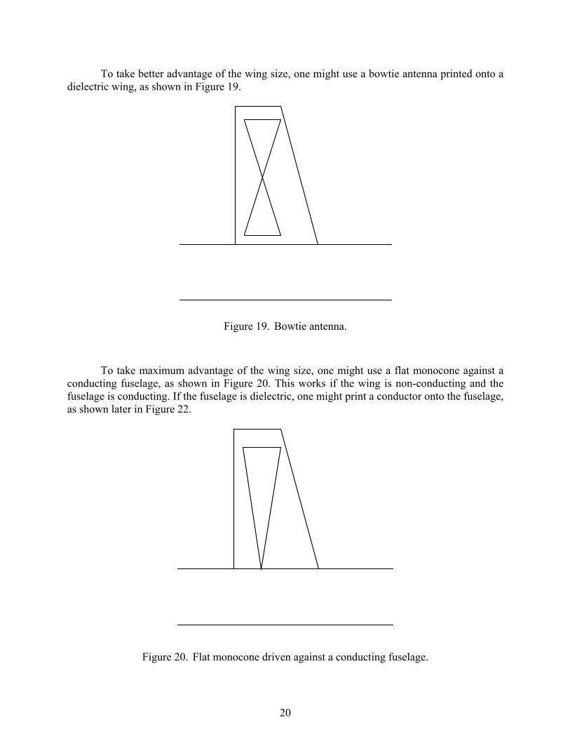
To take better advantage of the wing size, one might use a bowtie antenna printed onto a dielectric wing, as shown in Figure 19.

Figure 19. Bowtie antenna.

To take maximum advantage of the wing size, one might use a flat monocone against a conducting fuselage, as shown in Figure 20. This works if the wing is non-conducting and the fuselage is conducting. If the fuselage is dielectric, one might print a conductor onto the fuselage, as shown later in Figure 22.

Figure 20. Flat monocone driven against a conducting fuselage.

20

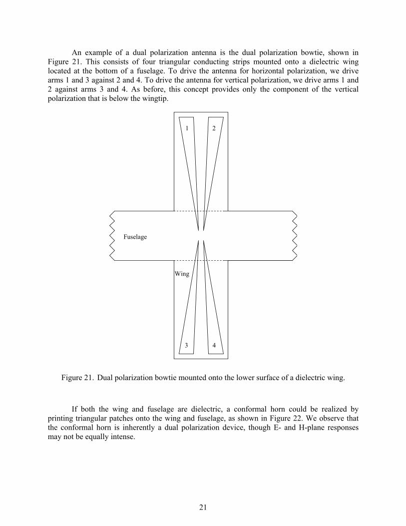
An example of a dual polarization antenna is the dual polarization bowtie, shown in Figure 21. This consists of four triangular conducting strips mounted onto a dielectric wing located at the bottom of a fuselage. To drive the antenna for horizontal polarization, we drive arms 1 and 3 against 2 and 4. To drive the antenna for vertical polarization, we drive arms 1 and 2 against arms 3 and 4. As before, this concept provides only the component of the vertical polarization that is below the wingtip.

1 2

3 4

Fuselage

Wing

Figure 21. Dual polarization bowtie mounted onto the lower surface of a dielectric wing.

If both the wing and fuselage are dielectric, a conformal horn could be realized by printing triangular patches onto the wing and fuselage, as shown in Figure 22. We observe that the conformal horn is inherently a dual polarization device, though E- and H-plane responses may not be equally intense.

21

DielectricFuselage

Dielectric Wing Conducting

Triangular Patches

Figure 22. Use of UAV geometry to form a conformal horn.

Finally, we note that the optimal vertical polarization may be obtained by printing a conducting monopole onto the vertical stabilizer of the UAV, as shown in Figure 23. This antenna can be driven against a conducting fuselage. If the fuselage is not conducting, a triangular patch can be printed onto it, as shown in Figure 22 for the conformal horn.

Fuselage (Conducting)

Vertical Stabilizer

(Dielectric)

ConductingMonopole

Figure 23. Vertical monopole mounted onto a dielectric vertical stabilizer.

22

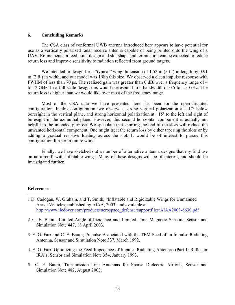
6. Concluding Remarks

The CSA class of conformal UWB antenna introduced here appears to have potential for use as a vertically polarized radar receive antenna capable of being printed onto the wing of a UAV. Refinements in feed point design and slot shape and termination can be expected to reduce return loss and improve sensitivity to radiation reflected from ground targets. We intended to design for a “typical” wing dimension of 1.52 m (5 ft.) in length by 0.91 m (2 ft.) in width, and our model was 1/8th this size. We observed a clean impulse response with FWHM of less than 70 ps. The realized gain was greater than 0 dBi over a frequency range of 4 to 12 GHz. In a full-scale design this would correspond to a bandwidth of 0.5 to 1.5 GHz. The return loss is higher than we would like over most of the frequency range. Most of the CSA data we have presented here has been for the open-circuited configuration. In this configuration, we observe a strong vertical polarization at ±17º below boresight in the vertical plane, and strong horizontal polarization at ±15º to the left and right of boresight in the azimuthal plane. However, this second horizontal component is actually not helpful to the intended purpose. We speculate that shorting the end of the slots will reduce the unwanted horizontal component. One might treat the return loss by either tapering the slots or by adding a gradual resistive loading across the slot. It would be of interest to pursue this configuration further in future work. Finally, we have sketched out a number of alternative antenna designs that my find use on an aircraft with inflatable wings. Many of these designs will be of interest, and should be investigated further. References 1 D. Cadogan, W. Graham, and T. Smith, “Inflatable and Rigidizable Wings for Unmanned

Aerial Vehicles, published by AIAA, 2003, and available at http://www.ilcdover.com/products/aerospace_defense/supportfiles/AIAA2003-6630.pdf

2. C. E. Baum, Limited-Angle-of-Incidence and Limited-Time Magnetic Sensors, Sensor and Simulation Note 447, 18 April 2003.

3. E. G. Farr and C. E. Baum, Prepulse Associated with the TEM Feed of an Impulse Radiating Antenna, Sensor and Simulation Note 337, March 1992.

4. E. G. Farr, Optimizing the Feed Impedance of Impulse Radiating Antennas (Part 1: Reflector IRA’s, Sensor and Simulation Note 354, January 1993.

5. C. E. Baum, Transmission–Line Antennas for Sparse Dielectric Airfoils, Sensor and Simulation Note 482, August 2003.

23