Embed Size (px)
DESCRIPTION
A Constant Factor Approximation Algorithm for the Multicommodity Rent-or-Buy Problem. Bell Labs CMU Cornell. Amit Kumar Anupam Gupta Tim Roughgarden. joint work with. The Rent-or-Buy Problem. t. t. 1. 2. s. s. 1. 2. Given source-sink pairs in a network. - PowerPoint PPT Presentation
Citation preview
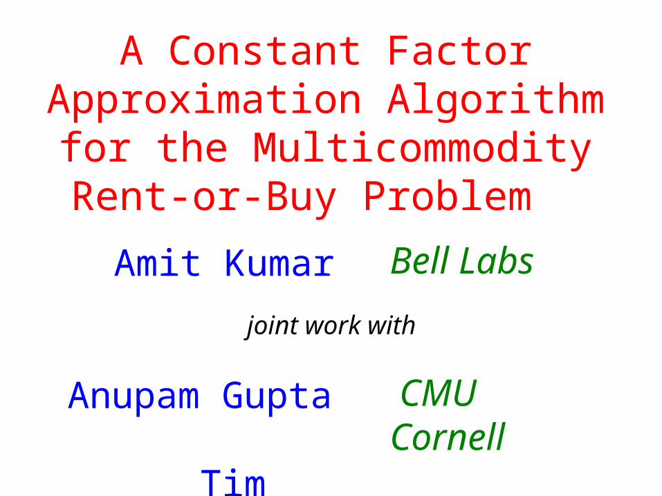
A Constant Factor Approximation Algorithm for the Multicommodity
Rent-or-Buy Problem
Amit Kumar
Anupam Gupta Tim Roughgarden
Bell Labs
CMUCornell
joint work with
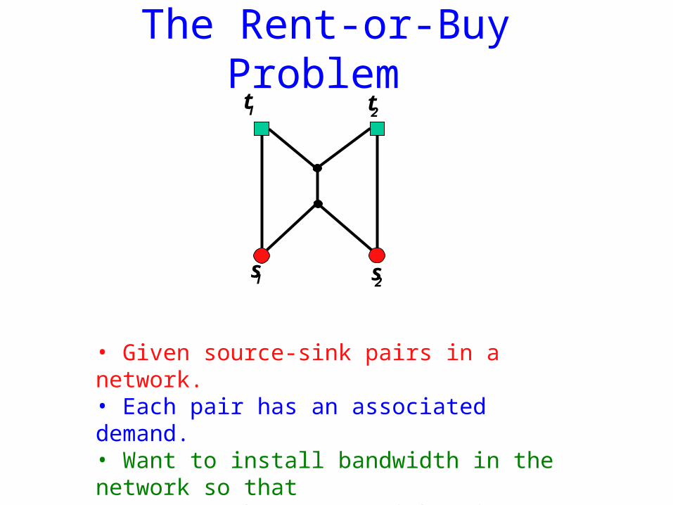
The Rent-or-Buy Problem
• Given source-sink pairs in a network. • Each pair has an associated demand. • Want to install bandwidth in the network so that the source-sink pairs can communicate.
t1 t2
s1 s2
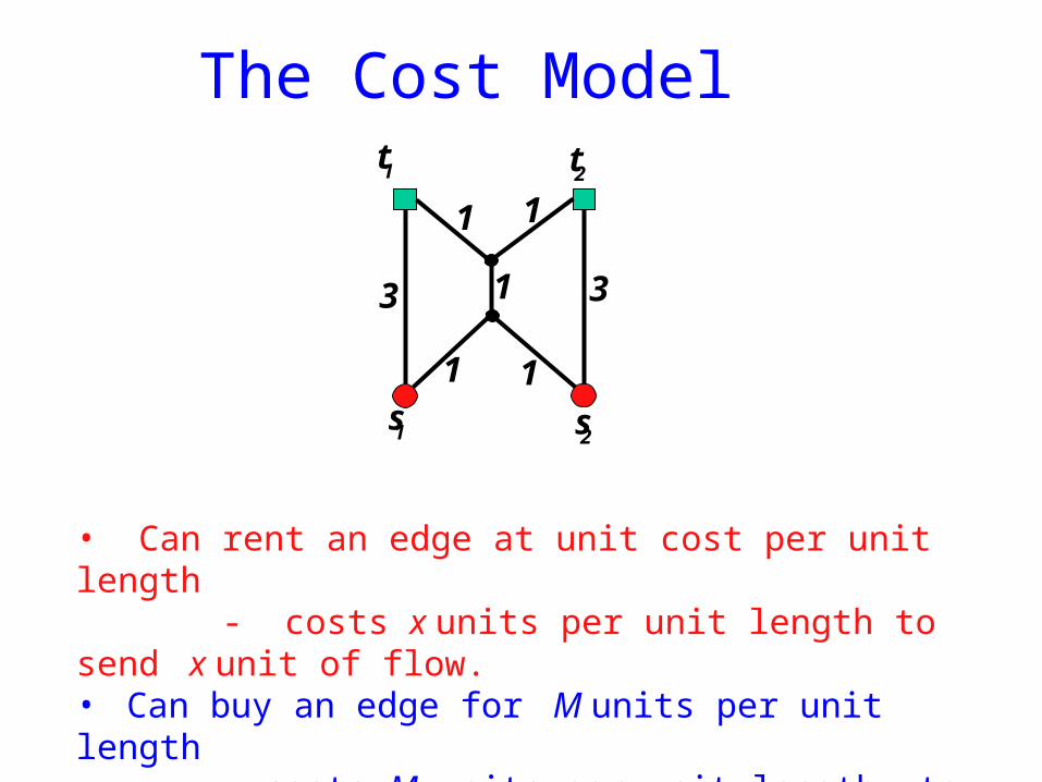
The Cost Model
• Can rent an edge at unit cost per unit length - costs x units per unit length to send x unit of flow.• Can buy an edge for M units per unit length - costs M units per unit length to send any amount of flow.
t1 t2
s1 s2
33
1
1
11
1

Example t1 t2
s1 s2
33
1
1
11
1t1 t2
s1 s2
33
1
1
11
1
M = 1.5
Cost = 6 Cost = 5.5
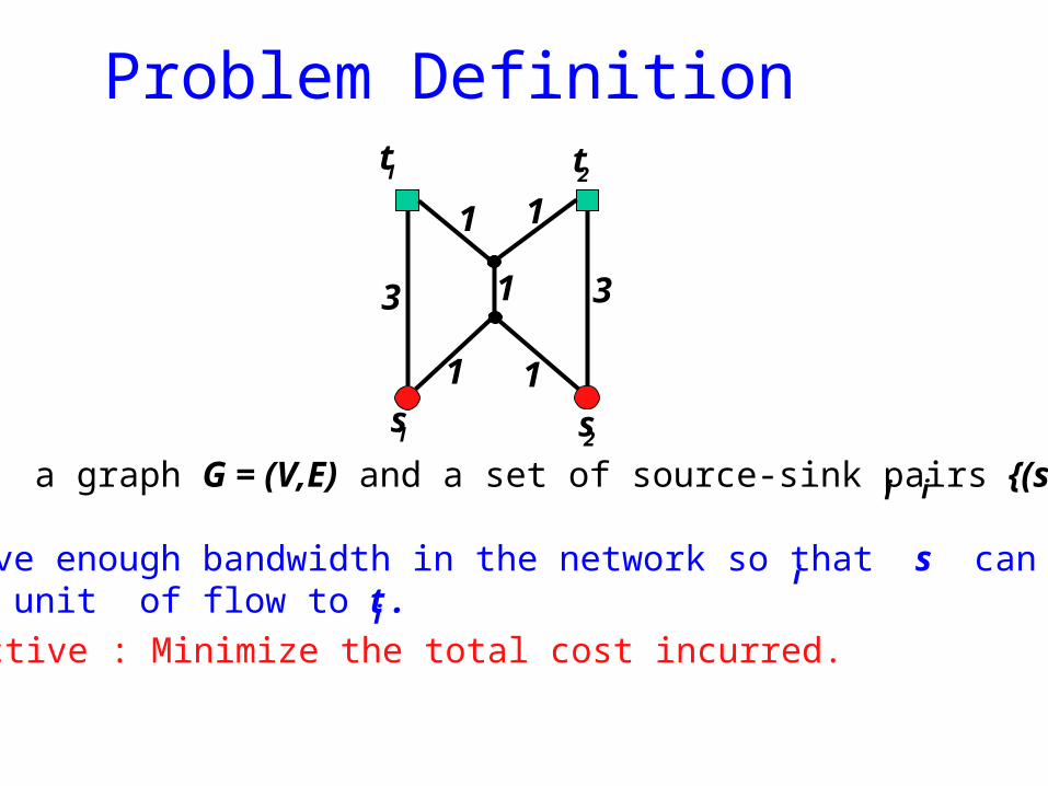
Problem Definition t1 t2
s1 s2
33
1
1
11
1
Given a graph G = (V,E) and a set of source-sink pairs {(s ,t )}.
Reserve enough bandwidth in the network so that s can send one unit of flow to t .
Objective : Minimize the total cost incurred.
ii
i
i
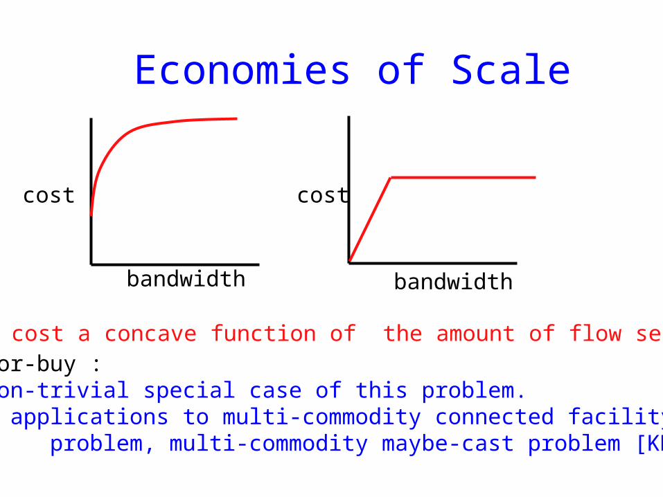
Economies of Scale
Edge cost a concave function of the amount of flow sent. Rent-or-buy : • a non-trivial special case of this problem. • has applications to multi-commodity connected facility location problem, multi-commodity maybe-cast problem [KM ’00].
bandwidth
cost
bandwidth
cost
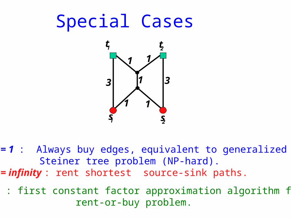
Special Cases t1 t2
s1 s2
33
1
1
11
1
• M = 1 : Always buy edges, equivalent to generalized Steiner tree problem (NP-hard).
• M = infinity : rent shortest source-sink paths.
Our result : first constant factor approximation algorithm for the rent-or-buy problem.
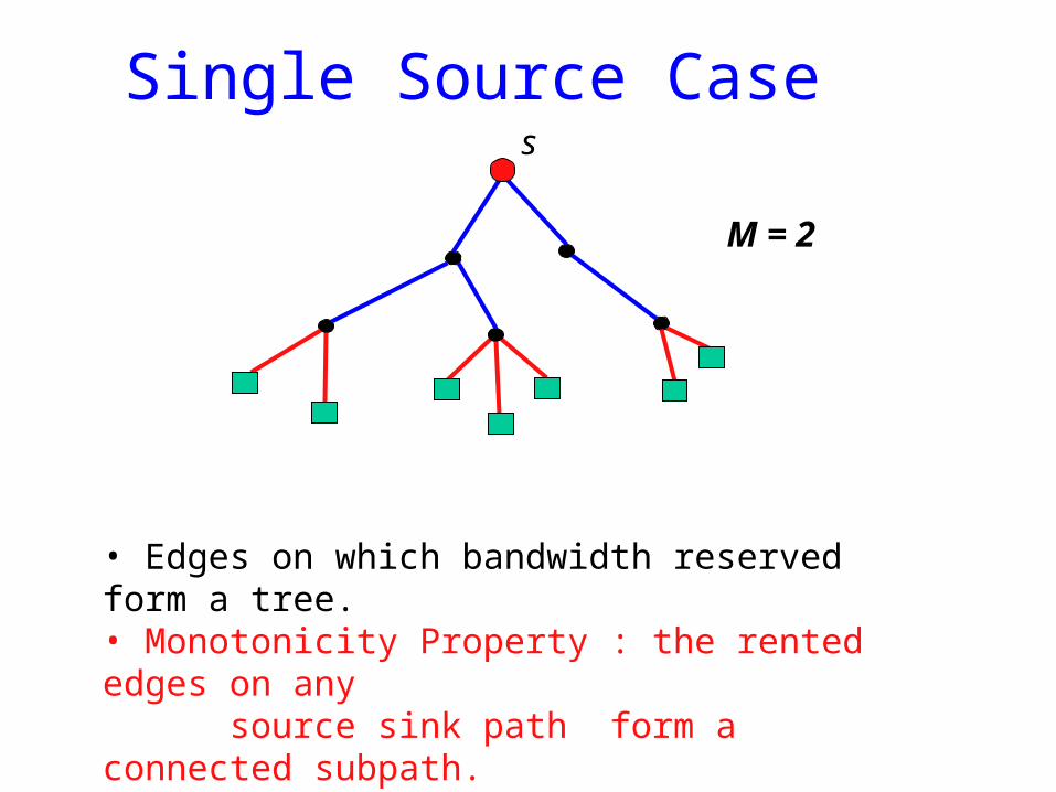
Single Source Case s
• Edges on which bandwidth reserved form a tree. • Monotonicity Property : the rented edges on any source sink path form a connected subpath.
M = 2
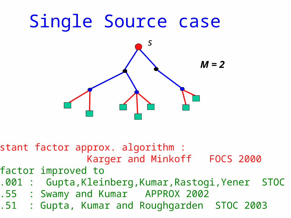
Single Source case s
M = 2
First constant factor approx. algorithm : Karger and Minkoff FOCS 2000Constant factor improved to 9.001 : Gupta,Kleinberg,Kumar,Rastogi,Yener STOC 2001 4.55 : Swamy and Kumar APPROX 2002 3.51 : Gupta, Kumar and Roughgarden STOC 2003
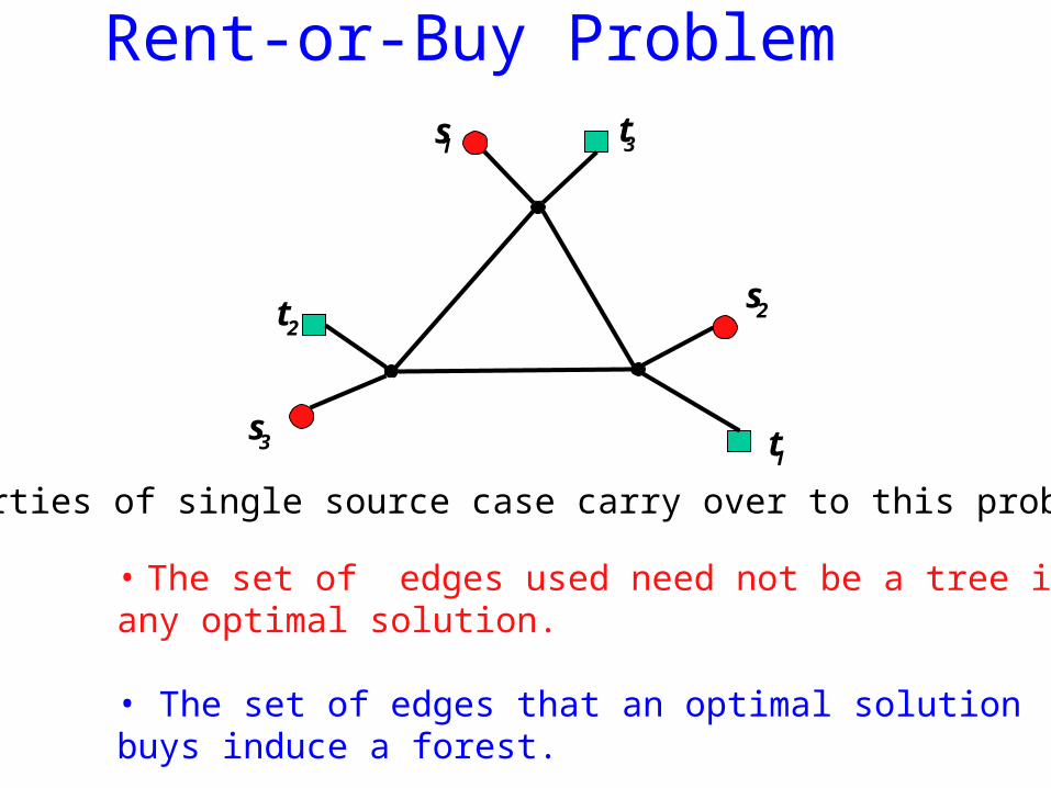
Rent-or-Buy Problem s1
s 2
s 3 t1
t 2
t3
What properties of single source case carry over to this problem ?
• The set of edges used need not be a tree in any optimal solution.
• The set of edges that an optimal solution buys induce a forest.
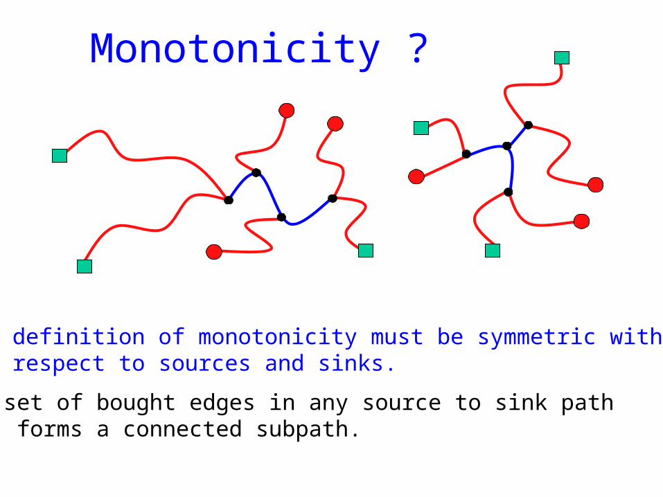
Monotonicity ?
The set of bought edges in any source to sink path forms a connected subpath.
The definition of monotonicity must be symmetric with respect to sources and sinks.
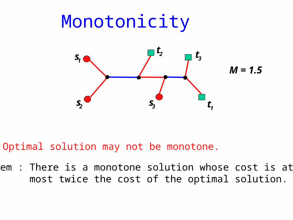
Monotonicity
t 3t 2
t 1s 3s 2
s 1M = 1.5
Theorem : There is a monotone solution whose cost is at most twice the cost of the optimal solution.
Optimal solution may not be monotone.
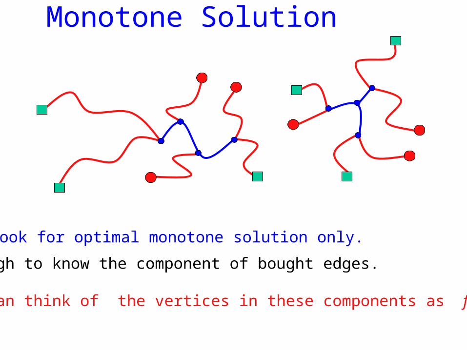
Monotone Solution
Look for optimal monotone solution only.
Enough to know the component of bought edges.
We can think of the vertices in these components as facilities.
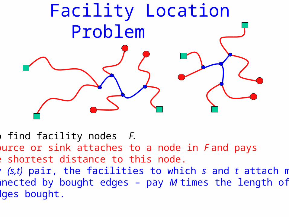
Facility Location Problem
Want to find facility nodes F. Each source or sink attaches to a node in F and pays the shortest distance to this node. For any (s,t) pair, the facilities to which s and t attach must be connected by bought edges – pay M times the length of edges bought.
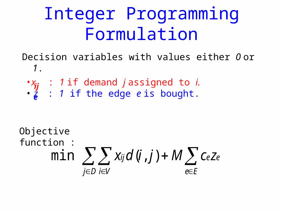
Integer Programming Formulation
Decision variables with values either 0 or 1.
•x : 1 if demand j assigned to i.• z : 1 if the edge e is bought.
ij
e
Objective function :
Ee
ee
Dj Vi
ij zcMjidx ),(min
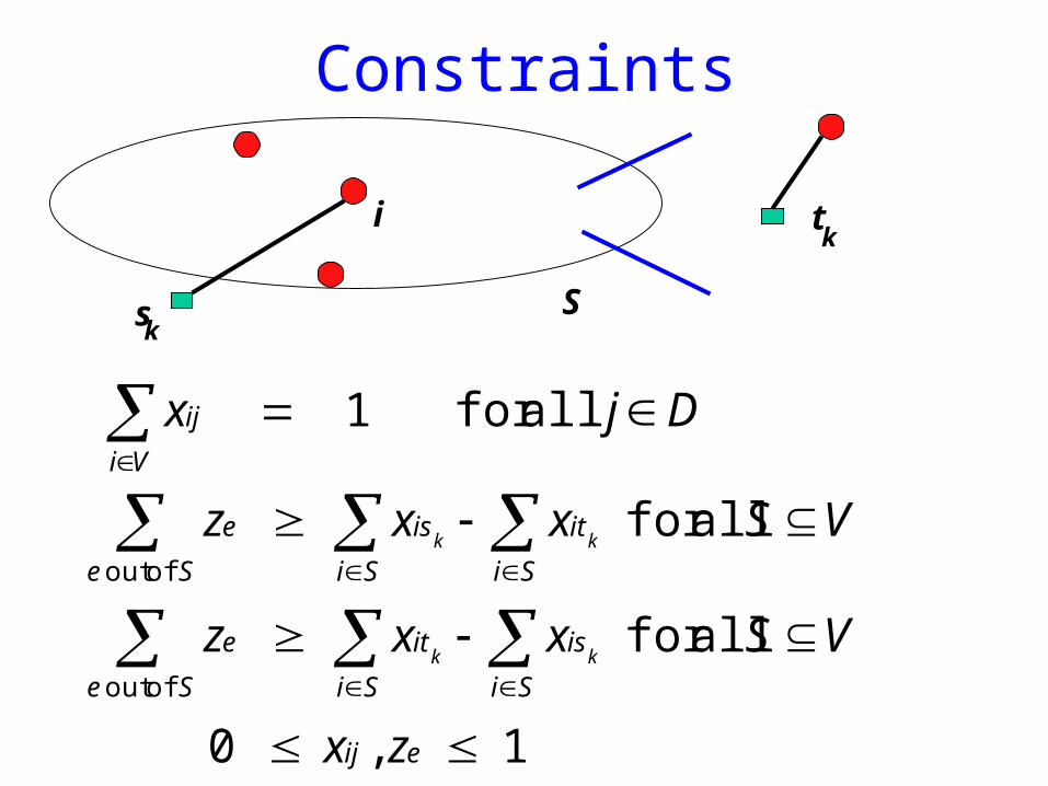
Constraints
1,0
allfor
allfor
allfor 1
ofout
ofout
eij
Se Si
is
Si
ite
Se Si
it
Si
ise
Vi
ij
zx
VSxxz
VSxxz
Djx
kk
kk
s
i
S
t
k
k
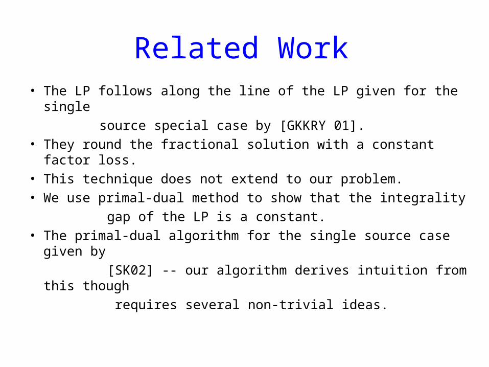
Related Work• The LP follows along the line of the LP given for the single
source special case by [GKKRY 01].
• They round the fractional solution with a constant factor loss.
• This technique does not extend to our problem.
• We use primal-dual method to show that the integrality
gap of the LP is a constant.
• The primal-dual algorithm for the single source case given by
[SK02] -- our algorithm derives intuition from this though
requires several non-trivial ideas.
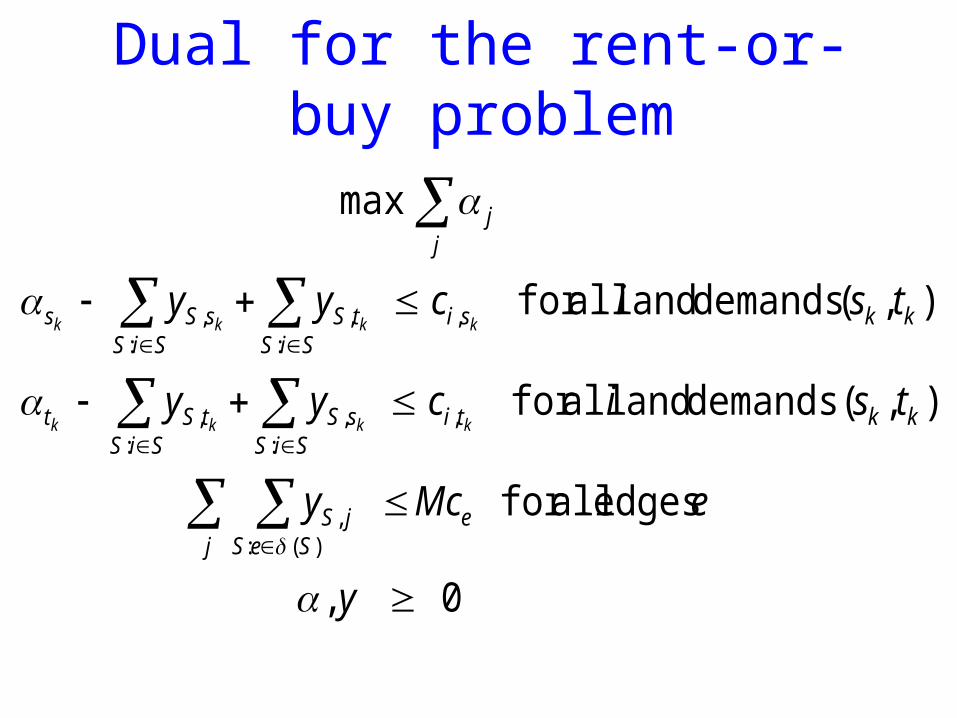
Dual for the rent-or-buy problem
0,
edges allfor
),( demands andallfor
),( demands and allfor
max
)(:,
,:
,:
,
,:
,:
,
y
eMcy
ts i cyy
tsicyy
ej SeS
jS
kktiSiS
sSSiS
tSt
kksiSiS
tSSiS
sSs
jj
kkkk
kkkk
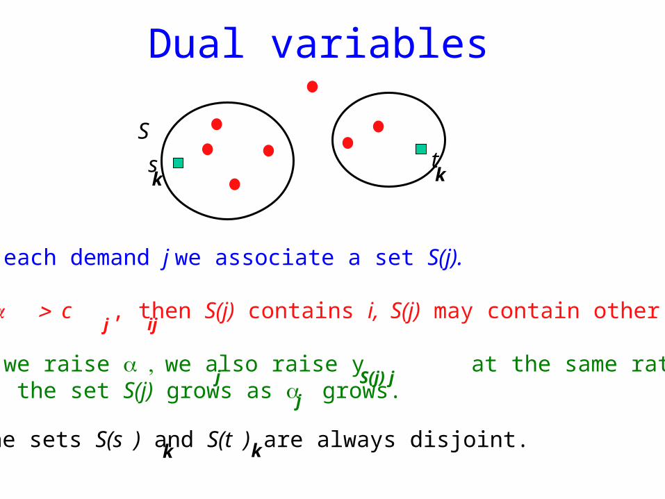
For each demand j we associate a set S(j).
If c , then S(j) contains i, S(j) may contain other nodes .
When we raise we also raise y at the same rate. the set S(j) grows as grows.
Dual variables
S
j ij
S(j) j
j
j
sk
tk
The sets S(s ) and S(t ) are always disjoint. k k
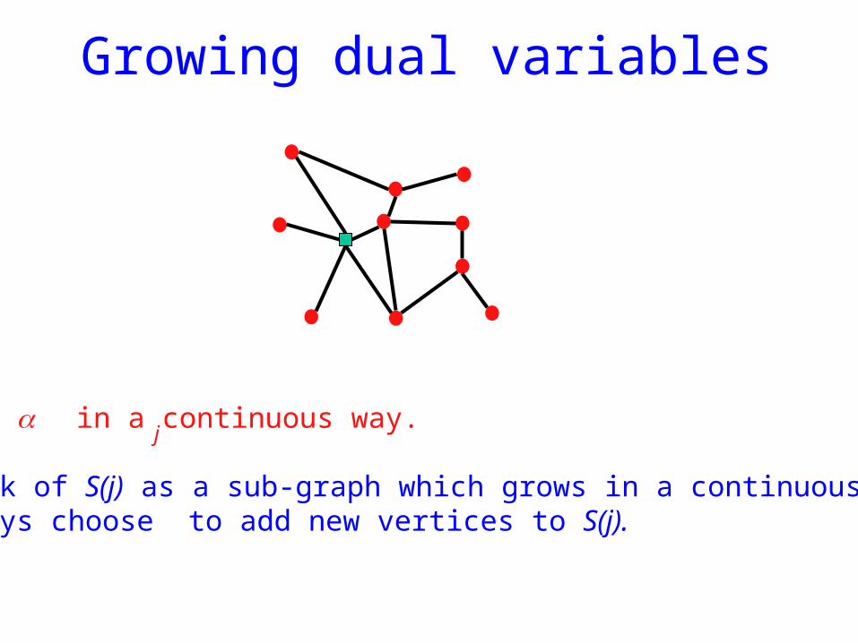
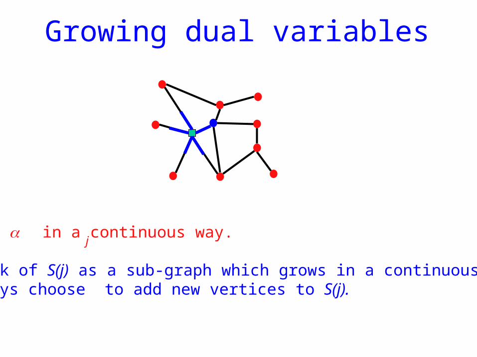
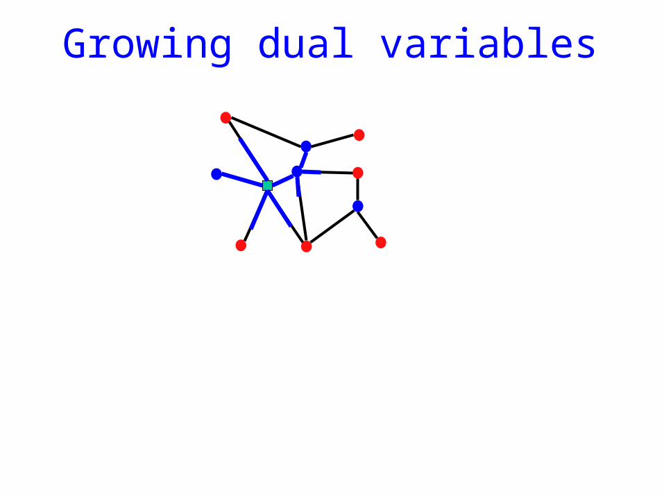
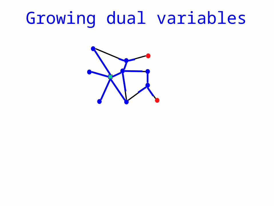
Growing dual variables
We raise in a continuous way.
Can think of S(j) as a sub-graph which grows in a continuous way. Can always choose to add new vertices to S(j).
j
Growing dual variables
We raise in a continuous way.
Can think of S(j) as a sub-graph which grows in a continuous way. Can always choose to add new vertices to S(j).
j
Growing dual variables
Growing dual variables
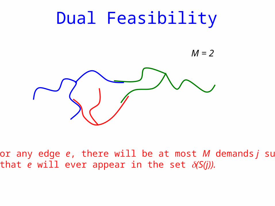
Dual Feasibility
M = 2
For any edge e, there will be at most M demands j such that e will ever appear in the set (S(j)).
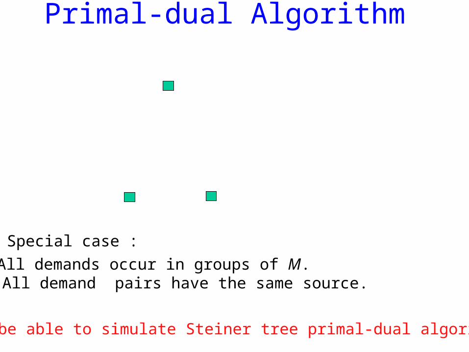
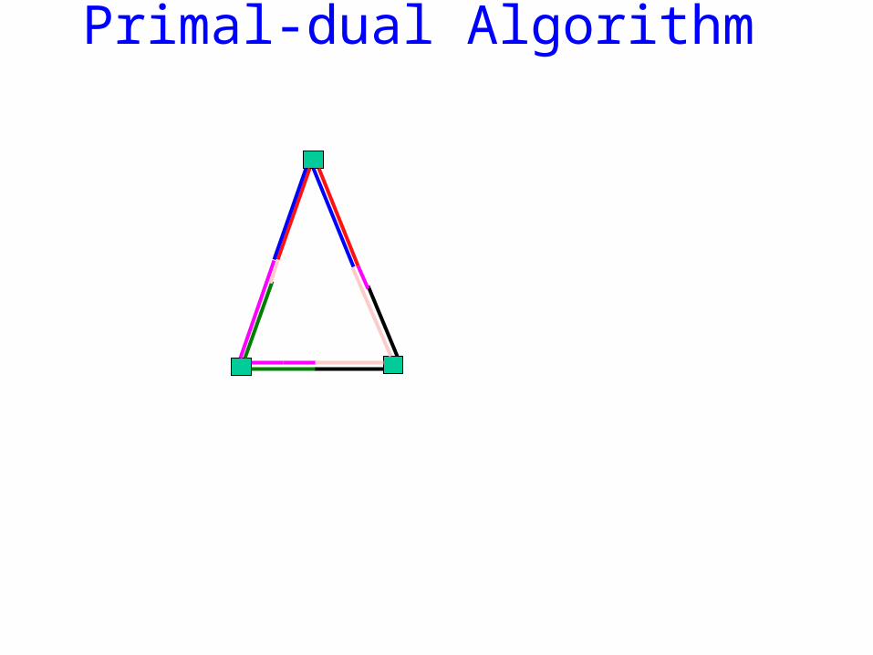
Primal-dual Algorithm
• All demands occur in groups of M. • All demand pairs have the same source.
Special case :
Should be able to simulate Steiner tree primal-dual algorithm.
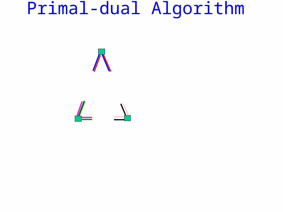
Primal-dual Algorithm
Primal-dual Algorithm
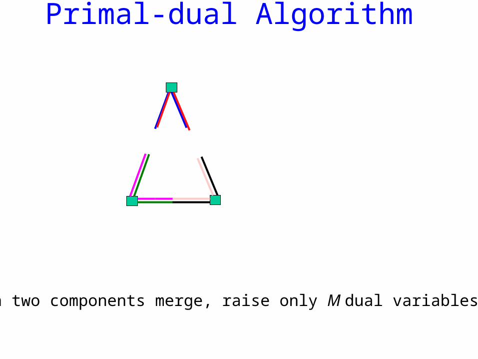
When two components merge, raise only M dual variables in it.
Primal-dual Algorithm
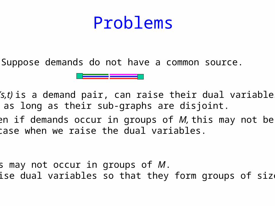
Problems
If (s,t) is a demand pair, can raise their dual variables as long as their sub-graphs are disjoint.
Even if demands occur in groups of M, this may not be the case when we raise the dual variables.
• Suppose demands do not have a common source.
• Demands may not occur in groups of M. – raise dual variables so that they form groups of size M.
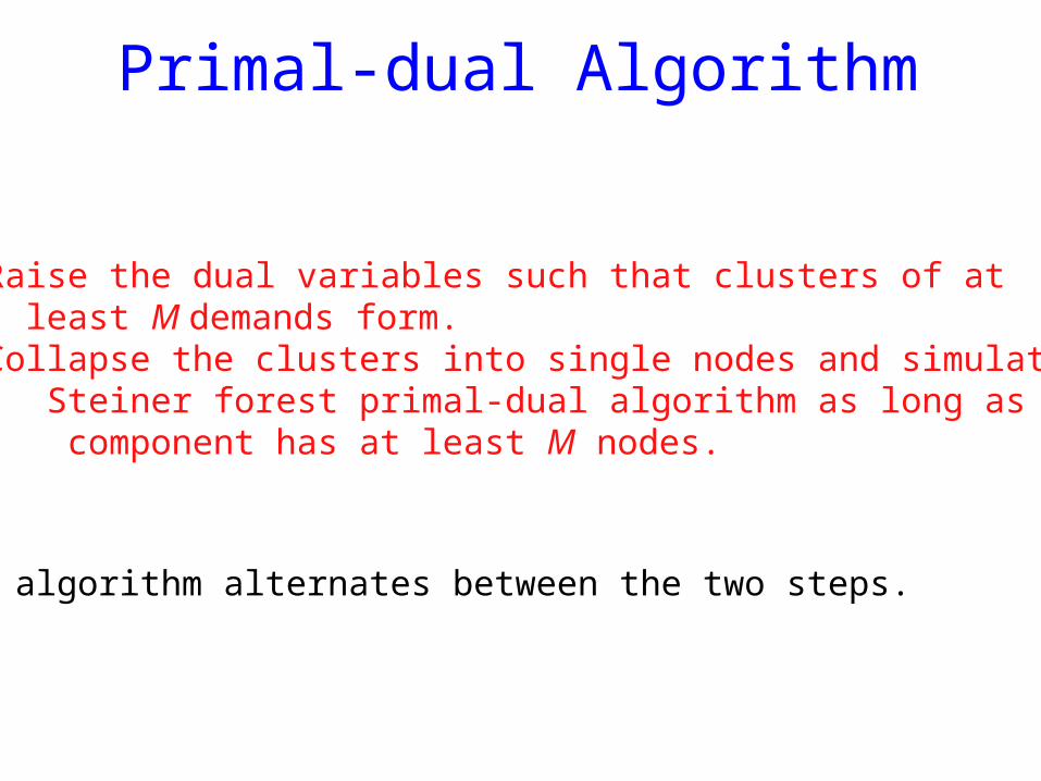
Primal-dual Algorithm
• Raise the dual variables such that clusters of at least M demands form.• Collapse the clusters into single nodes and simulate the Steiner forest primal-dual algorithm as long as each component has at least M nodes.
The algorithm alternates between the two steps.
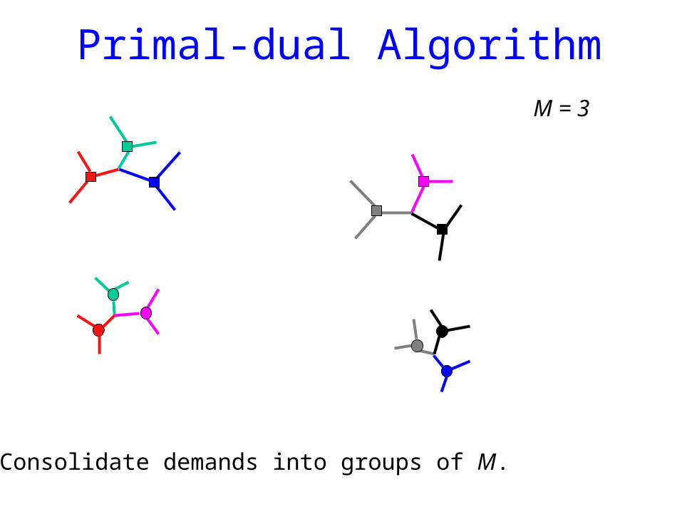
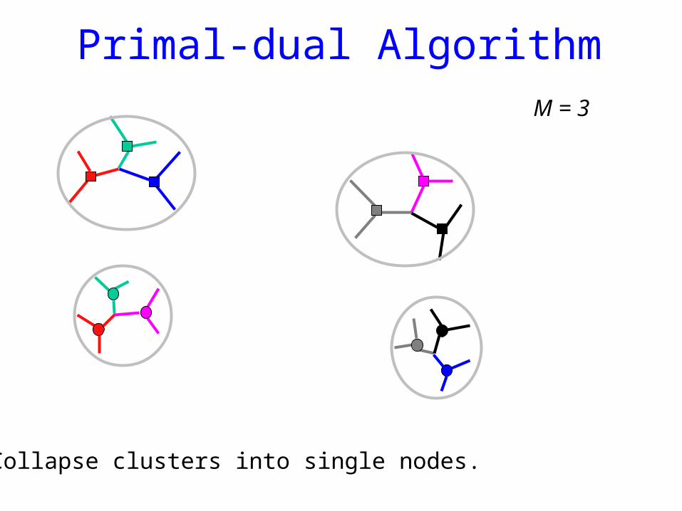
Primal-dual AlgorithmM = 3
Consolidate demands into groups of M.
Primal-dual AlgorithmM = 3
Collapse clusters into single nodes.
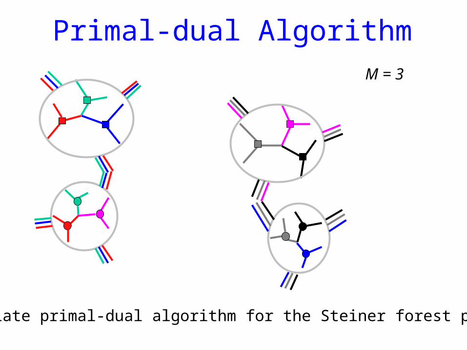
Primal-dual AlgorithmM = 3
Simulate primal-dual algorithm for the Steiner forest problem.
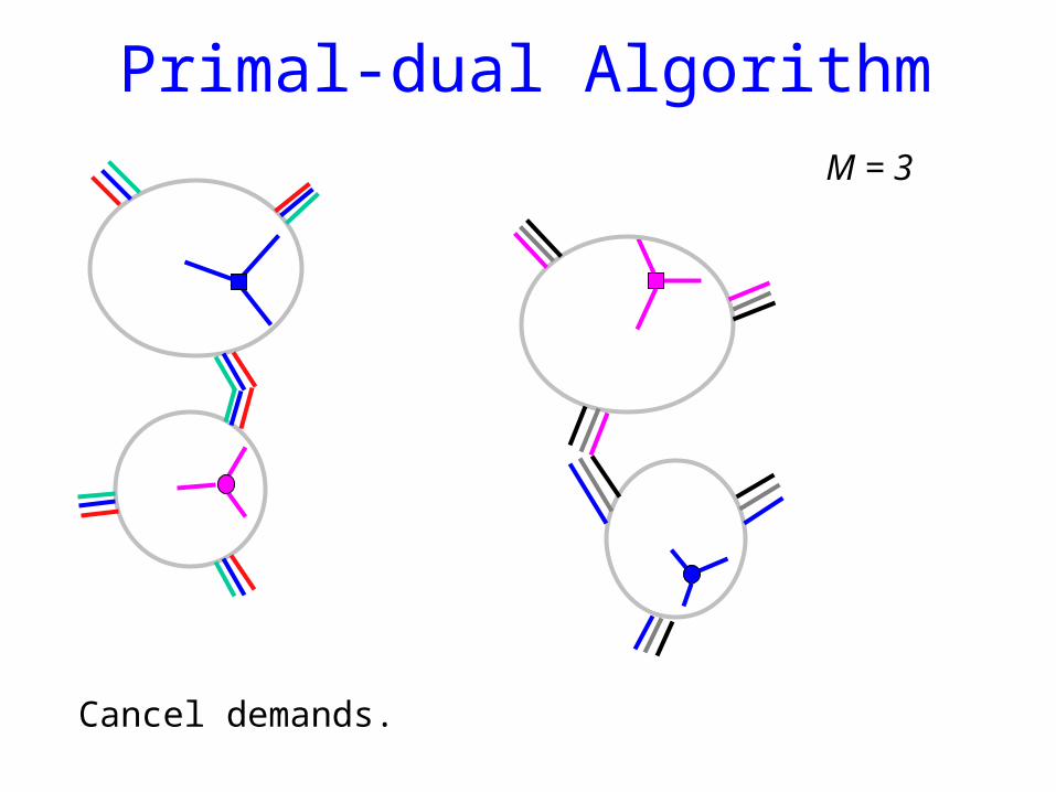
Primal-dual AlgorithmM = 3
Cancel demands.
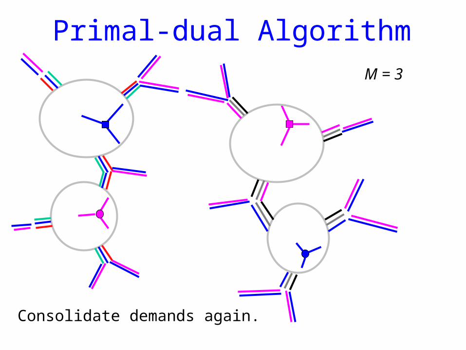
Primal-dual AlgorithmM = 3
Consolidate demands again.
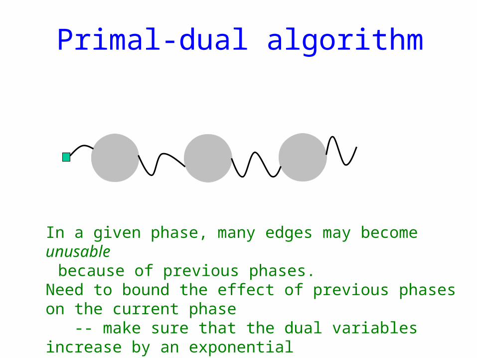
Primal-dual algorithm
In a given phase, many edges may become unusable because of previous phases. Need to bound the effect of previous phases on the current phase -- make sure that the dual variables increase by an exponential factor in successive phases.
Open Problems
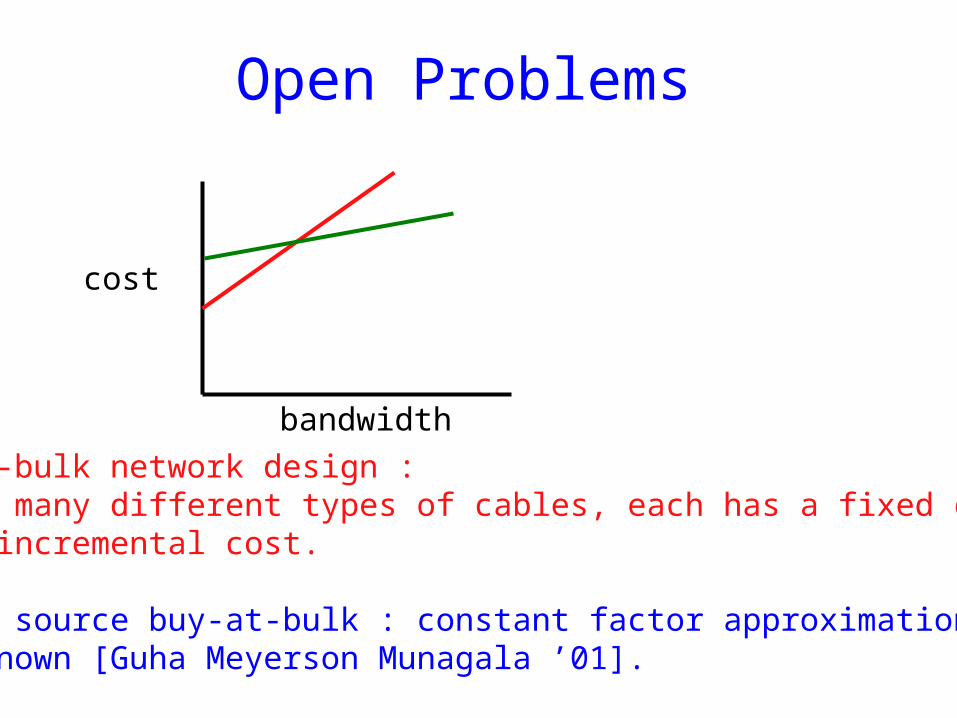
• buy-at-bulk network design : have many different types of cables, each has a fixed cost and an incremental cost. Single source buy-at-bulk : constant factor approximation algorithm known [Guha Meyerson Munagala ’01].
bandwidth
cost
Open Problems
• Buy-at-bulk : even for single cable nothing better than logarithmic factor known [Awerbuch Azar ’97].
• Single source rent-or-buy : what if different edges have different buying costs ? Nothing better than logarithmic factor known [Meyerson Munagala Plotkin ’00].