Embed Size (px)
Citation preview

Matthias Goltz
A CONTRIBUTION TO MONITORING OF EMBANKMENT
DAMS BY MEANS OF DISTRIBUTED FIBRE OPTIC
MEASUREMENTS


Die Dissertation repräsentiert die Ergebnisse des Forschungsprojektes „Verteilte
faseroptische Messungen zur Talsperrenüberwachung“, welches durch die TIWAG -
Tiroler Wasserkraft AG beauftragt und finanziert wurde. Des Weiteren wurden die
Ergebnisse des Forschungsprojektes „Optimierung von Aufheizkabeln zur verteilten
Filtergeschwindigkeitsmessung“, welches durch die Bayrische Forschungsstiftung
(BFS) und dem Unternehmenspartner LEONI Fibre Optics GmbH finanziert wurde in
der Arbeit berücksichtig.
Die vorliegende Dissertation wurde im August 2011 an der Leopold-Franzens-
Universität Innsbruck eingereicht.
Betreuer / Erstbegutachter
Univ.-Prof. Dr.-Ing. habil. Markus Aufleger
Arbeitsbereich Wasserbau
Leopold-Franzens-Universität Innsbruck
Zweitbegutachter:
Prof. Dr. Abdallah I. Husein Malkawi
Jordan University of Science and Technology


Acknowledgement
This doctoral thesis results mainly from the research projects “Monitoring of dams
using distributed fibre optic measurements” funded by the Tiroler Wasserkraft AG
(TIWAG) and “Optimization of heat-up cables for distributed filter velocity measure-
ments” funded by the Bayrischen Forschungsstiftung (BFS). I would like to thank the
TIWAG and the BFS for enabling the research through their financial support. I would
also like to extend my thanks to LEONI Fibre Optics GmbH, who also supported this
work.
I greatly thank my doctoral advisor Univ. Prof. Dr.-Ing. habil. Markus Aufleger for his
suggestions, guidance and support during my time at the Technische Universität
München and Universität Innsbruck. I also wish to thank my second supervisor Prof.
Dr. Abdallah I. Husein Malkawi for his input and constructive comments on this man-
uscript.
Also I would like to thank Ao.Univ.-Prof. Dipl.-Ing. Dr. Rudolf Stark for taking over the
chairmanship of the dissertation procedures.
I owe special thanks to Dipl. Geophys. Jürgen Dornstädter, Dr.-Ing. Peter Mucken-
thaler and Dr.-Ing. Sebastian Perzlmaier. Their support, ideas and advice significantly
contributed to the success of this work.
I also thank Orce Mangarovski from GD GRANIT a.d. Skopje and Stefan Hoppe from
Ofiteco who have supported the field work at the Knezovo Dam in Macedonia and
the Villalba Dam in Spain.
This work would have never been possible without the support from the staff of the
hydraulic laboratories both in Innsbruck and Obernach, and I would therefore like to
express my gratitude to them. I would also like to extend my thanks to all my col-
leagues in Innsbruck for their help and fruitful conversations with respect to the re-
search.
Last but not least special thanks are due to Evelyn and my parents for their support
and encouragement as well as Hanna Kiepas and Mathew Hoyes for reviewing this
work.
Finstersee, August 2011 Matthias Goltz

Abstract
Seepage through earth and hydraulic structures poses a substantial risk of damage
including dam breach due to internal erosion. Despite extensive research in the field
of internal erosion, the potential hazards resulting from internal erosion remain rela-
tively high. One of the reasons is that conventional monitoring systems can only
detect the time delayed processes of internal erosion when they are already far ad-
vanced.
The presented work is a contribution to the development of a monitoring system
which is based on distributed fibre optic measurements for holistic monitoring of
seepage and early detection of internal erosion in embankment dams and their foun-
dations. The proof of the applicability and general functioning of such a monitoring
system could be provided by the results of laboratory tests in which the fibre optic
cable was exposed to the expected loads. Furthermore, laboratory tests for leakage
detection and distributed filter velocity measurements were carried out with different
types of fibre optic cables and different soils to complement existing data. With re-
gard to the early detection of sink holes and low stress zones, the laboratory testing
program included experiments on distributed fibre strain sensing. Moreover, recent
installations of monitoring systems based on distributed fibre optic temperature
measurements in embankment dams are presented.
Kurzfassung
In den Strukturen des Grund- und Wasserbaus können überall dort, wo Erdstoffe
durchströmt werden, durch innere Erosion bedingte Schäden bis hin zu
Dammbrüchen auftreten. Trotz umfangreicher Forschungsarbeiten bleibt das aus der
inneren Erosion resultierende Gefährdungspotential nach wie vor relativ hoch. Das
liegt nicht zuletzt daran, dass die zeitlich verzögerten Vorgänge bei innerer Erosion
mit bisherigen Überwachungssystemen nur sehr spät erkennbar sind.
Die vorliegende Arbeit ist ein Beitrag zur Entwicklung eines Messsystems basierend
auf verteilten faseroptischen Messungen, welches die ganzheitliche Überwachung
der Durchströmung und die Früherkennung von Erosionsvorgängen im Innern von
Staudämmen und deren Gründung ermöglichen soll. Der Nachweis der Anwend-
barkeit und Funktionstüchtigkeit eines solchen Messsystems konnte durch Grundla-
genversuche, in denen die zur erwartenden Belastungen des Glasfaserkabels simu-
liert wurden, erbracht werden. Des Weiteren wurden zur Ergänzung bestehender
Datensätze, Versuche zur Leckageortung und verteilten Fil-
tergeschwindigkeitsmessung mit verschiedenen Kabeln und Böden durchgeführt. Im

Hinblick auf die frühzeitige Erkennung von Setzungstrichtern und Auflockerungszo-
nen beinhaltete das Versuchsprogramm zudem Grundlagenversuche zur verteilten
faseroptischen Dehnungsmessung. Zudem werden zwei Beispiele aus der Praxis
vorgestellt bei denen kürzlich Überwachungssysteme installiert wurden, welche auf
verteilten faseroptischen Temperaturmessungen beruhen.

Contents V
Contents
Acknowledgement I
Abstract III
Kurzfassung III
Contents V
Notation IX
1 Introduction 1
1.1 General 1
1.2 Objectives and scope of study 2
1.3 Layout and content 2
2 Literature review 5
2.1 Theoretical background 5
2.1.1 Characterization of porous media 5
2.1.2 Geometric models for the structure of porous media 10 2.1.2.1 General 10 2.1.2.2 Sphere packings 10
2.1.3 Flow and transport of particles in porous media 14 2.1.3.1 General 14 2.1.3.2 Reynolds number 16 2.1.3.3 Flow in porous media 16 2.1.3.4 Permeability of porous media 18 2.1.3.5 Pipe flow / Hagen-Poiseuille equation 21
2.1.4 Hydraulic criteria for particle transport in porous media 21 2.1.4.1 General 21 2.1.4.2 Particle settling velocity 22 2.1.4.3 Modified approach of Muckenthaler 26
2.2 Instrumentation of embankment dams 30
2.2.1 General 30
2.2.2 Monitoring concept 31
2.2.3 Loads and effects from the surrounding environment 33
2.2.4 Response parameters 34 2.2.4.1 Seepage 34 2.2.4.2 Pore pressure 35
VI Contents
2.2.4.3 Surface displacement 36 2.2.4.4 Displacement and deformation 36
2.2.5 Visual inspection 37
2.3 Internal erosion in embankment dams 38
2.3.1 General 38
2.3.2 Mechanism of failure 39
2.3.3 Time for development of internal erosion 45
2.3.4 Detectability of internal erosion 46
2.4 Geophysical methods for detection of internal erosion 47
2.4.1 General 47
2.4.2 Self-potential method 47
2.4.3 Resistivity method 48
2.4.4 Temperature measurements 49
2.4.5 Other methods 51
3 Distributed fibre optic measurements in embankment dams 53
3.1 General 53
3.2 Distributed fibre optic temperature measurements 53
3.2.1 Measuring system 53
3.3 Leakage detection and filter velocity measurements 56
3.3.1 General 56
3.3.2 Heating of the fibre optic cables 56
3.3.3 Theoretical background of distributed filter velocity measurement 57
3.3.4 Typical Applications 67
3.4 Distributed fibre optic strain measurements 69
3.4.1 General 69
3.4.2 Measuring principle 69
3.4.3 Applications 70
4 Laboratory tests 73
4.1 General 73
4.2 Laboratory tests for distributed filter velocity measurements 73
4.2.1 General 73
4.2.2 Laboratory tests on different soil materials 74 4.2.2.1 Description of tests 74 4.2.2.2 Performed tests 78

Contents VII
4.2.2.3 Discussion of results 83 4.2.3 Laboratory tests for optimized heat-up cables 86
4.2.3.1 Description of tests 86 4.2.3.2 Performed tests 87 4.2.3.3 Discussion of results 91
4.3 Laboratory tests to determine influence of mechanical stress 95
4.3.1 General 95
4.3.2 Laboratory test for investigation of influence of pressure
perpendicular to the cable axis 95 4.3.2.1 Description of tests 95 4.3.2.2 Performed tests 97 4.3.2.3 Discussion of the results 101
4.3.3 Laboratory test for investigation of influence of strain 111 4.3.3.1 Description of tests 111 4.3.3.2 Discussion of the results 112
4.4 Laboratory tests for distributed strain sensing 113
4.4.1 General 113
4.4.2 Description of tests 114
4.4.3 Performed tests 117
4.4.4 Analysis of the results 120
5 Recent application examples 127
5.1 General 127
5.2 Knezovo asphalt core rockfill dam 127
5.2.1 Situation 127
5.2.2 Layout 128
5.2.3 First measurements and leakage simulation tests 130
5.3 Villalba zoned earthfill dam 132
5.3.1 Situation 132
5.3.2 Layout 133
5.3.3 First measurements and leakage simulation tests 135
5.4 Remarks on the planning of leakage detection systems 139
5.4.1 Factors that can cause defects in the sealing elements 139
5.4.2 Frequency of measurements 139
5.5 Remarks on the determination of critical flow velocity 140
6 Summary and conclusions 147
6.1 Distributed fibre optic temperature sensing 147
VIII Contents
6.2 Distributed fibre optic temperature and strain sensing 149
Bibliography 151
Appendix A: Data sheets of investigated hybrid cables 161
Cable 1 161
Cable 2 163
Cable 3 164
Cable 4 166
Cable 5 168
Appendix B: Results of tests to determine influence of mechanical stress 171
Appendix C: Data sheets of investigated strain cables 179
Sensornet Damsense cableTM
179
Smartec SMARTprofile cable 180
Appendix D: Results of laboratory tests for distributed strain sensing 183

Notation IX
Notation1
Theoretical background (Chapter 2.1)
angle °
c ratio between dc and dz -
fl unit weight of the fluid kN/m3
fl dynamic viscosity of the fluid N∙s/m2
Kozeny – Carman constant -
friction factor -
fl kinematic viscosity m2/s
s density of the solid particles kg/m3
fl density of the fluid kg/m3
c Shields factor -
0 critical shear stress N/mm2
A area m2
Az pore area m2
B width m
cD drag coefficient -
Cc coefficient of curvature -
Cu coefficient of uniformity -
CH Hazen empirical coefficient -
e void ratio -
d10 10% fractile of particle size distribution m
d17 17% fractile of particle size distribution m
d30 30% fractile of particle size distribution m
d60 60% fractile of particle size distribution m
dc diameter of circle inscribing the gap, constriction size m
dp particle diameter m
1 To avoid duplication and thereby caused inconsistencies a topic related allocation of the sym-
bols is used.

X Notation
deff effective particle diameter m
d̄p,h effective hydraulic diameter of the pore channel m
dH hydraulic diameter m
dz diameter of the circle coextensive to the gap m
D pipe diameter m
g gravitational acceleration m/s2
Fres resisting force kN
H height m
i hydraulic gradient -
kf permeability m/s
ks roughness coefficient -
lv viscous length m
L projected length m
Le actual pore channel length m
n total porosity -
neff effective porosity -
Q flow rate m3/s
r radius m
Re Reynolds number -
Rep particle Reynolds number -
SF shape factor -
T tortuosity -
VG total of bulk volume of material m3
VH volume of pore water (retained water) m3
VP volume of void space m3
w velocity m/s
w̄ average velocity m/s
w* critical shear velocity m/s
wa average velocity in the pore system m/s
wc critical velocity m/s
wf filter velocity m/s
wp pore velocity m/s
wr relative velocity m/s

Notation XI
y distance in y-direction m
Distributed fibre optic measurements in embankment dams (Chapter 3)
angle °
c critical angle °
T heat transfer coefficient W/(m2∙K)
T thickness of thermal boundary layer m
vB Brillouin frequency shift Hz
difference in strain -
T difference in temperature K
porosity -
w porosity (considering wall effect) -
thermal conductivity W/(m∙K)
eff effective thermal conductivity W/(m∙K)
fl thermal conductivity of the fluid phase W/(m∙K)
s thermal conductivity of the solid phase W/(m∙K)
M thermal conductivity of cable jacket W/(m∙K)
fl kinematic viscosity m2/s
Kozeny – Carman constant -
thermal diffusivity m2/s
eff effective thermal diffusivity m2/s
density kg/m3
fl density of the fluid kg/m3
el specific electric resistance ∙mm2/m
A cross section m2
Ael conductor cross section m2
c specific heat capacity J/(kg∙K)
cp,fl specific heat capacity of the fluid phase J/(kg∙K)
cp,s specific heat capacity of the solid phase J/(kg∙K)
C strain coefficient of the optical fibre -

XII Notation
CT temperature coefficient of the optical fibre -
d diameter m
deff effective particle diameter m
dTc temperature difference between core and cable jacket K
dTint temperature increase due to heating K
dTsur temperature difference between cable jacket and surrounding material K
D diameter of the cylindrical heat source (cable) m
I current A
L length of conductor m
Nu Nusselt number -
Nueff effective Nusselt number -
Nucond apparent Nusselt number for heat conduction -
P rated power W
Preff effective Prantl number -
q heat flow J/s W
ql heat input per length W/m
r radius m
rext external radius m
rint internal radius m
Rep particle Reynolds number -
ReD Reynolds number of the cylinder -
Rel electric resistance
RT thermal resistance
S degree of saturation -
t time s
T temperature K
T0 initial temperature K
Tint internal temperature K
Tfl temperature of the fluid phase K
Tw temperature at the wall K
U voltage V
v0 frequency of light source Hz
vR Raman frequency shift Hz

Notation XIII
w velocity m/s
x characteristic overflow length m
Laboratory tests (Chapter 4)
porosity -
strain resolution
T temperature resolution K
eff,exp effective thermal conductivity (experimental determination) W/(m∙K)
s thermal conductivity of the solid phase W/(m∙K)
s,exp density of the solid (experimental determination) kg/m3
d,exp dry density (experimental determination) kg/m3
load kN/m2
max maximum load kN/m2
Cu coefficient of uniformity -
cp specific heat capacity J/(kg∙K)
d0 minimum particle size m
d100 maximum particle size m
d15 15% fractile of particle size distribution m
deff effective particle diameter m
deff effective particle diameter m
dmax maximum particle size m
D cable diameter m
kf,cal permeability (calculated) m/s
msp specific mass kg/m2
n porosity -
Recent application examples (Chapter 5)
Cu coefficient of uniformity -
dmax,e,cal calculated diameter of the largest erodible particle mm
dmax,e,test diameter of the largest erodible particle obtained from test mm

XIV Notation
dp particle size mm
kf permeability m/s
neff effective porosity -
ql heat input per length W/m
T tortuosity -
wcrit critical velocity m/s
wf,crit critical filter velocity m/s
w̄p average pore velocity m/s
ws particle settling velocity m/s
Chapter 1 1
1 Introduction
1.1 General
Internal erosion processes represent a substantial hazard potential for the integrity
and durability of hydraulic structures, especially of embankment dams and dykes.
Even after years of successful operation the hazard potential still remains relatively
high due to delayed processes which cannot be easily detected by current monitoring
systems. For new embankment dams, the likelihood of internal erosion failure can be
greatly reduced by proper design and provision of filters, which intercept seepage
through the embankment and the foundations to prevent continuing and progression
of internal erosion. However, even for well-designed dams with properly designed
filters there is always some risk for an erosion accident since the factors influencing
the initiation of erosion include zones of high permeability due to frost and thawing,
poor compaction, cracks due to seismic load, differential settlement or hydraulic
fracturing as well as many others.
A lot of research work concentrates on theoretical models to assess the risk of inter-
nal erosion in embankment dams or on laboratory tests to determine the filter and
erosion behaviour of soils. However, besides better risk assessment and better un-
derstanding of the filter and erosion behaviour of typically used soils, the early detec-
tion of internal erosion has to also be considered an important task. For embankment
dams water infiltrations should be closely monitored since each deviation from the
normal state may indicate processes of internal erosion. Generally, measurements of
the quantity of seepage water and pore pressure measurements give an indication of
the global seepage behaviour of an embankment dam. Additional possibilities for
more detailed survey of seepage conditions consist of geophysical methods, such as
resistivity measurements, self-potential measurements and or temperature meas-
urements. Temperature measurements are an indirect means to determine the pres-
ence and location of seepage flows in dams. They also allow an estimation of the
intensity of the seepage flow. Typically, thermocouples and thermistors have been
used for temperature measurements. In the 1980s distributed fibre optic temperature
measurements using optical fibres were developed, allowing the measurement of the
temperature distribution along a fibre optic cable. During recent years, this technique
has been constantly improved and nowadays offers very high accuracy in tempera-
ture measurement with the necessary spatial resolution. Since adequate methods for
internal erosion detection should consist of taking distributed measurements in real
time, distributed fibre optic measurements are well suited to accomplish this task.
Distributed fibre optic temperature measurements have been successfully used for
dam monitoring throughout the world during the last 15 years. However, so far the

2 Chapter 1
typical applications for embankment dams have been the monitoring of surface seal-
ings, mostly with focus of the perimetric joint. The presented work is a contribution to
the development of a monitoring system for holistic monitoring of seepage and early
detection of internal erosion in embankment dams with a central core and their foun-
dations.
1.2 Objectives and scope of study
The main objective of the presented work is the investigation of the suitability of dis-
tributed fibre optic measurements with respect to the development of a system for
holistic monitoring of seepage and early detection of internal erosion in embankment
dams and their foundations.
With regard to the main objective the following issues have been worked through:
Effects of mechanical loading of the fibre optic cable on the results of distributed fibre
optic temperature measurements.
Laboratory tests for filter velocity measurements and leakage detection with different
types of fibre optic cables and different soils to complement existing data.
Review of the approach to processing and analysing of data obtained by distributed
fibre optic temperature measurements.
Review and further development of existing approaches to assess the critical seep-
age velocity which causes transport of fine particles in embankment dams and their
foundation.
Determination of the measuring range, accuracy and repeatability of distributed fibre
optic strain sensing.
1.3 Layout and content
Chapter 2 contains the results of the literature review. In addition to the description of
the theoretical background for a better understanding of the geohydraulic processes,
an overview of instrumentation and monitoring of embankment dams are given. Fur-
thermore, this chapter is concerned with the internal erosion in zoned embankment
dams and presents the most common geophysical methods used for detection of
internal erosion and suffusion.
Chapter 3 introduces distributed fibre optic measurements. It delivers insight into the
measuring principle of distributed fibre optic temperature measurements and pro-
vides the theoretical background of distributed filter velocity measurements. Addition-
ally, examples for typical applications of distributed fibre optic temperature measure-

Chapter 1 3
ments for leakage detection are given. The chapter also presents the measuring
principle and possible applications of distributed fibre optic strain sensing.
In chapter 4, the laboratory tests, which were carried out, are presented. It includes
the experiments to prove the applicability and general functioning of distributed fibre
optic temperature measurements under conditions where the fibre optic cable is
exposed to strain and pressure perpendicular to the cable axis. Furthermore, it dis-
cusses the laboratory tests for leakage detection and distributed filter velocity meas-
urements as well as the experiments on distributed fibre strain sensing.
Chapter 5 presents insights regarding leakage detection in embankment dams with
central cores using two recent application examples. This chapter also gives remarks
on the planning of the leakage detection system and on the determination of the
critical flow velocity.
The findings of this thesis are concluded in chapter 6.

4 Chapter 1

Chapter 2 5
2 Literature review
2.1 Theoretical background
2.1.1 Characterization of porous media
Porous media can be described as a multiphase system consisting of a solid material
containing pores (solid phase) which are filled with liquid (liquid phase) or gas (gase-
ous phase). This multiphase system can be characterized by the parameters set out
in the following.
Porosity
One of the most important parameter is the porosity of a medium. It is given by:
G
P
V
Vn Eq. 2-1
and
G
HPeff
V
VVn
Eq. 2-2
With n total porosity
neff effective porosity
VP volume of void-space [m3]
VG total or bulk volume of material [m3]
VH volume of pore water (retained water) [m3]
The ratio of the volume of void-space to the bulk volume of material is described by
the void ratio e.
n
ne
1 Eq. 2-3
The total porosity n can be determined from the bulk density of the soil. However, for
ground water flow, as well as for the particle transport, the effective porosity neff is
more important. The effective porosity refers to the fraction of the total volume in
which fluid flow is effectively taking place. Fig. 2-1 shows the relationship between
the total porosity, effective porosity and the proportion of pore water as a function of
the particle size.
6 Chapter 2
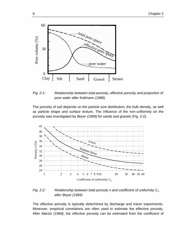
Fig. 2-1: Relationship between total porosity, effective porosity and proportion of
pore water after Kollmann (1986)
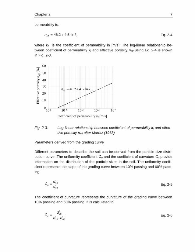
The porosity of soil depends on the particle size distribution, the bulk density, as well
as particle shape and surface texture. The influence of the non-uniformity on the
porosity was investigated by Beyer (1969) for sands and gravels (Fig. 2-2).
Fig. 2-2: Relationship between total porosity n and coefficient of uniformity Cu
after Beyer (1969)
The effective porosity is typically determined by discharge and tracer experiments.
Moreover, empirical correlations are often used to estimate the effective porosity.
After Marotz (1968), the effective porosity can be estimated from the coefficient of
Clay Silt
Po
re v
olu
me
[%]
Gravel Stones
0
30
60
pore water
Sand
24
26
28
30
32
34
36
38
40
42
1 10
loose
medium dense
dense
42
38
36
34
32
30
28
26
24
40
1 2 3 4 5 6 7 8 910 20 30 40 50 60
Coefficient of uniformity Cu
Poro
sity
n [
%]
Chapter 2 7
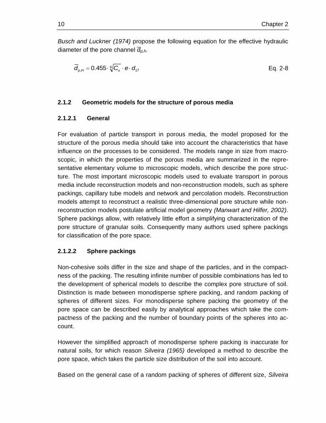
permeability to:
feff kn ln5.42.46 Eq. 2-4
where kf is the coefficient of permeability in [m/s]. The log-linear relationship be-
tween coefficient of permeability kf and effective porosity neff using Eq. 2-4 is shown
in Fig. 2-3.
Fig. 2-3: Log-linear relationship between coefficient of permeability kf and effec-
tive porosity neff after Marotz (1968)
Parameters derived from the grading curve
Different parameters to describe the soil can be derived from the particle size distri-
bution curve. The uniformity coefficient Cu and the coefficient of curvature Cc provide
information on the distribution of the particle sizes in the soil. The uniformity coeffi-
cient represents the slope of the grading curve between 10% passing and 60% pass-
ing.
10
60
d
dCu Eq. 2-5
The coefficient of curvature represents the curvature of the grading curve between
10% passing and 60% passing. It is calculated to:
6010
2
30
dd
dCc
Eq. 2-6
0.00
10.00
20.00
30.00
40.00
50.00
60.00
1.00E-05 1.00E-04 1.00E-03 1.00E-02 1.00E-01
Coefficient of permeability kf [m/s]
10-110-310-410-5
Eff
ecti
ve
poro
sity
nef
f[%
]
0
10
20
30
40
50
60
10-2
feff kn ln5.42.46

8 Chapter 2
Depending on the shape of the particle size distribution curve, soils are classified as
either well graded or poorly graded. For poorly graded soils it is further differentiated
between uniformly graded soil and gap graded soils. Well graded soils contain a wide
range of particle sizes and give good representation of all the sizes they contain.
Additionally the shape of the particle size distribution curve is to be smooth. Accord-
ing to the unified soil classification system (USCS) well graded gravels must have a
Cu value greater than 4 and well graded sands must have a Cu value greater than 6.
Additionally for well graded sands and gravel, the Cc value has to lie between 1 and
3. In contrast to the well graded soil, a uniformly graded soil is a soil that contains
particles of mostly one size. A gap graded soil, is a soil that consists of both large
and small particles, but at least one particle size in between is absent.
The uniformity coefficient and the coefficient of curvature can be used as indicators
for engineering properties of granular soils such as compressibility and hydraulic
conductivity.
Particle shape
The particle shape and surface texture of the grains also have an influence on the
pore structure and thus on the porosity of the granular soils. The more the particle
shape differs from spherical shape, the greater is the porosity. Kozeny (1927) there-
fore introduces a particle shape factor (see Fig. 2-4 and Tab. 2-1), which is used in
different empirical equations as a correction factor.
Fig. 2-4: Particle shapes according to Busch and Luckner (1974)

Chapter 2 9
Tab. 2-1: Shape factor for soil particles according to Busch and Luckner (1974)
Particle shape Shape factor SF
a) Spherical 1.0
b) Platy 1.1
c) Spicular 1.2
d) Round 1.0 – 1.1
e) Edged 1.2
f) Sharp-edged 1.3
Pore space geometry
The described parameters have a decisive influence on the pore space geometry.
Because of the complexity of the pore space geometry, even for simple sphere pack-
ings, simplified parameters to describe the geometry are usually resorted to. The
most important parameters are the effective particle diameter deff and the effective
hydraulic diameter of the pore channel d̄p,h. These parameters are derived from the
grading curve and are used to evaluate particle transport in porous media.
The effective particle diameter of granular soils can be calculated from the grading
curve using the arithmetic, geometric (log linear) or harmonic mean of all fractions.
Usually the harmonic mean of all fractions is used, since it is related to the specific
surface of the grains. Accordingly, deff can be calculated to:
1
1
,
n
i i
im
effd
qd Eq. 2-7
with i Index of the fraction with the limits du and dl
qm,i ith fraction of particle between limits du and dl
di harmonic mean of ith fraction 2∙du·dl/(du+dl)
n number of fractions
10 Chapter 2
Busch and Luckner (1974) propose the following equation for the effective hydraulic
diameter of the pore channel d̄p,h.
176
, 455.0 deCd uHp Eq. 2-8
2.1.2 Geometric models for the structure of porous media
2.1.2.1 General
For evaluation of particle transport in porous media, the model proposed for the
structure of the porous media should take into account the characteristics that have
influence on the processes to be considered. The models range in size from macro-
scopic, in which the properties of the porous media are summarized in the repre-
sentative elementary volume to microscopic models, which describe the pore struc-
ture. The most important microscopic models used to evaluate transport in porous
media include reconstruction models and non-reconstruction models, such as sphere
packings, capillary tube models and network and percolation models. Reconstruction
models attempt to reconstruct a realistic three-dimensional pore structure while non-
reconstruction models postulate artificial model geometry (Manwart and Hilfer, 2002).
Sphere packings allow, with relatively little effort a simplifying characterization of the
pore structure of granular soils. Consequently many authors used sphere packings
for classification of the pore space.
2.1.2.2 Sphere packings
Non-cohesive soils differ in the size and shape of the particles, and in the compact-
ness of the packing. The resulting infinite number of possible combinations has led to
the development of spherical models to describe the complex pore structure of soil.
Distinction is made between monodisperse sphere packing, and random packing of
spheres of different sizes. For monodisperse sphere packing the geometry of the
pore space can be described easily by analytical approaches which take the com-
pactness of the packing and the number of boundary points of the spheres into ac-
count.
However the simplified approach of monodisperse sphere packing is inaccurate for
natural soils, for which reason Silveira (1965) developed a method to describe the
pore space, which takes the particle size distribution of the soil into account.
Based on the general case of a random packing of spheres of different size, Silveira
Chapter 2 11
(1965, 1975) developed approaches to calculate the pore constriction size distribu-
tion for the densest state and the loosest state. Muckenthaler (1989) and Schuler
(1997) improved the method and facilitated the implementation. More recently,
among others Locke (2001), Indraratna (2007) and Reboul (2008) dealt with sphere
packings for the description of granular soils.
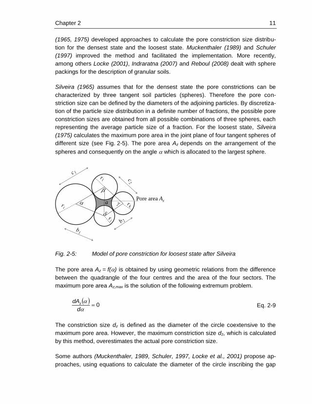
Silveira (1965) assumes that for the densest state the pore constrictions can be
characterized by three tangent soil particles (spheres). Therefore the pore con-
striction size can be defined by the diameters of the adjoining particles. By discretiza-
tion of the particle size distribution in a definite number of fractions, the possible pore
constriction sizes are obtained from all possible combinations of three spheres, each
representing the average particle size of a fraction. For the loosest state, Silveira
(1975) calculates the maximum pore area in the joint plane of four tangent spheres of
different size (see Fig. 2-5). The pore area Az depends on the arrangement of the
spheres and consequently on the angle which is allocated to the largest sphere.
Fig. 2-5: Model of pore constriction for loosest state after Silveira
The pore area Az = f() is obtained by using geometric relations from the difference
between the quadrangle of the four centres and the area of the four sectors. The
maximum pore area Az,max is the solution of the following extremum problem.
0
d
dAz Eq. 2-9
The constriction size dz is defined as the diameter of the circle coextensive to the
maximum pore area. However, the maximum constriction size dz, which is calculated
by this method, overestimates the actual pore constriction size.
Some authors (Muckenthaler, 1989, Schuler, 1997, Locke et al., 2001) propose ap-
proaches, using equations to calculate the diameter of the circle inscribing the gap
aPore area Az

12 Chapter 2
between the particles exactly. However, the computational effort increases exponen-
tially with the number of particle diameters representing the different fractions, due to
the increasing number of possible combinations. Moreover, the proposed approaches
are not universally applicable.
However, there is also broad agreement, that the distribution of the pore constriction
sizes for the densest state and the loose state are almost parallel to the exact distri-
bution of pore constriction sizes (Muckenthaler, 1989, Wittmann, 1980). The ratio c
between the diameter of the circle inscribing the gap dC, and the diameter of the
circle coextensive to the gap dz can be easily calculated for monodisperse sphere
packings (Fig. 2-6).
Fig. 2-6: Pore area Az and Aincircle for monodisperse sphere packing
The diameter of the circle coextensive to the gap dz is calculated using the following
equations:
4
42
22
z
z
drrA Eq. 2-10
42 rd z
Eq. 2-11
The diameter of the circle inscribing the gap dc is calculated to
122 rdc . Eq. 2-12
Consequently, for the case of pore space between particles of equal size, the ratio c
is:
2r
2r
r 2r
2r
rPore Area Az
AIncircle

Chapter 2 13
79.0
4
12
z
cc
d
d
Eq. 2-13
This configuration is obtained for each particle diameter with the corresponding prob-
ability. For n fractions, there are as many nodes of the pore constriction size distribu-
tion, for which the exact solution of the diameter of the inscribed circle is obtained by
multiplying the approximate solution after Silveira with the ratio c. Therefore it is
assumed that it is feasible to obtain the more accurate distribution of constriction
sizes by calculating the diameter of the circle coextensive to the gap dz according to
Silveira and multiplying it with the ratio c for each possible constellation (Etzer,
2010). Taking into account, that both the idealization of soil particles by spheres and
the specification that the centres of all four spheres are within the same plane do not
correspond to reality, an exaggerated accuracy for determination of the constriction
size is not considered to be appropriate.
The probability of the occurrence of certain pore constriction sizes is determined
using the probability of the occurrence of the different fractions of particle size. In this
approach the particle size distribution by number as suggested by Ziems (1968) for
calculating the probability of occurrence of the pore constriction sizes is used. By this
means, a spectrum of pore constriction sizes with associated probability of occur-
rence is obtained from a discretized particle distribution curve which allows the illus-
tration of the pore constriction size distribution (CSD).
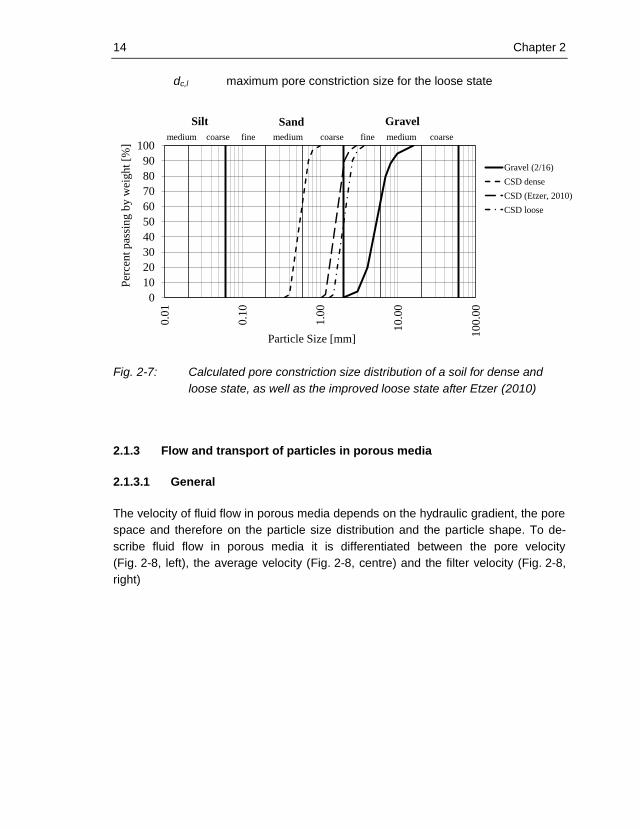
Fig. 2-7 shows the particle size distribution of a gravel together with the correspond-
ing constriction size distribution for the dense state and the loose state, as well as
tweaked constriction size distribution for the loose state after Etzer (2010).
The constriction size distribution for the dense state and the loose state form an
interval, which limits the actual constriction size distribution. Sensitivity analyses have
shown that the constriction size distribution for a given porosity can be interpolated
from the constriction size distribution of the densest state and the loose state at the
respective cumulative frequencies by the following equation:
where dc,d pore constriction size for the dense state
n porosity
dc,n maximum pore constriction size for the given porosity
dcdclcnc dddn
d ,,,,2169.0
2595.0
Eq. 2-14
14 Chapter 2
dc,l maximum pore constriction size for the loose state
Fig. 2-7: Calculated pore constriction size distribution of a soil for dense and
loose state, as well as the improved loose state after Etzer (2010)
2.1.3 Flow and transport of particles in porous media
2.1.3.1 General
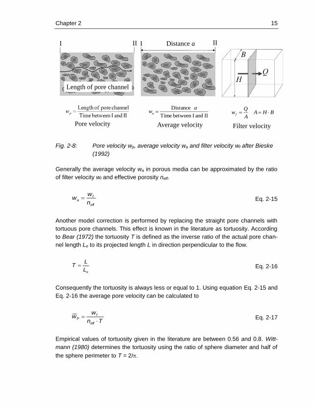
The velocity of fluid flow in porous media depends on the hydraulic gradient, the pore
space and therefore on the particle size distribution and the particle shape. To de-
scribe fluid flow in porous media it is differentiated between the pore velocity
(Fig. 2-8, left), the average velocity (Fig. 2-8, centre) and the filter velocity (Fig. 2-8,
right)
0
10
20
30
40
50
60
70
80
90
100
0.0
1
0.1
0
1.0
0
10
.00
10
0.0
0
Per
cen
t p
assi
ng
by
wei
gh
t [%
]
Particle Size [mm]
Gravel (2/16)
CSD dense
CSD (Etzer, 2010)
CSD loose
Silt Sand Gravel
fine medium coarsefine medium coarsemedium coarse
Chapter 2 15
Fig. 2-8: Pore velocity wp, average velocity wa and filter velocity wf after Bieske
(1992)
Generally the average velocity wa in porous media can be approximated by the ratio
of filter velocity wf and effective porosity neff.
eff
fa
n
ww
Eq. 2-15
Another model correction is performed by replacing the straight pore channels with
tortuous pore channels. This effect is known in the literature as tortuosity. According
to Bear (1972) the tortuosity T is defined as the inverse ratio of the actual pore chan-
nel length Le to its projected length L in direction perpendicular to the flow.
eL
LT Eq. 2-16
Consequently the tortuosity is always less or equal to 1. Using equation Eq. 2-15 and
Eq. 2-16 the average pore velocity can be calculated to
Tn
ww
eff
fP
Eq. 2-17
Empirical values of tortuosity given in the literature are between 0.56 and 0.8. Witt-
mann (1980) determines the tortuosity using the ratio of sphere diameter and half of
the sphere perimeter to T = 2/.
Length of pore channel
Distance aI II III
Pore velocity Average velocity Filter velocity
BHAA
Qw f
II and Ibetween Time
Distance awa
16 Chapter 2
2.1.3.2 Reynolds number
The Reynolds number Re as the ratio of inertial forces to viscous forces quantifies
the relative importance of these two types of forces for given flow conditions and is
therefore used to evaluate the flow regime. High Reynolds numbers indicate turbulent
flow while small Reynolds numbers indicate laminar conditions. For flow in a pipe or
tube, the Reynolds number is generally defined as:
fl
Hdw
Re Eq. 2-18
where w fluid velocity [m/s]
dH hydraulic diameter of the pipe [m]
fl kinematic viscosity [m2/s]
To characterize the flow nature in porous media the most common definition of the
Reynolds number is given by the following equation:
e
dw
fl
efffp
1Re
Eq. 2-19
where deff is effective particle diameter [m], fl the kinematic viscosity [m2/s], wf the
filter velocity [m/s] and e the void ratio.
2.1.3.3 Flow in porous media
Flow in porous media is characterized by the influence of inertial forces and viscous
forces. According to Trussell and Chang (1999) it can be distinguished between four
flow regimes which are shown in Fig. 2-9 and described in the following.
In the first regime (Darcy regime) the flow is laminar and influenced only by frictional
forces. Flow in this region is also named Darcy flow or creeping flow. It is limited to
Reynolds numbers ReP approximately below 1. With introduction of the proportionali-
ty factor kf (permeability), the linear relationship between the hydraulic gradient i and
the filter velocity wf is described by the Darcy law, which can be written as:
ikw ff Eq. 2-20
In the second flow regime (Forchheimer regime), which is described by particle

Chapter 2 17
Reynolds numbers ReP from 1 to about 100, flow is still strictly laminar. However,
with increasing flow the contribution of inertial forces increases. Thus the linear rela-
tionship between the hydraulic gradient and the filter velocity is no longer present.
According to Forchheimer (1930) the relationship between hydraulic gradient and
filter velocity can be described by the following quadratic equation:
2
ff wbwai Eq. 2-21
where a and b are constants. At the upper end of the Forchheimer regime the bulk of
head loss is significantly related on wf2. Also at the upper end stationary vortices are
formed in the cells between the grains.
The third regime represents the transition from more or less full inertial flow to full
statistical turbulence. The upper limit of this region is not well established, but is likely
to correspond to Reynolds numbers between 600 and 800, depending on the porous
media and flow conditions. The Forchheimer equation (Eq. 2-21) remains valid but
with another set of constants a and b (Burcharth and Andersen, 1995). At the lower
end of the flow regime, turbulence is just beginning to appear in some of the cells,
while at the upper end, turbulence is present in the bulk of those cells. Throughout
most of the flow regime vortices are regularly shed downstream of individual media
grains.
In the fourth flow regime, with correspondingly larger particle Reynolds numbers
turbulent flow is formed in the entire medium. Also for the turbulent regime the
Forchheimer equation (Eq. 2-21) approximates the relationship between the hydraulic
gradient and the filter velocity.

18 Chapter 2
Fig. 2-9: Flow regimes in porous media after Trussell and Chang (1999)
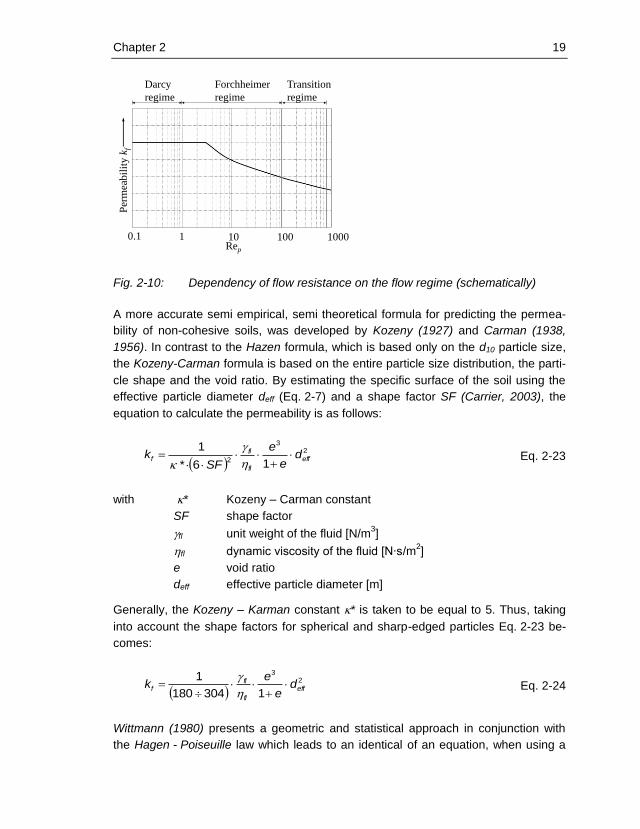
2.1.3.4 Permeability of porous media
The permeability coefficient kf representing the flow resistance of porous media is a
constant only for the laminar undisturbed flow (Fig. 2-10). With increasing influence of
inertial forces, vortices are formed in the cells between the grains, which lead to a
change in flow resistance. In general the permeability of soil is measured in the la-
boratory using conventional permeability tests. Besides that, there are empirical
methods for obtaining the permeability of a soil from measureable characteristics of
the soil such as particle size distribution and porosity of the media. One of the best-
known empirical formulas for determining the permeability of saturated sands is the
formula proposed by Hazen (1911, 1892):
2
10dCk Hf Eq. 2-22
Where kf [cm/s] is the permeability, CH the Hazen empirical coefficient and d10 [cm]
the particle size for which 10% of the soil is finer.
The empirical coefficient CH is taken to be 100. The formula’s applicability is general-
ly limited to narrow graded sands with Cu < 2 and 0.01 cm < d10 < 0.3 cm.
Creeping flow,
no inertial
influence
Darcy regime
Laminar flow,
increasing inertial
influence
Forchheimer regime Transition regime
Flow entirely
random
and irregular
Turbulent regime
Inertial flow with
increasing random,
irregular flow
ReK ~ 1 ReK ~ 100 ReK ~ 800
2
ff wbwai 2
ff wbwai f
f
k
wi
Chapter 2 19
Fig. 2-10: Dependency of flow resistance on the flow regime (schematically)
A more accurate semi empirical, semi theoretical formula for predicting the permea-
bility of non-cohesive soils, was developed by Kozeny (1927) and Carman (1938,
1956). In contrast to the Hazen formula, which is based only on the d10 particle size,
the Kozeny-Carman formula is based on the entire particle size distribution, the parti-
cle shape and the void ratio. By estimating the specific surface of the soil using the
effective particle diameter deff (Eq. 2-7) and a shape factor SF (Carrier, 2003), the
equation to calculate the permeability is as follows:
23
2 16*
1eff
fl
flf d
e
e
SFk
Eq. 2-23
with * Kozeny – Carman constant
SF shape factor
fl unit weight of the fluid [N/m3]
fl dynamic viscosity of the fluid [N∙s/m2]
e void ratio
deff effective particle diameter [m]
Generally, the Kozeny – Karman constant * is taken to be equal to 5. Thus, taking
into account the shape factors for spherical and sharp-edged particles Eq. 2-23 be-
comes:
2
3
1304180
1eff
fl
flf d
e
ek
Eq. 2-24
Wittmann (1980) presents a geometric and statistical approach in conjunction with
the Hagen - Poiseuille law which leads to an identical of an equation, when using a
Darcy
regime
Forchheimer
regime
Transition
regime
Rep
Per
mea
bil
ity
k f
1 100.1 100 1000

20 Chapter 2
coefficient of 1/180. According to Wittmann, the coefficient ranges from 1/270 to
1/180.
Eq. 2-22 and Eq. 2-23 are limited to laminar flow. In flow regimes, for which inertial
actions dominate, the flow resistance of the porous media can be described by using
the non-linear Forchheimer equation (Eq. 2-21). The coefficient a [s/m] of the linear
term in Eq. 2-21 depends on the properties of both the fluid and the porous medium.
It describes energy loss due to friction. The coefficient b [s2/m
2] depends solely on
the properties of the porous medium, such as porosity as well as size and shape of
the particles. It represents the influence of inertia forces on the flow resistance.
For many practical applications, it is not possible or too costly to determine the coeffi-
cient a and b in tests, therefore empirical relations have to be used. Sidiropoulou et
al. (2006) examined the empirical approaches of different researchers to determine
the coefficients a and b, and compared them with the experimental data available in
the literature. Based on their studies they recommend the calculation of the coeffi-
cients a and b according to the approach of Kadlec and Knight (1996), since this
approach provides the best agreement with published experimental results. Accord-
ingly the Forchheimer coefficients are calculated to:
27.3
)1(255
eff
fl
dng
na
Eq. 2-25
effdng
nb
3
)1(2
Eq. 2-26
where fl [m2/s] is the kinematic viscosity.
To take into account the dependence of the Forchheimer coefficients on the flow
regime characterised by ReP the following equations derived from the approach of
Hill and Koch (2002) can be used.
For 10 < ReP ≤ 80:
2
)1(6570
eff
fl
dg
na
Eq. 2-27
effdg
nb
)1(1.98
Eq. 2-28
and for ReP > 80:

Chapter 2 21
2
)1(6570
eff
fl
dg
na
Eq. 2-29
effdg
nb
)1(65.88
Eq. 2-30
2.1.3.5 Pipe flow / Hagen-Poiseuille equation
By substituting the porous media with a number of parallel circular capillaries, the
Hagen-Poiseuille law can be used for the simulation of flow through the media. As
mentioned in section 2.1.3.4, part of the approaches to estimate the permeability of
granular soil is based on this equation. The equation gives the pressure drop in a
fluid flowing through a long cylindrical pipe and takes the following form:
fl
iDgQ
128
4
Eq. 2-31
with Q flow rate [m3/s]
D pipe diameter [m]
i hydraulic gradient
fl kinematic viscosity of the fluid [m2/s] (water = 1.3·10
-6 m
2/s
for T = 10°C)
A special case of flow through porous media is the flow in tubular shaped defects.
2.1.4 Hydraulic criteria for particle transport in porous media
2.1.4.1 General
With the assumption that transport of fine particles through the pore structure is geo-
metrically possible, stability considerations using hydraulic parameters are required
to ascertain that particle transport does not occur. Most of the existing hydraulic crite-
ria are based completely or partially on laboratory tests using specific soil samples
and do not allow a conclusion to be drawn about the physical processes in the pore
structure. The extraction of particles from the grain structure and their further
transport in a through-flowed soil are essential processes in the erosion process.
Depending on the particle size and the boundary conditions, the particles are re-
leased both by colloidal forces and by hydrodynamic forces. In embankment dams,

22 Chapter 2
due to the used soil materials and the seepage velocities, hydrodynamic forces are
usually responsible for the release of particles. According to Zanke (1982), adhesion
forces, which might have to be overcome to release the fine particles, can be consid-
ered by the simplified assumption of an apparent increase in the specific weight. The
corresponding increase in the specific weight is calculated to:
2
6
,
109
p
sAsd
Eq. 2-32
with in [kg/m3] and dp in [m].
2.1.4.2 Particle settling velocity
According to Stokes, the settling velocity w of spherical particles with the density s
and the diameter dp in a fluid with the density fl and the dynamic viscosity can be
derived as:
fl
pdgw
2
18
1 Eq. 2-33
Where = (s - fl)/fl and g is gravitational acceleration.
By using the drag coefficient cD, the drag force of a sphere due to relative movement
in a fluid with the velocity wr is described as:
8
22 rflpDres
wdcF
Eq. 2-34
By equating the effective weight force to the expression of the drag force, i.e.
0668
3322
g
dg
dwdc fl
p
s
pflpD
Eq. 2-35
the drag coefficient cD can be expressed as:
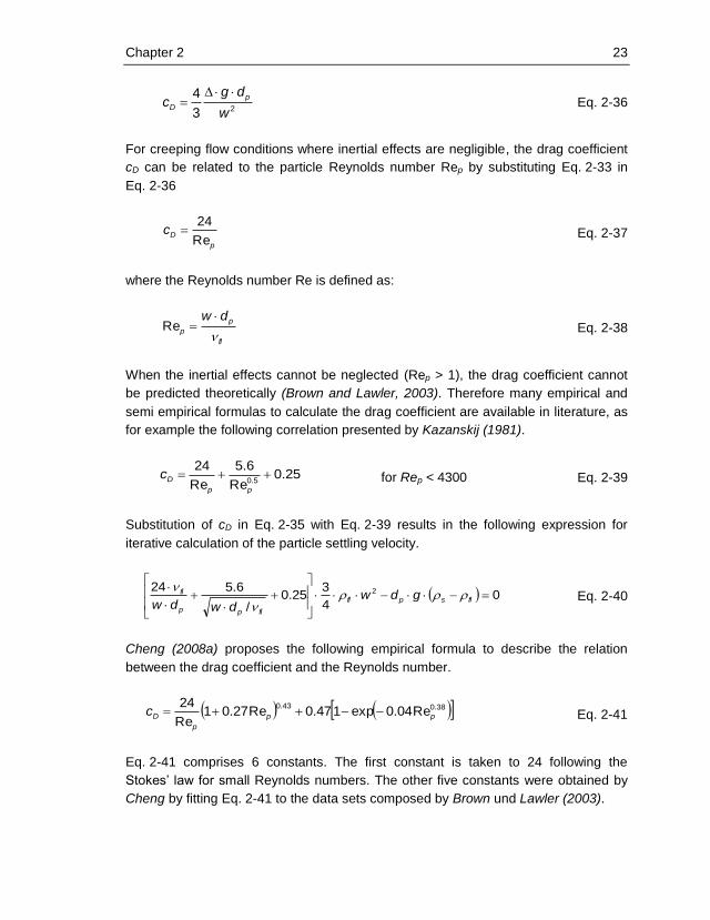
Chapter 2 23
23
4
w
dgc
p
D
Eq. 2-36
For creeping flow conditions where inertial effects are negligible, the drag coefficient
cD can be related to the particle Reynolds number Rep by substituting Eq. 2-33 in
Eq. 2-36
p
DcRe
24 Eq. 2-37
where the Reynolds number Re is defined as:
fl
p
p
dw
Re Eq. 2-38
When the inertial effects cannot be neglected (Rep > 1), the drag coefficient cannot
be predicted theoretically (Brown and Lawler, 2003). Therefore many empirical and
semi empirical formulas to calculate the drag coefficient are available in literature, as
for example the following correlation presented by Kazanskij (1981).
25.0Re
6.5
Re
245.0
pp
Dc for Rep < 4300 Eq. 2-39
Substitution of cD in Eq. 2-35 with Eq. 2-39 results in the following expression for
iterative calculation of the particle settling velocity.
04
325.0
/
6.524 2
flspfl
flpp
fl gdwdwdw
Eq. 2-40
Cheng (2008a) proposes the following empirical formula to describe the relation
between the drag coefficient and the Reynolds number.
38.043.0Re04.0exp147.0Re27.01
Re
24pp
p
Dc Eq. 2-41
Eq. 2-41 comprises 6 constants. The first constant is taken to 24 following the
Stokes’ law for small Reynolds numbers. The other five constants were obtained by
Cheng by fitting Eq. 2-41 to the data sets composed by Brown und Lawler (2003).
24 Chapter 2
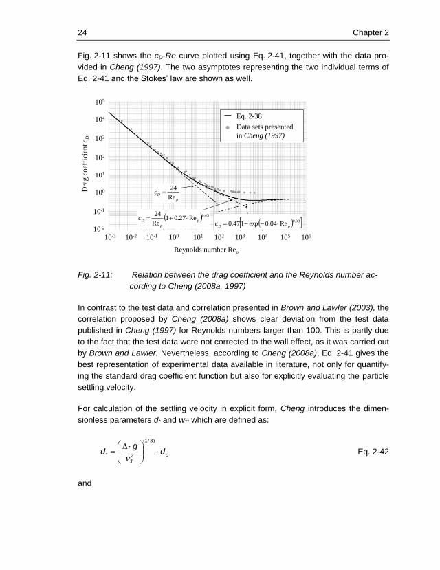
Fig. 2-11 shows the cD-Re curve plotted using Eq. 2-41, together with the data pro-
vided in Cheng (1997). The two asymptotes representing the two individual terms of
Eq. 2-41 and the Stokes’ law are shown as well.
Fig. 2-11: Relation between the drag coefficient and the Reynolds number ac-
cording to Cheng (2008a, 1997)
In contrast to the test data and correlation presented in Brown and Lawler (2003), the
correlation proposed by Cheng (2008a) shows clear deviation from the test data
published in Cheng (1997) for Reynolds numbers larger than 100. This is partly due
to the fact that the test data were not corrected to the wall effect, as it was carried out
by Brown and Lawler. Nevertheless, according to Cheng (2008a), Eq. 2-41 gives the
best representation of experimental data available in literature, not only for quantify-
ing the standard drag coefficient function but also for explicitly evaluating the particle
settling velocity.
For calculation of the settling velocity in explicit form, Cheng introduces the dimen-
sionless parameters d* and w** which are defined as:
p
fl
dg
d
)3/1(
2*
Eq. 2-42
and
10-3 10-2 10-1 100 101 102 103 104 105 106
10-2
10-1
100
101
102
103
104
105
Reynolds number Rep
Dra
g c
oef
fici
ent
c D
Eq. 2-38
Data sets presented
in Cheng (1997)
43.0Re27.01
Re
24p
p
Dc
p
DcRe
24
38.0Re04.0exp147.0 pDc

Chapter 2 25
wgw fl )3/1(
** Eq. 2-43
Thus, the flow resistance can be expressed as a function of d* similar to the depend-
ence of the flow resistance on the Reynolds number. Again, Cheng obtains the fol-
lowing correlation for cD by minimizing the deviation from the data compiled in Brown
and Lawler (2003).
45.0
*
54.03
*2
*
15.0exp147.0022.01432
ddd
cD Eq. 2-44
The dimensionless parameter w** is calculated by substituting Eq. 2-44 into the fol-
lowing equation:
Dc
dw
3
4 *** Eq. 2-45
Thus, by using the Eq. 2-42 to Eq. 2-45 the terminal settling velocity of spherical
particles can be expressed explicitly as a function of the particle diameter. Fig. 2-12
illustrates the corresponding settling velocity against the particle diameter as well as
the iteratively calculated settling velocity using Eq. 2-40 and the Stoke’s law. An
inspection of Fig. 2-12 demonstrates that the approach of Kazanskij (1981) and the
approach of Cheng (2008a) produce almost identical results.
Fig. 2-12: Settling velocity w in water (T = 20°C) for spherical particles (s =
2.6 g/cm3) depending on particle size dp
Particle size dp [mm]
10-3 10-2 10-1 100 101
10-5
10-4
10-3
10-2
10-1
100
Set
tlin
g v
elo
city
w[m
/s]
1.00E-03
1.00E-02
1.00E-01
1.00E+00
1.00E+01
1.00E+02
1.00E-03 1.00E-02 1.00E-01 1.00E+00 1.00E+01
Sin
kg
es
ch
win
dig
ke
it w
[c
m/s
]
Korndurchmesser dK [mm]
Sinkgeschwindigkeit
Stokes
Kazanskij (1981)
Cheng (2008)
26 Chapter 2
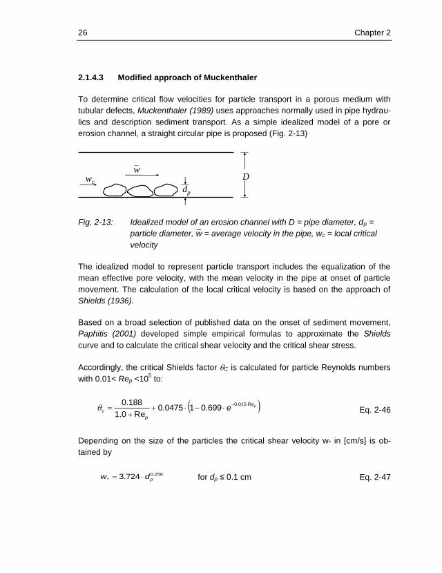
2.1.4.3 Modified approach of Muckenthaler
To determine critical flow velocities for particle transport in a porous medium with
tubular defects, Muckenthaler (1989) uses approaches normally used in pipe hydrau-
lics and description sediment transport. As a simple idealized model of a pore or
erosion channel, a straight circular pipe is proposed (Fig. 2-13)
Fig. 2-13: Idealized model of an erosion channel with D = pipe diameter, dp =
particle diameter, w̄ = average velocity in the pipe, wc = local critical
velocity
The idealized model to represent particle transport includes the equalization of the
mean effective pore velocity, with the mean velocity in the pipe at onset of particle
movement. The calculation of the local critical velocity is based on the approach of
Shields (1936).
Based on a broad selection of published data on the onset of sediment movement,
Paphitis (2001) developed simple empirical formulas to approximate the Shields
curve and to calculate the critical shear velocity and the critical shear stress.
Accordingly, the critical Shields factor C is calculated for particle Reynolds numbers
with 0.01< Rep <105 to:
pep
c
Re015.0699.010475.0
Re0.1
188.0
Eq. 2-46
Depending on the size of the particles the critical shear velocity w* in [cm/s] is ob-
tained by
256.0
* 724.3 pdw for dp ≤ 0.1 cm Eq. 2-47
wwc
dp
D

Chapter 2 27
569.0
* 656.7 pdw
for dp > 0.1 cm Eq. 2-48
and the critical shear stress 0 in [N/cm2] is calculated to
512.0
0 804.13 pd for dp ≤ 0.1 cm Eq. 2-49
569.0
0 479.58 pd
for dp > 0.1 cm Eq. 2-50
The approach of Muckenthaler (1989) for calculation of the critical velocity wc at on-
set of particle movement is based on the log law solution for the velocity distribution
in pipes. Tab. 2-2 summarizes the relevant equations to calculate the velocity distri-
bution.
The velocity distribution for turbulent pipe flow is calculated depending on the viscous
length l, which is defined as:
*w
l fl Eq. 2-51
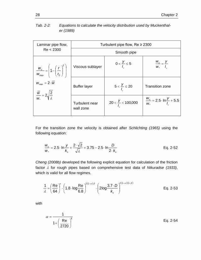
28 Chapter 2
Tab. 2-2: Equations to calculate the velocity distribution used by Muckenthal-
er (1989)
For the transition zone the velocity is obtained after Schlichting (1965) using the
following equation:
ss
c
k
D
k
y
w
w
2ln5.275.3
22ln5.2
* Eq. 2-52
Cheng (2008b) developed the following explicit equation for calculation of the friction
factor for rough pipes based on comprehensive test data of Nikuradse (1933),
which is valid for all flow regimes.
112127.3
log28.6
Relog8.1
64
Re1
sk
D
Eq. 2-53
with
9
2720
Re1
1
Eq. 2-54
Laminar pipe flow,
Re < 2300
Turbulent pipe flow, Re ≥ 2300
Smooth pipe
2
0max
1r
r
w
wc
ww 2max
22
*
w
w
Viscous sublayer 50
l
y
l
y
w
wc *
Buffer layer 205 l
y Transition zone
Turbulent near
wall zone
000,10020 l
y
5.5ln5.2*
l
y
w
wc
Chapter 2 29
and
2
320
Re21
1
sk
Eq. 2-55
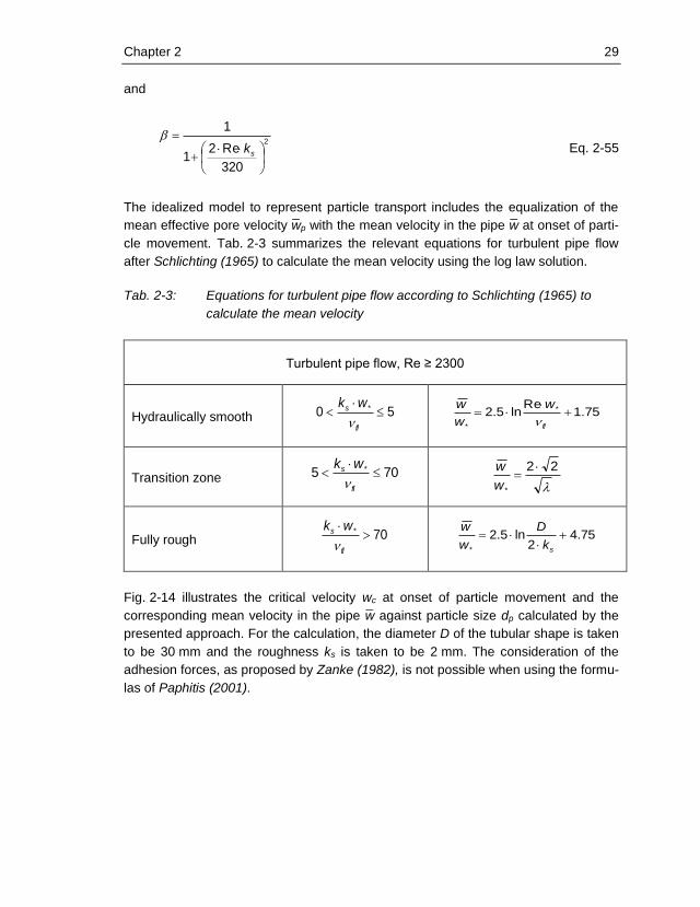
The idealized model to represent particle transport includes the equalization of the
mean effective pore velocity w̄p with the mean velocity in the pipe w̄ at onset of parti-
cle movement. Tab. 2-3 summarizes the relevant equations for turbulent pipe flow
after Schlichting (1965) to calculate the mean velocity using the log law solution.
Tab. 2-3: Equations for turbulent pipe flow according to Schlichting (1965) to
calculate the mean velocity
Turbulent pipe flow, Re ≥ 2300
Hydraulically smooth 50 *
fl
s wk
75.1
Reln5.2 *
*
fl
w
w
w
Transition zone 705 *
fl
s wk
22
*
w
w
Fully rough 70*
fl
s wk
75.4
2ln5.2
*
sk
D
w
w
Fig. 2-14 illustrates the critical velocity wc at onset of particle movement and the
corresponding mean velocity in the pipe w̄ against particle size dp calculated by the
presented approach. For the calculation, the diameter D of the tubular shape is taken
to be 30 mm and the roughness ks is taken to be 2 mm. The consideration of the
adhesion forces, as proposed by Zanke (1982), is not possible when using the formu-
las of Paphitis (2001).

30 Chapter 2
Fig. 2-14: Critical velocity wc at onset of particle movement and mean velocity in
the pipe w̄ against particle size dp
In through-flowed porous media usually only the filter velocity and the average veloci-
ty can be measured. However, since the idealized model to represent particle
transport considers the pore velocity wp, the filter velocity or average velocity must be
converted into pore velocity by using Eq. 2-17.
2.2 Instrumentation of embankment dams
2.2.1 General
An important aspect of the safety of dams is monitoring and surveillance. Individually
adapted measuring devices and monitoring systems together with visual inspection
allow a comprehensive assessment of the safety of a dam. According to ANCOLD
(2003) dam monitoring is the observation of measuring devices that provide data
from which can be deduced the performance and the behavioural trends of a dam
and its appurtenant structures and the recording of such data. Surveillance is the
continuing examination of the condition of a dam and its appurtenant structures, the
review of operation, maintenance and monitoring procedures and results in order to
determine whether a hazardous trend is developing or appears likely to develop.
Dam monitoring is carried out with the aim to provide confirmation of the design as-
1.00E-03
1.00E-02
1.00E-01
1.00E+00
1.00E+01
1.00E+02
1.00E+03
0.001 0.01 0.1 1 10
velo
city
w [
cm/s
]
Particle diameter dp [mm]10-3 10-2 10-1 100 101
101
10-5
10-4
10-2
10-1
100
Particle size dp [mm]
Vel
oci
tyw
[m/s
]
Laminar flowTransition –
turbulent flow
Critical velocity wc
10-3
Average velocity w

Chapter 2 31
sumptions and predictions of performance during the construction phase, the first
impounding and operational life. In addition, it is necessary to detect any signs of
abnormality or unsafe trends in the behaviour of the dam and its foundation while it is
subjected to the applied loading and to intervene promptly. The analysis of the ob-
tained data also allows developments in dam engineering through better understand-
ing of material properties such as rockfill modulus in CFRDs (Hunter and Fell, 2003),
checking of analytical methods and new construction materials, such as asphaltic
concrete cores and geomembranes. Dam monitoring is also absolutely indispensible
during and after raising or remedial works, to ensure that the additional loading intro-
duced by the new works, is applied in a manner which will not adversely affect the
safety of the dam.
In the following, the main points of dam monitoring are summarized. Detailed infor-
mation on the topic is given amongst others in STK (2006, 2005) and DWA (2008).
2.2.2 Monitoring concept
Each dam is unique, in regards to its design, construction and conditions specific to
the site, in particular those related to its foundation. This has to be considered in the
type and scope of the monitoring concept. Therefore the monitoring system is de-
signed in a way that it is possible to measure both the external loads and effects from
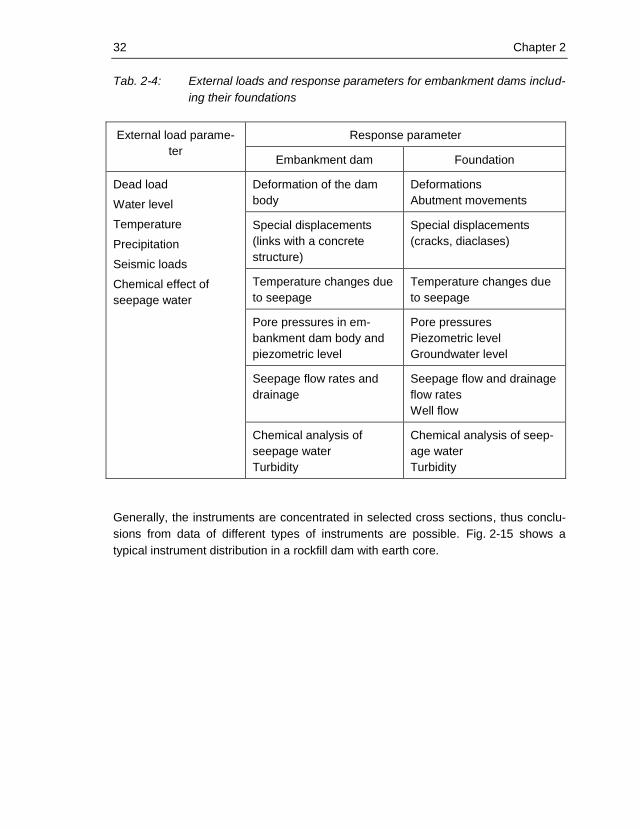
the surroundings as well as the response parameters. Tab. 2-4 summarizes the most
important external loads and response parameters for embankment dams including
their foundations.
The selection of the measuring method and the measuring system is determined by
the measuring target. Generally the measuring target is specified, taking into account
normal operation conditions and extreme operation conditions, and then it is decided
which measuring method and measuring system can achieve this best. Additionally
the selected measuring systems should meet the requirements and resistance to
external influences.
32 Chapter 2
Tab. 2-4: External loads and response parameters for embankment dams includ-
ing their foundations
External load parame-
ter
Response parameter
Embankment dam Foundation
Dead load
Water level
Temperature
Precipitation
Seismic loads
Chemical effect of
seepage water
Deformation of the dam
body
Deformations
Abutment movements
Special displacements
(links with a concrete
structure)
Special displacements
(cracks, diaclases)
Temperature changes due
to seepage
Temperature changes due
to seepage
Pore pressures in em-
bankment dam body and
piezometric level
Pore pressures
Piezometric level
Groundwater level
Seepage flow rates and
drainage
Seepage flow and drainage
flow rates
Well flow
Chemical analysis of
seepage water
Turbidity
Chemical analysis of seep-
age water
Turbidity
Generally, the instruments are concentrated in selected cross sections, thus conclu-
sions from data of different types of instruments are possible. Fig. 2-15 shows a
typical instrument distribution in a rockfill dam with earth core.

Chapter 2 33
Fig. 2-15: Typical monitoring for earth core rockfill dam
2.2.3 Loads and effects from the surrounding environment
Dead load as well as loads and effects from the surrounding environment directly
affect the dam. The water pressure and seepage forces caused thereby are the deci-
sive forces that act on a dam. Therefore, each dam must have at least one measur-
ing device for monitoring the water level. Automated systems, such as pneumatic
gauges or sonar gauges are used to measure the water level in addition to the com-
monly used staff gauges.
Atmospheric conditions such as temperature, humidity and precipitation are important
data as well. For example, the amount of rain or melting snow can affect most hy-
drometric measurements such as amount of seepage water, pore pressure and
ground water, and therefore have to be included in the data evaluation and analysis
of the monitoring data. The climatic conditions are usually obtained from a meteoro-
logical station which is located in the vicinity of the dam. The use of data from weath-
er stations which are not in the immediate vicinity of the dam is only useful if the
transfer and representation of values are guaranteed.
In areas with seismic activities, the installation of seismographs to record the seismic
Geodetic survey point
Hydraulic overflow settlement gauge
Vertical settlement gauge
Seepage measuring point
Piezometer (pressure cell)
Standpipe
34 Chapter 2
conditions may be required. Ground motion caused by tectonic movement or induced
by impounding of the reservoir can thus be captured in terms of time and intensity. By
placing one seismograph at the dam crest and another one at the dam heel, it is also
possible to draw conclusions on the change of ground acceleration over the height of
the dam.
2.2.4 Response parameters
2.2.4.1 Seepage
The hydraulic pressure provokes seepage through the dam and its foundation, since
the materials used for construction are more or less permeable. Therefore, seepage
data are an important indicator of dam performance. By observing the location, quan-
tity and quality of seepage emerging from the dam and its foundation and particularly
the deviations from the normal state, one can get early warning of problems which
may jeopardize the safety of the dam such as internal erosion in the dam and its
foundation as well as increased pore pressures.
Generally the seepage rate varies according to the reservoir elevation, but precipita-
tion and the melting of snow can also influence the measurements. The total water
discharge rate gives an indication of the global behaviour of the sealing elements. It
is preferable to collect the seepage close to the downstream toe of the sealing ele-
ment and to isolate areas from each other, so the readings are not influenced exces-
sively by flow through the rockfill zones and runoff from the abutments. This proce-
dure allows, in the case of anomalies, to localize the critical zone and to facilitate the
determination of the origin of the seeping water.
The discharge rate of seepage and drainage at the outlet is generally measured by
timed discharge into a measuring vessel or by a calibrated weir. Measurements of
the water quality (turbidity, chemical analysis) may also be useful to detect the con-
tent of fine particles and dissolved materials. However, it is often impractical or im-
possible to collect and measure all seepage, especially for dams on alluvial founda-
tions. Problems also are experienced when the toe of the dam is below the tailwater
level. In these cases, the data of the piezometers installed in the foundation under
and downstream of the dam can give information on changing conditions which might
indicate a problem developing.
These classical methods for seepage collection and monitoring are normally installed
during construction and it may not be possible to install afterwards.
Chapter 2 35
2.2.4.2 Pore pressure
In an embankment dam, it is important to check the evolution of pore pressures,
especially in the core and the foundation. Generally pore pressures vary with reser-
voir level. During construction and first years of operation, pore pressures in clay
cores also vary with the degree of consolidation. Additionally, dynamic loading, e.g.
earthquakes, may induce and increase pore pressures. Provided there is adequate
coverage along the dam, the pore pressure data of the embankment and the founda-
tion can give vital quantitative information for use in assessing the slope stability,
potential “heave” conditions in foundations and for identifying unusual seepage pres-
sure, which may be a precursor to internal erosion and piping. For a slope the factor
of safety against sliding is very sensitive to the pore pressures, and so they are
closely observed to ensure that they not exceed the values allowed for the project.
This is particularly important for dams with inclined cores or large reservoir fluctua-
tions.
For the analysis and evaluation of pore pressure measurements for each monitoring
cross section the measured pore pressures are plotted against the water level in the
reservoir. Correlation and regression analyses are especially helpful for a more de-
tailed analysis of data obtained from measurements of pore. It is also possible to
determine the response time of the pore pressure sensors on changes in the reser-
voir’s water level by using correlation functions (Muckenthaler, 1989). In general, for
intact sealing elements, the correlation between pore pressure and reservoir level
decreases from upstream to downstream and thus provides information on the effec-
tiveness of the sealing elements. If sufficient piezometers are placed in a monitoring
cross section, for each reservoir level, the corresponding flow net can be determined
by using the measured pore pressures.
Pore pressures in the embankment or the foundation are generally measured by
placing pneumatic, hydraulic or electrical pressure cells. Therefore, they provide only
punctual information. A detailed discussion on advantages and disadvantages of
each type is given in Fell et al. (2005). There is also an on-going discussion if pie-
zometers should be installed in the cores of earth and rockfill dams. The tubes or
wires leading to the measuring gauge are laid in trenches, which leaves a potential
weakness in the dam from internal erosion and piping perspective. High gradients
may occur from the upstream face of the core to the first piezometer and may initiate
internal erosion or piping along the trenches. However, long-term trends in pore
pressures are valuable in assessing slope stability and potential piping problems. To
minimize the risk of internal erosion and piping problems, the USBR (1987) recom-
mends installing the piezometers in the core, but not too close to its upstream face
and to backfill the trenches with well compacted dry mixture of bentonite and filter
36 Chapter 2
sand.
2.2.4.3 Surface displacement
Geodetic survey points are installed on almost every dam. Regular accurate meas-
urements of the surface displacement are useful as a check on design assumptions
and as an indication of developing problems such as marginal slope stability and
internal deformations due to softening or internal erosion and piping in the embank-
ment or the foundation. Their vertical and horizontal positions are periodically deter-
mined by accurate surveys by means of reference to fixed monuments and bench-
marks located outside the dam and the reservoir’s area of influence. The movement
vectors obtained from the vertical and horizontal displacements often give a good
indication of the mechanism causing the displacement.
Generally, the geodetic survey points are positioned centrally along the crest and on
the upstream and downstream slopes, because markedly different movements occur
between the dam core and adjacent filter and rockfill zones. They are also installed at
transitions to concrete structures because this is where local seepage, softening and
abnormal deformation is often a guide to developing problems. When necessary the
survey is extended to the surrounding areas to detect slope instabilities caused by
the impounding of the reservoir. The displacements are measured by using geodeti-
cal methods, such as traverse and levelling.
2.2.4.4 Displacement and deformation
In contrast to the determination of surface displacement by means of geodetic meas-
urements internal displacement and deformation measurements are often carried out
only on larger earth, earth and rockfill dams and on concrete face rockfill dams (Fell
et al., 2005). The measurements are particularly useful for monitoring the long-term
settlement of the dam and foundation in order to confirm the design assumptions or
to detect any sign of abnormality or unsafe trends.
Monitoring of deformations within the dam body is generally based on a network of
instruments which are concentrated in cross sections. Vertical and horizontal dis-
placements and deformations are measured using vertical plate gauges, slope indi-
cators and extensometers which are either embedded in the fill as the dam is con-
structed, or installed in boreholes. On some larger dams the horizontal plate gauges
are sometimes embedded in the dam fills as the dam is constructed. Their use is
often combined with hydraulic settlement gauges, so that a settlement profile can be
determined.
While these instruments provide useful information on dam deformations, it is disput-
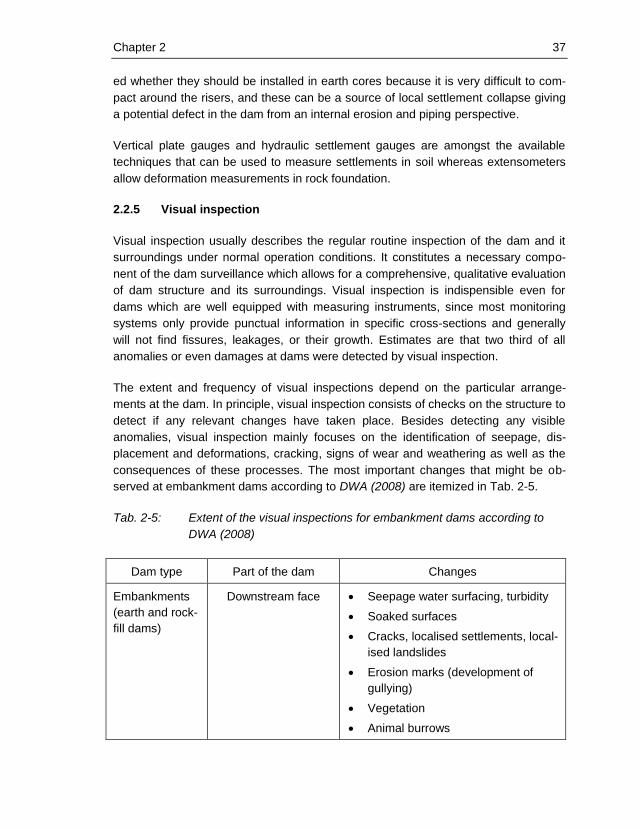
Chapter 2 37
ed whether they should be installed in earth cores because it is very difficult to com-
pact around the risers, and these can be a source of local settlement collapse giving
a potential defect in the dam from an internal erosion and piping perspective.
Vertical plate gauges and hydraulic settlement gauges are amongst the available
techniques that can be used to measure settlements in soil whereas extensometers
allow deformation measurements in rock foundation.
2.2.5 Visual inspection
Visual inspection usually describes the regular routine inspection of the dam and it
surroundings under normal operation conditions. It constitutes a necessary compo-
nent of the dam surveillance which allows for a comprehensive, qualitative evaluation
of dam structure and its surroundings. Visual inspection is indispensible even for
dams which are well equipped with measuring instruments, since most monitoring
systems only provide punctual information in specific cross-sections and generally
will not find fissures, leakages, or their growth. Estimates are that two third of all
anomalies or even damages at dams were detected by visual inspection.
The extent and frequency of visual inspections depend on the particular arrange-
ments at the dam. In principle, visual inspection consists of checks on the structure to
detect if any relevant changes have taken place. Besides detecting any visible
anomalies, visual inspection mainly focuses on the identification of seepage, dis-
placement and deformations, cracking, signs of wear and weathering as well as the
consequences of these processes. The most important changes that might be ob-
served at embankment dams according to DWA (2008) are itemized in Tab. 2-5.
Tab. 2-5: Extent of the visual inspections for embankment dams according to
DWA (2008)
Dam type Part of the dam Changes
Embankments
(earth and rock-
fill dams)
Downstream face Seepage water surfacing, turbidity
Soaked surfaces
Cracks, localised settlements, local-
ised landslides
Erosion marks (development of
gullying)
Vegetation
Animal burrows

38 Chapter 2
Dam type Part of the dam Changes
Dam crest Cracks, localised settlements
Erosion marks
Vegetation
Animal burrows
Condition of the road
line of sight - check horizontal &
vertical
Upstream face (ac-
cessible section)
Vortex formation on the water sur-
face
Cracks, localised settlements de-
formations, localised landslides
Bulging of surface sealing elements
Damage on the surface sealing
element
Displacement of riprap
Vegetation
Animal burrows
Inspection gallery Cracks
Leaking seepage water, turbidity
Sinter formations
Condition of concrete
Clogging of drainage system
Contact between
embankment and
concrete structures or
rock foundation
Relative displacements
Localised settlement
Leaking of seepage water
2.3 Internal erosion in embankment dams
2.3.1 General
Even for newly constructed dams, internal erosion due to unforeseen and undetected
flow through the embankment or the foundation still poses a risk which should not be
underestimated. An analysis of published data on dam failure and accidents by the

Chapter 2 39
research group led by R. Fell (Foster, 1999, Foster et al., 2000a, Foster et al., 2000b)
showed that internal erosion has historically resulted in about 0.5% embankment
dam failing and about 1.5% experiencing an accident. Most of the failures occurred in
homogeneous earth fill dams, however, central core earth and rockfill dams made up
about 25% of the accidents.
2.3.2 Mechanism of failure
Based on field and laboratory studies, Fannin and Garner (2010) conclude that the
presence of three factors are likely to determine the form and extent of internal ero-
sion processes. These factors may be considered to represent adverse conditions or
weakness within the dam body and foundation, identified as material susceptibility,
critical stress and hydraulic load. To illustrate how the three factors can interact,
Fannin and Garner (2010) propose the Venn-diagram given in Fig. 2-16. The different
overlapping areas represent different failure mechanism.
As it can be observed in Fig. 2-16, internal erosion requires that in the dam body or
the foundation critical flow conditions are present or can develop which cause de-
tachment and transport of soil particles. Fig. 2-17 illustrates in an exemplary fashion
an earth core rockfill dam with a cut off wall to control foundation seepage where
critical flow conditions can occur. Depending on the design of the dam and the soil
materials used, as well as on the topography and geology of the dam site, the areas
of critical flow conditions can vary.
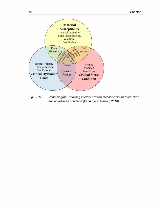
40 Chapter 2
Fig. 2-16: Venn diagram, showing internal erosion mechanisms for three over-
lapping adverse condition (Fannin and Garner, 2010)
Material
SusceptibilityInternal Instability
Filter Incompatibility
Void Space
Free Surface
Arching
Vibration
Low Stress
Critical Stress
Condition
Seepage Velocity
Hydraulic Gradient
Pore Pressure
Critical Hydraulic
Load
Fines
Migration
Soil
Distress
Hydraulic
Fracture
Heave
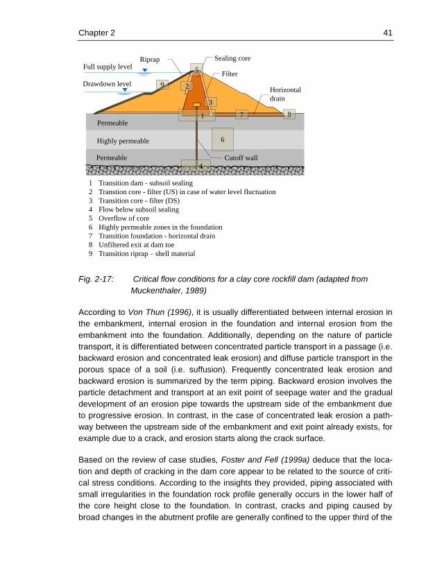
Chapter 2 41
Fig. 2-17: Critical flow conditions for a clay core rockfill dam (adapted from
Muckenthaler, 1989)
According to Von Thun (1996), it is usually differentiated between internal erosion in
the embankment, internal erosion in the foundation and internal erosion from the
embankment into the foundation. Additionally, depending on the nature of particle
transport, it is differentiated between concentrated particle transport in a passage (i.e.
backward erosion and concentrated leak erosion) and diffuse particle transport in the
porous space of a soil (i.e. suffusion). Frequently concentrated leak erosion and
backward erosion is summarized by the term piping. Backward erosion involves the
particle detachment and transport at an exit point of seepage water and the gradual
development of an erosion pipe towards the upstream side of the embankment due
to progressive erosion. In contrast, in the case of concentrated leak erosion a path-
way between the upstream side of the embankment and exit point already exists, for
example due to a crack, and erosion starts along the crack surface.
Based on the review of case studies, Foster and Fell (1999a) deduce that the loca-
tion and depth of cracking in the dam core appear to be related to the source of criti-
cal stress conditions. According to the insights they provided, piping associated with
small irregularities in the foundation rock profile generally occurs in the lower half of
the core height close to the foundation. In contrast, cracks and piping caused by
broad changes in the abutment profile are generally confined to the upper third of the
1 Transition dam - subsoil sealing
2 Transtion core - filter (US) in case of water level fluctuation
3 Transition core - filter (DS)
4 Flow below subsoil sealing
5 Overflow of core
6 Highly permeable zones in the foundation
7 Transition foundation - horizontal drain
8 Unfiltered exit at dam toe
9 Transition riprap – shell material
6
2
3
4
7 81
5Full supply level
Drawdown level
Sealing core
Filter
Horizontal
drain
9
Cutoff wall
Riprap
Permeable
Highly permeable
Permeable

42 Chapter 2
height of the dam where tensile stresses might be expected. Cracks associated with
arching of narrow or soft cores between the shell zones and hydraulic fracturing are
most likely to occur within middle third of the dam height.
In Fig. 2-18 and Fig. 2-19 typical crack patterns due to differential settlements are
shown.
Fig. 2-18: Typical cracks in central cores after (Sherard et al., 1963) and
(Thomas, 1976)
Fig. 2-19: Typical transverse differential settlement cracks (Sherard et al., 1963)
For a better understanding of internal erosion in the embankment and the foundation,
according to (Foster and Fell, 1999b), it is helpful to break up the failure mechanism
into four phases, which are initiation, continuation, progression and breach. Fig. 2-20
RockSand
(dense)Clay lense
(very compressible)
Open cracks
Settlement of crest
(exaggerated)Settlement of crest
(exaggerated)
Rock
Shear crack
Settlement of crest
(exaggerated)
Open cracks
Open cracks
Open Cracks
Open crack
Longitudinal section
Plan view
Longitudinal section
Plan view

Chapter 2 43
shows the development of failure for concentrated leak erosion (a), backward erosion
(b), piping from the embankment to the foundation (c) and piping through the founda-
tion (d).
(Foster, 1999) and (Foster and Fell, 1999b) provide a comprehensive overview of the
factors and conditions that influence the onset and the further development of inter-
nal erosion leading to failure of a dam. They are briefly summarized in the following.
The onset of internal erosion in the dam or the foundation requires, beside the critical
hydraulic load that either soils susceptible to suffusion are present or that filter in-
compatibility or local defects provoke piping. Typical examples of local defects are,
amongst others, continuous cracks caused by differential settlement, hydraulic frac-
turing, earthquake or shrinkage, areas of high permeability due to poor compaction or
segregation as well as open joints and cracks in the foundation and concrete struc-
tures. Depending on failure mechanism, the critical hydraulic load can be character-
ised as follows: In the case of suffusion, the drag force caused by the seepage must
be large enough to transport the fine particles through the pore system of the coarser
particles. For piping to occur, the hydraulic shear stress must be greater than the
critical shear stress of the soil to detach and transport the particles.

44 Chapter 2
Fig. 2-20: Model for development of failure (Foster, 1999)
The continuation of the erosion process will depend largely on whether particle
transport can be controlled by effective filter zones or not. Therefore in state of the art
embankment dams, filter layers are arranged in the embankment where critical flow
conditions are likely to occur. If these filters are designed and constructed according
to modern filter criteria, such as (Sherard et al., 1984) or (USBR, 1999), the internal
erosion process will almost certainly grind to a halt at an early stage. If the arranged
filters do not meet the design criteria, erosion may continue and, depending on the
grading of the filters and the soil, some, excessive or continuing erosion may occur
(Foster and Fell, 1999a).
Initiation Continuation Progression Breach/failure
Leakage exits on
downstream side of
core and backward
erosion initiates
Continuation of erosion Backward erosion
progresses to form a pipe
Breach mechanism
forms
Initiation Continuation Progression Breach/failure
Leakage exits the
core into the
foundation and back-
ward erosion initiates
as core erodes into the
foundation
Continuation of erosion Backward erosion pro-
gresses to form a pipe.
Eroded soil is transported
in the foundation
Breach mechanism
forms
Initiation Continuation Progression Breach/failure
Concentrated leak
forms and erosion
initiates
Continuation of
erosion
Enlargement of the
erosion pipe
Breach mechanism
forms
Initiation Continuation Progression Breach/failure
Leakage exits from
the foundation and
backward erosion
initiates
Continuation of
erosion
Backward erosion
progresses to form a
pipe
Breach mechanism
forms
a)
b)
c)
d)
Chapter 2 45
The progression of the erosion process requires that the critical hydraulic load for
particle detachment and particle transport is still present. Furthermore, it depends on
the likelihood and rate of pipe enlargement and whether the pipe will collapse,
whether upstream zones may control the erosion process by flow limitation and
whether a pipe will extend through the low permeability zones of the embankment
(Fell and Fry, 2007). In cases where the ability of the soil to support the roof of the
pipe is not given, the pipe will collapse and the progression of erosion may stop due
to reduction or prevention of flow. Surface sealings and crack filling from fine grained
upstream zones such as random fill material may contribute to flow limitation. Apart
from that, without any intervention, the process can only stop if the reservoir level
drops due to the outflow resulting in a lower hydraulic gradient.
Possible failure mechanisms caused by internal erosion include large seepage flows
associated with gross enlargement of the erosion pipe, crest settlements or sinkholes
leading to overtopping as well as high pore pressures downstream causing slope
failure. All these failure mechanisms ultimately result in emptying of the dam storage
in a fast, uncontrolled manner.
2.3.3 Time for development of internal erosion
At the University of New South Wales methods have been developed along with the
research activities on internal erosion in dams that allow the estimation of time for
development of internal erosion (Fell et al., 2001) and the probability of failure (Fell et
al., 2004), (Fell and Wan, 2005).
The information on the rate of process of the different types of internal erosion is
based primarily on a comprehensive review of published data on dam failures and
accidents caused by internal erosion. Additionally, results of laboratory tests, carried
out to determine the erosion resistance and erosion rate of soils used in dam con-
struction, were considered. Basically the method assumes that the rate of process of
an erosion mechanism is correlated to the likelihood this mechanism will happen.
Accordingly, for each type of internal erosion the different phases as well as the me-
chanics of the process and the factors, which affect the likelihood of the process
occurring, are taken into account. The resulting rates of process for the different
types of internal erosion are qualitative and can be classified according to Tab. 2-6.

46 Chapter 2
Tab. 2-6: Qualitative term for times of development of internal erosion, piping
and breach after Fell et al. (2001)
Qualitative term Equivalent time
Slow Weeks or months, even years
Medium Days or weeks
Rapid Hours (>12 hours) or days
Very Rapid < 3 hours
The data compiled in (Fell et al., 2001) suggests that the rate of process for internal
erosion due to concentrated leaks, zones of high permeability and hydraulic fracture
is rapid or very rapid, once the reservoir level reaches the crack or the zone of high
permeability or the level at which hydraulic fracture is induced. In contrast, for back-
ward erosion, the rate of process is rather slow until the erosion pipe breaks through
to the reservoir. However, after formation of a continuous tunnel between the up-
stream and downstream sides of the embankment or its foundation, the process may
develop rapidly for soils with the ability to hold the roof of the pipe. Assuming that
open joints or cracks in the foundation or conduits are not wide, internal erosion is
likely to develop slowly. In the case of suffusion the rate of process is slow since the
failure mechanism involves a gradual migration of fines within the soil.
2.3.4 Detectability of internal erosion
In general, it is not entirely excluded that detection of internal erosion during the
initiation phase or continuation phase may be possible with the conventional monitor-
ing systems so far used for dam monitoring. However, because of the used monitor-
ing systems and strategies, detection of internal erosion during the progression
phase or just before failure of the dam is much more likely. Precursors or signs of
possible erosion processes are an increase in seepage, turbidity of the seepage
water as well as sinkholes and settlements at the crest or the slope.
In many cases the inability to detect that internal erosion has initiated relates closely
to the mechanisms of initiation (Fell et al., 2001). Usually the increase in seepage
water or change in pore pressure during early stages of the internal erosion process
is not sufficient to identify conclusively that internal erosion takes place. For example,
in the case of initiation of internal erosion by a concentrated leak, it will be very un-

Chapter 2 47
likely that piezometers will be located where a leak occurs. However, it is generally
agreed that monitoring of seepage behaviour is the most likely means to identify that
internal erosion has occurred. The seepage monitoring system should be set up in a
way that it allows separate collection of seepage water from different portions of the
dam. Additionally, the option should be provided to separate out the effects of rainfall
or snowmelt on the amount of seepage water.
2.4 Geophysical methods for detection of internal erosion
2.4.1 General
Today, a variety of geophysical methods can be employed to investigate seepage in
embankment dams with the goal to facilitate early detection of anomalous seepage,
piping and internal erosion. A summary of the most common used methods can be
found in Armbruster et al. (1989) and Lum and Sheffer (2010). In the following pages,
methods that are generally considered to be the most promising investigation and
monitoring tools to detect leakage and internal erosion are described.
2.4.2 Self-potential method
The self-potential technique is a cost effective geophysical method to investigate
internal seepage in embankment dams, which has been frequently used (e.g. Ogilvy
et al. 1969; Butler 1989; Rozycki et al. 2006). Self-potential methods measure natu-
ral-earth electrical potentials in the dam body. One source of these self-potentials is
the streaming potential or electro kinetic potential, which arises from the flow of fluid
through porous media.
As water flows through a capillary system, it collects and transports positive ions from
the surrounding materials. The positive ions accumulate at the exit point of the capil-
lary, leaving a net positive charge. The uncollected negative ions accumulate at the
entry point of the capillary, thus leaving a net negative charge. If the streaming poten-
tials developed by this process are of sufficient magnitude to measure, the entry point
and the exit point of zones of concentrated seepage can be determined due to the
negative and positive self-potential anomalies.
Self-potential surveys are conducted by measuring electrical potential differences
between pairs of non-polarizable electrodes embedded in the dam body. The field
procedure consists of placing one electrode (base electrode) at a point distant from
the expected anomalous activity. Another electrode is moved at selected intervals in
the area of interest, and the potential between the base electrode and the moving
electrode is measured and recorded at each location. Where anomalies are ob-
served, detailed measurements are made at small intervals to better define the limits

48 Chapter 2
of these anomalous zones.
Self-potential data interpretation can range from a simple qualitative inspection of the
plotted self-potential profiles to complex computer modelling involving interactions
between temperature, electrochemical reactions and dam / foundation geometry.
Data are plotted as profiles or, if the data provide sufficient areal coverage, as con-
tour plots. All other points will be equal. The anomaly location corresponds to the
point of seepage flow. There are several other sources of self-potential variations that
may act as noise or interference when mapping streaming potential for a seepage
investigation. These include buried metal, temperature variations, soil property varia-
tions, electrochemical variations, topographic effects and tellurics.
2.4.3 Resistivity method
Electrical resistivity survey is another non-invasive geophysical method to investigate
internal seepage in embankment dams. Valuable experience has been gained from
research and field installations carried out in Sweden since 1993 (Johansson and
Dahlin 1996; Johansson et al. 2005; Sjödahl et al. 2010). In the resistivity method, an
electrical current is introduced into the ground and the resulting potential distribution
is measured.
Electrical resistivity surveying is based on the principle that the distribution of electri-
cal potential in the ground around a current carrying electrode depends on the elec-
trical resistivities and distributions of the surrounding soils and rocks (Zhang, 2004).
Since electrical resistivity of soils and rocks correlates with other soil / rock proper-
ties, such as clay content, groundwater conductivity, soil porosity and degree of water
saturation, seepage condition of the dam can be inferred.
Electrical resistivity techniques may be used in two different modes. Firstly, vertical
electrical sounding, VES, is using the same midpoint for a specific electrode configu-
ration. By systematically increasing the electrode separation, the current is forced
deeper into the subsurface and the resistivity for different depths on a given location
is the result. The other mode is electrical profiling, where the midpoint is varied and
all electrode separations are fixed. The result in this case is resistivities on the same
depth along a line. Combining soundings and profiling will give a collection of meas-
urements on different depths along a line. This procedure is often referred to as con-
tinuous vertical electrical sounding, CVES.
Instrument readings (current and voltage) are generally reduced to “apparent resistiv-
ity” values. The apparent resistivity is the resistivity of the homogeneous half-space
which would produce the observed instrument response for a given electrode spacing
(profiling). Apparent resistivity is a weighted average of soil resistivities over the
Chapter 2 49
depths of investigation. For soundings, a plot of apparent resistivity versus electrode
spacing (sounding curve) is obtained.
Resistivity data are generally interpreted using the modelling process. A hypothetical
model of the dam / foundation and its resistivity structure is generated. The theoreti-
cal electrical resistivity response over that model is calculated and the result com-
pared with the observed field response. If differences are noted between observed
and calculated response, the hypothetical earth model will be adjusted until the cal-
culated response nearly fits with the observed data. Resistivity models are generally
not unique, i.e., a large number of earth models can produce the same observed
data or sounding curve. In general, resistivity methods determine the conductance of
a given stratigraphic layer or unit. The conductance is the product of the resistivity
and the thickness of the layer. Hence, the layer could be thinner and more conduc-
tive or thicker and less conductive, while producing essentially the same results.
Hence constraints on the model, from borehole data or assumed unit resistivities, can
greatly enhance the interpretation.
2.4.4 Temperature measurements
Temperature measurements are indirect means to determine the presence, location
and quantity of seepage flows through dams. Both surface water temperature and
ground temperature show seasonal variation. Due to the low thermal conductivity of
soil and other construction materials, significant differences between the temperature
of the reservoir water and the temperature distribution within the dam can develop.
The advective heat transport associated with reservoir water flowing into the dam
through a leak in the sealing element or a zone of higher permeability will lead to a
distortion of the temperature distribution within the dam towards the reservoir water
temperature.
Temperature measurements have long been considered to be useful for leakage
detection in embankment dams (e.g. Kappelmeyer 1955; Armbruster et al. 1993;
Johansson 1997; Dornstädter and Aufleger 1998) . The measurements can be punc-
tual or distributed. Punctual measurements can be achieved by installed temperature
sensors, which are placed for this reason only. Several pressure sensors also include
temperature sensors for temperature compensation, and provide an easy possibility
of retrieving temperature data. Vertical temperature profiles can be obtained by using
the temperature sounding method. To insert the temperature sensors, existing stand-
pipes can be used, or new standpipes can be rammed or drilled into the dam (e.g. at
the crest, at the toe of the dam, or in the filters) to the required depth. Measurements
are conducted using a portable temperature probe, which can be lowered to different
depths or by installing a sensor chain comprising several temperature sensors at
50 Chapter 2
distinct intervals for permanent monitoring (Dornstädter, 1997). Distributed fibre optic
temperature measurements (DFOT) can be performed by means of a fibre optic
cable installed at specific locations along or across the dam. Such a distributed sen-
sor can be installed during the construction of the dam or as part of a re-
instrumentation program at easily accessible sections of the dam. The main ad-
vantage of this kind of temperature sensors is that the entire length of the dam can
be monitored with a spatial resolution of 1.0 m.
Leakage detection by means of temperature measurements have been typically
implemented through two major approaches. Firstly the passive method (Kappel-
meyer 1955; Armbruster et al. 1993; Johansson, 1997), which employs temperature
as a tracer to detect anomalies in the flow field, and secondly the active method or
heat-up method (Dornstädter, 1997), which allows detecting the presence and
movement of water by evaluating the thermal response after external heat is induced.
Passive temperature method
The temperature within an embankment dam depends mainly on the natural tem-
perature in the upstream reservoir and in the air. These temperatures vary seasonally
and create temperature waves that propagate through the dam. Temperature gradi-
ents can exist in the form of permanent or seasonal temperature differences, as well
as in the form of significant temperature fluctuations at the probable source of seep-
age. If leakage is present, temperature anomalies will be transported into the struc-
ture by means of advection and will propagate throughout the earthen body, dis-
torting the temperature field. Distributed measurements allow for a precise localiza-
tion of the anomaly, delimiting quite precisely the area affected by leakage. This
method also allows determination of the source of the anomaly by contrasting the
abnormal temperature to the external temperature history. Magnitude and extent of
leakage can be estimated by means of the time lag and the intensity of the tempera-
ture anomaly at a given location. Whereas for localization of anomalies a single or
few measurements are sufficient, the quantification of leakage requires regular
measurements in reasonable short time intervals.
It is apparent that the passive method requires the presence of a temperature differ-
ence between the external boundaries (especially the temperature of the reservoir
water) and the sensor surroundings. When such conditions do not exist, the passive
method is not applicable and the active method may be used.
Active temperature method
Active methods were developed as a further step in the application of temperature
methods for seepage/leakage monitoring. The most common method is the Heat-up

Chapter 2 51
Method, developed upon DFOT, where heat is added by an electrical current into
copper wires built in alongside the optical fibre (Dornstädter, 1997). This approach is
based on the thermal response of the sensor surroundings to the additional heat,
which can indicate whether the cable is within a moist, a partially saturated or a fully
saturated medium, and whether a seepage flow is present or not. In principle, the
heat input causes a temperature rise along the cable. In the case of unsaturated
surroundings of the sensor, the temperature increase depends on the surrounding's
thermal conductivity and, thus, on the moisture content. High moisture contents
around the sensor enhance conductive heat transport, causing a lower temperature
rise at these sections of the cable. In the case of the presence of seepage flows,
forced convection effects, that dissipate the additional heat more effectively, cause
lower temperature rises than in the conduction dominated cases.
Installations using active methods (heating or cooling) only provide information on the
direct surrounding of the sensor, but can be applied without local or seasonal tem-
perature variations present (e.g. under surface sealing). The heat-up method can be
used downstream of sealing elements or at the dam toe. In case of a central sealing
element it can even be used upstream of the sealing element. It can also be applied
to detect leakages through thin sealing elements such as membranes, asphaltic
linings or concrete slabs, by placing the sensor directly underneath them. The cable
should be located in such a way that it intercepts potential leakage flows, and can be
installed either in new structures or after refurbishment of such linings. The heat-up
method provides detailed information about the seepage regime on the close sur-
rounding of the sensor.
2.4.5 Other methods
Furthermore, ground penetrating radar (GPR) systems (Carlsten et al., 1995), seis-
mic methods (Vazinkhoo and Gaffran, 2002, Gaffran and Jeffries, 2005), and more
recently controlled source – audio frequency domain magnetics (CS-AFDM)
(Hughes, 2010) have been used to investigate the seepage behaviour of embank-
ment dams. A more detailed description of these geophysical methods is omitted
here and it is referred to in the quoted literature.

52 Chapter 2
Chapter 3 53
3 Distributed fibre optic measurements in embankment dams
3.1 General
Distributed fibre optic sensors provide the possibility of measuring temperature and
strain as a continuous profile along a single optical fibre. This unique feature that has
no match in conventional sensing techniques makes distributed fibre optic sensing
particularly interesting for the monitoring of large structures such as dams. Distribut-
ed fibre optic temperature sensing (DTS) has been successfully used for dam moni-
toring during the last 15 years (Johansson, 1997, Dornstädter and Aufleger, 1998,
Aufleger et al., 2005). This method is usually employed to detect and localize leakage
in embankment dams, and to monitor temperature development in large concrete
structures (Aufleger et al., 2007a).
Essential development of distributed temperature and strain sensing (DTSS) for
embankment dams has been made by Sensornet and Hydro Research (Johansson
and Watley, 2007). This technology is especially useful for monitoring internal parts
of a dam where single point, visual or geodetic monitoring methods are not able to
detect and localize differential deformations adequately.
3.2 Distributed fibre optic temperature measurements
3.2.1 Measuring system
Measuring principle
Optical fibres are made from doped quartz glass, which is a form of silicon dioxide
(SiO2) with an amorphous solid structure. Physical quantities, such as temperature,
or pressure and tensile forces induce lattice oscillations within the solid. The measur-
ing principle of distributed fibre optic temperature measurements is based on the fact
that after sending a light pulse from a powerful light source (laser) into a glass fibre, a
very small proportion of this light is backscattered at each point along a fibre
(Fig. 3-1). Unlike incident light, this scattered light, which is also called Raman scat-
tering, undergoes a spectral shift by an amount equivalent to the resonance frequen-
cy of the lattice oscillation (Raman effect). The light scattered back from the optical
fibre therefore contains three different spectral shares which are the Rayleigh scatter-
ing, the Stokes component and the anti-Stokes component (Fig. 3-2). The intensity of
the so-called anti-Stokes component is temperature dependent, while the so-called
Stokes component is practically independent of temperature. The local temperature
of the optical fibre is derived from the ratio of the anti-Stokes and Stokes light intensi-
ties and from the time the backscattered light takes to return to the detection unit.

54 Chapter 3
Fig. 3-1: Scattering of light inside a glass fibre
Fig. 3-2: Spectral components in the backscattered light
Measuring equipment
Distributed temperature sensing (DTS) systems are optoelectronic devices which
measure temperatures by means of optical fibres functioning as linear sensors. The
devices comprise all necessary components, such as the laser, the optical evaluation
unit and the computer for control and data acquisition. Temperatures are recorded
along the optical sensor cable, thus not at points, but as a continuous profile. A high
accuracy of temperature determination is achieved over great distances. Typically the
DTS systems can locate the temperature to a spatial resolution of 1 m with an accu-
racy of about ±1°C at a resolution of 0.01°C. Measurement distances of up to 30 km
can be monitored. However, temperature accuracy can be improved considerably
depending on calibration at the time of installation, and some specialised systems
can provide even tighter spatial resolutions.
Measuring cable
Returned
light
Light lost from the fibre
Scattering point
Incident
light
Frequency
Inte
nsi
ty
Ray
leig
h
scat
teri
ng
Ram
an
scat
teri
ng
Ram
an
scat
teri
ng
v0v0 - vR v0 + vR
Stokes fraction Anti-Stokes fraction

Chapter 3 55
Generally a type of optical fibre designed for data communication purposes is used
for distributed fibre optic temperature measurements. This optical fibre is referred to
as 50/125 multimode optical fibre. In a fibre optic cable several optical fibres are
usually combined in a plastic or metal tube, called a buffer tube. Typically either loose
tubes or tight tubes are used for the buffer tube. Depending on the type of the cable
and the material of the buffer tube, the tube is arranged centrically or twisted around
a central support element. For leakage detection using the heat-up method (Aufleger
et al., 2005), or for distributed filter velocity measurements (Perzlmaier, 2007), hybrid
fibre optic cables are used. In addition to the buffer tube with the optical fibres they
include electrical conductors, which allow heating by applying electrical voltage. The
structure of fibre optic cables aims to protect the optical fibres against external influ-
ences during manufacturing, laying and operation. In particular, it is necessary to
protect the fibre from water ingress, transverse compression, bending and elonga-
tion. Fig. 3-3 shows the cross section of a typical hybrid fibre optic cable.
Fig. 3-3: Sketch of standard hybrid cable
Quality of the measurement results
Since the ratio of the intensities of the Stokes and anti-Stokes component of the
Raman scattering is used to calculate the temperature at a point of the fibre, the
quality of the results of distributed fibre optic temperature measurements depends
highly on signal attenuation due to optical losses. The light pulse which is coupled
into the optical fibre is attenuated on its way through the medium of the fibre. Regard-
ing the attenuation, a differentiation can be made between intrinsic attenuation and
extrinsic attenuation. Intrinsic attenuation due to absorption and scattering occurs
when the light is travelling through the core of the optical fibre. Extrinsic attenuation is
caused by non-ideal modifications of the core cladding interface (CCI). In particular,
extrinsic attenuation is critical regarding the quality of distributed fibre optical temper-
ature measurements. A distinction is generally made between microbending and
Buffer tube
Central strength member
Water absorbent tape
Rip cord
Copper wire
Strain relief element
HDPE – outer jacket
Typical dia. 4 - 17 mm

56 Chapter 3
macrobending. Macrobending causes locally increased optical losses in highly
curved areas of the optical fibre. Due to sharp bends of the fibre axis, the incident
light meets the CCI at an angle larger than the critical anglec and a significant
part of the light will be lost into the cladding (see Fig. 3-4, left). Macrobending is gen-
erally caused by to small curvature radii or by crushing the cable during installation.
Microbending is normally seen where the CCI is not a smooth cylindrical surface.
Rather, due to processing or environmental factors (temperature, tensile forces), it
becomes modified or damaged as is shown in Fig. 3-4 (right). The uneven form of the
CCI results in exceeding of the critical angle c, and light is emitted from the core.
Fig. 3-4: Losses due to macrobending (left) and microbending (right)
3.3 Leakage detection and filter velocity measurements
3.3.1 General
Temperature measurements as a means to determine the presence, location and
intensity of seepage or leakage have already been introduced in subchapter 2.4.4. In
the following, some practical aspects and the theoretical background of distributed
filter velocity measurements are explained in more detail.
3.3.2 Heating of the fibre optic cables
The heat-up method requires adequate heat input along the cable for a certain time
interval. A.C or D.C. voltage produces the required continuous heat input if applied to
a conductor integrated in a hybrid fibre optic cable. By applying the voltage U on the
conductor with the electric resistance Rel, the current I is generated in the conductor.
The electric resistance Rel of a hybrid fibre optic cable is obtained by:
el
elel
A
LR
Eq. 3-1
Where el is the specific resistance of the conductor, L is the length of the conductor
CCI, damaged
light lost from the fibre core

Chapter 3 57
and Ael the conductor cross section. The generated heat flow q corresponds to the
rated power P of the power source and is the product of the voltage U and current I.
The heat input ql is the rated power divided by the length of the conductor and ac-
cordingly obtained from:
LR
U
L
IUq
el
l
2
Eq. 3-2
3.3.3 Theoretical background of distributed filter velocity measurement
This section gives a summary of the theoretical background of distributed filter veloci-
ty measurements that were developed by Perzlmaier (2007).
Heat transfer regimes
Heat transfer or heat transport is the transition of thermal energy due to temperature
difference. Heat transport always occurs from high to low temperature. Generally it is
differentiated between heat conduction, heat convection and thermal radiation. In
addition, heat transport may occur due to water vapour transport. The contribution of
the individual mechanisms of heat transfer in soil is mainly determined by its compo-
sition and structure and the degree of saturation. Fig. 3-5 provides an overview of the
predominant heat transfer mechanisms depending on particle size distribution and
degree of saturation.
Fig. 3-5: Predominant mechanism of heat transfer in non-through-flowed soil
after Farouki (1986)
Clay Silt Sand Gravel Stone
0
0.2
0.4
0.6
0.8
1.0
10-4 10-3 10-2 10-1 100 101 102
Equivalent particle diameter d10 [mm]
Deg
ree
of
satu
rati
on S
[-]
1 – thermally driven
redistribution of moisture
2 – thermally driven
water vapor diffusion
3 – free convection in pore water
4 – free convection in air
5 – thermal radiation
6 – conduction

58 Chapter 3
Heat conduction is the transfer of thermal energy through direct molecular communi-
cation within a medium or between mediums in direct physical contact. Characteristic
for conduction is that the heat transfer takes place without mass transportation. The
resulting heat flow q is proportional to the temperature gradient and the cross-
sectional area normal to the direction of heat flow. The proportionality factor is a
material-specific parameter which is called the thermal conductivity .
On the contrary, convection is heat transfer by mass motion of a fluid, when the
heated fluid is forced to move away from the source of heat carrying energy with it.
For natural or free convection, the fluid motion is generated by density differences in
the fluid occurring due to temperature gradients. In forced convection the fluid
movement results from pressure differences. A typical example of forced convection
is the transport of heat by flowing water.
Heat transfer by conduction takes place in all phases of the soil. In pore water, water
vapour and air free convection can occur due to temperature dependent changes in
density. Water vapour diffusion takes place only in unsaturated soils.
According to Fig. 3-5, in the case of non-through-flowed soils, vapour diffusion domi-
nates in clay and silt and free convection in gravel. Depending on the degree of satu-
ration, the convective flow occurs either in air or in pore water. Apart from that, pure
heat conduction prevails. Generally, heat transport by radiation can be neglected at
moderate temperatures (Frivik et al., 1977).
Substitution model for heat-up cables
Before heating, the temperature in the cable is equal to the temperature of the sur-
rounding material. The heating causes a rise in temperature inside the cable com-
pared to the temperature of the surrounding soil. The thermal behaviour of the heat-
up cable can be modelled using a substitutional system consisting of a core of infinite
thermal conductivity and a cable jacket of finite thermal conductivity (Fig. 3-6). By
using the substitutional system the increase in temperature dTint can be expressed as
surc dTdTdT int Eq. 3-3
where dTc is the temperature difference between the core and the cable jacket, and
dTsur is the temperature difference between cable jacket and the surrounding materi-
al.
Heat transport inside the cable is always heat conduction. With sufficient flow rate
through the soil, the temperature difference dTsur is determined by forced convection.
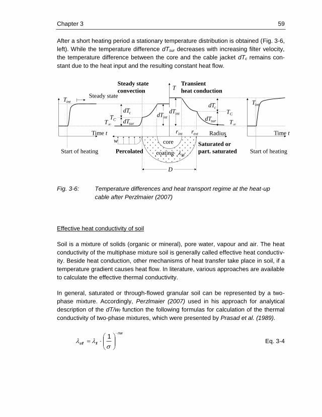
Chapter 3 59
After a short heating period a stationary temperature distribution is obtained (Fig. 3-6,
left). While the temperature difference dTsur decreases with increasing filter velocity,
the temperature difference between the core and the cable jacket dTc remains con-
stant due to the heat input and the resulting constant heat flow.
Fig. 3-6: Temperature differences and heat transport regime at the heat-up
cable after Perzlmaier (2007)
Effective heat conductivity of soil
Soil is a mixture of solids (organic or mineral), pore water, vapour and air. The heat
conductivity of the multiphase mixture soil is generally called effective heat conductiv-
ity. Beside heat conduction, other mechanisms of heat transfer take place in soil, if a
temperature gradient causes heat flow. In literature, various approaches are available
to calculate the effective thermal conductivity.
In general, saturated or through-flowed granular soil can be represented by a two-
phase mixture. Accordingly, Perzlmaier (2007) used in his approach for analytical
description of the dT/wf function the following formulas for calculation of the thermal
conductivity of two-phase mixtures, which were presented by Prasad et al. (1989).
nw
fleff
1
Eq. 3-4
Radius
T
w
Tint
Time t
Tint
Time t
dTc
dTsur
dTc
dTsur
dTintdTint
M
Saturated or
part. saturatedPercolatedStart of heating Start of heating
rint rext
core
coating
T T
Steady state
Steady state
convection
Transient
heat conduction
D
TCTC
60 Chapter 3
with
1log057.0log757.0280.0 1010 wnw
and fl
s
Eq. 3-5
The adjusted porosity w which takes the wall effect into account depends on the ratio
between particle diameter dp and the diameter of the cylinder D. It is calculated to:
3
5.01D
dp
w Eq. 3-6
In the context of heat transfer from a cylindrical heat source in porous media, these
formulas are frequently used (Fand et al., 1993).
Effective thermal diffusivity
The effective thermal diffusivity combines the thermal conductivity with the volu-
metric heat capacity, which is the product of the material properties specific heat
capacity and density. In general, the constant is calculated to:
pc
Eq. 3-7
For stationary convective flow around objects, the temperature at any location is
constant over time. While the temperature of the unmoved solid object is constant,
the moving fluid experiences a temperature change in the vicinity of the object. Ac-
cordingly, for steady state convection the effective thermal diffusivity is calculated by
using the effective thermal conductivity of the saturated soil and the volumetric spe-
cific heat capacity of the fluid (Katto and Masuoka, 1967).
flpfl
effeff
c ,
Eq. 3-8
For transient heat conduction the temperature in a point changes with time. Since it is
important for energy balance, which amount of heat is required to change the tem-
perature, the effective thermal diffusivity of porous media for saturated and partly
saturated conditions is calculated taking into account the mass fraction of the com-
ponents.

Chapter 3 61
spSflpfl
effeff
ccS ,, )1(
Eq. 3-9
The temperature dependence of the material properties of water (viscosity, density,
heat conductivity, specific heat capacity, volume expansion coefficient) can be ap-
proximated by third-degree polynomial functions generated from table values
(Wagner, 1991).
Heat transmission and heat transmission resistance
Assuming constant temperatures, the heat transfer from a moving fluid with the aver-
age temperature Tfl to a solid wall with the temperature Tw is defined as:
wflT TTAq Eq. 3-10
According to the employed substitutional system for the heat-up cable given in
Fig. 3-6, the formulas for a hollow cylinder can be used to calculate the heat trans-
mission and the heat transmission resistance. Therefore, the heat flow based on the
unit length is given as:
int
int
ln
2
r
r
TTq
ext
ext
Eq. 3-11
Taking into account the additional resistance due to the heat transmission coefficient
between the cylinder surface and the surrounding medium, the thermal resistance
per unit length is expressed as:
2
1ln
1
2
1
int extT
extT
rr
rR Eq. 3-12
Substituting Eq. 3-12 in the general equation for the heat flow q, which can be written
as
TR
Tq
Eq. 3-13
yields
62 Chapter 3
extT
ext
rr
r
TTq
1ln
1
)(2
int
int
Eq. 3-14
Due to fluid friction, a viscous boundary layer forms at the surface of the object which
is in contact with the fluid. Assuming that the total heat flow takes place only in the
boundary layer by heat conduction, the heat transmission coefficient can be ob-
tained from
T
T
Eq. 3-15
where T is the thickness of the thermal boundary layer and the thermal conductivi-
ty of this layer.
Since the thickness of the viscous boundary layer and hence also the thickness of
the thermal boundary layer depend on the size of the object which is passed, the
dimensionless coefficient of heat transfer Nu (Nusselt number) is introduced. The
Nusselt number is the ratio of the characteristic overflow length x and the thickness of
the thermal boundary layer T:
xx
T
Nu Eq. 3-16
The characteristic overflow length for a cylinder in cross flow direction is the ratio of
the surface involved in the heat exchange and the circumference of the projected
area in flow direction. Though it is calculated to D∙/2, typically, the diameter of the
cylinder D is used. By substituting Eq. 3-10 in Eq. 3-16 the following equation is de-
rived:
wfl TT
q
Nu Eq. 3-17
For a given geometry, the Nusselt number is a function only of the dimensionless
Reynolds number and the dimensionless Prandtl number. The Reynolds number, as
the dimensionless ratio between inertial and friction forces, is used to characterize
the flow regime. It is also a measure of the thickness of the viscous boundary layer.
The Prandtl number links the velocity field of a fluid with its temperature field. It is the
thickness ratio between the viscous boundary layer and the thermal boundary layer.
Chapter 3 63
Forced convection around a heated cylinder in porous media
For forced convection around a heated cylinder in porous media, heat transfer is
influenced by the characteristics of the porous media. The corresponding Prandtl
number Preff is calculated by the following equation using the effective thermal diffu-
sivity eff of the water-grain mixture and the viscosity of the water fl.
eff
fleff
Pr Eq. 3-18
However, contrary to the theory, the correlation of the analytical approach with the
measuring results is better when using Eq. 3-9 for calculation of the effective thermal
diffusivity eff instead of Eq. 3-8 (Perzlmaier, 2007).
In his analytical approach to describe the interrelation between temperature rise and
filter velocity, Perzlmaier (2007) uses the correlation for the Nusselt number derived
by Fand et al. (1993). This correlation is based on laboratory tests using a vertical
isothermal cylindrical heat source (D = 0.0866 m) placed in cross-flow direction in a
random packing of uniform sodium glass beads (deff = 0.002 to 0.006 m). The tests
were carried out using different flow velocities and fluids (water, silicon oil).
Neglecting the transition between flow regimes, the effective Nusselt number Nueff is
calculated using Eq. 3-19 and the correlation constants given in Tab. 3-1 (Fand et al.,
1993).
432 5,05,0
1 /arctaneRPrReNuc
eff
c
p
c
effDeff dDfc Eq. 3-19
Tab. 3-1: Correlation constants in Eq. 3-19 depending on the flow regime
Flow regime Red c1 c2 c3 c4
Darcy <3 1.248 0.3534 0.05355 0.5467
Forchheimer 3-100 0.6647 0.2286 0.2090 1.417
Turbulent >100 0.7956 0.06036 0.2248 1.588
The theoretical approach assumes that for forced convection from a cylinder in po-
rous medium two components of flow interfere with each other, namely a macroscop-
ic flow component and a capillary flow component. The macroscopic flow component

64 Chapter 3
has streamlines similar to that of fluid flowing unobstructed around a cylinder and can
be characterised by the Reynolds number of the cylinder ReD.
fl
D
Dw
Re Eq. 3-20
The capillary flow component describes the meandering motion of the fluid through
the pores and can be characterised by the particle Reynolds number Red of the po-
rous medium.
fl
effp
dw
Re Eq. 3-21
The interference of the two flow components can be deducted by the ratio ReD/Red or
simpler D/deff. Since (D/deff)c goes to infinity for deff → 0, Eq. 3-19 contains the ex-
pression arctan (D/deff)c, which approximates /2 for deff 0 (Fand et al., 1993).
Dispersion, which is the deviation of flow rate from its mean, causes equalization of
existing temperature differences across the flow direction. The dispersion effects are
considered in Eq. 3-19 by the dimensionless coefficient Di, which is the product of the
dimensionless friction coefficient f’ and the modified particle Reynolds number Rep’.
pfDi eR Eq. 3-22
with
1
ReeR
p
p
and f’ according to Eq. 3-23 to Eq. 3-25 depending on the flow regime.
According to Fand et al. (1987) Darcy-, Forchheimer- and turbulent regime can be
expressed as follows:
p
feR
36 *
(Darcy regime); * = 5.34 Eq. 3-23
BA
fp
eR
(Forchheimer regime) Eq. 3-24
Chapter 3 65
BA
fp
eR
(turbulent regime) Eq. 3-25
The corresponding Ergun-constants for the Forchheimer regime and the turbulent are
given in Tab. 3-2.
Tab. 3-2: Ergun-constants for Forchheimer regime and turbulent regime
Forchheimer regime Turbulent regime
A = 182 A’ = 225
B = 1.92 B’ = 1.61
Free convection and transient heat conduction
Based on the test results, Perzlmaier (2007) assumes that free convection does not
occur in saturated sand and sand-gravel mixtures for no flow or low flow. The evalua-
tion of the test data exhibited that the slope of the heating curve tends to zero only for
flow conditions for which forced convection dominates. In fact, according to Pop et al.
(1996), the time required to form stationary free convection around a heated cylinder
in sand is well above one hour, which is more than the heating time recommended by
Perzlmaier.
If forced convection is absent and steady state free convection does not develop,
transient heat conduction dominates. The following approach which was proposed by
Perzlmaier (2007) to describe heat transfer is based in on the approximate solution of
the line source theory for large heating times presented by Kristiansen (1982), which
there is:
202
4lnln
4),(
rt
qTtrT l
Eq. 3-26
for 14
2
t
r
with : Euler-Mascheroni-constant
0.5772156...
Since the calculated temperature difference depends only on the thermal parameters
of the surrounding material, it corresponds with the temperature difference dTsur in
Fig. 3-6 and Eq. 3-26 can be rewritten to:

66 Chapter 3
2
4lnln
4 rt
qdT l
sur Eq. 3-27
By substituting Eq. 3-27 in Eq. 3-17 and using eff instead of the following equation
is derived.
1
2...5772156.0
4ln)(ln4Nu
ext
effcond
rt
Eq. 3-28
The Nusselt number in Eq. 3-28 is a time dependent, apparent Nusselt number of
heat conduction Nucond which was introduced by Perzlmaier (2007) and which de-
creases with increasing heating periods independently from the heat input. The de-
scription of transient heat conduction by the apparent Nusselt number enables the
superposition with the Nusselt number of forced convection.
Combined free and forced convective heat transfer around a heated cylinder
There are no clear boundaries between free and forced convective heat transfer.
Combined free and forced convective heat transfer is observed if the flow driven by
external forces is in the same order of magnitude as the convective flow caused by
temperature dependent density differences of the fluid. Several correlations for
Nusselt functions for combined convection can be found in literature. However, for
the analytical description of the heat-up method, the approach in Eq. 3-29, which was
presented by Baehr and Stephan (1994) and is typically used for combined convec-
tion in fluids, is sufficient.
4 44 NuNuNu condeff Eq. 3-29
Analytical description of the dT/wf - function
Based on the outlined relationships, Perzlmaier (2007) calculated the temperature
increase in the cable due to heating as a function of the filter velocity. By transfor-
mation of Eq. 3-14 dT can expressed as:

Chapter 3 67
extT
extl
rr
rqdT
1ln
1
2 int
Eq. 3-30
Substituting Eq. 3-16 in Eq. 3-30 and transformation yields
eff
ext
M
l
ext
ext
eff
ext
M
l
r
rq
rr
r
rqdT
Nu
2ln
1
2
2
Nu
1ln
1
2
int
int
Eq. 3-31
By using the Nusselt number of combined convection (Eq. 3-29), Perzlmaier (2007)
obtained an explicit equation for calculating the difference in temperature as a func-
tion of the filter velocity.
4 44int NuNu
2ln
1
2condeffeff
ext
M
l
r
rqdT
Eq. 3-32
3.3.4 Typical Applications
Distributed fibre optic temperature measurements for leakage detection are conduct-
ed in numerous projects throughout the world. In the following a selection of typical
examples is given.
Asphalt, asphaltic concrete and concrete facing
In 1996, as part of the rehabilitation of the Mittlere Isar channel, fibre optic cables for
leakage detection were installed below an asphaltic concrete surface for the first
time. For this project the passive method was used for leakage detection. In 1997,
the heat up method was applied for the first time at the Ohra Dam in Germany
(Aufleger, 2000). At this dam, increased leakage indicated deterioration of the exist-
ing sealing layer. In particular, a 30 m long and in parts several centimetres wide
crack was detected at the transition region to the right abutment. In order to guaran-
tee the serviceability of the surface sealing system in the long-term, a new asphalt
sealing layer has been placed on top of the existing one. For advanced monitoring of
the critical area close to the right abutment, a complementary leakage detection
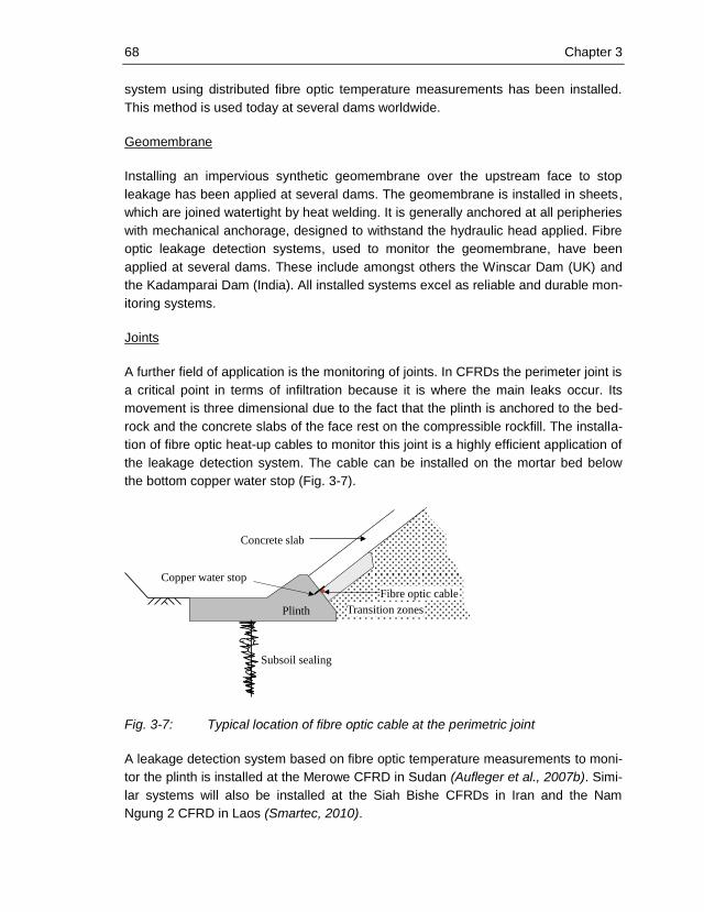
68 Chapter 3
system using distributed fibre optic temperature measurements has been installed.
This method is used today at several dams worldwide.
Geomembrane
Installing an impervious synthetic geomembrane over the upstream face to stop
leakage has been applied at several dams. The geomembrane is installed in sheets,
which are joined watertight by heat welding. It is generally anchored at all peripheries
with mechanical anchorage, designed to withstand the hydraulic head applied. Fibre
optic leakage detection systems, used to monitor the geomembrane, have been
applied at several dams. These include amongst others the Winscar Dam (UK) and
the Kadamparai Dam (India). All installed systems excel as reliable and durable mon-
itoring systems.
Joints
A further field of application is the monitoring of joints. In CFRDs the perimeter joint is
a critical point in terms of infiltration because it is where the main leaks occur. Its
movement is three dimensional due to the fact that the plinth is anchored to the bed-
rock and the concrete slabs of the face rest on the compressible rockfill. The installa-
tion of fibre optic heat-up cables to monitor this joint is a highly efficient application of
the leakage detection system. The cable can be installed on the mortar bed below
the bottom copper water stop (Fig. 3-7).
Fig. 3-7: Typical location of fibre optic cable at the perimetric joint
A leakage detection system based on fibre optic temperature measurements to moni-
tor the plinth is installed at the Merowe CFRD in Sudan (Aufleger et al., 2007b). Simi-
lar systems will also be installed at the Siah Bishe CFRDs in Iran and the Nam
Ngung 2 CFRD in Laos (Smartec, 2010).
Plinth
Concrete slab
Copper water stop
Plinth
Fibre optic cable
Transition zones
Subsoil sealing

Chapter 3 69
Downstream dam toe
The examples listed so far only include applications where a comprehensive rehabili-
tation of the sealing element took place or a new dam was constructed. However, the
monitoring method can also be used for existing dams without any rehabilitation
works. By placing the fibre optic cable in a drainage ditch or below a toe berm the
rising of the phreatic line in the case of seepage can be monitored. Amongst others,
this type of installation was used for the upper reservoir of the pumped storage
scheme Hohenwarte II in Germany, the channel embankments of the hydropower
plants Gabersdorf and St. Dionysen in Austria and the Canal D’Oraison in France.
3.4 Distributed fibre optic strain measurements
3.4.1 General
There is growing interest to measure strain in many engineering structures, such as
dams, bridges and tunnels (Johansson and Watley, 2007). Distributed temperature
and strain sensing (DTSS) allows monitoring of movements along the entire length of
a fibre optic cable. The location as well as the strain in the fibre can be detected,
while in most cases the direction of movement will be unknown. In the following, the
measuring principle and possible applications are briefly introduced. A more detailed
discussion of the monitoring method and application in dams can be found in Jo-
hansson and Watley (2007) and in Hoepffner (2008).
3.4.2 Measuring principle
Regarding the environmental conditions for distributed fibre optic strain sensing in
embankment dams, distributed sensing technologies based on spontaneous light
backscattering are recommended so that measurements can still be performed in the
case of optical fibre breaks up to the location of damage. Commercially available
Brillouin Optical Time Domain Reflectometer (BOTDR) systems allow for distributed
strain and temperature sensing in standard single mode fibres using single end
measurements. The measuring principle of distributed fibre optic strain sensing is
based on the fact that, after sending a light pulse by a powerful light source (laser)
into a glass fibre, a very small proportion of this light is backscattered at each point
along the fibre. Unlike incident light, this scattered light undergoes a shift in frequen-
cy, which is called Brillouin frequency shift and denoted B. The BOTDR unit
measures this frequency, which is assumed to be proportional to temperature varia-
tions and strain. The relation between strain and temperature is given by the follow-
ing equation (Parker et al., 1997)
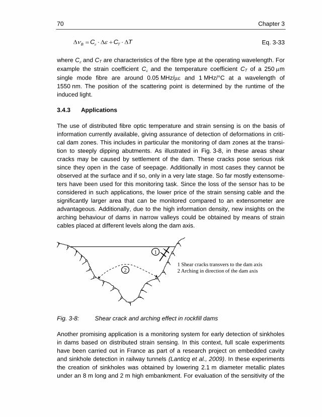
70 Chapter 3
TCC TB Eq. 3-33
where C and CT are characteristics of the fibre type at the operating wavelength. For
example the strain coefficient C and the temperature coefficient CT of a 250 m
single mode fibre are around 0.05 MHz/ and 1 MHz/°C at a wavelength of
1550 nm. The position of the scattering point is determined by the runtime of the
induced light.
3.4.3 Applications
The use of distributed fibre optic temperature and strain sensing is on the basis of
information currently available, giving assurance of detection of deformations in criti-
cal dam zones. This includes in particular the monitoring of dam zones at the transi-
tion to steeply dipping abutments. As illustrated in Fig. 3-8, in these areas shear
cracks may be caused by settlement of the dam. These cracks pose serious risk
since they open in the case of seepage. Additionally in most cases they cannot be
observed at the surface and if so, only in a very late stage. So far mostly extensome-
ters have been used for this monitoring task. Since the loss of the sensor has to be
considered in such applications, the lower price of the strain sensing cable and the
significantly larger area that can be monitored compared to an extensometer are
advantageous. Additionally, due to the high information density, new insights on the
arching behaviour of dams in narrow valleys could be obtained by means of strain
cables placed at different levels along the dam axis.
Fig. 3-8: Shear crack and arching effect in rockfill dams
Another promising application is a monitoring system for early detection of sinkholes
in dams based on distributed strain sensing. In this context, full scale experiments
have been carried out in France as part of a research project on embedded cavity
and sinkhole detection in railway tunnels (Lanticq et al., 2009). In these experiments
the creation of sinkholes was obtained by lowering 2.1 m diameter metallic plates
under an 8 m long and 2 m high embankment. For evaluation of the sensitivity of the
1
21 Shear cracks transvers to the dam axis
2 Arching in direction of the dam axis

Chapter 3 71
monitoring system, the strain sensing cable was installed at two different levels below
the surface. At each level three lines of strain sensing cable were placed. The results
show that deformations in the embankment caused by lowering the metallic plates
more than 35 mm can be detected if the offset of the cable is less than 2.0 m.

72 Chapter 3
Chapter 4 73
4 Laboratory tests
4.1 General
The laboratory tests for distributed fibre optic temperature measurements should
contribute to the further development and improvement of leakage detection and
distributed filter velocity measurement with respect to their application at embank-
ment dams. Based on the findings of the laboratory tests to determine the influence
of mechanical stress on the measurement data, specifications concerning the instal-
lation conditions can be made. The tests on different cables and soils are used to
expand the existing data. These data form an important basis for the specification of
the cable to be installed and the interpretation of in-situ measurements.
With regard to the possible application of distributed fibre optic strain sensing as a
complementary method for monitoring of embankment dams, the goal of the per-
formed laboratory tests is to make statements about the measuring range, the accu-
racy and the repeatability of this measuring method.
In the following, the laboratory tests carried out are described in detail.
4.2 Laboratory tests for distributed filter velocity measurements
4.2.1 General
The distributed filter velocity measurement in granular soils is based on the relation-
ship between heat-transfer coefficient and filter velocity, which is typical for forced
convection. This dependency significantly affects the measured increase in tempera-
ture of a heated cable for filter velocities greater than 10-5
m/s. Distributed filter veloc-
ity measurements demand the knowledge of the influence of the used cable and the
surrounding soil on the correlation between measured temperature differences and
filter velocity. For each cable type this correlation between the temperature difference
and the filter velocity has to be established by laboratory tests. Based on the results
of the laboratory tests calibration curves for the cable for different heat inputs can be
generated.
The aim of the laboratory tests for distributed filter velocity measurements is the
systematic investigation of different soils, commonly used for filters in embankment
dams and different heat up cables.
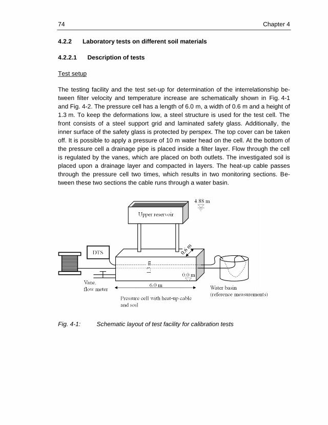
74 Chapter 4
4.2.2 Laboratory tests on different soil materials
4.2.2.1 Description of tests
Test setup
The testing facility and the test set-up for determination of the interrelationship be-
tween filter velocity and temperature increase are schematically shown in Fig. 4-1
and Fig. 4-2. The pressure cell has a length of 6.0 m, a width of 0.6 m and a height of
1.3 m. To keep the deformations low, a steel structure is used for the test cell. The
front consists of a steel support grid and laminated safety glass. Additionally, the
inner surface of the safety glass is protected by perspex. The top cover can be taken
off. It is possible to apply a pressure of 10 m water head on the cell. At the bottom of
the pressure cell a drainage pipe is placed inside a filter layer. Flow through the cell
is regulated by the vanes, which are placed on both outlets. The investigated soil is
placed upon a drainage layer and compacted in layers. The heat-up cable passes
through the pressure cell two times, which results in two monitoring sections. Be-
tween these two sections the cable runs through a water basin.
Fig. 4-1: Schematic layout of test facility for calibration tests
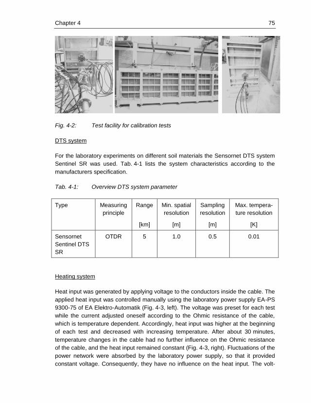
Chapter 4 75
Fig. 4-2: Test facility for calibration tests
DTS system
For the laboratory experiments on different soil materials the Sensornet DTS system
Sentinel SR was used. Tab. 4-1 lists the system characteristics according to the
manufacturers specification.
Tab. 4-1: Overview DTS system parameter
Type Measuring
principle
Range Min. spatial
resolution
Sampling
resolution
Max. tempera-
ture resolution
[km] [m] [m] [K]
Sensornet
Sentinel DTS
SR
OTDR 5 1.0 0.5 0.01
Heating system
Heat input was generated by applying voltage to the conductors inside the cable. The
applied heat input was controlled manually using the laboratory power supply EA-PS
9300-75 of EA Elektro-Automatik (Fig. 4-3, left). The voltage was preset for each test
while the current adjusted oneself according to the Ohmic resistance of the cable,
which is temperature dependent. Accordingly, heat input was higher at the beginning
of each test and decreased with increasing temperature. After about 30 minutes,
temperature changes in the cable had no further influence on the Ohmic resistance
of the cable, and the heat input remained constant (Fig. 4-3, right). Fluctuations of the
power network were absorbed by the laboratory power supply, so that it provided
constant voltage. Consequently, they have no influence on the heat input. The volt-

76 Chapter 4
age and current were recorded continuously during the tests. The heating system is
equipped with an extensive analogue interface for the external setting and monitoring
of the operating parameters voltage and current. The analogue interface suits per-
fectly for the connection of the USB-to-Analog adaptor EA-UTA 12 which enables the
device to be controlled by a PC and allows readout of the relevant data.
Fig. 4-3: Heating system
Conventional temperature measurements
Apart from distributed fibre optic temperature sensing inside the heat-up cables,
conventional temperature probes were used. Temperature was monitored and rec-
orded throughout the test duration inside the pressure cell, inside the water basin and
in the outflow channel (see Fig. 4-4). With the help of conventional temperature
measurements it was tested whether the initial temperature distribution inside the
pressure cell was homogenous and whether the temperature of the percolating water
remained constant during the test. For experiments which did not fully follow these
requirements the temperature recordings could be used for later correction of the test
results. Temperature accuracy of distributed temperature sensing was evaluated with
conventional temperature measurements inside the water basin.

Chapter 4 77
Fig. 4-4: Schematically layout of temperature probes (PT 100) and pressure
transducer
Measurement of pressure decrease in soil
To measure the pressure decrease in the soil layer, two pressure transducers were
installed at the upper and lower layer boundary in the central section of the pressure
cell. The pressure transducers are monitored continuously during the test and data
are logged automatically.
Measurement of flow
The flow rate was regulated manually with the vanes at the outlets. Generally the
vane at the left side of the pressure cell was used. Only for low filter velocities
(wf ≤ 10−5
m/s), which required fine adjustment of the flow rate, the small vane at the
right outflow was used. Discharges smaller than 0.1 l/s were measured using a
measuring cylinder and a stopwatch. Discharges larger than 0.1 l/s were measured
with a hook gauge and a Thomson weir. For discharges larger than 0.3 l/s the flow
rate was recorded automatically by a magnetic inductive flow meter.
Test procedure
A test run for the analysis of the interrelationship between filter velocity and tempera-
ture difference for a specific cable or a specific soil consists of several single tests at
different filter velocities with the same test procedure.
Before starting the experiment a stationary filter velocity inside the pressure cell was
pre-set using the vane at the outflow. The filter velocity was monitored and recorded
over the whole testing time using the flow meter or the Thomson weir. Starting point
of each experiment was a stationary temperature distribution in the pressure cell.
PT 100
water basin
PT 100 soil
(T3, T4)
PT 100 soil
(T1, T2)
Pressure transducer
(P1, P2)
PT 100
outflow channel
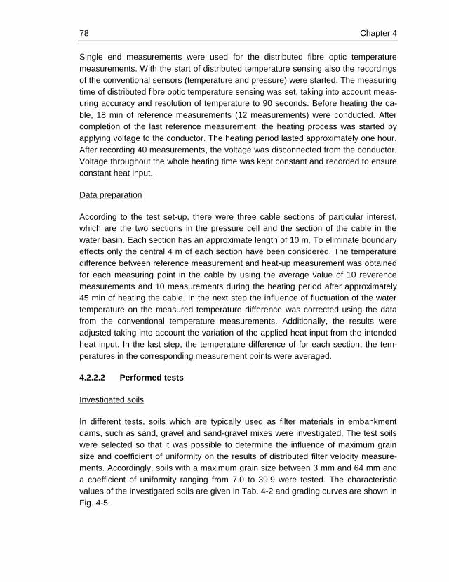
78 Chapter 4
Single end measurements were used for the distributed fibre optic temperature
measurements. With the start of distributed temperature sensing also the recordings
of the conventional sensors (temperature and pressure) were started. The measuring
time of distributed fibre optic temperature sensing was set, taking into account meas-
uring accuracy and resolution of temperature to 90 seconds. Before heating the ca-
ble, 18 min of reference measurements (12 measurements) were conducted. After
completion of the last reference measurement, the heating process was started by
applying voltage to the conductor. The heating period lasted approximately one hour.
After recording 40 measurements, the voltage was disconnected from the conductor.
Voltage throughout the whole heating time was kept constant and recorded to ensure
constant heat input.
Data preparation
According to the test set-up, there were three cable sections of particular interest,
which are the two sections in the pressure cell and the section of the cable in the
water basin. Each section has an approximate length of 10 m. To eliminate boundary
effects only the central 4 m of each section have been considered. The temperature
difference between reference measurement and heat-up measurement was obtained
for each measuring point in the cable by using the average value of 10 reverence
measurements and 10 measurements during the heating period after approximately
45 min of heating the cable. In the next step the influence of fluctuation of the water
temperature on the measured temperature difference was corrected using the data
from the conventional temperature measurements. Additionally, the results were
adjusted taking into account the variation of the applied heat input from the intended
heat input. In the last step, the temperature difference of for each section, the tem-
peratures in the corresponding measurement points were averaged.
4.2.2.2 Performed tests
Investigated soils
In different tests, soils which are typically used as filter materials in embankment
dams, such as sand, gravel and sand-gravel mixes were investigated. The test soils
were selected so that it was possible to determine the influence of maximum grain
size and coefficient of uniformity on the results of distributed filter velocity measure-
ments. Accordingly, soils with a maximum grain size between 3 mm and 64 mm and
a coefficient of uniformity ranging from 7.0 to 39.9 were tested. The characteristic
values of the investigated soils are given in Tab. 4-2 and grading curves are shown in
Fig. 4-5.

Chapter 4 79
Tab. 4-2: Characteristic values of the tested soils
Soil Cl d0-d100 Shape d15 deff Cu
[mm] [mm] [mm] [-]
Sand 0/3 S 0-3 Round 0.13 0.07 7.0
Gravel 0/16 G8 0-16 Round 0.4 0.86 15.8
Gravel 0/32 G9 0-32 Round 0.5 0.96 18.0
Gravel 0/64 G10 0-64 Round 0.5 1.11 39.9
Fig. 4-5: Grading curves of the tested soils
Heat-up cable
The used heat-up cable is shown in Fig. 4-6. The cable is a standard outdoor fibre
optic hybrid cable manufactured by Leoni. It has a central supporting element, six
copper wires with a total cross section of 6 mm2 and a loose tube containing four
G50/125 multimode fibres. The outer jacket consists of HDPE. Its external diameter
is 12.9 mm.
0
10
20
30
40
50
60
70
80
90
100
0.0
1
0.1
0
1.0
0
10
.00
10
0.0
0
10
00
.00
Per
cen
t p
assi
ng
by
wei
gh
t [%
]
Particle size [mm]
S (0/3)
G8 (0/16)
G9 (0/32)
G10 (0/64)
Silt Sand Gravel Cobbles
fine medium coarsefine medium coarsemedium coarse
Boulders

80 Chapter 4
Fig. 4-6: Standard heat-up cable
Artificial cable surrounding
Previous research has shown that the use of artificial cable surroundings may in-
crease the span of temperature difference (Perzlmaier, 2007). Therefore a geotextile
fleece was wrapped around one section of the heat-up cable in the pressure cell to
investigate the influence on the measuring results. The thermophysical properties of
the used material are given in Tab. 4-3 and the arrangement of the geotextile fleece
is shown in Fig. 4-7.
Tab. 4-3: Characteristic values of artificial cable surrounding
Geotextile
Naue
Secutex®
PP coloured
Geometric Thermal
Thick
ness
[mm]
msp
[g/m2]
s,exp
[t/m3
]
d,exp
[t/m3]
n
[%]
kf,cal
[m/s]
cp
[m/s]
eff,exp
[W/(m K)]
Fleec
e
Fr 5.4 800 0.83 0.14 83.0 3.5∙10-2
1170 0.51
No. Manu-
facturer
Diam.
[mm]
No. of
conductors
Material Cross section
[mm2]
No. of
fibres
Remark
1 Leoni 12.9 6 CU 6 x 1.5 4 Strength member
Central strength member
Loose tube
Water absorbent tape
Cu wire
Rip cord
Armour
HDPE outer jacket
Cable 1

Chapter 4 81
Fig. 4-7: Artificial cable surrounding
Test series
The laboratory tests to investigate the influence of soil on the results of distributed
filter velocity measurements comprise four tests series. Tab. 4-4 summarizes the
performed test series.
Tab. 4-4: Overview of tests for investigation of influence of soil material
Year Series Cable
No. / Di
am.
Soil Cable
surround-
ing
DTS
system
Heat
input
Direction of
flow
[mm] [W/m]
2009 S-1 A 1/12.9 S --- Sensornet 12 downward
B 1/12.9 S Fr Sensornet 12 downward
2010 S-2 A 1/12.9 G8 --- Sensornet 12 downward
B 1/12.9 G8 Fr Sensornet 12 downward
S-3 A 1/12.9 G9 Sensornet 12 downward
B 1/12.9 G9 Fr Sensornet 12 downward
S-4 A 1/12.9 G10 --- Sensornet 12 downward
B 1/12.9 G10 Fr Sensornet 12 downward
Results
The results of the tests are pairs of values of pre-set filter velocity and measured
temperature difference. The measuring data are processed according to the proce-
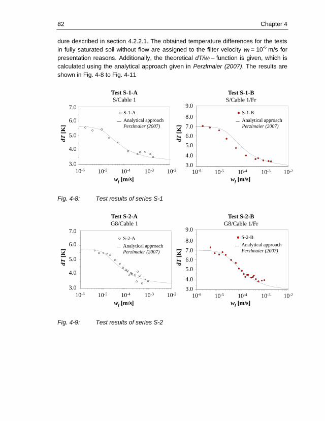
82 Chapter 4
dure described in section 4.2.2.1. The obtained temperature differences for the tests
in fully saturated soil without flow are assigned to the filter velocity wf = 10-6
m/s for
presentation reasons. Additionally, the theoretical dT/wf – function is given, which is
calculated using the analytical approach given in Perzlmaier (2007). The results are
shown in Fig. 4-8 to Fig. 4-11
Fig. 4-8: Test results of series S-1
Fig. 4-9: Test results of series S-2
3.0
4.0
5.0
6.0
7.0
8.0
9.0
1E-6 1E-5 1E-4 1E-3 1E-2
23A
7.0
6.0
5.0
4.0
3.0
10-6 10-5 10-4 10-3 10-2
Test S-1-A
S/Cable 1
8.0
7.0
5.0
4.0
10-6 10-5 10-4 10-3 10-2
6.0
9.0
3.0
Test S-1-B
S/Cable 1/Fr
dT
[K]
dT
[K]
wf [m/s] wf [m/s]
3.0
4.0
5.0
6.0
7.0
1E-6 1E-5 1E-4 1E-3 1E-2
23AS-1-A
Analytical approach
Perzlmaier (2007)
S-1-B
Analytical approach
Perzlmaier (2007)
7.0
6.0
5.0
4.0
3.0
10-6 10-5 10-4 10-3 10-2
Test S-2-A
G8/Cable 1
8.0
7.0
5.0
4.0
10-6 10-5 10-4 10-3 10-2
6.0
9.0
3.0
Test S-2-B
G8/Cable 1/Fr
dT
[K]
dT
[K]
wf [m/s] wf [m/s]
3.0
4.0
5.0
6.0
7.0
1E-6 1E-5 1E-4 1E-3 1E-2
25AS-2-A
Analytical approach
Perzlmaier (2007)
3.0
4.0
5.0
6.0
7.0
8.0
9.0
1E-6 1E-5 1E-4 1E-3 1E-2
25BS-2-B
Analytical approach
Perzlmaier (2007)
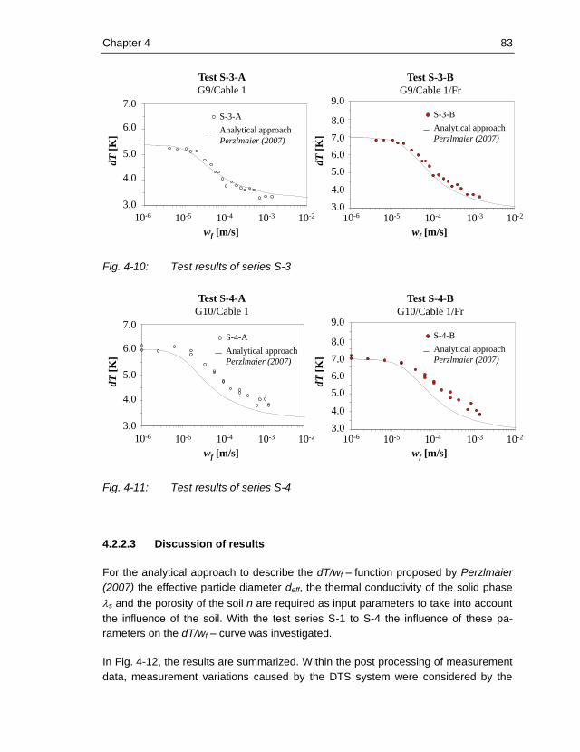
Chapter 4 83
Fig. 4-10: Test results of series S-3
Fig. 4-11: Test results of series S-4
4.2.2.3 Discussion of results
For the analytical approach to describe the dT/wf – function proposed by Perzlmaier
(2007) the effective particle diameter deff, the thermal conductivity of the solid phase
s and the porosity of the soil n are required as input parameters to take into account
the influence of the soil. With the test series S-1 to S-4 the influence of these pa-
rameters on the dT/wf – curve was investigated.
In Fig. 4-12, the results are summarized. Within the post processing of measurement
data, measurement variations caused by the DTS system were considered by the
7.0
6.0
5.0
4.0
3.0
10-6 10-5 10-4 10-3 10-2
Test S-3-A
G9/Cable 1
8.0
7.0
5.0
4.0
10-6 10-5 10-4 10-3 10-2
6.0
9.0
3.0
Test S-3-B
G9/Cable 1/Fr
dT
[K]
dT
[K]
wf [m/s] wf [m/s]
3.0
4.0
5.0
6.0
7.0
1E-6 1E-5 1E-4 1E-3 1E-2
26AS-3-A
Analytical approach
Perzlmaier (2007)
3.0
4.0
5.0
6.0
7.0
8.0
9.0
1E-6 1E-5 1E-4 1E-3 1E-2
26BS-3-B
Analytical approach
Perzlmaier (2007)
7.0
6.0
5.0
4.0
3.0
10-6 10-5 10-4 10-3 10-2
Test S-4-A
G10/Cable 1
8.0
7.0
5.0
4.0
10-6 10-5 10-4 10-3 10-2
6.0
9.0
3.0
Test S-4-B
G10/Cable 1/Frd
T[K
]
dT
[K]
wf [m/s] wf [m/s]
3.0
4.0
5.0
6.0
7.0
1E-6 1E-5 1E-4 1E-3 1E-2
27AS-4-A
Analytical approach
Perzlmaier (2007)
3.0
4.0
5.0
6.0
7.0
8.0
9.0
1E-6 1E-5 1E-4 1E-3 1E-2
27BS-4-B
Analytical approach
Perzlmaier (2007)
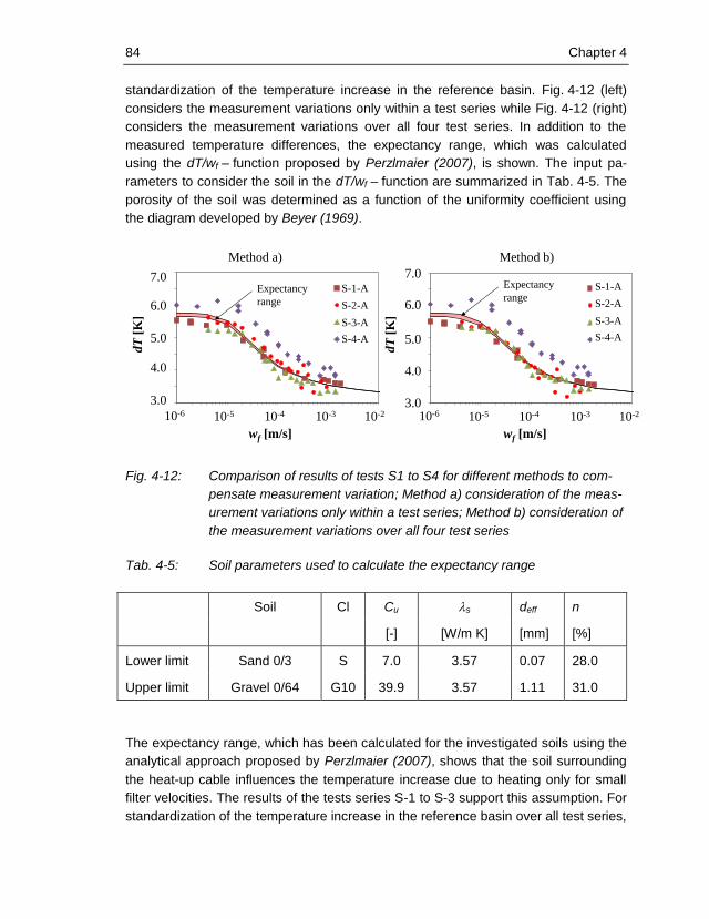
84 Chapter 4
standardization of the temperature increase in the reference basin. Fig. 4-12 (left)
considers the measurement variations only within a test series while Fig. 4-12 (right)
considers the measurement variations over all four test series. In addition to the
measured temperature differences, the expectancy range, which was calculated
using the dT/wf – function proposed by Perzlmaier (2007), is shown. The input pa-
rameters to consider the soil in the dT/wf – function are summarized in Tab. 4-5. The
porosity of the soil was determined as a function of the uniformity coefficient using
the diagram developed by Beyer (1969).
Fig. 4-12: Comparison of results of tests S1 to S4 for different methods to com-
pensate measurement variation; Method a) consideration of the meas-
urement variations only within a test series; Method b) consideration of
the measurement variations over all four test series
Tab. 4-5: Soil parameters used to calculate the expectancy range
Soil Cl Cu s deff n
[-] [W/m K] [mm] [%]
Lower limit Sand 0/3 S 7.0 3.57 0.07 28.0
Upper limit Gravel 0/64 G10 39.9 3.57 1.11 31.0
The expectancy range, which has been calculated for the investigated soils using the
analytical approach proposed by Perzlmaier (2007), shows that the soil surrounding
the heat-up cable influences the temperature increase due to heating only for small
filter velocities. The results of the tests series S-1 to S-3 support this assumption. For
standardization of the temperature increase in the reference basin over all test series,
3,0
4,0
5,0
6,0
7,0
1,E-06 1,E-05 1,E-04 1,E-03 1,E-02
K4
B1
B2
B3
3,0
4,0
5,0
6,0
7,0
1,E-06 1,E-05 1,E-04 1,E-03 1,E-02
K4
B1
B2
B3
7.0
6.0
5.0
4.0
3.0
10-6 10-5 10-4 10-3 10-2
7.0
5.0
4.0
10-6 10-5 10-4 10-3 10-2
6.0
3.0d
T[K
]
dT
[K]
wf [m/s] wf [m/s]
S-1-A
S-2-A
S-3-A
S-4-A
S-1-A
S-2-A
S-3-A
S-4-A
Expectancy
range
Expectancy
range
Method a) Method b)

Chapter 4 85
no dependence between the measured temperature difference and the used soil
materials S-1, S-2 and S-3 is apparent (Fig. 4-12, right). It is remarkable that the
temperature differences measured for test series S-4 are much higher than in the
previous experiments. The measurement data suggest an increased heat input. Tak-
ing into account the linear relationship between heat input and increase in tempera-
ture, the heat input would have been 15% higher than in the other test series. How-
ever, both the measured temperature differences in the reference basin (Fig. 4-13)
and the recorded data of the heating system contradict this assumption.
Fig. 4-13: Temperature differences obtained from the reference basin for test
series S-1 to S-4
Another explanation for this phenomenon could be that the flow velocity in the imme-
diate vicinity of the cable is lower than the average filter velocity determined from the
outflow. Unlike the other tested materials, the sand-gravel mixture G10 segregated
during placement resulting in honeycombs, lower degree of compaction and high
permeable zones, especially along the boundaries (Fig. 4-14). Accordingly, it can be
assumed that the flow through the soil takes places through the higher permeable
zones and the determined filter velocity is not representative for the flow in the imme-
diate vicinity of the cable. Fig. 4-6 shows the modified results, assuming that the filter
velocity along the cable is only about 25% of the average filter velocity.
4,00
4,20
4,40
4,60
4,80
5,00
5,20
5,40
5,60
5,80
6,00
0 10 20 30 40 50 60 70 80
Mittelwert
K4
B1
B2
B3
4.0
4.4
5.2
4.8
5.6
6.0
dT
[K]
0 10 20 30 40 50 60 70 80
Test No.
S-1 S-2 S-3 B2S-4

86 Chapter 4
Fig. 4-14: Honeycombs due to segregation of G10 material
Fig. 4-15: Comparison of results with adjusted filter velocity wf for test series S-4
However, this would not explain the three outliers for filter velocities between wf = 10-
6 m/s and 10
-5 m/s. It is anticipated that the compactness of the soil has a larger influ-
ence on the increase of temperature due to heating than previously thought. There-
fore, in the next phases of research additional laboratory tests to investigate the
influence of the compactness of the soil will be carried out.
4.2.3 Laboratory tests for optimized heat-up cables
4.2.3.1 Description of tests
Part of the experiments to study different heat-up cables was carried out within the
framework of a research project funded by the Bayrische Forschungsstiftung (BFS) at
the hydraulic laboratory of the TU München using the existent testing facility with the
associated measuring equipment. It is described in detail in (Perzlmaier, 2007). How-
3,0
4,0
5,0
6,0
7,0
1,E-06 1,E-05 1,E-04 1,E-03 1,E-02
K4
B1
B2
B3
7.0
6.0
5.0
4.0
3.010-6 10-5 10-4 10-3 10-2
dT
[K]
wf [m/s]
S-1-A
S-2-A
S-3-A
S-4-A
Outliers

Chapter 4 87
ever, the testing facility, measuring equipment and test procedure comply with the
description given in section 4.2.2.1, so that the continuity of the test series is en-
sured.
4.2.3.2 Performed tests
Heat-up cables
In the course of the laboratory tests for optimized heat-up cables, the hybrid cables
shown in Fig. 4-16 were investigated. Cable 2 is a standard outdoor fibre optic hybrid
cable manufactured by Helu Kabel. The main field of application of the cable is leak-
age detection in hydraulic engineering structures. It has a central supporting element,
four copper conductors with a total cross-section of 6 mm2 and a loose tube contain-
ing four G50/125 multimode fibres. The coating consists of PE. The external diameter
is 17.0 mm.
Cable 3 to cable 5 are optimized heat-up cables which were developed within the
framework of a research project funded by the Bayrische Forschungsstiftung (BFS).
Perzlmaier (2007) concluded based on his research findings that a reduction of the
outer diameter of the heat-up cable contributes to an increase of measuring accuracy
of distributed filter velocity measurements. Therefore, the optimization of the cables
was based on the principle of minimizing all cable components except for the electri-
cal conductors. In the design of the cables, both metrological requirements and the
demand on an economical production process have been considered. The configura-
tion of the cable has been adjusted with the cable manufacturer Leoni Fibre Optics
GmbH in such a way that the production of the cables can take place on conventional
production lines with a reasonable expenditure of time and costs. The design of ca-
ble 3 is based on the configuration of a conventional hybrid cable. A reduction of
diameter to 8.4 mm was achieved by omitting the strength member and minimization
of the outer jacket. The reduction of conductor cross section to 3 mm2 only has ad-
verse effects for long cable lengths. In cable 4 the wires are placed without insulation
by which a very thin hybrid cable is obtained. However this cable can only be used,
where the cable can be placed in an external loop since both cable ends have to be
connected to the power source. Cable 5 has a diameter similar to that of cable 3 but
allows for significantly longer sections to be monitored due to the large conductor
cross section. All optimized cables use the thinner and more robust HDPE coatings
instead of PE coatings.

88 Chapter 4
Fig. 4-16: Design of tested heat-up cables
Soil material and artificial cable surroundings
For the laboratory tests on optimized heat-up cables, the well-graded sand with parti-
cle sizes of 0 to 3 mm was used. The characteristic parameters and the grading
curve of the sand are given in Tab. 4-2 and Fig. 4-5. The fleece used as artificial
cable surrounding is shown in Fig. 4-7.
Test series
The laboratory tests for optimized heat-up cables comprise four test series. Tab. 4-4
summarizes the performed test series. Additionally, the results of test series S-1 (see
Fig. 4-8, section 4.2.2.2) are taken into account for the evaluation of the influence of
the cable.
Cable 2
No. Manu-
facturer
Diam.
[mm]
No. of
conductors
Material Cross section
[mm2]
No. of
fibres
Remark
2 Helu-
Kabel
17.0 4 CU 4 x 1.5 4 Strength
member
3 Leoni 8.4 6 CU 6 x 0.5 4 ---
4 Leoni 5.6 Stranded wires CU 4.0 4 External loop
5 Leoni 8.3 Stranded wires CU 2 x 4.0 4
Loose tube
Cable 3
Cu wire
Rip cord
HDPE
outer jacket
Loose tube
HDPE
outer jacket
Cu wireLoose tube
Cu wire
HDPE inner jacket
HDPE
outer jacket
Shield
Cable 4 Cable 5
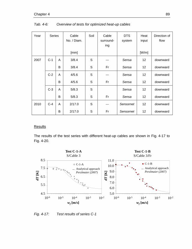
Chapter 4 89
Tab. 4-6: Overview of tests for optimized heat-up cables
Year Series Cable
No. / Diam.
Soil Cable
surround-
ing
DTS
system
Heat
input
Direction of
flow
[mm] [W/m]
2007 C-1 A 3/8.4 S --- Sensa 12 downward
B 3/8.4 S Fr Sensa 12 downward
C-2 A 4/5.6 S --- Sensa 12 downward
B 4/5.6 S Fr Sensa 12 downward
C-3 A 5/8.3 S Sensa 12 downward
B 5/8.3 S Fr Sensa 12 downward
2010 C-4 A 2/17.0 S --- Sensornet 12 downward
B 2/17.0 S Fr Sensornet 12 downward
Results
The results of the test series with different heat-up cables are shown in Fig. 4-17 to
Fig. 4-20.
Fig. 4-17: Test results of series C-1
8.5
7.5
6.5
5.5
4.5
10-6 10-5 10-4 10-3 10-2
C-1-A
Test C-1-A
S/Cable 3
11.0
9.0
8.0
6.0
5.0
10-6 10-5 10-4 10-3 10-2
7.0
10.0
Test C-1-B
S/Cable 3/Fr
dT
[K]
dT
[K]
wf [m/s] wf [m/s]
4.5
5.5
6.5
7.5
8.5
1E-6 1E-5 1E-4 1E-3 1E-2
18A
C-1-A
Analytical approach
Perzlmaier (2007)
5.0
6.0
7.0
8.0
9.0
10.0
11.0
1E-6 1E-5 1E-4 1E-3 1E-2
18BC-1-B
Analytical approach
Perzlmaier (2007)
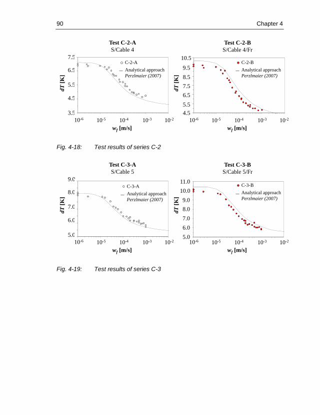
90 Chapter 4
Fig. 4-18: Test results of series C-2
Fig. 4-19: Test results of series C-3
7.5
6.5
5.5
4.5
3.5
10-6 10-5 10-4 10-3 10-2
Test C-2-A
S/Cable 4
10.5
8.5
7.5
5.5
4.5
10-6 10-5 10-4 10-3 10-2
6.5
9.5
Test C-2-B
S/Cable 4/Fr
dT
[K]
dT
[K]
wf [m/s] wf [m/s]
3.5
4.5
5.5
6.5
7.5
1E-6 1E-5 1E-4 1E-3 1E-2
19A
4.5
5.5
6.5
7.5
8.5
9.5
10.5
1E-6 1E-5 1E-4 1E-3 1E-2
19B
C-2-B
Analytical approach
Perzlmaier (2007)
C-2-A
Analytical approach
Perzlmaier (2007)
5.0
6.0
7.0
8.0
9.0
10.0
11.0
1E-6 1E-5 1E-4 1E-3 1E-2
20B
9.0
8.0
7.0
6.0
5.0
10-6 10-5 10-4 10-3 10-2
Test C-3-A
S/Cable 5
10.0
8.0
7.0
11.0
10-5 10-4 10-3 10-2
6.0
9.0
5.010-6
Test C-3-B
S/Cable 5/Frd
T[K
]
dT
[K]
wf [m/s] wf [m/s]
5.0
6.0
7.0
8.0
9.0
1E-6 1E-5 1E-4 1E-3 1E-2
20A
C-3-A
Analytical approach
Perzlmaier (2007)
C-3-B
Analytical approach
Perzlmaier (2007)

Chapter 4 91
Fig. 4-20: Test results of series C-4
4.2.3.3 Discussion of results
For small flow or no flow around the cable, the temperature rise due to heating in-
creases with decreasing cable diameter. The reason is that with decreasing cable
diameter, the surface area available for conductive heat transfer, which is dominant
for these flow regimes, decreases. For large flow around the cable, heat transfer is
dominated by forced convection. In this case the amount of heat transported away
depends mostly on the flow velocity of the fluid and the influence of the surface area
available for heat transfer diminishes. Consequently, the span of measured tempera-
ture differences increases with decreasing cable diameter (Perzlmaier, 2007). As
shown in Fig. 4-21, the obtained results clearly demonstrate this relationship. The
effect can be amplified by using artificial cable surroundings with low thermal conduc-
tivity and permeability similar to the surrounding soil.
7.5
6.5
5.5
4.5
3.5
10-6 10-5 10-4 10-3 10-2
Test C-4-A
S/Cable 2
9.0
8.0
6.0
5.0
10-5 10-4 10-3 10-2
7.0
10.0
4.010-6
Test C-4-B
S/Cable 2/Fr
dT
[K]
dT
[K]
wf [m/s] wf [m/s]
3.5
4.5
5.5
6.5
7.5
1E-6 1E-5 1E-4 1E-3 1E-2
24A
4.0
5.0
6.0
7.0
8.0
9.0
10.0
1E-6 1E-5 1E-4 1E-3 1E-2
24BC-4-A
Analytical approach
Perzlmaier (2007)
C-4-B
Analytical approach
Perzlmaier (2007)

92 Chapter 4
Fig. 4-21: Span of temperature differences against cable diameter for tested
cables
Distributed filter velocity measurements require that the span between temperature
differences obtained for small or no flow around the cable and temperature differ-
ences for large flow around the cable is sufficiently large compared to the measure-
ments variations of distributed fibre optic temperature measurements. Therefore, the
different heat-up cables can be assessed using the span of temperature differences
deducted from the laboratory test results. For each tested cable the span of tempera-
ture differences was calculated in accordance to the test results using the approach
proposed by Perzlmaier (2007). The results are summarized in Tab. 4-7.
0
1
2
3
4
5
6
7
8
4 6 8 10 12 14 16 18 204 6 8 10 12 14 16 18 200
1
2
3
4
5
6
7
8
Cable diameter D [mm]
Sp
an o
f te
mp
erat
ure
dT
[K]
With geotextile
Heat input q = 12 W/m,
Heating time 1 h
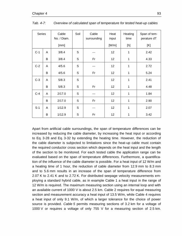
Chapter 4 93
Tab. 4-7: Overview of calculated span of temperature for tested heat-up cables
Series Cable
No. / Diam.
Soil Cable
surrounding
Heat
input
Heating
time
Span of tem-
perature dT
[mm] [W/m] [h] [K]
C-1 A 3/8.4 S --- 12 1 2.42
B 3/8.4 S Fr 12 1 4.33
C-2 A 4/5.6 S --- 12 1 2.72
B 4/5.6 S Fr 12 1 5.24
C-3 A 5/8.3 S 12 1 2.41
B 5/8.3 S Fr 12 1 4.48
C-4 A 2/17.0 S --- 12 1 1.84
B 2/17.0 S Fr 12 1 2.90
S-1 A 1/12.9 S --- 12 1 2.07
B 1/12.9 S Fr 12 1 3.42
Apart from artificial cable surroundings, the span of temperature differences can be
increased by reducing the cable diameter, by increasing the heat input or according
to Eq. 3-28 and Eq. 3-32 by extending the heating time. However, the reduction of
the cable diameter is subjected to limitations since the heat-up cable must contain
the required conductor cross section which depends on the heat input and the length
of the section to be monitored. For each tested cable the application range can be
evaluated based on the span of temperature differences. Furthermore, a quantifica-
tion of the influence of the cable diameter is possible. For a heat input of 12 W/m and
a heating time of 1 hour, the reduction of cable diameter from 12.9 mm to 8.3 mm
and to 5.6 mm results in an increase of the span of temperature difference from
2.07 K to 2.41 K and to 2.72 K. For distributed seepage velocity measurements em-
ploying a standard hybrid cable, as in example Cable 1 a heat input in the range of
12 W/m is required. The maximum measuring section using an internal loop and with
an available current of 1000 V is about 2.5 km. Cable 2 requires for equal measuring
section and measurement accuracy a heat input of 13.5 W/m, while Cable 4 requires
a heat input of only 9.1 W/m, of which a larger tolerance for the choice of power
source is provided. Cable 5 permits measuring sections of 3.2 km for a voltage of
1000 V or requires a voltage of only 755 V for a measuring section of 2.5 km.
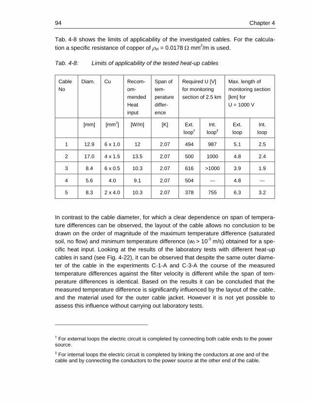
94 Chapter 4
Tab. 4-8 shows the limits of applicability of the investigated cables. For the calcula-
tion a specific resistance of copper of el = 0.0178 mm2/m is used.
Tab. 4-8: Limits of applicability of the tested heat-up cables
Cable
No
Diam. Cu Recom-
om-
mended
Heat
input
Span of
tem-
perature
differ-
ence
Required U [V]
for monitoring
section of 2.5 km
Max. length of
monitoring section
[km] for
U = 1000 V
[mm] [mm2] [W/m] [K] Ext.
loop†
Int.
loop‡
Ext.
loop
Int.
loop
1 12.9 6 x 1.0 12 2.07 494 987 5.1 2.5
2 17.0 4 x 1.5 13.5 2.07 500 1000 4.8 2.4
3 8.4 6 x 0.5 10.3 2.07 616 >1000 3.9 1.9
4 5.6 4.0 9.1 2.07 504 --- 4.8 ---
5 8.3 2 x 4.0 10.3 2.07 378 755 6.3 3.2
In contrast to the cable diameter, for which a clear dependence on span of tempera-
ture differences can be observed, the layout of the cable allows no conclusion to be
drawn on the order of magnitude of the maximum temperature difference (saturated
soil, no flow) and minimum temperature difference (wf > 10-3
m/s) obtained for a spe-
cific heat input. Looking at the results of the laboratory tests with different heat-up
cables in sand (see Fig. 4-22), it can be observed that despite the same outer diame-
ter of the cable in the experiments C-1-A and C-3-A the course of the measured
temperature differences against the filter velocity is different while the span of tem-
perature differences is identical. Based on the results it can be concluded that the
measured temperature difference is significantly influenced by the layout of the cable,
and the material used for the outer cable jacket. However it is not yet possible to
assess this influence without carrying out laboratory tests.
† For external loops the electric circuit is completed by connecting both cable ends to the power
source.
‡ For internal loops the electric circuit is completed by linking the conductors at one and of the
cable and by connecting the conductors to the power source at the other end of the cable.

Chapter 4 95
Fig. 4-22: Comparison of results of tests C-1 to C-4 and S-1
4.3 Laboratory tests to determine influence of mechanical stress
4.3.1 General
In general ordinary fibre optic cables as used for telecommunication purposes are
used for distributed fibre optic temperature measurements. However, the specifica-
tions of these cables, which are based on standardized testing methods, give only
limited information regarding the applicability of the cables for installation in em-
bankment dams. Therefore, the laboratory tests described below were carried out at
the University of Innsbruck. In several test series possible installation conditions and
expected loads due to overburden pressure (pressure perpendicular to the cable
axis) and elongation (tensile forces) were simulated to investigate if they affect the
results of the temperature measurements.
4.3.2 Laboratory test for investigation of influence of pressure perpendicu-
lar to the cable axis
4.3.2.1 Description of tests
Testing Facility
The laboratory tests for determination of the effects of pressure perpendicular to the
cable axis on the results of DFOT measurements were carried out using the testing
facility shown in Fig. 4-23. The cable is installed in a 3.78 m long, 0.6 m wide and 0.6
m high reinforced steel box using different bedding materials. The load was applied
3,0
4,0
5,0
6,0
7,0
8,0
9,0
1E-6 1E-5 1E-4 1E-3 1E-2
18A
19A
20A
24A
23A
3,0
4,0
5,0
6,0
7,0
8,0
9,0
1E-6 1E-5 1E-4 1E-3 1E-2
18A
19A
20A
24A
23A
7.0
6.0
5.0
4.0
3.0
10-6 10-5 10-4 10-3 10-2
8.0
9.0C-1-AC-2-AC-3-AC-4-AS-1-A 8.0
7.0
5.0
4.0
10-6 10-5 10-4 10-3 10-2
6.0
9.0
3.0
10.0
11.0
dT
[K
]
dT
[K]
wf [m/s] wf [m/s]
C-1-BC-2-BC-3-BC-4-BS-1-B
Tests in sand without
artificial cable surrounding
Tests in sand with
artificial cable surrounding
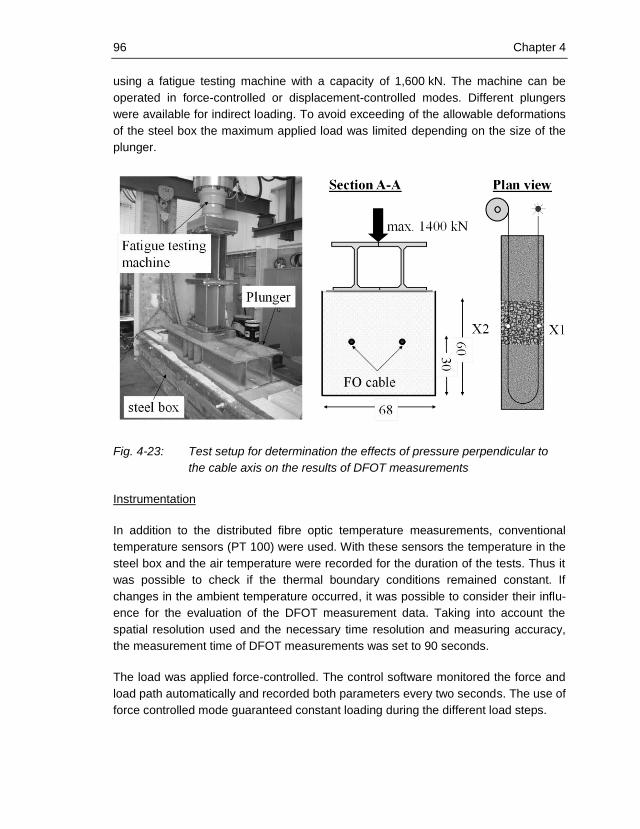
96 Chapter 4
using a fatigue testing machine with a capacity of 1,600 kN. The machine can be
operated in force-controlled or displacement-controlled modes. Different plungers
were available for indirect loading. To avoid exceeding of the allowable deformations
of the steel box the maximum applied load was limited depending on the size of the
plunger.
Fig. 4-23: Test setup for determination the effects of pressure perpendicular to
the cable axis on the results of DFOT measurements
Instrumentation
In addition to the distributed fibre optic temperature measurements, conventional
temperature sensors (PT 100) were used. With these sensors the temperature in the
steel box and the air temperature were recorded for the duration of the tests. Thus it
was possible to check if the thermal boundary conditions remained constant. If
changes in the ambient temperature occurred, it was possible to consider their influ-
ence for the evaluation of the DFOT measurement data. Taking into account the
spatial resolution used and the necessary time resolution and measuring accuracy,
the measurement time of DFOT measurements was set to 90 seconds.
The load was applied force-controlled. The control software monitored the force and
load path automatically and recorded both parameters every two seconds. The use of
force controlled mode guaranteed constant loading during the different load steps.
Chapter 4 97
Test procedure
After installation of the cable in the soil material, it took a certain amount of time until
stationary thermal conditions were reached which were necessary to start the tests.
Before applying the load, reference measurements were conducted for about 10
minutes. The load was applied in load steps of 125 kN. Each load step took 6
minutes. After completion of the final load step the sample was unloaded. For some
tests it was necessary to unload the sample and to place spacers, because the set-
tlements were larger than the maximum cylinder stroke of the testing equipment.
After placing the spacers, the sample was reloaded in steps up to the previous load
stage reached, and then the load was further increased according to the test pro-
gram.
4.3.2.2 Performed tests
Investigated soils
In different tests, soils which are typically used as filter materials in embankment
dams, such as sand, gravel and sand-gravel mixes were investigated. The test soils
were selected so that it was possible to determine the influence of maximum grain
size, coefficient of uniformity and particle shape of the bedding material on the results
of distributed fibre optic temperature measurements. Accordingly, soils with a maxi-
mum grain size between 3 mm and 64 mm, and a coefficient of uniformity ranging
from 1.5 to 32 as well as round (natural) and processed material were tested. The
characteristic values of the soils used as bedding material are given in Tab. 4-9, and
grading curves are shown in Fig. 4-24.

98 Chapter 4
Tab. 4-9: Characteristic values of the soils used as bedding material
Soil Cl d0-d100 Shape d15 deff Cu
[mm] [mm] [mm] [-]
Sand 0/3 S 0-3 Round 0.13 0.07 7.0
Gravel 0/16 G1 0-16 Round 0.36 0.48 13.2
Gravel 0/16 G2 0-16 Processed 0.33 0.45 12.4
Gravel 0/32 G3 0-32 Round 0.64 0.66 30.7
Gravel 0/32 G4 0-32 Processed 0.39 0.32 32.1
Gravel 0/64 G5 0-64 Processed 4.6 2.32 6.0
Gravel 4/8 G6 4-8 Processed 4.6 5.33 1.5
Gravel 8/16 G7 8-16 Round 9.2 10.67 1.5
Fig. 4-24: Grading curves of the soils used as bedding material
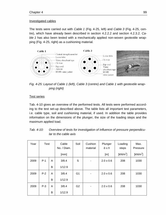
Chapter 4 99
Investigated cables
The tests were carried out with Cable 1 (Fig. 4-25, left) and Cable 3 (Fig. 4-25, cen-
tre), which have already been described in section 4.2.2.2 and section 4.2.3.2. Ca-
ble 1 has also been tested with a mechanically applied non-woven geotextile wrap-
ping (Fig. 4-25, right) as a cushioning material.
Fig. 4-25: Layout of Cable 1 (left), Cable 3 (centre) and Cable 1 with geotextile wrap-
ping (right)
Test series
Tab. 4-10 gives an overview of the performed tests. All tests were performed accord-
ing to the test set-up described above. The table lists all important test parameters,
i.e. cable type, soil and cushioning material, if used. In addition the table provides
information on the dimensions of the plunger, the size of the loading steps and the
maximum applied load.
Tab. 4-10: Overview of tests for investigation of influence of pressure perpendicu-
lar to the cable axis
Year Test Cable
No. / Diam.
Soil Cushion
material
Plunger
b x h
Loading
steps
Max.
Pressure
[mm] [m] [kN/m2] [kN/m
2]
2009 P-1 A 3/8.4 S - 2.0 x 0.6 208 1030
B 1/12.9
2009 P-2 A 3/8.4 G1 - 2.0 x 0.6 208 1030
B 1/12.9
2009 P-3 A 3/8.4 G2 - 2.0 x 0.6 208 1030
B 1/12.9

100 Chapter 4
Year Test Cable
No. / Diam.
Soil Cushion
material
Plunger
b x h
Loading
steps
Max.
Pressure
[mm] [m] [kN/m2] [kN/m
2]
2009 P-4 B 1/12.9 G5 - 2.0 x 0.6 208 4000
2009 P-5 A 3/8.4 G5 - 0.5 x 0.5 500 3000
2009 P-6 A 3/8.4 G5 - 0.5 x 0.5 500 3000
B 1/12.9
C 1/12.9
2009 P-7 A 3/8.4 G2 - 0.5 x 0.5 500 3000
B 1/12.9
2009 P-8 A 3/8.4 G4 - 0.5 x 0.5 500 3000
B 1/12.9
C 1/12.9
2009 P-9 A 3/8.4 G3 - 0.5 x 0.5 500 3000
B 1/12.9
C 1/12.9
2009 P-10 A 3/8.4 G7 - 0.5 x 0.5 500 3000
B 1/12.9
C 1/12.9
2009 P-11 A 3/8.4 G6 - 0.5 x 0.5 500 3000
B 1/12.9
C 1/12.9
Results
The evaluation of the results mainly focused on the measuring points just below the
plunger. Since the DFOT measurement data showed little noise, smoothing of the
data was not necessary. To determine the influence of pressure perpendicular to the

Chapter 4 101
cable axis on the DFOT measurement data, the temperature difference between the
reference temperature measured in the unloaded state and the temperature meas-
ured in the loaded state was calculated and plotted against the applied load. Chang-
es of the thermal boundary conditions during the tests were considered by means of
the temperature data obtained from the conventional temperature sensors.
Fig. 4-26 exemplarily shows the results of the DFOT measurement depending on the
applied load perpendicular to the cable axis. Because of the used bedding material in
test P-7-B, which is a processed sand gravel mix 0/16, the temperature results are
not affected by the applied load. In contrast, the results of the DFOT measurements
for test P-10-B, which uses a uniform natural gravel 8/16, are significantly affected by
the applied load. The results of all tests are presented in 0.
Fig. 4-26: Results of laboratory tests for investigation of influence of pressure
perpendicular to the cable axis
4.3.2.3 Discussion of the results
General
Based on the obtained measurement data, the influence of pressure perpendicular to
the cable axis on the results of distributed fibre optic temperature measurements is
discussed. Primarily the experiments provide knowledge of the maximum admissible
load for a specific cable depending on the bedding material used. Tab. 4-11 lists the
maximum applied loads, which did not distort the measurement data.
Test P-7-B Test P-10-B
Time Time
dT
[ C
]
dT
[ C
]
Com
pre
ssio
n[k
N/m
2]
Com
pre
ssio
n[k
N/m
2]
0
400
800
1200
1600
2000
2400
2800
3200
3600
4000
-28.00
-24.00
-20.00
-16.00
-12.00
-8.00
-4.00
0.00
4.00
8.00
12.00
6:57 7:12 7:26 7:40 7:55 8:09 8:24
dT Point X1dT Point X2Load
0
400
800
1200
1600
2000
2400
2800
3200
3600
4000
-72.00
-64.00
-56.00
-48.00
-40.00
-32.00
-24.00
-16.00
-8.00
0.00
8.00
7:04 7:19 7:33 7:48 8:02 8:16
dT Point X1
dT Point X2
Load
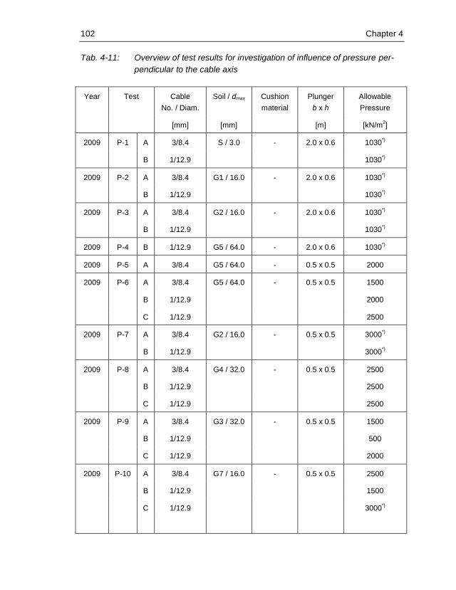
102 Chapter 4
Tab. 4-11: Overview of test results for investigation of influence of pressure per-
pendicular to the cable axis
Year Test Cable
No. / Diam.
Soil / dmax Cushion
material
Plunger
b x h
Allowable
Pressure
[mm] [mm] [m] [kN/m2]
2009 P-1 A 3/8.4 S / 3.0 - 2.0 x 0.6 1030*)
B 1/12.9 1030*)
2009 P-2 A 3/8.4 G1 / 16.0 - 2.0 x 0.6 1030*)
B 1/12.9 1030*)
2009 P-3 A 3/8.4 G2 / 16.0 - 2.0 x 0.6 1030*)
B 1/12.9 1030*)
2009 P-4 B 1/12.9 G5 / 64.0 - 2.0 x 0.6 1030*)
2009 P-5 A 3/8.4 G5 / 64.0 - 0.5 x 0.5 2000
2009 P-6 A 3/8.4 G5 / 64.0 - 0.5 x 0.5 1500
B 1/12.9 2000
C 1/12.9 2500
2009 P-7 A 3/8.4 G2 / 16.0 - 0.5 x 0.5 3000*)
B 1/12.9 3000*)
2009 P-8 A 3/8.4 G4 / 32.0 - 0.5 x 0.5 2500
B 1/12.9 2500
C 1/12.9 2500
2009 P-9 A 3/8.4 G3 / 32.0 - 0.5 x 0.5 1500
B 1/12.9 500
C 1/12.9 2000
2009 P-10 A 3/8.4 G7 / 16.0 - 0.5 x 0.5 2500
B 1/12.9 1500
C 1/12.9 3000*)
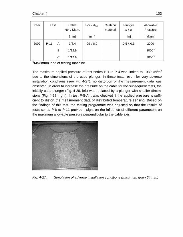
Chapter 4 103
Year Test Cable
No. / Diam.
Soil / dmax Cushion
material
Plunger
b x h
Allowable
Pressure
[mm] [mm] [m] [kN/m2]
2009 P-11 A 3/8.4 G6 / 8.0 - 0.5 x 0.5 2000
B 1/12.9 3000*)
C 1/12.9 3000*)
*)Maximum load of testing machine
The maximum applied pressure of test series P-1 to P-4 was limited to 1030 kN/m2
due to the dimensions of the used plunger. In these tests, even for very adverse
installation conditions (see Fig. 4-27), no distortion of the measurement data was
observed. In order to increase the pressure on the cable for the subsequent tests, the
initially used plunger (Fig. 4-28, left) was replaced by a plunger with smaller dimen-
sions (Fig. 4-28, right). In test P-5-A it was checked if the applied pressure is suffi-
cient to distort the measurement data of distributed temperature sensing. Based on
the findings of this test, the testing programme was adjusted so that the results of
tests series P-6 to P-11 provide insight on the influence of different parameters on
the maximum allowable pressure perpendicular to the cable axis.
Fig. 4-27: Simulation of adverse installation conditions (maximum grain 64 mm)

104 Chapter 4
Fig. 4-28: Plunger 2.0 m x 0.6 m (left) and plunger 0.5 m x 0.5 m (right)
Dependence between pressure and temperature anomaly
The results of test P-9-B confirm the dependency between temperature anomaly and
applied pressure for adverse installation conditions or large pressure. Fig. 4-29
shows the measured temperature and applied pressure against time. It can be clearly
observed that each increase in pressure led to an increase in the measured tempera-
ture. During the load step, temperature decreased, which can be traced back to the
forced controlled loading. While the load remained constant, settlement and crushing
of contact points occurred in the bedding material and led to a redistribution of stress
and consequently to a change in the loading of the fibre optic cable.
Fig. 4-29: Results of laboratory tests P-9-B
Test P-9-B
Time
dT
[ C
]
Com
pre
ssio
n[k
N/m
2]
0
400
800
1200
1600
2000
2400
2800
3200
3600
4000
-28.00
-24.00
-20.00
-16.00
-12.00
-8.00
-4.00
0.00
4.00
8.00
12.00
10:12 10:26 10:40 10:55 11:09
dT Point X1dT Point X2Load
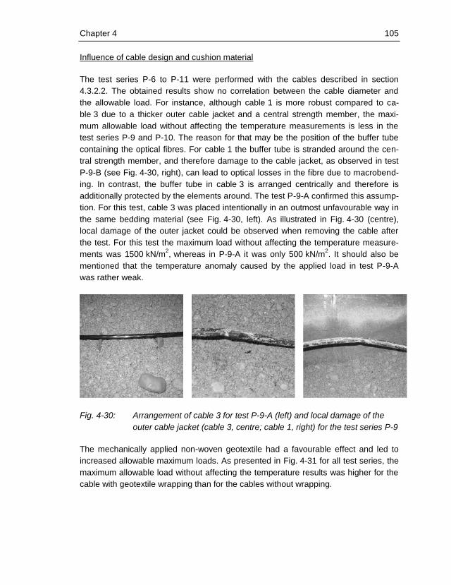
Chapter 4 105
Influence of cable design and cushion material
The test series P-6 to P-11 were performed with the cables described in section
4.3.2.2. The obtained results show no correlation between the cable diameter and
the allowable load. For instance, although cable 1 is more robust compared to ca-
ble 3 due to a thicker outer cable jacket and a central strength member, the maxi-
mum allowable load without affecting the temperature measurements is less in the
test series P-9 and P-10. The reason for that may be the position of the buffer tube
containing the optical fibres. For cable 1 the buffer tube is stranded around the cen-
tral strength member, and therefore damage to the cable jacket, as observed in test
P-9-B (see Fig. 4-30, right), can lead to optical losses in the fibre due to macrobend-
ing. In contrast, the buffer tube in cable 3 is arranged centrically and therefore is
additionally protected by the elements around. The test P-9-A confirmed this assump-
tion. For this test, cable 3 was placed intentionally in an outmost unfavourable way in
the same bedding material (see Fig. 4-30, left). As illustrated in Fig. 4-30 (centre),
local damage of the outer jacket could be observed when removing the cable after
the test. For this test the maximum load without affecting the temperature measure-
ments was 1500 kN/m2, whereas in P-9-A it was only 500 kN/m
2. It should also be
mentioned that the temperature anomaly caused by the applied load in test P-9-A
was rather weak.
Fig. 4-30: Arrangement of cable 3 for test P-9-A (left) and local damage of the
outer cable jacket (cable 3, centre; cable 1, right) for the test series P-9
The mechanically applied non-woven geotextile had a favourable effect and led to
increased allowable maximum loads. As presented in Fig. 4-31 for all test series, the
maximum allowable load without affecting the temperature results was higher for the
cable with geotextile wrapping than for the cables without wrapping.

106 Chapter 4
Fig. 4-31: Influence of the cable design
Influence of maximum grain size and uniformity of the bedding material
For the different test series, bedding materials with a maximum particle size between
3 mm (S 0/3) and 64 mm (G5 0/64) were used. The test results show the influence of
the maximum particle size of the bedding material on the temperature data. It is obvi-
ous that the maximum load which can be allowed without affecting the temperature
data decreases with increasing maximum particle size of the bedding material. In
Fig. 4-32, the maximum loads without influencing the results of the temperature
measurements are plotted against the maximum particle size of the bedding material.
For well graded bedding materials, no influence of the applied load on the tempera-
ture measurements was observed if the maximum particle size was limited to 16 mm.

Chapter 4 107
Fig. 4-32: Maximum load without influencing the measurement results
Therefore, with the test series P-7 and P-10 the influence of uniformity of the bedding
material was investigated. The results confirm the assumption that, for the same
maximum aggregate size, a well graded bedding material is more favourable regard-
ing the maximum allowable load than a uniform bedding material. Punching of the
cable by larger particles is reduced, due to the higher content of fines. For example,
there were significant damages to the cable jacket when using the uniform gravel G7
with a maximum particle size of 16 mm both for cable 1 (Fig. 4-33, left) and cable 3
(Fig. 4-33, centre), while no damages of the cable jacket were observed for the bed-
ding material G1 (Fig. 4-33, right). The relation between the maximum admissible
load and the coefficient of uniformity of the bedding material for the tested cables is
presented in Fig. 4-34.
Fig. 4-33: Damages to the cable jacket
0
500
1000
1500
2000
2500
3000
3500
0 20 40 60 80
m
ax
[kN
/m2]
dmax [mm]
???
Cable 3
Cable 1
Cable 1 + Fleece
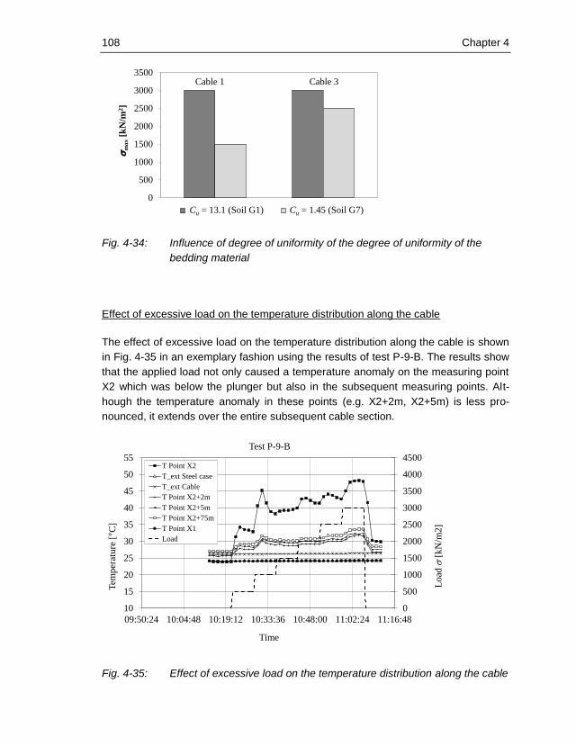
108 Chapter 4
Fig. 4-34: Influence of degree of uniformity of the degree of uniformity of the
bedding material
Effect of excessive load on the temperature distribution along the cable
The effect of excessive load on the temperature distribution along the cable is shown
in Fig. 4-35 in an exemplary fashion using the results of test P-9-B. The results show
that the applied load not only caused a temperature anomaly on the measuring point
X2 which was below the plunger but also in the subsequent measuring points. Alt-
hough the temperature anomaly in these points (e.g. X2+2m, X2+5m) is less pro-
nounced, it extends over the entire subsequent cable section.
Fig. 4-35: Effect of excessive load on the temperature distribution along the cable
Cable 3Cable 1
0
500
1000
1500
2000
2500
3000
3500
m
ax
[kN
/m2]
Influence of Degree of Uniformity dmax = 16 mm
CU =13.2 (Soil G1) CU = 1.5 (Soil G7)Cu = 1.45 (Soil G7)Cu = 13.1 (Soil G1)
0
500
1000
1500
2000
2500
3000
3500
4000
4500
10
15
20
25
30
35
40
45
50
55
09:50:24 10:04:48 10:19:12 10:33:36 10:48:00 11:02:24 11:16:48
Load
[k
N/m
2]
Tem
per
ature
[°C
]
Time
Test P-9-B
T Point X2
T_ext Steel case
T_ext Cable
T Point X2+2m
T Point X2+5m
T Point X2+75m
T Point X1
Load
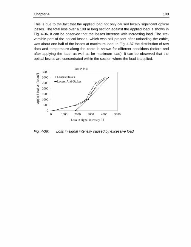
Chapter 4 109
This is due to the fact that the applied load not only caused locally significant optical
losses. The total loss over a 100 m long section against the applied load is shown in
Fig. 4-36. It can be observed that the losses increase with increasing load. The irre-
versible part of the optical losses, which was still present after unloading the cable,
was about one half of the losses at maximum load. In Fig. 4-37 the distribution of raw
data and temperature along the cable is shown for different conditions (before and
after applying the load, as well as for maximum load). It can be observed that the
optical losses are concentrated within the section where the load is applied.
Fig. 4-36: Loss in signal intensity caused by excessive load
0
500
1000
1500
2000
2500
3000
3500
0 1000 2000 3000 4000 5000
Appli
ed l
oad
[k
N/m
2]
Loss in signal intensity [-]
Test P-9-B
Losses Stokes
Losses Anti-Stokes

110 Chapter 4
Fig. 4-37: Optical losses and temperature along cable
Summary of results
The results of the laboratory tests show that pressure perpendicular to the cable axis
can have significant influence on the measuring results of monitoring systems based
on distributed fibre optic temperature measurements. It can be concluded that the
maximum permissible load depends both on the bedding material used and the de-
sign of the fibre optic cable. The geotextile wrapping increases the permissible load.
Additionally a centrically arranged loose tube is beneficial. Based on the results it is
recommended to limit the maximum particle size of the bedding material to 16 mm
and to use well graded material. Whilst bearing these recommendations in mind,
installation of fibre optic cable in dams with a height of up to 75 m should not cause
problems regarding the reliability and accuracy of the measurements. As a result of
the applied loads, damages to the cable sheath occurred and high optical losses led
to distortion of the measurement data. However, the applied loads did not cause the
rupture of the optical fibre in any of the tests. By analysing both, the raw data (optical
losses) and the temperature data, temperature anomalies caused by mechanical
loading can be detected.
20
30
40
50
0
1000
2000
3000
4000
5000
6000
7000
0 10 20 30 40 50 60 70 80 90 100
Tem
per
atu
re [
°C]
Sig
nal
in
ten
sity
(ra
w d
ata)
Station [m]
Test P-9-B
Stokes part before applying load Stokes part at maximum load
Stokes part after unloading Temperature before applying load
Temperature at maximum load Temperature after unloading
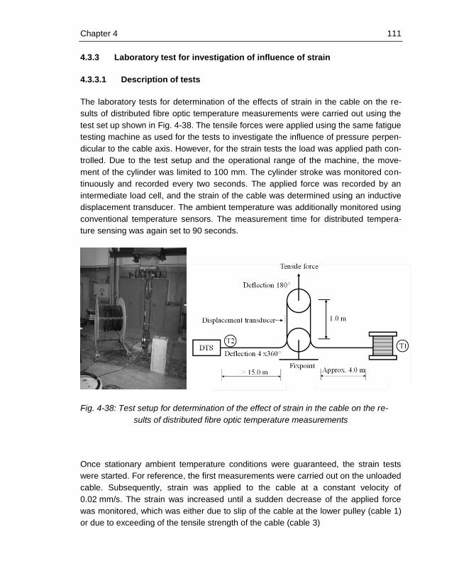
Chapter 4 111
4.3.3 Laboratory test for investigation of influence of strain
4.3.3.1 Description of tests
The laboratory tests for determination of the effects of strain in the cable on the re-
sults of distributed fibre optic temperature measurements were carried out using the
test set up shown in Fig. 4-38. The tensile forces were applied using the same fatigue
testing machine as used for the tests to investigate the influence of pressure perpen-
dicular to the cable axis. However, for the strain tests the load was applied path con-
trolled. Due to the test setup and the operational range of the machine, the move-
ment of the cylinder was limited to 100 mm. The cylinder stroke was monitored con-
tinuously and recorded every two seconds. The applied force was recorded by an
intermediate load cell, and the strain of the cable was determined using an inductive
displacement transducer. The ambient temperature was additionally monitored using
conventional temperature sensors. The measurement time for distributed tempera-
ture sensing was again set to 90 seconds.
Fig. 4-38: Test setup for determination of the effect of strain in the cable on the re-
sults of distributed fibre optic temperature measurements
Once stationary ambient temperature conditions were guaranteed, the strain tests
were started. For reference, the first measurements were carried out on the unloaded
cable. Subsequently, strain was applied to the cable at a constant velocity of
0.02 mm/s. The strain was increased until a sudden decrease of the applied force
was monitored, which was either due to slip of the cable at the lower pulley (cable 1)
or due to exceeding of the tensile strength of the cable (cable 3)
112 Chapter 4
The tests were carried out using cable 1 and cable 3 (see Fig. 4-25).
4.3.3.2 Discussion of the results
The force-deflection diagram of the test for cable 1 is shown in Fig. 4-39 (left). The
maximum observed pulling force was about 30.0 kN (15.0 kN per strand), and the
maximum applied strain was about 1.6%. A further increase of strain or tensile force
was not possible due to slip of the cable at the lower pulley. Yielding of the cable was
not observed during the test. The temperature distributions along the cable for differ-
ent strain states are presented in Fig. 4-39 (right). The section of the cable under
tension is highlighted in green. It became apparent that the temperature anomalies
were mainly caused by bending the cable around the pulleys.
Compared to cable 1, the tensile strength of cable 3 is significantly less, since this
cable has neither a central strength member nor tensile reinforcement. The corre-
sponding force–deflection diagram of the test is shown in Fig. 4-40 (left). For cable 3,
the maximum applied tensile force was 3.0 kN (1.5 kN per cable strand) before the
pulling force decreased to 2.0 kN due to yielding of the cable. Until the operation
range of the hydraulic cylinder was exhausted, the strain in the cable was increased
up to 9.0 % without causing the rupture of the fibre. The temperature distributions
along the cable for different strain states are presented in Fig. 4-40 (right). The sec-
tion of the cable under tension shows significant temperature fluctuations. It can be
observed that the temperature anomalies in this section are mainly caused by optical
losses due to the applied bending diameters at the pulleys and are influenced little by
the strain of the cable. However, the temperature anomalies caused by strain, even
in the event of a large amount of strain on the cable, are small compared to the tem-
perature anomalies caused by compressive stress perpendicular to the cable axis.
Vertical settlement of a dam can cause strain in a fibre optic cable which is placed in
the D/S filter for leakage detection. However, for normal foundation conditions, even
a settlement of two per cent of the height of the dam should not cause strain in the
cable larger than 0.5 ‰. Due to an over length of the fibre and the fact that the fibre
is floating in the loose tube, the strain in the cable is not transferred into the fibre and
therefore normally does not affect the results of DFOT measurements.

Chapter 4 113
Fig. 4-39: Force-deflection diagram and temperature distribution for different strain
states for cable 1
Fig. 4-40: Force-deflection diagram and temperature distribution for different strain
states for cable 3
4.4 Laboratory tests for distributed strain sensing
4.4.1 General
The laboratory tests described in the following were carried out to get a better under-
standing regarding the measuring accuracy, the measuring range and the repeatabil-
ity of distributed fibre optic strain sensing.
-2
-1
0
1
2
15 20 25 30 35 40 45 50 55 60 65 70
dT
[K]
Station [m]
Reference Strain = 0.01% Strain = 0.80% Strain = 1.60%
0
5
10
15
20
25
30
35
0.0 0.5 1.0 1.5 2.0
Fo
rce
[kN
]
Strain [%]
Strained section
-2
-1
0
1
2
15 20 25 30 35 40 45 50 55 60 65 70
dT
[K
]
Station [m]
Reference Strain = 0.01% Strain = 2.7% Strain = 9.0%
0.0
0.5
1.0
1.5
2.0
2.5
3.0
3.5
0 5 10 15
Fo
rce
[kN
]
Strain [%]
Strained section

114 Chapter 4
4.4.2 Description of tests
Testing Facility
The laboratory tests described in the following were carried out at the hydraulic la-
boratory of the University of Innsbruck. The testing facility used for the tests is shown
in Fig. 4-41 and Fig. 4-42. The test setup has already been used by Hoepffner (2008)
to determine the influence of the strained fibre length and the influence of slip be-
tween fibres on the measuring results. The strain rig consists of a 4.0 m long alumini-
um girder with guide rails. At one end of the girder the cable is clamped into a fixed
point, while the other cable fixation is movable. The movable clamp is attached to a
thread rod, which allows application of considerable force to strain the cable during
the tests. The configuration of the strain rig permits the variation of the length of the
strained fibre section between 50 cm and 345 cm. The deformation of the cable is
applied by turning a crank. Due to a reduction gear unit between the crank and the
thread rod, deformations of less than ±0.1 mm can be applied. A distance laser is
also attached to the movable clamp allowing accurate measurements of change in
position up to ±0.01 mm. The measurements are carried out as single end measure-
ments, so that only one end of the cable is connected to the distributed strain system.
For the calibration of the initial state, about 10 m of the cable were placed in a water
basin. To minimize reflections from the free end of the cable into the measuring sec-
tion at least 5 m of cable were left loose after the strain rig. Additionally, several knots
were tied into the cable at the loose end.
Fig. 4-41: Setup for distributed strain sensing laboratory tests (from Hoepffner,
2008)
Thread rod Guide trackStrained fibre section
50 – 345 cm
strain cable
Reduction
Crank lever
l = 4.0 m
Movable
clamp
Fix
clamp
DTSS

Chapter 4 115
Fig. 4-42: Photos of test setup (from Hoepffner, 2008)
Distributed strain sensing system
The instrument used for the laboratory tests presented in section 4.4 was the Sen-
sornetTM DTSS which measures the entire Brillouin spectrum (the Brillouin shift and
power for both the Stokes and the anti-Stokes light). Analysis of these data allows the
strain and temperature to be measured simultaneously and independently at all
points along the fibre. The system is capable of measuring strain and temperature
distributions along optical fibres up to 10 km in length with a strain resolution of
±10 at 1 m intervals and a temperature resolution of ±0.5 K at 1 m intervals.
Tab. 4-12 summarizes the main characteristics of the used device.
A strain value, that is measured, is assumed to be the average strain within the spa-
tial resolution. For post processing, the system carries out several calculations for
more convenient data evaluation. The system has the possibility of integrated tem-
perature compensation by separately evaluating the temperature from the Brillouin
power. The data files provided by the system include, among others, the system
configuration including strain and temperature coefficients, data of attenuation, raw
Brillouin frequency shift along the fibre, uncompensated strain data and temperature
compensated strain data.

116 Chapter 4
Tab. 4-12: Overview DTSS system parameter
Type Measuring
principle
Range Min. spatial
resolution
T
[km] [m] [] [K]
Sensornet DTSS BOTDR 10 1.0 10 0.1
Test procedure
Previous experiments have shown that for distributed fibre optic strain sensing a
sufficiently long strained fibre section is necessary (Hoepffner, 2008). Therefore the
length of the strained fibre section was chosen at 300 cm for the tests. A support
structure made of Perspex was used to prevent the cable from sagging and to pro-
vide similar initial conditions (Fig. 4-43). The initial strain after fixing the cable in the
strain rig, which was used as reference, varied between 500 and 1500 . Addi-
tional strain was applied by moving the movable clamp in steps of 1.0 mm. This cor-
responds to an increase in strain of 333 for the length of the strained fibre section
of 300 cm. For each load step three strain measurements were carried out. The
measuring time for each measurement was set to 2 minutes. If multimode fibres were
provided in the cable, separate distributed fibre optic temperature measurements
were carried out using a DTS system to check the temperature distribution along the
cable.
Fig. 4-43: Support structure to avoid sagging of the cable
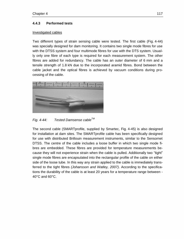
Chapter 4 117
4.4.3 Performed tests
Investigated cables
Two different types of strain sensing cable were tested. The first cable (Fig. 4-44)
was specially designed for dam monitoring. It contains two single mode fibres for use
with the DTSS system and four multimode fibres for use with the DTS system. Usual-
ly only one fibre of each type is required for each measurement system. The other
fibres are added for redundancy. The cable has an outer diameter of 6 mm and a
tensile strength of 1.8 kN due to the incorporated aramid fibres. Bond between the
cable jacket and the optical fibres is achieved by vacuum conditions during pro-
cessing of the cable.
Fig. 4-44: Tested Damsense cableTM
The second cable (SMARTprofile, supplied by Smartec, Fig. 4-45) is also designed
for installation at dam sites. The SMARTprofile cable has been specifically designed
for use with distributed Brillouin measurement instruments, similar to the Sensornet
DTSS. The centre of the cable includes a loose buffer in which two single mode fi-
bres are embedded. These fibres are provided for temperature measurements be-
cause they will not experience strain when the cable is pulled. Additionally two “tight”
single mode fibres are encapsulated into the rectangular profile of the cable on either
side of the loose tube. In this way any strain applied to the cable is immediately trans-
ferred to the tight fibres (Johansson and Watley, 2007). According to the specifica-
tions the durability of the cable is at least 20 years for a temperature range between -
40°C and 60°C.
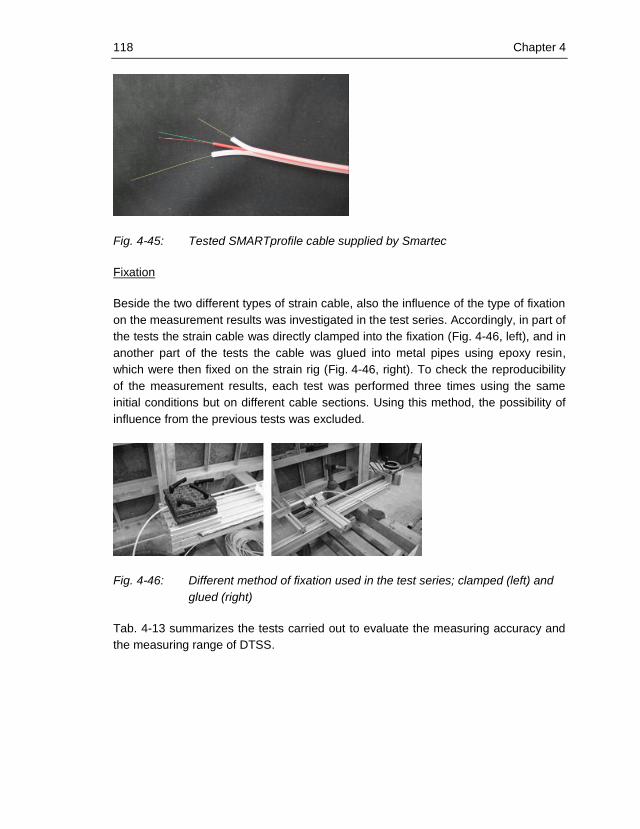
118 Chapter 4
Fig. 4-45: Tested SMARTprofile cable supplied by Smartec
Fixation
Beside the two different types of strain cable, also the influence of the type of fixation
on the measurement results was investigated in the test series. Accordingly, in part of
the tests the strain cable was directly clamped into the fixation (Fig. 4-46, left), and in
another part of the tests the cable was glued into metal pipes using epoxy resin,
which were then fixed on the strain rig (Fig. 4-46, right). To check the reproducibility
of the measurement results, each test was performed three times using the same
initial conditions but on different cable sections. Using this method, the possibility of
influence from the previous tests was excluded.
Fig. 4-46: Different method of fixation used in the test series; clamped (left) and
glued (right)
Tab. 4-13 summarizes the tests carried out to evaluate the measuring accuracy and
the measuring range of DTSS.
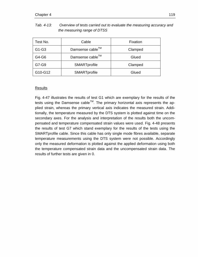
Chapter 4 119
Tab. 4-13: Overview of tests carried out to evaluate the measuring accuracy and
the measuring range of DTSS
Test No. Cable Fixation
G1-G3 Damsense cableTM
Clamped
G4-G6 Damsense cableTM
Glued
G7-G9 SMARTprofile Clamped
G10-G12 SMARTprofile Glued
Results
Fig. 4-47 illustrates the results of test G1 which are exemplary for the results of the
tests using the Damsense cableTM
. The primary horizontal axis represents the ap-
plied strain, whereas the primary vertical axis indicates the measured strain. Addi-
tionally, the temperature measured by the DTS system is plotted against time on the
secondary axes. For the analysis and interpretation of the results both the uncom-
pensated and temperature compensated strain values were used. Fig. 4-48 presents
the results of test G7 which stand exemplary for the results of the tests using the
SMARTprofile cable. Since this cable has only single mode fibres available, separate
temperature measurements using the DTS system were not possible. Accordingly
only the measured deformation is plotted against the applied deformation using both
the temperature compensated strain data and the uncompensated strain data. The
results of further tests are given in 0.

120 Chapter 4
Fig. 4-47: Results of the test G1
Fig. 4-48: Results of the test G7
4.4.4 Analysis of the results
Repeatability of the measuring method
The results of tests with identical initial conditions (i.e. same cable and type of fixa-
Time
DT
S te
mp
erat
ure
[ C
]
Mea
sure
d s
trai
n []
Applied strain []
Compensated strain
Uncompensated strain
Applied strain
Temperature
13:46 16:46 19:46 22:46 01:46 04:46
20
21
22
23
24
0
4000
8000
12000
16000
20000
0 4000 8000 12000 16000
time
DT
S -
tem
per
atu
re [ C
]
mea
sure
d s
train
[m
e]
applied strain [me]
compensated
uncompensated
ideal
Temperatur
13:46 16:46 19:46 22:46 01:46 04:46
20
21
22
23
24
0
4000
8000
12000
16000
20000
0 4000 8000 12000 16000
time
DT
S -
tem
per
atu
re [ C
]
mea
sure
d s
train
[m
e]
applied strain [me]
compensated
uncompensated
ideal
Temperatur
Mea
sure
d s
trai
n []
Applied strain []
Compensated strain
Uncompensated strain
Applied strain
0
4000
8000
12000
16000
20000
0 4000 8000 12000 16000
mea
sure
d s
tra
in [
me]
applied strain [me]
compensated
uncompensated
applied
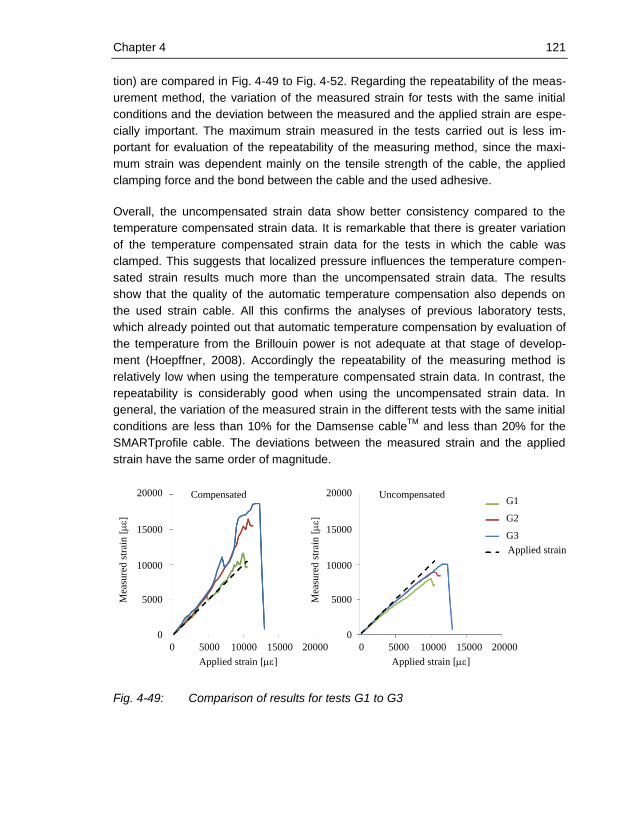
Chapter 4 121
tion) are compared in Fig. 4-49 to Fig. 4-52. Regarding the repeatability of the meas-
urement method, the variation of the measured strain for tests with the same initial
conditions and the deviation between the measured and the applied strain are espe-
cially important. The maximum strain measured in the tests carried out is less im-
portant for evaluation of the repeatability of the measuring method, since the maxi-
mum strain was dependent mainly on the tensile strength of the cable, the applied
clamping force and the bond between the cable and the used adhesive.
Overall, the uncompensated strain data show better consistency compared to the
temperature compensated strain data. It is remarkable that there is greater variation
of the temperature compensated strain data for the tests in which the cable was
clamped. This suggests that localized pressure influences the temperature compen-
sated strain results much more than the uncompensated strain data. The results
show that the quality of the automatic temperature compensation also depends on
the used strain cable. All this confirms the analyses of previous laboratory tests,
which already pointed out that automatic temperature compensation by evaluation of
the temperature from the Brillouin power is not adequate at that stage of develop-
ment (Hoepffner, 2008). Accordingly the repeatability of the measuring method is
relatively low when using the temperature compensated strain data. In contrast, the
repeatability is considerably good when using the uncompensated strain data. In
general, the variation of the measured strain in the different tests with the same initial
conditions are less than 10% for the Damsense cableTM
and less than 20% for the
SMARTprofile cable. The deviations between the measured strain and the applied
strain have the same order of magnitude.
Fig. 4-49: Comparison of results for tests G1 to G3
Applied strain []
Mea
sure
dst
rain
[]
Compensated UncompensatedG1
G2
G3
Applied strain
Mea
sure
dst
rain
[]
Applied strain []
20000
15000
10000
5000
0
0 5000 10000 15000 20000
20000
15000
10000
5000
0
0 5000 10000 15000 20000

122 Chapter 4
Fig. 4-50: Comparison of results for tests G4 to G6
Fig. 4-51: Comparison of results for tests G7 to G9
Applied strain []
Mea
sure
d s
trai
n []
Compensated UncompensatedG4
G5
G6
Applied strain
Mea
sure
d s
trai
n []
Applied strain []
20000
15000
10000
5000
0
0 5000 10000 15000 20000
20000
15000
10000
5000
0
0 5000 10000 15000 20000
Applied strain []
Mea
sure
d s
trai
n []
Compensated Uncompensated
G7
G8
G9
Applied strain
Mea
sure
d s
trai
n []
Applied strain []
20000
15000
10000
5000
0
0 5000 10000 15000 20000
20000
15000
10000
5000
0
0 5000 10000 15000 20000

Chapter 4 123
Fig. 4-52: Comparison of results for tests G10 to G12
Temperature compensation
Brillouin frequency and Brillouin power depend on both temperature and strain.
Therefore temperature correction is recommended if the temperature along the strain
sensing cable is not controlled. In general uncompensated strain data can only be
used for laboratory tests where the temperature can be controlled. The Sensornet
DTSS system provides the option to compensate the strain data for temperature by
using the obtained Brillouin spectrum without additional temperature sensing devices
or reference fibres. Temperature distribution along the cable which is used to com-
pensate the strain data is calculated from the Brillouin power, neglecting the influ-
ence of strain on the Brillouin power. However comparison of the temperature data
obtained from the DTSS system and the DTS system in the strained section of test
G3 spotlights that DTSS temperature data are strain dependent and differ much from
the DTS temperature data (Fig. 4-53). Therefore it is recommended to compensate
the strain data for temperature using the temperature distribution along the strain
cable obtained from DTS measurements. In future the DTSS will be able to retrieve
temperature data directly from the DTS in realtime to provide correction of the data at
the time of measurement and remove the need for any post processing (Johansson
and Watley, 2007).
Applied strain []
Mea
sure
dst
rain
[]
Compensated Uncompensated
G10
G11
G12
Applied strain
Mea
sure
dst
rain
[]
Applied strain []
20000
15000
10000
5000
0
0 5000 10000 15000 20000
20000
15000
10000
5000
0
0 5000 10000 15000 20000
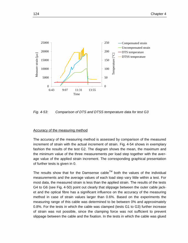
124 Chapter 4
Fig. 4-53: Comparison of DTS and DTSS temperature data for test G3
Accuracy of the measuring method
The accuracy of the measuring method is assessed by comparison of the measured
increment of strain with the actual increment of strain. Fig. 4-54 shows in exemplary
fashion the results of the test G2. The diagram shows the mean, the maximum and
the minimum value of the three measurements per load step together with the aver-
age value of the applied strain increment. The corresponding graphical presentation
of further tests is given in 0.
The results show that for the Damsense cableTM
both the values of the individual
measurements and the average values of each load step vary little within a test. For
most data, the measured strain is less than the applied strain. The results of the tests
G4 to G6 (see Fig. 4-50) point out clearly that slippage between the outer cable jack-
et and the optical fibre has a significant influence on the accuracy of the measuring
method in case of strain values larger than 0.6%. Based on the experiments the
measuring range of this cable was determined to be between 0% and approximately
0.8%. For the tests in which the cable was clamped (tests G1 to G3) further increase
of strain was not possible, since the clamping force was not sufficient to prevent
slippage between the cable and the fixation. In the tests in which the cable was glued
0
50
100
150
200
250
0
5000
10000
15000
20000
25000
6:43 9:07 11:31 13:55
Tem
per
ature
[ C
]
Mea
sure
str
ain []
Time
Compensated strain
Uncompensated strain
DTS temperature
DTSS temperature

Chapter 4 125
to the fixation (tests G4 to G6) tension failure of the cable jacket occurred at a strain
of 0.8%. According to the test results, the accuracy for the Damsense cableTM
is
expected to be ±100 with a resolution of 10 .
In all tests with the SMARTprofile cable in which the cable was clamped, both the
results of the individual measurements and the average values of each load step vary
considerably. For tests in which the cable was glued for fixation the scattering of the
measurement data is significantly less. Based on the test results, the measuring
range for the SMARTprofile cable is expected to be between 0% and 1.5% strain with
an accuracy of ±100 and a resolution of 10 . The measuring range of -1.5%
compressive strain to 1.5% tensile strain, which is specified by the manufacturer, was
confirmed by the tests for the range between 0% and 1.5% strain. In some tests the
maximum applied and measured strain was even larger, as indicated by the results of
test G7 and G10 which had a maximum strain of about 2%. The low maximum strain
in test G12 was due to a failure of the bond between the adhesive and the cable.
Fig. 4-54: Comparison of measured and applied increments of strain for test G2
Evaluation of the tested strain cable
The Damsense cableTM
is lot easier to handle compared to the SMARTprofile cable.
The pigtails with the E2000 connectors were spliced to the optical fibres in the Dam-
sense cableTM
without any problems. Accordingly, repairing the cable on site if dam-
aged can be done easily. Additionally, multimode fibres for separate temperature
measurements are provided in the cable. Due to the softer outer cable jacket the
adverse effects on the measurement results caused by localized excessive pressure
perpendicular to the cable axis, as in the section of the fixation, are less, as well as
0 2 4 6 8 10 12 14 16 18 20 22 24
0
200
400
600
0 2000 4000 6000 8000
Load step
Incr
emen
t o
f st
rain
[]
Total strain []
Max.
Min
Aver.
Applied strain
Max. measured strain increment
Min. measured strain increment
Avg. measured strain increment
Applied strain increment

126 Chapter 4
the scattering of the measured data. Although the tests showed only a measuring
range between 0% and 0.8% strain, it can be assumed that the upper limit of the
measuring range is higher for practical applications. In the case of sufficient bonding
with the surrounding material, it should be in the order of magnitude of the strain at
failure of the optical fibre, which is about 1.5%.
A particular disadvantage of the SMARTprofile cable is that stripping of the material
around the optical fibre is seldom possible afterwards. In the case of damage to the
cable or the connector during installation the whole cable can be lost. Additionally
temperature measurements with common DTS systems which use multimode fibres
are not possible. The tests confirmed the measuring range up to 1.5% strain, howev-
er, the scattering of data was higher compared to the Damsense cableTM
.

Chapter 5 127
5 Recent application examples
5.1 General
Typical examples for the application of leakage detection to monitor hydraulic struc-
tures have already been given in section 3.3.4. Subsequently, using two recent appli-
cation examples, namely the Knezovo dam in Macedonia and the Villalba dam in
Spain, more insights regarding leakage detection in embankment dams with central
core are given. For both dams, the Unit of Hydraulic Engineering of the University of
Innsbruck acted as Consultant for the design and installation of the leakage detection
system.
5.2 Knezovo asphalt core rockfill dam
5.2.1 Situation
The Knezovo Dam is located in the upper stream of the Zletovica River, about 80 km
east of the Macedonian capital Skopje. It is the main element of the Zletovica Basin
Water Utilization Improvement Project with the purpose of water supply, irrigation and
power generation. The Knezovo Dam (Fig. 5-1) is an asphalt core rockfill dam with a
maximum height of 83 m, a crest length of 270 m and a total dam embankment vol-
ume of 1,700,000 m3. The effective storage capacity is 22,500,000 m
3. The instru-
mentation of the dam comprises piezometers, total pressure cells, extensometers
and weirs for measuring the amount of seepage water as well as other devices.
Complementary to the conventional instrumentation, a leakage detection system
based on distributed fibre optic temperature measurements was installed.
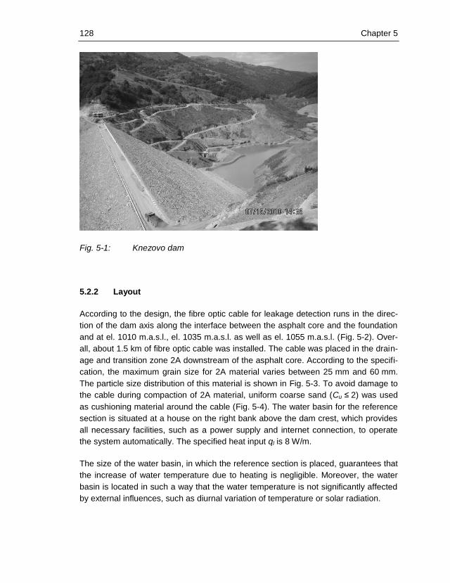
128 Chapter 5
Fig. 5-1: Knezovo dam
5.2.2 Layout
According to the design, the fibre optic cable for leakage detection runs in the direc-
tion of the dam axis along the interface between the asphalt core and the foundation
and at el. 1010 m.a.s.l., el. 1035 m.a.s.l. as well as el. 1055 m.a.s.l. (Fig. 5-2). Over-
all, about 1.5 km of fibre optic cable was installed. The cable was placed in the drain-
age and transition zone 2A downstream of the asphalt core. According to the specifi-
cation, the maximum grain size for 2A material varies between 25 mm and 60 mm.
The particle size distribution of this material is shown in Fig. 5-3. To avoid damage to
the cable during compaction of 2A material, uniform coarse sand (Cu ≤ 2) was used
as cushioning material around the cable (Fig. 5-4). The water basin for the reference
section is situated at a house on the right bank above the dam crest, which provides
all necessary facilities, such as a power supply and internet connection, to operate
the system automatically. The specified heat input ql is 8 W/m.
The size of the water basin, in which the reference section is placed, guarantees that
the increase of water temperature due to heating is negligible. Moreover, the water
basin is located in such a way that the water temperature is not significantly affected
by external influences, such as diurnal variation of temperature or solar radiation.
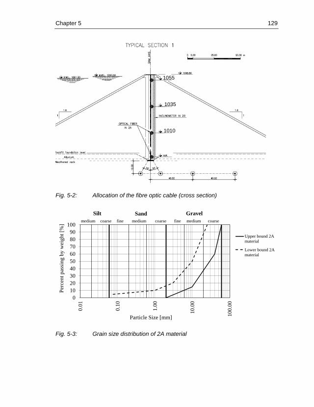
Chapter 5 129
Fig. 5-2: Allocation of the fibre optic cable (cross section)
Fig. 5-3: Grain size distribution of 2A material
1055
1035
1010
0
10
20
30
40
50
60
70
80
90
100
0.0
1
0.1
0
1.0
0
10
.00
10
0.0
0
Per
cen
t p
assi
ng
by
wei
gh
t [%
]
Particle Size [mm]
Upper bound 2A
material
Lower bound 2A
material
Silt Sand Gravel
fine medium coarsefine medium coarsemedium coarse
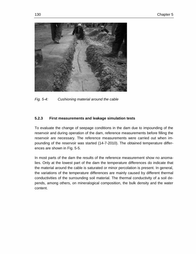
130 Chapter 5
Fig. 5-4: Cushioning material around the cable
5.2.3 First measurements and leakage simulation tests
To evaluate the change of seepage conditions in the dam due to impounding of the
reservoir and during operation of the dam, reference measurements before filling the
reservoir are necessary. The reference measurements were carried out when im-
pounding of the reservoir was started (14-7-2010). The obtained temperature differ-
ences are shown in Fig. 5-5.
In most parts of the dam the results of the reference measurement show no anoma-
lies. Only at the lowest part of the dam the temperature differences do indicate that
the material around the cable is saturated or minor percolation is present. In general,
the variations of the temperature differences are mainly caused by different thermal
conductivities of the surrounding soil material. The thermal conductivity of a soil de-
pends, among others, on mineralogical composition, the bulk density and the water
content.
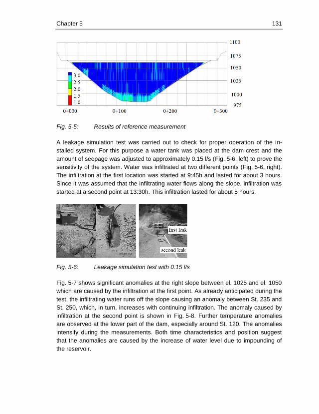
Chapter 5 131
Fig. 5-5: Results of reference measurement
A leakage simulation test was carried out to check for proper operation of the in-
stalled system. For this purpose a water tank was placed at the dam crest and the
amount of seepage was adjusted to approximately 0.15 l/s (Fig. 5-6, left) to prove the
sensitivity of the system. Water was infiltrated at two different points (Fig. 5-6, right).
The infiltration at the first location was started at 9:45h and lasted for about 3 hours.
Since it was assumed that the infiltrating water flows along the slope, infiltration was
started at a second point at 13:30h. This infiltration lasted for about 5 hours.
Fig. 5-6: Leakage simulation test with 0.15 l/s
Fig. 5-7 shows significant anomalies at the right slope between el. 1025 and el. 1050
which are caused by the infiltration at the first point. As already anticipated during the
test, the infiltrating water runs off the slope causing an anomaly between St. 235 and
St. 250, which, in turn, increases with continuing infiltration. The anomaly caused by
infiltration at the second point is shown in Fig. 5-8. Further temperature anomalies
are observed at the lower part of the dam, especially around St. 120. The anomalies
intensify during the measurements. Both time characteristics and position suggest
that the anomalies are caused by the increase of water level due to impounding of
the reservoir.

132 Chapter 5
Fig. 5-7: Results of leakage simulation test at 13:00h
Fig. 5-8: Results of leakage simulation test at 18:00h
5.3 Villalba zoned earthfill dam
5.3.1 Situation
The Villalba de los Barros Dam (Fig. 5-9), for which construction was completed in
2010, is situated in the Guadajira River, about 40 km south of Mérida, in the Guadia-
na River Basin. It forms a reservoir with a capacity of 106 Mio. m3 and a surface of
about 11 km2. The dam is an embankment dam with a clay core and has a maximum
height of 45.50 m and a total length of 450 m. The instrumentation of the dam com-
prises, among others, piezometers, total pressure cells and extensometers. For leak-
age monitoring, a leakage detection system based on fibre optic temperature meas-
urements is installed directly downstream of the central earth core.
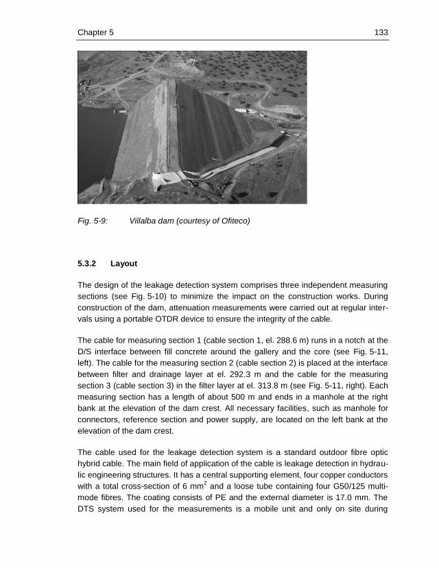
Chapter 5 133
Fig. 5-9: Villalba dam (courtesy of Ofiteco)
5.3.2 Layout
The design of the leakage detection system comprises three independent measuring
sections (see Fig. 5-10) to minimize the impact on the construction works. During
construction of the dam, attenuation measurements were carried out at regular inter-
vals using a portable OTDR device to ensure the integrity of the cable.
The cable for measuring section 1 (cable section 1, el. 288.6 m) runs in a notch at the
D/S interface between fill concrete around the gallery and the core (see Fig. 5-11,
left). The cable for the measuring section 2 (cable section 2) is placed at the interface
between filter and drainage layer at el. 292.3 m and the cable for the measuring
section 3 (cable section 3) in the filter layer at el. 313.8 m (see Fig. 5-11, right). Each
measuring section has a length of about 500 m and ends in a manhole at the right
bank at the elevation of the dam crest. All necessary facilities, such as manhole for
connectors, reference section and power supply, are located on the left bank at the
elevation of the dam crest.
The cable used for the leakage detection system is a standard outdoor fibre optic
hybrid cable. The main field of application of the cable is leakage detection in hydrau-
lic engineering structures. It has a central supporting element, four copper conductors
with a total cross-section of 6 mm2 and a loose tube containing four G50/125 multi-
mode fibres. The coating consists of PE and the external diameter is 17.0 mm. The
DTS system used for the measurements is a mobile unit and only on site during
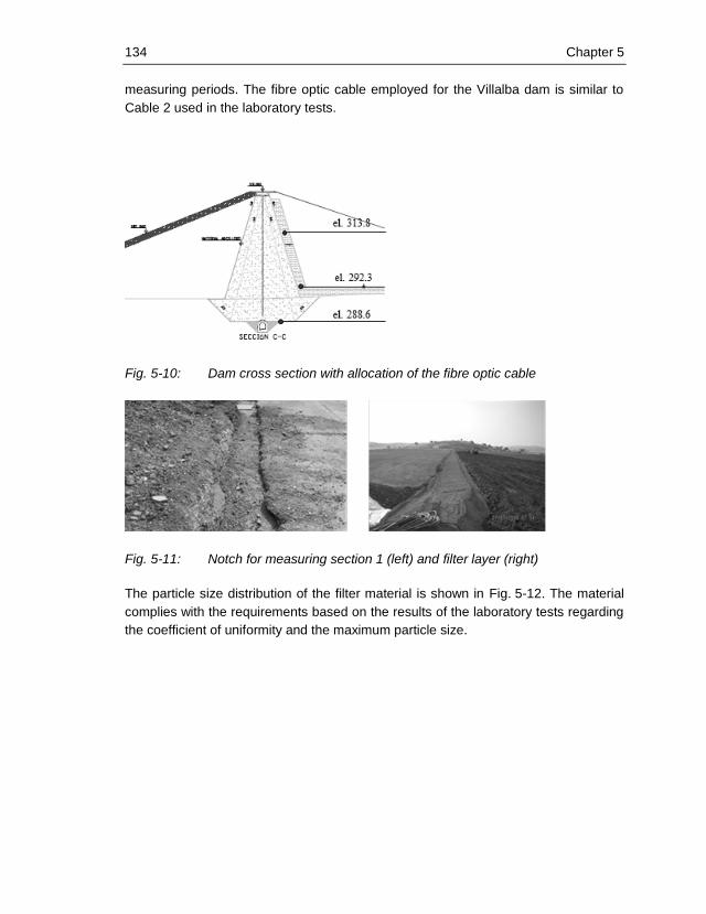
134 Chapter 5
measuring periods. The fibre optic cable employed for the Villalba dam is similar to
Cable 2 used in the laboratory tests.
Fig. 5-10: Dam cross section with allocation of the fibre optic cable
Fig. 5-11: Notch for measuring section 1 (left) and filter layer (right)
The particle size distribution of the filter material is shown in Fig. 5-12. The material
complies with the requirements based on the results of the laboratory tests regarding
the coefficient of uniformity and the maximum particle size.
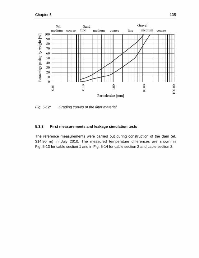
Chapter 5 135
Fig. 5-12: Grading curves of the filter material
5.3.3 First measurements and leakage simulation tests
The reference measurements were carried out during construction of the dam (el.
314.90 m) in July 2010. The measured temperature differences are shown in
Fig. 5-13 for cable section 1 and in Fig. 5-14 for cable section 2 and cable section 3.
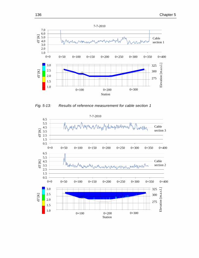
136 Chapter 5
Fig. 5-13: Results of reference measurement for cable section 1
250 250
275 275
300 300
325 325
350
0 + 000 0 + 100 0 + 200 0 + 300 0 + 400
331 331
0+100 0+200 0+300
275
300
325
dT
[K]
0+100 0+150 0+200 0+250 0+300 0+350 0+4000+500+0
2.0
7.06.0
5.0
4.03.0
1.0
dT
[K]
3.0
2.5
2.0
1.5
1.0
7-7-2010
Cable
section 1
Ele
vat
ion
[m
.a.s
.l.]
Station
250 250
275 275
300 300
325 325
350
0 + 000 0 + 100 0 + 200 0 + 300 0 + 400
331 331
0+100 0+200 0+300
275
300
325
dT
[K]
dT
[K]
0+100 0+150 0+200 0+250 0+300 0+350 0+4000+500+0
0+100 0+150 0+200 0+250 0+300 0+350 0+4000+500+0
1.5
6.5
5.5
4.5
3.5
2.5
0.5
1.5
6.5
5.5
4.5
3.5
2.5
0.5
dT
[K]
3.0
2.5
2.0
1.5
1.0
7-7-2010
Cable
section 3
Cable
section 2
Ele
vat
ion
[m
.a.s
.l.]
Station

Chapter 5 137
Fig. 5-14: Results of reference measurement for cable section 2 and cable
section 3
The results of the reference measurement for cable section 1, cable section 2 and
cable section 3, show no anomalies. It can be stated that no flow around the cables
is present. The variations of the temperature differences are mainly caused by differ-
ent thermal conductivities of the surrounding soil material.
As for the Knezovo Dam. a leakage simulation test was carried out to check for prop-
er operation of the installed system. For this purpose a water tank was placed on top
of the filter layer about 1 m above cable section 3. At first the amount of seepage was
adjusted to 0.3 l/s (Fig. 5-15, left) to prove the sensitivity of the system. The infiltra-
tion lasted for about 2 hours. Subsequently, the test was carried out at a second
location with an amount of seepage of 3 l/s (Fig. 5-15, right). This test was main-
tained for approximately 2 hours.
Fig. 5-15: Leakage simulation test with 0.3 l/s (left) and 3.0 l/s (right)
For the small leakage of about 0.3 l/s, the first significant change in temperature
difference is observed at cable section 3 (St. 76.0) approximately 2 h after starting
the infiltration. The anomaly became more pronounced with continuing infiltration
(see Fig. 5-16) and diminished about 2 hours after stopping the infiltration.
Due to the larger amount of seeping water, the infiltration at the second location (St.
85.0) was clearly visible at cable section 3 after about 1 h of infiltration. It took about
2 hours until the infiltration reached cable section 2 (Fig. 5-17).

138 Chapter 5
Fig. 5-16: Results of leakage simulation test at 17:00h
Fig. 5-17: Results of leakage simulation test at 18:00h
250 250
275 275
300 300
325 325
350
0 + 000 0 + 100 0 + 200 0 + 300 0 + 400
331 331
0+100 0+200 0+300
275
300
325
8-7-2010 17:00h
dT
[K]
0+100 0+150 0+200 0+250 0+300 0+350 0+4000+500+0
1.5
5.5
4.5
3.5
2.5
0.5
dT
[K]
0+100 0+150 0+200 0+250 0+300 0+350 0+4000+500+0
1.5
5.5
4.5
3.5
2.5
6.5
0.5
6.5
dT
[K]
3.0
2.5
2.0
1.5
1.0
Cable
section 3
Cable
section 2
Ele
vat
ion
[m
.a.s
.l.]
Station
250 250
275 275
300 300
325 325
350
0 + 000 0 + 100 0 + 200 0 + 300 0 + 400
331 331
0+100 0+200 0+300
275
300
325
dT
[K]
dT
[K]
dT
[K]
8-7-2010 18:00h
0+100 0+150 0+200 0+250 0+300 0+350 0+4000+500+0
0+100 0+150 0+200 0+250 0+300 0+350 0+4000+500+0
1.5
5.5
4.5
3.5
2.5
1.5
5.5
4.5
3.5
2.5
6.5
0.5
6.5
3.0
2.5
2.0
1.5
1.0
Cable
section 3
Cable
section 2
Ele
vat
ion
[m
.a.s
.l.]
Station
Chapter 5 139
5.4 Remarks on the planning of leakage detection systems
5.4.1 Factors that can cause defects in the sealing elements
In order to ensure the adjustment of the monitoring system in regard to the character-
istics and peculiarities of the dam, the planning of the leakage detection system
should be carried out in close cooperation with the professionals in charge of the
design of the dam. In regard to leakage detection, it is important to consider the fac-
tors which can lead to defects in the sealing elements, and to assess the likelihood of
their occurrence. Defects in the sealing element can be concentrated leaks or zones
of high permeability. In many cases, such defects initiate internal erosion of the dam.
The factors which may lead to defects in the sealing system are discussed in detail in
(Foster et al., 2000b).
By means of numerical analysis of the stress and deformation conditions, it may be
possible to predict low stress zones which are likely to result in transverse cracking
(Bui et al., 2005). These low stress zones may be due to hydraulic fracturing or are
caused by the topography of the dam site. Such information is especially important
for the planning of system because the arrangement of the fibre optic cable can be
adjusted in such a way that monitoring of potential low stress zones is possible.
5.4.2 Frequency of measurements
Each measuring cycle for leakage detection should comprise of temperature meas-
urements of about half an hour while the cable is in an unheated state. The cable is
heated then with the specified heat input, which, for leakage detection, is generally
about one hour. The temperature differences are calculated using the average tem-
perature in the unheated state and the average temperature measured during the
last 10 minutes of the heating period. Based on the experience obtained from labora-
tory tests, it can be assumed that for saturated soils, steady state temperature distri-
bution is obtained at the latest six hours after disconnection of the heating. Therefore,
two measuring cycles for leakage detection per day are considered to be realistic.
Furthermore, to guarantee comparability of measurement data of different instru-
ments and different measuring methods, the measuring cycles for leakage detection
should be coordinated with the measurements of pore pressure, quantity of seepage
water and water level in the reservoir based on the information given in the monitor-
ing program of the dam. If possible, all these measurements should be carried out
automatically. In case of abnormal reservoir levels, abnormal measurement results or
observations as well as after earthquakes additional measurements should be carried
out.
140 Chapter 5
5.5 Remarks on the determination of critical flow velocity
If soils are present, which are especially susceptible to suffusion, the likelihood of
particle transport can be assessed by comparing the filter velocities derived from the
measured temperature differences with the critical velocity causing transport of parti-
cles.
In order to carry out an assessment of the critical filter velocity, in a first step the size
of the largest erodible particle should be estimated by using an appropriate geometric
criterion. In the following, the approach is described exemplarily by using the particle
size distribution curve of an internally unstable soil tested by Wan and Fell (2004).
The particle size distribution curve is divided into a primary fabric (coarse fractions)
and into potentially mobile particles (fine fractions) at the inflection point of the gap
gradation. Fig. 5-18 presents particle size distribution of the investigated soil sample,
the particle size distribution of the coarse fraction and the fine fraction as well as the
pore constriction size distribution for the dense state and the loose state. The latter
has been calculated with the approach presented in section 2.1.2.2. According to
Semar and Witt (2008), the diameter with the cumulative frequency of pcrit = 0.75 is
the largest erodible particle.
Fig. 5-18: Calculated pore constriction size distribution and size of largest erodi-
ble particle
The critical velocity wcrit, which is causing or sustaining particle transport, can be
assessed by using the equations for explicit calculation of the particle settling velocity
0
10
20
30
40
50
60
70
80
90
100
0.0
01
0.0
10
0.1
00
1.0
00
10.0
00
100.0
00
Per
cent
pas
sing b
y w
eight
[%]
Particle size [mm]
Soil A2
Mobile particles
CSD dense
CSD loose
Primary fabric
Silt Sand Gravel
fine medium coarsefine medium coarsemedium coarsefine
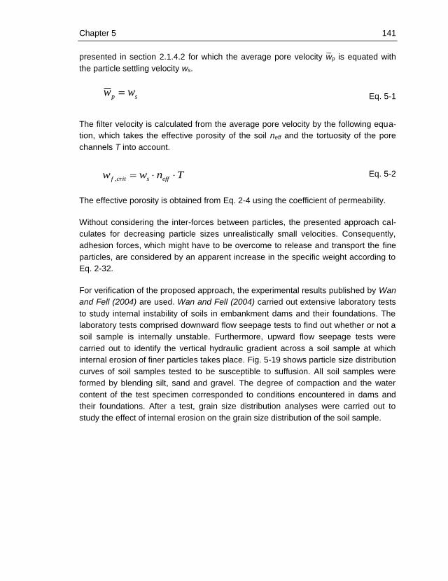
Chapter 5 141
presented in section 2.1.4.2 for which the average pore velocity w̄p is equated with
the particle settling velocity ws.
sp ww Eq. 5-1
The filter velocity is calculated from the average pore velocity by the following equa-
tion, which takes the effective porosity of the soil neff and the tortuosity of the pore
channels T into account.
Tnww effscritf , Eq. 5-2
The effective porosity is obtained from Eq. 2-4 using the coefficient of permeability.
Without considering the inter-forces between particles, the presented approach cal-
culates for decreasing particle sizes unrealistically small velocities. Consequently,
adhesion forces, which might have to be overcome to release and transport the fine
particles, are considered by an apparent increase in the specific weight according to
Eq. 2-32.
For verification of the proposed approach, the experimental results published by Wan
and Fell (2004) are used. Wan and Fell (2004) carried out extensive laboratory tests
to study internal instability of soils in embankment dams and their foundations. The
laboratory tests comprised downward flow seepage tests to find out whether or not a
soil sample is internally unstable. Furthermore, upward flow seepage tests were
carried out to identify the vertical hydraulic gradient across a soil sample at which
internal erosion of finer particles takes place. Fig. 5-19 shows particle size distribution
curves of soil samples tested to be susceptible to suffusion. All soil samples were
formed by blending silt, sand and gravel. The degree of compaction and the water
content of the test specimen corresponded to conditions encountered in dams and
their foundations. After a test, grain size distribution analyses were carried out to
study the effect of internal erosion on the grain size distribution of the soil sample.
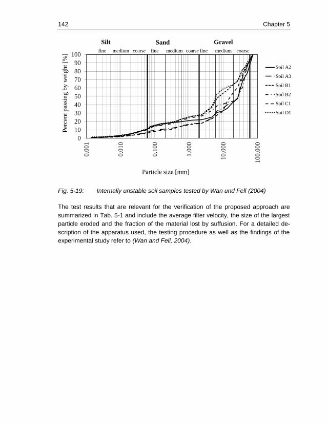
142 Chapter 5
Fig. 5-19: Internally unstable soil samples tested by Wan und Fell (2004)
The test results that are relevant for the verification of the proposed approach are
summarized in Tab. 5-1 and include the average filter velocity, the size of the largest
particle eroded and the fraction of the material lost by suffusion. For a detailed de-
scription of the apparatus used, the testing procedure as well as the findings of the
experimental study refer to (Wan and Fell, 2004).
0
10
20
30
40
50
60
70
80
90
100
0.0
01
0.0
10
0.1
00
1.0
00
10
.00
0
10
0.0
00
Per
cen
t p
assi
ng
by
wei
gh
t [%
]
Particle size [mm]
Soil A2
Soil A3
Soil B1
Soil B2
Soil C1
Soil D1
Silt Sand Gravel
fine medium coarsefine medium coarsemedium coarsefine
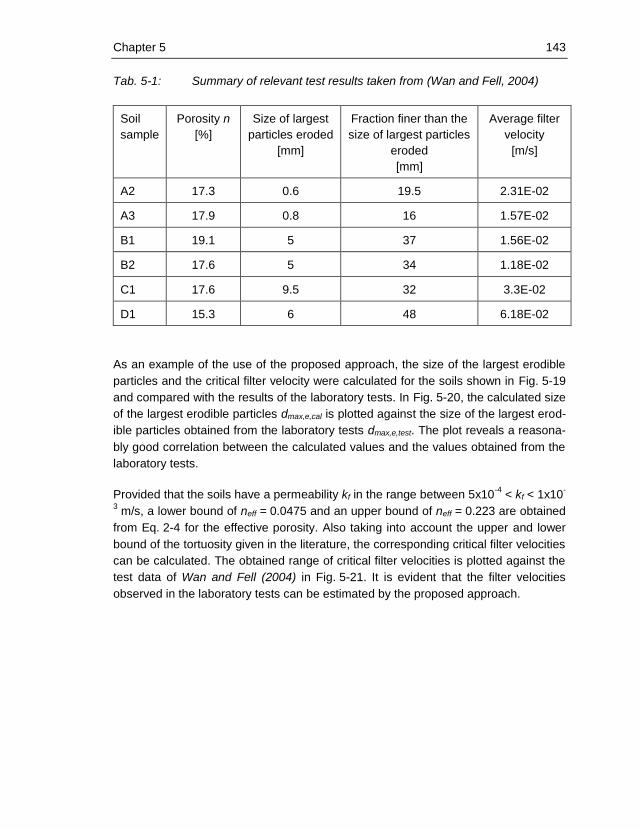
Chapter 5 143
Tab. 5-1: Summary of relevant test results taken from (Wan and Fell, 2004)
Soil
sample
Porosity n
[%]
Size of largest
particles eroded
[mm]
Fraction finer than the
size of largest particles
eroded
[mm]
Average filter
velocity
[m/s]
A2 17.3 0.6 19.5 2.31E-02
A3 17.9 0.8 16 1.57E-02
B1 19.1 5 37 1.56E-02
B2 17.6 5 34 1.18E-02
C1 17.6 9.5 32 3.3E-02
D1 15.3 6 48 6.18E-02
As an example of the use of the proposed approach, the size of the largest erodible
particles and the critical filter velocity were calculated for the soils shown in Fig. 5-19
and compared with the results of the laboratory tests. In Fig. 5-20, the calculated size
of the largest erodible particles dmax,e,cal is plotted against the size of the largest erod-
ible particles obtained from the laboratory tests dmax,e,test. The plot reveals a reasona-
bly good correlation between the calculated values and the values obtained from the
laboratory tests.
Provided that the soils have a permeability kf in the range between 5x10⁻⁴
< kf < 1x10-
3 m/s, a lower bound of neff = 0.0475 and an upper bound of neff = 0.223 are obtained
from Eq. 2-4 for the effective porosity. Also taking into account the upper and lower
bound of the tortuosity given in the literature, the corresponding critical filter velocities
can be calculated. The obtained range of critical filter velocities is plotted against the
test data of Wan and Fell (2004) in Fig. 5-21. It is evident that the filter velocities
observed in the laboratory tests can be estimated by the proposed approach.
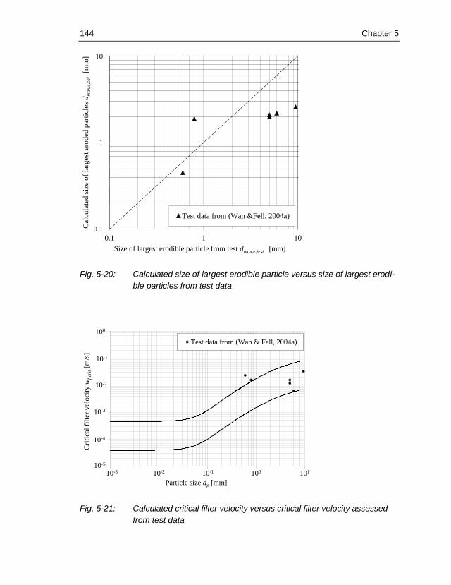
144 Chapter 5
Fig. 5-20: Calculated size of largest erodible particle versus size of largest erodi-
ble particles from test data
Fig. 5-21: Calculated critical filter velocity versus critical filter velocity assessed
from test data
0.1
1
10
0.1 1 10
Cal
cula
ted
siz
e o
f la
rges
t er
oded
par
ticl
es d
ma
x,e,
cal
[mm
]
Size of largest erodible particle from test dmax,e,test [mm]
Test data from (Wan &Fell, 2004a)
1.00E-05
1.00E-04
1.00E-03
1.00E-02
1.00E-01
1.00E+00
0.001 0.01 0.1 1 10
Test data from (Wan & Fell, 2004a)
Particle size dp [mm]
10-3 10-2 10-1 100 10110-5
10-4
10-3
10-2
10-1
100
Cri
tica
l fi
lter
vel
oci
ty w
f,cr
it[m
/s]

Chapter 5 145
The hydraulic criterion after Muckenthaler (1989) as well as the modified approach
presented in section 2.1.4.3 imply a tubular erosion channel with a minimum diameter
of around 30 mm. Since such defects are not typical for suffusion processes, the use
of these criteria is not recommended in this context.

146 Chapter 5
Chapter 6 147
6 Summary and conclusions
6.1 Distributed fibre optic temperature sensing
The presented thesis deals with the application of distributed fibre optic measure-
ments in order to provide additional data for assessment of the safety of embankment
dams regarding leakage and internal erosion. The detection of internal erosion pro-
cesses by means of measurement data generally requires both detailed knowledge
of the structure, which is monitored, and sound subject-specific theoretical
knowledge. Consequently, beside the findings of laboratory tests, the theoretical
backgrounds of the relevant geohydraulic processes as well as a description of inter-
nal erosion processes in embankment dams with impervious cores are part of this
thesis.
Based on existing approaches to describe the geometry of the pore structure of
granular soils by simplified parameters, a method to estimate the size of the largest
erodible particle in suffosive soils is presented. By applying this method to soils,
which were studied in laboratory tests by Wan and Fell (2004) and found to be suf-
fosive, the applicability of the method could be confirmed. Furthermore, the ap-
proaches to determine the critical filter velocity causing transport of fine particles
were reviewed. Based on the findings of the literature review, the iterative calculation
of the particle settling velocity using the equation of Kazanskij (1981) was replaced
by an explicit calculation with the empirical equations proposed by Cheng (2008a).
The hydraulic criterion of Muckenthaler (1989), which is based on approaches gener-
ally used to describe sediment transport, was reviewed in detail and checked for its
applicability. The original hydraulic criterion was simplified by replacing the equations
after Zanke (1982), which describe the relationship between Shields factor c and the
Reynolds number, as well as the relationship between the critical shear velocity w*
and the particle size with equations proposed by Paphitis (2001), which are based on
a large amount of published experimental data. Moreover, the equation to calculate
the friction factor for rough pipes by Colebrook and White was replaced by the
explicit equation after Cheng (2008b). In this context it should be pointed out that the
hydraulic criterion as presented in (Muckenthaler, 1989) calculates only the local
critical velocity. However, in order to assess if particle transport takes place or not, it
is necessary to equate the mean effective pore velocity w̄p with the mean velocity in
the pipe w̄ at onset of particle transport. Therefore, the original approach was com-
plemented by the formulas of Schlichting (1965) to calculate the mean velocities in
turbulent pipe flows. It should be noted that this hydraulic criterion assumes as
straight tubular pore channel or defect, for which the diameter depends on the
roughness of the pipe. Due to the equations used, the diameter is 15 times the
roughness, i.e. for a roughness of 1 mm the diameter is 15 mm. Since on one hand

148 Chapter 6
this hydraulic criterion is only applicable for granular soils, however, on the other
hand granular soils rarely exhibit such types of defects, general application of the
criterion is not possible. Therefore, according to current knowledge, the approach
based on the particle settling velocity should be used to estimate the critical seepage
velocity causing transport of fine particles. Comparison of calculated critical velocities
with experimental data published by Wan and Fell (2004) revealed a reasonably
good correlation.
Laboratory tests were carried out in order to prove the applicability and general func-
tioning of distributed fibre optic temperature measurements under conditions in which
the fibre optic cable is exposed to strain and pressure perpendicular to the cable axis.
Based on the findings of these tests, it can be concluded that loads due to overbur-
den pressure can have a significant influence on the data of distributed fibre optic
temperature measurements. Since the allowable overburden pressure, which does
not affect the measurement data, depends also on the material around the cable, it is
recommended to use well-graded material with a maximum particle size of 16 mm
around the cable. Additionally, the experiments have shown that for normal founda-
tion conditions, the influence of strain on the measurement data due to settlement of
the dam is not significant.
The laboratory tests for leakage detection and filter velocity measurements with dif-
ferent fibre optic cables confirmed the assumption that the accuracy of the measuring
method increases with decreasing cable diameters. However, when selecting the
type of heat-up cable for specific projects, the measuring accuracy and the require-
ments for strength and robustness of the cable must always be taken into account.
An important aspect of this work is the practical application of distributed fibre optic
measurements in embankment dams. Hence two recent application examples for
leakage detection systems in embankment dams with central cores are presented
and first measurement results are discussed. In addition, general remarks on the
planning of leakage detection systems are given.
Currently, the leakage detection system based on distributed fibre optic temperature
measurements installed at the Knezovo Dam in Macedonia is converted into a per-
manent monitoring system. Once the system is fully operational, concepts based on
the recorded data should be developed to efficiently detect and locate both short-
term changes and long-term changes in the seepage behaviour of the dam. In addi-
tion, using the testing facility in the hydraulic laboratory of the Innsbruck University,
the automation of the monitoring system should be advanced. Further development
of the system should focus especially on the data analysis and the integration of data
obtained from other instruments in the evaluation, such as measurement of pore

Chapter 6 149
pressure, quantity of seepage water and water level in the reservoir.
6.2 Distributed fibre optic temperature and strain sensing
Research and development in the field of distributed fibre optic strain sensing based
on Brillouin optical time domain reflectometry is making great progress. Methods for
reducing the spatial resolution and more accurate temperature compensation of the
strain data are under development or being tested. Therefore, steady improvement of
the measuring instruments can be expected.
The experimental results have shown that the design of the strain cable and the
installation of the cable are decisive for successful accomplishment of the measure-
ments. Furthermore, the laboratory tests revealed that the automatic temperature
compensation by evaluating the temperature from the Brillouin power is not adequate
at the present stage of development. Therefore, it is recommended to use DTS tem-
perature data obtained from the same cable to compensate the strain data for tem-
perature. Based on the results, the conclusion can be drawn that the sensitivity of
distributed strain sensing is high and deviation of the measured strain from the ap-
plied strain was less than 20% in the performed tests. The repeatability of distributed
fibre optic strain sensing is good. If movements could effectively be transferred into
the fibre, the measuring range is limited by the strain at failure of the fibre, which is
1.5% or more. The design of the cable must guarantee the transfer of strain from the
cable coating to the optical fibre but also allow easy installation of connectors and
repair of damaged cable sections. In addition, the cable must be robust enough for
installation in soil. Furthermore, the optical fibres in the cable must be compatible
with the monitoring system used.
Altogether, the results of the laboratory tests are positive. Considering the current
state of technology, the potential of distributed fibre optic strain sensing is seen more
in the accomplishment of new measuring tasks, such as detection of low stress
zones or sinkholes, rather than in the replacement of the measuring methods used so
far for measuring deformations. The next step in order to prove the suitability of dis-
tributed fibre optic strain sensing for monitoring of embankment dams would be the
installation of strain sensing cables in a trial embankment. This embankment should
be designed and constructed in such a way that differential settlement occurs. This
would contribute to the clarification of whether the accuracy of the measurement
method is sufficient to detect areas of differential deformation behaviour in situ. Addi-
tionally, based on the findings of the laboratory tests in cooperation with a cable
manufacturer, the design of the strain sensing cable could be improved.

150 Chapter 6

Bibliography 151
Bibliography
ANCOLD 2003. Guidelines on dam safety management. Australian National Commit-
tee on Large Dams, Melbourne.
ARMBRUSTER, H., BLINDE, A., BRAUNS, J., DÖSCHER, H., HÖTZL, H. &
MERKLER, G. 1989. The application of geoelectrical and thermal meas-
urements to locate dam leakages. In: MERKLER, G.-P., MILITZER, H.,
HÖTZL, H., ARMBRUSTER, H. & BRAUNS, J. (eds.) Detection of Subsur-
face Flow Phenomena. Springer Berlin / Heidelberg.
ARMBRUSTER, H., DORNSTÄDTER, J., KAPPELMEYER, O. & TRÖGER, I. 1993.
Thermometrie zur Erfassung von Schwachstellen an Dämmen. Wasserwirt-
schaft, Vol. 83 (4).
AUFLEGER, M. 2000. Verteilte faseroptische Temperaturmessungen im Wasserbau.
Lehrstuhl und Versuchsanstalt für Wasserbau und Wasserwirtschaft, Tech-
nische Universität München, Bericht Nr. 89.
AUFLEGER, M., CONRAD, M. & GOLTZ, M. 2007a. Distributed fibre optic tempera-
ture measurements – a competitive alternative for temperature monitoring in
large RCC dams. In: Proceedings of the 5th International Symposium on
RCC Dams, Guiyang, China, November 2-4.
AUFLEGER, M., CONRAD, M., PERZLMAIER, S. & PORRAS, P. 2005. Improving a
fibre optics tool for monitoring leakage. HRW, Vol. 13, pp. 18- 23.
AUFLEGER, M., DORNSTÄDTER, J., STROBL, T., CONRAD, M., PERZLMAIER, S.
& GOLTZ, M. 2007b. 10 Jahre verteilte faseroptische Temperaturmessun-
gen im Wasserbau. Wasserwirtschaft.
BAEHR, H. D. & STEPHAN, K. 1994. Wärme- und Stoffübertragung, Berlin, Springer-
Verlag.
BEAR, J. 1972. Dynamics of fluids in porous media, New York, American Elsevier.
BEYER, W. & SCHWEIGER, K.-H. 1969. Zur Bestimmung des entwässerten Poren-
anteils der Grundwasserleiter. Wasserwirtschaft-Wassertechnik, 19, No. 2,
pp. 57-60.
BIESKE, E. 1992. Bohrbrunnen, München, Oldenburg.
BROWN, P. P. & LAWLER, D. F. 2003. Sphere drag and settling velocity revisited.
Journal of Environmental Engineering, Vol. 129, 222-231.
BUI, H. N., TANDJIRIA, V., FELL, R., SONG, C. & KHALILI, N. 2005. Two and three
dimensional numerical analysis of the potential for cracking of embankment
dams during construction - Supplementary Report. UNICIV report No. R-
438, University of New South Wales, School of Civil and Environmental En-
gineering, Sydney
BURCHARTH, H. F. & ANDERSEN, O. K. 1995. On the one-dimensional steady and
unsteady porous flow equations. Coastal Engineering, 24, 233-257, Doi:
152 Bibliography
10.1016/0378-3839(94)00025-s.
BUSCH, K.-F. & LUCKNER, L. 1974. Geohydraulik für Studium und Praxis, 2. Aufla-
ge, Stuttgart, Enke.
BUTLER, D. 1989. Geophysical methodology for subsurface fluid flow detection,
mapping and monitoring: An overview and selected case history. In:
MERKLER, G.-P., MILITZER, H., HÖTZL, H., ARMBRUSTER, H. &
BRAUNS, J. (eds.) Detection of Subsurface Flow Phenomena. Springer
Berlin / Heidelberg.
CARLSTEN, S., JOHANSSON, S. & WÖRMAN, A. 1995. Radar techniques for indi-
cating internal erosion in embankment dams. Journal of Applied Geophys-
ics, 33, 143-156, Doi:10.1016/0926-9851(95)90037-3.
CARMAN, P. C. 1938. The determination of the specific surface of powders. J. Soc.
Chem. In. Trans., 57, 225.
CARMAN, P. C. 1956. Flow of gases through porous media, London, Butterworths
Scientific Publications.
CARRIER, W. D. 2003. Goodbye, Hazen; Hello, Kozeny-Carman. Journal of Ge-
otechnical and Geoenvironmental Engineering, Vol. 129, 1054-1056.
CHENG, N. 2008a. Comparison of formulas for drag coefficient and settling velocity
of spherical particles. Powder Technology, doi:
10.1016/j.powtec.2008.07.0006.
CHENG, N. 2008b. Formulas for friction factor in transitional regimes. Journal of
Hydraulic Engineering, Vol. 134, 1357-1362.
CHENG, N. S. 1997. Simplified settling velocity formula for sediment particle. Journal
of Hydraulic Engineering-Asce, 123, 149-152.
DORNSTÄDTER, J. 1997. Detection of internal erosion in embankment dams. 19th
Congress on Large Dams, Florence.
DORNSTÄDTER, J. & AUFLEGER, M. 1998. Distributed temperature sensing in
dams – the prospect for reservoirs in the 21st century. In: Proceedings of
the 10th Conference of British Dam Society, University of Wales, Bangor.
DWA 2008. Merkblatt DWA-M514 Bauwerksüberwachung an Talsperren (Gelb-
druck). Deutsche Vereinigung für Wasserwirtschaft, Abwasser und Abfall
e.V. .
ETZER, T. 2010. Ein Beitrag zur Beurteilung der hydraulischen Sicherheit von Stau-
dämmen. Arbeitsbereich Wasserbau, Universität Innsbruck.
FAND, R. M., KIM, B. Y. K., LAM, A. C. C. & PHAN, R. T. 1987. Resistance to the
flow of fluids through simple and complex porous media whose matrices are
composed of randomly packed spheres. Trans. ASME, J. Heat and Mass
Transfer, 30, pp. 1351-1358.
FAND, R. M., VARAHASAMY, M. & GREER, L. S. 1993. Empirical correlation equa-
tion for heat transfer by forced convection from cylinders embedded in po-
rous media that accounts for wall effects and dispersion. Int. J. Heat and
Mass Transfer, Vol. 36, pp. 4407-4418.

Bibliography 153
FANNIN, R. J. & GARNER, S. J. 2010. Understanding internal erosion: a decade of
research following a sinkhole event. International Journal on Hydropower
and Dams, 17 (3), pp. 93-98.
FAROUKI, O. T. 1986. Thermal properties of soil. Trans Tech Publications, Series on
Rock and Soil Mechanics, Vol. 11.
FELL, R. & FRY, J.-J. 2007. The state of the art of assessing the likelihood of internal
erosion of embankment dams, water retaining structures and their founda-
tions. In: FELL, R. & FRY, J.-J. (eds.) Internal erosion of dams and their
foundation. London: Taylor & Francis.
FELL, R., MACGREGOR, P., STAPLEDON, D. & BELL, G. 2005. Geotechnical engi-
neering of dams, A.A. Balkema Publishers.
FELL, R. & WAN, C. F. 2005. Methods for estimating the probability of failure of em-
bankment dams by internal erosion and piping in the foundation and from
the embankment to the foundation. UNICIV Report No. R-436, University of
New South Wales, School of Civil and Environmental Engineering, Sydney.
FELL, R., WAN, C. F., CYGANIEWICZ, J. & FOSTER, M. A. 2001. The time for de-
velopment and detectability of internal erosion and piping in embankment
dams and their foundations. UNICIV Report No. R-399, University of New
South Wales, School of Civil and Environmental Engineering, Sydney.
FELL, R., WAN, C. F. & FOSTER, M. A. 2004. Methods for estimating the probability
of failure of embankment dams by internal erosion and piping : piping
through the embankment / by Robin Fell, Chi Fai Wan and Mark Foster.
UNICIV Report No. R-428, University of New South Wales, School of Civil
and Environmental Engineering, Sydney :.
FORCHHEIMER, P. 1930. Hydraulik, 3. Auflage, Leipzig und Berlin, B. G. Teubner.
FOSTER, M. A. 1999. The probability of failure of embankment dams by internal
erosion and piping. School of Civil and Environmental Engineering, Universi-
ty of New South Wales, Sydney, Australia.
FOSTER, M. A. & FELL, R. 1999a. Assessing embankment dam filters which do not
satisfy design criteria UNICIV Report No. R-376, University of New South
Wales, School of Civil and Environmental Engineering, Sydney
FOSTER, M. A. & FELL, R. 1999b. A Framework for estimating the probability of
failure of embankment dams by internal erosion and piping using event tree
methods. UNICIV Report No. R-377, University of New South Wales, School
of Civil and Environmental Engineering, Sydney
FOSTER, M. A., FELL, R. & SPANNAGLE, M. 2000a. A method for estimating the
relative likelihood of failure of embankment dams by internal erosion and
piping. Canadian Geotechnical Journal, 37, 1025-1061.
FOSTER, M. A., FELL, R. & SPANNAGLE, M. 2000b. Use of event trees to estimate
the probability of failure of embankment dams by internal erosion and pip-
ing. 20th Int. Congress on Large Dams, Beijing, China.
FRIVIK, P. E., THORSBERGSEN, E., DEL GUIDICE, S. & COMINI, G. 1977. Ther-
154 Bibliography
mal design of pavement structures in seasonal frost areas. Journal of Heat
Transfer, Vol. 99, pp. 533-540.
GAFFRAN, P. & JEFFRIES, M. 2005. A study of through-dam seismic testing at
WAC Bennet Dam. CEATI, Montreal, Quebec, Canada.
HAZEN, A. 1892. Some physical properties of sands and gravel, with special refer-
ence to their use in filtration. Massachusetts State Board of Health, 24th
Annual Report, Boston, 539-556.
HAZEN, A. 1911. Discussion: Dams on sand foundation. Transactions of the Ameri-
can Society of Civil Engineers, Vol. 73, 199-203.
HILL, R. J. & KOCH, D. L. 2002. The transition from steady to weakly turbulent flow
in a closed-packed ordered array of spheres. Journal of Fluid Mechanics,
Vol. 465, 59-97.
HOEPFFNER, R. 2008. Distributed fibre optic strain sensing in hydraulic concrete
and earth structures. Lehrstuhl und Versuchsanstalt für Wasserbau und
Wasserwirtschaft, Technische Universität München, Bericht Nr. 121.
HUGHES, A. 2010. A simple experience with new means of leakage detection. In:
Proceedings of the 8th European Club Symposium, Innsbruck, Austria.
HUNTER, G. & FELL, R. 2003. Rockfill Modulus and Settlement of Concrete Face
Rockfill Dams. Journal of Geotechnical and Geoenvironmental Engineering,
129, pp. 909-917.
INDRARATNA, B., RAUT, A. K. & KHABBAZ, H. 2007. Constriction-based retention
criterion for granular filter design. Journal of Geotechnical and Geo-
environmental Engineering, 133, 266-276, Doi 10.1061/(Asce)1090-
0241(2007)133:3(266).
JOHANSSON, S. 1997. Seepage monitoring in embankment dams. Division of Hy-
draulic Engineering, Royal Institute of Technology, Stockholm.
JOHANSSON, S. & WATLEY, D. 2007. Experience from distributed strain measure-
ments in five embankment dams. Dam Safety, ELFORSK, Rapport 07:52,
Stockholm.
KADLEC, H. R. & KNIGHT, L. R. 1996. Treatment Wetlands, Lewis Publishers.
KAPPELMEYER, O. 1955. Temperaturmessungen in oberflächennahen Boden-
schichten zum Nachweis tiefenbedingter Anomalien. Ludwig-Maximilian-
Universität, München.
KATTO, J. & MASUOKA, T. 1967. Criterion for onset of convective flow in a porous
medium. Int. J. Heat and Mass Transfer, Vol. 10, pp. 297-309.
KAZANSKIJ, J. 1981. Über theoretische und praxisbezogene Aspekte des hydrauli-
schen Feststofftransportes. Franzius-Institut für Wasserbau und Küstenin-
genieurwesen Universität Hannover, Heft 52.
KOLLMANN, W. 1986. Die Bestimmung des durchflusswirksamen Porenvolumens
von Sedimenten und seine Bedeutung für den Grundwasserschutz. Um-
weltgeologie-Band, 79, Wien, pp. 63-76.
KOZENY, J. 1927. Über kapillare Leitung des Wassers im Boden. Wien, Akad. Wiss.,
Bibliography 155
136, 271.
KRISTIANSEN, J. I. 1982. The transient cylindrical probe method for determination of
thermal parameters of earth material. Laboratory of Geophysics, Aarhus
University, Denmark.
LANTICQ, V., BOURGEOIS, E., MAGNIEN, P., DIELEMAN, L., VINCESLAS, G.,
SANG, A. & DELEPINE-LESOILLE, S. 2009. Soil-embedded optical fibre
sensing cable interrogated by Brillouin optical time-domain reflectometry (B-
OTDR) and optical frequency-domain reflectometry (OFDR) for embedded
cavity detection and sinkhole warning system. Measurement Science &
Technology, 20, -, Artn 034018 Doi 10.1088/0957-0233/20/3/034018.
LOCKE, M., INDRARATNA, B. & ADIKARI, G. 2001. Time-dependent particle
transport through granular filters. Journal of Geotechnical and Geoenviron-
mental Engineering, 127, 521-529.
LUM, K. Y. & SHEFFER, M. R. 2010. Review od geophysical methods to detect
seepage and internal erosion on embankment dams. HRW, Vol. 29 (2).
MANWART, C. & HILFER, R. 2002. Numerical simulation of creeping fluid flow in
reconstruction models of porous media. Physica A: Statistical Mechanics
and its Applications, 314, 706-713, Doi: 10.1016/s0378-4371(02)01193-7.
MAROTZ, G. 1968. Technische Grundlagen einer Wasserspeicherung im natürlichen
Untergrund. Institut für Wasserbau, Universität Stuttgart, Heft 9.
MUCKENTHALER, P. 1989. Hydraulische Sicherheit von Staudämmen. Institut für
Wasserbau und Wassermengenwirtschaft, Technische Universität Mün-
chen, Bericht Nr. 61.
NIKURADSE, J. 1933. Strömungsgesetze in rauen Rohren. Forschung auf dem
Gebiet des Ingenieurwesens, VDI Verlag, Forschungsheft 361, Berlin.
OGILVY, A. A., AYED, M. A. & BOGOSLOVSKY, V. A. 1969. GEOPHYSICAL
STUDIES OF WATER LEAKAGES FROM RESERVOIRS*. Geophysical
Prospecting, 17, 36-62.
PAPHITIS, D. 2001. Sediment movement under unidirectional flows: an assessment
of empirical threshold curves. Coastal Engineering, Vol. 43, 227-245.
PARKER, T. R., FARHDIROUSHAN, M., HANDEREK, V. A. & ROGERS, A. J. 1997.
Temperature and strain dependence of the power level and frequency of
spontaneous Brillouin scattering in optical fibres. Optic Letters, Vol. 22, pp.
787-789.
PERZLMAIER, S. 2007. Verteilte Filtergeschwindigkeitsmessung in Staudämmen.
Lehrstuhl und Versuchsanstalt für Wasserbau und Wasserwirtschaft, Tech-
nische Universität München, Bericht Nr. 109.
POP, I., INGHAM, D. B. & BRADEAN, R. 1996. Transient free convection about a
horizontal circular cylinder in a porous medium with constant surface flux
heating. Acta Mechanica, 119, 79-91, 10.1007/bf01274240.
PRASAD, V., KLADIAS, N., BANDYOADHAYA, A. & TIAN, Q. 1989. Evaluation of
156 Bibliography
correlations for stagnant thermal conductivity of liquid-saturated porous
beds of spheres. Int. J. Heat and Mass Transfer, Vol. 32, pp. 1793-1796.
REBOUL, N. 2008. Transport de particules dans les milieux granulaires. Application
à l’érosion interne. L’École Centrale de Lyon.
ROZYCKI, A., RUIZ FONTICIELLA, J. M. & CUADRA, A. 2006. Detection and evalu-
ation of horizontal fractures in earth dams using the self-potential method.
Engineering Geology, 82, 145-153.
SCHLICHTING, H. 1965. Grenzschichttheorie, Karlsruhe, G. Braun.
SCHULER, U. 1997. Bemessung von Erdstoff-Filtern unter besonderer Berücksichti-
gung der Parameterstreuung. Institut für Bodenmechanik und Felsmecha-
nik, Universität Karlsruhe, Heft 143.
SEMAR, O. & WITT, K. J. 2008. Modelling of suffusion processes with simulation in
an uncorrelated bond-percolation model. Proc. of the Annual Workshop of
the European Working Group on Internal Erosion in Embankment Dams,
Obergurgl, Austria.
SHERARD, J. L., DUNNIGAN, L. P. & TALBOT, J. R. 1984. Filters for silts and clays.
Journal of Geotechnical Engineering, ASCE, 110 (6), pp. 701-718.
SHERARD, J. L., WOODWARD, R. J., GIZIENSKI, S. F. & CLEVENGER, W. A.
1963. Earth and earth rock dams, John Wiley & Sons.
SHIELDS, A. 1936. Anwendung der Ähnlichkeitsmechanik und der Turbulenzfor-
schung auf die Geschiebebewegung. Preußische Versuchsanstalt für Was-
serbau und Schiffbau, Berlin, Heft 26.
SIDIROPOULOU, M. G., MOUTSOPOULOS, K. N. & TSIHRINTZIS, V. A. 2006.
Determination of Forchheimer equation coefficients a and b. Hydrological
Processes, Vol. 21, 534-554.
SILVEIRA, A. 1965. An analysis of the problem of washing through in protective
filters. Proc. of 6th Int. Conf. Soil. Mech. and Found. Engrg., Montreal, Can-
ada, 551-555.
SILVEIRA, A., PEIXOTO, J. T. L. & NAGUEIRA, J. B. 1975. On void-size distribution
of granular materials. Proc. of the 5th Pan American Conf. on Soil Mech.
and Found. Eng., Buenos Aires, Argentina, 160-167.
SMARTEC. 2010. References [Online]. Available:
http://www.smartec.ch/references.htm [Accessed 2010].
STK 2005. Messanlagen zur Talsperrenüberwachung -Teil 3: Messgeräte und
Messmethoden (Kommentare). Swiss Committee on Dams.
STK 2006. Dam monitoring instrumentation - concepts, reliability and redundancy.
Swiss Committee on Dams.
THOMAS, H. H. 1976. The engineering of large dams, New York, John Wiley &
Sons.
TRUSSELL, R. & CHANG, M. 1999. Review of flow through porous media as applied
to head loss in water filters. Journal of Environmental Engineering, Vol. 125,
998-1006.

Bibliography 157
USBR 1987. Embankment dam instrumentation manual. US Bureau of Reclamation,
Denver, Colorado.
USBR 1999. Protective Filters. Design Standards No. 13 - Embankment Dams, U.S.
Bureau of Reclamation, Chap. 5, Denver, Colorado.
VAZINKHOO, S. & GAFFRAN, P. 2002. Crosshole seismic measurements to charac-
terize and monitor the internal condition of embankment dams. In: Proceed-
ings of the 2002 CDA conference, Victoria, B.C., Canada.
VON THUN, J. L. 1996. Understanding piping and seepage failures - the No. 1 dam
safety problem in the West. Proceedings of ASDSO Western Regional Con-
ference, Lake Tahoe, Nevada.
WAGNER, W. 1991. Wärmeübertragung, Würzburg, Vogel.
WAN, C. F. & FELL, R. 2004. Experimental investigation of internal instability of soils
in embankment dams and their foundations. UNICIV Report No. R-429,
School of Civil and Environmental Engineering, University of New South
Wales, Australia, Sydney.
WITTMANN, L. 1980. Filtrations- und Transportphänomene in porösen Medien. Insti-
tut für Bodenmechanik und Felsmechanik, Universität Karlsruhe, Heft 86.
ZANKE, U. 1982. Grundlagen der Sedimentbewegung, Berlin Heidelberg New York,
Springer-Verlag.
ZHANG, L. 2004. Site investigation and rock testing. Drilled Shafts in Rock. Taylor &
Francis.
ZIEMS, J. 1968. Beitrag zur Kontakterosion nichtbindiger Erdstoffe. Technische Uni-
versität Dresden.

158 Bibliography

Appendices 159
Appendices

160 Appendices

Appendix A 161
Appendix A: Data sheets of investigated hybrid cables
Cable 1

162 Appendix A

Appendix A 163
Cable 2

164 Appendix A
Cable 3

Appendix A 165

166 Appendix A
Cable 4

Appendix A 167

168 Appendix A
Cable 5

Appendix A 169

170 Appendix A
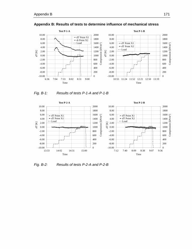
Appendix B 171
Appendix B: Results of tests to determine influence of mechanical stress
Fig. B-1: Results of tests P-1-A and P-1-B
Fig. B-2: Results of tests P-2-A and P-2-B
0
200
400
600
800
1000
1200
1400
1600
1800
2000
-10.00
-8.00
-6.00
-4.00
-2.00
0.00
2.00
4.00
6.00
8.00
10.00
6:36 7:04 7:33 8:02 8:31 9:00
dT Point X1dt Point X2Load
Test P-1-A Test P-1-B
Time Time
dT
[K]
dT
[K]
Com
pre
ssio
n[k
N/m
2]
Com
pre
ssio
n[k
N/m
2]
0
200
400
600
800
1000
1200
1400
1600
1800
2000
-10.00
-8.00
-6.00
-4.00
-2.00
0.00
2.00
4.00
6.00
8.00
10.00
10:55 11:24 11:52 12:21 12:50 13:19
dT Point X1
dT Point X2
Load
Test P-2-A Test P-2-B
Time Time
dT
[K]
dT
[K]
Com
pre
ssio
n[k
N/m
2]
Com
pre
ssio
n[k
N/m
2]
0
200
400
600
800
1000
1200
1400
1600
1800
2000
-10.00
-8.00
-6.00
-4.00
-2.00
0.00
2.00
4.00
6.00
8.00
10.00
13:33 14:02 14:31 15:00
dT Point X1dT Point X1Load
0
200
400
600
800
1000
1200
1400
1600
1800
2000
-10.00
-8.00
-6.00
-4.00
-2.00
0.00
2.00
4.00
6.00
8.00
10.00
7:12 7:40 8:09 8:38 9:07 9:36
dT Point X1dT Point X2Load
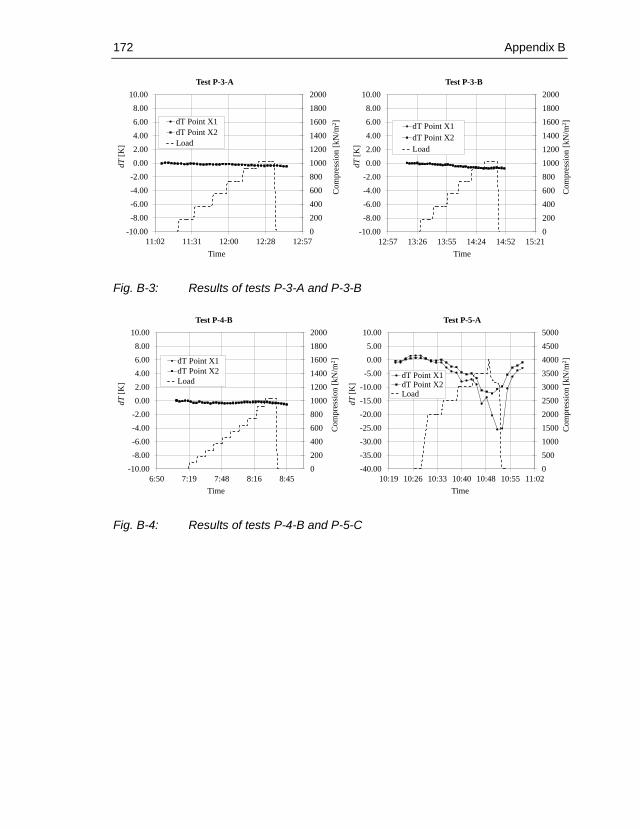
172 Appendix B
Fig. B-3: Results of tests P-3-A and P-3-B
Fig. B-4: Results of tests P-4-B and P-5-C
Test P-3-A Test P-3-B
Time Time
dT
[K]
dT
[K]
Com
pre
ssio
n[k
N/m
2]
Com
pre
ssio
n[k
N/m
2]
0
200
400
600
800
1000
1200
1400
1600
1800
2000
-10.00
-8.00
-6.00
-4.00
-2.00
0.00
2.00
4.00
6.00
8.00
10.00
12:57 13:26 13:55 14:24 14:52 15:21
dT Point X1
dT Point X2
Load
0
200
400
600
800
1000
1200
1400
1600
1800
2000
-10.00
-8.00
-6.00
-4.00
-2.00
0.00
2.00
4.00
6.00
8.00
10.00
11:02 11:31 12:00 12:28 12:57
dT Point X1
dT Point X2
Load
Test P-4-B Test P-5-A
Time Time
dT
[K
]
dT
[K]
Com
pre
ssio
n[k
N/m
2]
Com
pre
ssio
n[k
N/m
2]
0
200
400
600
800
1000
1200
1400
1600
1800
2000
-10.00
-8.00
-6.00
-4.00
-2.00
0.00
2.00
4.00
6.00
8.00
10.00
6:50 7:19 7:48 8:16 8:45
dT Point X1
dT Point X2
Load
0
500
1000
1500
2000
2500
3000
3500
4000
4500
5000
-40.00
-35.00
-30.00
-25.00
-20.00
-15.00
-10.00
-5.00
0.00
5.00
10.00
10:19 10:26 10:33 10:40 10:48 10:55 11:02
dT Point X1dT Point X2Load
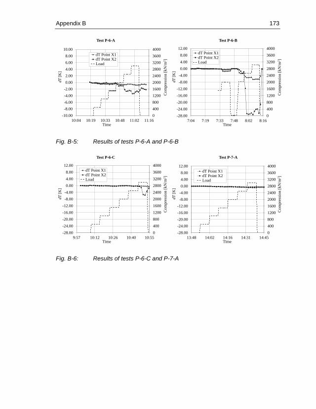
Appendix B 173
Fig. B-5: Results of tests P-6-A and P-6-B
Fig. B-6: Results of tests P-6-C and P-7-A
Test P-6-A Test P-6-B
Time Time
dT
[K]
dT
[K]
Com
pre
ssio
n[k
N/m
2]
Com
pre
ssio
n[k
N/m
2]
0
400
800
1200
1600
2000
2400
2800
3200
3600
4000
-10.00
-8.00
-6.00
-4.00
-2.00
0.00
2.00
4.00
6.00
8.00
10.00
10:04 10:19 10:33 10:48 11:02 11:16
dT Point X1dT Point X2Load
0
400
800
1200
1600
2000
2400
2800
3200
3600
4000
-28.00
-24.00
-20.00
-16.00
-12.00
-8.00
-4.00
0.00
4.00
8.00
12.00
7:04 7:19 7:33 7:48 8:02 8:16
dT Point X1dT Point X2Load
Test P-6-C Test P-7-A
Time Time
dT
[K]
dT
[K]
Com
pre
ssio
n[k
N/m
2]
Com
pre
ssio
n[k
N/m
2]
0
400
800
1200
1600
2000
2400
2800
3200
3600
4000
-28.00
-24.00
-20.00
-16.00
-12.00
-8.00
-4.00
0.00
4.00
8.00
12.00
9:57 10:12 10:26 10:40 10:55
dT Point X1dT Point X2Load
0
400
800
1200
1600
2000
2400
2800
3200
3600
4000
-28.00
-24.00
-20.00
-16.00
-12.00
-8.00
-4.00
0.00
4.00
8.00
12.00
13:48 14:02 14:16 14:31 14:45
dT Point X1dT Point X2Load

174 Appendix B
Fig. B-7: Results of tests P-7-B and P-8-A
Fig. B-8: Results of tests P-8-B and P-8-C
Test P-7-B Test P-8-A
Time Time
dT
[K]
dT
[K]
Com
pre
ssio
n[k
N/m
2]
Com
pre
ssio
n[k
N/m
2]
0
400
800
1200
1600
2000
2400
2800
3200
3600
4000
-28.00
-24.00
-20.00
-16.00
-12.00
-8.00
-4.00
0.00
4.00
8.00
12.00
6:57 7:12 7:26 7:40 7:55 8:09 8:24
dT Point X1dT Point X2Load
0
400
800
1200
1600
2000
2400
2800
3200
3600
4000
-28.00
-24.00
-20.00
-16.00
-12.00
-8.00
-4.00
0.00
4.00
8.00
12.00
11:24 11:52 12:21 12:50
dT Point X1dT Point X2Load
Test P-8-B Test P-8-C
Time Time
dT
[K]
dT
[K]
Com
pre
ssio
n[k
N/m
2]
Com
pre
ssio
n[k
N/m
2]
0
400
800
1200
1600
2000
2400
2800
3200
3600
4000
-28.00
-24.00
-20.00
-16.00
-12.00
-8.00
-4.00
0.00
4.00
8.00
12.00
9:14 9:28 9:43 9:57 10:12
dT Point X1dT Point X2Load
0
400
800
1200
1600
2000
2400
2800
3200
3600
4000
-28.00
-24.00
-20.00
-16.00
-12.00
-8.00
-4.00
0.00
4.00
8.00
12.00
13:48 14:02 14:16 14:31 14:45
dT Point X1dT Point X2Load

Appendix B 175
Fig. B-9: Results of tests P-9-A and P-9-B
Fig. B-10: Results of tests P-9-B and P-10-A
Test P-9-A Test P-9-B
Time Time
dT
[K]
dT
[K]
Com
pre
ssio
n[k
N/m
2]
Com
pre
ssio
n[k
N/m
2]
0
400
800
1200
1600
2000
2400
2800
3200
3600
4000
-28.00
-24.00
-20.00
-16.00
-12.00
-8.00
-4.00
0.00
4.00
8.00
12.00
12:50 13:04 13:19 13:33 13:48 14:02
dT Point X1dT Point X2Load
0
400
800
1200
1600
2000
2400
2800
3200
3600
4000
-28.00
-24.00
-20.00
-16.00
-12.00
-8.00
-4.00
0.00
4.00
8.00
12.00
10:12 10:26 10:40 10:55 11:09
dT Point X1dT Point X2Load
Test P-9-C Test P-10-A
Time Time
dT
[K]
dT
[K]
Com
pre
ssio
n[k
N/m
2]
Com
pre
ssio
n[k
N/m
2]
0
400
800
1200
1600
2000
2400
2800
3200
3600
4000
-28.00
-24.00
-20.00
-16.00
-12.00
-8.00
-4.00
0.00
4.00
8.00
12.00
7:48 8:16 8:45 9:14
dT Point X1dT Point X2Load
0
400
800
1200
1600
2000
2400
2800
3200
3600
4000
-28.00
-24.00
-20.00
-16.00
-12.00
-8.00
-4.00
0.00
4.00
8.00
12.00
8:45 9:00 9:14 9:28 9:43 9:57
dT Point X2dT Point X1Load
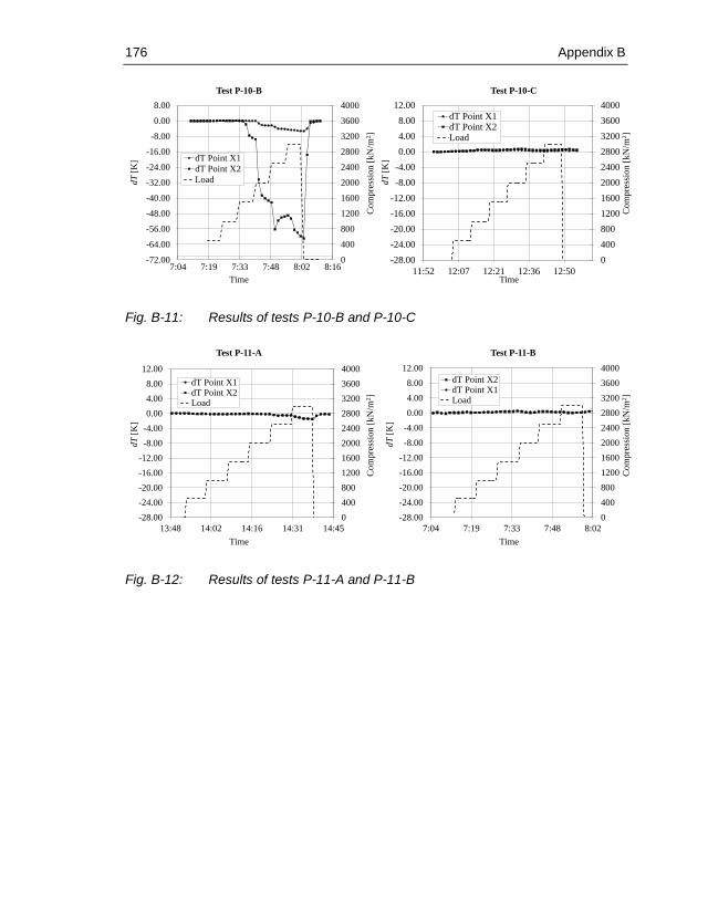
176 Appendix B
Fig. B-11: Results of tests P-10-B and P-10-C
Fig. B-12: Results of tests P-11-A and P-11-B
0
400
800
1200
1600
2000
2400
2800
3200
3600
4000
-28.00
-24.00
-20.00
-16.00
-12.00
-8.00
-4.00
0.00
4.00
8.00
12.00
11:52 12:07 12:21 12:36 12:50
dT Point X1dT Point X2Load
Test P-10-B Test P-10-C
Time Time
dT
[K]
dT
[K
]
Com
pre
ssio
n[k
N/m
2]
Com
pre
ssio
n[k
N/m
2]
0
400
800
1200
1600
2000
2400
2800
3200
3600
4000
-72.00
-64.00
-56.00
-48.00
-40.00
-32.00
-24.00
-16.00
-8.00
0.00
8.00
7:04 7:19 7:33 7:48 8:02 8:16
dT Point X1
dT Point X2
Load
Test P-11-A Test P-11-B
Time Time
dT
[K]
dT
[K]
Com
pre
ssio
n[k
N/m
2]
Com
pre
ssio
n[k
N/m
2]
0
400
800
1200
1600
2000
2400
2800
3200
3600
4000
-28.00
-24.00
-20.00
-16.00
-12.00
-8.00
-4.00
0.00
4.00
8.00
12.00
13:48 14:02 14:16 14:31 14:45
dT Point X1dT Point X2Load
0
400
800
1200
1600
2000
2400
2800
3200
3600
4000
-28.00
-24.00
-20.00
-16.00
-12.00
-8.00
-4.00
0.00
4.00
8.00
12.00
7:04 7:19 7:33 7:48 8:02
dT Point X2dT Point X1Load

Appendix B 177
Fig. B-13: Results of tests P-11-C
Test P-11-C
Time
dT
[K]
Co
mp
ress
ion
[kN
/m2]
0
400
800
1200
1600
2000
2400
2800
3200
3600
4000
-28.00
-24.00
-20.00
-16.00
-12.00
-8.00
-4.00
0.00
4.00
8.00
12.00
8:45 9:00 9:14 9:28 9:43 9:57
dT Point X1dT Point X2Load

178 Appendix B

Appendix C 179
Appendix C: Data sheets of investigated strain cables
Sensornet Damsense cableTM
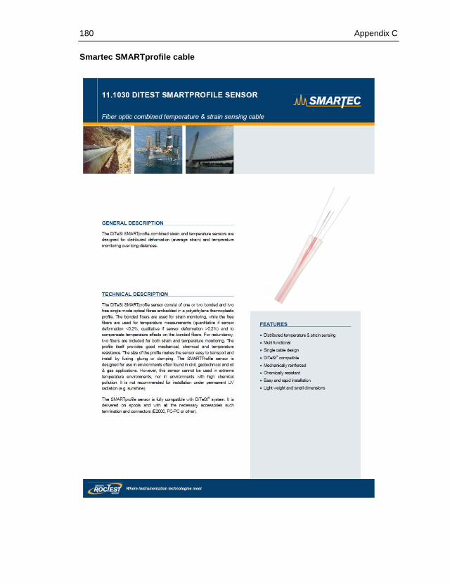
180 Appendix C
Smartec SMARTprofile cable

Appendix C 181

182 Appendix C
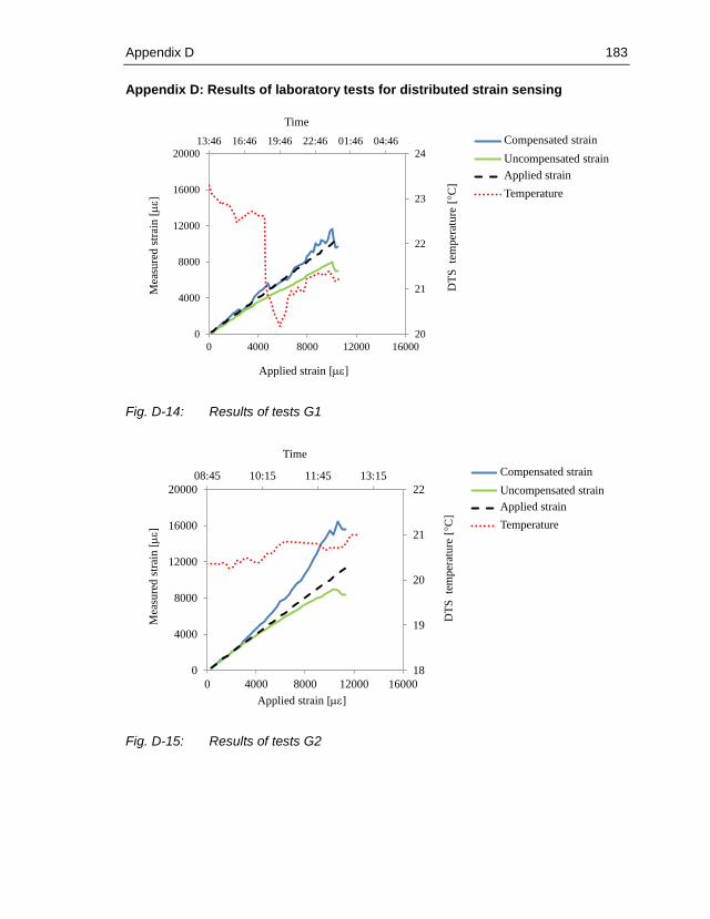
Appendix D 183
Appendix D: Results of laboratory tests for distributed strain sensing
Fig. D-14: Results of tests G1
Fig. D-15: Results of tests G2
Time
DT
S
tem
per
atu
re [ C
]
Mea
sure
d s
trai
n []
Applied strain []
Compensated strain
Uncompensated strain
Applied strain
Temperature
13:46 16:46 19:46 22:46 01:46 04:46
20
21
22
23
24
0
4000
8000
12000
16000
20000
0 4000 8000 12000 16000
time
DT
S -
tem
per
atu
re [ C
]
mea
sure
d s
tra
in [
me]
applied strain [me]
compensated
uncompensated
ideal
Temperatur
13:46 16:46 19:46 22:46 01:46 04:46
20
21
22
23
24
0
4000
8000
12000
16000
20000
0 4000 8000 12000 16000
time
DT
S -
tem
per
atu
re [ C
]
mea
sure
d s
tra
in [
me]
applied strain [me]
compensated
uncompensated
ideal
Temperatur
TimeD
TS
te
mp
erat
ure
[ C
]
Mea
sure
d s
trai
n []
Applied strain []
Compensated strain
Uncompensated strain
Applied strain
Temperature
13:46 16:46 19:46 22:46 01:46 04:46
20
21
22
23
24
0
4000
8000
12000
16000
20000
0 4000 8000 12000 16000
timeD
TS
-te
mp
era
ture
[ C
]
mea
sure
d s
tra
in [
me]
applied strain [me]
compensated
uncompensated
ideal
Temperatur
08:45 10:15 11:45 13:15
18
19
20
21
22
0
4000
8000
12000
16000
20000
0 4000 8000 12000 16000
time
DT
S -
tem
per
atu
re [ C
]
mea
sure
d s
train
[m
e]
applied strain [me]
compensated
uncompensate
d
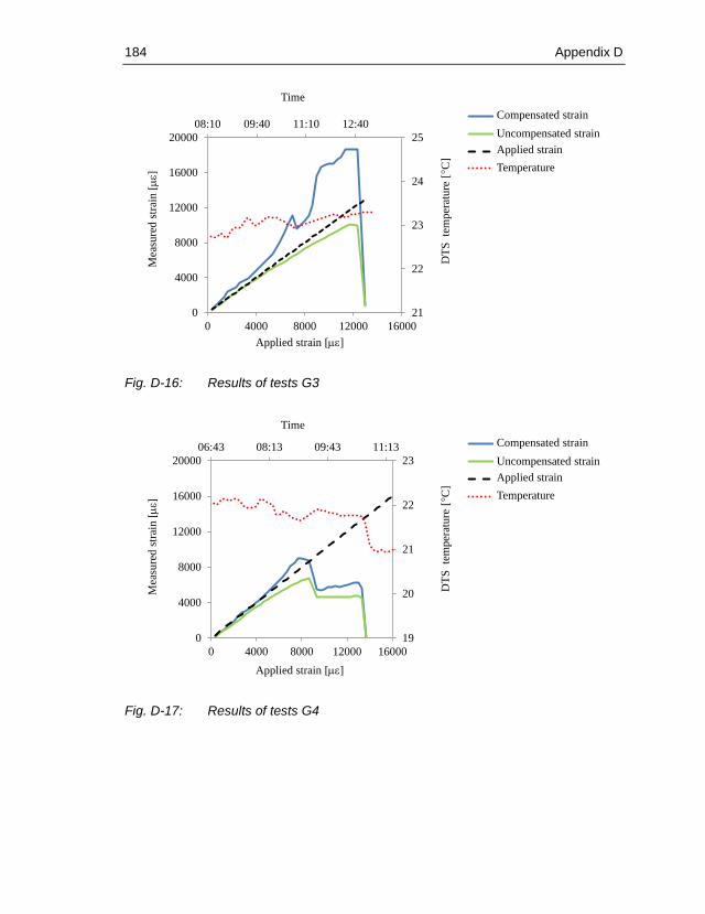
184 Appendix D
Fig. D-16: Results of tests G3
Fig. D-17: Results of tests G4
Time
DT
S
tem
per
atu
re [ C
]
Mea
sure
d s
trai
n []
Applied strain []
Compensated strain
Uncompensated strain
Applied strain
Temperature
13:46 16:46 19:46 22:46 01:46 04:46
20
21
22
23
24
0
4000
8000
12000
16000
20000
0 4000 8000 12000 16000
time
DT
S -
tem
per
atu
re [ C
]
mea
sure
d s
tra
in [
me]
applied strain [me]
compensated
uncompensated
ideal
Temperatur
08:10 09:40 11:10 12:40
21
22
23
24
25
0
4000
8000
12000
16000
20000
0 4000 8000 12000 16000
time
DT
S -
tem
per
atu
re [ C
]
mea
sure
d s
train
[m
e]
applied strain [me]
compensated
uncompensated
applied
Temperatur
Time
DT
S
tem
per
atu
re [ C
]
Mea
sure
d s
trai
n []
Applied strain []
Compensated strain
Uncompensated strain
Applied strain
Temperature
13:46 16:46 19:46 22:46 01:46 04:46
20
21
22
23
24
0
4000
8000
12000
16000
20000
0 4000 8000 12000 16000
time
DT
S -
tem
per
atu
re [ C
]
mea
sure
d s
tra
in [
me]
applied strain [me]
compensated
uncompensated
ideal
Temperatur
06:43 08:13 09:43 11:13
19
20
21
22
23
0
4000
8000
12000
16000
20000
0 4000 8000 12000 16000
timeD
TS
-te
mp
era
ture
[ C
]
mea
sure
d s
tra
in [
me]
applied strain [me]
compensated
uncompensated
applied
temperatur

Appendix D 185
Fig. D-18: Results of tests G5
Fig. D-19: Results of tests G6
Time
DT
S
tem
per
atu
re [ C
]
Mea
sure
d s
trai
n []
Applied strain []
Compensated strain
Uncompensated strain
Applied strain
Temperature
13:46 16:46 19:46 22:46 01:46 04:46
20
21
22
23
24
0
4000
8000
12000
16000
20000
0 4000 8000 12000 16000
time
DT
S -
tem
per
atu
re [ C
]
mea
sure
d s
tra
in [
me]
applied strain [me]
compensated
uncompensated
ideal
Temperatur
12:13 13:43 15:13 16:43
18
19
20
21
22
0
4000
8000
12000
16000
20000
0 4000 8000 12000 16000
time
DT
S -
tem
per
atu
re [ C
]
mea
sure
d s
train
[m
e]
applied strain [me]
compensated
uncompensated
applied
temperatur
Time
DT
S
tem
per
atu
re [ C
]
Mea
sure
d s
trai
n []
Applied strain []
Compensated strain
Uncompensated strain
Applied strain
Temperature
13:46 16:46 19:46 22:46 01:46 04:46
20
21
22
23
24
0
4000
8000
12000
16000
20000
0 4000 8000 12000 16000
time
DT
S -
tem
per
atu
re [ C
]
mea
sure
d s
tra
in [
me]
applied strain [me]
compensated
uncompensated
ideal
Temperatur
07:45 09:15 10:45 12:15
18
19
20
21
22
0
4000
8000
12000
16000
20000
0 4000 8000 12000 16000
timeD
TS
-te
mp
era
ture
[ C
]
mea
sure
d s
tra
in [
me]
applied strain [me]
compensated
uncompensated
applied
temperature

186 Appendix D
Fig. D-20: Results of tests G7
Fig. D-21: Results of tests G8
Mea
sure
d s
trai
n []
Applied strain []
Compensated strain
Uncompensated strain
Applied strain
0
4000
8000
12000
16000
20000
0 4000 8000 12000 16000
mea
sure
d s
train
[m
e]
applied strain [me]
compensated
uncompensated
applied
0
4000
8000
12000
16000
20000
0 4000 8000 12000 16000
mea
sure
d s
tra
in [
me]
applied strain [me]
compensated
uncompensated
applied
Mea
sure
d s
trai
n []
Applied strain []
Compensated strain
Uncompensated strain
Applied strain

Appendix D 187
Fig. D-22: Results of tests G9
Fig. D-23: Results of tests G10
Mea
sure
d s
trai
n []
Applied strain []
Compensated strain
Uncompensated strain
Applied strain
0
4000
8000
12000
16000
20000
0 4000 8000 12000 16000
mea
sure
d s
train
[m
e]
applied strain [me]
compensated
uncompensated
appliedM
easu
red s
trai
n []
Applied strain []
Compensated strain
Uncompensated strain
Applied strain
0
4000
8000
12000
16000
20000
0 4000 8000 12000 16000
mea
sure
d s
tra
in [
me]
applied strain [me]
compensated
uncompensated
applied
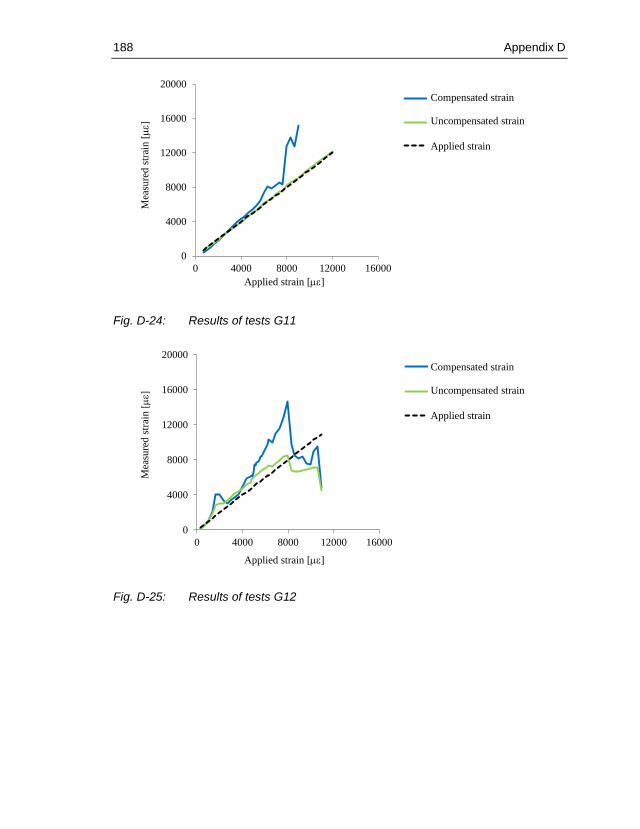
188 Appendix D
Fig. D-24: Results of tests G11
Fig. D-25: Results of tests G12
Mea
sure
d s
trai
n []
Applied strain []
Compensated strain
Uncompensated strain
Applied strain
0
4000
8000
12000
16000
20000
0 4000 8000 12000 16000
mea
sure
d s
tra
in [
me]
applied strain [me]
compensated
uncompensated
appliedM
easu
red
str
ain
[]
Applied strain []
Compensated strain
Uncompensated strain
Applied strain
0
4000
8000
12000
16000
20000
0 4000 8000 12000 16000
mea
sure
d s
train
[m
e]
applied strain [me]
compensated
uncompensated
ideal
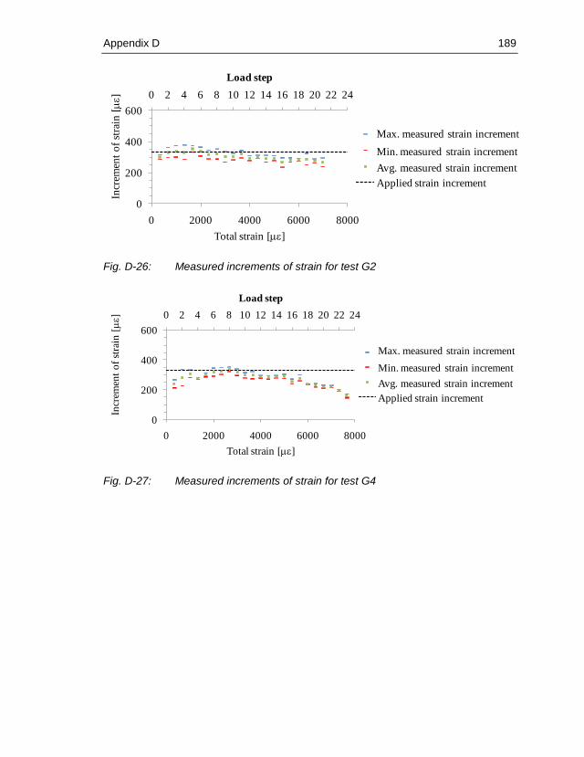
Appendix D 189
Fig. D-26: Measured increments of strain for test G2
Fig. D-27: Measured increments of strain for test G4
0 2 4 6 8 10 12 14 16 18 20 22 24
0
200
400
600
0 2000 4000 6000 8000
Load step
Incr
emen
t o
f st
rain
[]
Total strain []
Max.
Min
Aver.
Applied strain
Max. measured strain increment
Min. measured strain increment
Avg. measured strain increment
Applied strain increment
0 2 4 6 8 10 12 14 16 18 20 22 24
0
200
400
600
0 2000 4000 6000 8000
Load step
Incr
emen
t o
f st
rain
[]
Total strain []
Max.
Min
Aver.
Applied strain
Max. measured strain increment
Min. measured strain increment
Avg. measured strain increment
Applied strain increment
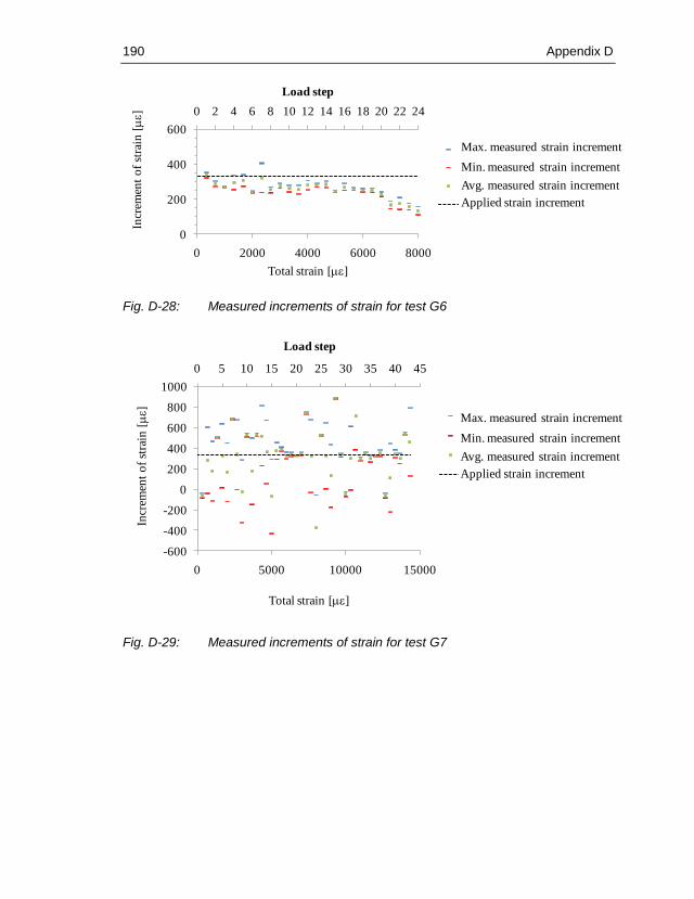
190 Appendix D
Fig. D-28: Measured increments of strain for test G6
Fig. D-29: Measured increments of strain for test G7
0 2 4 6 8 10 12 14 16 18 20 22 24
0
200
400
600
0 2000 4000 6000 8000
Load step
Incr
emen
t o
f st
rain
[]
Total strain []
Max.
Min
Aver.
Applied strain
Max. measured strain increment
Min. measured strain increment
Avg. measured strain increment
Applied strain increment
0 5 10 15 20 25 30 35 40 45
-600
-400
-200
0
200
400
600
800
1000
0 5000 10000 15000
Load step
Incr
emen
t o
f st
rain
[]
Total strain []
Max.
Min
Aver.
Applied strain
Max. measured strain increment
Min. measured strain increment
Avg. measured strain increment
Applied strain increment

Appendix D 191
Fig. D-30: Measured increments of strain for test G8
Fig. D-31: Measured increments of strain for test G9
0 5 10 15 20 25 30 35 40 45 50 55 60
-600
-400
-200
0
200
400
600
800
1000
0 5000 10000 15000 20000
Load step
Incr
emen
t o
f st
rain
[]
Total strain []
Max.
Min
Aver.
Applied strain
Max. measured strain increment
Min. measured strain increment
Avg. measured strain increment
Applied strain increment

192 Appendix D
Fig. D-32: Measured increments of strain for test G10
Fig. D-33: Measured increments of strain for test G11
0 5 10 15 20 25 30 35 40 45 50 55 60
-600
-400
-200
0
200
400
600
800
1000
0 5000 10000 15000 20000
Load step
Incr
emen
t o
f st
rain
[]
Total strain []
Max.
Min
Aver.
Applied strain
Max. measured strain increment
Min. measured strain increment
Avg. measured strain increment
Applied strain increment
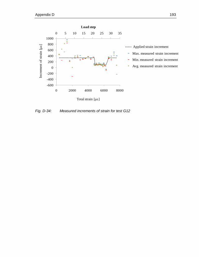
Appendix D 193
Fig. D-34: Measured increments of strain for test G12
0 5 10 15 20 25 30 35
-600
-400
-200
0
200
400
600
800
1000
0 2000 4000 6000 8000
Load step
Incr
emen
t o
f st
rain
[]
Total strain []
Applied strain
Max.
Min
Aver.
Max. measured strain increment
Min. measured strain increment
Avg. measured strain increment
Applied strain increment