Embed Size (px)
Citation preview

HAL Id: tel-01338604https://tel.archives-ouvertes.fr/tel-01338604
Submitted on 28 Jun 2016
HAL is a multi-disciplinary open accessarchive for the deposit and dissemination of sci-entific research documents, whether they are pub-lished or not. The documents may come fromteaching and research institutions in France orabroad, or from public or private research centers.
L’archive ouverte pluridisciplinaire HAL, estdestinée au dépôt et à la diffusion de documentsscientifiques de niveau recherche, publiés ou non,émanant des établissements d’enseignement et derecherche français ou étrangers, des laboratoirespublics ou privés.
A contribution to the theory of (signed) graphhomomorphism bound and Hamiltonicity
Qiang Sun
To cite this version:Qiang Sun. A contribution to the theory of (signed) graph homomorphism bound and Hamiltonicity.Information Theory [cs.IT]. Université Paris Saclay (COmUE), 2016. English. NNT : 2016SACLS109.tel-01338604

NNT : 2016SACLS109
THÈSE DE DOCTORATDE
L’UNIVERSITÉ PARIS-SACLAYPRÉPARÉE À
L’UNIVERSITÉ PARIS-SUD
LABORATOIRE DE RECHERCHE EN INFORMATIQUE
ECOLE DOCTORALE N° 580Sciences et technologies de l’information et de la communication
Spécialité Informatique
Par
M. Qiang Sun
A contribution to the theory of (signed) graphhomomorphism bound and Hamiltonicity
Thèse présentée et soutenue à Orsay, le 4 mai 2016 :
Composition du Jury :
Mme Kang, Liying Professeur, Shanghai University PrésidentM. Sopena, Éric Professeur, Université de Bordeaux RapporteurM. Woźniak, Mariusz Professeur, AGH University of Science and Technology RapporteurM. Manoussakis, Yannis Professeur, Université Paris-Sud ExaminateurM. Li, Hao Directeur de Recherche, CNRS Directeur de thèseM. Naserasr, Reza Chargé de Recherche, CNRS Co-directeur de thèse

“When things had been classified in organic categories,
knowledge moved toward fulfillness.”
Confucius (551-479 B.C.), The Great Learning
i

Acknowledgements
First of all, I would like to thank my supervisors Hao Li and Reza Naserasr for
giving me the opportunity to work with them.
I am grateful that Hao helped me a lot for administrative stuff when I applied my
PhD position here. I appreciate that he taught me how to find a research problem and
how to solve the problem when you find it. He is very nice to help me not only on works
but also on the things of life. I really appreciate his help.
I also would like to thank Reza. He taught me how to do research, how to write
papers, and how to give a presentation. I am grateful that he patiently explained things
that hard to understand in very detail.
I would like to thank Riste Skrekovski and Mirko Petrusevski. They invited me to
visit Slovenia and work with them.
I would like to thank Sagnik Sen. He gave me some good advices on doing PhD
when we worked together.
I would like to thank my colleagues in our lab. I hardly speak French, I am grateful
for their translations.
I would like to than some of my friends, Weihua Yang, Yandong Bai, Chuan Xu,
Meirun Chen, Jihong Yu and Weihua He, because of you my life in Paris is not boring.
I would also like to thank Beibei Wang for her advices on thesis writing, her en-
courage and support.
I am very grateful to my family for their understanding and support.
I am very grateful that China Scholarship Council supported my PhD study in
France.
Forgive me if I miss anyone. Thank you all.
ii

Abstract
In this thesis, we study two main problems in graph theory: homomorphism problem of
planar (signed) graphs and Hamiltonian cycle problems.
As an extension of the Four-Color Theorem, it is conjectured ([80], [41]) that every
planar consistent signed graph of unbalanced-girth d+1(d ≥ 2) admits a homomorphism
to signed projective cube SPC(d) of dimension d. It is naturally asked that:
Is SPC(d) an optimal bound of unbalanced-girth d + 1 for all planar consistent
signed graphs of unbalanced-girth d+ 1? (∗)
In Chapter 2, we prove that: if (B,Ω) is a consistent signed graph of unbalanced-
girth d which bounds the class of planar consistent signed graphs of unbalanced-girth
d, then |B| ≥ 2d−1. Furthermore, if no subgraph of (B,Ω) bounds the same class,
δ(B) ≥ d, and therefore, |E(B)| ≥ d · 2d−2. Our results showed that if the conjecture
([80], [41]) holds, then SPC(d) is an optimal bound both in terms of number of vertices
and number of edges.
When d = 2k, the problem (∗) is equivalent to the homomorphisms of graphs: is
PC(2k) an optimal bound of odd-girth 2k + 1 for P2k+1 (the class of all planar graphs
of odd-girth at least 2k + 1) ? Note that K4-minor free graphs are planar graphs, is
PC(2k) also an optimal bound of odd-girth 2k + 1 for all K4-minor free graphs of odd-
girth 2k+1 ? The answer is negative. In [6], a family of graphs of order O(k2) bounding
the K4-minor free graphs of odd-girth 2k + 1 were given. Is this an optimal bound? In
Chapter 3, we proved that: if B is a graph of odd-girth 2k + 1 which bounds all the
K4-minor free graphs of odd-girth 2k + 1, then |B| ≥ (k+1)(k+2)2 . Our result together
with the result in [6] shows that order O(k2) is optimal.
Furthermore, if PC(2k) bounds P2k+1, then PC(2k) also bounds P2r+1 (r > k).
However, in this case we believe that a proper subgraph of PC(2k) would suffice to
boundP2r+1, then what’s the optimal subgraph of PC(2k) that bounds P2r+1 ? The
first case of this problem which is not studied is k = 3 and r = 5. For this case, Naserasr
[81] conjectured that the Coxeter graph bounds P11. Supporting this conjecture, in
Chapter 4, we prove that the Coxeter graph bounds P17.
In Chapters 5, 6, we study the Hamiltonian cycle problems. Dirac showed in 1952
that every graph of order n is Hamiltonian if any vertex is of degree at least n2 . This
result started a new approach to develop sufficient conditions on degrees for a graph to
be Hamiltonian. Many results have been obtained in generalization of Dirac’s theorem.
In the results which strengthen Dirac’s theorem, there is an interesting research area: to
iii

control the placement of a set of vertices on a Hamiltonian cycle such that these vertices
have some certain distances among them on the Hamiltonian cycle.
In this thesis, we consider two related conjectures. One conjecture is given by
Enomoto: if G is a graph of order n ≥ 3 and δ(G) ≥ n2 + 1, then for any pair of vertices
x, y in G, there is a Hamiltonian cycle C of G such that distC(x, y) = bn2 c. Under the
same condition of this conjecture, it was proved in [32] that a pair of vertices are located
at distances no more than n6 on a Hamiltonian cycle. In [33], Faudree and Li studied
the case δ(G) ≥ n+k2 , 2 ≤ k ≤ n
2 . They proved that any pair of vertices can be located
at any given distance from 2 to k on a Hamiltonian cycle. Moreover, Faudree and Li
proposed a more general conjecture: if G is a graph of order n ≥ 3 and δ(G) ≥ n2 + 1,
then for any pair of vertices x, y in G and any integer 2 ≤ k ≤ n2 , there is a Hamiltonian
cycle C of G such that distC(x, y) = k.
Using Regularity Lemma and Blow-up Lemma, we gave a proof of Enomoto’s con-
jecture for graphs of sufficiently large order in Chapter 5, and gave a proof of Faudree-Li
conjecture for graphs of sufficiently large order in Chapter 6.
Keywords: signed graphs, projective cubes, homomorphism, walk-power, Hamil-
tonian cycle, Regularity Lemma.
iv

Resume
Dans cette these, nous etudions deux principaux problemes de la theorie des graphes: le
probleme d’homomorphisme des graphes planaires (signe) et celui du cycle Hamiltonien.
Generalisant le theoreme des quatre couleurs, il est conjecture ([80], [41]) que tout
graphe signe coherent planaire de maille-desequilibre d + 1(d ≥ 2) est homomorphe au
cube projectif signe SPC(d) de dimension d. On se demande naturallement:
SPC(d) est-elle une borne optimale de maille-desequilibre d+1 pour tous les graphes
signe coherent planaires de maille-desequilibre d+ 1?
Au Chapitre 2, nous prouvons que si (B,Ω) est un graphe signe coherent de maille-
desequilibre d qui borne la classe des graphes signes coherents planaires de maille-
desequilibre d + 1, alors |B| ≥ 2d−1. Par ailleurs, si aucun sous-graphe de (B,Ω) ne
borne la meme classe, alors le degre minimum de B est au moins d, et par consequent,
|E(B)| ≥ d · 2d−2. Notre resultat montre que si la conjecture ci-dessus est verifiee, alors
le cube SPC(d) est une borne optimale a la fois en termes des nombre de sommets et
de nombre des aretes.
Lorsque le d = 2k, le probleme est equivalent aux homomorphismes de graphe:
PC(2k) est-elle une borne optimale de maille-impair 2k + 1 pour P2k+2 (la classe de
tous graphes planaires de maille-impair au moins 2k + 1)? Observant que les graphes
K4-mineur libres sont les graphes planaires, PC(2k) est-elle aussi une borne optimale
de maille-impair 2k+ 1 pour tous les graphes K4-mineur libres de maille-impair 2k+ 1?
La reponse est negative, dans [6], une famille de graphes d’ordre O(k2) qui borne les
graphes K4-mineur libres de maille-impair 2k+1 est donnee. La borne est-elle optimale?
Au Chapitre 3, nous prouvons que si B est un graphe de maille-impair 2k+ 1 qui borne
tous les graphes K4-mineur libres de maille-impair 2k+ 1, alors |B| ≥ (k+1)(k+2)2 . Notre
resultat, avec que le resultat de [6] montre que l’ordre O(k2) est optimal.
En outre, si PC(2k) borne P2k+1, alors PC(2k) borne egalement P2r+1 (r > k).
Cependant, dans ce cas, nous croyons qu’un sous-graphe propre de PC(2k) suffirent a
borne P2r+1. Alors quel est le sous-graphe optimal de PC2k) qui borne P2r+1? Le
premier cas de ce probleme qui n’est pas etudiee est k = 3 et r = 5. Dans ce cas,
Naserasr [81] conjecture que le graphe Coxeter borne P11. Soutenir cette conjecture, au
Chapitre 4, nous prouvons que le graphe Coxeter borne P17.
Au Chapitres 5, 6, nous etudions les problemes du cycle hamiltonien. Dirac a
montre en 1952 que chaque graphe d’ordre n est Hamiltonien si tout sommet est de
degre au moins n2 . Ce resultat a commence une nouvelle approche pour developper
v

des conditions suffisantes sur degres pour caracteriser les graphes hamiltoniens. De
nombreux resultats ont ete obtenus generalisant le theoreme de Dirac. Parmi eux, il y a
une zone de recherche interessant: autour de la mise en place d’un ensemble de sommets
sur un cycle hamiltonien tel que ces sommets aient une certaine distance entre eux sur
ce cycle.
Dans cette these, nous considerons deux conjectures connexes, une proposir par
Enomoto: si G est un graphe d’ordre n ≥ 3 et δ(G) ≥ n2 + 1. Alors pour toute paire
de sommets x, y dans G, il y a un cycle hamiltonien C de G tel que distC(x, y) = bn2 c.Motive par cette conjecture, il a ete prouve, dans [32], qu’une paire de sommet ne peut
etre separee par une distance superievre a n6 sur un cycle hamiltonien. Dans [33], les
cas δ(G) ≥ n+k2 , 2 ≤ k ≤ n
2 , sont consideres, et il est prouve qu’une paire de sommets
a distance 2 a k peut etre pose sur un cycle hamiltonien. En outre, Faudree et Li ont
propose une conjecture plus generale: si G est un graphe d’ordre n ≥ 3 et δ(G) ≥ n2 + 1,
alors pour toute paire de sommets x, y dans G et tout entier 2 ≤ k ≤ n2 , il y a un
hamiltonien cycle C de G tel que distC(x, y) = k.
Utilisant le Lemme de Regularite et le Blow-up Lemma, dans le chapitre 5, nous
donnons une preuve de Enomoto conjecture pour les graphes d’ordre suffisant, et dans le
chapitre 6, nous donnons une preuve de la conjecture de Faudree et Li pour les graphes
d’order suffisant.
Mots-cles : graphes signe, cubes projectifs, homomorphisme, walk-power, cycle
hamiltonien, Regularity Lemma.
vi

Contents
Acknowledgements iv
Abstract v
Resume vii
List of Figures xiii
List of Tables xv
Symbols xvii
1 Introduction 1
1.1 Some background . . . . . . . . . . . . . . . . . . . . . . . . . . . . . . . . 1
1.1.1 Background of Part I . . . . . . . . . . . . . . . . . . . . . . . . . . 2
1.1.2 Background of Part II . . . . . . . . . . . . . . . . . . . . . . . . . 3
1.2 Basic terminology and notation . . . . . . . . . . . . . . . . . . . . . . . . 4
1.2.1 Terminology and notations of graphs . . . . . . . . . . . . . . . . . 4
1.2.2 Terminology and notations of signed graphs . . . . . . . . . . . . . 10
1.3 Motivations and overview . . . . . . . . . . . . . . . . . . . . . . . . . . . 12
1.3.1 Motivations and overview of Part I . . . . . . . . . . . . . . . . . . 12
1.3.2 Motivations and overview of Part II . . . . . . . . . . . . . . . . . 17
2 Cliques in walk-powers of planar graphs 27
2.1 Preliminaries . . . . . . . . . . . . . . . . . . . . . . . . . . . . . . . . . . 28
2.1.1 Planar graphs . . . . . . . . . . . . . . . . . . . . . . . . . . . . . . 28
2.1.2 Signed graphs . . . . . . . . . . . . . . . . . . . . . . . . . . . . . . 28
2.1.3 (Signed) projective cubes . . . . . . . . . . . . . . . . . . . . . . . 30
2.1.4 Walk-powers . . . . . . . . . . . . . . . . . . . . . . . . . . . . . . 32
2.2 Optimal bound for planar odd signed graphs . . . . . . . . . . . . . . . . 34
2.3 Optimal bound for planar signed bipartite graphs . . . . . . . . . . . . . . 40
2.4 Concluding remarks and further work . . . . . . . . . . . . . . . . . . . . 44
3 Cliques in walk-powers of K4-minor free graphs 45
3.1 K4-minor free graphs of odd-girth 2k + 1 . . . . . . . . . . . . . . . . . . 46
3.2 Proof of Theorem 3.2 . . . . . . . . . . . . . . . . . . . . . . . . . . . . . . 48
vii

Contents viii
3.3 Preliminaries for the proof of Theorem 3.3 . . . . . . . . . . . . . . . . . 50
3.4 Proof of Theorem 3.3 . . . . . . . . . . . . . . . . . . . . . . . . . . . . . . 54
3.4.1 G has a configuration in Figure 3.5 . . . . . . . . . . . . . . . . . . 55
3.4.2 G has a configuration in Figure 3.4 . . . . . . . . . . . . . . . . . . 55
3.5 Other cases of Conjecture 3.1 . . . . . . . . . . . . . . . . . . . . . . . . . 57
3.6 Concluding remarks and further work . . . . . . . . . . . . . . . . . . . . 59
4 Homomorphism and planar graphs 61
4.1 Kneser graphs and Coxeter graph . . . . . . . . . . . . . . . . . . . . . . . 62
4.2 Folding lemma and Euler formula . . . . . . . . . . . . . . . . . . . . . . . 66
4.3 Reducible configurations . . . . . . . . . . . . . . . . . . . . . . . . . . . . 67
4.4 Discharging and further reducible configurations . . . . . . . . . . . . . . 77
4.4.1 First phase of discharging . . . . . . . . . . . . . . . . . . . . . . . 78
4.4.2 Second phase of discharging . . . . . . . . . . . . . . . . . . . . . . 79
4.5 Concluding remarks and further work . . . . . . . . . . . . . . . . . . . . 84
5 Locating any two vertices on Hamiltonian cycles 85
5.1 Regularity Lemma and Blow-up Lemma . . . . . . . . . . . . . . . . . . . 85
5.1.1 Regular pairs and related properties . . . . . . . . . . . . . . . . . 86
5.1.2 Regularity Lemma and Blow-up Lemma . . . . . . . . . . . . . . . 87
5.1.3 Some applications of Regularity Lemma . . . . . . . . . . . . . . . 90
5.2 Overview of the proof of Theorem 5.2 . . . . . . . . . . . . . . . . . . . . 91
5.3 Non-extremal case . . . . . . . . . . . . . . . . . . . . . . . . . . . . . . . 93
5.3.1 Applying the Regularity Lemma . . . . . . . . . . . . . . . . . . . 93
5.3.2 Constructing paths to connect clusters . . . . . . . . . . . . . . . . 95
5.3.3 Handling of all the vertices of V0 . . . . . . . . . . . . . . . . . . . 100
5.3.4 Constructing the desired Hamiltonian cycle . . . . . . . . . . . . . 101
5.3.5 Other non-extremal cases . . . . . . . . . . . . . . . . . . . . . . . 103
5.4 Extremal cases . . . . . . . . . . . . . . . . . . . . . . . . . . . . . . . . . 105
5.4.1 Extremal case 1 . . . . . . . . . . . . . . . . . . . . . . . . . . . . . 105
5.4.2 Extremal case 2 . . . . . . . . . . . . . . . . . . . . . . . . . . . . . 111
5.5 Concluding remarks and further work . . . . . . . . . . . . . . . . . . . . 115
6 Distributing pairs of vertices on Hamiltonian cycles 117
6.1 Introduction . . . . . . . . . . . . . . . . . . . . . . . . . . . . . . . . . . . 117
6.2 Outline of the proof . . . . . . . . . . . . . . . . . . . . . . . . . . . . . . 118
6.3 Non-extremal case . . . . . . . . . . . . . . . . . . . . . . . . . . . . . . . 119
6.3.1 The graph order n is even . . . . . . . . . . . . . . . . . . . . . . . 119
6.3.2 The graph order n is odd . . . . . . . . . . . . . . . . . . . . . . . 125
6.4 Extremal cases . . . . . . . . . . . . . . . . . . . . . . . . . . . . . . . . . 126
6.4.1 Extremal case 1 . . . . . . . . . . . . . . . . . . . . . . . . . . . . . 126
6.4.1.1 The graph order n is even . . . . . . . . . . . . . . . . . . 126
6.4.1.2 The graph order n is odd . . . . . . . . . . . . . . . . . . 129
6.4.2 Extremal case 2 . . . . . . . . . . . . . . . . . . . . . . . . . . . . . 130
6.4.2.1 The graph order n is even . . . . . . . . . . . . . . . . . . 130
6.4.2.2 The graph order n is odd . . . . . . . . . . . . . . . . . . 133
6.5 Concluding remarks and further work . . . . . . . . . . . . . . . . . . . . 134

Contents ix
Bibliography 135
Publication 143

List of Figures
2.1 (a) A subdivision of K5, (b) a subdivision of K3,3 . . . . . . . . . . . . . . 28
2.2 An example of two equivalent signed graphs . . . . . . . . . . . . . . . . . 29
2.3 Copy and shortening of a thread. . . . . . . . . . . . . . . . . . . . . . . . 37
2.4 Example of building a planar graph G3 of odd-girth 5 with ω(G(3)3 ) ≥ 24. 39
3.1 Configuration 1 . . . . . . . . . . . . . . . . . . . . . . . . . . . . . . . . . 47
3.2 Configuration 2 . . . . . . . . . . . . . . . . . . . . . . . . . . . . . . . . . 47
3.3 Constructing aK4-minor free graphG of odd-girth 2k+1 with ω(G(2k−1)) ≥(k+1)(k+2)
2 . . . . . . . . . . . . . . . . . . . . . . . . . . . . . . . . . . . . . 48
3.4 Configuration 3 . . . . . . . . . . . . . . . . . . . . . . . . . . . . . . . . . 55
3.5 Configuration 4 . . . . . . . . . . . . . . . . . . . . . . . . . . . . . . . . . 55
4.1 Fano plane . . . . . . . . . . . . . . . . . . . . . . . . . . . . . . . . . . . 63
4.2 A representation of the Coxeter graph . . . . . . . . . . . . . . . . . . . . 64
4.3 Reducible configurations of adjacent 3-vertices with a Cox-coloring of theboundary. . . . . . . . . . . . . . . . . . . . . . . . . . . . . . . . . . . . . 73
4.4 Reducible configuration with a Cox-coloring of the boundary. . . . . . . . 74
4.5 Configuration F1 with a Cox-coloring of the boundary. . . . . . . . . . . . 75
4.6 Configuration F2 with a Cox-coloring of the boundary. . . . . . . . . . . . 76
4.7 Local configurations of a center of T014 supporting two poor vertices. . . . 82
4.8 Local configurations of a center of T023 supporting two poor vertices. . . . 83
4.9 Local configuration of a center of T122 supporting three poor vertices. . . . 84
5.1 Construction of Pi’s and Qi’s. . . . . . . . . . . . . . . . . . . . . . . . . . 99
5.2 Extending Qi−1 and Qi when u, v have a chain of length two. . . . . . . . 101
5.3 Construction of the Hamiltonian cycle C . . . . . . . . . . . . . . . . . . . 102
5.4 Extremal case 1. . . . . . . . . . . . . . . . . . . . . . . . . . . . . . . . . 109
5.5 Extremal case 2. . . . . . . . . . . . . . . . . . . . . . . . . . . . . . . . . 114
6.1 Construction of the Hamiltonian cycle . . . . . . . . . . . . . . . . . . . . 124
6.2 Extremal case 1 . . . . . . . . . . . . . . . . . . . . . . . . . . . . . . . . . 129
6.3 Extremal case 2 . . . . . . . . . . . . . . . . . . . . . . . . . . . . . . . . . 132
x

List of Tables
1.1 Cases of Conjecture 1.9 . . . . . . . . . . . . . . . . . . . . . . . . . . . . 13
xi
Symbols
ω(G) clique number of G
χ(G) chromatic number of G
α(G) independence number of G
c(G) circumference of G
δ(G) minimum degree of G
∆(G) maximum degree of G
(G)(r) r-th walk-power of G
G→ H G has a homomorphism to H
C ≺ H H bounds CPC(n) projective cube of dimension n
SPC(n) signed projective cube of dimension n
Forbm(H) the set of H-minor free graphs
xii
Chapter 1
Introduction
In 1736, Leonhard Euler gave a nice proof of a negative solution of well-known Seven
Bridges of Konigsberg problem. In his solution, he replaced each mass land with, in
modern term, an abstract vertex, and each bridge with an abstract connection, in modern
term, an edge. The resulting mathematical structure is called a graph now. Thus
Leonhard Euler laid the foundation of graph theory and his solution of Seven Bridges of
Konigsberg problem is considered as the first theorem of graph theory.
In this thesis, we will work on two topics in the graph theory: “Homomorphisms
of planar (signed) graphs to (signed) projective cubes”, which will be shown in Part I
(Chapter 2, 3, 4), and “Locating any two vertices on Hamiltonian cycles”, which will be
shown in Part II (Chapters 5, 6).
1.1 Some background
Around 1890, P. G. Tait concerned about the relationship between the existence of
Hamiltonian cycles and the Four-Colour Problem. The relationship is simply that if
a planar graph has a Hamiltonian cycle, then its faces can be 4-colored. Tait proved
that the Four-Colour Problem is equivalent to the problem of finding 3-edge-coloring of
bridgeless cubic planar graphs. Then Tait confined the attention on the cubic planar
graphs and conjectured that: Every bridgeless cubic planar graph has a Hamilton cycle.
Though this conjecture was disproved by W. T. Tutte in 1946, finding the extensions
of Four-Colour Problem and finding the Hamiltonian cycles in a given graph motivate
researchers a lot, these are the two main parts of this thesis.
1

Introduction 2
1.1.1 Background of Part I
The Four-Colour Theorem is one of the most notable theorem in graph theory, searching
a proof of it has motivated the development of graph theory a lot. The problem was
first proposed in 1852 by Francis Guthrie. The intuitive statement of the Four-Colour
Theorem was not in exact mathematical form, which is “ that given any separation of
a plane into contiguous regions, called a map, the regions can be colored using at most
four colors so that no two adjacent regions have the same color”. To put everything
in exact mathematical form, the set of regions can be represented abstractly as a set
of vertices, two vertices are connected by an edge if the two regions be represented are
adjacent. Thus the Four-Colour Theorem states, in graph-theoretic term, that “every
planar graph is 4-colorable”. In 1890, using Kempe chain method, Percy Heawood[50]
proved that “every planar graph is 5-colorable”. In 1976, Kenneth Appel and Wolfgang
Haken [3] proved the Four-Colour Theorem. In their proof, computer and program are
used.
The study of the Four-Colour Theorem led to the theory of vertex-coloring. Nat-
urally, many other kinds of graph colorings have been defined and studied, such as
edge-coloring, fractional coloring, acyclic coloring, etc.. Graph coloring came out to be
a fruitful branch of graph theory, even a notable branch of mathematics. During the
approach to The Four-Colour Theorem, it is generalized in many different ways: frac-
tional coloring, circular coloring, graph minors and, in particular, the theory of graph
homomorphisms, which is one of the main topics of this thesis.
In the language of graph minors, the Four-Colour Theorem states that: “Any graph
G which does not contain complete graph K5 or complete bipartite graph K3,3 as a minor
is 4-colorable”. As one of the most well-known conjectures that extend the Four-Colour
Theorem, Hadwiger’s conjecture was proposed by H. Hadwiger in 1943.
Conjecture 1.1 (Hadwiger). Any graph G which does not contain Kn as a minor is
(n− 1)-colorable.
In the language of graph homomorphisms, the Four-Colour Theorem states that:
“Every planar graph admits a homomorphism to the complete graph K4”. If the planar
graph is bipartite, it admits a homomorphism to complete graph K2. Thus we only
need to consider the non-bipartite planar graphs, i.e., planar graphs of odd-girth at
least 3. Note that K4 is isomorphic to PC(2) (projective cube of dimension 2, defined in
Section 1.2), in 2007, R. Naserasr proposed a conjecture which extends the Four-Colour
Theorem:
Conjecture 1.2 ([80]). Given an integer k ≥ 1, every planar graph of odd-girth at least
2k + 1 admits a homomorphism to PC(2k).

Introduction 3
Using the notation of signed graphs and SPC(k) (signed projective cubes of dimen-
sion k, defined in Section 1.2), the above conjecture was extended to include the planar
bipartite graphs, as introduced in [80] and [41]:
Conjecture 1.3. Given an integer k ≥ 2, every planar consistent signed graph of
unbalanced-girth k + 1 admits a homomorphism to SPC(k).
A lot of work has been done with respect to these two conjectures while a lot of
problems are left to be solved. The Part I of this thesis will focus on some related
problems.
1.1.2 Background of Part II
The Hamiltonian paths and Hamiltonian cycles are named after Sir William Rowan
Hamilton who invented the Icosian Game. In 1856, Hamilton invented a mathematical
game, the Icosian Game, which consists of a dodecahedron. Each vertex of the dodeca-
hedron is labled with the name of a city and the game’s object is finding a (Hamiltonian)
cycle along the edges of the dodecahedron such that every vertex is visited a single time,
and the ending point is the same as the starting point. Since then, the Hamiltonian
problem, determining when a graph contains a Hamiltonian cycle, has been fundamen-
tal in graph theory. In fact, as a generalization of Hamiltonian cycles, circumferences,
dominating cycles, pancyclic, cyclability etc. are well studied, and a huge number of
results have been produced by researchers.
Note that it is NP-complete to determine whether there exists a Hamiltonian cycle in
a graph, finding necessary or sufficient conditions for hamiltonicity become an interesting
topic in graph theory. Every complete graph on at least three vertices is evidently
Hamiltonian, indeed, to get a Hamiltonian cycle in a complete graph, we can start from
any vertex, and choose the vertices one by one in an arbitrary order. If a graph does
not have so many edges, how large of a minimum degree can guarantee the existence of
a Hamiltonian cycle? In 1952, G. A. Dirac[23] answered this question by showing that
if a simple graph has order at least 3 and each vertex has the degree at least half of the
order, then the graph is Hamiltonian. This original result started a new approach to
develop sufficient conditions on degrees for a graph to contain a Hamiltonian cycle.
There are plenty of results to strengthen Dirac’s theorem. One of the interesting
research areas is to control the placement of a set of vertices on the Hamiltonian cycle
such that these vertices have some certain distances among them on the Hamiltonian
cycle. Enomoto proposed the following conjecture of exact placement for a pair of
vertices at a precise distance (half of the graph order) on a Hamiltonian cycle.

Introduction 4
Conjecture 1.4 ([39]). If G is a graph of order n ≥ 3 and δ(G) ≥ n2 +1, then for any pair
of vertices x, y in G, there is a Hamiltonian cycle C of G such that distC(x, y) = bn2 c.
In 2012, Faudree and Li proposed a more general conjecture.
Conjecture 1.5 ([33]). If G is a graph of order n ≥ 3 and δ(G) ≥ n2 + 1, then for any
pair of vertices x, y in G and any integer 2 ≤ k ≤ n2 , there is a Hamiltonian cycle C of
G such that distC(x, y) = k.
The Part II of this thesis will focus on these two conjectures.
1.2 Basic terminology and notation
In this section we provide some basic terminology and notations for the rest of the thesis.
The definitions not given here will be mentioned in the beginning of the respective
chapters.
First, we give some basic terminology and notations of graph.
1.2.1 Terminology and notations of graphs
A graph G is an ordered pair (V (G), E(G)) with a set V (G) of vertices and a set E(G),
disjoint from V (G), of edges, together with an incidence function ψG that associates
with each edge of G an unordered pair of (not necessarily distinct) vertices of G. Given
an edge e, if ψG(e) = u, v, then e is said to join u and v; u and v are called the ends
of e; moreover, u and v are said to be adjacent. In this thesis, we write e = uv instead of
ψG(e) = u, v. A loop is an edge with identical ends. Two edges e1 and e2 (which are
not loops) are said to be parallel if they have the same pair of ends. A graph is simple
if it has neither loops nor parallel edges. A graph with parallel edges and without loops
is called a multigraph.
The order of a graph is the cardinality of its set of vertices and the size of a graph
is the cardinality of its set of edges. The order of a graph G is denoted by |V (G)| or |G|.
Subgraphs
A subgraph H = (V (H), E(H)) of a graph G is a graph with V (H) ⊆ V (G) and
E(H) ⊆ E(G). We write H ⊆ G if H is a subgraph of G.
Introduction 5
Given a nonempty subset V ′ of V (G), the subgraph with vertex set V ′ and edge set
uv ∈ E(G)|u, v ∈ V ′ is called the subgraph of G induced by V ′, denoted G[V ′]. We
say that G[V ′] is an induced subgraph of G.
Let F be a set of graphs. A graph is said to be F -free if it does not contain any
graph from the set F as a subgraph.
Disjoint union of graphs
Given two graphs G1 = (V1, E1) and G2 = (V2, E2) with V1∩V2 = ∅ and E1∩E2 = ∅,the disjoint union of G1 and G2, denoted G1 ∪G2, is the graph with vertex set V1 ∪ V2
and edge set E1 ∪ E2.
Complete join of graphs
Given two graphs G1 = (V1, E1) and G2 = (V2, E2) with V1∩V2 = ∅ and E1∩E2 = ∅,the complete join of G1 and G2, denoted G1 + G2, is the graph obtained by starting
with G1 ∪G2 and adding edges joining every vertex of G1 to every vertex of G2.
Walk, path and cycle
A walk in a graph G is a finite non-null sequence W := v0e1v1e2v2 . . . ekvk, whose
terms are alternately vertices and edges of G (not necessarily distinct), such that the
ends of ei(1 ≤ i ≤ k) are vi−1 and vi. We say that v0 and vk are connected by W . The
vertices v0 and vk are called the ends of W , v0 being its initial vertex and vk being its
terminal vertex ; the vertices v1, . . . , vk−1 are its internal vertices. A v0-walk is a walk
with initial vertex v0. The length of a walk is the number of its edge. A walk of length
k is also called a k-walk. If v0 = vk, we call W a closed walk.
If the vertices v0, v1, . . . , vk of W are distinct, W is called a path or v0-vk path.
If the vertices v0, v1, . . . , vk−1 of W are distinct and v0 = vk, W is called a cycle.
The length of a path or a cycle is the number of its edges. A path or a cycle of length
k is called a k-path or k-cycle, respectively; the path or cycle is odd or even according
to the parity of its length.
Hamiltonian cycle
In a graph G, a Hamiltonian cycle is a cycle that visits each vertex of G exactly
once. A graph that contains a Hamiltonian cycle is called a Hamiltonian graph.
Distance, diameter and neighbors

Introduction 6
The distance dG(x, y) of two vertices x, y in G is the length of a shortest x-y path
in G. Whenever the underlying graph is clear from the context, we will write d(x, y)
instead of dG(x, y).
The diameter of a connected graph G is the greatest distance between any two
vertices in G.
Given a positive integer i and a vertex x of G, Ni(x) denotes the set of i-th neighbors
of x, i.e., the set of vertices at distance exactly i from x. When i = 1, we simply write
N(x). For U ⊆ V (G) we write Ni(U) =⋃x∈U Ni(x).
Girth and circumference
The girth of a graph is the length of a shortest cycle contained in the graph. The
odd-girth of a graph is the length of a shortest odd-cycle contained in the graph. The
circumference of a graph G is the length of a longest cycle contained in G, denoted
c(G). If a graph does not contain any cycle, its girth and circumference are defined to
be infinity.
Complete graphs and cliques
A complete graph is a simple graph such that any two vertices are connected by an
edge. If a complete graph is of order n, we denote it by Kn.
A clique of a graph G is a complete graph contained in G as a subgraph. The clique
number ω(G) of a graph G is the order of a maximum clique in G.
Bipartite graphs
A graph is bipartite if its vertex set can be partitioned into two subsets V1 and V2
such that every edge has one end in V1 and the other end in V2. Equivalently, a graph
is bipartite if it does not contain any odd-cycle.
Planar graphs
A graph is planar if it can be drawn on the plan such that its edges intersect only
at their ends. Such a drawing is called a planar embedding of the graph. Given a
planar embedding of a planar graph, it divides the plan into a set of connected regions,
including an outer unbounded connected region. Each of these regions is called a face
of the planar graph. The boundary of a face is the cycle of the graph containing it. A
planar graph with a given planar embedding is called a plane graph. We denote the
class of planar graph of odd-girth at least 2k + 1 by P2k+1.
Degree and regularity

Introduction 7
In a simple graph G, for any vertex v of G, the degree of v is the number of vertices
adjacent to v in G. We will use dG(v) (or d(v) when there is no chance of confusion) to
denote the degree of v in Chapter 2,3,4, while in Chapter 5, 6 we use degG(v) or deg(v).
A d-regular graph is a graph in which every vertex has degree d. A 3-regular graph is
also known as a cubic graph.
Cayley graphs
Let Γ be a group, S be a set of elements of Γ not including the identity element.
Suppose, furthermore, that the inverse of every element of S also belongs to S. The
Cayley graph C(Γ, S) is the graph with vertex set Γ in which two vertices x and y are
adjacent if and only if xy−1 ∈ S.
Hypercubes
The hypercube of dimension n, denoted H(n), is the graph whose vertex set is
the set all n-tuples of 0’s and 1’s, where two n-tuples are adjacent if and only if they
differ in precisely one coordinate. It can be checked that, H(n) is a Cayley graph
(Zn2 , e1, e2, . . . , en) where ei’s are the standard basis of Zn2 . H(n) is also called n-cube.
Projective cubes
The Projective cube of dimension n, denoted PC(n), is the graph obtained by iden-
tifying the antipodal vertices of the hypercube H(n+1), or equivalently, by adding edges
between pairs of antipodal vertices of the hypercube H(n). PC(n) can be represented
as a Cayley graph, that is, PC(n) = (Zn2 , e1, e2, . . . , en, J) where ei’s are the standard
basis of Zn2 and J is the all 1 vector of relevant length (n here). Projective cubes are
also known as folded cubes.
Kneser graph K(n, k)
Given positive integers n and k such that n ≥ 2k, the Kneser graph K(n, k) is
defined to be the graph whose vertices correspond to the k-element subsets of a set of n
elements, where two vertices are adjacent if the two corresponding sets are disjoint.
Minors
In a graph G, an edge contraction is an operation which removes an edge and
identify the vertices of the edge. A graph H is called a minor of the graph G if H can
be obtained from G by a series of deleting edges, vertices and contracting edges. Given
a graph H, a graph is said to be H-minor free if it does not contain H as a minor. Let
H be a set of graphs. A graph is said to be H-minor free if it does not contain any
graph from H as a minor. Moreover, we use Forbm(H) to denote the class of all graphs
that have no member of H as a minor, that means the set of H-minor free graphs.

Introduction 8
Connectivity
A graph is connected if any pair of vertices is connected by a path. A connected
graph G is said to be k-vertex-connected (or k-connected) if it has more than k ver-
tices and remains connected whenever fewer than k vertices are removed. Similarly,
a connected graph G is said to be k-edge-connected if it remains connected whenever
fewer than k edges are removed. The vertex-connectivity (or just connectivity) (or edge-
connectivity, respectively), of a graph is the largest k for which the graph is k-vertex-
connected (or k-edge-connected, respectively). A bridge, or cut-edge, is an edge of a
graph whose deletion increases its number of components. A graph is bridgeless if it
contains no bridges, that means each component of it is 2-edge-connected.
k-tough graph
Let t(G) denote the number of components of a graph G. A graph G is k-tough
if kt(G − S) ≤ |S| for every subset S of the vertex set V (G) with t(G − S) > 1. The
toughness of G, denoted τ(G), is the maximum value of k for which G is k-tough (taking
τ(Kn) =∞ for all n ≥ 1).
Pancyclic and bipancyclic graphs
A graph G is called pancyclic if it contains cycles of all length k for 3 ≤ k ≤ |V (G)|.Analogously, a bipartite graph G is called bipancyclic if it contains cycles of all even
lengths from 4 to |V (G)|.
Independent set
An independent set of a graph G is a subset of the vertices such that no two vertices
in the subset induce an edge of G. The cardinality of a maximum independent set in a
graph G is called the independence number of G, denoted α(G).
Homomorphisms
Let G and H be two graphs. A homomorphism of G to H is a mapping ϕ : V (G)→V (H) such that ϕ(u)ϕ(v) ∈ E(H) whenever uv ∈ E(G). If G admits a homomorphism
to H, we write G→ H. We say that two graphs G and H are hom-equivalent if G→ H
and H → G.
The image of G under ϕ is called a homomorphic image of G. Given a class C of
graphs and a graph H, if every graph in C admits a homomorphism to H we write C Hand we say H bounds C. Given a finite set H of connected graphs, we use Forbh(H) to
denote the class of all graphs which do not admit a homomorphism from any member
of H.

Introduction 9
Isomorphisms
Let G and H be two graphs. An isomorphism between G and H is a bijection
ϕ : V (G) → V (H) such that ϕ(u)ϕ(v) ∈ E(H) if and only if uv ∈ E(G). Two graphs
are isomorphic if there exists an isomorphism between them.
Embedding
An embedding of a graph H into a graph G is an isomorphism between H and a
subgraph of G. We say H is embeddable into G if there exists an embedding of H into
G.
Vertex-coloring and edge-coloring
A k-vertex-coloring (or k-edge-coloring, respectively) of a graph G is a mapping:
c : V (G) → S (or c : E(G) → S, respectively), where S is a set of k colors, usually the
set S of colors is taken to be 1, 2, . . . , k. Thus a k-vertex-coloring (or k-edge-coloring,
respectively) is an assignment of k colors to the vertices (or edges, respectively) of G. A
vertex-coloring (or edge-coloring, respectively) c is proper if no two adjacent vertices (or
incident edges, respectively) are assigned a same color. A graph is k-vertex-colorable (or
k-edge-colorable, respectively) if it has a k-vertex-coloring (or k-edge-coloring, respec-
tively). The minimum k for which a graph G is k-vertex-colorable (or k-edge-colorable,
respectively) is called its chromatic number (or chromatic index, respectively).
Fractional coloring
Let I(G) denote the set of all independent vertex sets of a graph G, and let I(G, u)
denote the independent vertex sets of G that contain the vertex u. A fractional coloring
of G is a defined as a nonnegative real function f on I(G) such that for any vertex u of
G,∑
S∈I(G,u) f(S) ≥ 1. The sum of values of f is called its weight, and the minimum
possible weight of a fractional coloring is call the fractional chromatic number of G.
Circular coloring
Given a graph G and positive integers p and q and a color set C = 0, 1, . . . , p−1, if
there is a mapping c : V (G)→ C such that: for each edge uv ∈ E(G), q ≤ |c(u)−c(v)| ≤p− q, then we say G has a circular-pq -coloring, or G is circular-pq -colorable.
Walk-powers of graphs
Given a graph G and a positive integer k, we define the k-th walk-power of G,
denoted G(k), to be the graph whose vertex set is also V (G) with two vertices x and y
being adjacent if there is a walk of length k connecting x and y in G.
In the following, we give some basic terminology and notations of signed graphs.

Introduction 10
1.2.2 Terminology and notations of signed graphs
Signed graphs
Given a graph G, we assign a sign “+” or “−” to each edge of G. The edges labeled
“+” are called positive edges while the ones labeled “−” are called negative edges. We
can see this assignment as a mapping of the edges of G to the set +,−. Such a
mapping is called a signature of G. We normally denote the set of negative edges by Σ.
Note that, a signature of G is given if and only if the set of negative edges is given, thus
the set of edges Σ will be referred to as the signature of G, and (G,Σ) is called a signed
graph.
Resigning
Given a signed graph (G,Σ) and a vertex v ∈ V (G), a resigning at v is to change
the sign of each edge incident to v. Two signatures Σ1, Σ2 on a graph G are said to be
equivalent if one can be obtained from the other by a sequence of resignings, moreover,
(G,Σ1) and (G,Σ2) are also said to be equivalent. Thus resigning defines an equivalence
relations on the set of all signed graphs over a graph. Given a signed graph (G,Σ),
denote [G,Σ] the set of all signed graphs equivalent to (G,Σ).
Unbalanced-girth
In a signed graph (G,Σ), a cycle with an odd (or even, respectively) number of
negative edges is called unbalanced (or balanced, respectively). Note that resignings do
not change the balance of a cycle. Recall that an odd-cycle is a cycle of odd length while
a cycle of (G,E(G)) is unbalanced if and only if it is an odd-cycle of G, the notation
of unbalanced cycle is, in some sense, an extension of the notation of an odd-cycle.
Similar to the definition of odd-girth of G, we define the unbalanced-girth of (G,Σ) as
the shortest length of an unbalanced cycle of (G,Σ). A signed graph is balanced if all
its cycles are balanced.
Consistent signed graphs
A consistent signed graph is a signed graph in which every balanced cycle is of even
length and all unbalanced cycles are of the same parity. Thus there are two types of
consistent signed graphs:
i. when all unbalanced cycles are of odd length (it can be shown that this is the case
if and only if Σ ≡ E(G)), such a signed graph will be called an odd signed graph;

Introduction 11
ii. when all unbalanced cycles are of even length (which will be the case if and only
if G is bipartite), such a signed graph thus will be referred to as a signed bipartite
graph.
Signed projective cubes
The signed projective cube of dimension n, denoted SPC(n), is the signed graph
(PC(n),Σ), where Σ is the set of edges corresponding to J according to the definition
of PC(n). On the other hand, Σ can be viewed as the set of edges added between pairs
of antipodal vertices of hypercube Hn to get PC(n).
Homomorphisms of signed graphs
Given two signed graphs (G1,Σ1) and (G2,Σ2), we say that there is a homomor-
phism of (G1,Σ1) to (G2,Σ2) if there exist a signed graph (G,Σ′1) equivalent to (G1,Σ1),
a signed graph (G2,Σ′2) equivalent to (G2,Σ2) and a mapping ϕ : V (G1) → V (G2)
such that: ϕ(x)ϕ(y) ∈ E(G2) whenever xy ∈ E(G1) and xy ∈ Σ′1 if and only if
ϕ(x)ϕ(y) ∈ Σ′2. When there exists a homomorphism of (G1,Σ1) to (G2,Σ2), we write
(G1,Σ1) → (G2,Σ2). Given a class C of signed graphs, we say a signed graph (H,Σ)
bounds C if every member of C admits a homomorphism to (H,Σ).
Minors of signed graphs
A (signed) minor of a signed graph (G1,Σ1) is a signed graph (G2,Σ2) obtained
from (G1,Σ1) by a sequence of the following operations: (i) delete an edge (and remove
it from the signature if it is present), (ii) contract a positive edge (that means it is not
in the signature), (iii) resign at any vertex. These operations can be taken in any order.
We say that (G1,Σ1) is (G2,Σ2)-minor free if it does not contain (G2,Σ2) as a minor.
Cover and pack
Given a signed graph (G,Σ) and a set B of edges of (G,Σ), we call B an (unbalanced
cycle) cover if every unbalanced cycle of (G,Σ) contains at least one edge ofB. Moreover,
denote by τ(G,Σ) the unbalanced-girth of (G,Σ) and denote by ν(G,Σ) the maximum
number of pairwise disjoint covers of (G,Σ). Since every unbalanced cycle intersect
every cover, τ(G,Σ) ≥ ν(G,Σ). If τ(G,Σ) = ν(G,Σ), we say that (G,Σ) packs.

Introduction 12
1.3 Motivations and overview
1.3.1 Motivations and overview of Part I
The existence of a homomorphism from a class of graphs to a projective cube is of
special importance. Generally, Conjecture 1.2 and Conjecture 1.3 capture a certain
packing problem and edge-coloring problem.
A packing problem of signed graphs was introduced by Guenin [41]. In this paper,
Guenin proposed a conjecture which he called main conjecture:
Conjecture 1.6. [41] Consistent signed graphs which are (K5, E(K5))-minor free, pack.
Guenin pointed out that Conjecture 1.6 is a special case of a conjecture on binary
clutters in [93]. Using the Proposition 1.7 below, Guenin showed that the Four-Colour
Theorem is a special case of the Conjecture 1.6. Also it is proved that Conjecture 1.6
implies other conjectures, we will introduce this later.
Proposition 1.7. [41] Let (G,Σ) be a signed graph and let k be a positive integer.
Suppose k is even and G is bipartite or k is odd and Σ = E(G). Then the following
statements are equivalent,
(1) there exist k disjoint covers of (G,Σ),
(2) (G,Σ) is homomorphic to SPC(k − 1).
In [82], Naserasr, Rollova and Sopena independently Proposition 1.7. This propo-
sition shows that the problem of finding a mapping of a consistent signed graph to a
signed projective cube is equivalent to a packing problem.
The study of edge-coloring has a long history in graph theory, it has a close link
to the Four-Colour Theorem. Edge-coloring of graphs were first considered in two short
papers by Tait [97] published in the same proceeding between 1878 and 1880. Tait proved
a theorem relating face-coloring and edge-coloring of planar graphs. Tait’s theorem says
that if G is a bridgeless cubic planar (simple) graph, then G admits a 3-edge-coloring if
and only if the faces of G can be colored with four colors such that the adjacent faces
receive different colors. Thus Tait conjectured that every bridgeless 3-regular planar
graph admits a 3-edge-coloring. Since the conjecture is equivalent to the Four-Color
Theorem, we state Tait’s conjecture as a theorem.
Theorem 1.8. (Tait’s Conjecture [100]) Every bridgeless 3-regular planar graph is 3-
edge-colorable.

Introduction 13
In 1981, P.D. Seymour proposed a generalization to Tait’s conjecture, which use
the following notations.
Given a graph G, let X,Y be a partition of V (G) and let [X,Y ] denote the set of all
edges with one end in X and the other end in Y . Then [X,Y ] is said to be a cut of G.
Moreover, if |X| or |Y | is odd, we call [X,Y ] an odd cut of G. The size of a cut [X,Y ]
is |[X,Y ]|. An r-graph is an r-regular graph with no odd cut of size less than r.
Conjecture 1.9. ([95]) Every planar r-graph is r-edge-colorable.
It is proved that Conjecture 1.9 can be implied by Conjecture 1.6. The cases
3 ≤ r ≤ 8 of this conjecture are proved, as shown in the following table. In [80] Naserasr
Cases Proved by
r = 3 Tait [100]
r = 4, 5 Guenin [42]
r = 6 Dvorak, Kawarabayashi, Kral [24]
r = 7 Chudnovsky, Edwards, Kawarabayashi, Seymour [19]
r = 8 Chudnovsky, Edwards and Seymour [20]
r ≥ 9 open
Table 1.1: Cases of Conjecture 1.9
proved that for r = 2k + 1, Conjecture 1.9 is equivalent to Conjecture 1.2; in [82]
Naserasr, Rollova and Sopena proved that for r = 2k, Conjecture 1.9 is equivalent to
Conjecture 1.3. Thus Conjecture 1.3 is verified up to k ≤ 8.
Besides capturing a certain packing problem and edge-coloring problem, Conjecture
1.2 and Conjecture 1.3 are in a relation to a famous work of P. Ossona de Mendez and
J. Nesetril. Indeed, Conjecture 1.2 was introduced in [80] in relation to a question of J.
Nesetril who asked if there is a triangle-free graph to which every triangle-free planar
graph admits a homomorphism. This question was answered in a larger frame work by
P. Ossona de Mendez and J. Nesetril.
Theorem 1.10. [88] Given a finite set M of graphs and a finite set H of connected
graphs, there is a graph in Forbh(H) to which every graph in Forbh(H) ∩ Forbm(M)
admits a homomorphism.
The bound (graphs) that are build using known proofs of the Theorem 1.10 are of
super exponential orders. To find an optimal bound in this theorem, in general, is a
very difficult question.
Indeed, if we takeM = H = Kn, then Forbm(Kn) is the class of all Kn-minor
free graphs and Forbh(Kn) is the class of all graphs do not admit a homomorphism
from Kn. Note that if Kn admits a homomorphism to a graph G, then G must have a
Introduction 14
subgraph isomorphic to Kn. Therefore, Forbh(Kn) is the class of all graphs without
a subgraph isomorphic to Kn. The graph in Forbh(Kn) may have Kn as a minor,
thus Forbh(Kn) ⊇ Forbm(Kn) and Forbh(Kn) ∩ Forbm(Kn) is the class of
all Kn-minor free graphs. Using Theorem 1.10, we can see that there is a graph G
without a subgraph isomorphic to Kn such that every Kn-minor free graph admits a
homomorphism to G. Note that Kn−1 is a Kn-minor free graph, thus G contains a
subgraph isomorphic to Kn−1. If Kn−1 is the optimal bound in this case, then every
Kn-minor free graph is (n− 1)-colorable, which implies Hadwiger’s conjecture.
Furthermore, if we takeM = K5,K3,3 and H = C2k−1, then Forbh(C2k−1) is
a class of all graphs of odd-girth at least 2k+1, and Forbh(K5,K3,3)∩Forbm(C2k+1)is the class of all planar graphs of odd-girth 2k + 1. In this case, for k = 1, (C1 being a
loop), since PC(2) = K4 is a planar graph, it is the optimal answer by the Four-Color
Theorem. For k = 2, it is proved in [81] that PC(4), known as the Clebsch graph, is the
optimal bound. For other cases, we have the natural question:
Problem 1.11. For k ≥ 3, is PC(2k) an optimal bound of of odd-girth 2k+1 for planar
graphs of odd-girth 2k + 1?
To answer this question, in the remarks and open problems section of [80], Naserasr
gave us a direction of proving the chromatic number of the walk-power of planar graphs.
Given a graph G with at least one edge and an integer k, according to the definition
of G(2k−1), G(2k−1) is loopless if and only if G is of odd-girth at least 2k + 1. If ϕ is a
homomorphism of G to H, then ϕ is also a homomorphism of G(k) to H(k). To see this,
let u, v be any two vertices in G(k), if uv ∈ E(G(k)), then there is a walk of length k which
connects u and v in G, denote this walk by uu1 . . . uk−1v. Since ϕ is a homomorphism of
G to H, ϕ(u)ϕ(u1) . . . ϕ(uk−1)ϕ(v) is a walk of length k which connects ϕ(u) and ϕ(v)
in H, and thus ϕ(u)ϕ(v) ∈ E(H(k)). Naserasr proposed a relaxation of Conjecture 1.2
in following:
Conjecture 1.12. [80] For every planar graph G of odd-girth 2k+1, we have χ(G(2k−1)) ≤22k.
Note that |PC(2k)| = 22k. Is the bound of Conjecture 1.12 tight? If so, then there
is a big chance that PC(2k) is the optimal bound of planar graph G of odd-girth 2k+ 1.
Thus a problem was asked by Naserasr:
Problem 1.13. [80] Is there a planar graph G of odd-girth 2k+1 with χ(G(2k−1)) ≥ 22k?
Actually, our first work answers this question. We construct a planar graph G of
odd-girth 2k+ 1 with ω(G(2k−1)) ≥ 22k. This result shows that, if Conjecture 1.2 holds,

Introduction 15
PC(2k) is an optimal bound. The development of the notion of homomorphisms for
signed graphs has began very recently and, therefore, it is not yet known if an analogue
of Theorem 1.10 would hold for the class of signed bipartite graphs. We believe that
it would be the case. By similar methods, we prove that if the signed bipartite case of
Conjecture 1.3 holds, SPC(2k + 1) is an optimal bound for the signed bipartite planar
graphs of unbalanced-girth 2k+1. In a uniform language, we prove that if Conjecture 1.3
holds, SPC(k) is an optimal bound for the planar consistent signed graph of unbalanced-
girth k + 1.
As a continue of our first work, if we replace M = K5,K3,3 by M = K4 and
keep H = C2k−1, that means we replace the condition of “planar” by “K4-minor
free”, what will be the optimal bound of Theorem 1.10? Our second work gives some
partial result of this. We construct a K4-minor free graph G of odd-girth 2k + 1 with
ω(G(2k−1)) ≥ (k+1)(k+2)2 . And we prove the tightness of the bound for k = 2.
If Conjecture 1.2 holds, then PC(2k) bounds P2k+1. For r > k, since P2r+1 is
included in P2k+1 , PC(2k) also bounds P2r+1 . However, in this case we believe that a
proper subgraph of PC(2k) would suffice to bound P2r+1. Then, what are the minimal
subgraphs of PC(2k) that suffice to bound P2r+1? This question was first asked by
Naserasr:
Problem 1.14. [81] Given integers l ≥ k ≥ 1, what are the minimal subgraphs of
PC(2k) to which every planar graph of odd-girth 2l + 1 admits a homomorphism?
In [81], Naserasr conjectured that K(2k + 1, k), as a subgraph of PC(2k), is an
answer for the case l = k + 1:
Conjecture 1.15. For l = k+1, the smallest subgraph of PC(2k) to which every planar
graph of odd-girth 2l + 1 admits a homomorphism is the Kneser graph K(2k + 1, k).
The Conjecture 1.15 is related to the study of the fractional chromatic number of
planar graphs of a given odd-girth. Since in a manuscript [79], Naserasr conjectured
that the fractional chromatic number of planar graphs of odd-girth 2l+ 1 is bounded by
2 + 1l−1 and he showed that if the conjecture holds, the bound is the best possible. Note
that the fractional chromatic number of K(2k + 1, k) is 2k+1k = 2 + 1
k , if the Conjecture
1.15 holds, then it would determine the fractional chromatic number of the planar graph
of odd-girth 2l + 1. In this regards, when l = 2 and k = 1, the conjecture is implied by
Grotzsch’s theorem which states that:
Theorem 1.16. (Grotzsch’s theorem[40]) Every loop-free and triangle-free planar graph
is 3-colorable.
Introduction 16
For the case l = 3 and k = 2, the conjecture states that every planar graph of
odd-girth 7 is bounded by K(5, 2). Note that K(5, 2) is the well-known Petersen graph.
The best result for this case is given by Dvorak, Skrekovski and Valla in [25]: every
planar graph of odd-girth 9 is bounded by K(5, 2).
For the cases l ≥ 2k, the smallest subgraph of the projective cube PC(2k), which
is not bipartite, is C2k+1. It is a classic result that when l is much larger that k, then
C2k+1 is the answer to Problem 1.14. This can be implied by the following theorems
proved by Zhang.
Theorem 1.17. [58] There is a function f(ε) for each ε > 0 such that, if the odd-girth
of a planar graph G is at least f(ε), then G is circular-(2+ε)-colorable.
The function f(ε) in Theorem 1.17 was presented as graph homomorphism result
as follows.
Theorem 1.18. [58] Every planar graph with odd-girth at least 10k − 3 has a homo-
morphism to the cycle of length 2k + 1.
Actually, Zhang conjectured that C2k+1 is the answer to the Problem 1.14 as soon
as l ≥ 2k. This is related to the theory of flows.
Conjecture 1.19. (Zhang [107], Jaeger [54], also see [55], or Conjecture 9.1.5 in [106])
Let k be a positive integer. Every graph with edge connectivity at least 4k + 1 admits a
nowhere-zero circular-(2 + 1k )-flow.
This case would determine the circular chromatic number of planar graph of odd-
girth 4k+1. For general k, Zhu [108] proved that every planar graph of odd-girth 8k−3
is bounded by C2k+1. And the best result in this case is that: every planar graph of
odd-girth 6k + 1 is bounded by C2k+1. which is implied by Corollary 4.14 of [76].
The first case of Problem 1.14 which is not covered by any of these theorems and
conjectures is k = 3 and r = 5. For this case, we conjecture that the Coxeter graph,
which is a subgraph of K(7, 3), bounds the planar graph of odd-girth at least 11.
Conjecture 1.20. [46] Every planar graph of odd-girth at least 11 admits a homomor-
phism to the Coxeter graph.
Supporting this conjecture, we prove in Chapter 4 that:
Theorem 1.21. Every planar graph of odd-girth at least 17 admits a homomorphism to
the Coxeter graph.

Introduction 17
The organization of Part I is as follows. In Chapter 2, we discuss some results
related to Problem 1.11 and Problem 1.13. In Chapter 3, we continue the work in
Chapter 3 by replacing the condition of “planar graph” to “K4-minor free graph”. In
Chapter 4, we discuss some results related to Problem 1.14 and Conjecture 1.20.
1.3.2 Motivations and overview of Part II
On the Hamiltonian problems, one may find many well-known theorems in any textbook
of graph theory, thus it is not necessary and also impossible to give a detailed survey
in this thesis. For an excellent general introduction to the Hamiltonian problem, the
reader can see the article by J. C. Bermond [8]. For the Hamiltonian problem on Cayley
graphs, we refer to the survey paper by Witte and Gallian [102]. For the toughness of
graphs and the Hamiltonian problem, we refer to the survey paper by D. Beauer et al.
[5]. For the Hamiltonian problem on digraphs, we refer to the survey papers by J. C.
Bermond and C. Thomassen [9] and by J. A. Bondy [11]. For pancyclic and bypancyclic
graphs, we refer to the survey paper by J. Mitchem and E. Schmeichel [77]. For claw-free
graphs, we refer to the survey paper by R. Faudree et al. [30]. Moreover, R. J. Could
gave three nice surveys in [37–39] which contain many problems on generalizations of
Hamiltonian problem.
In this thesis, we will work on the generalizations of Dirac’s theorem in Hamiltonian
graph theory. Dirac’s theorem states that:
Theorem 1.22 (Dirac’s theorem [23]). If G is a 2-connected graph with n ≥ 3 vertices
and minimum degree δ(G), then the circumference c(G) ≥ minn, 2δ(G). Thus, if
δ(G) ≥ n2 , G is Hamiltonian.
There are a lot of results that generalize or strengthen Dirac’s theorems, some of
them are based on degrees and neighborhood, some results generalize the hamiltonicity to
the circumferences of graphs, and some results hunt for more edge-disjoint Hamiltonian
cycles in the graphs satisfying the Dirac’s degree conditions or Ore’s degree conditions.
Moreover, some results try to control the placement of a set of vertices on a Hamiltonian
cycle so that certain distances are maintained between these vertices, which is one of
the main topics of this thesis. We will introduce some results related to the aspects
mentioned above. Obviously, there are some other results. For some results based on
the conditions involving independence number and connectivity, see [14, 21, 45]; for some
results on pancyclic, see [29, 34, 51]; for some results on regular graphs, see [53, 68, 75].
For more details, we refer to the survey paper by Li [72].
Degrees and neighborhood

Introduction 18
Now, we introduce the generalizations of Dirac’s theorem based on the degree and
neighborhood. First, we introduce some notations that will be used.
For a subset (or a subgraph) S of V (G) (or G), denote by α(S) = α(G[s]) the
maximum number of vertices in S which are independent in the graph G. For any
integer k ≥ 1, when α(S) ≥ k, define σk(S) = min∑k
i=1 d(xi) : x1, x2, . . . , xk, where
x1, x2, . . . , xk are vertices in S and are pair-wisely nonadjacent (i.e. independent) in
G; σk(S) = min∑k
i=1 d(xi) − | ∩ki=1 N(xi)| : x1, x2, . . . , xk, where x1, x2, . . . , xk are
vertices in S and are pair-wisely nonadjacent (i.e. independent) in G. When S dose not
have k vertices that are independent in G, we define σk(S) = σk(S) =∞.
Note that, using the notation of σk(S), Dirac’s theorem says that if σ1(G) ≥ n2 ,
then G is Hamiltonian.
The first important generalization of Dirac’s theorem was given by Ore in 1960.
Theorem 1.23 (Ore’s theorem [90]). Let G be a graph of order n. If σ2(G) ≥ n (
i.e. d(x) + d(y) ≥ n for any pair of nonadjacent vertices x and y in G ), then G is
Hamiltonian.
Let G be a graph of order n, if σ1(G) ≥ n2 , we say that G satisfies Dirac’s degree
condition; if σ2(G) ≥ n, we say that G satisfies Ore’s degree condition
To search weaker conditions than Ore’s theorem, one way is to relax Ore’s degree
condition, some results were given in [1, 56, 78, 92]; another way is that when a graph G
satisfies Ore’s degree condition, delete a given set of edges of G such that the remaining
graph is still Hamiltonian, some results were given by Hu and Li [51], Li et al. [73].
If we consider k-connected graphs, Bondy gave a sufficient condition of hamiltonicity
which relates to σk.
Theorem 1.24. [12] Let G be a k-connected graph of order n ≥ 3. If σk+1(G) ≥(k+1)(n−1)
2 , then G is Hamiltonian.
Now we introduce some results based on the neighborhoods, which was given by
Flandrin et al [35].
Theorem 1.25. [35] If G is a 2-concerned graph of order n such that σ3(G) ≥ n, then
G is Hamiltonian.
The following corollaries are also given in [35].
Corollary 1.26. [35] If G is a 2-concerned graph of order n such that |N(u)∪N(v)| ≥n−maxd(u), d(v) for any pair of nonadjacent vertices u and v, then G is Hamiltonian.

Introduction 19
Corollary 1.27. [35] If G is a 2-concerned graph of order n such that 3|N(u)∪N(v)|+max2, |N(u)∩N(v)| ≥ 2n− 1 for any pair of nonadjacent vertices u and v, then G is
Hamiltonian.
Corollary 1.26 was improved in [17], but the bound in Corollary 1.27 is sharp in the
sense that max2, |N(u)∩N(v)| cannot be replaced by max3, |N(u)∩N(v)|. We can
see this from the example K2 + 3Km,m ≥ 1.
On circumferences of graphs
Another generalization of Dirac’s theorem is from the parameter of circumferences
of graphs. If a graph satisfies Dirac’s degree condition or Ore’s degree condition, it is
Hamiltonian, thus the circumference of the graph is its order. But if a graph satisfies a
weaker Dirac type condition or Ore condition, what the lower bound can be given for
the circumference?
In 1979, Bigalke and Jung [10] proved that:
Theorem 1.28. [10] If G is a 1-tough graph on n ≥ 3 vertices with δ(G) ≥ n3 , then
every longest cycle C is a dominating cycle, i.e., the vertices of V (G)− V (C) form an
independent set.
Based on the result of Theorem 1.28, Bauer et al. [4], in 1989, proposed the following
conjecture:
Conjecture 1.29. [4] If G is a 1-tough graph on n ≥ 3 vertices with δ(G) ≥ n3 , then
c(G) ≥ minn, 3n+14 + δ(G)
2 ≥ 11n+312 .
The best result so far is a result of Li [70] from 1995, which uses a variation of
Woodall’s Hopping Lemma (see [103]).
Theorem 1.30. [70] Let G be a 1-tough graph of order n ≥ 3. Then the circumference
c(G) ≥ minn, 2n+1+2δ(G)3 , 3n+2δ(G)−2
4 ≥ min8n+39 , 11n−6
12 .
The above results are based on the minimum degree of the graphs, if we don’t use the
minimum degree condition and consider the graphs with enough vertices of large degree,
what the lower bound can be given for the circumference? As a possible improvement
of Dirac’s theorem, Woodall proposed the following conjecture in 1975, which was one
of the 50 unsolved problems in graph theory in Bondy and Murty’s book [13].
Conjecture 1.31. [104] If G is a 2-connected graph of order n with at least n2 + k
vertices of degree at least k, then c(G) ≥ minn, 2k.

Introduction 20
Note that when k = n2 , Conjecture 1.31 implies Dirac’s theorem.
Supporting to Conjecture 1.31, Haggkvist and Jackson obtained some partial results
in 1985.
Theorem 1.32. [43] (1) Let G be a 2-connected graph of order n ≤ 3k− 2. If G has at
least 2k vertices of degree at least k, then c(G) ≥ 2k.
(2) Let G be a 2-connected graph of order n ≥ 3k− 2. If G has at least n− k−12 vertices
of degree at least k, then c(G) ≥ 2k.
Li essentially verified Woodall’s conjecture in 2002 by showing the followings:
Theorem 1.33. [71] If G is a 2-connected graph of order n with at least n2 + k vertices
of degree at least k, then c(G) ≥ minn, 2k − 13.
Theorem 1.34. [66] Let k ≥ 683. If G is a 2-connected graph of order n with at leastn2 + k vertices of degree at least k, then c(G) ≥ minn, 2k.
Edge-disjoint Hamiltonian cycles
There are plenty of results which strengthen Dirac’s theorem. One of the most inter-
esting research area is to find more than one Hamiltonian cycle in the graphs satisfying
the Dirac’s degree condition or Ore’s degree condition. One of the fundamental results
is given by Nash-Williams [85], which shows that Dirac’s degree condition, despite being
best possible, even guarantee the existence of many edge-disjoint Hamilton cycles.
Theorem 1.35. [85] Every graph on n vertices of minimum degree at least n2 contains
at least b 5n224c edge-disjoint Hamiltonian cycles.
Nash-Williams asked whether the number of edge-disjoint Hamiltonian cycles can
be improved. It is natural to see that, we could not to expect this number to be larger
than bn+14 c. In [86], Nash-Williams conjectured that bn+1
4 c is achieved, unfortunately,
Babai (see [86]) pointed out that this conjecture is false, according to his idea, Nash-
Williams [86] gave an example of a graph on n = 4m vertices with minimum degree 2m
having at most bn+48 c edge-disjoint Hamilton cycles.
Christofides et al. gave a similar example in [18]: Let A be an empty graph on 2m
vertices, B a graph consisting of m + 1 disjoint edges and let G be the graph obtained
from the disjoint union of A and B by adding all possible edges between A and B.
So G is a graph on 4m + 2 vertices with minimum degree 2m + 1. Observe that any
Hamilton cycle of G must use at least 2 edges from B and thus G has at most bm+12 c
edge-disjoint Hamilton cycles. It is shown by Christofides et al. [18] that this example
is asymptotically best possible.

Introduction 21
Theorem 1.36. [18] For every α > 0, there is an integer n0 so that every graph on
n ≥ n0 vertices of minimum degree at least (12 + α)n contains at least n
8 edge-disjoint
Hamiltonian cycles.
Noting that the construction given above depends on the graph being non-regular,
Nash-Williams [87] conjectured that:
Conjecture 1.37. [87] Let G be a d-regular graph on at most 2d vertices. Then G
contains bd2c edge-disjoint Hamiltonian cycles.
The conjecture was also raised independently by Jackson [52], where he proved the
following theorem.
Theorem 1.38. [52] Let G be a d-regular graph on 14 ≤ n ≤ 2d + 1 vertices. Then G
contains b3d−n+16 c edge-disjoint Hamiltonian cycles.
In [18], the following approximate version of the Conjecture 1.37 was shown.
Theorem 1.39. [18] For every α > 0, there is an integer n0 so that every d-graph on
n ≥ n0 vertices with d ≥ (12 + α)n contains at least d−αn
2 edge-disjoint Hamiltonian
cycles.
The proofs use the Regularity Lemma, so the order of the graph is accordingly large.
It is also interesting to see if Ore’s degree condition may ensure multiple edge-
disjoint Hamiltonian cycles. The first results about this were obtained by Faudree,
Rousseau and Schelp [28] in 1985, but they required n + 2k − 2 instead of n in Ore’s
degree condition.
Theorem 1.40. [28] Let G be a graph of order n and k a positive integer. If σ2(G) ≥n + 2k − 2, then for n sufficiently large (n ≥ 60k2 will suffice), G has k edge-disjoint
Hamiltonian cycles.
In [74], Li and Zhu proved that Ore’s degree condition can ensure two edge-disjoint
Hamiltonian cycles for most graphs.
Theorem 1.41. [74] Let G be a graph of order n ≥ 20. If δ(G) ≥ 5 and σ2(G) ≥ n,
then G has at least two edge-disjoint Hamiltonian cycles.
Furthermore, Li [67] proved the following theorem:
Theorem 1.42. [67] If G is a graph of order n such that σ2(G) ≥ n and either δ(G) <n2 − 2 or ∆(G) ≥ n
2 − 6, then for any 3 ≤ l1 ≤ l2 ≤ n, G has two edge-disjoint cycles
with lengths l1 and l2, respectively.

Introduction 22
In 1986, Faudree and Schelp conjectured that if n is sufficiently larger that δ(G)
and σ2(G) ≥ n, then the graph of order n has b δ(G)−12 c edge-disjoint Hamiltonian cycles.
Their conjecture was confirmed in 1989 by Li [69].
Theorem 1.43. [69] Let G be a graph on n vertices and k a positive integer. If 2k+1 ≤δ(G) ≤ 2k + 2, n ≤ 8k2 − 5 and σ2(G) ≥ n, for any 3 ≤ l1 ≤ l2 ≤ . . . ≤ lk ≤ n with
k = b δ(G)−12 c, G contains k edge-disjoint cycles with lengths l1, l2, . . . , lk, respectively.
Corollary 1.44. [69] Let G be a graph on n vertices. If n ≥ 2(δ(G))2 and σ2(G) ≥ n,
then G has at leastb δ(G)−12 c edge-disjoint Hamiltonian cycles.
Distributing vertices on the Hamiltonian cycle
Another research area that strengthens Dirac’s theorem is to control the placement
of a set of vertices on a Hamiltonian cycle such that these vertices have some certain
distances among them on the Hamiltonian cycle. In 2001, Kaneko and Yoshimoto [57]
showed that in a graph satisfies Dirac’s degree condition, given any sufficiently small
subset S of vertices, there exists a Hamiltonian cycle C such that the distances on C
between successive pairs of vertices of S have a uniform lower bound.
Theorem 1.45. [57] Let G be a graph of order n with δ(G) ≥ n2 , and let d be a positive
integer such that d ≤ n4 . Then, for any vertex subset S with |S| ≤ n
2d , there is a
Hamiltonian cycle C such that distC(u, v) ≥ d for any u, v ∈ S.
The result in this theorem is sharp, we can see this from the graph 2Kn2−1 +K2, if
we place the vertices of A in one of the Kn2−1, then the bound is clear.
In 2008, Sarkozy and Selkow [91] showed that almost all of the distances between
successive pairs of vertices of S can be specified almost exactly.
Theorem 1.46. [91] There are ω, n0 > 0 such that if G is a graph with δ(G) ≥ n2 on
n ≥ n0 vertices, d is an arbitrary integer with 3 ≤ d ≤ ωn2 and S is an arbitrary subset
of V (G) with 2 ≤ |S| = k ≤ ωn2 , then for every sequence of integers with 3 ≤ di ≤ d,
and 1 ≤ i ≤ k − 1, there is a Hamiltonian cycle C of G and an ordering of the vertices
of S, a1, a2, ..., ak, such that the vertices of S are encountered in this order on C and we
have |distC(ai, ai+1)− di| ≤ 1, for all but one 1 ≤ i ≤ k − 1.
In [91], the authors believe that Theorem 1.46 remains true for greater values of
d as well. In a personal communication, Enomoto proposed the following conjecture of
exact placement for a pair of vertices at a precise distance (half of the graph order) on
a Hamiltonian cycle.

Introduction 23
Conjecture 1.47. [39] If G is a graph of order n ≥ 3 and δ(G) ≥ n2 +1, then for any pair
of vertices x, y in G, there is a Hamiltonian cycle C of G such that distC(x, y) = bn2 c.
The degree condition of Enomoto’s conjecture is sharp. First, we consider the
complete bipartite graph Kn2,n2. For any Hamiltonian cycle of Kn
2,n2, any pair of vertices
in the same part will be at an even distance on this cycle and any pair of vertices in
different parts will be at an odd distance on this cycle. Since δ(Kn2,n2) = n
2 , the minimum
degree δ(G) ≥ n2 is not sufficient to imply the existence of a Hamiltonian cycle with a
fixed pair of vertices at distance bn2 c. Second, we consider the graph (Kn−32∪Kn−3
2)+K3.
If x, y are both in one of the copies of Kn−32
, then we cannot find a Hamiltonian cycle C
of (Kn−32∪Kn−3
2)+K3 such that distC(x, y) = bn2 c. Since δ((Kn−3
2∪Kn−3
2)+K3) = n+1
2 ,
the minimum degree δ(G) ≥ n+12 is not sufficient to imply the existence of the desired
Hamiltonian cycle.
Motivated by Enomoto’s conjecture, Faudree et al. [32] deal with locating a pair of
vertices at precise distances on a Hamiltonian cycle.
Theorem 1.48. [32] Let k ≥ 2 be a fixed positive integer. If G is a graph of order
n ≥ 6k and δ(G) ≥ n2 +1, then for any pair of vertices x, y in G, there is a Hamiltonian
cycle C of G such that distC(x, y) = k.
This theorem was generalized in [31].
Theorem 1.49. [31] Given a set of k−1 integers p1, p2, . . . , pk−1 and a fixed set of k
vertices x1, x2, . . . , xk in a graph G of sufficiently large order n with δ(G) ≥ n+2k−22 ,
then there is a Hamiltonian cycle C such that distC(xi, xi+1) = pi for 1 ≤ i ≤ k − 1.
Furthermore, Faudree and Li [33] obtained the following theorem.
Theorem 1.50. [33] If k is a positive integer with 2 ≤ k ≤ n2 and G is a graph of order
n with δ(G) ≥ n+k2 , then for any pair of vertices x and y in G and for any 2 ≤ p ≤ k,
there is a Hamiltonian cycle C of G such that distC(x, y) = p.
Moreover, Faudree and Li [33] proposed a more general conjecture.
Conjecture 1.51. [33] If G is a graph of order n ≥ 3 and δ(G) ≥ n2 + 1, then for any
pair of vertices x, y in G and any integer 2 ≤ k ≤ n2 , there is a Hamiltonian cycle C of
G such that distC(x, y) = k.
In Chapter 5, we prove Conjecture 1.47 for graphs of sufficiently large order. Our
main result is the following:

Introduction 24
Theorem 1.52. [48] There exists a positive integer n0 such that for all n ≥ n0, if G
is a graph of order n with δ(G) ≥ n2 + 1, then for any pair x, y of vertices, there is a
Hamiltonian cycle C of G such that distC(x, y) = bn2 c.
To prove Theorem 1.52, we define two extremal cases of G as follows.
Extremal Case 1: If there exists a balanced partition of V (G) into V1 and V2
such that the density d(V1, V2) ≥ 1− α.
Extremal Case 2: If there exists a balanced partition of V (G) into V1 and V2
such that the density d(V1, V2) ≤ α.
Here, a balanced partition of V (G) into V1 and V2 is a partition of V (G) = V1 ∪ V2
such that |V1| = |V2|, and α is a parameter we fix before the proof.
The proof of Theorem 1.52 will be divided into three parts: the non-extremal case,
the Extremal case 1 and Extremal case 2. Obviously, the non-extremal cases part is
the main part of the proof, we use Regularity Lemma and Blow-up Lemma to prove
it. For the Extremal case 1, apart from a small number of vertices, the rest forms a
super-regular pair, we will use Blow-up Lemma to construct the Hamiltonian cycles
desired.
In Chapter 6, as an extension of Theorem 1.52, we prove Conjecture 1.51 for graphs
of sufficiently large order. Our main result is the following:
Theorem 1.53. [47] There exists a positive integer n0 such that for all n ≥ n0, if G is
a graph of order n with δ(G) ≥ n2 + 1, then for any pair x, y of vertices and any integer
k, 2 ≤ k ≤ n2 , there is a Hamiltonian cycle C of G such that distC(x, y) = k.
The main idea to prove this theorem is same to the proof the Theorem 1.52, we
use some tricks to change the length of the path connecting x and y on the Hamiltonian
cycle.
The tools we use
Note that, to prove Theorem 1.52 and Theorem 1.53, we use Regularity Lemma
and Blow-up Lemma, which are very powerful tools of graph theory. To introduce these
two lemmas, we need some more notations.
We denote the degree of a vertex v in G by degG(v). Given a graph G, let X and
Y be two disjoint sets of vertices of G. We define the density, d(X,Y ), of pair (X,Y )
as the ratio
d(X,Y ) :=eG(X,Y )
|X||Y |,

Introduction 25
here eG(X,Y ) is defined to be the number of edges in G with one end vertex in X and
the other in Y , if no ambiguity arises, we write e(X,Y ) instead of eG(X,Y ).
Let ε > 0. Given two disjoint vertex sets X ⊆ V (G), Y ⊆ V (G) we say the pair
(X,Y ) is ε-regular if for every A ⊆ X and B ⊆ Y such that |A| > ε|X| and |B| > ε|Y |we have
|d(A,B)− d(X,Y )| < ε.
Given a graph G and disjoint vertex sets X,Y ⊆ V (G) let ε, δ > 0, the pair
(X,Y ) is (ε, δ)-super-regular if it is ε-regular, and degY (x) > δ|Y | for all x ∈ X and
degX(y) > δ|X| for all y ∈ Y .
Now we introduce the degree form of Regularity Lemma and Bipartite Version of
Blow-up Lemma.
Lemma 1.54 (Regularity Lemma-Degree Form). For every ε > 0 and every integer m0
there is an M0 = M0(ε,m0) such that if G = (V,E) is any graph on at least M0 vertices
and d ∈ [0, 1] is any real number, then there is a partition of the vertex set V into l + 1
clusters V0, V1, ..., Vl, and there is a subgraph G′
= (V,E′) with the following properties:
(1) m0 ≤ l ≤M0;
(2) |V0| ≤ ε|V | for 0 ≤ i ≤ l, and |V1| = |V2| = · · · = |Vl| = L;
(3) degG′ (v) > degG(v)− (d+ ε)|V | for all v ∈ V ;
(4) G′[Vi] = ∅ (i.e. Vi is an independent set in G
′) for all i;
(5) each pair (Vi, Vj), 1 ≤ i < j ≤ l, is ε-regular, each with a density either 0 or at least
d.
Lemma 1.55 (Blow-up Lemma-Bipartite Version [59]). For every δ,∆, c > 0, there
exists an ε = ε(δ,∆, c) > 0 and α = α(δ,∆, c) > 0 such that the following holds. Let
(X,Y ) be an (ε, δ)-super-regular pair with |X| = |Y | = N . If a bipartite graph H with
∆(H) ≤ ∆ can be embedded in KN,N by a function φ, then H can be embedded in (X,Y ).
Moreover, in each φ−1(X) and φ−1(Y ), fix at most αN special vertices z, each of which
is equipped with a subset Sz of X or Y of size at least cN . The embedding of H into
(X,Y ) exists even if we restrict the image of z to be Sz for all special vertices z.
More details about Regularity Lemma will be presented in Section 5.1. Recently,
there are many beautiful results about Hamiltonian problems obtained by using Reg-
ularity Lemma, e. g. Theorem 1.36 and Theorem 1.39. Besides these, Chen et al.[16]
prove that:
Theorem 1.56. [16] There exists N > 0 such that for all even integers n ≥ N , if G is
a graph of order n with δ(G) ≥ n2 + 92, then G contains an ESHC.

Introduction 26
Here ESHC is short for Even Squared Hamiltonian Cycle, that is a Hamiltonian
cycle C = v1v2 . . . vnv1 of a graph with chords vivi+3 for all 1 ≤ i ≤ n.
For more progress on F -packing, Hamiltonian problems and tree embedding, see
[62]. For the progress on Hamiltonian cycles in directed graphs, oriented graphs and
tournaments, see [63]
The organization of Part II is as follows. In Chapter 5, we prove Conjecture 1.47
for graphs of sufficiently large order. In Chapter 6, we prove Conjecture 1.51 for graphs
of sufficiently large order.

Chapter 2
Cliques in walk-powers of planar
graphs
In this chapter, we will discuss some results related to Conjecture 1.3. We show that
if Conjecture 1.3 holds, then the proposed projective cube is an optimal bound of the
given unbalanced-girth both in terms of number of vertices and number of edges. More
precisely we prove the following.
Theorem 2.1. [84] If (B,Ω) is a consistent signed graph of unbalanced-girth d which
bounds the class of consistent signed planar graphs of unbalanced-girth d, then B has at
least 2d−1 vertices. Furthermore, if no subgraph of (B,Ω) bounds the same class, then
minimum degree of B is at least d, and therefore, B has at least d · 2d−2 edges.
The first part of this theorem will follow from the following theorems (to be proved
in the Section 2.2 and Section 2.3 respectively ) and Lemmas 2.18, 2.19, 2.20 and 2.21.
Theorem 2.2. [84] There exists a planar graph G of odd-girth 2k+1 with ω(G(2k−1)) ≥22k.
Theorem 2.3. [84] There exists a planar signed bipartite graph (G,Σ) of unbalanced-
girth 2k for which there are two cliques of order 22k−2 in (G,Σ)(2k−2) (defined later),
one for each part (induced by the bipartition) of G.
Our proof of both theorems are constructive and we provide a concrete construction.
We start with some preliminaries on planar graphs, signed graphs and (signed)
projective cubes.
27

Cliques in walk-powers of planar graphs 28
2.1 Preliminaries
First, we recall two characterizations of planar graphs in terms of forbidden subgraphs
with subdivision and minors.
2.1.1 Planar graphs
We introduce the characterization of planar graphs from Kuratowski, which uses the
following definitions. In a graph G, a subdivision of an edge e = uv, is to delete e, add a
new vertex w and join w to u and v. Any graph derived from a graph G by a sequence
of edge subdivision is called a subdivision of G. Two examples of subdivisions of K5 and
K3,3 are presented in Figure 2.1.
(a) (b)
Figure 2.1: (a) A subdivision of K5, (b) a subdivision of K3,3
Theorem 2.4. (Kuratowski’s theorem)[64] A finite graph is planar if and only if it does
not contain a subdivision of K5 or K3,3 as a subgraph.
A closely related characterization is given by Wagner, using the concept of forbidden
minors, which is proved to be equivalent to Theorem 2.4 in [13]
Theorem 2.5. (Wagner’s theorem)[99] A finite graph is planar if and only if it does
not contain K5 or K3,3 as a minor.
2.1.2 Signed graphs
The term of signed graphs was first introduced by F. Harary [44] in 1955 to handle
a problem in social psychology. In 1982, T. Zaslavsky [105] introduced the matroids
of signed graph, there some notations were given and be used until now. Due to the
notation of homomorphisms of signed graphs, the term signed graph was used for the
equivalence class by Naserasr, Rollova and Sopena in [82] and [83].
One of the first theorems about signed graph was given by Harary [44], which
develops a characterization of balance for a signed graph.

Cliques in walk-powers of planar graphs 29
Theorem 2.6. [44] A signed graph (G,Σ) is balanced if and only if its vertex set V (G)
can be partitioned into two subsets V1 and V2 (either of which may be empty), such that
each positive edge of (G,Σ) joins two vertices of the same subset and each negative edge
joins two vertices of different subsets.
Harary developed the characterization of balanced signed graph. Zaslavsky [105]
extended his work to develope the characterization of equivalence of two signed graphs,
which says that the set of equivalent signed graphs is determined uniquely by the set of
unbalanced cycles.
Theorem 2.7. [105] Two signed graphs (G,Σ1) and (G,Σ2) are equivalent if and only
if they have the same set of unbalanced cycles.
From Theorem 2.6 and Theorem 2.7 we can see that: if (G,Σ1) and (G,Σ2) are
equivalent, they have the same set of unbalanced cycles and the symmetric difference
of Σ1 and Σ2 is an edge-cut. We give an example in Figure 2.2. The signed K5 in (a)
is equivalent to the signed K5 in (b), where the negative edges are colored red. The
symmetric difference of the two signatures is an edge-cut, as shown in (b) by a dashed
line.
(a) (b)
Figure 2.2: An example of two equivalent signed graphs
The consistent signed graphs are the main concern of our work. Recall that a
consistent signed graph is a signed graph in which every balanced cycle is of even length
and all unbalanced cycles are of the same parity. Respect to the parity of the unbalanced
cycles, there are two types of consistent signed graphs: odd signed graphs and signed
bipartite graphs.
If a signed graph (G,Σ) is an odd signed graphs, then all unbalanced cycles of
(G,Σ) are of odd length and all balanced cycles of (G,Σ) are of even length. Since all
unbalanced cycles of (G,E(G)) are of odd length and all balanced cycles of (G,E(G))
are of even length, by Theorem 2.7, (G,Σ) and (G,E(G)) are equivalent.

Cliques in walk-powers of planar graphs 30
If in a signed graph (G,Σ) the lengths of all balanced cycles and unbalanced cycles
are even, then all cycles of G are even, thus G must be a bipartite graph.
2.1.3 (Signed) projective cubes
In Conjecture 1.3, singed projective cube, SPC(k), is proposed as a bound of planar
consistent signed graphs of unbalanced-girth k + 1. We give some properties of signed
projective cubes in this section.
In [82], Naserasr, Rollova and Sopena proved that SPC(n) is a consistent signed
graph and determined its unbalanced-girth.
Theorem 2.8. [82] All balanced cycles of SPC(n) are of even length, all unbalanced
cycles of SPC(n) are of the same parity, and the unbalanced-girth of SPC(n) is n+ 1.
Furthermore, for each unbalanced cycle UC of SPC(n) and for each x ∈ e1, e2, . . . , en∪J, there is an odd number of edges of UC labeled by x.
As a corollary to Theorem 2.8, one can easily check that the signed projective cube
SPC(2k) is equivalent to (PC(2k), E(PC(2k))) and SPC(2k + 1) is a signed bipartite
graph.
On the one hand, if a singed graph (G,Σ) admits a homomorphism to SPC(2k+1),
then G admits a homomorphism to the underlying graph of SPC(2k + 1), note that
SPC(2k + 1) is bipartite, G must be bipartite, which implies that (G,Σ) is a signed
bipartite graph.
On the other hand, if a signed graph (G,Σ) admits a homomorphism to SPC(2k),
which is equivalent to (PC(2k), E(PC(2k))), then (G,Σ) must be equivalent to (G,E(G)),
which implies that (G,Σ) is an odd signed graph.
Thus if a signed graph (G,Σ) admits a homomorphism to a signed projective cube,
then it must be a consistent signed graph. Moreover, if (G,Σ) is an odd signed graph and
(G,Σ)→ SPC(2k), then equivalently (G,E(G))→ (PC(2k), E(PC(2k))), furthermore,
this homomorphism can be seen as a homomorphism of G to PC(2k). Thus part (i)
of Conjecture 1.3 claims that every planar graph of odd-girth at least 2k + 1 admits a
homomorphism to PC(2k).
The projective cubes, known by other names such as folded cube, are well studied.
By definitions, the graphs PC(1), PC(2), PC(3) are isomorphic to K2,K4,K4,4 respec-
tively. It is easy to check that PC(n) is (n + 1)-regular for n ≥ 2. In general, every
projective cube of odd order, PC(2n + 1), is a bipartite graph. Every projective cube
of even odd, PC(2n), is of odd-girth 2n+ 1.

Cliques in walk-powers of planar graphs 31
Lemma 2.9. [80] The graph PC(2n) has following properties:
(a) It is (2n+ 1)-regular.
(b) It has edge-chromatic number equal to 2n+ 1.
(c) It is of odd-girth 2n+ 1.
The following lemma is a folklore fact about projective cubes also known as folded
cubes (e.g. see A. E. Brouwer, A. M. Cohen and A. Neumaier [15], page 231).
Lemma 2.10. The graph PC(n) is vertex transitive. It is, furthermore, distance tran-
sitive, i.e., for any two pairs x, y and u, v of vertices, if d(x, y) = d(u, v), then there
is an automorphism σ of PC(n) such that σ(u) = σ(v).
Since part (i) of Conjecture 1.3 focuses on mapping planar graphs into the pro-
jective cubes of even dimensions, it is necessary to understand the basic properties on
homomorphisms of the projective cubes of even dimensions.
First, Naserasr [81] showed that all the shortest odd-cycles in PC(2k) are isomor-
phic.
Lemma 2.11. [81] For every pair C and C ′ of (2l + 1)-cycles in PC(2k), there is an
automorphism that takes vertices of C into vertices of C ′.
Then, Naserasr [81] showed that every the projective cube of even order admits a
homomorphism to a projective cube of smaller even order. Precisely,
Lemma 2.12. [81] We have PC(2k + 2) → PC(2k). Furthermore, PC(2k) is 4-
chromatic.
Furthermore, in [7] Beaudou, Naserasr and Tardif conjectured that all these kinds
of homomorphisms are onto.
Conjecture 2.13. [7] Given r ≥ k, any mapping of PC(2r) to PC(2k) must be onto.
Supporting Conjecture 2.13, Beaudou et al. proved that the case r = 3, k = 2 of
the conjecture holds.
Theorem 2.14. [7] Any homomorphism of PC(6) into PC(4) must be onto.
Note that every projective cube of odd order, PC(2k+ 1), is a bipartite graph, the
ordinary homomorphism problem on PC(2k + 1) can be easily solved.
For the homomorphism relation between signed projective cubes, we should mention
this result, which is an extension of Lemma 2.12.

Cliques in walk-powers of planar graphs 32
Theorem 2.15. [82] There is a homomorphism of SPC(k) to SPC(l) if and only if
k ≥ l and k ≡ l ( mod 2).
As an analogue of Conjecture 2.13, together with M. Chen and R. Naserasr we
conjectured that:
Conjecture 2.16. Given r ≥ k, any mapping of SPC(2r+ 1) to SPC(2k+ 1) must be
onto.
Supporting this conjecture, we proved that the case r = 2, k = 1 of the conjecture
holds.
Theorem 2.17. Any homomorphism of SPC(5) into SPC(3) must be onto.
2.1.4 Walk-powers
We will use two notions of graph powers, one for each type of consistent signed graphs.
Since the homomorphism of odd signed graphs are reduced to graph homomorphism
problems, we use the terminology of graphs for this case.
Recall that given a graph G and a positive integer k, the k-th walk-power of G,
denoted G(k), is the graph whose vertex set is also V (G) with two vertices x and y being
adjacent if there is a walk of length k connecting x and y in G. Assuming G has at least
one edge, G(k) is loopless if and only if k is odd and G has odd-girth at least k + 2. As
an example we have:
Lemma 2.18. We have (PC(2d))(2d−1) ∼= K22d.
Proof. We will prove this by showing the that each pair of vertices of PC(2d) belong
to a cycle of length 2d+ 1. Recall that PC(2d) = (Z2d2 , e1, e2, . . . , e2d, J), |PC(2d)| =
22d. For a given pair x, y of vertices of PC(2d), denote x − y = ei1 + ei2 + . . . + eij ,
where 1 ≤ j ≤ 2d. Denote e1, e2, . . . , e2d, J\ei1 , ei2 . . . . , eij = eij+1 , . . . ei2d , J. Let
x1 = x+ ei1 and xt = xt−1 + eit , 2 ≤ t ≤ 2d. Note that y = xj and x− x2d = J . Then
x, x1, . . . , y = xj , . . . , x2d form a cycle of length 2d+ 1.
A property of walk-power, which is important for our work, is that:
Lemma 2.19. If φ is a homomorphism of a graph G to a graph H, then φ is also a
homomorphism of G(r) to H(r) for any positive integer r.
Cliques in walk-powers of planar graphs 33
Proof. We only need to show that for any two vertices u and v, if uv ∈ E(G(r)), then
φ(u)φ(v) ∈ E(H(r)). Note that if uv ∈ E(G(r)), by definition of walk-power, there is a
walk of length r connecting u and v in G, denote this walk by uu1u2 . . . ur−1v. Since
φ is homomorphism of G to H, φ(u)φ(u1) . . . φ(v) is a walk of length r in H. Thus
φ(u)φ(v) ∈ E(H(r)).
Note that for odd values of r if we consider a pair x, y of adjacent vertices in G(r)
and identify them in G, then there will be a cycle of odd-length at most r in the resulting
graph. This is a key tool for us and we define power of signed bipartite graph to have an
analogous property. For this case we shall use the notion of unbalanced cycles instead
of odd-cycles.
Given a signed bipartite graph (G,Σ) and an even integer r ≥ 2 we define (G,Σ)(r)
to be a graph (not signed) on vertex set V (G) where vertices x and y are adjacent if the
following two conditions satisfy:
• x and y are in a same part of bipartite graph G,
• if x and y are identified in (G,Σ), then there will be a (new) unbalanced cycle of
(even) length at most r.
Note that second condition is equivalent to saying that there are x, y-paths P1 and
P2 (connecting x and y), each of length at most r, such that one has an odd number of
negative edges and the other has an even number of negative edges.
By showing that each pair of vertices from the same part in SPC(2d + 1) belong
to an unbalanced cycle of length 2d + 2 we have the following bipartite analogue of
Lemma 2.18.
Lemma 2.20. We have (SPC(2d + 1))(2d) ∼= 2K22d
, here 2K22d means two disjoint
copies of K22d.
Proof. We will prove this by showing the that each pair of vertices of SPC(2d+1) belong
to an unbalanced cycle of length 2d+2. Recall that SPC(2d+1) = (Z2d+12 , e1, e2, . . . , e2d+1, J),
with the set of edges corresponding to the J vector assigned by −. For any two ver-
tices x, y of SPC(2d + 1), denote x − y = ei1 + ei2 + . . . + eij , where 1 ≤ j ≤ 2d + 1.
Denote e1, e2, . . . , e2d+1, J\ei1 , ei2 . . . . , eij = eij+1 , . . . ei2d+1, J. Let x1 = x + ei1
and xt = xt−1 + eit , 2 ≤ t ≤ 2d + 1. Note that y = xj and x − x2d+1 = J . Then
x, x1, . . . , y = xj , . . . , x2d+1 form an unbalanced cycle of length 2d+2, since there is only
one edge xx2d+1 assigned −. Note that each part of SPC(2d+ 1) has 22d vertices, thus
(SPC(2d+ 1))(2d) ∼= 2K22d
.

Cliques in walk-powers of planar graphs 34
The homomorphism property also holds the same:
Lemma 2.21. Given a positive integer r, if φ is a homomorphism of a signed bipartite
graph (G,Σ) to a singed bipartite graph (H,Π), then φ is also a homomorphism of the
graph (G,Σ)(2r) to the graph (H,Π)(2r).
Proof. We only need to show that for any two vertices u and v, if uv ∈ E((G,Σ)(2r)),
then φ(u)φ(v) ∈ E((H,Π)(2r)). Note that if uv ∈ E((G,Σ)(2r)), by definition of walk-
power of signed bipartite graph, u and v are in the same part and there are two u, v-paths
P1 and P2 (connecting u and v in (G,Σ)), each of length at most 2r, with one, say P1,
has an odd number of negative edges and the other, say P2, has an even number of
negative edges.
Since φ is homomorphism of (G,Σ) to (H,Π), there is signature Σ′ equivalent to
Σ such that φ preserves both adjacency and signs of edges (with respect to Σ′ and Π).
Note that the parity of the number of negative edges is changed if and only if there is a
resigning at one of its end vertices. Since P1 and P2 have the same end vertices u and v,
the parities of the numbers of negative edges of them are switched if there is a resigning
at u or v. Thus P1 and P2 also have different parities of the numbers of negative edges
with respect to Σ′. Since φ preserves both adjacency and signs of edges (with respect to
Σ′ and Π), the images of P1 and P2 in (H,Π) also have different parities of the numbers
of negative edges in (H,Π), if we identify φ(u) and φ(v) in (H,Π), there must be a (new)
unbalanced cycle of length at most 2r. Thus φ(u)φ(v) ∈ E((H,Π)(2r)).
2.2 Optimal bound for planar odd signed graphs
In this section we prove Theorem 2.2. Since this is for odd signed graphs, the homomor-
phism problem is equivalent to the homomorphisms of graphs. Thus, we will use the
terminology of graphs rather than signed graph in this section.
As mentioned, our proof is constructive and we will build an example of a planar
graph G of odd-girth 2k+1 for which we have ω(G(2k)) ≥ 22k. The construction is based
on the following local construction.
Lemma 2.22. Let G be the graph obtained by subdividing edges of K4 such that in a
planar embedding of G each of the four faces is a cycle of length 2k + 1. Then G(2k−1)
is isomorphic to K4k.
Proof. Let a, b, c and d be the original vertices of the K4 from which G is constructed.
For x, y ∈ a, b, c, d let Pxy be the subdivision of xy, and let txy be the length of this

Cliques in walk-powers of planar graphs 35
path. For an internal vertex w of Pxy, let Pxw (or Pwx) be the part of Pxy connecting w
to x. Let txw be the length of Pxw.
We have
tab + tbc + tca = tab + tbd + tda
= tac + tcd + tda
= tbc + tcd + tdb
= 2k + 1. (2.1)
From Equation (2.1) we have
txy = twz for x, y, w, z = a, b, c, d, (2.2)
that is to say that if all four faces have the same length, then any pair of disjoint
edges of K4 are subdivided the same number of times (the parity of the length of the
faces is not important here and we will use this fact to prove Lemma 2.25 in Section 2.3.
First, we show that |V (G)| = 4k. Note that G has four faces, each of length 2k+ 1.
In each face of G, there are 2k − 2 added vertices which are not the original vertices of
the K4 from which G is constructed. Since each added vertex is in two faces, we have
|V (G)| = 4 + 4(2k−2)2 = 4k.
Now we show that for every pair of vertices u, v of G there is a walk of length 2k−1
between them. If u and v are both vertices of a facial cycle of G, then there is a walk
of length 2k − 1 connecting them since each facial cycle is of length 2k + 1. If there
is no facial cycle of G containing both u and v, then they are internal vertices (after
subdivision) of two distinct parallel edges of K4, thus we may assume, without loss of
generality, that u is a vertex of the path Pab and v is a vertex of the path Pcd.
Note that by Equation (2.2) we have
tau + tbu = tcv + tdv
= tab = tcd. (2.3)
Cliques in walk-powers of planar graphs 36
If tab = tcd is even (odd respectively), then tau and tbu have the same parity (dif-
ferent parities respectively) and tcv and tdv have the same parity (different parities
respectively). Moreover, since tcd is even (odd respectively) and tac + tcd + tda = 2k+ 1,
tac and tad have different parities (same parity respectively).
Now one of the paths connecting u, v, say Pua∪Pac∪Pcv, is of length tau+ tac+ tcv,
and another path, say Pub ∪ Pbd ∪ Pdv, is of length tbu + tbd + tdv. By (2.3) we have
(tbu + tbd + tdv) + (tau + tac + tcv) = 2(tab + tbd), hence tbu + tbd + tdv and tau + tac + tcv
have the same parity. Furthermore, since Pab ∪ Pad ∪ Pbd forms a facial cycle we have
tab + tad + tbd = 2k + 1, thus 2(tab + tbd) = 4k + 2− 2tad ≤ 4k.
Hence we have min(tau + tac + tcv), (tbu + tbd + tdv) ≤ 2k. Similarly, we can show
that min(tau + tad + tdv), (tbu + tbc + tcv) ≤ 2k.
But note that min(tau+ tac+ tcv), (tbu+ tbd+ tdv) and min(tau+ tad+ tdv), (tbu+
tbc + tcv) have different parities irrespective of the parity of tab = tcd. Therefore, there
is a walk of length 2k − 1 from u to v.
The subdivided K4 where two parallel edges are subdivided 2k−1 times will be the
base of our construction. Next we will use two operations to enlarge this construction.
Operation copy threads: Let G be a graph and P = P1, P2, · · · , Pk be a set
of threads of G. For each thread Pi = xv1v2 · · · vry in P, add a new thread P ′i =
xv′1v′2 · · · v′ry where all the internal vertices are new and distinct. Denote the new graph
by CT (G). Let W be a clique in G(l) on vertex set V (W ). Consider a set U of vertices
of CT (G) which consists of V (W ) and copy vertices v′ for each vertex v of V (W ) that
has degree 2 in G. It is now easy to check that the subgraph W ′ of CT (G)(l) induced by
U is a complete graph minus a matching. To be precise, the missing matching matches
pairs v, v′ where v is a degree 2 vertex of G and v′ is its copy.
Next we want to introduce an operation which will complete W ′ into a complete
graph.
Operation shorten threads: Let G be a graph. Consider a collection P of
threads of G, in which every thread is of length at most 2k−1. Let CT (G) be the graph
obtained after applying the operation copy thread with respect to P. For P ∈ P, let
P ′ be its copy in CT (G). Suppose P is of length r + 1 with x and y its end vertices
and with v1, v2, · · · , vr its internal vertices. Let v′1, v′2, · · · , v′r be the internal vertices of
P ′. Add a new path to CT (G) of length 2k − r which connects v1 and v′r (all internal
vertices are new and distinct). The new graph obtained after repeating the process for
all paths in P will be denoted by ST (G). Note that the operation ST (G) creates two

Cliques in walk-powers of planar graphs 37
shortened threads; v1v2 · · · vry, a shortening of P and xv′1v′2 · · · v′r, a shortening of P ′.
The length of each of the shortened threads is one less than the length of P .
y
vr
vr−1
v2
v1
x
v′1
v′2
v′r−1
v′r
s1
s2k−r−1
Figure 2.3: Copy and shortening of a thread.
See Figure 2.3 for presentation of the two operations.
Observation 2.23. If G is a planar graph, then ST (G) is also planar with repect to
any choice of P. Furthermore, if a thread P is in a cycle of length 2k + 1 in G, then
both of its corresponding shorten threads are each in a cycle of length 2k + 1 in ST (G).
The next lemma is the key property of this operation.
Lemma 2.24. Let G be of odd-girth 2k + 1 and let P be a collection of threads of G,
each of them contained in a cycle of length 2k+1. Let ST (G) be the graph obtained after
applying operations copy threads and shorten threads with respect to P. Then ST (G) is
also of odd-girth 2k + 1.
Proof. We may assume P consists of one thread only (say P ). We may apply the proof
repeatedly if P has more threads. Note that a new cycle C ′ in CT (G) must contain P ′,
the copy of P . If C ′ contains both P and P ′, then C ′ is formed of the union of the two
and is of even length. Otherwise, by replacing P ′ with P we obtain a cycle C of G which
has the same length as C ′. As G has odd-girth at least 2k+ 1, the cycle C ′ must either
be of even length or have odd length at least 2k + 1. Thus, CT (G) is also of odd-girth
2k + 1.
Suppose that C is an odd-cycle of length 2l+ 1 (l ≤ k− 1) in ST (G) that contains
the path v1s1 · · · s2k−r−1v′r which connects P = xv1 · · · vry and P ′ = xv′1 · · · v′ry. The
cycle C must contain at least one of x or y. If it contains only one, say x, then it is
xv′1 · · · v′rs2k−r−1v1 but this is of length 2k + 1 which is a contradiction.

Cliques in walk-powers of planar graphs 38
If C contains both x and y, then either it contains the path xv′1 · · · v′rs2k−r−1 · · · s1v1v2 · · · vryor the path Q = xv1s1 · · · s2k−r−1v
′ry. The former path is already of length 2k + r, con-
tradicting with length of C. Thus the latter must be the case. In such a case, the path
obtained by deleting the edges of Q from the cycle C is a path of length 2l+1−(2k−r+2)
in G that connects x and y, call it Q′′. On the other hand, since, by our assumption,
P is part of a (2k + 1)-cycle, there exists a path Q′ of length 2k − r connecting x and
y. These two paths, Q′ and Q′′, together induce a closed walk of length 2l − 1 in G,
contradicting the fact that G has odd-girth 2k + 1.
Now we are ready to prove Theorem 2.2.
Proof of Theorem 2.2. Let G0 be the graph obtained from K4 by subdividing two par-
allel edges 2k−2 times each. Note that the result is a graph of odd-girth 2k+1 in which
each face is of length 2k + 1. Thus, by Lemma 2.22, the (2k − 1)-th walk power of G0
is a clique of order 4k. Let P0 be set of the two threads of G0 (each of length 2k − 1),
note that each of the threads belongs to a facial cycle of length 2k + 1. Thus when we
apply operation shorten thread on G0 with respect to P0, both Observation 2.23 and
Lemma 2.24 applies.
Starting form G0 and P0, we will build a graph inductively in 2k − 2 steps as
follows: given Gi and Pi, we define Gi+1 to be ST (Gi) with respect to Pi. We then
define Pi+1 to be the collection of shortened threads and their copies. Thus Pi+1 has
twice as many elements as Pi. Each thread in Pi+1 has 2k− i vertices. And furthermore
Observation 2.23 and Lemma 2.24 applies at each step. Therefore at each step we have
a graph Gi of odd-girth 2k + 1.
At final step, i.e. G2k−2, we have;
ω(G(2k−1)2k−2 ) ≥ 4k +
2k−2∑j=1
2j(2k − j − 1)
= 4k + (2k − 1)
2k−2∑j=1
2j − 2
2k−2∑j=1
j2j−1
= 4k + [(2k − 1)(22k−1 − 2)]−
2[(1− 22k−1)− (−1)(2k − 1)22k−2]
= 4k + (k22k − 4k − 22k−1 + 2)−
(2− 22k + k22k − 22k−1)
= 22k.

Cliques in walk-powers of planar graphs 39
G1 G2 G3
Figure 2.4: Example of building a planar graph G3 of odd-girth 5 with ω(G(3)3 ) ≥ 24.
In Figure 2.4 we present our construction for the case k = 2. The result is a graph
on 26 vertices. The black vertices correspond to the clique of order 24 in G(3)3 . Note
that the construction of [81] has more than 600 vertices.
Proof of Theorem 2.1 (for even values of d). Let G = G2k−2 be the graph built in the
previous proof. Since G is of odd-girth 2k + 1, by the assumption, it maps to B. Since
B is also of odd-girth 2k + 1, both B(2k−1) and G(2k−1) are simple graphs and G(2k−1)
admits a homomorphism to B(2k−1). Hence K22k ⊂ B(2k−1) which, in particular, implies
|V (B)| ≥ 22k.
To prove the lower bound on the minimum degree, we first introduce the following
graph: let P = x1, x2, · · · , x2k+1 be a path of length 2k. Now subdivide each edge xixi+1
of P by replacing it with the path xiyi1yi2 · · · yi2k−2xi+1. Note that now xi is at distance
2k − 1 from xi+1. Then, we obtain a new graph P ′ by adding some shortcut edges
x1y21, y2
1y32, y3
2y43, · · · , y2k
2k−2x2k+1 so that the shortest odd walk between each xi and xj
becomes of length 2k − 1. Now, given a vertex u, the graph Pu is the graph obtained
from a disjoint copy of P ′ by adding the edges uxi for all i ∈ 1, 2, · · · , 2k + 1. Note
that the graph Pu is of odd-girth 2k + 1 and that in P(2k−1)u the vertices of P (i.e., the
xi’s) induce a (2k + 1)-clique.
Now, since B is minimal, there exists a planar graph GB of odd-girth 2k+ 1 whose
mappings to B are always onto. Let G∗B be a new graph obtained from GB by adding
a copy of Pu for each vertex u of GB. This new graph is also of odd-girth 2k + 1, thus,
by the choice of B, it maps to B. Let φ be such a mapping of G∗B to B. This mapping
induces a mapping of GB to B. Thus, by the choice of GB, each vertex v of B is the
image of a vertex u of GB. But in the mapping G∗B to B, all xi’s of Pu must map to
distinct vertices all of which are neighbors of φ(u) = v.

Cliques in walk-powers of planar graphs 40
Note that since PC(2k) is a (2k+ 1)-regular graph on 22k vertices, if Conjecture 1.3
holds, then PC(2k) is an optimal homomorphism bound
2.3 Optimal bound for planar signed bipartite graphs
The development of the notion of homomorphisms for signed graphs has began very
recently and, therefore, it is not yet known if an analogue of Theorem 1.10 would hold
for the class of signed bipartite graphs. While we believe that it would be the case, here
we prove that SPC(d) is the optimal homomorphism bound for the signed bipartite case
of Conjecture 1.3 if the conjecture holds.
Note that if both graphs are of unbalanced-girth at least r + 2, then (G,Σ)r and
(H,Π)r are both loopless, and, therefore, the existence of a homomorphism φ : (G,Σ)→(H,Π) would imply ω((G,Σ)r) ≤ ω((H,Π)r). Furthermore, assuming that G and H are
both connected, since φ is also a homomorphism of G to H, it would preserve bipartition.
Thus in what follows we will built a signed bipartite planar graph (G,Σ) of unbalanced-
girth 2k such that each part of G contains a clique of size 2k−2 in (G,Σ)2k−2.
To this end we start with the following lemma which is the signed bipartite analogue
of Lemma 2.22.
Lemma 2.25. Let (G,Σ) be a planar signed graph which is obtained by assigning a
signature to a subdivision of K4 in such a way that each of the four facial cycles is an
unbalanced cycle of length 2k. Then (G,Σ)(2k−2) is isomorphic to two disjoint copies of
K2k−1 induced by the two parts of G.
Proof. We consider a fixed signature Σ of (G,Σ). We will use the same notations (Pxy,
txy, etc.) as in Lemma 2.22. Thus as proved in that lemma, parallel edges of K4
are subdivided the same number of times. Furthermore, repeating the same argument
modulo 2, we can conclude that the number of negative edges in Pxy and the number of
negative edges in Pwz have the same parity for all x, y, w, z = a, b, c, d.
Let u and v be two vertices from the same part of G (thus any path connecting u
and v has even length). We would like to prove that they are adjacent in (G,Σ)(2k−2).
If they both belong to a facial cycle, then the two paths connecting these two vertices in
that (unbalanced) cycle satisfy the conditions and we are done. Hence, assume without
loss of generality that u ∈ Pab and v ∈ Pcd.

Cliques in walk-powers of planar graphs 41
Removing the edges of the parallel paths Pad and Pbc will result in a cycle of length
4k − 2tad containing u, v. This implies:
(tua + tac + tcv) + (tub + tbd + tdv) ≤ 4k − 2,
and thus
min(tua + tac + tcv), (tub + tbd + tdv) ≤ 2k − 2. (2.4)
Similarly by removing Pac and Pbd we get
min(tua + tad + tdv), (tub + tbc + tcv) ≤ 2k − 2. (2.5)
It remains to show that the two paths of Equations (2.4) and (2.5) have different
numbers of negative edges modulo 2. To see this note that the union of any of the two
paths from (2.4) with a path from (2.5) covers a facial cycle exactly once and one of Pab
or Pcd twice. Since each facial cycle is unbalanced, our claim is proved.
Next we will use two operations, similar to the ones done the previous section, to
enlarge this construction.
Operation copy threads: Let (G,Σ) be a signed bipartite graph and P =
P1, P2, · · · , Pk be a set of threads of (G,Σ). For each thread Pi = xv1v2 · · · vry in
P, add a new thread P ′i = xv′1v′2 · · · v′ry where all the internal vertices are new and dis-
tinct. Assign signs to the new edges in such a way that the edges xv′1 and vry have the
same sign, the edges v′ry and xv1 have the same sign and the edges v′iv′i+1 and vr−i+1vr−i
have the same sign. Denote the new signed graph by (CT (G), CT (Σ)).
Let W be a clique in (G,Σ)(l) on vertex set V (W ). Consider a set U of ver-
tices of (CT (G), CT (Σ)) which consists of V (W ) and copy vertices v′ for each vertex
v of V (W ) that has degree 2 in G. It is now easy to check that the subgraph W ′ of
(CT (G), CT (Σ))(l) induced by U is a complete graph minus a matching. To be precise,
the missing matching is between pairs v, v′ where v is a degree 2 vertex of (G,Σ) and v′
is its copy.
Next we want to introduce an operation which will complete W ′ into a complete
graph.
Operation shorten threads: Let (G,Σ) be a signed bipartite graph. Consider
a collection P of threads of length at most 2k − 2 of (G,Σ) and let (CT (G), CT (Σ))

Cliques in walk-powers of planar graphs 42
be the graph obtained after applying the operation copy thread with respect to P. For
P ∈ P let P ′ be its copy in (CT (G), CT (Σ)). Suppose P is of length r + 1 with x and
y its end vertices and with v1, v2 · · · , vr as its internal vertices. Let v′1, v′2 · · · v′r be the
internal vertices of P ′. Add a new path N of length 2k − r to (CT (G), CT (Σ)) which
connects v1 and v′r (all internal vertices are new and distinct). Moreover, we assign signs
to the edges of the new path N in such a way that the cycles induced by V (N)∪(V (P )\x) and V (N) ∪ (V (P ′) \ y) are both unbalanced. The new graph obtained after
repeating the process for all paths in P will be denoted by (ST (G), ST (Σ)). Note that
the operation (ST (G), ST (Σ)) creates two shortened threads; v1v2 · · · vry a shortening
of P and xv′1v′2 · · · v′r a shortening of P ′. The length of each of the shortened threads is
one less that the length of P .
Observation 2.26. If (G,Σ) is a planar signed bipartite graph, then (ST (G), ST (Σ))
is also a planar signed bipartite graph with repect to any choice of P. Furthermore, if a
thread P is in an unbalanced cycle of length 2k in (G,Σ), then both of its corresponding
shorten threads are each in an unbalanced cycle of length 2k in (ST (G), ST (Σ)).
The next lemma is the key property of this operation.
Lemma 2.27. Let (G,Σ) be a signed bipartite graph of unbalanced-girth 2k and let Pbe a collection of threads of (G,Σ), each of which is contained in an unbalanced cycle
of length 2k. Let (ST (G), ST (Σ)) be the signed graph obtained after applying operations
copy threads and shorten threads with respect to P. Then (ST (G), ST (Σ)) is also a
signed bipartite graph of unbalanced-girth 2k.
The proof of this lemma is analogous to the proof of Lemma 2.24 and is omitted
here. We are now ready to prove Theorem 2.3.
Proof of Theorem 2.3. Let (G0,Σ0) be the signed graph obtained from K4 by subdi-
viding two parallel edges and by assigning a signature in such a way that each of the
four facial cycles is an unbalanced cycle of length 2k. Note that the result is a planar
bipartite signed graph of unbalanced-girth 2k in which each face is of length 2k. Thus,
by Lemma 2.25, the (2k−2)-th walk power of (G0,Σ0) is a disjoint union of two cliques,
each of order 2k−1. Let P0 be the set of two threads of (G0,Σ0) (each of length 2k−2),
note that each thread in P0 is contained in an unbalanced facial cycle of length 2k.
Thus when we apply operation shorten threads on (G0,Σ0) with respect to P0, both
Observation 2.26 and Lemma 2.27 applies.
Starting from (G0,Σ0) and P0, we will build a signed graph inductively in 2k − 2
steps as follows: given (Gi,Σi) and Pi we define (Gi+1,Σi+1) to be (ST (Gi), ST (Σi))

Cliques in walk-powers of planar graphs 43
with respect to Pi. We then define Pi+1 to be the collection of shortened threads and
their copies. Thus, Pi+1 has twice as many elements as Pi. Also, note that each thread
in Pi+1 has 2k − 2− i vertices. Furthermore Observation 2.26 and Lemma 2.27 applies
at each step. Therefore at each step we have a signed graph (Gi,Σi) of unbalanced-girth
2k.
At final step we have a planar bipartite signed graph (G2k−2,Σ2k−2) of unbalanced-
girth 2k. The size of each of the two cliques induced on two parts of (G2k−2,Σ2k−2)(2k−2)
is calculated as follows:
ω((G2k−2,Σ2k−2)(2k−2)) =
= 2k − 1 +2k−2∑j=1
2j−1(2k − j − 2) = 2k − 1 + (k − 1)2k−2∑j=1
2j −2k−2∑j=1
j2j−1
= 2k − 1 + [(k − 1)(22k−1 − 2)]− [(1− 22k−1)− (−1)(2k − 1)22k−2]
= 2k − 1 + [k22k−1 − 2k − 22k−1 + 2]− [1− 22k−1 + k22k−1 − 22k−2]
= 22k−2.
Now we are ready to conclude the proof of Theorem 2.1.
Proof of Theorem 2.1 (for odd values of d). The proof is similar to the proof for even
values of d. The only thing we need to do is to provide a gadget graph similar to Pu. We
will use the graph (G2k−2,Σ2k−2) as the gadget graph Pu where the role of u is played
by one of the original vertices of the K4 from which the graph was built.
More formally, let x be one of the original vertices of the K4 from which the signed
graph (G2k−2,Σ2k−2) was built in the proof of Theorem 2.3. Note that x has exactly 2k
neighbors in (G2k−2,Σ2k−2), each of which is part of a clique in (G2k−2,Σ2k−2)(2k−2).
Now, since B is minimal, there exists a planar bipartite signed graph (GB,ΣB) of
unbalanced-girth 2k whose mappings to B are always onto. Let (G∗B,Σ∗B) be a new
graph obtained from (GB,ΣB) by gluing a copy of (G2k−2,Σ2k−2) to each vertex u of
(GB,ΣB) by identifying the vertex x of (G2k−2,Σ2k−2) with the vertex u of (GB,ΣB).
This new graph (G∗B,Σ∗B), clearly, is a planar bipartite signed graph of unbalanced-girth
2k. The rest of the proof is similar to the proof for even values of d.
Cliques in walk-powers of planar graphs 44
2.4 Concluding remarks and further work
P. Seymour has conjectured in [94] that the edge-chromatic number of a planar
multi-graph is equal to its fractional edge-chromatic number. It turns out that the
restriction of this conjecture for k-regular multigraphs can be proved if and only if
Conjecture 1.3 is proved for d = k+1 [81, 82]. This special case of Seymour’s conjecture
is proved for k ≤ 8 in a series of works using induction and the Four-Color Theorem
in [42] (k = 4, 5), [24] (k = 6), [26] (k = 7) and [20] (k = 8). Thus Conjecture 1.3 is
verified for d ≤ 7. Hence we have the following corollary.
Corollary 2.28. For d ≤ 7 the signed graph SPC(d) is the smallest consistent graph
(both in terms of number of vertices and edges) of unbalanced-girth d + 1 which is a
homomorphism bound for all consistent planar signed graphs of unbalanced-girth exactly
d+ 1.
B. Guenin has proposed a strengthening of Conjecture 1.3 by replacing the condition
of planarity by the condition of having no (K5, E(K5))-minor [41].
For further generalization one can consider the following general question:
Problem 2.29. Given d and r, d ≥ r and d ≡ r (mod 2), what is the optimal homomor-
phism bound having unbalanced girth r for all consistent signed graphs of unbalanced-girth
d with no (Kn, E(Kn))-minor?
We do not know yet whether such a homomorphism bound exists in general. For
n = 3, consistent signed graphs with no (Kn, E(Kn))-minor are bipartite graphs with
all edges positive, and, therefore, have K2 as their homomorphism bound. For n = 5
if the input and target graphs are both of unbalanced-girth d + 1, then our work and
Geunin’s extension of Conjecture 1.3 propose projective cubes as the optimal solutions.
For d = r = 3, the answer would be Kn−1 if the Odd Hadwiger Conjecture is true. For
the case n = 4 some partial answers are given by Beadou, Foucaud and Naserasr [6].
For all other cases there is not even a conjecture yet.

Chapter 3
Cliques in walk-powers of
K4-minor free graphs
In Chapter 2, to show that the proposed projective cube is an optimal bound if Con-
jecture 1.3 holds, we introduce the notation of the walk-power, what we considered are
planar graphs of given odd-girth. If we restrict the planar graphs to K4-minor free
graphs, is PC(2k) also an optimal bound ? In a manuscript [6], Naserasr et al. show
that PC(2k) is far from being optimal (with respect to the order), they give a family of
graphs of order O(k2) bounding the K4-minor free graphs of odd-girth 2k + 1. Is this
an optimal bound?
In this chapter, we consider the clique number in the walk-powers of K4-minor free
graphs. More precisely, we conjecture that:
Conjecture 3.1. [49] Let G be a K4-minor free graph of odd-girth 2k + 1 (k ∈ Z+),
then ω(G(2k−1)) ≤ (k+1)(k+2)2 .
Respecting to this conjecture, first we show that, if this conjecture holds, then the
bound (k+1)(k+2)2 is optimal, we can see this from the following theorem.
Theorem 3.2. [49] Given integer k ≥ 1, there exists a K4-minor free graph G of odd-
girth 2k + 1 such that ω(G(2k−1)) ≥ (k+1)(k+2)2 .
Our result shows that order O(k2) is optimal for the graphs bounding all K4-minor
free graphs of odd-girth 2k + 1.
Claim of Conjecture 3.1 for k = 1 is immediate. To support our conjecture we
provide a proof for k = 2.
45

Cliques in walk-powers of planar graphs 46
Theorem 3.3. [49] For any K4-minor free graph G with no triangle, we have ω(G(3)) ≤6.
We start with some preliminaries on K4-minor free graphs.
3.1 K4-minor free graphs of odd-girth 2k + 1
The class of K4-minor free graphs are graphs without a K4 as a minor, they are also
known as the series-parallel graphs. The series-parallel graph can be defined in the
following way. Given a graph G with two distinguished vertices, say s and t, we call G a
2-terminal graph with terminal pair (s, t). Let G1 and G2 be (vertex disjoint) 2-terminal
graphs with terminal pairs (s1, t1) and (s2, t2), respectively. A series combination of G1
and G2 is a 2-terminal graph obtained from G1 ∪ G2 by identifying t1 with s2, and
choosing (s1, t2) as the new terminal pair. A parallel combination of G1 and G2 is a
2-terminal graph obtained from G1 ∪G2 by identifying s1 with s2 into a new vertex s,
identifying t1 with t2 into a new vertex t, and choosing (s, t) as the new terminal pair.
A series-parallel graph is a graph that can be obtained from copies of K2 by iterated
series and parallel combinations.
In [89], Nesetril and Nigussie give a lemma showing the configuration of a K4-minor
free graph which is not homomorphic to a strictly smaller K4-minor free graph of the
same odd-girth. To recall the lemma, we need the following definitions.
Let G be a graph and let Gs denote the multigraph obtained by two following
operations.
• Contract each thread of G to an edge;
• If cycle C is a component of G or a block connected to the rest at u, then contract
C to parallel edges e and e′, where in the latter case u is a vertex of e and e′.
For each edge e of Gs, if e is obtained as in first item, we say that the thread is
represented by e in Gs, and denote it by Pe; if e is an original edge of G, we also denote
it by Pe. Moreover, the end vertices of e are of degree at least three both in G and Gs;
if e, together with e′, is obtained as in second item, the end vertices of e divide C into
two edge-disjoint paths, denoted Pe and Pe′ , which are represented by e and e′ in Gs,
respectively. In all cases, let le denote the length of Pe. Note that if dG(v) > 2, then
dG(v) = dGs(v).
It was proved by Nesetril and Nigussie that,

Cliques in walk-powers of planar graphs 47
Lemma 3.4. [89] Let G be a K4-minor free graph of odd-girth 2k + 1 and let e, e′ be
parallel edges in Gs with common end vertices x and y. If G is not homomorphic to a
strictly smaller graph of the same odd-girth, then le + le, = 2k + 1. Moreover, Pe ∪ Pe′is the unique cycle of length 2k + 1 containing both x and y.
Denote by G∗ the graph obtained from Gs by identifying its parallel edges. Lemma
3.4 is strengthened by the following:
Lemma 3.5. [89] Let G be a K4-minor free graph of odd-girth 2k + 1 such that G
is not hom-equivalent with C2k+1 and G is not homomorphic to a strictly smaller K4-
minor free graph of the same odd-girth. Then for any y ∈ V (G∗), if dG∗(y) = 2, then
dGs(y) = dG(y) = 4. Moreover, if such y exists then G has a configuration of Figure
3.1, where Pe1 ∪ Pe2, Pe3 ∪ Pe4 and Pe5 ∪ P are pairwise edge-disjoint cycles of length
2k + 1, such that lei ≥ 2, for each i, 1 ≤ i ≤ 5.
Pe5
P
y
x z
G′
Pe1
Pe3Pe2
Pe4
Figure 3.1: Con-figuration 1
uC2k+1
Figure 3.2: Con-figuration 2
From Lemma 3.4 and Lemma 3.5 we get following corollary.
Corollary 3.6. Let G be a K4-minor free graph of odd-girth 2k + 1 such that G is not
hom-equivalent with C2k+1 and G is not homomorphic to a strictly smaller K4-minor
free graph of the same odd-girth. Then G has a configuration of either Figure 3.1 or
Figure 3.2.
Proof. By the definition, Gs and G∗ are both K4-minor free graphs. Thus there exists
a vertex v such that dG∗(v) ≤ 2.
If dG∗(v) = 2, by Lemma 3.5, G has a configuration of Figure 3.1.
If dG∗(v) = 1, denote by e the only edge incident to v in G∗. Denote by u the other
end vertex of e. If u and v are joined only by e in Gs, that means dGs(v) = 1 and e is
an original edge in G, then dG(v) = 1. Thus v can be mapped to any other neighbor
of u, this is contrary to that G is not homomorphic to a strictly smaller K4-minor free
graph of the same odd-girth.
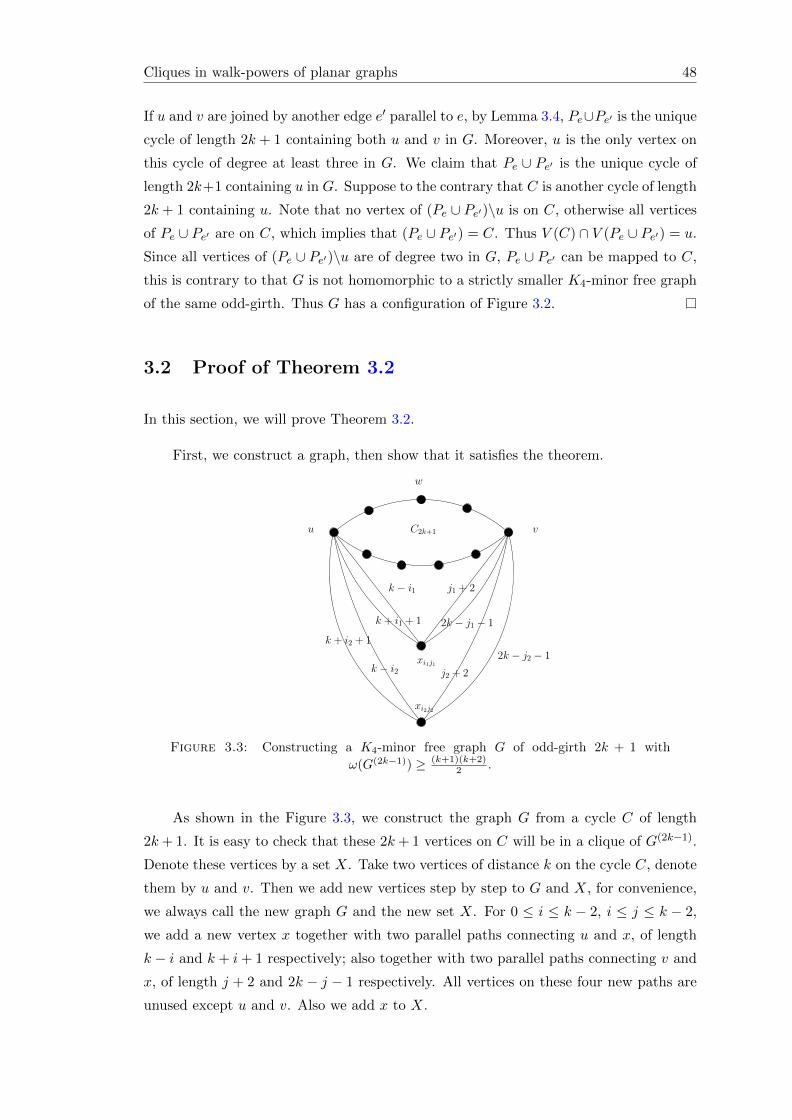
Cliques in walk-powers of planar graphs 48
If u and v are joined by another edge e′ parallel to e, by Lemma 3.4, Pe∪Pe′ is the unique
cycle of length 2k + 1 containing both u and v in G. Moreover, u is the only vertex on
this cycle of degree at least three in G. We claim that Pe ∪ Pe′ is the unique cycle of
length 2k+1 containing u in G. Suppose to the contrary that C is another cycle of length
2k + 1 containing u. Note that no vertex of (Pe ∪ Pe′)\u is on C, otherwise all vertices
of Pe ∪ Pe′ are on C, which implies that (Pe ∪ Pe′) = C. Thus V (C) ∩ V (Pe ∪ Pe′) = u.
Since all vertices of (Pe ∪ Pe′)\u are of degree two in G, Pe ∪ Pe′ can be mapped to C,
this is contrary to that G is not homomorphic to a strictly smaller K4-minor free graph
of the same odd-girth. Thus G has a configuration of Figure 3.2.
3.2 Proof of Theorem 3.2
In this section, we will prove Theorem 3.2.
First, we construct a graph, then show that it satisfies the theorem.
w
u v
k − i1
k + i1 + 1
k + i2 + 1
j1 + 2
2k − j2 − 1k − i2 j2 + 2
2k − j1 − 1
C2k+1
xi1j1
xi2j2
Figure 3.3: Constructing a K4-minor free graph G of odd-girth 2k + 1 with
ω(G(2k−1)) ≥ (k+1)(k+2)2 .
As shown in the Figure 3.3, we construct the graph G from a cycle C of length
2k+ 1. It is easy to check that these 2k+ 1 vertices on C will be in a clique of G(2k−1).
Denote these vertices by a set X. Take two vertices of distance k on the cycle C, denote
them by u and v. Then we add new vertices step by step to G and X, for convenience,
we always call the new graph G and the new set X. For 0 ≤ i ≤ k − 2, i ≤ j ≤ k − 2,
we add a new vertex x together with two parallel paths connecting u and x, of length
k − i and k + i+ 1 respectively; also together with two parallel paths connecting v and
x, of length j + 2 and 2k − j − 1 respectively. All vertices on these four new paths are
unused except u and v. Also we add x to X.
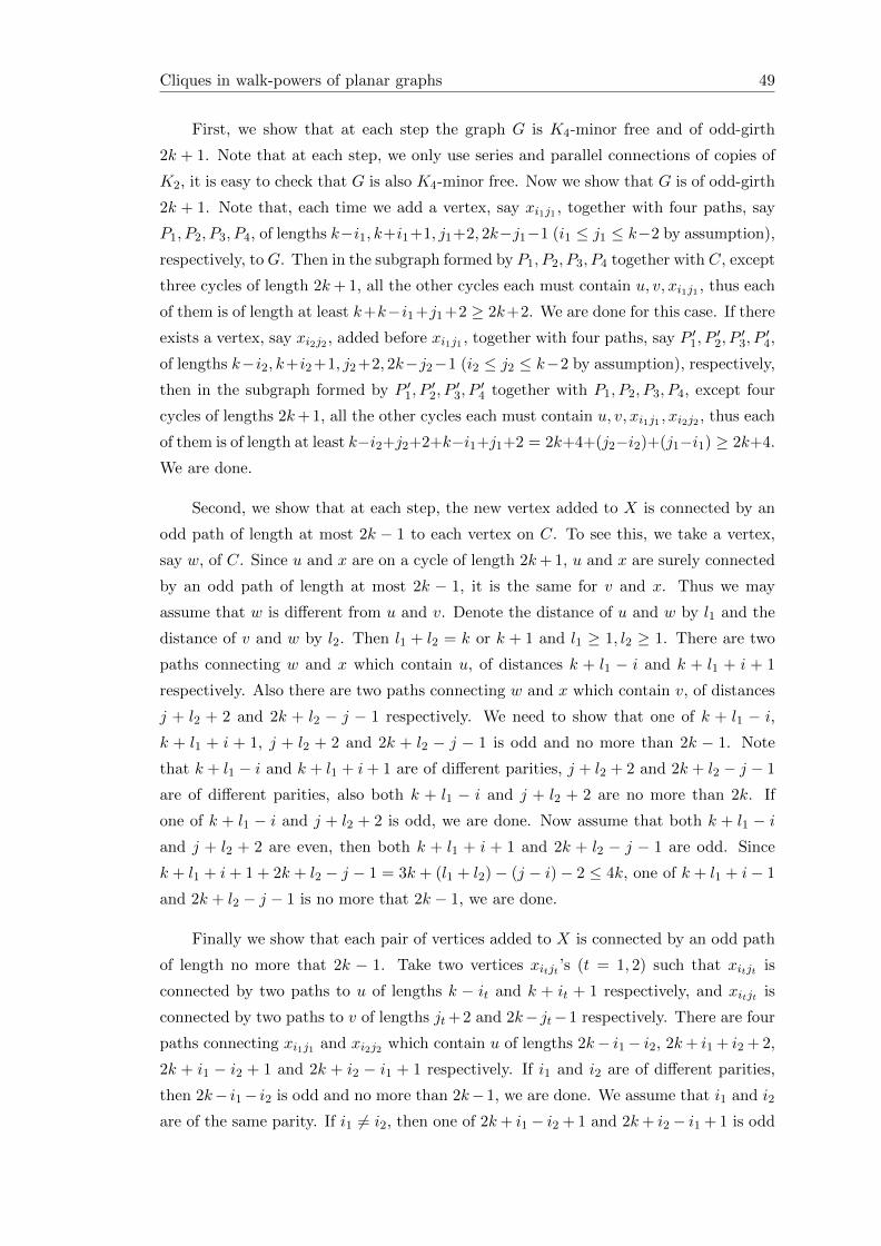
Cliques in walk-powers of planar graphs 49
First, we show that at each step the graph G is K4-minor free and of odd-girth
2k + 1. Note that at each step, we only use series and parallel connections of copies of
K2, it is easy to check that G is also K4-minor free. Now we show that G is of odd-girth
2k + 1. Note that, each time we add a vertex, say xi1j1 , together with four paths, say
P1, P2, P3, P4, of lengths k−i1, k+i1+1, j1+2, 2k−j1−1 (i1 ≤ j1 ≤ k−2 by assumption),
respectively, toG. Then in the subgraph formed by P1, P2, P3, P4 together with C, except
three cycles of length 2k+ 1, all the other cycles each must contain u, v, xi1j1 , thus each
of them is of length at least k+k−i1 +j1 +2 ≥ 2k+2. We are done for this case. If there
exists a vertex, say xi2j2 , added before xi1j1 , together with four paths, say P ′1, P′2, P
′3, P
′4,
of lengths k−i2, k+i2 +1, j2 +2, 2k−j2−1 (i2 ≤ j2 ≤ k−2 by assumption), respectively,
then in the subgraph formed by P ′1, P′2, P
′3, P
′4 together with P1, P2, P3, P4, except four
cycles of lengths 2k+ 1, all the other cycles each must contain u, v, xi1j1 , xi2j2 , thus each
of them is of length at least k−i2+j2+2+k−i1+j1+2 = 2k+4+(j2−i2)+(j1−i1) ≥ 2k+4.
We are done.
Second, we show that at each step, the new vertex added to X is connected by an
odd path of length at most 2k − 1 to each vertex on C. To see this, we take a vertex,
say w, of C. Since u and x are on a cycle of length 2k+ 1, u and x are surely connected
by an odd path of length at most 2k − 1, it is the same for v and x. Thus we may
assume that w is different from u and v. Denote the distance of u and w by l1 and the
distance of v and w by l2. Then l1 + l2 = k or k + 1 and l1 ≥ 1, l2 ≥ 1. There are two
paths connecting w and x which contain u, of distances k + l1 − i and k + l1 + i + 1
respectively. Also there are two paths connecting w and x which contain v, of distances
j + l2 + 2 and 2k + l2 − j − 1 respectively. We need to show that one of k + l1 − i,k + l1 + i + 1, j + l2 + 2 and 2k + l2 − j − 1 is odd and no more than 2k − 1. Note
that k + l1 − i and k + l1 + i+ 1 are of different parities, j + l2 + 2 and 2k + l2 − j − 1
are of different parities, also both k + l1 − i and j + l2 + 2 are no more than 2k. If
one of k + l1 − i and j + l2 + 2 is odd, we are done. Now assume that both k + l1 − iand j + l2 + 2 are even, then both k + l1 + i + 1 and 2k + l2 − j − 1 are odd. Since
k + l1 + i+ 1 + 2k + l2 − j − 1 = 3k + (l1 + l2)− (j − i)− 2 ≤ 4k, one of k + l1 + i− 1
and 2k + l2 − j − 1 is no more that 2k − 1, we are done.
Finally we show that each pair of vertices added to X is connected by an odd path
of length no more that 2k − 1. Take two vertices xitjt ’s (t = 1, 2) such that xitjt is
connected by two paths to u of lengths k − it and k + it + 1 respectively, and xitjt is
connected by two paths to v of lengths jt+2 and 2k− jt−1 respectively. There are four
paths connecting xi1j1 and xi2j2 which contain u of lengths 2k− i1− i2, 2k+ i1 + i2 + 2,
2k + i1 − i2 + 1 and 2k + i2 − i1 + 1 respectively. If i1 and i2 are of different parities,
then 2k− i1− i2 is odd and no more than 2k−1, we are done. We assume that i1 and i2
are of the same parity. If i1 6= i2, then one of 2k+ i1− i2 + 1 and 2k+ i2− i1 + 1 is odd

Cliques in walk-powers of planar graphs 50
and no more than 2k − 1, we are done. Thus we assume that i1 = i2. Since xi1j1 and
xi2j2 are distinct, j1 6= j2. Then there are four paths connecting xi1j1 and xi2j2 which
contain v of lengths j1 + j2 + 4, 4k − j1 − j2 − 2, 2k + j1 − j2 + 1 and 2k + j2 − j1 + 1
respectively. If j1 and j2 are of different parities, then j1 + j2 + 4 is odd and no more
that 2k− 1, we are done. If j1 and j2 are of the same parity, then one of 2k+ j1− j2 + 1
and 2k + j2 − j1 + 1 is odd and no more than 2k − 1, we are done.
Now we calculate the size of X. At beginning, there are 2k+ 1 vertices in X. Each
pair (i, j) gives a new vertex, where 0 ≤ i ≤ k − 2 and i ≤ j ≤ k − 2. Thus there are
(k−2+1)+(k−2)+. . .+1 new vertices. Totally, we get |X| = 1+2+. . .+k−1+2k+1 =(k+1)(k+2)
2 .
The proof of Theorem 3.2 is completed.
3.3 Preliminaries for the proof of Theorem 3.3
In this section, we give some Lemmas for the proof of Theorem 3.3.
Lemma 3.7. Let G be a graph and C be a cycle of length at least 3 in G. If there exist
3 walks, say W1,W2,W3, starting from x in G\C such that the first vertex where Wi
meets C is xi (i = 1, 2, 3), where x1, x2 and x3 are mutually distinct, then G has K4 as
a minor.
Proof. Denote by T the component containing x in G\C. It is easy to check that xi
(i = 1, 2, 3) is adjacent to a vertex in H. Contract T to be a new vertex x′, then x′ is
adjacent to all of x1, x2, x3. Contract some edges of C such that x1, x2 and x3 are
mutually adjacent, then we get a K4 as a minor.
Lemma 3.8. Let G be a K4-minor free graph of odd-girth 5. Let X be a set of vertices
of a clique in G(3). Then for any vertex w, |N1(w) ∩X| ≤ 2.
Proof. Suppose to the contrary that there exists a vertex w adjacent to 3 vertices
x1, x2, x3 in X. Since x1 and x2 are in X, there exists a 3-walk W connecting them
in G. Then W together with x2wx1 walk forms a closed walk of length 5. Thus it
should contain an odd-cycle of length at most 5. Since G is triangle free, this closed
walk should be a 5-cycle, denote it by Cx1x2 . We claim that x3 is not on Cx1x2 . To see
this, note that two neighbors of w in Cx1x2 are x1 and x2. If x3 is also one of vertices of
Cx1x2 , then since x3 is adjacent to w, we will have a smaller odd-cycle.
Similarly, since x3 and x1 are in X, there exists a 3-walk W1 connecting them in
G. Then W1 together with x1wx3 walk forms a 5-cycle, and x2 is not on it. Denote
Cliques in walk-powers of planar graphs 51
by w1 the vertex where W1 meets W . Note that w1 6= x2. Since W is of length 3, the
lengths of w1x1 walk and w1x2 walk in W have different parities. Thus x3w1 walk in
W1 together with w1x2 walk in W is of even length, and W1 together with x1wx2 walk
is of length 5. We need another 3-walk W2 connecting x3 and x2 in G. Similarly, W2
together with x2wx3 walk forms a 5-cycle, and x1 is not on it. Denote by w2 the vertex
where W2 meets W . Note that w2 6= x1.
We claim that w1 6= w2. To the contrary, let w1 = w2. Note that x2 6= w1, x1 6= w2.
Then W1 together with x1wx2 walk and W2 is a closed walk of length 8, which contains
Cx1x2 of length 5. Thus x3w1 walk in W1 together with x3w2 walk in W2 is a closed
walk of length 3, a contradiction.
Since x3 is adjacent to w, W1 and W2 meet Cx1x2 at another two different vertices
w1 and w2, by Lemma 3.7, we can get a K4 as a minor. A contradiction.
In this Lemma we show that, at most 2 vertices in N(w) of any w can form a clique
in G(3), in the following, we show that at most 3 vertices in N2(w) of any w can form a
clique in G(3).
Lemma 3.9. Let G be a K4-minor free graph of odd-girth 5. Let X be a set of vertices
of a clique in G(3). Then for any vertex w, |N2(w) ∩X| ≤ 3.
Proof. Suppose to the contrary that there exist a vertex w and four vertices x1, x2, x3, x4
such that x1, x2, x3, x4 ⊆ N2(w) ∩X. Since x1 and x2 are in X, there exists a 3-walk
W connecting them in G. Respect to the existence of common neighbors of x1 and x2
in N1(w), we continue our proof in two cases.
Case 1. N1(x1) ∩ N1(x2) ∩ N1(w) 6= ∅. Denote one of the common neighbors of
w and xi’s (i = 1, 2) by w1. Since x1, x2 ⊆ X, there exists a 3-walk connecting
x1 and x2, denote it by x1y1y2x2. Note that G is triangle free, it is to check that
y1, y2 ∩ x1, x2, w1, w = ∅.
Subcase 1. |x3, x4∩y1, y2| = 2. Note that G is triangle free, w1 is not adjacent
to y1 or y2, moreover, y1 and y2 has no common neighbors. Since w1x1y1y2x2w1 forms a
cycle of length 5, denoted C, and there exist 3 walks starting from w in G\C such that
the first vertices they meet C are w1, y1 and y2 respectively. By Lemma 3.7, G has a
K4 as a minor, a contradiction.
Subcase 2. |x3, x4 ∩ y1, y2| = 1. Assume w.l.o.g. that x3 = y1. Since G is
triangle free, y1 is not adjacent to w1. Note that y1 = x3 ∈ N2(w), y1 and w must
have a common neighbor. We claim that this common neighbor could be not one of
w1, x1, x2, otherwise there will be a triangle, a contradiction.

Cliques in walk-powers of planar graphs 52
First, we assume that y2 is one of the common neighbors of w and y1. By Lemma
3.8, x4 is not adjacent to w1. Note that x4 ∈ N2(w).
If x4 is adjacent to y2, the x2, x3, x4 ⊆ X ∩N(y2), a contradiction by Lemma 3.8.
If x4 is not adjacent to y2, denote by y3 the common neighbor of w and x4, then
y3 /∈ w1, x1, x2, y1, y2. There are 3-walks connecting x4 and x1, x2, y1 respectively.
Considering the distances between w and xi’s, none of these 3-walks contains w. Simi-
larly to the proof in Lemma 3.8, the number of the first vertices where these 3-walks meet
the cycle w1x1y1y2x2w1 must be at least 2. In this case, there are walks starting from
x4 which meet one of the cycles ww1x2y2 and ww1x1y1y2 at three distinct vertices(first
meet vertices). Then by Lemma 3.7 we get a contradiction.
Second, we assume that y2 is not the common neighbor of w and y1. This case is
very similar to case that the common neighbor of y1 and w is y2, we can use Lemma 3.7
to get a contradiction.
Subcase 3. |x3, x4 ∩ y1, y2| = 0. By Lemma 3.8, both x3 and x4 are not
adjacent to w1. Note that w1x1y1y2x2w1 is a cycle of length 5, denote it by C, to get
two 3-walks connecting xi (i = 3, 4) and x1 or x2, there are two ways: one is connecting
x3 to w1 by a 2-walk, the other one is connecting x3 by two walks which meet C at two
different vertices. It is the same for x4. We only give one case here: x3 is connected to
w1 by a 2-walk, and x4 is connected by two walks to C which meet C at two different
vertices except w1. In this case, since x3 and x4 is connected by 3-walk and x3 is
connected to w1 by a 2-walk, it is easy to check that there is a walk connecting x4 and
w1 such that w1 is the first vertex where the walk meets C. Thus, by Lemma 3.7 we get
a contradiction. The other cases are similar.
Case 2. N1(x1)∩N1(x2)∩N1(w) = ∅. Moreover, we can assume N1(xi)∩N1(xj)∩N1(w) = ∅ (i 6= j, i, j ⊆ 1, 2, 3, 4), otherwise it is the same as Case 1. Denote one
of the common neighbors of w and xi by yi (i = 1, 2, 3, 4). Note that yi’s are distinct.
First, we claim that no pair of xi and xj are adjacent. To see this, suppose to the
contrary we assume that x1 and x2 are adjacent. Then wy1x1x2y2w is a cycle of length
5, denoted it C. Assume that W1 and W2 are two 3-walks connecting x3 to x1 and
x2, then W1 and W2 do not contain w. Moreover, the first vertices W1 and W2 meet
C must be the same, otherwise by Lemma 3.7 we get a contradiction. Thus the only
way is that one of W1,W2 is of length 2, the other is of length 3, W1 and W2 meet
at x1 or x2, say x2. Note that x3 could not be adjacent to x1 or x2. In this case there
must exist a cycle containing w, x1, x2, x3, denote it by C ′. Now consider the 3-walks,
say W3,W4,W5, connecting x4 to xi’s (i = 1, 2, 3). Since w and xi (i = 1, 2, 3, 4) are of
distance 2, W3,W4,W5 do not contain w. Furthermore, since x2 is of different distance

Cliques in walk-powers of planar graphs 53
to x1 and x3 on C ′, W3,W4,W5 must meet C ′ at at least 2 vertices, then together with
x4y4w, there are 3 walks starting from x4 which meet C ′ at three distinct vertices, we
get a contradiction by Lemma 3.7.
Second, we claim that no pair of xi and xj are connected by a 3-walk without using
vertices in y1, y2, y3, y4. To see this, suppose to the contrary we assume that x1 and
x2 are connected by a 3-walk x1y5y6x2. Thus wy1x1y5y6x2y2w form a cycle of length 7,
denoted by C. Once again, let W1 and W2 be two 3-walks connecting x3 to x1 and x2,
respectively. Considering the distance between x1 and x2, W1 and W2 must meet C at
two distinct vertices. Including the walk x3y3w, there are three walks starting from x4
which meet C at three distinct vertices, by Lemma 3.7 a contradiction.
Furthermore, we claim that no pair of xi and xj are connected by a 3-walk using
two vertices in y1, y2, y3, y4, otherwise a triangle arises.
Thus each pair of xi and xj are connected by a 3-walk using exactly one vertex in
y1, y2, y3, y4 and one vertex not in w, xi, yi (i = 1, 2, 3, 4). Since there are C24 = 6
pairs of xi and xj , and there are only 4 yi’s, on these six 3-walks, there are two cases:
one of yi’s is used 3 times and the others each is used once; two of yi’s are used twice
and the others each is used once. We give the proof of the first case here, the second
case is similar. Assume w.l.o.g that y1 is used 3 times in the 3-walks connecting x1 to
x2, x3 or x4. On these three 3-walks, y1 can be adjacent to 1, 2 or 3 new vertices. We
give the proof for the case y1 adjacent to one new vertex, say y∗1, the other cases are
similar. These three 3-walks are x1y1y∗1xi (i = 2, 3, 4). Moreover, assume x2 and x3
are connected by a 3-walk x2y2y∗2x3. Note that y∗2 6= y∗1, otherwise a triangle arises.
Now wy2y∗2x3y3w form a cycle of length 5, denote it by C. Then there are three walks
starting from x3 which meet C at three distinct vertices y2, x3 and w, by Lemma 3.7 we
get a contradiction.
This completes the proof.
Lemma 3.10. Let G be a K4-minor free graph of odd-girth 5. Let u and v be two
vertices of G connected by a thread of length at least 2. For any two vertices x, y in
V (G)\u, v, if d(x, u) = d(y, u) = 2 and d(x, v) = d(y, v) = 1, then x and y are not
adjacent in G(3).
Proof. Suppose to the contrary that x and y are adjacent in G(3), that means there
exists a 3-walk W connecting them in G, considering the distances between x, y and
u, v, x, y are not on this thread. Since d(x, u) = d(y, u) = 2, u and x have a common
neighbor, denote it by w1. And u and y also have a common neighbor, denote it by w2.
Cliques in walk-powers of planar graphs 54
Note that the vxw1u walk together with uv-thread forms a cycle, denoted C, of length
at least 5.
We claim that u is not on W , otherwise, since W is of length 3, u is adjacent to
either x or y, which is contrary to d(x, u) = d(y, u) = 2. Note that W together with
xvy walk forms a closed walk of length 5, thus it should contain an odd-cycle of length
at most 5. Since G is triangle free, this closed walk should be a 5-cycle, that means v is
not on W .
If w1 = w2, similarly to v, we can prove that w1 is not on W . Now there exist 3
walks starting from y which meet C at 3 different vertices w1, v and x. By Lemma 3.7,
G has a K4 as a minor, a contradiction.
If w1 6= w2, then one of w1,w2 is not on W , otherwise w1 and w2 are adjacent
and a triangle uw1w2 arises, a contradiction. If one of w1, w2, assume w.l.o.g. w1, is
on W , then there exist 3 walks starting from y which meet C at 3 different vertices u, v
and x. By Lemma 3.7, G has a K4 as a minor, a contradiction. If neither w1 nor w2 is
on W , then there exist 3 walks starting from y which meet C at 3 different vertices u, v
and x. By Lemma 3.7, G has a K4 as a minor, a contradiction.
This completes the proof.
3.4 Proof of Theorem 3.3
Now we prove the Theorem 3.3.
Given two graphs G and H, if G → H, then any clique in G will be mapped to
a clique of same size in H. Thus ω(G) ≤ ω(H). If ϕ is a homomorphism of G to H,
then by Lemma 2.19 ϕ is also a homomorphism of G(k) to H(k). Define a class G of
graphs such that every member of G is K4-minor free graph of odd-girth 5 and is not
homomorphic to a strictly smaller K4-minor free graph of the same odd-girth. Note
that every K4-minor free graph of odd-girth 5 is homomorphic to a member of G. To
prove the Theorem 3.3, we only need to prove that every graph G ∈ G, ω(G(3)) ≤ 6.
Suppose to the contrary that there exists counterexamples in G, take one of minimum
order, denote it by G. Note that ω(G(3)) ≥ 7, since ω(C(3)5 ) = 5, G 9 C5. Thus by
Corollary 3.6 G has a configuration either in Figure 3.4 or in Figure 3.5. Let X be a
set of vertices of a maximum clique in G(3), then |X| ≥ 7. We will get contradictions
according to the two configurations of G.

Cliques in walk-powers of planar graphs 55
G′
y3 y6
y7
y5
y4y2
x z
y
y1
Figure 3.4: Con-figuration 3
u
v2
v1
v3
v4
C5
Figure 3.5: Con-figuration 4
3.4.1 G has a configuration in Figure 3.5
Firstly, we claim that v1, v2, v3, v4 ∩X 6= ∅. To see this, assume that v1, v2, v3, v4 ∩X = ∅, then X ⊆ V (G)\v1, v2, v3, v4. For any two vertices in X connected by a 3-walk
W , if one of v1, v2, v3, v4 is on W , then all of them are on W , contrary to that W is
a 3-walk. Thus none of v1, v2, v3, v4 is on a 3-walk connecting a pair of vertices in X.
Deleting the vertices in v1, v2, v3, v4, we get a smaller counterexample, a contradiction.
Secondly, we claim that v1, v4∩X 6= ∅ and v2, v3∩X = ∅. To see this, suppose
that v2, v3 ∩X 6= ∅. Assume w.l.o.g. that v2 ∈ X. If v1 ∈ X, since |X| ≥ 7, there are
at least two vertices w1, w2 in X ∩ V (G\C5), Note that d(v2, u) = 2 and there exists a
3-walk connecting v2 and each of w1, w2, we get that w1 and w2 must be adjacent to u.
Now three neighbors of u are in X, by Lemma 3.8, we get a contradiction. If v1 /∈ X,
since |X| ≥ 7, there are at least 3 vertices in X ∩ V (G\C5) which must be adjacent to
u, a contradiction by Lemma 3.8. Therefor, v2, v3 ∩X = ∅ and v1, v4 ∩X 6= ∅.
Since v1, v4 ∩X 6= ∅, assume w.l.o.g that v1 ∈ X. Note that |X| ≥ 7, there are
at least 4 vertices of X in X ∩ V (G\C5), which are in N2(u). By Lemma 3.9, we get a
contradiction.
3.4.2 G has a configuration in Figure 3.4
We first claim that at most one of y1, y5 is in X. To see this, note that any walk W
connecting y1 and y5, W contains either y or both z and x. If W contains y, then it is
of even length or of length at least 5. If W contains both z and x, then it is of length at
least 6. Thus there is no walk of length 3 connecting y1 and y5, at most one of y1, y5could be in X. Similarly we can prove that at most one of y2, y6, one of y1, y4, one
of y6, y7, one of y3, y4, y7 could be in X. Note that at most 3 of y1, y2, . . . , y7could be in X. Considering y is in X or not, there are two cases.

Cliques in walk-powers of planar graphs 56
Case 1. Vertex y ∈ X. Note that 3 of y1, y2, . . . , y7 together with x, y, z, we now
have at most 6 vertices in X. Since |X| ≥ 7, there exists at least one vertex w1 in G′
such that w1 ∈ X, w1 /∈ z, x. Thus there exists a 3-walk connecting w1 to y. Since
d(y, x) = d(y, z) = 2, w1 must be adjacent to x or z. Assume w.l.o.g. that w1 is adjacent
to x. We show that y2 /∈ X. To see this, if there exists a 3-walk W connecting y2 to w1,
the y2xw1 walk together W forms a 5-walk. Note that y2 is on the unique 5-cycle, this
5-walk must contain a cycle of length 3, a contradiction. Similarly, we can show that
y3 /∈ X.
If y1 ∈ X, then y4 /∈ X, y5 /∈ X. Since at most one of y6, y7 could be in X,
together with x, y, z, w1, y1, now we have at most 6 vertices in X. Since |X| ≥ 7, there
exists another vertex w2 in G′ such that w2 ∈ X, w2 /∈ z, x. Since d(y1, x) = 2 and
d(y1, z) = 3, to connect y1 with w2 by a 3-walk, w2 must be adjacent to x. Moreover,
for any vertex w in G′ such that w ∈ X, w /∈ z, x, w must be adjacent to x. By
Lemma 3.8, at most two neighbors of x could be in X. Thus one of y6, y7 must be in
X. Since y7 is adjacent to x, y7 /∈ X. Therefor, y6 ∈ X. Since d(y6, x) = 3, d(y6, z) = 1,
y6 and wi(i = 1, 2) are connected by a 3-walk, we can get that d(w1, z) = d(w2, z) = 2.
Together with d(w1, x) = d(w2, x) = 1 and by Lemma 3.10, w1 and w2 could not be
adjacent in G(3), a contradiction.
If y1 /∈ X. Now y5 could be in X. If y5 ∈ X, since d(y5, z) = 2 and (y5, x) = 3, for
any vertex w in G′ such that w ∈ X, w /∈ z, x, w must be adjacent to z. By Lemma
3.8, at most two neighbors of z could be in X, together with z, x, y, y5, we have at most
6 vertices in X, a contradiction. If y5 /∈ X. By Lemma 3.8, at most 3 of z ∪N(z) can
be in X, together with y, z, w1, we now have at most 6 vertices in X. Since |X| ≥ 7,
there exists another vertex w2 in G′ such that w2 ∈ X, w2 /∈ z, x, moreover w2 /∈ N(z)
and w2 is connected to y by a 3-walk, thus w2 is adjacent to x. In this case, if one of
y4, y6, y7 is in X, then d(w1, z) = d(w2, z) = 2. together with d(w1, x) = d(w2, x) = 1,
and by Lemma 3.10, w1 and w2 could not be adjacent in G(3), a contradiction. If none of
y4, y6, y7 is in X, now we have 5 vertices y, z, x, w1, w2 in X, Since |X| ≥ 7, there exists
another two vertex w3, w4 in G′ such that w3 ∈ X, w4 ∈ X, w3 /∈ z, x, w4 /∈ z, x.Note that w3 and w4 are adjacent to z or x, by Lemma 3.8, both of them are adjacent
to z. In this case, w1, w2, w3, w4 ⊆ N2(y7), by Lemma 3.9 we get a contradiction.
Case2. Vertex y /∈ X. It is easy to check that y can be connected by a 3-walk
to each of x, z, y1, y2, . . . , y7. If none of y1, y2, . . . , y6 is in X, note that no pair of
vertices in X are connected by a 3-walk containing a vertex in y, y1, y2, . . . , y6, then
deleting vertices in y, y1, y2, . . . , y6, we get a smaller counterexample, a contradiction.
Thus at least one of y1, y2, . . . , y6 is in X. Note that at most 3 of y1, y2, . . . , y7 could

Cliques in walk-powers of planar graphs 57
be in X. Together with x, z, we now have at most 5 vertices in X, thus at least two
vertices in X which are in G′\z, x.
If one of y1, y5 is in X, then all vertices in X which are in G′\z, x are adjacent
to x or z, thus y is connected to each of them by a 3-walk, we get a bigger clique with
vertex set X ∪ y, a contradiction.
If y1 /∈ X, y5 /∈ X. We claim that at least one of y4, y6 is in X, otherwise, note
that now X ⊆ V (G′)∪y2, y3, none of y4, y5, y6 is necessarily on a 3-walk connecting
a pair of vertices in X, deleting them we get a smaller counterexample, a contradiction.
It is same for y2, y3. Since at most one of y2, y6 could be in X, at most one of y3, y4could be in X, assume w.l.o.g. that y3 and y6 are in X. Now none of y1, y2 is on a 3-
walk connecting a pair of vertices in X, deleting them we get a smaller counterexample,
a contradiction.
The proof of Theorem 3.3 is completed.
3.5 Other cases of Conjecture 3.1
Even though we have not proved the other cases of Conjecture 3.1, we get some partial
results.
Claim 3.11. Given a graph G of odd-girth at least 2k+1 and a u, v-thread P of length lp
in G, denote the set of internal vertices of P by S. For any two vertices x, y in V (G\P ),
assume that in the graph induced by V (G) \ S, W is a walk connecting x and y of odd
length l, P1, P2, P3, P4, are shortest paths connecting x and v, y and v, x and u, y and
u respectively, with Pi being of length of li, 1 ≤ i ≤ 4, satisfying: V (P1) ∩ V (P2) = v,
V (P3) ∩ V (P4) = u, l1 ≡ l2 (mod 2), l3 ≡ l4 (mod 2), and l + li 2k + 1 for 1 ≤ i ≤ 4.
Then G has K4 as a minor.
Proof. First, we claim that none of the vertices of P is on W . Too see this, suppose that
V (P ) ∩ V (W ) 6= ∅, thus there are two cases.
Case 1. |V (W ) ∩ V (P )| = 1. Assume w.l.o.g. that V (W ) ∩ V (P ) = v. Then W
together with P1 and P2 forms a closed walk W ′. Since l1 ≡ l2 (mod 2), l is odd, W ′ is of
odd length. Thus W ′ contains an odd-cycle C which is formed by part of P1, or part of
P2, together with W . Since l+ li 2k + 1 for 1 ≤ i ≤ 4, |C| ≤ l+ maxl1, l2 ≤ 2k− 1,
which is contrary to that the odd-girth of G is at least 2k + 1.
Case 2. V (W ) ∩ V (P ) = V (P ). Then W must be formed by a x, v-walk, say W1,
together with v, u-thread and a u, y-walk, say W2. Then W together with P4 and P3

Cliques in walk-powers of planar graphs 58
forms a closed walk W ′ with length l + l3 + l4. If W1 together with v, u-thread and P3
forms a closed walk of odd length, then it contains an odd-cycle of length smaller than
l + l3 2k + 1, a contradiction. Thus W ′ contains an odd-cycle formed by W and part
of P4, which is of length smaller that l + l4 2k + 1, a contradiction.
Now, we prove that G contains a K4 as a minor. Note that P1 together with P and
P3 forms a cycle of length at least 3, denote it by C ′. Let W start from y, denote the
first vertex where W meets C ′ by w. Since V (P ) ∩ V (W ) = ∅, w, u, v are distinct. By
Lemma 3.7, G has a K4 as a minor.
Next we generalize the Lemma 3.8 to general odd-girth.
Claim 3.12. Let G be a K4-minor free graph of odd-girth 2k+ 1, k ≥ 1. Let X be a set
of vertices of a clique in G(2k−1). Then for any vertex w, |N(w) ∩X| ≤ 2.
Proof. The proof of this Lemma is very similar to Lemma 3.8. Suppose to the contrary
that there exists a vertex w adjacent to 3 vertices x1, x2, x3 in X. Since x1 and x2 are
in X, there exists a (2k − 1)-walk W connecting them in G. Then W together with
x2wx1 walk forms a closed walk of length 2k + 1. Thus it should contain an odd-cycle
of length at most 2k + 1. Since G is of odd-girth 2k + 1, this closed walk should be a
(2k + 1)-cycle, denote it by Cx1x2 . We claim that x3 is not on Cx1x2 . To see this, note
that two neighbors of w in Cx1x2 are x1 and x2. If x3 is also one of vertices of Cx1x2 ,
since x3 is adjacent to w, we will have a smaller odd-cycle, a contradiction.
Similarly, since x3 and x1 are in X, there exists a (2k − 1)-walk W1 connecting
them in G. Then W1 together with x1wx3 walk forms a (2k + 1)-cycle, denoted Cx1x3 ,
and x2 is not on Cx1x3 . Denote by w1 the first vertex where W1 meets Cx1x2 . Note
that w1 6= x2, w. Since W is of length 2k − 1, the w1x1-walk and w1x2-walk in W have
different parities. Without of losing generality, we assume that w1x1-walk in W is of
even length l1 and w1x2-walk in W is of odd length l2 such that l1 + l2 = 2k − 1. In
the one hand, since x3w1-walk in W ′ together with w1x1 walk in W , which actually
forms W1, is of an odd length 2k − 1, x3w1-walk in W1 together with w1x2 walk in W
forms a even walk. On the other hand, W1 together with x1wx2-walk forms a walk of
length 2k + 1 which is greater than 2k − 1. We need another walk, say W2, of length
(2k − 1), connecting x3 and x2 in G. Similarly, W2 together with x2wx3-walk forms a
(2k + 1)-cycle, denoted Cx2x3 , and x1 is not on Cx2x3 . Denote by w2 the vertex where
W2 meets Cx2,x3 . Note that w2 6= x1, w.
We claim that w1 6= w2. To the contrary, let w1 = w2. Note that x2 6= w1 = w2 6=x1. Then W1 together with x1wx2 walk and W2 forms a closed walk of length 2k, which

Cliques in walk-powers of planar graphs 59
contains Cx1x2 of length 2k + 1, thus there must exist an odd-cycle of at most 2k− 1, a
contradiction.
This completes the proof.
3.6 Concluding remarks and further work
In this chapter, we consider the clique number of the (2k− 1)-walk-powers of K4-minor
free graphs of odd girth 2k + 1. We conjectured that the upper bound is (k+1)(k+2)2 .
First, we constructed a graph such that this upper bound is achieved. Our result
together with the result from [6] implies that order O(k2) is optimal for the graphs of
odd-girth that bounding all K4-minor free graphs of odd-girth 2k + 1.
Then, we show that for k = 2, our conjecture holds. We hope to prove the general
cases of the conjecture.

Chapter 4
Homomorphism and planar
graphs
In this chapter, we will discuss some results related to Problem 1.14 and Conjecture
1.20. To make it easier to read, we state again the problems here.
Problem 4.1. [81] Given integers l ≥ k ≥ 1, what are the minimal subgraphs of PC(2k)
to which every planar graph of odd-girth 2l + 1 admits a homomorphism?
In [81], Naserasr conjectured that K(2k + 1, k), as a subgraph of PC(2k), is an
answer for the case r = k + 1. The first case of Problem 4.1 which is not being studied
is k = 3 and r = 5. For this case, we conjecture that the Coxeter graph, which is a
subgraph of K(7, 3), bounds the planar graph of odd-girth at least 11. We state again
the Conjecture 1.20 here.
Conjecture 4.2. [46] Every planar graph of odd-girth at least 11 admits a homomor-
phism to the Coxeter graph.
Supporting this conjecture, we prove Theorem 1.21. We state again this theorem
here.
Theorem 4.3. [46] Every planar graph of odd-girth at least 17 admits a homomorphism
to the Coxeter graph.
We will prove this theorem by contradiction and discharging technique. In section
4.1 we will present a list properties of Kneser graphs and Coxeter graph. In section 4.2,
we present the folding lemma which is used to characterize the faces a plane graph and
Euler formula which is used to give an initial charge. In section 4.3, we assume there
exists a counterexample and give a list of ten reducible configurations. In section 4.4,
we will use discharging technique to obtain a contradiction.
60

Homomorphism and planar graphs 61
4.1 Kneser graphs and Coxeter graph
Recall that the Kneser graph K(n, k), n ≥ 2k, is defined to be the graph whose vertices
corresponding to the k-element subsets of a set of n elements, and where two vertices are
adjacent if and only if the two corresponding sets are disjoint. Kneser graphs are named
after Martin Kneser, who first investigated them in 1955. Kneser graph K(2k−1, k−1)
is the well-known odd graph, usually denoted O(k).
It is well-known that Kneser Graph K(n, k) is both vertex-transitive and edge-
transitive. For the Kneser graph K(n, k), if n = 2k, then K(n, k) is a matching; if
k = 1, then K(n, k) is isomorphic to Kn. K(5, 2) is isomorphic to the well-known
Petersen graph and O(3). K(7, 3) is isomorphic to O(4).
It is shown that K(2k+ 1, k) is isomorphic to an induced subgraph of PC(2k) (see
[81]). Here we show this fact by giving an isomorphic mapping from K(2k + 1, k) to an
induced subgraph of PC(2k).
Proposition 4.4. K(2k + 1, k) is isomorphic to an induced subgraph of PC(2k).
Proof. In the binary representation of PC(2k), vertices are the elements of Z2k2 , PC(2k) =
(Z2k2 , e1, e2, . . . , e2k, J) where ei’s are the standard basis of Z2k
2 and J is the all 1 vector
of length 2k. Denote the set of all vertices with k 1’s by U and the set of all vertices
with k − 1 1’s by V . Note that the subgraph induced by U ∪ V in PC(2k) is of order(2kk
)+(
2kk−1
)=(
2k+1k
). Moreover, in this induced subgraph, x− y = J only if x, y ∈ U ,
x− y = ei only if one of x, y is in U and the other is in V .
For any vertex u in U , we extend u to an element, denoted u′, of Z2k+12 by the
following operations: first, take a complement of u, which is u + J ; second, add a
(2k + 1)-th coordination with 0 to u + J . For any vertex v in V , we extend v to an
element, denoted v′, of Z2k+12 by adding a (2k+ 1)-th coordination with 1 to v, denoted
u+ e2k+1. Note that this is an one-to-one extension. Denote the set of u′ by U ′, the set
of v′ by V ′.
Now we present the vertices of K(2k+1, k) as the elements of Z2k+12 . Denote the set
of 2k + 1 elements by 1, 2, . . . , 2k + 1. Given a k-set, i1, i2, . . . , ik, take the element
of Z2k+12 with ij ’th coordination 1, 1 ≤ j ≤ i, to correspond to it. It is easy to check
that, the vertices of K(2k+ 1, k) can be presented as vertices in U ′ ∪ V ′. Note that two
vertices, say x and y, of K(2k + 1, k) are adjacent if and only if two corresponding sets
are disjoint, if we see x, y as vertices in U ′ ∪ V ′, then x and y are adjacent if and only if
x − y = J ′ − e′i, here e′i is one of the standard basis of Z2k+12 and J ′ is the all 1 vector
of length 2k + 1.

Homomorphism and planar graphs 62
Now we give an isomorphic mapping, ϕ, from U ∪ V to U ′ ∪ V ′ = V (K(2k + 1, k))
as following:
ϕ(x) = x′, ∀x ∈ U ∪ V.
We need to show that for any two vertices x, y of U ∪ V , xy ∈ E(PC(2k)) if and only if
x′y′ ∈ U ′ ∪ V ′. To see this, x′y′ ∈ U ′ ∪ V ′ if and only if x′ − y′ = J ′ − e′i.e′i = e2k+1 if and only if x and y are in U and x− y = J . Thus x′ − y′ = J ′ − e2k+1 ⇔x− y = J .
ei 6= e2k+1 if and only if one of x, y, say x, is in U and the other, y, is in V . Thus
x′ − y′ = J ′ − e′i ⇔ (x+ J − y) + e2k+1 = J ′ − e′i ⇔ x+ J − y = J − ei ⇔ x− y = ei.
In total, we get that xy ∈ E(PC(2k)) if and only if x′y′ ∈ U ′ ∪ V ′.This completes the proof.
Next, following [36], we will give a definition of the Coxeter graph based on the
Fano plane.
Given a set U of size 7, a Fano plane is a set of seven 3-subsets of U such that each pair
of elements from U appears exactly in one 3-subset. It can be checked that there is a
unique such collection up to isomorphism. This collection then satisfies the axioms of
finite geometry and triples would be called lines. Throughout this chapter we will use
the labeling of Figure 4.1 to denote the Fano plane.
1 6 5
7
2 4
3
Figure 4.1: Fano plane
The Coxeter graph, denoted Cox, is a subgraph of K(7, 3) obtained by deleting the
vertices corresponding to the lines of the Fano plane. By Proposition 4.4, K(7, 3) is an
induced subgraph of PC(6), therefore, Cox is an induced subgraph of PC(6). Hence,
we propose that Cox is an answer for the case k = 3 and r = 5 of Problem 4.1.
The Coxeter graph is well-known for its highly symmetric structure. There are
many symmetric representations of it, but we will use the representation of Figure 4.2.
Note that the labeling in Figure 4.2 is based on the labeling of the Fano plane given in

Homomorphism and planar graphs 63
Figure 4.1. The main properties of this graph we will need are collected in the following
lemma.
127
346 356 456
125 157 124 247 137 237
347
467
234
236
357
567
136
135
256
245
146
145
267134235167457126
Figure 4.2: A representation of the Coxeter graph
Lemma 4.5. The Coxeter graph satisfies the following:
(i) It is distance-transitive.
(ii) It is of diameter four.
(iii) Its girth is seven.
(iv) Given a vertex A, we have |N(A)| = 3, |N2(A)| = 6, |N3(A)| = 12 and |N4(A)| =6.
(v) The independence number of Cox is 12.
(vi) Let A and B be a pair of vertices in Cox. If d(A,B) ≤ 3, then there exists a 7-
cycle passing through A and B. If d(A,B) = 4, then there exists a 9-cycle passing
through A and B.
(vii) No homomorphic image of Cox is a proper subgraph of Cox.
(viii) Given an edge A1A2, there exist exactly two vertices B1 and B2 such that d(Ai, Bj) =
4 for i, j ∈ 1, 2. Furthermore, B1 and B2 are adjacent vertices of Cox.
(ix) Let A and B be two (not necessarily distinct) subsets of V (Cox) each of size at
least 14. Then there are A ∈ A and B ∈ B such that AB ∈ E(Cox).
(x) For any two distinct vertices A and B of Cox we have |N(A) ∩N(B)| ≤ 1.

Homomorphism and planar graphs 64
(xi) For any pair A and C of vertices of Cox we have |N2(A)∩N(C)| ≤ 2 with equality
only when A ∼ C.
(xii) For any pair A and C of vertices of Cox we have |N3(A) ∩N3(C)| ≥ 4. Further-
more, when equality holds, there does not exist a vertex B in N2(A) and a vertex
D in N2(C) such that N3(A) ∩N3(C) ⊆ N(B) ∪N(D).
Proof. The properties (i) through (v) are well known. We comment on the remaining
seven.
(vi) Since Cox is distance-transitive, assume w.o.l.g. that A is the vertex 127, B is
one of 346, 125, 347, 126 of distance 1, 2, 3, 4 to A, respectively. Our claim holds
following the 7-cycle 127− 346− 125− 347− 256− 137− 456− 127 and the 9-cycle
127− 346− 125− 347− 126− 457− 136− 247− 356− 127.
(vii) For contradiction, let φ be a homomorphism of Cox to a proper subgraph of itself.
Then φ must identify at least two vertices, say A1 and A2. From (vi) we can see
that, if d(A1, A2) ≤ 3, then there exists a 7-cycle passing through A1 and A2. Thus
there exists an A1-A2 path P of odd length at most 5. If d(A1, A2) = 4, then there
exists a 9-cycle passing through A1 and A2. Thus there exists an A1-A2 path P of
odd length 5. Hence, the image of P under φ contains a closed odd walk of length
at most 7, contradicting (iii).
(viii) Since Cox is edge-transitive, without loss of generality, we may assume that A1 =
127 and A2 = 346. It is then implied that B1, B2 = 134, 267.
(ix) Suppose some subsets A and B provide a counter-example, and let C = A∩B. We
may assume each of A and B is of size 14. Note that by connectivity of Cox, C is
not empty. Let C′ = (A∪B)c. By our assumption, C is an independent set of Cox,
thus |C| ≤ 12. Furthermore, for each vertex C in C all three neighbors of C are in
C′. Since Cox is 3-regular and |C′| = 28 − |A| − |B| + |C| = |C|, for each C ′ of C′,all three neighbors of C ′ are in C, thus C ∪ C′ induces a proper 3-regular subgraph
of Cox, contradicting the connectivity of Cox.
(x) For otherwise, a 4-cycle would appear in Cox.
(xi) If A is not adjacent to C, then existence of two elements in N2(A) ∩N(C) would
result in a cycle of length at most 6 which is a contradiction. If A is adjacent to
C, then N2(A) ∩N(C) = N(C) \ A.
(xii) Using the distance-transitivity of Cox, this is proved by considering the five pos-
sibilities for d(A,C). If d(A,C) = 0 then |N3(A) ∩N3(C)| = |N3(A)| = 12. Since

Homomorphism and planar graphs 65
for any B and D, |N(B) ∪ N(D)| ≤ 6, the last part of the statement holds. If
d(A,C) = 1, we may assume A = 127 and C = 346. Then N3(A) ∩ N3(C) =
567, 135, 256, 145 and it is readily checked that each of the second-neighbors of
A has at most one neighbor among these four vertices, implying the last part
of the statement. If d(A,C) = 2, we may assume A = 127 and C = 125. Then
N3(A)∩N3(C) = 234, 236, 357, 146 and it is readily checked that the vertex 146 is
respectively at distances 1, 3, 3 from the vertices 357, 236, 234. This clearly implies
the last part of the statement. If d(A,C) = 3, we may assume A = 127 and C =
347. Then N3(A) ∩N3(C) = 236, 567, 136, 135, 245, 146. Finally, if d(A,C) = 4,
we may assume A = 127 and C = 126. Then N3(A)∩N3(C) = 467, 567, 245, 145and each of the second-neighbors of A has at most one neighbor among these four
vertices, implying the last part of the statement.
4.2 Folding lemma and Euler formula
In this section, we present Folding lemma and Euler formula which will be used in the
proof of Theorem 4.3.
In [58], Klostermeyer and Zhang proved a very useful lemma, namely Folding lemma.
Lemma 4.6 (Folding lemma). [58] Let G be a plane graph of odd-girth 2k + 1. If
C = v0v1 . . . vr−1v0 is a facial cycle of G with r 6= 2k + 1, then there exists an i ∈0, 1, . . . , r − 1 such that the planar graph G′ obtained from G by identifying vi−1 and
vi+1 (mod r) is of odd-girth 2k + 1.
Here is a direct corollary of Lemma 4.6.
Corollary 4.7. Given a 2-connected planar graph G of odd-girth at least 2k + 1, there
is a homomorphic image G′ of G such that G′ is a plane graph of odd-girth 2k + 1, and
moreover every face of G′ is a (2k + 1)-cycle.
The well-known Euler formula is one of the oldest mathematic formulas related to
plane graphs, it was first established for polyhedral graphs by Euler in 1752.
Theorem 4.8 (Euler formula). [13] If a finite, connected plane graph has V vertices,
E edges and F faces, then
V − E + F = 2.
Homomorphism and planar graphs 66
4.3 Reducible configurations
We may refer to a mapping of a graph H to the Coxeter graph as a Cox-coloring of H.
A partial Cox-coloring of H is a mapping from a subset of vertices of H to vertices of
the Coxeter graph which preserves adjacency among the mapped vertices. Let H be a
graph, φ be a partial Cox-coloring of H and u be a vertex of H not colored yet. We
define adH,φ(u) to be the set of admissible colors for u, i.e., the set of distinct choices
A ∈ V (Cox) such that the assignment φ(u) = A is extendable to a Cox-coloring of H.
When H and φ are clear from the context, we will simply write ad(u).
Our proof of Theorem 4.3 is based on the contradiction and the discharging tech-
nique. Suppose to the contrary that Theorem 4.3 is false and there is a planar graph
of odd-girth 17 not mapping to Cox, we choose X to be such a graph with the smallest
value of |V (X)|+ |E(X)|. Hence, X is simple and no proper homomorphic image of X
is in P17. Since Cox is a vertex-transitive graph, X is 2-connected. Hence, Corollary 4.7
implies that X has a plane embedding whose faces are all 17-cycles. We fix such an
embedding and denote it also by X.
Given a subgraph T of X, let boundary of T , denoted Bdr(T ), be the set of vertices
of T which have at least one neighbor in X − T . Let the interior of T be Int(T ) =
T − Bdr(T ).
Let XT = X − Int(T ) be a subgraph of X induced by vertices not in Int(T ). If at
least one Cox-coloring of XT can be extended to a Cox-coloring of X, then (T,Bdr(T ))
is called a reducible configuration. Each reducible configuration we will consider in this
paper is a tree having all its leaf vertices as its boundary. Thus, we will simply use T
to denote (T,Bdr(T )).
Note that by the minimality, X cannot contain any reducible configuration.
In this section, we provide a list of ten reducible configurations, all of which are trees
of small order. Sometimes to prove that a configuration is reducible, we will consider
smaller configurations and prove that most of the local Cox-colorings on the boundary
are extendable.
Our first lemma is about paths. Given a u-v path P of length at most five we
characterize all possible Cox-colorings of u, v which are extendable to P .
Lemma 4.9. Let P be a u-v path of length l, 2 ≤ l ≤ 5. Consider a partial Cox-coloring
φ given by φ(u) = A and φ(v) = B. Then, φ is extendable to P if and only if:
(i) l = 2 and d(A,B) ∈ 0, 2, or

Homomorphism and planar graphs 67
(ii) l = 3 and d(A,B) ∈ 1, 3, or
(iii) l = 4 and d(A,B) 6= 1, or
(iv) l = 5 and A 6= B.
Proof. Note that extending φ to P is actually finding a l-walk with two ends A and B
in Cox. By Lemma 4.5, Cox is of girth seven, thus:
When l = 2, there is a 2-walk connecting A and B if and only if d(A,B) ∈ 0, 2.When l = 3, there is a 3-walk connecting A and B if and only if d(A,B) ∈ 1, 3.When l = 4, if d(A,B) ∈ 0, 2, 4, it is easy to find a 4-walk connecting A and B; if
d(A,B) = 3, by (vi) of Lemma 4.5, there is a 7-cycle passing through A and B, thus
there is a 4-walk connecting A and B; if d(A,B) = 1, there is no 4-walk connecting A
and B, otherwise there will be a closed walk of length 5 in Cox, a contradiction by (iii)
of Lemma 4.5.
When l = 5, if d(A,B) ∈ 1, 2, 3, by (vi) of Lemma 4.5, there is a 7-cycle passing
through A and B, thus there is a 5-walk connecting A and B; if d(A,B) = 4, then by
(vi) of Lemma 4.5, there is a 9-cycle passing through A and B, thus there is a 5-walk
connecting A and B; if d(A,B) = 0, there is no 5-walk connecting A and B, otherwise
there will be a closed walk of length 5 in Cox, a contradiction by (iii) of Lemma 4.5.
Before proceeding further, we give more notations. Given a graph G, a vertex of
degree d is called a d-vertex. Analogously, a d+-vertex is a vertex whose degree is d
or more. A thread in X is a path P = ux1x2 . . . xnv where all the internal vertices
x1, x2, . . . xn are 2-vertices of X. We will also say that P is a u-v thread. The length
of a thread is the number of its edges. Distinct vertices x and y are said to be weakly
adjacent if there exists a thread in X containing both of them. Given a 3+-vertex x,
the number of 2-vertices weakly adjacent to x is denoted by dweak(x).
Our first reducible configuration is the thread of length 6.
Proposition 4.10. Any thread of length 6 is a reducible configuration.
Proof. Let P be a thread of length 6 with the two end vertices u and v. We need to
show that any Cox-coloring of X − Int(P ) can be extended. Let φ be a Cox-coloring of
X − Int(P ), with φ(u) = A and φ(v) = B. Choose a neighbor C of B distinct from A,
this is possible because Cox is 3-regular. Let v′ be the neighbor of v in P . Extend φ to
v′ by setting φ(v′) = C. Then by Lemma 4.9 (iv), φ is extendable to a Cox-coloring of
P .

Homomorphism and planar graphs 68
By Proposition 4.10, we can see that the maximum length of a thread in X is at
most 5. It follows immediately that:
Corollary 4.11. Given a vertex v of X we have dweak(v) ≤ 4d(v).
Observe that, as a consequence of the fact that X is 2-connected, any 2-vertex x
in X has exactly two weakly adjacent 3+-vertices. Thus, there exists a unique maximal
thread having x as an internal vertex.
Proposition 4.12. Given distinct 3+-vertices u and v of X, there exists at most one
u-v thread.
Proof. Suppose to the contrary that there are two such threads, say P and P ′, of lengths
l and l′, respectively. Since the length of each thread is at most 5, l and l′ must
have the same parity, otherwise there would be an odd-cycle of length less than 17
in P ∪ P ′. Without loss of generality, we may assume that l ≥ l′. But then there
exists a homomorphism P → P ′ that leaves u and v fixed, and hence there exists a
homomorphism X → X − E(P ), contradicting the fact that no proper homomorphic
image of X is in P17.
For a path which is not a thread in X, it is not easy for us prove that whether it
is a reducible configuration. Actually, what we need to know is that when we give a
Cox-coloring of its two end vertices, how many ways can we extend this coloring to the
interior vertices. Precisely, let φ be a partial Cox-coloring of a path P , with the two end
vertices colored, for a interior vertex, say u, which is not colored, what is the number of
adP,φ(u) ? This is given in the next two lemmas. We only consider the paths of length
5 or 6.
Lemma 4.13. Let P = xv1v2v3v4y be a 5-path. Let φ(x) = A and φ(y) = B, with
B 6= A, be a partial Cox-coloring. If d(A,B) = 2, then |ad(v1)| = |ad(v2)| = 2 with the
two possible choices for v2 being at distance three in Cox. Otherwise, |ad(v1)| = 3 and
|ad(v2)| ≥ 4.
Proof. Since Cox is distance-transitive, the statement can be proven by considering the
four possibilities for d(A,B) and applying Lemma 4.9. If d(A,B) = 1, we may assume
B = 127 andA = 346. Then ad(v1) = N(A) and ad(v2) = 346, 356, 456, 347, 467, 234, 236,hence |ad(v1)| = 3 and |ad(v2)| = 7. In case d(A,B) = 2, we may assume B = 127 and
A = 125. Then ad(v1) = 347, 467 and ad(v2) = 135, 256, hence |ad(v1)| = 2
and |ad(v2)| = 2, with the two admissible colors for v2 being at distance three in
Cox. If d(A,B) = 3, we may assume B = 127 and A = 347. Then ad(v1) = N(A)

Homomorphism and planar graphs 69
and ad(v2) = 346, 347, 467, 357, hence |ad(v1)| = 3 and |ad(v2)| = 4. Finally, if
d(A,B) = 4, we may assume B = 127 and A = 126. Then ad(v1) = N(A) and
ad(v2) = 236, 136, 256, 146, hence |ad(v1)| = 3 and |ad(v2)| = 4.
Lemma 4.14. Let P = xv1v2v3v4v5y be a 6-path. Let φ(x) = A and φ(y) = B be a
partial Cox-coloring. If d(A,B) = 1, then |ad(v3)| = 4, furthermore these four colors
constitute the neighbors of an edge of Cox. If d(A,B) 6= 1, then |ad(v3)| ≥ 8.
Proof. We again apply Lemma 4.9. First we consider the case of d(A,B) = 1. Since
Cox is distance-transitive, we may assume without loss of generality that A = 127 and
B = 346. In this case ad(v3) = 567, 135, 256, 145. Note that these are the neighbors
of the edge A′B′, where A′ = 134 and B′ = 267. We note that each of A′ and B′ is at
distance 4 from both A and B. This property uniquely determines the edge A′B′.
If A = B, then each vertex in N(A) ∪N3(A) is an admissible color for v3, and we
have |ad(v3)| = 15. If d(A,B) = 2, since Cox is distance-transitive, we may assume
A = 127 and B = 125. In this case ad(v3) = 346, 356, 456, 347, 467, 234, 236, 357, 146.For the case of d(A,B) = 3 we may assume A = 127 and B = 347, thus ad(v3) =
456, 256, 135, 245, 567, 146, 236, 136. Finally, if d(A,B) = 4 we may assume A = 127
and B = 126. In this case we have ad(v3) = 346, 356, 347, 357, 467, 567, 145, 245.
To give some other reducible configurations, we need the following notations. We
define Tk1k2 ...kr
with 0 ≤ k1 ≤ k2 ≤ · · · ≤ kr to be a graph obtained from K1,r by
subdividing the uti-edge ki times, where ti’s are the leaf vertices and u is the central
vertex of K1,r. Given an r-vertex u, with r ≥ 3, we will denote by T (u) the union of all
the threads in X which have u as an end-vertex. A direct consequence of Proposition 4.12
is that T (u) is a Tk1k2 ...kr
with kr ≤ 4. The next few lemmas are about the possibilities
for T (u) when u is of degree 3 or 4.
Lemma 4.15. Let T = T222. Then the partial Cox-coloring φ(ti) = Ai, i = 1, 2, 3 is
extendable to T unless A1, A2, A3 induces a 2-path in Cox.
Proof. Consider the t1-t2 path P in T . Let v be the middle vertex of this path and let
A be the set of colors whose assignment to v is extendable to P . We use the proof of
Lemma 4.14 for the different values of d(A1, A2). In three of these possibilities, to be
precise, when d(A1, A2) 6= 1, 2, we have
N(A) ∪N3(A) = V (Cox).
Thus, in these cases any choice of A3 is extendable.
Homomorphism and planar graphs 70
If d(A1, A2) = 1, then
N(A) ∪N3(A) = V (Cox) \N(A1, A2) ∪ A1, A2.
Thus, in this case a choice of A3 is extendable unless either A3 ∼ A1 and A3 6= A2 or
A3 ∼ A2 and A3 6= A1.
Finally if d(A1, A2) = 2, then
N(A) ∪N3(A) = V (Cox) \ B,
where B is the common neighbor of A1 and A2. Thus, in this case a choice of A3 is
extendable unless either A3 = B.
Proposition 4.16. The configurations T123 and T034 are reducible.
Proof. We give a proof for T123 , the proof for T034 is similar. Denote the unique 3-vertex
of T123 by u. Let X ′ be the subgraph of X obtained by deleting the interior of the
u-t3 thread. By the minimality of X, there is a Cox-coloring φ of X ′. By Lemma 4.9,
φ(t1) 6= φ(t2). Now consider the Cox-coloring φ′ = φ|X−Int(T123 ) of X − Int(T123). By
Lemma 4.13, there is an extension of φ′ to the t1-t2 path of T123 such that
(i) there are two choices for φ′(u), say A1, A2, with d(A1, A2) = 3 or
(ii) there are at least four choices for φ′(u).
In case (i), we have A1 φ′(t3) or A2 φ′(t3), otherwise the A1A2-path of length 3
together with the path A1φ′(t3)A2 forms a closed walk of length 5 in Cox, a contradiction.
In case (ii), since Cox is 3-regular, there is a choice for φ′(u) such that φ′(u) φ′(t3).
Anyway, we can find a φ′(u) φ′(t3). By Lemma 4.9, this φ′ can be extended to the
rest of T123 , which implies that T123 is reducible.
Proposition 4.16 yields the following corollary.
Corollary 4.17. If v is a 3-vertex in X, then dweak(v) ≤ 6. Furthermore, if dweak(v) =
6, then T (v) is one of the following trees: T024, T033, T114, T222.
Proof. Denote the central vertex of Tk1k2k3
by v.
If dweak(v) ≥ 7, then k3 ≥ 3. By Proposition 4.10, k3 ≤ 4. Thus Tk1k2k3
must
contain the reducible configurations T034 or T123 , a contradiction.

Homomorphism and planar graphs 71
If dweak(v) = 6, note that k3 ≤ 4, there are 5 possible configurations: T024 , T033 ,
T123 , T114 , T222 . Note that T123 is reducible, Tk1k2k3
6= T123 .
Proposition 4.18. The configurations T1334, T2234, T2333 are reducible.
Proof. Let T be one of the three configurations, and denote its central vertex by v. Let
φ be a Cox-coloring of X − Int(T ) with φ(t1) = A1, φ(t2) = A2, φ(t3) = A3, φ(t4) = A4.
First we assume T = T1334 . Using Lemma 4.9, we have
ad(v) = (A1 ∪N2(A1))\(N(A2) ∪N(A3) ∪ A4).
By Lemma 4.5 (xi), we have
|N2(A1) ∩N(A2)| ≤ 2, |N2(A1) ∩N(A3)| ≤ 2.
Thus |ad(v)| ≥ 2, and T = T1334 is reducible.
For the case of T = T2234 , using Lemma 4.9, we have
ad(v) = ((N(A1) ∪N3(A1)) ∩ (N(A2) ∪N3(A2)))\(N(A3) ∪ A4).
By Lemma 4.14, if d(A1, A2) 6= 1, then we have
|(N(A1) ∪N3(A1)) ∩ (N(A2) ∪N3(A2))| ≥ 8,
thus |ad(v)| ≥ 8− 4 = 4. If d(A1, A2) = 1, then
|(N(A1) ∪N3(A1)) ∩ (N(A2) ∪N3(A2))| = 4,
moreover, these four vertices constitute the neighbors of an edge of Cox. By Lemma 4.5
(xi), we have
|(N(A1) ∪N3(A1)) ∩ (N(A2) ∪N3(A2)) ∩N(A3)| ≤ 2,
then |ad(v)| ≥ 2− 1 = 1. Thus T = T2234 is reducible.
For the last case, i.e., T = T2333 , using Lemma 4.9, we have
ad(v) = (N(A1) ∪N3(A1))\(N(A2) ∪N(A3) ∪N(A4)).

Homomorphism and planar graphs 72
Note that
|N(A1) ∪N3(A1)| = 15, |N(A2) ∪N(A3) ∪N(A4)| ≤ 9,
we have |ad(v)| ≥ 6. Thus T = T2333 is reducible.
Corollary 4.19. If v is a 4-vertex in X, then dweak(v) ≤ 12. Furthermore, if dweak(v) =
12, then T (v) is T0444. Otherwise, dweak(v) ≤ 11.
Proof. Denote T (v) = Tk1k2k3k4
.
If dweak(v) ≥ 13, then k4 ≥ 4. By Proposition 4.10, k4 ≤ 4, thus k4 = 4. Then
Tk1k2k3k4
have 7 possible configurations: T1444 , T2344 , T2444 , T3334 , T3344 , T3444 , T4444 . By
Proposition 4.18, T1334 , T2234 , T2333 are reducible. Note that T1444 contains T1334 , we get
that T1444 is reducible. Moreover, the other 6 configurations contains T2234 , thus they
are all reducible. In total, we have dweak(v) ≤ 12.
If dweak(v) = 12, Then Tk1k2k3k4
have 5 possible configurations: T0444 , T1344 , T2244 ,
T2334 , T3333 . Note that T1344 contains T1334 and each of T2244 , T2334 , T3333 contains T2234 ,
then T0444 is the only configuration in this case.
Let u and v be weakly adjacent 3-vertices. We now would like to investigate T (u)∪T (v) (see Figures 4.3 and 4.4 where the black vertices have degrees as depicted in the
figures, whereas the white vertices have arbitrary degrees greater that 2).
C
B D
A
BB D
C AA C
D
u v u vu v
Figure 4.3: Reducible configurations of adjacent 3-vertices with a Cox-coloring of theboundary.
Proposition 4.20. The three trees in Figure 4.3 are reducible.
Proof. Denote byX ′ the graph obtained by deleting the edge uv inX. By the minimality,
there is a Cox-coloring φ′ of X ′−Int(T (u)∪T (v)), with the four vertices on the boundary,
say x1, x2, x3, x4, being colored A, B, C and D, respectively. We will extend this partial
coloring to u and v, then to X.
For the first configuration, by Lemma 4.9,
ad(u) = (N(A) ∪N3(A))\B, ad(v) = (N(C) ∪N3(C))\D.
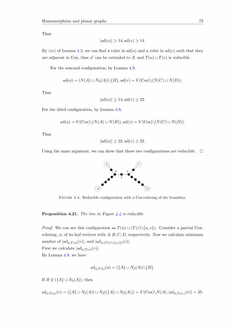
Homomorphism and planar graphs 73
Thus
|ad(u)| ≥ 14, ad(v) ≥ 14.
By (ix) of Lemma 4.5, we can find a color in ad(u) and a color in ad(v) such that they
are adjacent in Cox, thus φ′ can be extended to X and T (u) ∪ T (v) is reducible.
For the sencond configuration, by Lemma 4.9,
ad(u) = (N(A) ∪N3(A))\B, ad(v) = V (Cox)\(N(C) ∪N(D)).
Thus
|ad(u)| ≥ 14, ad(v) ≥ 22.
For the third configuration, by Lemma 4.9,
ad(u) = V (Cox)\(N(A) ∪N(B)), ad(v) = V (Cox)\(N(C) ∪N(D)).
Thus
|ad(u)| ≥ 22, ad(v) ≥ 22.
Using the same argument, we can show that these two configurations are reducible.
C
B D
A
u v
t
Figure 4.4: Reducible configuration with a Cox-coloring of the boundary.
Proposition 4.21. The tree in Figure 4.4 is reducible.
Proof. We can see this configuration as T (u) ∪ (T (v)\u, v). Consider a partial Cox-
coloring, φ, of its leaf vertices with A,B,C,D, respectively. Now we calculate minimum
number of |adφ,T (u)(v)|, and |adφ,(T (v)\u,v)(v)|.First we calculate |adφ,T (u)(v)|.By Lemma 4.9, we have
adφ,T (u)(u) = (A ∪N2(A))\B.
If B /∈ (A ∪N2(A)), then
adφ,T (u)(v) = (A ∪N2(A)) ∪N2((A ∪N2(A))) = V (Cox)\N(A), |adφ,T (x1)(v)| = 25.
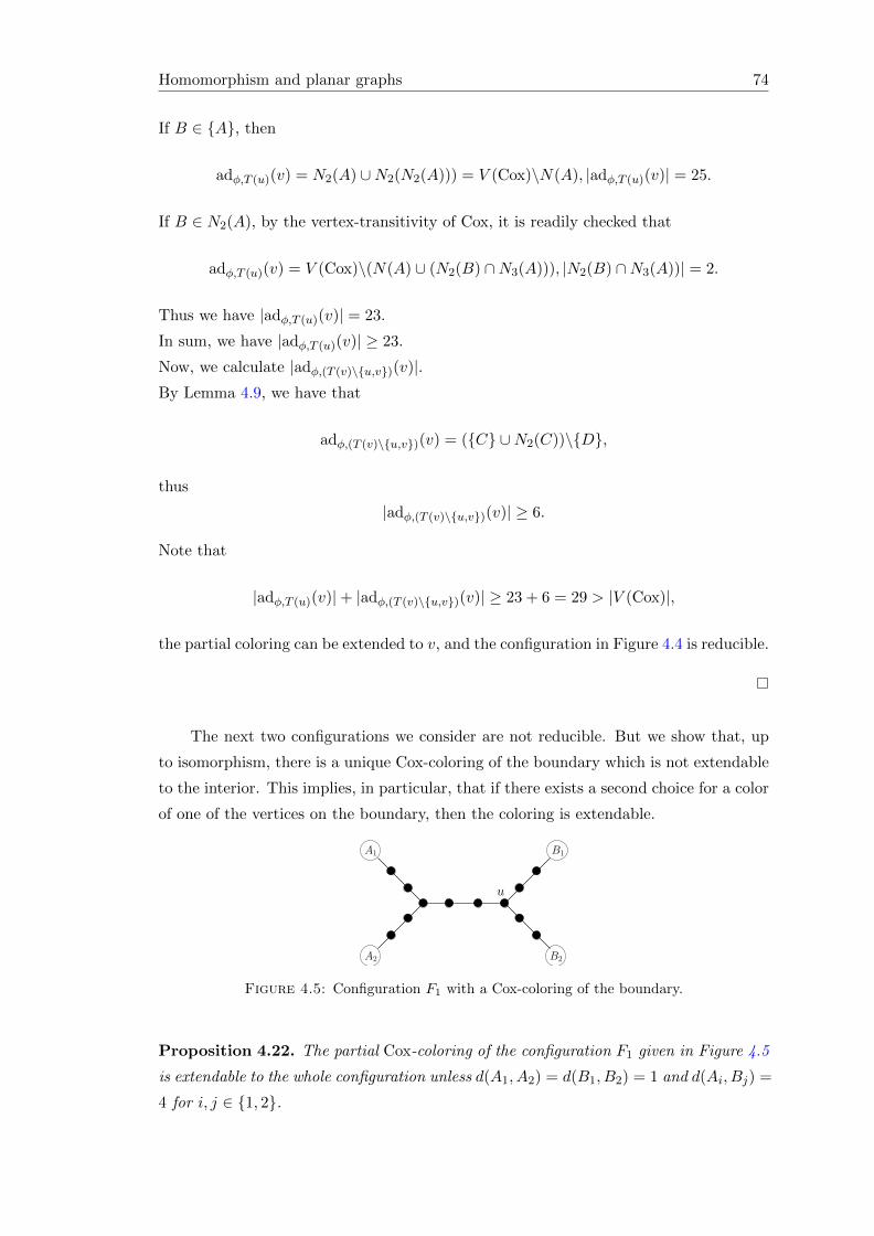
Homomorphism and planar graphs 74
If B ∈ A, then
adφ,T (u)(v) = N2(A) ∪N2(N2(A))) = V (Cox)\N(A), |adφ,T (u)(v)| = 25.
If B ∈ N2(A), by the vertex-transitivity of Cox, it is readily checked that
adφ,T (u)(v) = V (Cox)\(N(A) ∪ (N2(B) ∩N3(A))), |N2(B) ∩N3(A))| = 2.
Thus we have |adφ,T (u)(v)| = 23.
In sum, we have |adφ,T (u)(v)| ≥ 23.
Now, we calculate |adφ,(T (v)\u,v)(v)|.By Lemma 4.9, we have that
adφ,(T (v)\u,v)(v) = (C ∪N2(C))\D,
thus
|adφ,(T (v)\u,v)(v)| ≥ 6.
Note that
|adφ,T (u)(v)|+ |adφ,(T (v)\u,v)(v)| ≥ 23 + 6 = 29 > |V (Cox)|,
the partial coloring can be extended to v, and the configuration in Figure 4.4 is reducible.
The next two configurations we consider are not reducible. But we show that, up
to isomorphism, there is a unique Cox-coloring of the boundary which is not extendable
to the interior. This implies, in particular, that if there exists a second choice for a color
of one of the vertices on the boundary, then the coloring is extendable.
A1 B1
A2 B2
u
Figure 4.5: Configuration F1 with a Cox-coloring of the boundary.
Proposition 4.22. The partial Cox-coloring of the configuration F1 given in Figure 4.5
is extendable to the whole configuration unless d(A1, A2) = d(B1, B2) = 1 and d(Ai, Bj) =
4 for i, j ∈ 1, 2.

Homomorphism and planar graphs 75
Proof. Consider the T222 configuration whose boundary consists of the vertex u and the
two vertices colored with A1 and A2, respectively. If d(A1, A2) 6= 1, then by Lemma 4.15,
there are at least 27 choices of color for u which is extendable to the interior of this T222 .
On the other hand, by Lemma 4.14, there are at least 4 choices of color for u that
is extendable to a Cox-coloring of the partially colored 6-path connecting B1 and B2.
Thus, there are at least three common choices of color for u which is extendable on the
whole configuration.
If d(A1, A2) = 1, then, again by Lemma 4.15, there are exactly four non-extendable
choices of color for u for the considered T222 configuration. These particular four choices
are the neighbors of A1 and A2 distinct from A1 and A2. If any of the other 24 choices is
extendable on the B1-B2 path, then the coloring is extendable to the whole configuration.
Otherwise, by the proof of Lemma 4.14, we have d(B1, B2) = 1 and, furthermore,
d(Ai, Bj) = 4 for i, j ∈ 1, 2.
Corollary 4.23. For the configuration F1 of Figure 4.5, if the given partial Cox-coloring
is not extendable to the whole configuration, then A1 is uniquely determined by A2, B1
and B2.
Proof. Note that given an edge A1A2, the property d(Ai, Bj) = 4 for i, j ∈ 1, 2determines a unique edge in Cox, as shown in Lemma 4.5 (viii).
A1
B2
B1
A2
u
Figure 4.6: Configuration F2 with a Cox-coloring of the boundary.
Proposition 4.24. The partial Cox-coloring of the configuration F2 given in Figure 4.6
is extendable to the whole configuration unless d(A1, A2) = 1 and B1, B2 = A1, A2.
Proof. The proof is similar to that of the previous proposition. Again we consider the
possibilities on u. If d(A1, A2) 6= 1, then, by Lemma 4.15, there are at least 27 choices of
color for u that would be extendable on the part connecting to A1 and A2. Of these 27
vertices in Cox, at least two are neighbors of B1 and of these two, one is distinct from
B2. This color is an extendable choice.

Homomorphism and planar graphs 76
If d(A1, A2) = 1, then the four neighbors of A1 and A2, distinct from A1 and A2,
are the only choices for u that would make the coloring non-extendable on the left side.
If B1 /∈ A1, A2, then there are at least two neighbors of B1 whose assignments to u are
extendable on the left side of u, and at least one of these two is different from B2. Thus,
we may assume without loss of generality that B1 = A1. Then A2 is an extendable
choice for u unless B2 = A2.
Corollary 4.25. If the partial Cox-coloring of the configuration F2 given in Figure 4.6
is not extendable to the whole configuration, then A1 is uniquely determined by A2, B1
and B2.
4.4 Discharging and further reducible configurations
In this section, we will discharging technique to get a contradiction. Recall that X, our
minimal counterexample, is a 2-connected plane graph whose faces are all 17-cycles.
Since X is a plane graph, by Euler formula we have:
V − E + F = 2.
Here V,E, F are the number of vertices, edges and faces of X, respectively. Denote by
l(f) the length of face f . Then we have∑f
l(f) = 2E =∑v
d(v).
Thus
E − (V + F ) = −2⇒ 6E − 6(V + F ) = −12⇒ 3 · 2E − (∑v
6 +∑f
6) = −12.
If we choose two real numbers α and β satisfying α+ β = 3, then
(α+ β) · 2E − (∑v
6 +∑f
6) = −12.
Furthermore, we have
∑v
(α · d(v)− 6) +∑f
(β · l(f)− 6) = −12, (4.1)
Note that all the faces of X are 17-cycles, thus l(f) = 17 for all f ’s. If we set β = 617 ,
then β · l(f)− 6 = 0, and identity 4.1 reduces to
∑v
(45 · d(v)− 102) +∑f
0 = −204. (4.2)

Homomorphism and planar graphs 77
We give each vertex v of X the following initial charge:
w0(v) = 45 · d(v)− 102.
Note that the total sum of the initial charge∑
v∈V (X)w0(v) = −204 < 0. Since X is
2-connected, there is no 1-vertex, and it is easy to check that each 2-vertex has initial
charge −12, each 3-vertex has initial charge 33, each 4-vertex has initial charge 78. To
prove Theorem 4.3, we will redistribute the charges on the vertices so that at the final
step, the charge on each vertex is non-negative. This contradicts that the total charge
is negative and would disprove the existence of X. We will accomplish this through two
phases of discharging.
In the first phase, we will take care of vertices of degree 2.
Then, in the second phase, we design a discharging rule that would take care of all
negatively charged vertices after the first phase. We will then show that each configu-
ration which may lead to a vertex of negative charge is reducible. This would complete
our proof.
4.4.1 First phase of discharging
Here we use the following discharging rule:
(R1) For each pair x, y of weakly adjacent vertices in X with d(x) = 2 and d(y) ≥ 3, y
sends charge of 6 to x.
Let w1(v) denote the new charge at each vertex v.
If d(v) = 2 then v receives a total charge of 12 (6 from each of its weakly adjacent
3+-vertices), hence w1(v) = 0.
If d(v) = 3, then by Corollary 4.17, we have w1(v) ≥ 33− 6 · 6 = −3. Furthermore,
if dweak(v) 6= 6, then w1(v) ≥ 33− 5 · 6 = 3.
If d(v) = 4, we have w1(v) ≥ 78− 6 · 12 = 6 by Corollary 4.19.
If d(v) ≥ 5, we have w1(v) ≥ 45d(v) − 102 − 6 · 4d(v) = 21d(v) − 102 ≥ 3 by
Corollaries 4.11.
A vertex v of X is called poor if w1(v) < 0. As a consequence of Corollary 4.17, we
have the following characterization of poor vertices.
Proposition 4.26. A vertex v of X is poor if and only if d(v) = 3 and dweak(v) = 6.
Homomorphism and planar graphs 78
Corollary 4.17 also implies that for each poor vertex v, T (v) is one of the following
trees: T024 , T033 , T114 , T222 . Our aim is to seek charge for v from its closest leaf vertices
of T (v). Given a 3+-vertex x ∈ V (X), we say x supports v if:
(i) w1(x) > 0, and
(ii) x is a leaf vertex of T (v) on a shortest thread of T (v).
Note that each such thread has length at most 3. Furthermore, observe that v may
have more than one supporting vertex x.
4.4.2 Second phase of discharging
In this phase we try to increase the charge of all poor vertices. The discharging rule is
as follows:
(R2) Whenever y supports a poor vertex x, then y gives charge of 3 to x if d(x, y) = 1,
and charge of 1.5 to x if d(x, y) 6= 1.
Let w2(v) be the charge of an arbitrary vertex v after this phase. We will show that
w2(v) ≥ 0, for every vertex v of X.
Observe that the charge of each 2-vertex v remains the same, i.e. w2(v) = 0.
If v is a 5+-vertex, then by Corollary 4.11 we have
w1(v) ≥ w0(v)− 24d(v) = 21d(v)− 102 ≥ 3.
Furthermore, if v is a support for a vertex u, then the number of 2-vertices on the v-u
thread is at most two. Thus, if v supports r vertices then
w1(v) ≥ w0(v)− 6 · 4 · (d(v)− r)− 6 · 2r ≥ 21d(v)− 102 + 12r ≥ 3 + 12r.
This implies that
w2(v) ≥ 3 + 12r − 3r ≥ 3.
Now, assume v is a 4-vertex. By Corollary 4.19, unless T (v) = T0444 , we have
w1(v) ≥ 78− 6 · 11 = 12 and this clearly gives
w2(v) ≥ w1(v)− 4 · 3 ≥ 0.

Homomorphism and planar graphs 79
If T (v) = T0444 , then v supports at most one vertex, and therefore
w2(v) ≥ 78− 6 · 12− 3 = 3.
We are left to consider the case of a 3-vertex v, which supports at most 3 vertices.
If dweak(v) ≤ 4, then w2(v) ≥ w1(v)− 3 · 3 ≥ 33− 6 · 4− 9 = 0.
If dweak(v) = 5 and v support only one poor vertex, then w2(v) ≥ w1(v) − 3 ≥33− 6 · 5− 3 = 0.
The remaining two possibilities for v are as follows: either
(1) dweak(v) = 6, that means v is a poor vertex, or
(2) dweak(v) = 5 and v supports at least two poor vertices.
We will complete our proof by showing that:
(i) If v is a poor vertex, then either v has an adjacent supporting vertex or it has at
least two supporting vertices.
(ii) If d(v) = 3 and dweak(v) = 5, then when applying (R2) v sends total charge of at
most 3.
To prove (i), note that by Corollary 4.17 and Proposition 4.26, T (v) is one of the
following trees: T024 , T033 , T114 , T222 .
If T (v) is T024 or T033 , then v is adjacent to a 3+-vertex, say x. We claim that x
is the adjacent supporting vertex of v. To see this, suppose by contradiction x is poor.
Then, the union T (x)∪ T (v) must be one of the configurations of Figure 4.3. But these
are reducible configurations as shown in Proposition 4.20.
If T (v) is T114 , there are two 3+-vertices at distance 2 from v. It remains to prove
that neither of these two vertices is poor. By contradiction, suppose one of these two
3+-vertices, say x, is a poor vertex. Then T (x) must be one of T024 , T033 , T114 , T222 .
Since x and v are of distance 2, T (x) must be T114 . Since each face of X is a 17-cycle,
the union T (x) ∪ T (v) must be the configuration of Figure 4.4, which is shown to be
reducible in Proposition 4.21.
If T (v) is T222 , we prove that at most one vertex in N3(v) is poor. If x ∈ N3(v) is
a poor vertex, then T (x) must be either T222 or T024 . Then, the union F = T (v) ∪ T (x)
is, respectively, the configuration of Figure 4.5 or the configuration of Figure 4.6. Let y
be another vertex in N3(v). If y is also a poor vertex, then in X − Int(F ) the vertex y

Homomorphism and planar graphs 80
is an internal vertex of an induced 5-path P . Thus, by Lemma 4.13, there are at least
two choices for extending a Cox-coloring of (X − Int(F ))− Int(P ) to y, one of which is
extendable to a Cox-coloring of X by Corollary 4.23 or Corollary 4.25.
To prove (ii), we begin by observing that T (v) must be one of the configurations:
T014 , T023 , T113 , T122 .
If T (v) is T014 , we need to prove that v supports at most 1 poor vertex. Suppose to
the contrary that v supports 2 poor vertices, say x1 and x2, then x1 and x2 must be at
distance 1 and 2 to v, respectively. Assume without loss of generality that d(v, x1) = 1.
Since x1 is a poor vertex, T (x1) must be in T024 , T033. Then T (v)∪T (x1) has only two
such possible configurations, shown in Figure 4.7. In this figure, the vertex in square is
the poor vertex x1. We claim that each configuration of Figure 4.7 is reducible. To prove
this, we need to show that any partial Cox-coloring, φ, of the leaf vertices A,B,C,D
can be extended to the interior of T (v) ∪ T (x1).
For the first configuration, note that it can be seen as T (x1)∪(T (v)\x1), v is a leaf vertex
of T (x1) and a internal vertex of T (v)\x1. Now we calculate the minimum number of
|adφ,T (x1)(v)| and |adφ,T (v)\x1(v)|. By Lemma 4.9 we have that
adφ,T (x1)(x1) = (N(A) ∪N3(A))\B, adφ,T (x1)(v) = N((N(A) ∪N3(A))\B).
Using the vertex-transitivity of Cox, it is readily observed that
N((N(A) ∪N3(A))) = A ∪N2(A) ∪N3(A) ∪N4(A).
Note that if B /∈ (N(A) ∪N3(A)), then
adφ,T (x1)(v) = A ∪N2(A) ∪N3(A) ∪N4(A), |adφ,T (x1)(v)| = 25.
If B ∈ N(A), then
adφ,T (x1)(v) = N((N(A) ∪N3(A))\B) = N((N(A) ∪N3(A))), |adφ,T (x1)(v)| = 25.
If B ∈ N3(A), then
adφ,T (x1)(v) = N((N(A)∪N3(A))\B) = N((N(A)∪N3(A)))\C : C ∈ N3(A)∩N(B).
Note that |N3(A) ∩N(B)| = 1, then |adφ,T (x1)(v)| = 24.
In sum, |adφ,T (x1)(v)| ≥ 24.
By Lemma 4.9, we have
adφ,T (v)\x1(v) = (C ∪N2(C))\D,

Homomorphism and planar graphs 81
thus |adφ,T (v)\x1(v) ≥ 6|.
Note that
|adφ,T (x1)(v)|+ |adφ,T (v)\x1(v)| ≥ 30 > |V (Cox)|,
there is a good common choice for coloring v, which implies that φ can be extended to
the interior of T (v) ∪ T (x1) and the first configuration is reducible.
For the second configuration, by the same method and notations and by Lemma 4.9,
we have that
adφ,T (x1)(x1) = V (Cox)\N(A) ∪N(B).
Note that,
adφ,T (x1)(v) = N(adφ,T (x1)(x1)),
a vertex C is in adφ,T (x1)(v) if and only if N(C) * N(A) ∪N(B). By (x) of Lemma
4.5, if C /∈ A,B, then |N(C) ∩N(A)| ≤ 1 and |N(C) ∩N(B)| ≤ 1, thus
|N(C) ∩ (N(A) ∪N(B))| ≤ 2,
which implies that C ∈ adφ,T (x1)(v). We have adφ,T (x1)(v) = V (Cox)\A,B and
|adφ,T (x1)(v)| ≥ 26. Note that |adφ,T (v)\x1(v) ≥ 6|, we have
|adφ,T (x1)(v)|+ |adφ,T (v)\x1(v)| ≥ 32 > |V (Cox)|.
This implies that the second configuration is reducible.
CC
B
A
B D
A
D
v v|ad(v)| > 24 |ad(v)| > 6 |ad(v)| > 26 |ad(v)| > 6
Figure 4.7: Local configurations of a center of T014
supporting two poor vertices.
If T (v) is T023 , using the Figure 4.8, a similar argument is applied.
If T (v) is T113 , then v is a support of at most two poor vertices (leave vertices at
distance 2 to v) to each of which it may send charge of 1.5. Hence, in the second phase
v gives as support at most charge of +3.

Homomorphism and planar graphs 82
C CA
BD D
A
vv|ad(v)| > 24 |ad(v)| > 26 |ad(v)| > 12|ad(v)| > 12
B
Figure 4.8: Local configurations of a center of T023
supporting two poor vertices.
Finally, assume that T (v) is T122 . By (R2), v gives each of its supported vertex
of charge 1.5. Note that w1(v) = 3, if w2(v) < 0, v supports 3 poor vertices, namely
three leave vertices of T (v), denoted x1, x2, x3. Assume without loss of generality that
d(v, x1) = 2, d(v, x2) = d(v, x3) = 3. Note that T (xi) ∈ T024 , T033 , T114 , T222, T (x1)
must be T114 , T (x2) and T (x3) must be T222 . In this case, we have a unique local
configuration, given in Figure 4.9, we can see it by T (x1)∪T (x2)∪Pvx3 , here Pvx3 is the
thread connecting v and x3. We claim that T (x1)∪T (x2)∪Pvx3 is reducible. To see this,
consider a partial Cox-coloring, φ, of its leaf vertices with A,B,C,D, F , respectively.
Now we calculate minimum number of |adφ,T (x1)(v)|, |adφ,T (x2)(v)| and |adφ,Pvx3(v)|.
First we calculate |adφ,T (x1)(v)|.By Lemma 4.9, we have
adφ,T (x1)(x1) = (A ∪N2(A))\B.
If B /∈ (A ∪N2(A)), then
adφ,T (x1)(v) = (A∪N2(A))∪N2((A∪N2(A))) = V (Cox)\N(A), |adφ,T (x1)(v)| = 25.
If B ∈ A, then
adφ,T (x1)(v) = N2(A) ∪N2(N2(A))) = V (Cox)\N(A), |adφ,T (x1)(v)| = 25.
If B ∈ N2(A), by the vertex-transitivity of Cox, it is readily checked that
adφ,T (x1)(v) = V (Cox)\(N(A) ∪ (N2(B) ∩N3(A))),
and |N(B) ∩N3(A))| = 2. We have |adφ,T (x1)(v)| = 23.
In sum, we have |adφ,T (x1)(v)| ≥ 23.
By Lemma 4.15, |adφ,T (x2)(v)| ≥ 28− 4 = 24.

Homomorphism and planar graphs 83
By Lemma 4.9, |adφ,Pvx3(v)| ≥ 15. It is easy to check that
|adφ,T (x1)(v) ∩ adφ,T (x2)(v) ∩ adφ,Pvx3(v)| ≥ 6.
Thus there is a common choice for v.
C
D
A
B
F
v|ad(v)| > 23
|ad(v)| >
24
|ad(v)| >
15
Figure 4.9: Local configuration of a center of T122
supporting three poor vertices.
4.5 Concluding remarks and further work
We have shown in this paper that one may use the existence of a combinatorial design
to propose answer for special cases of the Problem 4.1. Our primary concern in this
paper was the case r = 5 and k = 3 of this question and we proposed an answer using
the Fano plane. At a 2011 summer workshop in Prague, Peter Cameron has proposed
a similar conjecture for the case of r = 7 and k = 5 based on the existence of a unique
Steiner quintuple system of order 11.
The condition of odd-girth 17 was used only when applying Euler formula, indeed
each of the 15 reducible configurations we used in our proof is a tree. Thus if X is a min-
imal graph which admits no homomorphism to Cox (i.e., every proper subgraph admits
a homomorphism to Cox), then X does not contain any of these reducible configura-
tions. We believe that with a larger set of reducible trees and together with cumbersome
discharging steps we can improve the result for odd-girth 15. However, it seems that
to prove the conjecture using the discharging technique, if possible at all, one has to
consider reducible configurations that involve cycles.

Chapter 5
Locating any two vertices on
Hamiltonian cycles
In this chapter we give a proof of Conjecture 1.47 ( Enomoto’s conjecture ) for graphs
of sufficiently large order. We recall Enomoto’s conjecture here.
Conjecture 5.1. [39] If G is a graph of order n ≥ 3 and δ(G) ≥ n2 +1, then for any pair
of vertices x, y in G, there is a Hamiltonian cycle C of G such that distC(x, y) = bn2 c.
Our main result is the Theorem 1.52. We state again this theorem here.
Theorem 5.2. [48] There exists a positive integer n0 such that for all n ≥ n0, if G is
a graph of order n with δ(G) ≥ n2 + 1, then for any pair of vertices x, y in G, there is a
Hamiltonian cycle C of G such that distC(x, y) = bn2 c.
The main tools of our proof are Regularity Lemma of Szemeredi and Blow-up
Lemma of Komlos et al. In section 5.1, we will introduce these lemmas and some
applications of them.
In this chapter, we use a new notation of degree of a vertex. For any vertex v of G
and a subset X of V (G), we denote the degree of v in G by degG(v) and the degree of
v in X by degG(v,X) (if no ambiguity arises, we denote them by deg(v) and deg(v,X)
respectively).
5.1 Regularity Lemma and Blow-up Lemma
In this section we introduce Regularity Lemma and Blow-up Lemma.
84

Locating vertices on Hamiltonian cycles 85
The Regularity Lemma, Szemeredi’s Regularity Lemma [96], is a powerful tool of
graph theory. It was invented as an auxiliary lemma in the proof of the famous conjecture
of Erdos and Turan [27] which states that sequences of integers of positive upper density
must always contain long arithmetic progressions.
To introduce Regularity Lemma and Blow-up Lemma, we first give some definitions
about the regular pairs and some related results.
5.1.1 Regular pairs and related properties
Given a graph G, let X and Y be two disjoint sets of vertices of G. In particular, G
could be a bipartite graph with vertex classes X and Y . We define the density, d(X,Y ),
of the pair (X,Y ) as the ratio
d(X,Y ) :=eG(X,Y )
|X||Y |,
here eG(X,Y ) is defined to be the number of edges in G with one end vertex in X and
the other in Y , if no ambiguity arises, we write e(X,Y ) instead of eG(X,Y ).
Let ε > 0. Given two disjoint vertex sets X ⊆ V (G), Y ⊆ V (G) we say the pair
(X,Y ) is ε-regular if for every A ⊆ X and B ⊆ Y such that |A| > ε|X| and |B| > ε|Y |we have
|d(A,B)− d(X,Y )| < ε.
From the definition we can see that the edges between an ε-regular pair are dis-
tributed fairly uniformly. Moreover, most of vertices of one part have a fairly large
number of neighbors in the other part, we can see this from the following lemma.
Lemma 5.3. [61] Let (A,B) be an ε-regular pair of density d and Y ⊆ B such that
|Y | > ε|B|. Then all but at most ε|A| vertices in A have more than (d− ε)|Y | neighbors
in Y .
The following lemma says that subgraphs of regular pairs with reasonable size are
also regular.
Lemma 5.4 (Slicing Lemma). [61] Let α > ε > 0 and ε′ := max εα , 2ε. Let (A,B) be
an ε-regular pair with density d. Suppose A′ ⊆ A such that |A′| ≥ α|A|, and B′ ⊆ B such
that |B′| ≥ α|B|. Then (A′, B′) is an ε′-regular pair with density d′ such that |d′−d| < ε.
The Slicing Lemma tells us that not too small subgraphs of an ε-regular pair are also
regular with density close to that of the original pair. Sometimes, in some situations,

Locating vertices on Hamiltonian cycles 86
we only consider some of the vertices in an ε-regular pair, we hope that as many as
possible the properties of the original pair do not just disappear. For this, we consider
an application of the Slicing Lemma which links the notation of regularity to that of
super-regularity.
Given a graph G and disjoint vertex sets X,Y ⊆ V (G) let ε, δ > 0, the pair
(X,Y ) is (ε, δ)-super-regular if it is ε-regular, and degY (x) > δ|Y | for all x ∈ X and
degX(y) > δ|X| for all y ∈ Y .
From next lemma we can see that: given a regular pair we can approximate it by a
super-regular pair.
Lemma 5.5. [98] If (X,Y ) is an ε-regular pair with density d in a graph G (where
0 < ε < 13 ), then there exists A′ ⊆ A,B′ ⊆ B with |A′| ≥ (1−ε)|A| and |B′| ≥ (1−ε)|B|,
such that (A′, B′) is a (2ε, d− 3ε)-super-regular pair.
For a bipartite graph G = X ∪Y , let δ(X,Y ) := minx∈XdegG(x, Y ). We can say that
a bipartite graph with very large minimum degree has a super-regular pair.
Lemma 5.6. [16] Given 0 < ρ < 1, let G = X ∪ Y be a bipartite graph such that
δ(X,Y ) ≥ (1 − ρ)|Y | and δ(Y,X) ≥ (1 − ρ)|X|. Then (X,Y ) is (√ρ, 1 − ρ)-super-
regular.
5.1.2 Regularity Lemma and Blow-up Lemma
Now we introduce Szemeredi’s Regularity Lemma.
First we state the original version of the Regularity Lemma.
Theorem 5.7. [96] For every ε > 0 and every m ∈ N, there exist two integers
M(ε,m) and N(ε,m) such that every graph G of order n ≥ N(ε,m) admits a parti-
tion V0, V1, . . . , Vk of V (G) such that:
(i) m ≤ k ≤M ,
(ii) 0 ≤ |V0| ≤ ε|G|,(iii) |V1| = |V2| = . . . = |Vk|,(iv) all but at most εk2 of the pairs (Vi, Vj) with 1 ≤ i < j ≤ k are ε-regular.
The classes Vi’s are usually called clusters and the partition described is called an
ε-regular partition. Note that V0 may be empty, we call it an exceptional set because its
role is purely technical: to make possible that all other clusters have exactly the same
cardinality. The role of m is to make the clusters Vi’s sufficiently small, so that the
number of edges inside those clusters are negligible.

Locating vertices on Hamiltonian cycles 87
In the applications of the original Regularity Lemma, one usually, in the first step,
apply the lemma to create a regular partition, then in the second step, get rid of all edges
except the edges between regular pairs of high enough densities, the leftover graphs still
contain most of the original edges, and much easier to handle. This process leads the
degree form of the Regularity Lemma, which is more applicable.
Lemma 5.8 (Regularity Lemma-Degree Form). For every ε > 0 and every integer m0
there is an M0 = M0(ε,m0) such that if G = (V,E) is any graph on at least M0 vertices
and d ∈ [0, 1] is any real number, then there is a partition of the vertex set V into l + 1
clusters V0, V1, ..., Vl, and there is a subgraph G′
= (V,E′) with the following properties:
(1) m0 ≤ l ≤M0;
(2) |V0| ≤ ε|V | for 0 ≤ i ≤ l, and |V1| = |V2| = · · · = |Vl| = L;
(3) degG′ (v) > degG(v)− (d+ ε)|V | for all v ∈ V ;
(4) G′[Vi] = ∅ (i.e. Vi is an independent set in G
′) for all i;
(5) each pair (Vi, Vj), 1 ≤ i < j ≤ l, is ε-regular, each with a density either 0 or at least
d.
We refer to [61] for more versions of the Regularity Lemma.
How to apply the Regularity Lemma? In the earlier time, many applications of
the Regularity Lemma are concerned with embedding and packing problem, there are
basically three steps to apply the lemma (suppose we try to embed a graph H into G).
Step 1. Apply Theorem 5.8 to G with suitable parameters ε and d, and construct a
reduced graph which is defined as following:
Let G be a graph and V1, V2, . . . , Vr a partition of V (G). Given two parameters ε > 0
and d ∈ [0, 1), we define the reduced graph R of G as follows: its vertices are the clusters
V1, V2, . . . , Vr and there exists an edge between Vi and Vj precisely when (Vi, Vj) is ε-
regular with density more than d. Let R(t) be a graph obtained from R by replacing
the edges of R by copies of Kt,t.
Step 2. Find a graph containing H in R(t).
Step 3. Apply the Key Lemma to imply that H ⊆ G as required. Key Lemma is given
in [61].
Theorem 5.9 (Key Lemma). [61] Given d > ε > 0, a graph R , and a positive integer
m, let us construct a graph G by replacing every vertex of R by m vertices, and replacing
the edges of R with ε-regular pairs of density at least d. Let R(t) be a graph obtained
from R by replacing the edges of R by copies of Kt,t. Let H be a subgraph of R(t) with
h vertices and maximum degree ∆ > 0, and let δ := d− ε and ε0 := δ∆
2+∆ . If ε ≤ ε0 and
t− 1 ≤ ε0m, then H ⊆ G.

Locating vertices on Hamiltonian cycles 88
Remark: The order of R plays no role here. The order of H is smaller than the
order of G.
An application of the Regularity Lemma is about embedding spanning graphs into
dense graphs. Some of the proofs use a powerful tool — Blow-up Lemma. Basically, it
sees the super-regular pairs as complete bipartite graphs.
Theorem 5.10 (Blow-up Lemma [59]). Given a graph R of order r and positive param-
eters δ,∆, there exists an ε > 0 such that the following holds.
Let n1, n2, . . . , nr be arbitrarily positive integers and let us replace the vertices of R with
pairwise disjoint sets V1, V2, . . . , Vr of sizes n1, n2, . . . , nr (respectively, blowing up). We
construct two graphs on the same vertex set V = ∪ri=1Vi. The first graph R is obtained
by replacing each edge vivj of R with the complete bipartite graphs between the corre-
sponding vertex sets Vi and Vj. A sparser graph G is constructed by replacing each edge
vivj of R with an (ε, δ)-super-regular pair between the corresponding vertex sets Vi and
Vj. If a graph H with ∆(H) ≤ ∆ is embeddable into R, then it is already embedded into
G.
Note that for embedding spanning subgraphs, one needs all degrees of the host
graphs are large enough, that’s why we use super-regular pairs while not the regular
pairs when we construct the second graph G in the above theorem. In total, while Key
Lemma plays a role in embedding smaller graphs H into G, Blow-up Lemma plays the
role in embedding spanning graphs H into G.
The following special case of the Blow-up Lemma, Bipartite Version of Blow-up
Lemma, which also restricts the mappings of a smaller number of vertices.
Lemma 5.11 (Blow-up Lemma-Bipartite Version [59]). For every δ,∆, c > 0, there
exists an ε = ε(δ,∆, c) > 0 and α = α(δ,∆, c) > 0 such that the following holds. Let
(X,Y ) be an (ε, δ)-super-regular pair with |X| = |Y | = N . If a bipartite graph H with
∆(H) ≤ ∆ can be embedded in KN,N by a function φ, then H can be embedded in (X,Y ).
Moreover, in each φ−1(X) and φ−1(Y ), fix at most αN special vertices z, each of which
is equipped with a subset Sz of X or Y of size at least cN . The embedding of H into
(X,Y ) exists even if we restrict the image of z to be Sz for all special vertices z.
Actually, the following special case of the Blow-up Lemma is frequently used in this
thesis.
Lemma 5.12. For every δ > 0 there are εBL = εBL(δ), nBL = nBL(δ) > 0 such that if
ε ≤ εBL and N ≥ nBL, G = (X,Y ) is an (ε, δ)-super-regular pair with |X| = |Y | = N ,
x1, x2 ∈ X (x1 6= x2), y1, y2 ∈ Y (y1 6= y2) and li is an even integer with 4 ≤ li ≤ 2N−4

Locating vertices on Hamiltonian cycles 89
(i = 1, 2), l1 + l2 = 2N , then there are two vertex-disjoint paths P1 and P2 in G such
that the end vertices of Pi are xi, yi and |V (Pi)| = li (i = 1, 2).
Proof. Let X∗ = X −x1, x2, Y ∗ = Y −y1, y2 and H = H1 ∪H2 be the union of two
vertex-disjoint paths H1, H2 satisfied |V (Hi)| = li − 2 (i = 1, 2). It is not hard to see
that H can be embedded in KN−2,N−2. By Slicing Lemma, we know that (X∗, Y ∗) is
also a super-regular pair. Fix the end vertices of H1 and H2 to be the special vertices.
For Hi, one of its end vertices is equipped with the neighbor set of xi and the other end
vertex is equipped with the neighbor set of yi (i = 1, 2). By Lemma 5.11, H can be
embedded in (X∗, Y ∗) satisfying the restrictions of the special vertices. Since one of the
end vertices of Hi is a neighbor of xi and the other end vertex of Hi is a neighbor of yi,
we can extend Hi to a path Pi with end vertices xi and yi (i = 1, 2). Then P1 ∪ P2 is a
spanning subgraph of G and |V (Pi)| = li (i = 1, 2).
5.1.3 Some applications of Regularity Lemma
Early applications of Regularity Lemma include Ramsey-Turan theory, generalized ran-
dom graphs, building packing with small graphs, et. al.
In 1992, Alon and Yuster [2] proved the following theorem:
Theorem 5.13. [2] For any α > 0 and graph H, there is an n0 such that
n ≥ n0, δ(Gn) >
(1− 1
χ(H)+ α
)n
imply that there are (1−α)n|V (H)| vertex-disjoint subgraphs, each being isomorphic to H, in
Gn.
In 1998, Komlos, Sarkozy and Szemeredi [60] proved Posa-Seymour conjecture for
graphs of large enough orders.
Theorem 5.14. [60] For any ε > 0 and any positive integer k, there is an n0 such that
if G has order n ≥ n0 and minimum degree at least(
1− 1k+1 + ε
)n, then G contains
the k-th power of a Hamiltonian cycle.
Note that in Theorem 5.14, the k-th power of a Hamiltonian graph H is the graph
obtained from H by joining every pair of vertices with distance at most k in H.
For some other early applications of Regularity Lemma we refer to [61].
Recently many long-standing conjectures about Hamiltonian problems are proved
or partially proved by using the Regularity Lemma.

Locating vertices on Hamiltonian cycles 90
In 1971, Nash-Williams [87] conjectured that:
Conjecture 5.15. [87] Let G be a d-regular graph on at most 2d vertices. Then G
contains bd2c edge-disjoint Hamiltonian cycles.
In 2012, Christofides, Kuhn and Osthus [18] proved an approximate version of
Conjecture 5.15.
Theorem 5.16. [18] For every α > 0 there is an integer n0 so that every d-regular graph
on n ≥ n0 vertices with d ≥(
12 + α
)n contains at least d−αn
2 edge-disjoint Hamiltonian
cycles.
In [22], Csaba et al. proved the following theorems.
Theorem 5.17 (1-factorization conjecture). [22] There exists an n0 ∈ N such that the
following holds. Let n,D ∈ N be such that n ≥ n0 is even and D ≥ 2dn4 e − 1. Then
every D-regular graph G on n vertices has a 1-factorization. Equivalently, χ′(G) = D.
Here a 1-factorization of a graph G consists of a set of edge-disjoint perfect match-
ings covering all edges of G.
Theorem 5.18 (Hamilton decomposition conjecture). [22] There exists an n0 ∈ N such
that the following holds. Let n,D ∈ N be such that n ≥ n0 and D ≥ bn2 c. Then every
D-regular graph G on n vertices has a decomposition into Hamilton cycles and at most
one perfect matching.
For more progress on F -packing, Hamiltonian problems and tree embedding, we
refer to [62]. For the progress on Hamiltonian cycles in directed graphs, oriented graphs
and tournaments, we refer to [63]
5.2 Overview of the proof of Theorem 5.2
In our proof for Theorem 5.2 we will use the Regularity Lemma and Blow-up Lemma as
many other studies (see [16], [91] for some similar ideas).
For proving Theorem 5.2, we only need to consider the graphs of even order. For
a graph G of odd order n, we choose one vertex v in G which is not either of the two
vertices x, y, then the minimum degree of graph G∗ = G−v is at least dn2 e = n−12 + 1.
Since G∗ is a graph of even order, by assumption we can locate x, y with distance n−12
on a Hamiltonian cycle C∗ of G∗. By the degree condition of v in G, there exsit two

Locating vertices on Hamiltonian cycles 91
consecutive vertices u1, u2 on C∗ which are adjacent to v. Replacing the edge u1u2 on
C∗ by the 2-path u1vu2, we obtain a Hamiltonian cycle of G in which x, y have distancen−1
2 = bn2 c.
Now let us consider a graph G of even order n with
δ(G) ≥ n
2+ 1. (5.1)
We assume that n is sufficiently large and we fix the following sequence of parame-
ters,
0 < ε d α 1. (5.2)
Here a b means a is sufficiently small compared to b. For simplicity, we don’t specify
their dependencies in the proof, although we could.
A balanced partition of V (G) into V1 and V2 is a partition of V (G) = V1 ∪ V2 such
that |V1| = |V2| = n2 . We define two extremal cases as follows.
Extremal Case 1: There exists a balanced partition of V (G) into V1 and V2 such
that the density d(V1, V2) ≥ 1− α.
Extremal Case 2: There exists a balanced partition of V (G) into V1 and V2 such
that the density d(V1, V2) ≤ α.
The proof of Theorem 5.2 will be divided into two parts: the non-extremal case
part in Section 5.3 and the extremal cases part in Section 5.4.
For the non-extremal case, the proof consists of the following four steps.
Step 1: We apply the Regularity Lemma to the graph G and find a Hamiltonian
cycle in the reduced graph.
Step 2: By the Hamiltonian cycle in the reduced graph, we obtain a perfect matching
of the reduced graph and we define the pairs of clusters according to the matching. We
construct some paths to connect the clusters in different pairs.
Step 3: We use all the vertices in V0 to extend those paths constructed in step 2.
Step 4: We apply Lemma 5.12 in each pair of clusters to finally construct a Hamil-
tonian cycle in G. And we make sure that x, y have distance bn2 c on this cycle.
Indeed, due to the parity of n2 , our proof will have some cases discussions.
For two extremal cases, we will prove a structure lemma for each case to make the
partition of V (G) more helpful for the proof (Lemma 5.27 and Lemma 5.29). By Lemma

Locating vertices on Hamiltonian cycles 92
5.27, a graph in extremal case 1 is like a balanced bipartite graph except some special
vertices, then we will use Lemma 5.12 to construct our desired Hamiltonian cycle. And
by Lemma 5.29, a graph in extremal case 2 is like a union of two high minimum degree
subgraphs except some special vertices. All these two extremal cases will have some
sub-case discussions based on the parity of n2 .
5.3 Non-extremal case
5.3.1 Applying the Regularity Lemma
Let G be a graph which is not either of the extremal cases and the vertices x, y have
been chosen. We apply the Regularity Lemma (in this thesis we always refer to Theorem
5.8) to G with parameter ε and d as in equation 5.2. We get a partition of V (G) into
l+ 1 clusters V0, V1, V2, ..., Vl. Assume that l is even, if not, we move the vertices of one
of the clusters into V0 (also denote it by V0) to make l be an even number. Now, by (2)
of Theorem 5.8, we have |V0| ≤ 2εn and
(1− 2ε)n ≤ lN ≤ n. (5.3)
Let k := l2 .
We define the reduced graph R based on the clusters V1, . . . , Vl (a partition of
V (G) \ V0): the vertices of R are r1, r2, ..., rl, and there is an edge between ri and rj
if the pair (Vi, Vj) is ε-regular in G′
with density at least d. If no ambiguity arises, we
won’t distinguish the cluster and its corresponding vertex in R.
The following claim shows that R inherits the minimum degree condition.
Claim 5.19. δ(R) ≥ (12 − 2d)l.
Proof. For any cluster Vi (1 ≤ i ≤ l), the neighbors of v ∈ Vi in G′
can only be in V0 and
in the clusters which are neighbors of Vi in R. Consider the sum of degrees of vertices
in Vi, in one hand,
(n
2+ 1− (d+ ε)n)L ≤
∑v∈Vi
degG′ (v);
in the other hand, ∑v∈Vi
degG′ (v) ≤ 2εnL+ degR(ri)L2.
Thus degR(ri) ≥ (12 − d− 3ε)nL > (1
2 − 2d)l provided 3ε < d.

Locating vertices on Hamiltonian cycles 93
The assumption that G is not either of the extremal cases leads the following claim.
Claim 5.20. G is a graph which is not either of the extremal cases, then
(1) the independence number of R is less than (12 − 8d)l,
(2) R contains no two disjoint subsets R1, R2 of size at least (12 − 6d)l such that
eR(R1, R2) = 0.
Proof. (1) Suppose to the contrary that R contains an independent set R1 of size (12 −
8d)l. We will show that G is in the Extremal Case 1 with parameter α. Let A = ∪ri∈R1Vi
and B = V (G)−A. By equation 5.3,(1
2− 9d
)n ≤
(1
2− 8d
)lL = |R1|L = |A| <
(1
2− 2d
)n.
For each x ∈ A, by (3) of Theorem 5.8,
degG(x,A) ≤ degG′(x,A) + (d+ ε)n < 2dn,
then we have
degG(x,B) >n
2− 2dn =
(1
2− 2d
)n.
Hence,
eG(A,B) >
(1
2− 9d
)n ·(
1
2− 2d
)n >
(1
4− 11
2d
)n2.
Now move at most 9dn vertices from B to A such that A and B are of size n2 . We still
have
eG(A,B) >
(1
4− 11
2d
)n2 − 9dn · n
2=
(1
4− 10d
)n2 = (1− 40d)
(n2
)2.
By specializing 40d ≤ α, we get that G is in the Extremal Case with parameter α.
(2) Suppose to the contrary that R contains two disjoint subsets R1, R2 of size(12 − 6d
)l such that eR(R1, R2) = 0. We will show that G is in the Extremal Case 2
with parameter α. Let A = ∪ri∈R1Vi and B = ∪ri∈R2Vi. Since eR(R1, R2) = 0, we have
eG′(A,B) = 0. By (3) of Theorem 5.8, we have |E(G)| ≤ |E(G′)|+ dn2, we have
eG(A,B) ≤ eG′(A,B) + dn2 = dn2.
Note that
|A| = |R1|L =
(1
2− 6d
)lL >
(1
2− 7d
)n,
and
|B| = |R2|L =
(1
2− 6d
)lL >
(1
2− 7d
)n.

Locating vertices on Hamiltonian cycles 94
By adding at most 7dn vertices to each of A and B, we obtain two subsets of size n2 and
still name them as A and B, respectively. Then,
eG(A,B) ≤ dn2 + 2 · (7dn)(n
2
)= 8dn2,
which in turn shows that the density
dG(A,B) =eG(A,B)(
n2
)2 ≤ 32d.
Since α > 32d, we obtain that G is in the Extremal Case 2 with parameter α.
Note that Claim 5.20 shows that there exists an upper bound of the independence
number of R. The proof of this lemma is similar to the proof of Claim 4.5 in [16],
By Claim 5.20, we can say that R is Hamiltonian. To prove this, we need a theorem
of Nash-Williams.
Theorem 5.21. [85] Let G be a 2-connected graph of order n. If minimum degree
δ(G) ≥ maxn+23 , α(G), here α(G) is the independence number of G, then G contains
a Hamiltonian cycle.
Claim 5.22. R is a Hamiltonian graph.
Proof. By δ(R) ≥ (12 − 2d)l and Lemma 5.20, we can say that δ(R) ≥ max l+2
3 , α(R).Now we only need to prove that R is a 2-connected graph.
Actually, we can show that R is dl-connected. To the contrary suppose that there
exists a vertex cut S in R with |S| < dl. Let X and Y be two components in R−S. Since
δ(R) ≥ (12−2d)l, the size of X and Y should be more than (1
2−3d)l. And eG(X,Y ) = ∅,which is impossible by Lemma 5.20. So R is dl-connected.
Since n ≤ Ll + 2εn ≤ (l + 2)εn, l ≥ 1ε − 2. Suppose 5ε ≤ d, we can get l ≥ 3
d . So
dl ≥ 3 which leads to the end of the proof.
There are also some similar arguments in [16].
5.3.2 Constructing paths to connect clusters
We say that a vertex v is friendly to a cluster X, denoted v ∼ X, if degG(v,X) ≥(d − ε)|X|. Moreover, given an ε-regular pair (X,Y ) of clusters and a subset Y
′ ⊆ Y ,
we say that a vertex v ∈ X is friendly to Y′, if deg(x, Y
′) ≥ (d − ε)|Y ′ |. Actually by
Lemma 5.3, at most ε|X| vertices of X are not friendly to Y′
whenever |Y ′ | > ε|Y |.

Locating vertices on Hamiltonian cycles 95
Claim 5.23. Every vertex v ∈ V (G) is friendly to at least (12 − 2d)l clusters.
Proof. Assume for a contradiction that there are less than (12 − 2d)l friendly clusters for
v. Then
degG(v) ≤ (1
2− 2d)lL+ (d− ε)Ll + 2εn ≤ (
1
2− d+ 2ε)n <
n
2,
provided that 2ε < d, which is a contradiction to equation 5.1.
If two clusters X and Y are a regular pair, we denote this relation by X ∼ Y . Given
two vertices u, v ∈ V (G), a u, v-chain of length 2s with distinct clusters A1, B1, ..., As, Bs
is u ∼ A1 ∼ B1 ∼ · · · ∼ As ∼ Bs ∼ v and Aj , Bj = Xi, Yi for some 1 ≤ i ≤ k. We
have the following claim. There are also some similar discussions in [16], but we give
the claim with a different bound on the number of the chains.
Claim 5.24. Let L be a list of at most 2εn pairs of vertices of G. For each pair
u, v ∈ L, we can find u, v-chains of length two or four such that every cluster is used
in at most d10L chains.
Proof. We deal with one pair in L at each step. Suppose we have found the desired
chains for s < 2εn pairs such that no cluster is used in more than d10L chains. Let O be
the set of clusters which are used d10L times.
We have a bound on the cardinality of O,
d
10L|O| ≤ 4s ≤ 8εn ≤ 8ε
2kL
1− 2ε.
So |O| ≤ 160εk(1−2ε)d ≤
160εld ≤ dl, provided d2 ≥ 160ε.
Now consider a new pair u, v in L, we try to find a u, v-chain of length at most
four such that every cluster is used in at most d10L chains. Let U be the set of clusters
which are friendly to u and not in O. Similarly, let V be the set of clusters which are
friendly to v and not in O. Let P (U) and P (V) be the set of partners of clusters in Uand V, respectively. It is easy to see that |U| = |P (U)| and |V| = |P (V)|. Moreover,
since |O| ≤ dl, by Claim 5.23, we know that |U| = |P (U)| ≥ (12−3d)l and |V| = |P (V)| ≥
(12 − 3d)l. Denote by R1 the set of vertices in R which are corresponding to the clusters
in P (U), and by R2 the set of vertices in R which are corresponding to the clusters in
P (V).

Locating vertices on Hamiltonian cycles 96
First, we claim that eR(R1, R2) 6= 0. Suppose to the contrary that eR(R1, R2) = 0.
If R1 ∩R2 = ∅, Then R1 and R2 are disjoint and eR(R1, R2) = 0. Since |R1| = |P (U)| ≥(1
2 − 3d)l and |R2| = |P (V)| ≥ (12 − 3d)l, we get a contradiction to Claim 5.20.
If there exists a vertex x ∈ R1∩R2, then degR(x) ≥ (12−2d)l. Since eR(R1, R2) = 0,
x is not adjacent to any vertex in R1 ∪ R2. Thus |R1 ∪ R2| ≤ (12 + 2d)l. Since |R1| ≥
(12 − 3d)l and |R2| ≥ (1
2 − 3d)l, |R1 ∩R2| ≥ (12 − 8d)l. R1 ∩R2 is an independent set in
R, which is a contradiction to Claim 5.20.
Now eR(R1, R2) 6= 0, that means there exist a cluster in P (U), say A, and a cluster
in P (V), say B, such that A ∼ B. Denote the partner of A in U by A′ and the
partner of B in V by B′. If A,A′, B,B′ are mutually distinct, then we get a u, v-chain
u ∼ A′ ∼ A ∼ B ∼ B′ ∼ v of length four. If A′ = B or A = B′, we get a u, v-chain
u ∼ B ∼ B′ ∼ v or u ∼ A′ ∼ A ∼ v of length two, respectively.
Continue this process until there is no pair in L is left.
Let CR be a Hamiltonian cycle in R. We choose two distinct clusters X, Y which
are as close as possible on CR such that x is friendly to Y and y is friendly to X.
Claim 5.25. We can choose distinct clusters X and Y such that x is friendly to Y , y
is friendly to X and distCR(X,Y ) ≤ 3dl.
Proof. Let X be the the family of friendly clusters for x and Y be the the family of
friendly clusters for y. By Claim 5.23, |X |, |Y| ≥ (12 − 2d)l. We won’t distinguish a
cluster and its corresponding vertex on CR.
We call a segment on CR an X -segment if it is a maximal segment(or we can say
a maximal path) on CR with both end vertices in X such that it contains no clusters
in Y. Similarly, a Y-segment is a maximal segment on CR with both end vertices in Ysuch that it contains no clusters in X . Each cluster in X ∩ Y forms an X -segment(a
Y-segment) with one vertex on CR. Now CR is divided by all these segments. We choose
X ∈ X and Y ∈ Y such that X and Y are two closest end vertices in two continuous
segments on CR.
If X ∩Y is equal to X or Y, then |X ∩Y| ≥ (12 − 2d)l. The distance between X and
Y should have
distCR(X,Y ) ≤ l − |X ∩ Y|
|X ∩ Y|+ 1 ≤
l − (12 − 2d)l
(12 − 2d)l
+ 1 ≤ 8d
1− 4d+ 2 ≤ 4
provided d ≤ 18 . Since the distance between two vertices in a path is the number of
internal vertices plus one, we have a “+1” in the above calculation.

Locating vertices on Hamiltonian cycles 97
If X ∩ Y is not equal to either of X or Y, then the number of segments should be
no less than |X ∩ Y|+ 2.
distCR(X,Y ) ≤ l − (|X |+ |Y| − |X ∩ Y|)
|X ∩ Y|+ 2+ 1 ≤ 4dl + |X ∩ Y|
|X ∩ Y|+ 2+ 1 ≤ 2dl + 2.
Since n = Ll + |V0| ≤ (l + 2)εn, we have l ≥ 1ε − 2 ≥ 2
d , provided ε ≤ d4 . Then
dl ≥ 2, distCR(X,Y ) ≤ 3dl.
By Claim 5.25 we choose such two clusters X and Y . We give a new notation for
all clusters except V0. We choose a direction of CR, which is along the longer path from
Y to X on CR (there are two paths from Y to X on CR, and we choose the longer one),
then starting from Y , we denote the clusters by Y1, X2, Y2, X3, Y3,..., Xk, Yk, X1 along
this direction (recall that k = l2). Y is denoted by Y1 and X is denoted by a Xi or a Yi.
We call Xi, Yi partners of each other (1 ≤ i ≤ k) and write P (Xi) = Yi and P (Yi) = Xi.
We need to mention that the parity of n2 and the new notation of X would affect
our following discussions. In the following arguments, we assume that n2 is even and X
is denoted by Yt. We call this the non-extremal case 1. For the other cases (n2 is odd or
X is denoted by some Xi), we will discuss them in Subsection 5.3.5.
We know that t 6= 1. By Claim 5.25, distCR(Y1, Yt) = l − 2t+ 2 ≤ 3dl. So
t− 1 ≥ 1− 3d
2l. (5.4)
This will be used in Subsection 5.3.4.
Now we construct some paths to connect Yi and Xi+1 (1 ≤ i ≤ k). We always say
Xk+1 = X1.
Since x is friendly to Y1, we can choose two neighbors of x in Y1, denoted wx and
y11, such that wx is friendly to X2 and y1
1 is friendly to X1. This is possible because x
has at least (d − ε)L neighbors in Y1 and (X1, Y1), (Y1, X2) are both regular pairs, by
Lemma 5.3 at least (d − ε)L − εL vertices of Y1 can be chosen as wx and y11. Choose
a neighbor of wx in X2, denoted x12, such that x1
2 is friendly to Y2. We know that at
least (d − ε)L − εL vertices of X2 can be chosen as x12. And we have a path from y1
1
to x12, precisely P1 := y1
1xwxx12. We call this procedure joining x to Y1. Similarly we
can construct a path Pt = y1t ywyx
1t+1, where y1
t ∈ Yt is friendly to Xt, x1t+1 ∈ Xt+1 is
friendly to Yt+1 and wy ∈ Yt. We call this procedure joining y to Yt. For 1 ≤ i ≤ k and
i 6= 1, t, we choose two adjacent vertices y1i and x1
i+1 such that y1i ∈ Yi is friendly to Xi

Locating vertices on Hamiltonian cycles 98
and x1i+1 ∈ Xi+1 is friendly to Yi+1 (we always use x1
1 to denote x1k+1). It is possible
because by Lemma 5.3 at least (d− ε)L vertices of Yi can be chosen as y1i and at least
(d− ε)L− εL vertices can be chosen as x1i+1. Let Pi (1 ≤ i ≤ k and i 6= 1, t) be the path
y1i x
1i+1, which connects Yi and Xi+1. We always call the vertices in Pi (1 ≤ i ≤ k) used
vertices.
We need some other vertex-disjoint paths to connect Yi and Xi+1 (1 ≤ i ≤ k). By
the same method, we choose two adjacent unused vertices y2i and x2
i+1 such that y2i ∈ Yi
is friendly to Xi and x2i+1 ∈ Xi+1 is friendly to Yi+1 (we always use x2
1 to denote x2k+1).
Let Qi (1 ≤ i ≤ k) be the path y2i x
2i+1, which connects Yi and Xi+1. By Lemma 5.3, it
is possible to find these unused vertices.
In summary, we have constructed paths Pi and Qi (1 ≤ i ≤ k), which are vertex-
disjoint and connect Yi and Xi+1 (see Figure 5.1). x is on P1 and y is on Pt. Every
end vertex of these paths is friendly to its cluster’s partner. We use INT to denote the
vertex set of all internal vertices on all Pi’s and Qi’s. Since, except for P1 and Pt, all
Pi’s and Qi’s are edges, now we have INT = x, y, wx, wy.
P1 P2
Q1 Q2
Pk
Qk
X1 Y1
x
YtY2X2 X3 Xt+1
Pt
Qt
y
y11
wx x12 wy
y1t
x1t+1
Figure 5.1: Construction of Pi’s and Qi’s.
For every 1 ≤ i ≤ k, let
X′i := u ∈ Xi : deg(u, Yi) ≥ (d− ε)L, Y ′i := v ∈ Yi : deg(v,Xi) ≥ (d− ε)L.
Since (Xi, Yi) is ε-regular, by Lemma 5.3 have |X ′i |, |Y′i | ≥ (1 − ε)L. We move all
the vertices in Xi −X′i and Yi − Y
′i to V0. Meanwhile, we need to make sure (X
′i , Y
′i ) is
balanced, so by Lemma 5.3 we may move at most εLl vertices in (X′i , Y
′i ) to guarantee
that. We also remove all the vertices in INT out of V0, X′i and Y
′i . This may cause that
some (X′i , Y
′i ) is not balanced. For example, if wx ∈ Y
′1 , and we remove it from Y
′1 , then
it causes (X′1, Y
′1 ) be not balanced. In this example, to make sure (X
′1, Y
′1 ) is balanced,
we move a vertex in X′i to V0. We do the same operations for all the vertices in INT .
Since |INT | = 4 and n is sufficiently large, at most εLl+ 4 ≤ 2εn vertices are moved to
V0. We derive that |V0| ≤ 4εn and |X ′i | = |Y ′i | ≥ (1 − ε)L − 1 (1 ≤ i ≤ k) in this step.

Locating vertices on Hamiltonian cycles 99
Since
εL ≥ ε(1− 2ε)n
l≥ ε(1− 2ε)
M0n
and n is sufficiently large, we say εL ≥ 1. Thus |X ′i | = |Y ′i | ≥ (1 − 2ε)L (1 ≤ i ≤ k).
The minimum degree in each pair is at least (d− ε)L− εL− 1 ≥ (d− 3ε)L.
5.3.3 Handling of all the vertices of V0
In this step, we extend those paths Qi’s (1 ≤ i ≤ k) by adding all the vertices of V0 to
them. Note that, |V0| is even because |X ′i| = |Y ′i | for all i and |V0| ≤ 4εn. We arbitrarily
partition V0 into at most 2εn pairs. Applying Claim 5.24, we have chains of length at
most four for each pair such that every cluster is used in at most d10L chains.
Now we extend those paths Qi’s by using vertices of V0. Recall that the end vertices
of Qi are y2i ∈ Yi and x2
i+1 ∈ Xi+1. We deal with the vertices of V0 pair by pair. Assume
that we deal with the pair (u, v) now.
If there is a chain of length two between u and v, assume that this chain is u ∼Xi ∼ Yi ∼ v, for some 1 ≤ i ≤ k. We choose two adjacent vertices w1 ∈ X
′i and w2 ∈ Y
′i
such that w1 is a neighbor of y2i and w2 is a neighbor of v. Since y2
i is friendly to Xi and
v is friendly to Yi, the size of the neighbor sets of w1 and w2 are at least (d− 3ε)L. By
Lemma 5.3, it is possible to choose w1 and w2. We choose another neighbor of v in Y′i ,
denoted w3. Then we extend Qi to Qi ∪ w3v, vw2, w2w1, w1y2i . We still denote this
new path by Qi and call w3 the new y2i to make sure that the end vertices of the new
Qi are denoted by y2i ∈ Yi and x2
i+1 ∈ Xi+1. Similarly, for u, we can choose w5, w6 ∈ X′i
and w4 ∈ Y′i to extend Qi−1 to Qi−1 ∪x2
iw4, w4w5, w5u, uw6. We still denote this new
path by Qi−1 and call w6 the new x2i to make sure that the end vertices of Pi−1 are
y2i−1 ∈ Yi−1 and x2
i ∈ Xi. And we update the set INT . Indeed, three vertices of X′i
are added to INT (also for Y′i ) and totally eight vertices are added to INT including
u, v. Since v behaves like a vertex in X′i and u behaves like a vertex in Y
′i , we call this
procedure inserting v into X′i to extend Qi and inserting u into Y
′i to extend Qi−1 (see
Figure 5.2).
Now we consider that the u, v-chain has length four. Without loss of generality,
we assume that the chain is u ∼ Xi ∼ Yi ∼ Xj ∼ Yj ∼ v, for some i, j. We extend
the path Qi−1 by inserting u into Y′i . We choose a vertex of Y
′i which is friendly to Xj
and insert it into Y′j to extend Qj−1. At last we extend the path Qj by inserting v into
X′j . Meanwhile, we update the set INT . Indeed, two vertices of X
′i are added to INT
(also for Y′i ) and three vertices of X
′j are added to INT (also for Y
′j ). So totally twelve
vertices are added into INT including u, v.

Locating vertices on Hamiltonian cycles 100
Pi−1
Qi−1
Pi
Qi
Pi−1 Pi
QiQi−1
X ′i Y ′i X ′i Y ′i
uv
Figure 5.2: Extending Qi−1 and Qi when u, v have a chain of length two.
We continue this process till there is no vertex left in V0. Denote X∗i = X′i − INT
and Y ∗i = Y′i − INT . It is not hard to see that the pair (X∗i , Y
∗i ) is still balanced. For
inserting each pair of vertices, at most three vertices of a cluster in the chain are used.
So
|X∗i | = |Y ∗i | ≥ (1− 2ε)L− 3d
10L ≥ (1− d
2)L
provided ε < d10 .
For each vertex u ∈ X∗i , we have
deg(u, Y ∗i ) ≥ (d− 3ε)L− 3d
10L ≥ d
2L
provided ε < d15 . And it is the same for the degree of any vertex in Y ∗i .
Thus by Slicing Lemma, we can say the pair (X∗i , Y∗i ) is (2ε, d2)-super-regular (1 ≤
i ≤ k).
5.3.4 Constructing the desired Hamiltonian cycle
In this step, first we use Lemma 5.12 to construct two paths W 1i and W 2
i in each pair
(X∗i , Y∗i ). Then we combine all these paths with Pi’s and Qi’s to obtain a Hamiltonian
cycle in G. At last we fix the length of W 1i and W 2
i in each pair to make sure that x
and y have distance n2 on this Hamiltonian cycle.
For each 1 ≤ i ≤ k, we choose any even integers l1i , l2i such that 4 ≤ l1i , l2i ≤ 2|X∗i |−4
and l1i + l2i = 2|X∗i |. We will fix these integers later.
For 2 ≤ i ≤ k, using Lemma 5.12, we construct two paths W 1i and W 2
i in the pair
(X∗i , Y∗i ) such that
(a) W 1i has end vertices x1
i and y1i with |V (W 1
i )| = l1i ;

Locating vertices on Hamiltonian cycles 101
(b) W 2i has end vertices x2
i and y2i with |V (W 2
i )| = l2i .
For i = 1, we construct two paths W 11 and W 2
1 in the pair (X∗1 , Y∗
1 ) such that
(c) W 11 has end vertices x1
1 and y12 with |V (W 1
1 )| = l11;
(d) W 21 has end vertices x2
1 and y21 with |V (W 1
2 )| = l12.
Then
C = P1 ∪ (k⋃i=2
(W 1i ∪ Pi)) ∪W 1
1 ∪Q1 ∪ (k⋃i=2
(W 2i ∪Qi)) ∪W 2
1
is a Hamiltonian cycle in G.
Y ∗1X∗1 X∗2 Y ∗2 X∗3 Y ∗3
Pk P1 P2 P3
Qk Q1 Q2 Q3
Figure 5.3: Construction of the Hamiltonian cycle C
To finish our proof, we need to make sure that x and y have distance n2 on C. Our
Hamiltonian cycle is constructed in a bipartite graph (⋃Xi) ∪ (
⋃Yi) (take
⋃Xi as a
part and⋃Yi the other one). Since x behaves like a vertex in X1 and y behaves like a
vertex in Xt, the distance of x and y on C should be an even number. Recall that we
assume that n2 is even. So there is no parity problem in this non-extremal case.
Claim 5.26. We can properly choose the value of l1i (2 ≤ i ≤ t) such that distC(x, y) =n2 .
Proof. We consider this path P := P1 ∪ (⋃ti=2(W 1
i ∪ Pi)) of the Hamiltonian cycle. We
need the distance of x and y on C to be n2 , so the vertex number between x and y on P
should be n2 − 1. For the vertices between x and y on P , the only vertex not belong to
W 1i (2 ≤ i ≤ t) is wx. Thus we need to make sure
n
2− 1 =
t∑i=2
l1i + 1. (5.5)
Since by Lemma 5.12, l1i can be any even integer such that 4 ≤ l1i ≤ 2|X∗i | − 4.
By |X∗i | ≥ (1− d2)L, we can choose l1i such that
t∑i=2
l1i can be any even integer with the

Locating vertices on Hamiltonian cycles 102
following bound,
4(t− 1) ≤t∑i=2
l1i ≤ 2(t− 1)(1− d
2)L− 4(t− 1) = 2(t− 1)((1− d
2)L− 2).
We know that t ≤ k = l2 , then 4(t−1) < 2l. Since l ≤M0 in the Regularity Lemma
and n is sufficiently large (let n ≥ 4M0 +4), we can say that 4(t−1) < 2l ≤ 2M0 ≤ n2 −2.
By equation 5.4, we also know t− 1 ≥ 1−3d2 l, so
2(t− 1)((1− d
2)L− 2) ≥ (1− 3d)(1− d
2)lL− 2(1− 3d)l
≥ (1− 7
2d)(1− 2ε)n− 2l
≥ (1− 4d)n− 2M0 ≥3
4n− 2M0,
provided 4ε ≤ d ≤ 116 and l ≤ M0. Since n is sufficiently large (let n ≥ 8M0), we can
say that 2(t− 1)((1− d2)L− 2) ≥ 3
4n− 2M0 ≥ n2 .
So we can choose the values of l1i (2 ≤ i ≤ t) such thatt∑i=2
l1i = n2 − 2 satisfying
equation 5.5.
We choose l1i (2 ≤ i ≤ t) such that equation 5.5 holds and arbitrarily choose the even
integers l11, l1i (t < i ≤ k) with the conditions in Lemma 5.12. Thus distC(x, y) = n2 .
We now complete the proof of the non-extremal case 1: n2 is even and X (the
cluster friendly to y) is denoted by Yt. We prove other non-extremal cases in the next
subsection.
5.3.5 Other non-extremal cases
We discuss the other non-extremal cases. Suppose n2 is even and X (the cluster friendly
to y) is denoted by Xt (1 ≤ t ≤ k) in the second step of the proof above. We call
this the non-extremal case 2. It seems that the method above doesn’t work. Since our
Hamiltonian cycle is constructed in a bipartite graph (⋃Xi)∪(
⋃Yi) and x (respectively
y) behaves like a vertex in X1 (respectively Yt), we cannot locate x and y with the even
distance n2 on the Hamiltonian cycle.
We need some tricks to change the parity. Recall that, in the second step of the proof
above, subsection 5.3.2, we construct P2 = y12x
13 and Q2 = y2
2x23. Since δ(G) ≥ n
2 + 1,
any two vertices have at least two common neighbors in G. Suppose that y12, x
13 have

Locating vertices on Hamiltonian cycles 103
a common neighbor u1 and y22, x
23 have a common neighbor u2 6= u1, we claim that we
can choose these vertices such that u1 /∈ y22, x
23, u2 /∈ y1
2, x13. To see this, by Lemma
5.3, there are at least (d − ε)L vertices of Y2 can be chosen as y12 and y2
2, and at least
(d − ε)L − εL vertices of X3 can be chosen as x13 and x2
3. Assume that we have chosen
y12, x1
3 and one of its common neighbors u1. There are at least (d − ε)L − 2 vertices
can be chosen as y22, chose two of them, say y1 and y2. For each yi, there are at least
(d− ε)L− εL− 2 vertices can be chosen as x23, chose two of them, say x1 and x2, such
that yixi is an edge, for i = 1, 2. If yi and xi have a common neighbor not in u1, y12, x
13,
then chose this common neighbor as u2 and yi as y22, xi as x2
3. Now assume that all the
common neighbors of yi and xi are in u1, y12, x
13. Since yi and xi have at least two
common neighbors, there is a vertex in u1, y12, x
13, say u1, is a common neighbor both
of y1, x1 and y2, x2. Without loss of generality, assume that x13 is an another common
neighbor of y1 and x1. Now we chose y2 as new y12, x2 as new x1
3, u1 also be u1, and
chose y1 as y22, x1 as y1
2, and the vertex chosen as x13 at first now is chosen as u2.
Now we chose new paths of P2 and Q2 in step 2 of the proof, which will change the
parity as we need.
First, assume that u1 and u2 are both different with x and y. Note that x is
friendly to Y1 and y is friendly to Xt, if we use the same method to construct the
Hamiltonian cycle, then x and y is connected, as shown in Claim 5.26, by a path P :=
P1∪(⋃ti=2(W 1
i ∪Pi)) of the Hamiltonian cycle, which is of odd length now. If we replace
P2 = y12x
13 and Q2 = y2
2x23 by P2 = y1
2u1x13 and Q2 = y2
2u2x23, respectively, then by the
same method to construct the Hamiltonian cycle, x and y will be connected by a path of
even length on the Hamiltonian cycle. By a similar calculation as in proof of Claim 5.26,
we can make sure that the distance between x and y on this cycle is the even number n2 .
Second, assume that we cannot find these required y12, x
13, y
22, x
23 such that u1 and
u2 are both different with x and y. We choose y12 to be friendly to X2 and X3. There
are at least (1− 2ε)L possible choices for y12 and it is similar for y2
2. We choose x13 to be
a neighbor of y12 and friendly to Y2 and Y3. There are at least (d− ε)L−2εL = (d−3ε)L
possible choices for x13 and it is similar for x2
3. By the assumption, y12 and x1
3 have one of
x and y as a common neighbor, and it is same for y22 and x2
3. That means all the vertices
that can be chosen as y12 and x1
3 or can be chosen as y22 and x2
3 must be the neighbors of
x or y. So x or y should have at least 12(d − 3ε)L neighbors in Y2 and also in X3. If y
has at least 12(d−3ε)L neighbors in Y2 and in X3, we change the choice of X and choose
Y2 to be the X. By the degree of y in Y2 we can join y to X = Y2 and we also join x in
Y = Y1 as before. Now x and y both behave like vertices in (⋃Xi). Otherwise, x has
at least 12(d − 3ε)L neighbors in Y2 and in X3. We change the choice of Y and choose
X3 to be the Y . Since we can join x to Y = X3 and join y to X = Xt, x and y both

Locating vertices on Hamiltonian cycles 104
behave like vertices in (⋃Yi). By the choice of X and Y , we give a new notation for all
clusters and continue the proof as before. Although the calculation in Claim 5.25 and
Claim 5.26 will have some minor differences, it won’t affect the conclusion.
We consider the cases when n2 is odd. Actually in the second step of the proof,
if the selected clusters X and Y belong to the different parts of the bipartite graph
(⋃Xi) ∪ (
⋃Yi), there is no parity problem, the proof is same to non-extremal case 1,
except the differences of the notations. If the selected clusters X and Y belong to the
same part of the bipartite graph (⋃Xi) ∪ (
⋃Yi), there is a parity problem, the proof is
same to non-extremal case 2, except the differences of the notations.
5.4 Extremal cases
5.4.1 Extremal case 1
Suppose G is a graph on n vertices with δ(G) ≥ n2 + 1 and there exists a balanced
partition of V (G) into V1 and V2 such that the density d(V1, V2) ≥ 1 − α. We suppose
α ≤ (19)3. Let α1 = α
13 and α2 = α
23 . So α1 ≥ 9α2.
We need the following lemma to continue our proof.
Lemma 5.27. If G is in extremal case 1, then G contains a balanced spanning bipartite
subgraph G∗ with parts U1, U2 and G∗ has the following properties:
(a) there is a vertex set W such that there exist vertex-disjoint 2-paths (paths of
length two ) in G∗ with the vertices of W as the internal vertices (not the end vertices)
in each 2-path and |W | ≤ α2n;
(b) degG∗(v) ≥ (1− α1 − 2α2)n2 for all v 6∈W .
Proof. For i = 1, 2, let V ∗i = v ∈ Vi : deg(v, V3−i) ≥ (1− α1)n2 .
We claim that |Vi − V ∗i | ≤ α2n2 . Otherwise
d(V1, V2) <α2n
2 (1− α1)n2 + n2 (1
2 −α22 )n
(n2 )2= α2(1− α1) + (1− α2) = 1− α,
which is a contradiction. So |V ∗i | ≥ (1− α2)n2 .
For any vertex v ∈ Vi − V ∗i , if deg(v, Vi) ≥ (1 − α1)n2 , we also add v to V ∗3−i. We
denote the two resulting sets by V′i (i = 1, 2) and let V0 = V − V
′1 − V
′2 . We have

Locating vertices on Hamiltonian cycles 105
|V0| ≤ α2n. For every vertex v in V′i ,
deg(v, V′
3−i) ≥ (1− α1)n
2− α2
n
2. (5.6)
For every vertex u in V0,
deg(u, V′i ) > (
n
2− (1− α1)
n
2)− α2
n
2≥ (α1 − α2)
n
2.
First, we assume |V ′1 |, |V′
2 | ≤ n2 . Let W = V0 and we add all the vertices in V0 to
V′
1 and V′
2 such that the final two sets are of the same size. We denote the final two
sets by U1 and U2 corresponding to V′
1 and V′
2 respectively. Let W1 = U1 − V′
1 and
W2 = U2 − V′
2 . Thus W = W1 ∪W2. Since for each vertex u ∈ Wi, deg(u, V′
3−i) >
(α1−α2)n2 ≥ 2α2n ≥ 2|Wi|, we can greedily choose two neighbors of u in V′
3−i such that
the neighbors of all the vertices of Wi are distinct (i = 1, 2). So W,U1, U2 are what we
need. The degree condition is degG∗(v) ≥ (1−α1 −α2)n2 by equation 5.6 for all v 6∈W .
Second, without loss of generality we assume |V ′1 | > n2 . Let W1 be the set of vertices
v ∈ V ′1 such that deg(v, V′
1 ) ≥ α1n2 .
If |W1| ≥ |V′
1 |− n2 , we take W to be the set of all vertices of V0 and arbitrary |V ′1 |− n
2
vertices of W1. Note that
|W | = |V0|+ |V ′1 | −n
2≤ n
2− |V ∗2 | ≤ α2
n
2.
Let U1 = V′
1 −W and U2 = V′
2 ∪W . Then for every vertex u ∈W , we have
deg(u, U1) > (α1 − α2)n
2− α2
n
2≥ α2n ≥ 2|W |.
Similarly, we can greedily choose two neighbors of u in U1 such that the neighbors of all
the vertices of W are distinct. The degree condition is degG∗(v) ≥ (1−α1−α2)n2−α2n2 =
(1− α1 − 2α2)n2 by equation 5.6 for all v 6∈W .
Now we assume |W1| < |V′
1 | − n2 . Let U1 = V
′1 −W1 and U2 = V
′2 ∪ V0 ∪W1. Let
t = |U1| − n2 , so t ≤ α2
n2 . Considering the induced graph G[U1], we know that
δ(G[U1]) ≥ δ(G)− |U2| ≥n
2+ 1− (
n
2− t) ≥ t+ 1;
∆(G[U1]) ≤ α1n
2.
Suppose G[U1] has a biggest family of vertex-disjoint 2-paths on a vertex set S
and the number of those vertex-disjoint 2-paths is s. We consider the number of edges

Locating vertices on Hamiltonian cycles 106
between S and G[U1]− S. So
t(n
2− 3s) ≤ δ(G[U1])(|U1| − 3s) ≤ 3s∆(G[U1]) ≤ 3sα1
n
2.
We can get
s ≥n2 t
3(t+ α1n2 )≥
n2 t
3(α2n2 + α1
n2 )≥ t
3(α2 + α1)> t. (5.7)
So G[U1] has at least t vertex-disjoint 2-paths. We choose t vertex-disjoint 2-paths
in G[U1] and move the internal vertices of all these vertex-disjoint 2-paths to U2. Now
|U1| = |U2| = n2 . Let W be the union of V0 ∪W1 and all these internal vertices. For any
vertex u ∈ V0 ∪W1,
deg(u, U1)− 3α2n
2> (α1 − α2)
n
2− α2
n
2− 3α2
n
2≥ 2|V0 ∪W1|.
We can find vertex-disjoint 2-paths in G[U1, V0 ∪W1] with all the vertices of u ∈V0 ∪W1 as internal vertices such that these 2-paths are all vertex-disjoint with those
existing 2-paths. And degG∗(v) ≥ (1− α1 − 2α2)n2 for all v 6∈W as before.
Now we construct the desired Hamiltonian cycle in G. In the proof of Lemma 5.27,
we know that the 2-paths are greedily chosen, so we assume that x, y won’t be any end
vertices of those 2-paths (actually in the last part of the proof of Lemma 5.27, we can
also assume those moved 2-paths won’t have x, y as the end vertices by equation 5.7.
But x, y can be the internal vertex of a 2-path.
First, assume n2 is odd. By Lemma 5.27, we obtain a spanning bipartite graph G∗.
Sub-case 1: suppose x, y are in different parts of G∗, say x ∈ U1, y ∈ U2.
Assume W 6= ∅ and x, y 6∈W . We need the following claim to string all the vertices
of W in a path.
Claim 5.28. We can construct a path P with end vertices x1 ∈ U1 and y1 ∈ U2 such
that P contains all the vertices of W and |V (P )| = 4|W |.
Proof. Partition W = W1 ∪W2 with W1 = W ∩ U1 and W2 = W ∩ U2. Suppose that
W1 = w1, w2, ..., wt and the two end vertices of the 2-path containing wi are ai, bi
(1 ≤ i ≤ t). Since
degG∗(ai+1) ≥ (1− α1 − 2α2)n
2, degG∗(bi) ≥ (1− α1 − 2α2)
n
2
by Lemma 5.27, ai+1 and bi have at least (1 − 2α1 − 4α2)n2 common neighbors in G∗
(1 ≤ i ≤ t − 1). We greedily choose ci ∈ U1 which is a common neighbor of ai+1, bi

Locating vertices on Hamiltonian cycles 107
(1 ≤ i ≤ t − 1). Since |W | ≤ α2n, we can choose all these ci’s such that they are
distinct. Let P1 = a1w1b1c1a2w2b2...ct−1atwtbt. P1 contains all the vertices of W1
and |V (P1)| = 4|W1| − 1. Similarly, we can construct another path P2 which contains
all the vertices of W2 and |V (P2)| = 4|W2| − 1. Suppose the end vertices of P2 are
u, v ∈ U1. We choose an unused neighbor of v in U2, denoted v′, and choose a common
unused neighbor of v′, bt in U1, denoted u′. This is possible because all the vertices of
V (G∗)−V (P1)−V (P2) have degree at least (1−α1−2α2)n2 −4α2n ≥ (1−α1−10α2)n2 .
Let P = P1∪P2∪btu′, u′v′, v′v, which is the path we need. |V (P )| = 4|W | ≤ 4α2n.
We denote the end vertices of P by x1 ∈ U1 and y1 ∈ U2.
Let U∗1 = U1 − V (P ) and U∗2 = U2 − V (P ). By the proof of Claim 5.28, we know
that |U∗1 | = |U∗2 |. For any vertex u ∈ U∗1 ,
degU∗2 (u) ≥ (1− α1 − 2α2)n
2− 4α2n = (1− α1 − 10α2)
n
2,
and for any vertex v ∈ U∗2 , similarly we have
degU∗1 (v) ≥ (1− α1 − 10α2)n
2.
We choose two unused neighbors of x (respectively y), denoted y2, y3 (respectively
x2, x3), choose an unused common neighbor of y1, y2 in U∗1 , denoted x4, and choose
an unused neighbor of x2 in U∗2 , denoted y4. Let
U′1 = (U∗1 − x, x2, x4) ∪ x1, U
′2 = (U∗2 − y, y1, y2) ∪ y1.
We have n′ = |U ′1| = |U′2| < n
2 . For any vertex u in U′1 and any vertex v in U
′2, we have
degU′2(u) ≥ (1− α1 − 10α2)
n
2− 3, deg
U′1(v) ≥ (1− α1 − 10α2)
n
2− 3.
Since n can be sufficiently large, we can say (1− α1 − 10α2)n2 − 3 ≥ (1− α1 − 11α2)n2 .
For any vertex u in U′1, we have
degU′2(u) ≥ (1− α1 − 11α2)
n
2≥ (1− α1 − 11α2)n′,
and for any vertex v in U′2, similarly we have
degU′1(v) ≥ (1− α1 − 11α2)n′.
By Lemma 5.6, we can get that (U′1, U
′2) is (
√α1 + 11α2, 1 − α1 − 11α2)-super-regular.
Since α ≤ (19)3, 1−α1−11α2 ≥ 2
3 , we can say (U′1, U
′2) is (
√α1 + 11α2,
23)-super-regular.
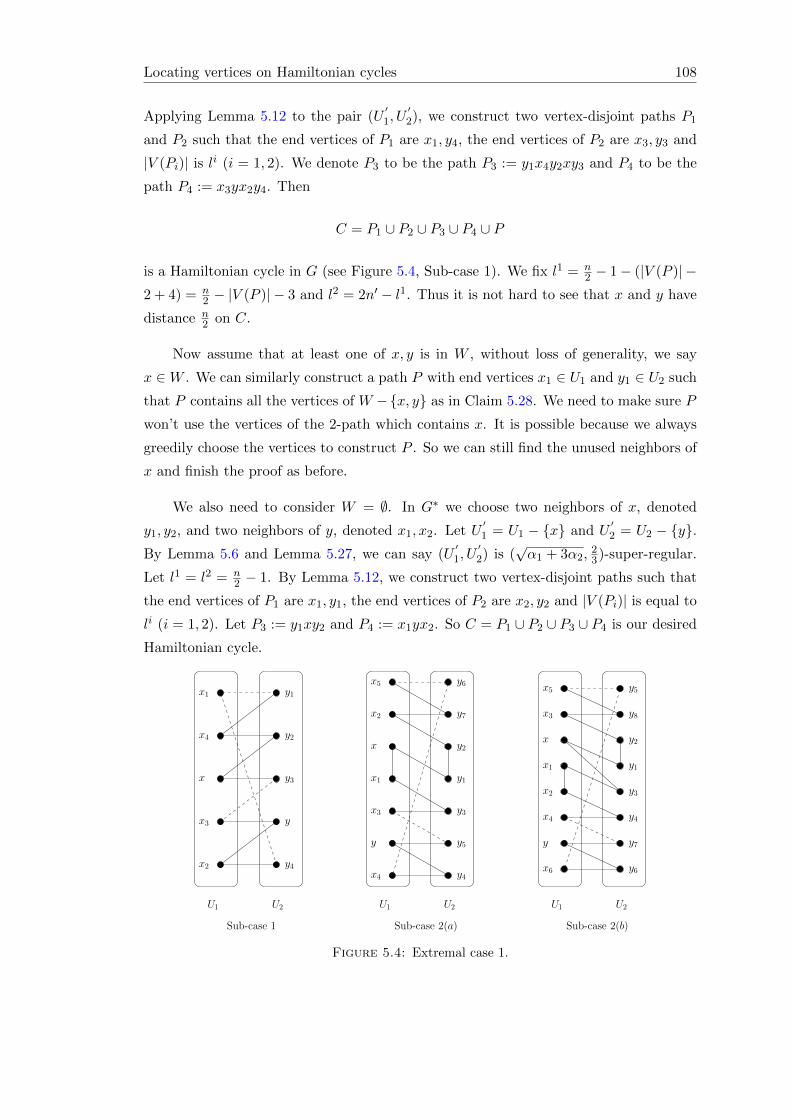
Locating vertices on Hamiltonian cycles 108
Applying Lemma 5.12 to the pair (U′1, U
′2), we construct two vertex-disjoint paths P1
and P2 such that the end vertices of P1 are x1, y4, the end vertices of P2 are x3, y3 and
|V (Pi)| is li (i = 1, 2). We denote P3 to be the path P3 := y1x4y2xy3 and P4 to be the
path P4 := x3yx2y4. Then
C = P1 ∪ P2 ∪ P3 ∪ P4 ∪ P
is a Hamiltonian cycle in G (see Figure 5.4, Sub-case 1). We fix l1 = n2 − 1− (|V (P )| −
2 + 4) = n2 − |V (P )| − 3 and l2 = 2n′ − l1. Thus it is not hard to see that x and y have
distance n2 on C.
Now assume that at least one of x, y is in W , without loss of generality, we say
x ∈W . We can similarly construct a path P with end vertices x1 ∈ U1 and y1 ∈ U2 such
that P contains all the vertices of W −x, y as in Claim 5.28. We need to make sure P
won’t use the vertices of the 2-path which contains x. It is possible because we always
greedily choose the vertices to construct P . So we can still find the unused neighbors of
x and finish the proof as before.
We also need to consider W = ∅. In G∗ we choose two neighbors of x, denoted
y1, y2, and two neighbors of y, denoted x1, x2. Let U′1 = U1 − x and U
′2 = U2 − y.
By Lemma 5.6 and Lemma 5.27, we can say (U′1, U
′2) is (
√α1 + 3α2,
23)-super-regular.
Let l1 = l2 = n2 − 1. By Lemma 5.12, we construct two vertex-disjoint paths such that
the end vertices of P1 are x1, y1, the end vertices of P2 are x2, y2 and |V (Pi)| is equal to
li (i = 1, 2). Let P3 := y1xy2 and P4 := x1yx2. So C = P1 ∪ P2 ∪ P3 ∪ P4 is our desired
Hamiltonian cycle.
U1 U2
x1
x3
x2
x4
x
y2
y
y1
y3
y4
y7
y1
x5 y6
x2
x
x1
y2
x3 y3
y y5
x4 y4
U1 U2
Sub-case 1 Sub-case 2(a)
x1
y7
x5
x3
x
x2
x4
y
x6
y5
y8
y2
y1
y3
y4
y6
U1 U2
Sub-case 2(b)
Figure 5.4: Extremal case 1.

Locating vertices on Hamiltonian cycles 109
Sub-case 2: suppose x, y are in the same part of G∗, without loss of generality, say
x, y ∈ U1.
Since the construction in Sub-case 1 is always in the bipartite graph (U1, U2) andn2 is odd, it seems that the same method doesn’t work in this case. Actually we need
some edges in G[U1] and G[U2] to change the parity.
Assume W 6= ∅ and x, y 6∈ W (if one of x, y is in W , the discussion is almost the
same as discussed before). Since δ(G) ≥ n2 + 1, x should have a neighbor in U1.
Assume this neighbor, denoted x1, is not y. We choose a neighbor of x in U2 −W ,
denoted y1, and choose a neighbor of y1 in U2, denoted y2. Whether x1 is in W or not,
we can find an unused neighbor of x1 in U2 −W , denoted y3, and choose an unused
neighbor of y3 in U1 − W , denoted x3. Whether y2 is in W or not, we can find an
unused neighbor of y2 in U1 −W , denoted x2. We choose two unused neighbors of y in
U2 −W , denoted y4, y5, and an unused neighbor of y4 in U1 −W , denoted x4. Since
degG∗(v) ≥ (1 − α1 − 2α2)n2 for all v 6∈ W , it is possible to choose all these vertices as
discussed in Sub-case 1. By the same method of Claim 5.28, we can construct a path P
with end vertices x5 ∈ U1 and y6 ∈ U2 such that P contains all the unused vertices of
W and |V (P )| ≤ 4|W |. Since the vertices used in P are greedily chosen, we can assume
that P won’t use any existing chosen vertices. We choose a common unused neighbor
of x2, x5 in U2 −W , denoted y7. Let
U′1 = U1 − V (P )− x, y, x1, x2, U
′2 = (U2 − V (P )− y1, y2, y3, y4, y7) ∪ y6.
Note that |U ′1| = |U ′2|, let |U ′1| = |U ′2| = n′. By Lemma 5.6 and n is sufficiently large,
(U′1, U
′2) is a (
√α1 + 11α2,
23)-super-regular pair. Applying Lemma 5.12 to the pair
(U′1, U
′2), we can construct two paths P1 and P2 such that the end vertices of P1 are x4, y6,
the end vertices of P2 are x3, y5 and |V (Pi)| = li (i = 1, 2). Let P3 := x5y7x2y2y1xx1y3x3
and P4 := x4y4yy5. Then
C = P1 ∪ P2 ∪ P3 ∪ P4 ∪ P
is a Hamiltonian cycle in G (see Figure 5.4, Sub-case 2(a)). We fix l1 = n2 −1−(|V (P )|+
5−1) = n2 −|V (P )|−5 and l2 = 2n′− l1. It is not hard to see that x and y have distance
n2 on C. Here we omit all the calculations about α, because it is almost same as Sub-case
1.
Now assume that y is the only neighbor of x in U1 but y has a neighbor which is
not x in U1, then the proof is similar to the proof in the last paragraph if we deal with
y first. We assume that y is the only neighbor of x in U1 and x is the only neighbor of
y in U1. We choose a neighbor of x in U2 −W , denoted y1. Since degG(y1) ≥ n2 + 1, y1
has a neighbor in U2, denoted y2. We choose another unused neighbor of x in U2 −W ,
Locating vertices on Hamiltonian cycles 110
denoted y3, and a neighbor of y3 in U1−W , denoted x1. Since degG(x1) ≥ n2 + 1, x1 has
a neighbor in U1, denoted x2. By our assumption, x2 should not be either of x and y.
We choose an unused neighbor of y2 in U1−W , denoted x3, an unused neighbor of x2 in
U2−W , denoted y4, and an unused neighbor of y4 in U1−W , denoted x4. By the same
method of Claim 5.28, we construct a path P with end vertices x5 ∈ U1 and y5 ∈ U2 such
that P contains all the unused vertices of W and |V (P )| ≤ 4|W |. We choose two unused
neighbors of y in U2 − V (P ), denoted y6, y7, and choose a neighbor of y6 in U1 − V (P ),
denoted x6, and choose a common unused neighbor of x3, x5 in U2 − V (P ), denoted y8.
Let
U′1 = U1 − V (P )− x, y, x1, x2, x3, U
′2 = (U2 − V (P )− y1, y2, y3, y4, y6, y8) ∪ y5.
Note that |U ′1| = |U ′2|, let |U ′1| = |U ′2| = n′. By Lemma 5.6 and n is sufficiently
large, (U′1, U
′2) is a (
√α1 + 11α2,
23)-super-regular pair. Applying Lemma 5.12 to the
pair (U′1, U
′2), we can construct two paths P1 and P2 such that the end vertices of
P1 are x6, y5, the end vertices of P2 are x4, y7 and |V (Pi)| = li (i = 1, 2). Let
P3 := x5y8x3y2y1xy3x1x2y4x4 and P4 := x6y6yy7. Then
C = P1 ∪ P2 ∪ P3 ∪ P4 ∪ P
is a Hamiltonian cycle in G (see Figure 5.4, Sub-case 2(b)). Let l1 = n2 −|V (P )|− 5 and
l2 = 2n′ − l1. Thus x and y have distance n2 on C. We can say all the choices of the
vertices are possible because of the minimum degree of G∗. We omit all these similar
calculations here.
If W is empty, we take the path P be an edge. The rest of the proof is the same as
above.
At the end we need to consider the case when n2 is even. Actually if x, y are in the
same part of G∗, the proof is similar to Sub-case 1, and if x, y are in different parts of
G∗, the proof is similar to Sub-case 2.
5.4.2 Extremal case 2
Suppose G is a graph on n vertices with δ(G) ≥ n2 + 1 and there exists a balanced
partition of V (G) into V1 and V2 such that the density d(V1, V2) ≤ α. We suppose
α ≤ (19)3. Let α1 = α
13 and α2 = α
23 .
We also need a similar lemma as Lemma 5.27.
Lemma 5.29. If G is in extremal case 2, then V (G) can be partitioned into two balanced
parts U1 and U2 such that

Locating vertices on Hamiltonian cycles 111
(a) there is a set W1 ⊆ U1 (respectively W2 ⊆ U2 ) such that there exist vertex-
disjoint 2-paths in G[U1] (respectively G[U2] ) with the vertices of W1 (respectively W2 )
as the internal vertices in each 2-path and |W1| ≤ α2n2 (respectively |W2| ≤ α2
n2 ) ;
(b) degG[U1](u) ≥ (1− α1 − 2α2)n2 for all u ∈ U1 −W1 and degG[U2](v) ≥ (1− α1 −2α2)n2 for all v ∈ U2 −W2.
Proof. The argument is similar to the proof of Lemma 5.27. For some similar claims,
we just give them without proofs.
For i = 1, 2, let V ∗i = v ∈ Vi : deg(v, Vi) ≥ (1 − α1)n2 . We can claim that
|Vi − V ∗i | ≤ α2n2 since otherwise d(V1, V2) >
α1n2·α2
n2
n2·n2
= α, a contradiction.
For any vertex v ∈ Vi − V ∗i , if deg(v, V3−i) ≥ (1− α1)n2 , we also add it to V ∗3−i. We
denote the final two sets by V′i (i = 1, 2) and let V0 = V − V ′1 − V
′2 . Thus |V0| ≤ α2n.
For every vertex v in V′i , deg(v, V
′i ) ≥ (1− α1)n2 − α2
n2 (i = 1, 2). For every vertex u in
V0, deg(u, V′i ) ≥ (n2 − (1− α1)n2 )− α2
n2 ≥ (α1 − α2)n2 (i = 1, 2).
First, we assume |V ′1 |, |V′
2 | ≤ n2 . Then we add all the vertices in V0 to V
′1 and V
′2
such that the final two sets are of the same size. Denote the final two sets by U1 and
U2. Let W1 = U1 − V′
1 and W2 = U2 − V′
2 , then V0 = W1 ∪W2. Since for each vertex
u ∈W1, deg(u, V′
1 ) ≥ (α1 − α2)n2 ≥ 2α2n ≥ 2|V0|, we can greedily choose two neighbors
of u in V′
1 such that the neighbors of all the vertices in W1 are distinct. So W1 and U1
are what we need. It is same to find 2-paths in G[U2]. The degree conclusion also holds.
Second, without loss of generality we assume |V ′1 | > n2 . Let V 0
1 be the set of vertices
v ∈ V ′1 such that deg(v, V′
2 ) ≥ α1n2 .
If |V 01 | ≥ |V
′1 |− n
2 , we take W2 to be the set of all vertices of V0 and |V ′1 |− n2 vertices
of V 01 and W1 to be an empty set. Let U1 = V
′1 −W2 and U2 = V
′2 ∪W2. So |W2| ≤ α2
n2 .
For every vertex u ∈ W2, we have deg(u, V′
2 ) ≥ (α1 − α2)n2 − α2n2 ≥ α2n ≥ 2|W2|.
Thus we can greedily choose two neighbors of u in V′
2 such that the neighbors of all the
vertices in W2 are distinct. U1, U2, W1, W2 are what we need.
Now we assume |V 01 | < |V
′1 | − n
2 . Let U1 = V′
1 − V 01 and U2 = V
′2 ∪ V0 ∪ V 0
1 . Let
t = |U1| − n2 , so t ≤ α2
n2 . We consider the bipartite graph (U1, V
′2 ). Suppose that
(U1, V′
2 ) has a biggest family of vertex-disjoint 2-paths on a vertex set S, such that the
internal vertices of these 2-paths are in U1 and the end vertices of these 2-paths are in
V′
2 . Let S = S1∪S2 with the internal vertex set S1 ⊆ U1 and the end vertex set S2 ⊆ V′
2 .
Suppose |S1| = s, |S2| = 2s. We use δ∗ to denote the minimum degree of vertices of V′
2
in (U1, V′
2 ). So δ∗ ≥ n2 + 1 − (n2 − t − 1) = t + 2. We use ∆∗ to denote the maximum

Locating vertices on Hamiltonian cycles 112
degree of vertices of U1 in (U1, V′
2 ). So ∆∗ < α1n2 . Then
δ∗(|V ′2 | − 2s) ≤ e(V ′2 − S2, U1) ≤ s(∆∗ − 2) + (n
2+ t− s).
By some calculations, we can get
s ≥(t+ 2)|V ′2 | − (n2 + t)
∆∗ + 2t+ 1
≥(t+ 2)(1− α2)n2 −
n2 − α2
n2
α1n2 + 1 + 2α2
n2
=(t+ 1)(1− α2)n2 − 2α2
n2
(α1 + 2α2)n2 + 1
Since n can be sufficiently large, we can conclude s > t.
We pick t vertex-disjoint 2-paths with the internal vertex set S1 ⊆ U1 and move the
vertices of S1 into U2. Now we get |U1| = |U2| = n2 . Let W2 = V0 ∪ V 0
1 ∪ S1 and W1 be
an empty set. For every vertex u ∈ V0 ∪ V 01 , degG[U2](u) ≥ (α1 − α2)n2 − α2
n2 ≥ 2|W2|.
We can greedily find disjoint 2-paths in G[V0∪V 01 , V
′2 ] with all the vertices of V0∪V 0
1 as
internal vertices such that these 2-paths are all disjoint with the existing 2-paths. U1,
U2, W1, W2 are what we need.
For a graph G in extremal case 2, we apply Lemma 5.29 to G and get a partition
of V (G) = U1 ∪ U2 with the properties in Lemma 5.29.
First, assume x and y are in different parts in the partition of V (G), without loss
of generality, we say that x ∈ U1 and y ∈ U2. Since δ(G) ≥ n2 + 1, x (respectively y)
should have at least two neighbors in U2 (respectively U1). Denote a neighbor of x in U2
by x1 and a neighbor of y in U1 by y1 such that x1 6= y and y1 6= x. Since the 2-paths
are all greedily chosen in Lemma 5.29, we can assume that x, y, x1, y1 are not the end
vertices of those 2-paths.
Claim 5.30. There is a Hamiltonian path in G[U1] with end vertices x and y1.
Proof. Whether x and y1 are inW1 or not, we can find a neighbor of x in U1−W1, denoted
u, and a neighbor of y1 in U1 −W1, denoted v. Suppose W1 − x, y1 = w1, w2, ..., wtand the two end vertices of the 2-path containing wi are ai, bi. Since degG[U1](ai) ≥(1 − α1 − 2α2)n2 and degG[U1](bi) ≥ (1 − α1 − 2α2)n2 , we can greedily choose ci ∈ U1
which is a common neighbor of ai+1 and bi (1 ≤ i ≤ t − 1). Moreover we can choose
all these ci to be distinct. We also greedily choose ct which is a common neighbor
of bt and v. Then P1 = a1w1b1c1a2w2b2c2...bt−1ct−1atwtbtctv is a path containing all

Locating vertices on Hamiltonian cycles 113
the vertices of those 2-paths (except the 2-paths containing x, y1, if x, y1 are in W1).
|V (P1)| = 4t+ 1 ≤ 4α2n2 + 1.
Let U∗ = (U1 − V (P )− x, y1) ∪ a1. We consider the induced subgraph G[U∗].
For any vertex w ∈ U∗, degG[U∗](w) ≥ (1−α1−2α2)n2 −4α2n2 −2. Since n is sufficiently
large and α ≤ (19)3, degG[U∗](w) ≥ (1 − α1 − 7α2)n2 > n
4 + 1 ≥ |U∗|2 + 1 for any vertex
w ∈ U∗. So G[U∗] is Hamiltonian-connected. We can find a path P2 in G[U∗] with end
vertices u, a1 containing all the vertices of U∗. Then H1 = xu ∪ P1 ∪ P2 ∪ vy1 is a
Hamiltonian path in G[U1] with end vertices x and y1.
By the same method, we can construct a Hamiltonian path H2 in G[U2] with end
vertices y and x1. So
C = xx1, yy1 ∪H1 ∪H2
is a Hamiltonian cycle in G such that distC(x, y) = n2 (see Figure 5.5 (a)).
U1 U2
x y2
y3
y y5
U1 U2
x
y
U1 U2
(c)(a) (b)
x x1
yy1
x1
v u
y1
yv1
v3
v2
u1
Figure 5.5: Extremal case 2.
Now assume x and y are in the same part in the partition of V (G), without loss of
generality, say x, y ∈ U1. Since δ(G) ≥ n2 +1, x and y should have at least two neighbors
in U2. We choose a neighbor of x in U2, denoted x1, and a neighbor of y in U2, denoted
y1, such that x1 6= y1. Since the 2-paths are all greedily chosen in Lemma 5.29, we can
assume that x, y, x1, y1 are not the end vertices of those 2-paths.
Assume there is a vertex u ∈ U2 − x1, y1 such that it has two neighbors u1, u2 ∈U1−x, y. We also assume that u1, u2 are not the end vertices of the 2-paths. Whether
x, u2 are in W1 or not, we claim that we can find a path of length at most four with
end vertices x and u2 in G[U1]. Indeed, the worst case is when x, u2 are both in W1.
We can find a neighbor of x in U1 −W1, denoted v1, and a neighbor of u2 in U1 −W1,
denoted v2. We choose a common neighbor of v1, v2 in G[U1], denoted v3. xv1v3v2u2 is
a path of length four with end vertices x and u2 in G[U1]. Then we can construct a path
with end vertices x1 and u1, denote it by P1 = x1xv1v3v2u2uu1. By the same method

Locating vertices on Hamiltonian cycles 114
in the proof of Claim 5.30, we construct a path P2 in G[U1] with end vertices u1 and y,
containing all the vertices of U1 − V (P1). In G[U2], by the same method in the proof of
Claim 5.30, we can construct a path P3 with end vertices x1 and y1, containing all the
vertices of U2 − u. So
C = P1 ∪ P2 ∪ P3 ∪ yy1
is a Hamiltonian cycle in G such that distC(x, y) = n2 (see Figure 5.5 (b)).
Assume there is a vertex u ∈ U2 − x1, y1 such that only one of the neighbors of
u in U1 is equal to x or y, without loss of generality, we assume that u1, u2, the two
neighbors of u, satisfy that u2 = x but u1 6= y. Let P1 = x1xuu1. The rest construction
is the same as in the last paragraph.
At last we assume that in U1, the neighbors of all the vertices of U2 − x1, y1 are
x and y. That means any vertex in U1 − x, y is adjacent to x1 and y1. We choose a
neighbor of x in U2, denoted u, and a neighbor of x1 in U1, denoted v. We construct a
path P1 = vx1xu. By the same method in the proof of Claim 5.30, we can construct a
path P2 in G[U1] with end vertices v and y, containing all the vertices of U1 − x, and
a path P3 in G[U2] with end vertices u and y1, containing all the vertices of U2 − x1.So
C = P1 ∪ P2 ∪ P3 ∪ yy1
is a Hamiltonian cycle in G such that distC(x, y) = n2 (see Figure 5.5 (c)).
5.5 Concluding remarks and further work
In this chapter, we gave a proof of Enomoto’s conjecture for graphs of sufficiently large
order. Actually, our approach also works for proving Conjecture 1.51, we will show this
in the next chapter.
Note that, our proof is for graphs of sufficiently large order, but how large is it?
That is the common question when we use Regularity Lemma. We try to prove the
Theorem 5.2 without using Regularity Lemma, but unfortunately, we did not succeed
yet. Recently, there are some works on how the use of the Regularity Lemma and
the Blow-up Lemma can be avoided in certain extremal problems of dense graphs (see
[65]). This gives us positive sign to find a way to prove Theorem 5.2 avoiding using the
Regularity Lemma in future.

Chapter 6
Distributing pairs of vertices on
Hamiltonian cycles
In this chapter we give a proof of Conjecture 1.51 for graphs of sufficiently large order.
It is kind of continue work of Chapter 5. To make it easier to read, we state again
Conjecture 1.51 here.
Conjecture 6.1. [33] If G is a graph of order n ≥ 3 and δ(G) ≥ n2 + 1, then for any
pair of vertices x, y in G and any integer 2 ≤ k ≤ n2 , there is a Hamiltonian cycle C of
G such that distC(x, y) = k.
Our main result is the Theorem 1.53. We state again this theorem here.
Theorem 6.2. [47] There exists a positive integer n0 such that for all n ≥ n0, if G is
a graph of order n with δ(G) ≥ n2 + 1, then for any pair of vertices x, y in G and any
integer 2 ≤ k ≤ n2 , there is a Hamiltonian cycle C of G such that distC(x, y) = k.
6.1 Introduction
In Chapter 5, we gave a proof of Enomoto’s conjecture for graphs of sufficiently large
order.
Theorem 6.3 (Theorem 5.2). There exists a positive integer n0 such that for all n ≥ n0,
if G is a graph of order n with δ(G) ≥ n2 + 1, then for any pair of vertices x, y in G,
there is a Hamiltonian cycle C of G such that distC(x, y) = bn2 c.
Here we will prove that Faudree-Li conjecture is true for graphs of sufficiently large
order by showing Theorem 6.2.
115
Distributing vertices on Hamiltonian cycles 116
The main idea and the main tools of the proof of Theorem 6.2 and Theorem 5.2 are
similar, but there are also some differences since in Theorem 5.2, any two given vertices
are required to be located on a Hamiltonian cycle of distance half of the order of the
graph, while in Theorem 6.2 the distance is extended from half of the order of the graph
to two. We don’t want to just point out the differences between the proofs of Theorem
6.2 and Theorem 5.2, to make this chapter complete, we will give the whole proof of
Theorem 6.2. We will follow all the notations, such as balanced partition, reduced graph
et al. as in Chapter 5.
6.2 Outline of the proof
In our proof for Theorem 6.2 we will use the Regularity Lemma-Blow-up Lemma method
as many other studies. Some claims and lemmas in our proof are similar as in Chapter
5. We will give these claims and lemmas without proofs here.
We first consider the graphs of even order n. We assume that n is sufficiently large
and fix the following sequence of parameters,
0 < ε d α 1. (6.1)
By Theorem 1.48 and Theorem 6.3, we assume that the required distance k satis-
fying
n
6< k <
n
2. (6.2)
We define two extremal cases as follows.
Extremal Case 1: There exists a balanced partition of V (G) into V1 and V2 such
that the density d(V1, V2) ≥ 1− α.
Extremal Case 2: There exists a balanced partition of V (G) into V1 and V2 such
that the density d(V1, V2) ≤ α.
We will prove Theorem 6.2 for the non-extremal case in Section 6.3 and for the
extremal cases in Section 6.4. The proof will include some sub-cases discussions because
of the parity of k.
When n is odd, we pick a vertex z 6= x or y of the graph G and consider the
induced graph G[V (G)−z]. Since the order of the graph G[V (G)−z] is even, we use the
similar proof as above in G[V (G)− z] and obtain a Hamiltonian cycle in G[V (G)− z].
Distributing vertices on Hamiltonian cycles 117
Then we “insert” z into this cycle and make sure x, y have distance k on the resulting
Hamiltonian cycle of G. In Section 6.3 and 6.4, the proof will include all the discussions
when n is odd.
6.3 Non-extremal case
6.3.1 The graph order n is even
Step 1. Applying the Regularity Lemma.
Let G be a graph of even order which is not either of the extremal cases. We apply
the Regularity Lemma to G with parameters ε, d,m0 to obtain a partition of G into
clusters V1,...,Vl and an exception set V0, and a spanning subgraph G′. Assume that l
is even, if not, we move the vertices of one of the clusters into V0 to make l be an even
number. Now |V0| ≤ 2εn and lL ≥ (1− 2ε)n. Let s := l2 .
Let R be the reduced graph of G.
The following claim, which is proved in Chapter 5, shows that R inherits the mini-
mum degree condition.
Claim 6.4. δ(R) ≥ (12 − 2d)l.
As shown in Chapter 5, R is Hamiltonian.
Let CR be a Hamiltonian cycle in R. We choose two distinct clusters X, Y which
are as close as possible on CR such that x is friendly to Y and y is friendly to X. The
following claim is proved in Chapter 5.
Claim 6.5. We can choose distinct clusters X and Y such that x is friendly to Y , y is
friendly to X and distCR(X,Y ) ≤ 3dl.
By Claim 6.5 we choose these two clusters X and Y and give a new notation for
all clusters except V0 as follows. We choose a direction of CR, which is along the longer
path from Y to X on CR (there are two paths from Y to X on CR, and we choose the
longer one). Starting from Y , we denote the clusters by Y1, X2, Y2, X3, Y3,..., Xs, Ys,
X1 along this direction. Y is denoted by Y1 and X is denoted by a Xi or a Yi.
Step 2. Constructing paths to connect Yi and Xi+1 (with Xs+1 = X1) for 1 ≤ i ≤ s.
Distributing vertices on Hamiltonian cycles 118
In this step, the parity of k and the new notation of X will affect our constructions.
We first assume that k is even and X is denoted by Yt for some 1 < t ≤ s. We call Xi,
Yi partners of each other (1 ≤ i ≤ s).
By Claim 6.5, distCR(Y1, Yt) = l − 2t+ 2 ≤ 3dl. So
t− 1 ≥ 1− 3d
2l. (6.3)
Let wx, y11 ∈ Y1 be two neighbors of x such that wx is friendly to X2 and y1
1 is
friendly to X1. Since x is friendly to Y1, x has at least (d − ε)L neighbors in Y1. By
Lemma 5.3, at least (d − ε)L − εL vertices can be chosen as wx (also true for y11). Let
x12 ∈ X2 be a neighbor of wx such that x1
2 is friendly to Y2. By Lemma 5.3, at least
(d− ε)L− εL vertices can be chosen as x12. We obtain a path P1 = y1
1xwxx12 connecting
Y1 and X2. We call this procedure joining x to Y1 and x behaves like a vertex in X1.
Let y21 ∈ Y1 be a vertex friendly to X1 and let x2
2 ∈ X2 be a neighbor of y21 such that
x22 is friendly to Y2. By Lemma 5.3, this choice of y2
1 and x22 is possible and make them
be distinct with the vertices in P1. We obtain another path Q1 = y21x
22. Similarly we
can construct paths Pt = y1t ywyx
1t+1 and Qt = y2
t x2t+1, where y1
t , y2t ∈ Yt is friendly to
Xt, x1t+1, x
2t+1 ∈ Xt+1 is friendly to Yt+1 and wy ∈ Yt. We call this procedure joining y
to Yt and x behaves like a vertex in Xt. For 1 ≤ i ≤ s and i 6= 1, t, let y1i ∈ Yi (resp.
y2i ∈ Yi) be a vertex friendly to Xi and x1
i+1 ∈ Xi+1 (resp. x2i+1 ∈ Xi+1) be a neighbor
of y1i (resp. y2
i ) such that x1i+1 (resp. x2
i+1) is friendly to Yi+1. Here x11 = x1
s+1 and
x21 = x2
s+1. Let Pi = y1i x
1i+1 and Qi = y2
i x2i+1 (1 ≤ i ≤ s and i 6= 1, t). By Lemma 5.3,
we can make sure all these paths are vertex-disjoint.
In summary, we have constructed paths Pi and Qi, which are vertex-disjoint and
connect Yi and Xi+1 (1 ≤ i ≤ s), x is on P1 and y is on Pt. Each end vertex of these
paths is friendly to its cluster’s partner. We use INT to denote the vertex set of all
internal vertices on all Pi’s and Qi’s. Now INT = x, y, wx, wy.
For every 1 ≤ i ≤ s, let
X′i := u ∈ Xi : deg(u, Yi) ≥ (d− ε)L, Y ′i := v ∈ Yi : deg(v,Xi) ≥ (d− ε)L.
Since (Xi, Yi) is ε-regular, we have |X ′i |, |Y′i | ≥ (1 − ε)L. We move all the vertices
in Xi − X′i and Yi − Y
′i to V0. If |X ′i | 6= |Y
′i |, say |X ′i | > |Y
′i |, we choose an arbitrary
subset of X′i of size |Y ′i | and still name it X
′i . We still denote the set V0 ∪
⋃ki=1(Xi −
X′i) ∪
⋃ki=1(Yi − Y
′i ) by V0. We also remove all the vertices in INT out of V0, X
′i and
Y′i . This may cause that some (X
′i , Y
′i ) is not balanced. For example, if wx ∈ Y
′1 and
we remove it from Y′
1 , then (X′1, Y
′1 ) be not balanced. In this example, to make sure
(X′1, Y
′1 ) is balanced, we move one vertex in X
′i to V0. We do the same operations for all

Distributing vertices on Hamiltonian cycles 119
the vertices in INT . Since |INT | = 4 and n is sufficiently large, at most εLl + 4 ≤ 2εn
vertices are moved to V0. We derive that |V0| ≤ 4εn and |X ′i | = |Y ′i | ≥ (1 − ε)L − 1
(1 ≤ i ≤ s) in this step. Since εL ≥ ε (1−2ε)nl ≥ ε(1−2ε)
M0n and n is sufficiently large, we
say εL ≥ 1. Thus |X ′i | = |Y ′i | ≥ (1 − 2ε)L (1 ≤ i ≤ s). The minimum degree in each
pair is at least (d− ε)L− εL− 1 ≥ (d− 3ε)L. We also can say (X′i , Y
′i ) is 2ε-regular by
Slicing Lemma.
Now assume that k is even and X is denoted by Xt for some 1 ≤ t ≤ s. We
construct P2 = y12x
13 and Q2 = y2
2x23 as before. Since δ(G) ≥ n
2 + 1, any two vertices
have at least two common neighbors. Suppose that y12, x
13 have a common neighbor u1
and y22, x
23 have a common neighbor u2 6= u1. First, if u1 and u2 are both different with
x and y, then we choose P2 = y12u1x
13 and Q2 = y2
2u2x23. We join x to Y1, join y to
Xt and continue all the other constructions of Pi’s and Qi’s as before. In this case x
is on P1 and y is on Pt−1. Second, assume that we cannot find these required vertices
y12, x
13, y
22, x
23 such that u1 and u2 are both different with x and y. We choose y1
2, y22 to
be friendly to X2 and X3. There are at least (1− 2ε)L possible choices for y12 and it is
similar for y22. We choose x1
3 to be a neighbor of y12 and friendly to Y2 and Y3. There
are at least (d − ε)L − 2εL = (d − 3ε)L possible choices for x13 and it is similar for x2
3.
By the assumption every these possible y12, x
13, y
22, x
23 should be neighbors of x or y. So
x or y should have at least 12(d− 3ε)L neighbors in Y2 and also in X3. If y has at least
12(d − 3ε)L neighbors in in Y2 and in X3, we change the choice of X and choose Y2 to
be the X. Here X = Y2 and Y = Y1, so distCR(X,Y ) = 2. Otherwise, x has at least
12(d− 3ε)L neighbors in Y2 and in X3. We change the choice of Y and choose X3 to be
the Y . In this case X = Xt and Y = X3, so distCR(X,Y ) ≤ 3dl + 3 by Claim 6.5. We
give a new notation for all clusters except V0 according to the new choice of X,Y and
construct Pi’s, Qi’s as before. In this new notation, we still say we join x to Y1 and join
y to Yt for a new t. We need to mention that (6.3) may have slight difference as follows,
but it won’t affect the calculation in the following Claim 6.7.
We also need to consider the case when k is odd. Actually if k is odd and X is
denoted by Xt′ for some 1 ≤ t′ ≤ s, the discussions in this case is similar as in the case
when k is even and X is denoted by Yt for some 1 ≤ t ≤ s. And if k is odd and X is
denoted by Yt′ for some 1 ≤ t′ ≤ s, the discussions in this case is similar as in the case
when k is even and X is denoted by Xt for some 1 ≤ t ≤ s. We omit all these similar
arguments here.
Step 3. Extending Qi’s (1 ≤ i ≤ s) by using all the vertices of V0.
If a vertex v is friendly to a cluster X, we denote this relation by v ∼ X. If two
clusters X and Y are a regular pair, we denote this relation by X ∼ Y . Given two

Distributing vertices on Hamiltonian cycles 120
vertices u, v ∈ V (G), a u, v-chain of length 2s with distinct clusters A1, B1, ..., As, Bs is
u ∼ A1 ∼ B1 ∼ · · · ∼ As ∼ Bs ∼ v and Aj , Bj = Xi, Yi for some 1 ≤ i ≤ k. We can
say that for each pair of vertices in V0 we have the following claim, which is proved in
Chapter 5.
Claim 6.6. For each pair of vertices u, v in V0, we can find u, v-chains of length at
most four such that every cluster is used in at most d10L chains.
Now we extend Qi’s (1 ≤ i ≤ s). By Claim 6.6, we construct chains of length at
most four for each pair such that every cluster is used in at most d10L chains. We deal
with the vertices of V0 pair by pair. Assume that we deal with the pair (u, v) now.
Denote X∗i = X′i − INT and Y ∗i = Y
′i − INT .
We first consider the case when the u, v-chain has length two. Without loss of
generality, assume that this chain is u ∼ Xi ∼ Yi ∼ v, for some 1 ≤ i ≤ s. Let w1 ∈ Y ∗ibe a neighbor of x2
i and let w2 ∈ X∗i be a neighbor of u such that w1 and w2 are
adjacent. By Slicing Lemma, we can say this choice is possible. Let w3 ∈ X∗i be another
neighbor of u. To include u, we extend Qi−1 to Qi−1 ∪x2iw1, w1w2, w2u, uw3. We still
denote this new path by Qi−1 and denote the end vertex w3 of this path by the new x2i .
Since u behaves like a vertex in Yi on Qi−1, we call this procedure inserting u into Yi
by extending Qi−1. Similarly, let w4 ∈ X∗i be a neighbor of y2i and let w5, w6 ∈ Y ∗i be
two neighbors of v such that w4 and w5 are adjacent. To include v, we extend Qi to
Qi ∪ y2iw4, w4w5, w5v, vw6. We still denote this new path by Qi and denote the end
vertex w6 of this path by the new y2i . Since v behaves like a vertex in Xi on Qi, we
call this procedure inserting v into Xi by extending Qi. And we update the set INT .
Indeed, three vertices of X∗i are added to INT (also for Y ∗i ) and totally eight vertices
are added to INT including u, v.
Now we consider that the u, v-chain has length four. Without loss of generality,
we assume that the chain is u ∼ Xi ∼ Yi ∼ Xj ∼ Yj ∼ v, for some i, j. We extend
the path Qi−1 by inserting u into Yi. We choose a vertex of Y ∗i which is friendly to Xj
and insert it into Yj to extend Qj−1. At last we extend the path Qj by inserting v into
Xj . Meanwhile, we update the set INT . Indeed, two vertices of X∗i are added to INT
(also for Y ∗i ) and three vertices of X∗j are added to INT (also for Y ∗j ). So totally twelve
vertices are added into INT including u, v.
In each time inserting the vertex pair (u, v), the cluster pair (X∗i , Y∗i ) is still balanced
and at most three vertices of a cluster in the chain are used. So
|X∗i | = |Y ∗i | ≥ (1− 2ε)L− 3d
10L ≥ (1− d
2)L
provided ε < d10 .

Distributing vertices on Hamiltonian cycles 121
For each vertex u ∈ X∗i , we have
deg(u, Y ∗i ) ≥ (d− 3ε)L− 3d
10L ≥ d
2L
provided ε < d15 . And it is the same for the degree of any vertex in Y ∗i .
By Slicing Lemma, we can say the pair (X∗i , Y∗i ) is (2ε, d2)-super-regular (1 ≤ i ≤ s).
We continue this process till there is no vertices left in V0.
Step 4. Constructing the desired Hamiltonian cycle.
In this step, we use Lemma 5.12 to construct two paths W 1i and W 2
i in each pair
(X∗i , Y∗i ) (1 ≤ i ≤ s). Then we combine all these paths with Pi’s and Qi’s to obtain
a Hamiltonian cycle in G. At last we adjust the length of W 1i and W 2
i in each pair to
make sure that x and y have distance k on this Hamiltonian cycle.
For each 1 ≤ i ≤ s, we choose any even integers l1i , l2i such that 4 ≤ l1i , l2i ≤ 2|X∗i |−4
and l1i + l2i = 2|X∗i |. We will adjust these integers later.
For 2 ≤ i ≤ s, by Lemma 5.12, we construct two paths W 1i and W 2
i in the pair
(X∗i , Y∗i ) such that
(a) W 1i has end vertices x1
i and y1i with |V (W 1
i )| = l1i ;
(b) W 2i has end vertices x2
i and y2i with |V (W 2
i )| = l2i .
And for i = 1, we construct two paths W 11 and W 2
1 in the pair (X∗1 , Y∗
1 ) such that
(c) W 11 has end vertices x1
1 and y12 with |V (W 1
1 )| = l11;
(d) W 21 has end vertices x2
1 and y21 with |V (W 1
2 )| = l12.
It is not hard to see
C = P1 ∪ (k⋃i=2
(W 1i ∪ Pi)) ∪W 1
1 ∪Q1 ∪ (k⋃i=2
(W 2i ∪Qi)) ∪W 2
1
is a Hamiltonian cycle in G (See Figure 6.1).
Now we adjust the values of l1i and l2i (1 ≤ i ≤ s) to make sure that x and y have
distance k on the Hamiltonian cycle.
Claim 6.7. We can properly choose the value of l1i (2 ≤ i ≤ s) such that distC(x, y) = k.
Proof. Without loss of generality, we consider the case when k is even and X is denoted
by Yt in the beginning of the second step. Since x is on P1 and y is on Pt, we consider

Distributing vertices on Hamiltonian cycles 122
Y ∗1X∗1 X∗2 Y ∗2 X∗3 Y ∗3
Pk P1 P2 P3
Qk Q1 Q2 Q3
Figure 6.1: Construction of the Hamiltonian cycle
the path P := P1 ∪ (⋃ti=2(W 1
i ∪Pi)) to make sure x and y have distance k on this path.
That means the number of vertices between x and y on P should be k − 1. Among the
vertices between x and y on P , the only vertex not belong to W 1i (2 ≤ i ≤ t) is wx.
Thus we need to make sure
k − 1 =
t∑i=2
l1i + 1. (6.4)
Since k is even and all these l1i ’s are also even, there is no parity problem. We say
thatt∑i=2
l1i can be any even value satisfying
n
6− 2 <
t∑i=2
l1i <n
2− 2. (6.5)
Since by Lemma 5.12, l1i can be any even integer such that 4 ≤ l1i ≤ 2|X∗i | − 4.
By |X∗i | ≥ (1− d2)L, we can choose l1i such that
t∑i=2
l1i can be any even integer with the
following bound,
4(t− 1) ≤t∑i=2
l1i ≤ 2(t− 1)(1− d
2)L− 4(t− 1) = 2(t− 1)((1− d
2)L− 2).
We know that t ≤ s = l2 , then 4(t−1) < 2l. Since l ≤M0 in the Regularity Lemma
and n is sufficiently large (let n ≥ 12(M0 + 1)), we can say that 4(t− 1) < 2l ≤ 2M0 ≤n6 − 2.
By (6.3), we also know t− 1 ≥ 1−3d2 l, so
2(t− 1)((1− d
2)L− 2) ≥ (1− 3d)(1− d
2)lL− 2(1− 3d)l
≥ (1− 7
2d)(1− 2ε)n− 2l
≥ (1− 4d)n− 2M0 ≥3
4n− 2M0,

Distributing vertices on Hamiltonian cycles 123
provided 4ε ≤ d ≤ 116 and l ≤ M0. Since n is sufficiently large (let n ≥ 8M0), we can
say that 2(t− 1)((1− d2)L− 2) ≥ 3
4n− 2M0 ≥ n2 .
Thus we have proved thatt∑i=2
l1i can be any even value satisfying (6.5). By our
assumption (6.2), n6 < k < n
2 . So it is possible to choose l1i (2 ≤ i ≤ t) such thatt∑i=2
l1i
satisfying (6.4).
We choose l1i (2 ≤ i ≤ t) such that (6.4) holds and arbitrarily choose the even
integers l11, l1i (t < i ≤ k) with the conditions in Lemma 5.12. Thus distC(x, y) = k.
6.3.2 The graph order n is odd
We pick a vertex z 6= x or y and assume that G[V −z] is a graph which is not either of the
extremal cases. The order of the induced graphG[V−z] is n−1 and δ(G[V−z]) ≥ n−12 +1.
We apply the proof above to G[V − z] and obtain a Hamiltonian cycle C in G[V − z]such that distC(x, y) = k. We denote the longer path between x and y on C by P (x, y),
i.e. the distance of x and y on P (x, y) is n− 1− k. Since δ(G) ≥ n2 + 1, z has at least
two neighbors such that they are adjacent on C.
If there exist two vertices u, v ∈ P (x, y) such that they are neighbors of z and
adjacent in P (x, y), then replacing the edge uv in C by the path uzv we can obtain a
Hamiltonian cycle C∗ in G such that distC∗(x, y) = k.
Otherwise, this kind of two vertices u, v are on the shorter path between x and y
on C. We make the shorter path between x, y on C be the longer one by adjusting the
values of l1i ’s. Precisely, we consider the path P = P1 ∪ (⋃ti=2(W 1
i ∪Pi)) as in Claim 6.7
and make sure distP (x, y) = n− 1− k.
If uv ∈ E(Pi) for some 1 ≤ i ≤ t, we need to make sure that
n− k − 2 =
t∑i=2
l1i + 1. (6.6)
Since n is sufficiently large, we can say 4(t−1) ≤ n2−2 and 2(t−1)((1− d
2)L−2) ≥ 56n−2
similarly as in Claim 6.7. Sot∑i=2
l1i can be any even value satisfying n2−2 <
t∑i=2
l1i <56n−2.
Since n6 < k < n
2 , we can choose the value of l1i (2 ≤ i ≤ t) satisfying (6.6). By Lemma
5.12, we construct new paths in the pairs of clusters according to the new choice of l1i ’s
and obtain a new Hamiltonian cycle C′
in G[V − z]. Now the edge uv is in the longer
path between x and y on C′. Replacing uv by uzv in C
′, we get our desired Hamiltonian
cycle in G.

Distributing vertices on Hamiltonian cycles 124
Now assume that uv ∈ E(W 1i ) for some 2 ≤ i ≤ t, without loss of generality, we say
uv ∈ E(W 12 ). We fix the values of l12, l22 and the paths W 1
2 , W 22 , and adjust the values
of l1i ’s (3 ≤ i ≤ t) to make sure distP (x, y) = n − 1 − k. By some similar calculations
as above, we can choose the values of l1i ’s (3 ≤ i ≤ t) satisfying (6.6). Then by the new
constructions of paths in the pairs (X∗i , Y∗i ) according to the new choice of l1i (3 ≤ i ≤ t),
we can get a new Hamiltonian cycle C′′
in G[V −z] such that the edge uv is in the longer
path between x and y on C′′. Replacing uv by uzv in C
′′, we get a new Hamiltonian
cycle of G such that the distance between x and y on this cycle is k.
6.4 Extremal cases
6.4.1 Extremal case 1
6.4.1.1 The graph order n is even
Suppose G is a graph on even n vertices with δ(G) ≥ n2 + 1 and there exists a balanced
partition of V (G) into V1 and V2 such that the density d(V1, V2) ≥ 1− α. Assume that
α ≤ (19)3. Let α1 = α
13 and α2 = α
23 . So α1 ≥ 9α2. We need some preparations in
Chapter 5 to continue our proof.
We have the following lemma and claim in Chapter 5.
Lemma 6.8. If G is in extremal case 1, then G contains a balanced spanning bipartite
subgraph G∗ with parts U1, U2 and G∗ has the following properties:
(a) there is a vertex set W such that there exist vertex-disjoint 2-paths (paths of
length two) in G∗ with the vertices of W as the internal vertices (not the end vertices)
in each 2-path and |W | ≤ α2n;
(b) degG∗(v) ≥ (1− α1 − 2α2)n2 for all v 6∈W .
Claim 6.9. We can construct a path P with end vertices u ∈ U1 and v ∈ U2 such that
P contains all the vertices of W and |V (P )| ≤ 4|W | ≤ 4α2n.
Applying Lemma 6.8 to G, we obtain the graph G∗ and all those properties in
Lemma 6.8. In the proof of Lemma 6.8, we know that the 2-paths are greedily chosen,
so we assume that x, y won’t be any end vertices of those 2-paths. But x, y can be the
internal vertex of a 2-path.
First we assume that k is odd and x, y are in different parts of G∗, say x ∈ U1 and
y ∈ U2.
Distributing vertices on Hamiltonian cycles 125
If W = ∅, let y1, y2 ∈ U2 be two neighbors of x and let x1, x2 ∈ U1 be two neighbors
of y. By (b) in Lemma 6.8, it is possible to choose those vertices. Let U′1 = U1 − x,
U′2 = U2−y and n
′= |U ′1| = |U
′2|. By Lemma 6.8, deg
U′2(v) ≥ (1−α1− 2α2)n2 − 1 for
any vertex v ∈ U ′1. Since n is sufficiently large, we have degU′2(v) ≥ (1−α1−2α2)n2 −1 ≥
(1 − α1 − 3α2)n2 ≥ (1 − α1 − 3α2)n′
for any vertex v ∈ U ′1. Since α ≤ (19)3, we have
1−α1− 3α2 ≥ 23 . Similarly, we have deg
U′1(u) ≥ (1−α1− 3α2)n
′for any vertex u ∈ U ′2.
By Lemma 5.6, we can say (U′1, U
′2) is (
√α1 + 3α2,
23)-super-regular. Let l1 = k− 1 and
l2 = 2n′ − k + 1. By Lemma 5.12, we construct two vertex-disjoint paths P1 and P2
such that the end vertices of P1 are x1, y1, the end vertices of P2 are x2, y2 and |V (Pi)|is equal to li (i = 1, 2). Let P3 := y1xy2 and P4 := x1yx2. So C = P1 ∪P2 ∪P3 ∪P4 is a
Hamiltonian cycle of G. Moreover the distance of x and y on C is k.
If W 6= ∅, by Claim 6.9 we construct a path P with end vertices x1 ∈ U1 and y1 ∈ U2
such that P contains all the vertices of W and |V (P )| ≤ 4|W |. Since P is greedily
constructed, we make sure that x and y are not included in P whether x and y are in W
or not. If x or y is in W , we also make sure the vertices on the 2-paths containing x or y
are not included in P . Let U∗1 = U1−V (P ) and U∗2 = U2−V (P ). By the proof of Claim
6.9, we can say |U∗1 | = |U∗2 |. For any vertex u ∈ U∗1 , degU∗2 (u) ≥ (1−α1−2α2)n2−4α2n =
(1−α1−10α2)n2 and for any vertex v ∈ U∗2 , degU∗1 (v) ≥ (1−α1−10α2)n2 . Let y2, y3 ∈ U∗2be two neighbors of x and let x2, x3 ∈ U∗1 be two neighbors of y. We choose a common
unused neighbor of y1, y2 in U∗1 , denoted x4, and choose an unused neighbor of x2
in U∗2 , denoted y4. Let U′1 = (U∗1 − x, x2, x4) ∪ x1, U
′2 = U∗2 − y, y1, y2 and
n′
= |U ′1| = |U ′2| ≤ n2 . For any vertex u in U
′1, deg
U′2(u) ≥ (1 − α1 − 10α2)n2 − 3 and
for any vertex v in U′2, deg
U′1(v) ≥ (1 − α1 − 10α2)n2 − 3. Since n can be sufficiently
large, we can say (1 − α1 − 10α2)n2 − 3 ≥ (1 − α1 − 11α2)n2 . For any vertex u in
U′1, deg
U′2(u) ≥ (1 − α1 − 11α2)n2 ≥ (1 − α1 − 11α2)n
′and for any vertex v in U
′2,
degU′1(v) ≥ (1 − α1 − 11α2)n
′. Since α ≤ (1
9)3, 1 − α1 − 11α2 ≥ 23 . By Lemma 5.6, we
can say (U′1, U
′2) is (
√α1 + 11α2,
23)-super-regular. Let l1 = k − 1 and l2 = 2n
′ − k + 1.
Applying Lemma 5.12 to the pair (U′1, U
′2), we construct two vertex-disjoint paths P1
and P2 such that the end vertices of P1 are x3, y3, the end vertices of P2 are x1, y4 and
|V (Pi)| is li (i = 1, 2). We denote P3 to be the path P3 := y1x4y2xy3 and P4 to be the
path P4 := x3yx2y4. Then C = P1 ∪ P2 ∪ P3 ∪ P4 ∪ P is a Hamiltonian cycle in G (See
Figure 6.2. (1)). And distC(x, y) = k.
Now we assume that k is odd and x, y are in the same part of G∗, say x, y ∈ U1.
We also assume that W 6= ∅. Since δ(G) ≥ n2 + 1, x should have a neighbor in
U1. Assume this neighbor, denoted x1, is not y. Let y1 ∈ U2 −W be a neighbor of x
and y2 ∈ U2 be a neighbor of y1. Whether x1 is in W or not, we can find an unused
neighbor of x1 in U2 −W , denoted y3, and choose an unused neighbor of y3 in U1 −W ,

Distributing vertices on Hamiltonian cycles 126
denoted x3. Whether y2 is in W or not, we can find an unused neighbor of y2 in U1−W ,
denoted x2. Let y4, y5 ∈ U2 −W be two neighbors of y and x4 ∈ U1 −W be a neighbor
of y4. It is possible to choose all those vertices by Lemma 6.8. By the same method of
Claim 6.9, we construct a path P with end vertices x5 ∈ U1 and y6 ∈ U2 such that P
contains all the unused vertices of W and |V (P )| ≤ 4|W |. We make sure that x and y
are not included in P whether x and y are in W or not and P won’t use any existing
chosen vertices. We choose a common unused neighbor of x2, x5 in U2 −W , denoted
y7. Let U′1 = U1 − V (P ) − x, y, x1, x2, U
′2 = (U2 − V (P ) − y1, y2, y3, y4, y7) ∪ y6
and n′
= |U ′1| = |U ′2|. By Lemma 5.6 and n is sufficiently large, we can say (U′1, U
′2) is
a (√α1 + 11α2,
23)-super-regular pair. Let l1 = k − 3 and l2 = 2n
′ − k + 3. Applying
Lemma 5.12 to the pair (U′1, U
′2), we construct two paths P1 and P2 such that the end
vertices of P1 are x3, y5, the end vertices of P2 are x4, y6 and |V (Pi)| = li (i = 1, 2).
Let P3 := x5y7x2y2y1xx1y3x3 and P4 := x4y4yy5. Then C = P1 ∪ P2 ∪ P3 ∪ P4 ∪ P is a
Hamiltonian cycle in G (See Figure 6.2. (2)). And distC(x, y) = k.
If y is the only neighbor of x in U1 but y has a neighbor which is not x in U1,
then we deal with y first as above. We assume that y is the only neighbor of x in
U1 and x is the only neighbor of y in U1. Let y1, y3 ∈ U2 − W be a neighbor of x,
let y2 ∈ U2 be a neighbor of y1 and let x1 ∈ U1 − W be a neighbor of y3. Since
degG(x1) ≥ n2 + 1, x1 has a neighbor in U1, denoted x2. By our assumption, x2 should
not be either of x and y. Let x3 ∈ U1 −W be a neighbor of y2, y4 ∈ U2 −W be a
neighbor of x2 and x4 ∈ U1 −W be a neighbor of y4. By the same method of Claim
6.9, we construct a path P with end vertices x5 ∈ U1 −W and y5 ∈ U2 −W such that
P contains all the unused vertices of W and |V (P )| ≤ 4|W |. We make sure that x and
y are not included in P whether x and y are in W or not and P won’t use any existing
chosen vertices. We choose two unused neighbors of y in U2 − V (P ), denoted y6, y7,
and choose a neighbor of y6 in U1 − V (P ), denoted x6, and choose a common unused
neighbor of x3, x5 in U2−V (P ), denoted y8. Let U′1 = U1−V (P )−x, y, x1, x2, x3 and
U′2 = (U2 − V (P ) − y1, y2, y3, y4, y6, y8) ∪ y5 and n
′= |U ′1| = |U ′2|. By Lemma 5.6
and n is sufficiently large, (U′1, U
′2) is a (
√α1 + 11α2,
23)-super-regular pair as before. Let
l1 = k−5 and l2 = 2n′ −k+ 5. Applying Lemma 5.12 to the pair (U
′1, U
′2), we construct
two paths P1 and P2 such that the end vertices of P1 are x4, y7, the end vertices of P2 are
x6, y5 and |V (Pi)| = li (i = 1, 2). Let P3 := x5y8x3y2y1xy3x1x2y4x4 and P4 := x6y6yy7.
Then C = P1 ∪ P2 ∪ P3 ∪ P4 ∪ P is a Hamiltonian cycle in G (See Figure 6.2. (3)). And
distC(x, y) = k.
If W = ∅, the proof is similar as above. The only difference is to take the path P
be an edge with one end vertex in U1 −W and the other one in U2 −W .

Distributing vertices on Hamiltonian cycles 127
U1 U2
x1
x3
x2
x4
x
y2
y
y1
y3
y4
y7
y1
x5 y6
x2
x
x1
y2
x3 y3
y y5
x4 y4
U1 U2
x1
y7
x5
x3
x
x2
x4
y
x6
y5
y8
y2
y1
y3
y4
y6
U1 U2
(2) (3)(1)
Figure 6.2: Extremal case 1
We also need to consider the case when k is even. The arguments are similar to the
case when k is odd. There are also some cases discussions according to the position of
x, y in G∗. We omit these similar proofs here.
6.4.1.2 The graph order n is odd
As in non-extremal case, we pick a vertex z. If G[V − z] is in the extremal case 1, we
apply the proof of the extremal case 1 when n is even to the induced graph G[V − z].Then we obtain a Hamiltonian cycle C in G[V − z].
If there exist two vertices u, v on the longer path joining x and y in C such that
they are neighbors of z and adjacent in C, then replacing the edge uv in C by the path
uzv we obtain a Hamiltonian cycle C∗ in G such that distC∗(x, y) = k.
Otherwise, all such pairs u, v of vertices are on the shorter path joining x and y in
C. After applying Lemma 6.8 to G[V − z], we assume that k is odd, x, y are in different
parts of G∗, say x ∈ U1 and y ∈ U2, and W = ∅ (the first case discussed in 5.1.1). We
will show our proof in this case and the other cases are similar. Recall that we have
constructed a Hamiltonian cycle C = P1 ∪P2 ∪P3 ∪P4 in G[V − z], where Pi has length
li (i = 1, 2), P3 = y1xy2 and P4 = x1yx2.
If uv ∈ P3 or P4, we exchange the value of l1 and l2, precisely, let l1 = 2n′ − k + 1
and l2 = k − 1. Then by Lemma 5.12 we construct two vertex-disjoint paths P′1 and P
′2
such that the end vertices of P′1 are x1, y1, the end vertices of P
′2 are x2, y2 and |V (P
′i )|
is equal to li (i = 1, 2). We construct a new Hamiltonian cycle C∗ = P′1 ∪ P
′2 ∪ P3 ∪ P4
in G[V − z]. And it is not hard to see that u, v are on the longer path joining x and y
in C∗. Replacing uv by uzv in C∗, we get our desired Hamiltonian cycle in G.

Distributing vertices on Hamiltonian cycles 128
If uv ∈ P1 or P2, u and v should be in different parts of G∗, say u ∈ U1 and
v ∈ U2. By the minimum degree condition of G∗ in Lemma 6.8, we choose a common
neighbor of y2 and v in U1, denoted x3, and a neighbor of u in U2, denoted y3. Let
U′1 = U1 − x, x3, u, U
′2 = U2 − y, y2, v and n
′= |U ′1| = |U
′2|. By Lemma 5.6, we can
say (U′1, U
′2) is (
√α1 + 3α2,
23)-super-regular. Let l1 = k − 1 and l2 = 2n
′ − k + 1. By
Lemma 5.12, we construct two vertex-disjoint paths P′1 and P
′2 such that the end vertices
of P′1 are x1, y1, the end vertices of P
′2 are x2, y3 and |V (P
′i )| is equal to li (i = 1, 2). Let
P′3 = y1xy2x3vuy3. Then C∗ = P
′1 ∪P
′2 ∪P
′3 ∪P4 is a new Hamiltonian cycle in G[V − z]
and u, v are on the longer path joining x and y in C∗. Replacing uv by uzv in C∗, we
get our desired Hamiltonian cycle in G.
6.4.2 Extremal case 2
6.4.2.1 The graph order n is even
Suppose G is a graph of even n vertices with δ(G) ≥ n2 + 1 and there exists a balanced
partition of V (G) into V1 and V2 such that the density d(V1, V2) ≤ α. We suppose
α ≤ ( 112)3. Let α1 = α
13 and α2 = α
23 . We have a similar lemma, which is proved in
Chapter 5, as Lemma 6.8 and a similar claim as Claim 6.9.
Lemma 6.10. If G is in extremal case 2, then V (G) can be partitioned into two balanced
parts U1 and U2 such that
(a) there is a set W1 ⊆ U1 (resp. W2 ⊆ U2) such that there exist vertex-disjoint
2-paths in G[U1] (resp. G[U2]) with the vertices of W1 (resp. W2) as the internal vertices
in each 2-path and |W1| ≤ α2n2 (resp. |W2| ≤ α2
n2 );
(b) degG[U1](u) ≥ (1− α1 − 2α2)n2 for all u ∈ U1 −W1 and degG[U2](v) ≥ (1− α1 −2α2)n2 for all v ∈ U2 −W2.
Claim 6.11. There exists a path in G[U1] including all the vertices of W1 such that the
end vertices of it are in U1−W1 and the number of vertices on this path is no more than
4α2n2 .
Proof. Suppose W1 = w1, w2, ..., wt and the end vertices of the 2-path containing
wi are ai, bi (1 ≤ i ≤ t). Since degG[U1](ai) ≥ (1 − α1 − 2α2)n2 and degG[U1](bi) ≥(1 − α1 − 2α2)n2 , we greedily choose ci ∈ U1 which is a common neighbor of ai+1
and bi (1 ≤ i ≤ t − 1). Moreover we can choose all these ci to be distinct. Then
P = a1w1b1c1a2w2b2c2...bt−1ct−1atwtbt is a path containing all the vertices of W1. And
|V (P )| ≤ 4α2n2 − 1.

Distributing vertices on Hamiltonian cycles 129
And we need the following theorem of Williamson [101].
Theorem 6.12. [101] If G is a graph of order n with δ(G) ≥ n2 + 1, then for any
2 ≤ k ≤ n− 1 and for any vertices x and y, G has a path from x to y of length k.
We apply Lemma 6.10 to G and get a partition of V (G) = U1 ∪ U2 with the
properties in Lemma 6.10. In the proof of Lemma 6.10, we know that the 2-paths are
greedily chosen, so we assume that x, y won’t be any end vertices of those 2-paths.
Sub-case 1. x, y are in different parts, say x ∈ U1 and y ∈ U2.
Since δ(G) ≥ n2 + 1, we choose u1 ∈ U1 such that u1 is a neighbor of y and u1 6= x.
Whether u1 is in W1 or not, let u2 ∈ U1 −W1 be a neighbor of u1. Whether x is in
W1 or not, let u3, u4 ∈ U1 −W1 be two neighbors of x. Since the 2-paths are greedily
chosen, we can assume that u1 6= u3, u4 and u2 6= u3, u4. By Claim 6.11, we construct a
path P1 containing all the vertices of W1 (except x,u1, if they are in W1) and we have
|V (P1)| ≤ 4α2n2 . Let u5, u6 ∈ U1 −W1 be the end vertices of P1 and let u7 ∈ U1 −W1
be a common neighbor of u3, u5. Let U∗1 = U1 − V (P1) − x, u1, u2, u3, u7. Since n is
sufficiently large, we have δ(G[U∗1 ]) ≥ (1− α1 − 2α2)n2 − 4α2n2 − 5 ≥ (1− α1 − 7α2)n2 ≥
n4 +1 ≥ |U
∗1 |
2 +1 provided α ≤ ( 112)3. By Theorem 6.12, we construct a path P2 with end
vertices u4 and u8 ∈ U∗1 such that |V (P2)| = n2 − k. Let U
′1 = (U∗1 − V (P2)) ∪ u2, u6.
Then
δ(G[U′1]) ≥ (1− α1 − 7α2)
n
2− (
n
2− k)
= k − (α1 + 7α2)n
2
≥ k
2+ 1 ≥ |U
′1|
2+ 1
provided α ≤ ( 112)3 and k > n
6 . So we construct a Hamiltonian path P3 in G[U′1] with
end vertices u2 and u6. Let u9 ∈ U2 be a neighbor of u7. We claim that there exists a
Hamiltonian path of G[U2] with end vertices u9 and y.
Claim 6.13. We can construct a Hamiltonian path of G[U2] with end vertices u9 and
y.
Proof. By Claim 6.11, we also can construct a path Q1 containing all the vertices of W2
in G[U2] (except u9 and y, if they are in W2). Let v1, v2 ∈ U2−W2 be the end vertices of
Q1. Let v3 ∈ U2−W2 be a neighbor of u9, v4 ∈ U2−W2 be a common neighbor of v3, v1
and v5 ∈ U2−W2 be a neighbor of y. Let U∗2 = (U2−V (Q1)−u9, v3, v4, y)∪v2. Since
n is sufficiently large, we have δ(G[U∗2 ]) ≥ (1−α1−2α2)n2−4α2n2−3 ≥ (1−α1−7α2)n2 ≥
n4 + 1 ≥ |U∗2 |
2 + 1 provided α ≤ ( 112)3. So we can construct a Hamiltonian path Q2 of

Distributing vertices on Hamiltonian cycles 130
G[U∗2 ] with end vertices v2 and v5. Thus Q3 = Q1∪Q2∪u9v3v4v1, yv5 is a Hamiltonian
path of G[U2] with end vertices u9 and y.
By Claim 6.13, we construct a Hamiltonian path P4 of G[U2] with end vertices u9
and y. Thus
C = P1 ∪ P2 ∪ P3 ∪ P4 ∪ yu1u2, u8u9, u4xu3u7u5
is a Hamiltonian cycle in G and distC(x, y) = k (see Figure 3. (1)).
U2
x
u3
u2
u8
u4
u7
u5
u6
u1 y
u9
(1)
U2
x
v3
v2
v8
v7
v5
v6
y
v9
v4
v1
(2)
U1 U1
Figure 6.3: Extremal case 2
Sub-case 2. x and y are in the same part, say x, y ∈ U1.
The proof is similar as above. Since δ(G) ≥ n2 + 1, we choose v1 ∈ U2 such that v1
is a neighbor of y. Whether y is in W1 or not, let v2 ∈ U1 −W1 be a neighbor of y.
If n2 − k− 1 ≥ 1, let v3, v4 ∈ U1−W1 be two neighbors of x and let v7 ∈ U1−W1 be
a common neighbor of v3, v5. By Claim 6.11, we construct a path P′1 with end vertices
v5, v6 ∈ U1−W1 containing all the vertices of W1. Let U∗1 = U1−V (P′1)−x, y, v2, v3, v7.
By Theorem 6.12, we construct a path P′2 with end vertices v4 and v8 ∈ U∗1 such that
|V (P′2)| = n
2 −k−1. Let U′1 = (U∗1 −V (P
′2))∪v2, v6. We construct a Hamiltonian path
P′3 in G[U
′1] with end vertices v2 and v6. Let v9 ∈ U2 be a neighbor of v7. We construct
a Hamiltonian path P′4 of G[U2] with end vertices v9 and v1 by Claim 6.13. So
C′
= P′1 ∪ P
′2 ∪ P
′3 ∪ P
′4 ∪ v1yv2, v8v9, v4xv3v7v5
is our desired Hamiltonian cycle in G (see Figure 3. (2)).
If n2 − k − 1 = 0, let v10 ∈ U2 be a neighbor of x. By Claim 6.13, we construct a
Hamiltonian path P′5 of G[U2] with end vertices v10 and v1. Let U∗∗1 = (U1 − V (P
′1) −

Distributing vertices on Hamiltonian cycles 131
x, y, v3, v7) ∪ v6. We construct a Hamiltonian path P′6 of G[U∗∗1 ] with end vertices
v2, v6. So
C∗ = P′1 ∪ P
′5 ∪ P
′6 ∪ v1yv2, v10xv3v7v5
is our desired Hamiltonian cycle in G.
6.4.2.2 The graph order n is odd
Now we assume the induced graph G[V −z] is in the extremal case 2. Since G[V −z] is a
graph of even order, we apply Lemma 6.10 to G[V −z]. We obtain a partition of G[V −z]into two parts U1 and U2 with |U1| = |U2| = n−1
2 . We can construct a Hamiltonian cycle
C of G[V − z] as section 5.2.1.
If there exist two vertices u, v on the longer path joining x and y in C such that
they are neighbors of z and adjacent in C, then replacing the edge uv in C by the path
uzv we obtain a Hamiltonian cycle C∗ in G such that distC∗(x, y) = k.
Otherwise, this kind of two vertices u, v are on the shorter path joining x and y in C.
Assume that x, y are in different parts, say x ∈ U1 and y ∈ U2. The proof for the other
cases is similar. We will construct a new Hamiltonian cycle in G[V −z]. By the discussion
in Sub-case 1 of section 5.2.1, we have uv ∈ P1 or P3 or P5 := xu3u7u5 or P6 := yu1u2.
If uv ∈ P1 or P5 or P6, we fix the construction of P1, P4, and construct a new path
P′2 in G[U1] with end vertices u4 and u8 ∈ U1 such that |V (P
′2)| = n−1
2 − k + 1. Then
we also construct a new Hamiltonian path P′3 in G[U
′1] with end vertices u2 and u6. So
C′
= P1 ∪ P′2 ∪ P
′3 ∪ P4 ∪ P6 ∪ u8u9, u4xu3u7u5
is a new Hamiltonian cycle in G[V − z]. And distC′ (x, y) = k − 1. By replacing the
edge uv in C′
by the path uzv we obtain a Hamiltonian cycle in G such that x, y have
distance k on this cycle.
If uv ∈ P3, let v1 ∈ U1 be a common neighbor of u6, v. After constructing P1,
we extend P1 to P′1 = P1 ∪ u6v1vu. We can continue to construct the path P
′2 in
G[U1] with end vertices u4 and u8 ∈ U1 such that |V (P′2)| = n−1
2 − k + 1. Let U′′1 =
(U1 − V (P′1) − V (P
′2) − V (P5) − u1) ∪ u. We construct a Hamiltonian path P
′′3 in
G[U′′1 ] with end vertices u2 and u. So
C′′
= P′1 ∪ P
′2 ∪ P
′′3 ∪ P4 ∪ P6 ∪ u8u9, u4xu3u7u5

Distributing vertices on Hamiltonian cycles 132
is a new Hamiltonian cycle in G[V − z]. And distC′′ (x, y) = k − 1. By replacing the
edge uv in C′′
by the path uzv we obtain a Hamiltonian cycle in G such that x, y have
distance k on this cycle.
6.5 Concluding remarks and further work
In this chapter, we gave a proof of Faudree and Li’s conjecture for graphs of sufficiently
large order.
Note that our result show that for any pair of vertices, we can find a Hamiltonian
cycle such that the distance between these two vertices on it is a given number (between
2 and half of the order of the graph). Can we generalize our result to 3 or more vertices
with some faire distance conditions are given? This will be one of our futhuer works.
The other further work is to find a proof of Theorem 6.2 without using Regularity
Lemma.

Bibliography
[1] A. Ainouche and N. Christofides. Conditions for the existence of hamiltonian
circuits in graphs based on vertex degrees. J. London Math. Soc., 32(2):385–391,
1985.
[2] N. Alon and R. Yuster. Almost h-factors in dense graphs. Graphs Combin., 8:95–
102, 1992.
[3] K. Appel and W. Haken. Every planar map is four colourable. Bull. Amer. Math.
Soc., 82:711–712, 1976.
[4] D. Bauer, A. Morgana, E. F. Schmeichel, and H. J. Veldman. Long cycles in
graphs with large degree sums. Discrete Math., 79(1):59–70, 1989–1990.
[5] D. Bauer, E. F. Schmeichel, and H. J. Veldman. Some recent results on long
cycles in tough graphs. Proc. 6th Int. On the theory and application of graphs,
Kalamazoo, pages 113–123, 1988.
[6] L. Beaudou, F. Foucaud, and R. Naserasr. Homomorphism bounds and edge-
colourings of k4-minor free graphs. Manuscript.
[7] L. Beaudou, R. Naserasr, and C. Tardif. Homomorphisms of binary cayley graphs.
Discrete Math., 338:2539–2544, 2015.
[8] J. C. Bermond. Hamiltonian graphs. Selected Topics in Graph Theory. Academic
Press, London, 1978.
[9] J. C. Bermond and C. Thomassen. Cycles in digraphs–a survey. J. Graph Theory,
5:1–43, 1981.
[10] A. Bigalke and H. A. Jung. Uber hamiltonsche kreise und unabhangige ecken in
graphen. Monatshfte fur Chemie, 88:195–210, 1979.
[11] J. A. Bondy. Hamilton cycles in graphs and digraphs. Proceedings 9th S. E. Conf.
on Combin., Graph Theory and Computing, Congr. Numer. XXI:3–28, 1978.
133
Bibliography 134
[12] J. A. Bondy. Longest path and cycles in graphs of high degree. Research Re-
port CORR 80-16, Department of Combinatorics and Optimization, Faculty of
Mathematics, University of Waterloo, 1980.
[13] J. A. Bondy and U. S. R Murty. Graph theory with applications. Macmillan
London, 1976.
[14] H. J. Broersma, H. Li, J. P. Li, F. Tian, and H. J. Veldman. Cycles through
subsets with large degree sums. Discrete Math., 171(1–3):43–54, 1997.
[15] A. E. Brouwer, A. M. Cohen, and A. Neumaier. Distance-Regular Graphs.
Springer-Verlag, Berlin, 1989.
[16] G. Chen, K. Ota, A. Saito, and Y. Zhao. Hamiltonian cycles with all small even
chords. Discrete Math., 312(6):1226–1240, 2012.
[17] G. Chen and R. H. Schelp. Hamiltonian graphs involving distances. J. Graph
Theory, 16(2):121–129, 1992.
[18] D. Christofides, D. Kuhn, and D. Osthus. Edge-disjoint hamilton cycles in graphs.
J. Combin. Theory Ser. B, 102(5):1035–1060, 2012.
[19] M. Chudnovsky, K. Edwards, K. Kawarabayashi, and P. Seymour.
Edge-colouring seven-regular planar graphs. Manuscript, available at
http://arxiv.org/abs/1210.7349.
[20] M. Chudnovsky, K. Edwards, and P. Seymour. Edge-colouring eight-regular planar
graphs. Manuscript, available at http://arxiv.org/abs/1209.1176.
[21] V. Chvatal and P. Erdos. A note on hamiltonian circuits. Discrete Math., 2(2):111–
113, 1972.
[22] B. Csaba, D. Kuhn, A. Lo, D. Osthus, and A. Treglown. Proof of the 1-factorization
and hamilton decomposition conjectures. Memoirs of the American Mathematical
Society, to appear.
[23] G. A. Dirac. Some theorems on abstract graphs. Proc. London Math. Soc., 3(2):69–
81, 1952.
[24] Z. Dvorak, K. Kawarabayashi, and D. Kral. Packing six t-joints in plane graphs.
Manuscript, available at http://arxiv.org/pdf/1009.5912.
[25] Z. Dvorak, R. Skrekovski, and T. Valla. Planar graphs of odd-girth at least 9
are homomorphic to the Petersen graph. SIAM J. Discrete Math., 22(2):568–591,
2008.

Bibliography 135
[26] K. Edwards. Optimization and Packing of T-joins and T-cuts. McGill University,
2011. M. Sc. Thesis.
[27] P. Erdos and P. Turan. On some sequences of integers. J. London Math. Soc.,
11:261–264, 1936.
[28] R. Faudree and R. Schelp C. Rousseau. Edge-disjoint hamiltonian cycles. in:
Graph Theory and its Applications to Algorithm and Computer Science, pages
231–249, 1985.
[29] R. Faudree, O. Favaron, E. Flandrin, and H. Li. Pancyclism and small cycles in
graphs. Discussiones Mathematicae Graph Theory, 16(1):27–40, 1996.
[30] R. Faudree, E. Flandrin, and Z. Ryjacek. Claw-free graphs–a survey. Discrete
Math., 164(1–3):87–147, 1997.
[31] R. Faudree and R. J. Gould. Precise location of vertices on hamiltonian cycles.
Discrete Math., 313(23):2772–2777, 2013.
[32] R. Faudree, J. Lehel, and K. Yoshimoto. Note on locating pairs of vertices on
hamiltonian cycles. Graphs Combin., 30(4):887–894, 2014.
[33] R. Faudree and H. Li. Locating pairs of vertices on hamiltonian cycles. Discrete
Math., 312(17):2700–2706, 2012.
[34] O. Favaron, E. Flandrin, H. Li, and F. Tian. An ore-type condition for pancycla-
bility. Discrete Math., 206(1–3):139–144, 1999.
[35] E. Flandrin, H. A. Jung, and H. Li. Hamiltonism, degree sum and neigbourhood
intersection. Discrete Math., 90(1):41–52, 1991.
[36] C. Godsil and G. Royle. Algebraic graph theory, volume 207 of Graduate Texts in
Mathematics. Springer-Verlag, New York, 2001.
[37] R. J. Gould. Updating the hamiltonian problem–a survey. J. Graph Theory,
15(2):121–157, 1991.
[38] R. J. Gould. Advances on the hamiltonian problem–a survey. Graphs Combin.,
19(1):7–52, 2003.
[39] R. J. Gould. Recent advances on the hamiltonian problem: Survey iii. Graphs
Combin., 30(1):1–46, 2014.
[40] H. Grotzsch. Ein dreifarbensatz fur dreikreisfreie netze auf der kugal. Math.
Naturwiss, 8:109–120, 1958.

Bibliography 136
[41] B. Guenin. Packing odd circuit covers: A conjecture. manuscript.
[42] B. Guenin. Packing t-joins and edge-colouring in planar graphs. to appear.
[43] R. Haggkvist and B. Jackson. An note on maximal cycles in 2-connected graphs.
Ann. Discrete Math., 27:205–208, 1985.
[44] F. Harary. On the notion of balance of a signed graph. The Michigan Mathematical
Journal, 2:143–146, 1955.
[45] A. Harkat-Benhamdine, H. Li, and F. Tian. Cyclability of 3-connected graphs. J.
Graph Theory, 34(3):191–203, 2000.
[46] A. Harutyunyan, R. Naserasr, M. Petrusevski, R. Skrekovski, and Q. Sun. Mapping
planar graphs into the coxeter graph. Discrete Math., 339(2):839–849, 2016.
[47] W. He, H. Li, and Q. Sun. Distributing pairs of vertices on hamiltonian cycles.
manuscript.
[48] W. He, H. Li, and Q. Sun. Locating any two vertices on hamiltonian cycles.
submitted.
[49] W. He, R. Naserasr, and Q. Sun. Cliques in walk-powers of k4-minor free graphs.
manuscript.
[50] P. J. Heawood. Map colour theorem. Quart J. Pure Appl. Math., 24:332–338,
1890.
[51] Z. Hu and H. Li. Removable matchings and hamiltonian cycles. Discrete Math.,
309:1020–1024, 2009.
[52] B. Jackson. Edge-disjoint hamilton cycles in regular graphs of large degree. J.
London Math. Soc., 19:13–16, 1979.
[53] B. Jackson and H. Li. Hamilton cycles in 2-connected regular bipartite graphs. J.
Combin. Theory Ser. B, 62(2):236–258, 1994.
[54] F. Jaeger. On circular flows in graphs. Finite and Infinite Sets (Eger, 1981).
Colloquia Mathematica Societatis Janos Bolyai 37, North Holland, 1984, Page:
391–402.
[55] F. Jaeger. Nowhere-zero flow problems,. Selected Topics in Graph Theory 3. L. w.
Beineke and R. J. Wilson (Editors) Academic Press, London, 1988, Page: 71–95.
[56] H. A. Jung. On maximal circuits in finite graphs. Ann. Discrete Math., 3:129–144,
1978.

Bibliography 137
[57] A. Kaneko and K. Yoshimoto. On a hamiltonian cycle in which specified vertices
are uniformly distributed. J. Combin. Theory Ser. B, 81(1):100–109, 2001.
[58] W. Klostermeyer and C. Q. Zhang. (2 + ε)-coloring of planar graphs with large
odd-girth. J. Graph Theory, 33(2):109–119, 2000.
[59] J. Komlos, G. Sarkozy, and E. Szemeredi. Blow-up lemma. Combinatorica,
17(1):109–123, 1997.
[60] J. Komlos, G. Sarkozy, and E. Szemeredi. On the posa-seymour conjecture. J. of
Graph Theory, 29:167–176, 1998.
[61] J. Komlos and M. Simonovits. Szemeredi’s regularity lemma and its applications
in graph theory. D. Miklos, V.T. Sos, T. Szonyi (Eds.), Combinatorics, Paul
Erdos is Eighty, Bolyai Society Mathematical Studies, 2:295–352, 1996.
[62] D. Kuhn and D. Osthus. Embedding large subgraphs into dense graphs. in: S.
Huczynska, J. D. Mitchell, C. M. Roney-Dougal (Eds.), Surveys in Combinatorics,
in: London Math. Soc. Lecture Notes, vol. 265, Cambridge University Press, 2009,
pp. 137–167.
[63] D. Kuhn and D. Osthus. A survey on hamilton cycles in directed graphs. European
J. Combin., 33:750–766, 2012.
[64] K. Kuratowski. Sur le probleme des courbes gauches en topologie. Fund. Math.,
15:271–283, 1930.
[65] I. Levitt, G. N. Sarkozy, and E. Szemeredi. How to avoid using the regularity
lemma: Posa’s conjecture revisited. Discrete Math., 310(3):630–641, 2010.
[66] H. Li. Woodall’s conjecture on long cycles. Rapport de Recherche No. 1296, LRI,
UMR 8623 CNRS-UPS, Bat. 490, Universite de Paris-Sud, 91405, Orsay, France.
[67] H. Li. Hamiltonian cycles and circumferences in graphs. Institute of System
Science, Academia Sinica, 1986. Ph.D. Dissertation.
[68] H. Li. Hamilton cycles in regular graphs. Science Bulletin of China, 34(4):474–475,
1988.
[69] H. Li. Edge disjoint cycles in graphs. J. Graph Theory, 13:313–322, 1989.
[70] H. Li. Circumferences in 1-tough graphs. Discrete Math., 146:325–328, 1995.
[71] H. Li. On a conjecture of woodall. J. Combin. Theory Ser. B, 86(1):172–185, 2002.
[72] H. Li. Generalizations of diracs theorem in hamiltonian graph theory – a survey.
Discrete Math., 313(19):2034–2053, 2013.

Bibliography 138
[73] H. Li, W. Ning, and J. Cai. On the existence of hamiltonian cycles after removing
edges. Utilitas Mathematics, in press.
[74] H. Li and Y. Zhu. Edge-disjoint hamiltonian cycles in graphs. in: Graph Theory
and its Applications: East and West, in: Annales of the New York Academy of
Sciences, 576:311–322, 1990.
[75] H. Li and Y. Zhu. Hamiltonian cycles in regular 3-connected graphs. Discrete
Math., 110(1–3):229–249, 1992.
[76] L. M. Lovasz, C. Thomassen, Y. Wu, and C. Q. Zhang. Nowhere-zero 3-flows and
modulo k-orientations. J. Combin. Theory Ser. B, 103:587–598, 2013.
[77] J. Mitchem and E. Schmeichel. Pancyclic and bipancyclic graphs–a survey. Graphs
and Applications, (Boulder, Colo, 1982), Wiley - Intersci. Pub., Wiley. New York,
pages 271–287, 1985.
[78] C. Nara. On sufficient conditions for a graph to be hamiltonian. Natur. Sci. Rep.
Ochanomizu Univ., 31(2):75–80, 1980.
[79] R. Naserasr. Fractional colouring of planar graphs of given odd-girth. manuscript.
[80] R. Naserasr. Homomorphisms and edge-colourings of planar graphs. J. Combin.
Theory Ser. B, 97(3):394–400, 2007.
[81] R. Naserasr. Mapping planar graphs into projective cubes. J. of Graph Theory,
74(3):249–259, 2013.
[82] R. Naserasr, E. Rollova, and E. Sopena. Homomorphisms of planar signed graphs
to signed projective cubes. Discrete Mathematics & Theoretical Computer Science,
15(3):1–12, 2013.
[83] R. Naserasr, E. Rollova, and E. Sopena. Homomorphisms of signed graphs. J. of
Graph Theory, 2014.
[84] R. Naserasr, S. Sen, and Q. Sun. Walk-powers and homomorphism bounds of
planar signed graphs. Graphs Combin., to appear.
[85] C. St. J. A. Nash-Williams. Edge-disjoint hamiltonian circuits in graphs with
vertices of large valency. in: Studies in Pure Mathematics (Presented to Richard
Rado), Academic Press, London, 1971, pp. 157–183.
[86] C. St. J. A. Nash-Williams. Hamiltonian lines in graphs whose vertices have
sufficiently large valencies. in: Combinatorial theory and its applications, III,
North-Holland, pages 813–819, 1970.

Bibliography 139
[87] C. St. J. A. Nash-Williams. Edge-disjoint hamiltonian arcs and circuits. Recent
Trends in Graph Theory, Lecture Notes in Mathematics, 186:197–210, 1971.
[88] J. Nesetril and P. Ossona de Mendez. Grad and classes with bounded expansio. iii.
restricted graph homomorphism dualities. European J. Combin, 29(4):1012–1024,
2008.
[89] J. Nesetril and Y. Nigussie. Density of universal classes of series-parallel graphs.
J. of Graph Theory, 54(1):13–23, 2007.
[90] O. Ore. Note on hamilton cuicuits. American Mathematical Monthly, 67:55, 1960.
[91] G. Sarkozy and S. Selkow. Distributing vertices along a hamiltonian cycle in dirac
graphs. Discrete Math., 308(23):5757–5770, 2008.
[92] E. Schmeichel and D. Hayes. Some extension of Ore’s Theorem, Graph Theory
with Applications to Algorithms and Computer Science. John Wiley & Sons, Inc.,
New York, NY, Pages: 687–695, 1985.
[93] A. Schrijver. Combinatorial Optimization - Polyhedra and Efficiency, volume C.
Springer, Pages: 1408-1409, 2003.
[94] P. Seymour. Matroid, Hypergraphs and the Max.-Flow Min.-Cut Theorem. Oxford,
1975. D. Phil. Thesis.
[95] P. D. Seymour. On tutte’s extension of the four-colour problem. J. Combin.
Theory Ser. B, 31:82–94, 1981.
[96] E. Szemeredi. Regular partitions of graphs, in: Problemes combinatoires et theorie
des graphes. (Colloques Internationaux CNRS ) Orsay, 206:399–401, 1976.
[97] P. G. Tait. Remark on the coloring of maps. Proc. Roy. Soc. Edinburgh, 10:729,
1878-1880.
[98] A. C. Treglown. The Regularity Lemma and Applications tp Packings in Graphs.
University of Birmingham, 2007.
[99] K. Wagner. Uber eine eigenschaft der ebenen komplexe. Math. Ann., 114:570–590,
1937.
[100] D. B. West. Introduction to Graph Theory(2nd Edition). Prentice Hall, 2001.
[101] J. Williamson. Panconnected graphs, ii. Period. Math. Hungar, 8:105–116, 1977.
[102] D. Witte and J. A. Gallian. A survey: Hamiltonian cycles in cayley graphs.
Discrete Math., 51:293–304, 1984.

BIBLIOGRAPHY 140
[103] D. R. Woodall. The binding number of a graph and its anderson number. J.
Combin. Theory Ser. B, 15:225–255, 1973.
[104] D. R. Woodall. Maximal circuits of graphs ii. Studia Scientiarum Mathematicarum
Hungarica, 10:103–109, 1975.
[105] T. Zaslavsky. Signed graphs. Discrete Applied Math., 4(1):47–74, 1982.
[106] C. Q. Zhang. Integer Flows and Cycle Covers of Graphs. Marcel Dekker, Inc.,
New York, 1997.
[107] C. Q. Zhang. Circular flows of nearly Eulerian graphs and vertex-splitting. J.
Graph Theory, 40(3):147–161, 2002.
[108] Xuding Zhu. Circular chromatic number of planar graphs of large odd girth.
Electron. J. Combin., 8(1):Research Paper 25, 11, 2001.

Publications and manuscripts
1. A. Harutyunyan, R. Naserasr, M. Petrusevski, R. Skrekovski and Q. Sun, Mapping
planar graphs into the Coxeter graph, Discrete Math. 339(2), 839–849, 2016.
(Reference [46])
2. H. Li, Y. Bai, W. He and Q. Sun, Vertex-distinguishing arc colorings of digraphs,
Discrete Applied Math., to appear.
3. R. Naserasr, S. Sen and Q. Sun, Walk-powers and homomorphism bounds of planar
signed graphs, Graphs Combin., to appear. (Reference [84])
4. W. He, H. Li and Q. Sun, Locating any two vertices on Hamiltonian cycles, sub-
mitted. (Reference [48])
5. W. He, H. Li and Q. Sun, Distributing pairs of vertices on Hamiltonian cycles,
manuscript. (Reference [47])
6. W. He, R. Naserasr and Q. Sun, Cliques in walk-powers of K4-minor free graphs,
manuscript. (Reference [49])
141

Université Paris-SaclayEspace Technologique / Immeuble DiscoveryRoute de l’Orme aux Merisiers RD 128 / 91190 Saint-Aubin, France
Titre : Une contribution à la théorie des graphes (signés) borne d’homomorphisme et hamiltonicité
Mots clés : graphe signé, cubes projectifs, homomorphisme, cycle hamiltonien
Résumé : Le problème d’homomorphisme desgraphes planaires (signés) et le problème ducycle hamiltonien sont deux principauxproblèmes de la théorie des graphes. Dans cettethèse, nous étudons plusieurs problèmes ausujet de ces.
En problème d’homomorphisme des graphesplanaires (signés) , nous prouvons que si ungraphe signé cohérent de maille-déséquilibré dqui borne la classe des graphes signés cohérentde maille-déséquilibré d+1, il a un order aumoins comme le cube SPC(d). Et nousobtenons que la order du graphe optimal demaille-impaire 2k+1 qui borne tous les graphesde maille-impaire 2k+1 et ont pas graphecomplet de l'ordre 4 en tant que mineur. Plus,we prouvons que le graphe Coxeter borne la
classe de tous graphes planaires de maille-impair au moins 17.
En problème du cycle hamiltonien, utilisant leLemma de Régularité et le Blow-up Lemma,nous donnons une preuve de Enomotoconjecture pour les graphes d’ordre suffisant etnous donnons une preuve de la Faudree-Liconjeture pour les graphes d’ordre suffisant.
Title : A contribution to the theory of (signed) graph homomorphism bound and Hamiltonicity
Keywords : signed graph, projective cubes, homomorphism, Hamiltonian cycle
Abstract : The homomorphism problem ofplanar (signed) graphs and Hamiltonian cycleproblem are two main problems in graphtheory. In this thesis, we study some relatedtopics.
For the homomorphism problem of planar(signed) graphs, we prove that if a consistentsigned graph of unbalanced-girth d whichbounds the class of planar consistent graphs ofunbalanced-girth d, then it has the order at leastas that of SPC(d). And we prove give anoptimal bound for the order of graph of odd-girth 2k+1 which bounds all the graphs of odd-girth 2k+1 and has no complete graph of order4 as a minor. Also, we prove that the Coxetergraph bounds the class of planar graphs of
odd-girth at least 17.
For the Hamiltonian cycle problem, usingRegularity Lemma and Blow-up Lemma, wegive a proof of Enomoto’s conjecture forgraphs of sufficiently large order. We also givea proof of Faudree-Li conjecture for graphs ofsufficiently large order.