Embed Size (px)
Citation preview

Noname manuscript No.(will be inserted by the editor)
A conveyor belt experimental setup to study the1
internal dynamics of granular avalanches2
Tomas Trewhela · Christophe Ancey3
4
Received: date / Accepted: date5
Abstract This paper shows how a conveyor belt setup can be used to study the6
dynamics of stationary granular flows. To visualise the flow within the granu-7
lar bulk and, in particular, determine its composition and the velocity field, we8
used the refractive index matching (RIM) technique combined with particle track-9
ing velocimetry and coarse-graining algorithms. Implementing RIM posed varied10
technical, design and construction difficulties. To test the experimental setup and11
go beyond a mere proof of concept, we carried out granular flow experiments in-12
volving monodisperse and bidisperse borosilicate glass beads. These flows resulted13
in stationary avalanches with distinct regions whose structures were classified as:14
(i) a convective-bulged front, (ii) a compact-layered tail and, between them, (iii)15
a breaking size-segregation wave structure. We found that the bulk strain rate,16
represented by its tensor invariants, varied significantly between the identified17
flow structures, and their values supported the observed avalanche characteris-18
tics. The flow velocity fields’ interpolated profiles adjusted well to a Bagnold-like19
profile, although a considerable basal velocity slip was measured. We calculated20
a segregation flux using recent developments in particle-size segregation theory.21
Along with vertical velocity changes and high expansion rates, segregation fluxes22
were markedly higher at the avalanche’s leading edge, suggesting a connection23
between flow rheology and grain segregation. The experimental conveyor belt’s24
results showed the potential for further theoretical developments in rheology and25
segregation-coupled models.26
Keywords Refractive index matching · Granular flows · Particle-size segregation27
T. TrewhelaE-mail: [email protected]
C. AnceyEcole Polytechnique Federale de Lausanne, SwitzerlandENAC IIC LHE Station 18, CH-1015 Lausanne, Switzerland
Manuscript Click here toaccess/download;Manuscript;ConveyorBelt_202103_EXIF.pdf
1 2 3 4 5 6 7 8 9 10 11 12 13 14 15 16 17 18 19 20 21 22 23 24 25 26 27 28 29 30 31 32 33 34 35 36 37 38 39 40 41 42 43 44 45 46 47 48 49 50 51 52 53 54 55 56 57 58 59 60 61 62 63 64 65
2 Tomas Trewhela, Christophe Ancey
1 Introduction28
Granular flows are often studied using steady-state experiments in long flumes29
with constant feed rates (e.g. MiDi, 2004; Delannay et al., 2017). Dam-break30
experiments, in which a finite volume of granular material is released down a slope,31
have also been performed (e.g. Savage and Hutter, 1989; Pouliquen, 1999; Gray32
and Ancey, 2009; Johnson et al., 2012; Saingier et al., 2016), but less frequently33
given the difficulty of capturing internal front dynamics. A convenient way to34
remove this difficulty is to create a steady granular avalanche on a conveyor belt35
(Davies, 1988, 1990). Conveyor belts have a mobile, rough bottom that drags36
materials from one place to another, and they are commonly used in industry (e.g.37
Dhillon, 2008; Pane et al., 2019). If a granular material flows under the effect of38
gravity while subject to a controlled drag that counterbalances the gravitational39
effect, the resulting flow should reach a steady state. Looking at this particular40
situation is then equivalent to moving a camera with the flow front in a dam-break41
experiment.42
The internal dynamics of granular flows affect their propagation. For instance,43
their runout distance depends crucially on grain friction and composition (Linares-44
Guerrero et al., 2007; Roche et al., 2008; Iverson et al., 2010; Mangeney et al., 2010;45
Kokelaar et al., 2014), whereas self-generated internal structures such as levees46
(Deboeuf et al., 2006; Mangeney et al., 2007; Rocha et al., 2019) and breaking size-47
segregation waves (Gray and Ancey, 2009; Gajjar et al., 2016; van der Vaart et al.,48
2018) or reverse segregation (Thomas and D’Ortona, 2018) regulate the spread49
of the flow. Polydisperse granular materials are prone to separate themselves by50
particle size, in a process called particle-size segregation (Gray, 2018). In gravity-51
driven shallow granular avalanches, large particles are often encountered in the52
flow’s leading edge and near the free surface, whereas small grains are more likely53
to be found in the tail and along the bottom (Gray and Thornton, 2005; Gray54
and Ancey, 2009; Johnson et al., 2012; Gray, 2018). To appropriately investigate55
the connection between flow and segregation, it is thus important to create the56
experimental conditions that make it possible to observe flows with well-defined57
fronts and subject to inversely-graded particle arrangements.58
A better understanding of the link between the flow dynamics and internal59
structure of granular flows is central to modelling them. Experimentally, this60
understanding can be achieved by visualising and measuring flow characteristics61
within the granular bulk. Among the laboratory-scale methods used for studying62
granular flows, techniques based on refractive index matching (RIM) have been63
used increasingly in recent years (Budwig, 1994; Wiederseiner et al., 2011; Di-64
jksman et al., 2012; Sanvitale and Bowman, 2016; Poelma, 2020). Applying RIM65
to granular avalanches is fraught with difficulties, however. When the setup is66
not immersed, light-scattering (Byron and Variano, 2013), free-surface effects and67
bubbles (Cui and Adrian, 1997) are problematic. Immersing the whole setup in68
an index-matched fluid usually solves these problems, but this solution has the69
disadvantage of requiring large volumes of fluids in long inclined flumes (van der70
Vaart et al., 2018). Another difficulty common to RIM techniques is the limited71
number of fluid-grain combinations that come close to real-world magnitudes of72
fluid viscosity and density ratios (Wiederseiner et al., 2011; Dijksman et al., 2012).73
Since Davies (1988)’s pioneering experiments, conveyor belts have been used in-74
creasingly to study granular flows (Perng et al., 2006; Martınez, 2008; Marks et al.,75
1 2 3 4 5 6 7 8 9 10 11 12 13 14 15 16 17 18 19 20 21 22 23 24 25 26 27 28 29 30 31 32 33 34 35 36 37 38 39 40 41 42 43 44 45 46 47 48 49 50 51 52 53 54 55 56 57 58 59 60 61 62 63 64 65

Granular avalanches in a conveyor belt experimental setup 3
2017; van der Vaart et al., 2018). The articles by Marks et al. (2017) and van der76
Vaart et al. (2018) deserve special mention because of their focus on particle-size77
segregation. Marks et al. (2017) studied size segregation in stationary avalanches78
using a two-dimensional conveyor belt. One drawback of this configuration is that79
it leads to flow features that are not observed in three dimensional configurations,80
i.e., significant sidewall effects, convection cells and reduced percolation of the81
finest grains (Thomas and Vriend, 2019; Trewhela et al., 2021b). van der Vaart82
et al. (2018) found mobility-feedback dynamics similar to those of (Marks et al.,83
2017), but using a three-dimensional conveyor belt.84
This paper presents an experimental three-dimensional setup based on a con-85
veyor belt and RIM techniques that we used to study stationary granular avalanches.86
The setup was an enhanced version of the prototype built by van der Vaart et al.87
(2018). During their preliminary experiments, van der Vaart et al. (2018) iden-88
tified various technical difficulties requiring solutions. This work describes these89
problems and how we solved them. We then conducted experiments using sets of90
monodisperse and bidisperse granular media to investigate the dynamics of sta-91
tionary granular avalanches. We provide a qualitative and quantitative picture of92
these avalanches by showing their bulk compositions, velocity profiles, strain-rate93
tensor invariants and segregation fluxes.94
2 Theoretical framework95
2.1 Granular flow equations96
We consider a conveyor belt inclined at θ to the horizontal, creating a stationary97
avalanche. We assume that in this flow configuration, the granular avalanche can98
be decomposed into a steady uniform layer and a leading edge. The momentum99
balance equation for the uniform layer is100
dτxzdz
= −%gsin θ, (1)
dσzdz
= %gcos θ, (2)
where τxz is the shear stress, τz is the normal stress in the z-direction, and101
% denotes the bulk density. The x-direction is aligned with the bottom and the102
z direction is normal to the bottom. We assumed a stress-free condition at the103
free surface z = h. Integrating Eqs. (1) and (2) leads to the well-known shear104
and normal stress distributions that hold independently of the bulk’s constitutive105
equations:106
τxz(z) = %gsin θ (h− z), (3)
σz(z) = −%gcos θ (h− z). (4)
For granular flows in a frictional-collisional regime, bulk stresses are generated107
by collisional and frictional contacts between particles. Ancey and Evesque (2000)108
argued that for this regime to hold, the constitutive equation should depend on a109
1 2 3 4 5 6 7 8 9 10 11 12 13 14 15 16 17 18 19 20 21 22 23 24 25 26 27 28 29 30 31 32 33 34 35 36 37 38 39 40 41 42 43 44 45 46 47 48 49 50 51 52 53 54 55 56 57 58 59 60 61 62 63 64 65

4 Tomas Trewhela, Christophe Ancey
dimensionless number that reflects the balance between these antagonistic contact110
forces111
I =γd√σz/%
, (5)
where γ = |du/dz| is the shear rate and d is the particle diameter. This di-112
mensionless number was subsequently renamed inertial number (MiDi, 2004). By113
compiling experimental data, Jop et al. (2006) deduced a generalized Coulomb114
relationship called the µ(I) rheology: τxz = µ(I)σz, where µ denotes the bulk115
friction coefficient. Under steady uniform flow conditions, Eqs. (3) and (4) also116
impose that τxz/σz = tan θ, and thus µ(I) = tan θ. Inversing this condition leads117
to the following expression of the inertial number I for a given slope θ:118
I = I0tan θ − µ1
µ2 − tan θ(6)
where I0, µ1 and µ2 are empirical parameters. This equation implies that a steady119
uniform flow can be achieved with a limited range of inclinations: µ1 < tan θ < µ2120
(MiDi, 2004). This expression along with Eq. 5 and the basal velocity condition121
u0 = ub (where ub denotes the belt velocity) yields a Bagnold-like velocity profile122
u(z) = −ub +2I√gcos θh3
3d
(1−
(1− z
h
)3/2). (7)
This velocity profile is characteristic of steady uniform granular flows of monodis-123
perse grains (Silbert et al., 2001; Mitarai and Nakanishi, 2005). When granular124
flows involve polydisperse materials, they may exhibit a different velocity profile125
due to segregation-induced grain rearrangement (Tripathi and Khakhar, 2011).126
2.2 Size segregation equations127
The internal composition of the stationary granular avalanches can be studied in128
terms of particle movement and size segregation by using a continuum approach.129
For a bidisperse granular mixture of grains of different diameters, the volumetric130
concentrations of the particle species satisfy131 ∑ν
φν = 1, (8)
where φν is the partial volume fraction for each grain species ν = {s, l}, which is132
characterized by a diameter dν . The bidisperse size segregation equation for the ν133
species is then given by (Gray, 2018):134
∂φν
∂t+∇ · (φνu) +∇ · F ν = ∇ · (Dsl∇φν), (9)
where u is the bulk velocity and F ν = fslφsφlg/|g| are the segregation fluxes,135
which are oriented with the direction of gravity and satisfy:136 ∑ν
F ν = 1. (10)
1 2 3 4 5 6 7 8 9 10 11 12 13 14 15 16 17 18 19 20 21 22 23 24 25 26 27 28 29 30 31 32 33 34 35 36 37 38 39 40 41 42 43 44 45 46 47 48 49 50 51 52 53 54 55 56 57 58 59 60 61 62 63 64 65

Granular avalanches in a conveyor belt experimental setup 5
137
In a stationary regime, and in the absence of diffusion, we can simplify Eq. (9)138
and obtain139
ul − u = −fsl(φs)φl, (11)
us − u = fsl(φs)φs, (12)
where fsl corresponds to the theoretical segregation flux function for large and140
small particles. This function has been proposed to be cubic (Bridgwater et al.,141
1985), quadratic (Dolgunin and Ukolov, 1995), asymmetric (Gajjar and Gray,142
2014; van der Vaart et al., 2015) and highly non-linear (Trewhela et al., 2021a).143
The asymmetric nature of the size segregation phenomenon is highly significant:144
small particles segregate faster than their large counterparts. This asymmetry has145
been observed in numerical simulations and laboratory experiments (Gajjar and146
Gray, 2014; van der Vaart et al., 2015; Jones et al., 2018; Trewhela et al., 2021a).147
The experimental results presented in this paper used a coarse-graining tech-148
nique to infer the continuous distributions of the bulk density %, partial con-149
centrations φν and velocity fields u from particle positions ri and velocities ui150
determined experimentally (e.g., Goldhirsch, 2010; Tunuguntla et al., 2016) (see151
§3.3 for further information). The velocity fields for each species uν were also com-152
puted. Based on these computations and following the recent work of Trewhela153
et al. (2021a), we defined fsl as154
fsl = B %∗gγd2
C%∗gd+ pF(R,φs), (13)
where B = 0.3744 and C = 0.2712 are two constants determined from segregation155
experiments in a three-dimensional shear box. F is a function that depends mostly156
on the size ratio R = dl/ds, for intermediate values of φs, and will be considered to157
be equal to R−1. γ is the shear rate, d = dsφs+dlφ
l is the concentration-averaged158
diameter and p = %∗gΦ(h− z)cos θ is the pressure, considered to be lithostatic for159
a flow of height h. An expression for d as a function of φs was then derived:160
d = Rds
(1−
(1− 1
R
)φs)
= Rdsdφ. (14)
By inserting the latter into Eq. (13), we determined a simplified segregation flux161
function162
fsl = B γ(Rdsdφ)2
CRdsdφ + Φ(h− z)cos θ(R− 1). (15)
The shear rate calculation, which involved the strain-rate tensor invariants, is163
detailed in the next subsection.164
The expression proposed by Trewhela et al. (2021a) was developed from exper-165
iments (in a three-dimensional shear box) to account for the asymmetric nature of166
size segregation. The expression’s segregation timescale was set by the shear rate167
and depended on the size difference R and pressure distribution p. Their expression168
has also been used in numerical simulations (Barker et al., 2021) and validated for169
two-dimensional experiments (Trewhela et al., 2021b).170
1 2 3 4 5 6 7 8 9 10 11 12 13 14 15 16 17 18 19 20 21 22 23 24 25 26 27 28 29 30 31 32 33 34 35 36 37 38 39 40 41 42 43 44 45 46 47 48 49 50 51 52 53 54 55 56 57 58 59 60 61 62 63 64 65

6 Tomas Trewhela, Christophe Ancey
2.3 Strain-rate tensor invariants171
Based on the velocity field u, the strain-rate tensor is defined as172
D =1
2(∇u + (∇u)T ), (16)
where T denotes the transpose. The strain-rate tensor’s first invariant, also called173
the expansion rate, can be calculated as174
ID = tr(D) =∇ · u. (17)
A tensor decomposition determines the deviatoric strain-rate tensor S = −12ID1+175
D, which is useful for calculating the strain-rate tensor’s second invariant:176
IID =
(1
2tr(S2)
)1/2
, (18)
where γ = 2IID. Throughout this paper, mentions of or discussions on the shear177
rate refer to the strain-rate tensor’s second invariant.178
3 Materials and techniques179
3.1 Refractive index matching180
Most granular materials are opaque, and in most experimental facilities, this prop-181
erty restricts any inspection of them to their boundaries. Even when grains are182
transparent, refractive index differences between the interstitial medium and the183
grain material impedes observation within the granular bulk. To overcome such184
natural restrictions, it is desirable to match the refractive indices of the granular185
material and the interstitial fluid. Furthermore, using laser-induced fluorescence,186
light can be shone through the bulk, making the grains appear as dark shapes.187
This technique is possible in a laboratory environment if the fluid temperature is188
stable (as its refractive index retains a known value). This is called refractive index189
matching (RIM) and has been used not only to study granular flows but also other190
fluids (Budwig, 1994; Li et al., 2005; Wiederseiner et al., 2011; Dijksman et al.,191
2012; Bai and Katz, 2014; Clement et al., 2018; Rousseau and Ancey, 2020).192
The present study used a RIM mixture composed of borosilicate glass beads193
immersed in a fluid solution of ethanol and benzyl alcohol. Their refractive in-194
dices nr, densities %∗ and suppliers are detailed in Table 1. Two additional RIM195
mixtures were considered for this study but rejected due to their interstitial-fluid196
properties. The first alternative was a combination of Triton X-100 fluid and poly197
(methyl methacrylate) particles (PMMA) (for details on this combination, see198
Dijksman and van Hecke, 2010; Wiederseiner et al., 2011; Dijksman et al., 2012).199
This was rejected due to the fluid’s high viscosity (η = 270 cP) and the low den-200
sity difference between the particles and the fluid, %′ = (%p − %f )/%p = 0.102.201
The second was a combination of an aqueous sodium iodide solution (for studies202
using this combination, see Narrow et al., 2000; Bai and Katz, 2014; Clement203
et al., 2018) and borosilicate glass beads, but the interstitial fluid was too dense204
and the beads showed positive buoyancy. Finally, we retained borosilicate glass205
1 2 3 4 5 6 7 8 9 10 11 12 13 14 15 16 17 18 19 20 21 22 23 24 25 26 27 28 29 30 31 32 33 34 35 36 37 38 39 40 41 42 43 44 45 46 47 48 49 50 51 52 53 54 55 56 57 58 59 60 61 62 63 64 65

Granular avalanches in a conveyor belt experimental setup 7
Table 1 Refractive indices nr, intrinsic densities %∗ and suppliers of the materials used forour RIM experiments.
Material nr %∗ Supplier
Borosilicate glass 1.4726 2.23 Schafer GlasBenzyl alcohol 1.5396 1.044 Acros OrganicsEthanol 1.3656 0.789 Fisher Scientific
for the particles and a mixture of ethanol and benzyl alcohol for the interstitial206
fluida combination recently used by van der Vaart et al. (2015) and Rousseau and207
Ancey (2020). The mixture’s viscosity was close to that of water: η ≈ 3 cP. The208
density contrast between the borosilicate and the fluid mixture was negative and209
sufficient to replicate the physics of wet granular flows %′ ≈ 1.34.210
The beads’ refractive index nr = 1.4726 (Tab. 1) was initially matched using 35211
parts ethanol and 65 parts benzyl alcohol by weight (Chen et al., 2012). We then212
tuned the mixture’s refractive index by adding small volumes of either ethanol or213
benzyl alcohol until the precise index was obtained. The nr was constantly mea-214
sured during this adjustment stage using a Atago RX 5000 α refractometer in a 20215
� temperature-controlled environment. It was impossible to reduce uncertainties216
below ±2×10⁻⁴ because of the large volume of fluid required for our experiments217
(about 40 L). Although this large volume was mixed using a motorized mixer, it218
was difficult to obtain a perfectly homogeneous mixture. Furthermore, the mix-219
ing process caused some ethanol to evaporate, leading to a slight mismatch in the220
fluid’s refractive index and the formation of bubbles that enhanced the evaporated221
ethanol’s carriage to the surface.222
3.2 Image acquisition223
The RIM technique is often combined with laser-induced fluorescence (Sanvitale224
and Bowman, 2012, 2016). When used alone, RIM produces a transparent medium,225
and it is impossible to distinguish between the fluid and solid phases. By mixing226
a fluorescent dye into the fluid and exciting it using a laser sheet, the solid phase227
can be made visible to a given light wavelength. For our experiments, we mixed228
our RIM fluid with a small amount of Rhodamine 6G (Acros Organics) and used229
a 4W Viasho laser with a λ = 532 nm wavelength (green) to produce the laser230
sheet. When filmed, particles then appeared as black circles. We used a Basler231
A403k camera mounted with a 28-mm Nikon lens, operated at a fixed rate of 40232
frames per second for all experiments; image resolution was of 2352×600 pixels.233
3.3 Particle tracking and coarse-graining234
Image sequences were analysed using circle identification and particle tracking235
algorithms. The imfindcircles algorithm included in Matlab was used to dis-236
tinguish the various-sized circles. Particles’ positions were determined over image237
sequences and then correlated using the tracking algorithm developed by Crocker238
and Grier (1996) to obtain particle trajectories ri(x, z, t) over time, and particle239
velocities ui(x, z, t).240
1 2 3 4 5 6 7 8 9 10 11 12 13 14 15 16 17 18 19 20 21 22 23 24 25 26 27 28 29 30 31 32 33 34 35 36 37 38 39 40 41 42 43 44 45 46 47 48 49 50 51 52 53 54 55 56 57 58 59 60 61 62 63 64 65
8 Tomas Trewhela, Christophe Ancey
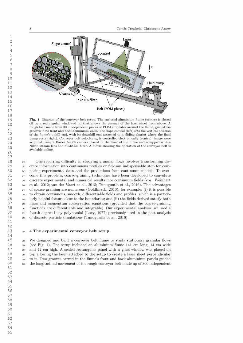
Fig. 1 Diagram of the conveyor belt setup. The enclosed aluminium flume (centre) is closedoff by a rectangular windowed lid that allows the passage of the laser sheet from above. Arough belt made from 300 independent pieces of POM circulates around the flume, guided viagrooves in its front and back aluminium walls. The slope control (left) sets the vertical positionof the flume’s uphill end, with its downhill end attached to a sliding chariot where the fluidpump rests (right). Conveyor belt velocity ub is controlled electronically (centre). Image wereacquired using a Basler A403k camera placed in the front of the flume and equipped with aNikon 28-mm lens and a 532-nm filter. A movie showing the operation of the conveyor belt isavailable online.
One recurring difficulty in studying granular flows involves transforming dis-241
crete information into continuous profiles or fieldsan indispensable step for com-242
paring experimental data and the predictions from continuum models. To over-243
come this problem, coarse-graining techniques have been developed to convolute244
discrete experimental and numerical results into continuum fields (e.g. Weinhart245
et al., 2012; van der Vaart et al., 2015; Tunuguntla et al., 2016). The advantages246
of coarse graining are numerous (Goldhirsch, 2010), for example: (i) it is possible247
to obtain continuous, smooth, differentiable fields and profiles, which is a particu-248
larly helpful feature close to the boundaries; and (ii) the fields derived satisfy both249
mass and momentum conservation equations (provided that the coarse-graining250
functions are differentiable and integrable). Our experimental analysis, we used a251
fourth-degree Lucy polynomial (Lucy, 1977) previously used in the post-analysis252
of discrete particle simulations (Tunuguntla et al., 2016).253
4 The experimental conveyor belt setup254
We designed and built a conveyor belt flume to study stationary granular flows255
(see Fig. 1). The setup included an aluminium flume 141 cm long, 14 cm wide256
and 42 cm high. A sealed rectangular panel with a glass window was placed on257
top allowing the laser attached to the setup to create a laser sheet perpendicular258
to it. Two grooves carved in the flume’s front and back aluminium panels guided259
the longitudinal movement of the rough conveyor belt made up of 300 independent260
1 2 3 4 5 6 7 8 9 10 11 12 13 14 15 16 17 18 19 20 21 22 23 24 25 26 27 28 29 30 31 32 33 34 35 36 37 38 39 40 41 42 43 44 45 46 47 48 49 50 51 52 53 54 55 56 57 58 59 60 61 62 63 64 65

Granular avalanches in a conveyor belt experimental setup 9
pieces and around four transversal aluminium rollers, with one pair located at each261
end of the aluminium flume. Each roller pair was arranged vertically to create walls262
that confined the granular material to the conveyed volume over the belt’s moving263
parts. The conveyed volume was 104 cm long, 10 cm wide, and 15 cm high. The264
aluminium flume had a glass window in the sidewall, parallel to the flow and265
compatible with image acquisition and the visualisation of the entire conveyed266
volume. A mixer was located behind the pair of rollers at each end of the flume’s267
aluminium structure to homogenise fluid. Various valves, beneath and above the268
setup, helped the processes of filling and emptying it.269
An analogue electro-mechanical system set the flume’s slope by vertically ad-270
justing the flume’s uphill end. The flume’s downhill end (fixed to a mobile cart)271
moved simultaneously in the horizontal direction. The slope could be adjusted to a272
wide range of values. Gentle or very steep slopes were inadvisable and impractical273
because particles might overflow the upper rollers and create mechanical issues.274
Each independent piece of the rough belt was a half-cylinder of polyoxymethy-275
lene (POM) screwed to an aluminium band. Roughness could be changed easily276
by replacing the POM half cylinders. For our experiments, we used a uniform277
roughness given by half cylinders of 4 mm in radius. Pieces were inserted into the278
grooves, next to each other, and were kept in place by the compression that the279
pieces applied against each other and were restrained vertically by the grooves.280
The conveyor belt was operated using a motor located behind the setup. The281
motor rotated the bottom uphill roller, whose geared wheel pushed the POM282
pieces along between the grooves in the sidepanels. Half of the pieces had two283
bolts beneath them so that the geared wheel could push against them and, move284
the belt. Pieces were alternately bolted and non-bolted to avoid breaking the285
geared wheel, the roller or the POM pieces. Motor speed was controlled using286
a dimmer switch that could apply a continuous range of belt velocities ub. The287
analogue controller did not give the ub value directly, and it had to be measured288
using a sensor that counted the motor axis revolutions as a function of time. These289
revolutions were then easily translated to a precise ub value using the radius of290
the geared wheel.291
The final setup was the outcome of a long, iterative process, which resulted292
in complex machinery that may be difficult to replicate. Although numerous dif-293
ficulties which arose during the construction were successfully solved, we failed to294
solve all of them (for other setup-related issues, see §7).295
5 Experimental dataset296
The conveyor belt was used to study the internal dynamics of granular flows made297
of monodisperse or bidisperse media. Conveyor belt velocity and slope were ad-298
justed so that stationary avalanches could be observed in the flume. Experiments299
were thus characterised by the slope θ and belt velocity ub (see Tab. 2). All the300
experiments presented here were carried out with the flume inclined at θ =15° to301
the horizontal.302
Two experiments were initially carried out using monodisperse beads to deter-303
mine a base state for later comparison with bidisperse experiments. The granular304
material used for these two runs was a 6-kg bulk of borosilicate beads of either305
ds = 6 or 8 mm diameter (see Experiments 1 and 6 in Tab. 2). We determined306
1 2 3 4 5 6 7 8 9 10 11 12 13 14 15 16 17 18 19 20 21 22 23 24 25 26 27 28 29 30 31 32 33 34 35 36 37 38 39 40 41 42 43 44 45 46 47 48 49 50 51 52 53 54 55 56 57 58 59 60 61 62 63 64 65

10 Tomas Trewhela, Christophe Ancey
Fig. 2 (a) Bulk’s solids volume fraction Φ, (b) longitudinal velocity field u and (c) verticalvelocity field w at t = 229.25 s for Experiment 1 (see Tab. 2). Longitudinal distances weremeasured from the wall formed by the POM pieces passing around the flume’s downhill par ofrollers. Two differing flow sections can be distinguished from the images with a sharp transitionat x ≈ -25 cm: (i) for x . -25 cm, a well-arranged particle flow flowing in layers, and; (ii) forx & -25 cm, a convective-bulged front where particles recirculate. The discontinuous linescorrespond to (b) vertical or (c) horizontal profiles of the velocity field. Velocity profile valuesare plotted using continuous white lines. These values are only shown to illustrate relativefluctuations along the profiles and visualise their shape. A movie of Experiment 1 is availableas supplementary material.
Table 2 Parameters of the experimental dataset. Φs is the overall small particle proportionof the bulk, the slope θ and the measured speed of the conveyor belt ub.
Experiment no. ds dl Φs (%) θ (°) ub (cms−1)
1 (monodisperse) 6 - 100 15 8.162 (bidisperse) 6 14 90 15 7.743 (bidisperse) 6 14 80 15 7.764 (bidisperse) 6 14 70 15 8.245 (bidisperse) 6 14 60 15 7.62
6 (monodisperse) 8 - 100 15 7.947 (bidisperse) 8 14 90 15 7.698 (bidisperse) 8 14 80 15 8.099 (bidisperse) 8 14 70 15 7.8210 (bidisperse) 8 14 60 15 8.16
bulk concentrations and velocity fields as functions of time. Next, we time-averaged307
these fields to obtain general trends and to describe processes that instantaneous308
frames were unable to show.309
The main body of experimental work consisted of eight stationary bidisperse310
granular avalanches. To include large particles in the bulk, we replaced part of the311
weight of small particles with large particles keeping the same total weight and only312
changed Φs. The overall general small particle concentration Φs, therefore, ranged313
from 90% to 60%, with the large particle concentration varying complementarily,314
i.e., Φl = 100− Φs. Since both species had the same intrinsic material density %∗,315
the overal bulk volume concentration remained the same in every run. In addition316
1 2 3 4 5 6 7 8 9 10 11 12 13 14 15 16 17 18 19 20 21 22 23 24 25 26 27 28 29 30 31 32 33 34 35 36 37 38 39 40 41 42 43 44 45 46 47 48 49 50 51 52 53 54 55 56 57 58 59 60 61 62 63 64 65

Granular avalanches in a conveyor belt experimental setup 11
to bulk concentrations and velocity fields, local volume concentrations of small317
particles φs and large particles φl = 1− φs were also determined from the images318
acquired using the coarse-graining technique (see §3.3) for experiments involving319
bidisperse media.320
Before data acquisition, the experiments were run until a stationary and, when321
possible, uniform flow was achieved. For each experiment, we first prepared the322
granular bulk of small and large particles (when needed) in the desired propor-323
tions. The particles were then put inside the flume and mixed as it rested almost324
horizontally. This resting position prevented particles from moving and altering325
their initial arrangement. We mixed the bulk before each experiment to have a326
close-to-homogeneous and reproducible initial condition. The fluid pump (shown327
in Fig. 1) was used to fill the flume with the interstitial fluid, and once full, we in-328
clined the flume and turned on the motor. Only after stationary flow condition was329
achieved, image acquisition could begin. The flow was considered stationary when330
the flow’s height profile and the avalanche front did not vary notably over sev-331
eral minutes. Image acquisition was performed for 5 minutes, and we took 12,000332
frames per run. The flume was then returned to a horizontal position and emptied333
before the next experiment.334
Due to the flume’s dimensions, the region of interest (ROI) for image acqui-335
sition did not cover the entire flume length. Our experimental images captured a336
length of 44 cm focused on the flow’s leading edge, near the downhill end of the337
flume. Thus, our experimental results involved 42% of the whole bulk. Full image338
acquisition of the entire avalanche would have implied lower image resolution, and339
the benefits in terms of physical insights would have been limited because the re-340
circulation of large particles in our experiments took place within the avalanche’s341
leading edge, whereas the unimaged flow behaved similarly to the flow in the ROI.342
5.1 Belt velocity343
We can consider ub as an input parameter or a measurement. Indeed, although344
ub was set before experimental image acquisition, its value varied with θ, the345
load on the belt and the friction imposed by the belt’s pieces. Many processes346
can alter motor torque and thereby belt velocity (see §4). Instead of calibrating347
of ub as a function of the electrical power supplied to the belt engine�a process348
fraught with uncertainties�we decided to measure its velocity directly after the349
desired stationary regime was achieved. Table 2 recaps the features of this work’s350
experimental dataset, with the measured ub values shown in the last column.351
6 Results352
6.1 Monodisperse experiments353
The monodisperse avalanches showed two distinctive flow sections: one at the front354
and the other at the back, with a marked transition between the two. Towards the355
flow front, at the flume’s downhill end, a convective, bulged region was observed.356
This front bulge was similar to that studied recently by Denissen et al. (2019) for a357
bidisperse flow. Henceafter, we refer to this region as the flow’s convective-bulged358
1 2 3 4 5 6 7 8 9 10 11 12 13 14 15 16 17 18 19 20 21 22 23 24 25 26 27 28 29 30 31 32 33 34 35 36 37 38 39 40 41 42 43 44 45 46 47 48 49 50 51 52 53 54 55 56 57 58 59 60 61 62 63 64 65

12 Tomas Trewhela, Christophe Ancey
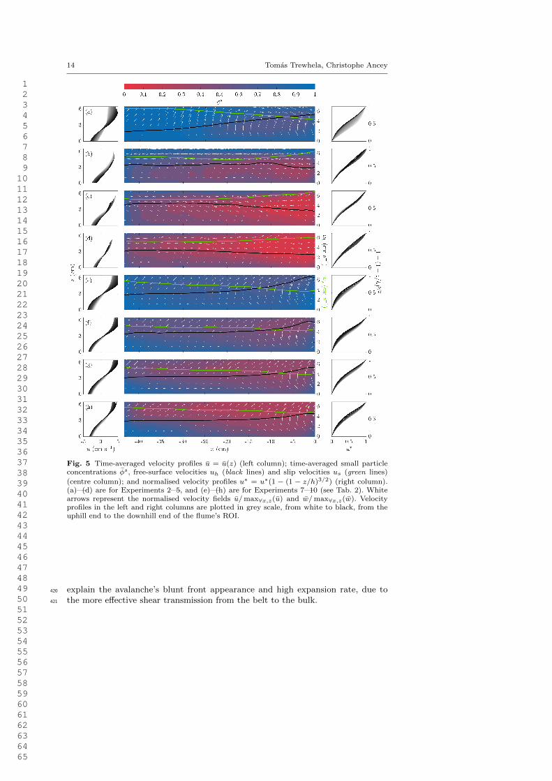
Fig. 3 Time-averaged velocity profiles u = u(z) (left column); time-averaged bulk’s solids
volume fraction field Φ, and free-surface velocity uh (black line) and slip us (green line) velocity
(centre column); and normalised velocity profiles u∗ = u∗(1−(1−z/h)3/2) (right column). Topand bottom rows show results for monodisperse 6-mm and 8-mm experiments (Experiments1 and 6 in Tab. 2, respectively). The velocity profiles are plotted in grayscale from white toblack, from the back to the front of the flow’s ROI, respectively.
front, or expanded front. In the rest of the conveyed volume, towards the flume’s359
uphill end, the particle flow transitioned into a well-arranged structure of particle360
layers that moved on top of each other. Naturally, this compact, ordered region361
was referred to as the layered flow. To illustrate these flow regions, Fig. 2 shows362
an experimental image and its corresponding extracted fields. This image was363
taken from Experiment 1 at t = 229.25 s, and its bulk volumetric concentration Φ,364
longitudinal (in the direction of the flow) velocity u and vertical velocity w fields365
are plotted on top of it. Fig. 2 reveals the particle structures in the background366
and a glimpse of the described flow regions. Overall bulk concentrations Φ varied367
between the described regions. The front showed a more diluted flow Φ ≈ 0.3,368
whereas the tail was more concentrated (Φ ≈ 0.5). The flow height h also showed369
marked differences, with height at the front reaching its maximum at h = 6 cm,370
or ≈ 10ds, whereas it was close to 4 cm at the back, or ≈ 7ds.371
To highlight some sections of the velocity field, we plotted profiles along the372
inclined flume’s longitudinal and transverse sections (see continuous white plots373
in Fig. 2(a) and (b)). The velocity field measurements revealed a quasi-uniform374
behaviour for u(z), with particles at the top moving faster than those at the375
bottom and a significant basal-slip condition, which was to be expected in such376
granular experiments (Louge and Keast, 2001; Ancey, 2001; Hsu et al., 2008).377
Vertical velocity w(x) profiles were notably less consistent along the flow, where378
we observed much more vertical particle movement in the flow’s leading edge than379
in its tail, where particle layers just moved on top of each other. As mentioned, the380
flow could be separated into two sections at x ≈ −25 cm, measured longitudinally381
from the flume’s downhill end. A sudden change of w ≈ 4cm s−1 marked the382
transition between the tail and leading-edge sections, from where particles started383
to recirculate within the bulged front. Only particles that had become tightly384
attached to the belt managed to escape the leading edge and, after reaching the385
flume’s uphill end, they were reincorporated into the avalanche.386
Time-averaged Φ, u and w fields were calculated to refine these general observa-387
tions. When time-averaged, velocity fields became smoother and the u(z) profiles388
showed consistent behaviour in the longitudinal direction. In general, these u(z)389
1 2 3 4 5 6 7 8 9 10 11 12 13 14 15 16 17 18 19 20 21 22 23 24 25 26 27 28 29 30 31 32 33 34 35 36 37 38 39 40 41 42 43 44 45 46 47 48 49 50 51 52 53 54 55 56 57 58 59 60 61 62 63 64 65

Granular avalanches in a conveyor belt experimental setup 13
Fig. 4 Time-averaged strain-rate tensor invariants in Experiment 1: (a) expansion rate IDand (b) shear rate IID . The vertical dashed lines correspond to vertical profiles and thecorresponding values for the strain-rate tensor invariants are plotted as continuous white lines.
profiles showed Bagnold-like characteristics, but subject to a strong basal slip us.390
Fig. 3 shows a normalised velocity profile u∗ defined as391
u∗ =u− u0uh − u0
(19)
where uh = u(h) is the surface particle velocity, and u0 = u(0) is the basal particle392
velocity, which in turn defined the slip velocity as the difference between belt speed393
and basal velocity, i.e. us = ub − |u0|. Therefore, u∗ is the time-averaged velocity394
field u normalised to the velocity difference between the base and the surface, and395
it is plotted as a function of 1−(1−z/h)3/2 (Fig. 3). We considered this expression396
for normalised velocity to show the influence of basal slip us on the overall velocity397
profile, which was negligible close to z = h. Close to the flow’s free-surface, most u∗398
profiles adjusted well to 1− (1− z/h)3/2, which is characteristic of a Bagnold-like399
profile (Bagnold, 1954; Silbert et al., 2001). In terms of longitudinal variation in400
the u∗ profiles, we saw that, towards the front, slip decreased and surface velocities401
increased (see us and uh in the centre-column subplots of Fig. 3). As a result, the402
u∗ profiles shown in Fig. 3’s right column subplots were in better agreement with403
the Bagnold scaling as we approached to the flow’s leading edge (darker lines are404
for vertical sections closer to the flume’s downhill end). However, at the very front405
of the flow, the agreement with the theoretical Bagnold profile decreased again.406
From a hydraulic point of view, this behaviour might be related to the changes in407
us, uh, and the free-surface profile.408
We determined the strain-rate tensor invariants to quantify how expanded409
or sheared the two flow regions were. Fig. 4 shows the time-averaged expansion410
rate ID and shear rate IID fields corresponding to the strain-rate tensor’s time-411
averaged first and second invariants (see §2.3). Our results indicated that the412
leading edge was highly-sheared and expanded, with a marked vertical gradient for413
ID and constant IID close to the front. To the rear, ID fluctuated around 0, and414
IID showed a negative gradient to the flow’s free-surface, with higher values at the415
bottom, as we would expect from the imposed boundary condition. Qualitatively,416
expansion and shear rates were significantly higher in regions where flow height417
was also high and Φ was low, right to the convective front. These observations were418
also related to low us values, as shown in Fig. 3. A decrease in basal slip might419
1 2 3 4 5 6 7 8 9 10 11 12 13 14 15 16 17 18 19 20 21 22 23 24 25 26 27 28 29 30 31 32 33 34 35 36 37 38 39 40 41 42 43 44 45 46 47 48 49 50 51 52 53 54 55 56 57 58 59 60 61 62 63 64 65
14 Tomas Trewhela, Christophe Ancey
Fig. 5 Time-averaged velocity profiles u = u(z) (left column); time-averaged small particleconcentrations φs, free-surface velocities uh (black lines) and slip velocities us (green lines)
(centre column); and normalised velocity profiles u∗ = u∗(1 − (1 − z/h)3/2) (right column).(a)�(d) are for Experiments 2�5, and (e)�(h) are for Experiments 7�10 (see Tab. 2). Whitearrows represent the normalised velocity fields u/max∀x,z(u) and w/max∀x,z(w). Velocityprofiles in the left and right columns are plotted in grey scale, from white to black, from theuphill end to the downhill end of the flume’s ROI.
explain the avalanche’s blunt front appearance and high expansion rate, due to420
the more effective shear transmission from the belt to the bulk.421
1 2 3 4 5 6 7 8 9 10 11 12 13 14 15 16 17 18 19 20 21 22 23 24 25 26 27 28 29 30 31 32 33 34 35 36 37 38 39 40 41 42 43 44 45 46 47 48 49 50 51 52 53 54 55 56 57 58 59 60 61 62 63 64 65

Granular avalanches in a conveyor belt experimental setup 15
Fig. 6 Segregation flux fsl for the Φs = 90 % experiment (Experiment 2, Tab. 2). fsl wascalculated using the formulation suggested by Trewhela et al. (2021a) and simplified in Eq.13.
6.2 Bidisperse experiments422
Adding large particles did not substantially change our avalanches’ overall dynam-423
ics. When the concentration of large particles was low (Φl = 10�20%), the leading424
edge concentrated those large particles, recirculating them. For Φl > 20%, the425
well-defined regions observed at low concentrations became less apparent, whereas426
other structures emerged. Large particles were often dragged uphill, past the tran-427
sition between the bulged-front and layered-tail regions, altering the characteristic428
structures observed in the monodisperse experiments. When we time-averaged the429
velocity and concentration fields, we still observed the convective leading edge. As430
a result of particle-size segregation, large particles were found predominantly at431
the free surface and within the leading edge, due to strong segregation fluxes in the432
middle of the bulk. This behaviour probably reflected a more effective transmission433
of shear close to the front, or low slip, which was observed in the monodisperse434
experiments.435
Figure 5 shows the time-averaged small particle concentration field φs for our436
experiments (Fig. 5, centre column). As expected from size segregation theory,437
the time-averaged concentration fields show an inversely-graded bulk towards the438
flume’s downhill end. We can infer from Fig. 5 that in experiments with larger439
R values (Experiments 2�5, (a)�(d) in Fig. 5), large particles recirculated within440
the flow’s leading edge. This large particle concentration resulted from a relatively441
faster segregation flux fsl for larger R values. To support this interpretation, we442
determined the segregation flux fsl using the empirical expression 13 (Fig. 6). For443
this calculation, we assumed a hydrostatic pressure distribution, and the φs and444
γ = 2IID fields were determined from coarse-grained experimental data. Results445
presented in Fig. 6 indicate that the segregation flux was highest in the convective-446
front region. This was closely connected with the shear-rate distribution shown in447
Fig. 4 for the monodisperse case, since fsl ∼ γ. The high values for fsl at the448
front were still smaller than the w values at the transition between flow regions,449
presented in Fig. 2 (w ≈ 4 cm s−1).450
Segregation-induced large-particle recirculation was observed in all the experi-451
ments and is shown via normalised velocities, u/max∀x,z(u) and w/max∀x,z(w), in452
the form of white arrows (Fig. 5, centre column). For R > 2, expansion rates were453
found to be related to more efficient, and hence faster, segregation rates (Trewhela454
et al., 2021b), which was evidenced by our large particles in Experiments 2�5. Our455
results for ds = 6 mm, i.e. R = 2.33, showed that large particles are probably to456
be constrained to the bulged-front, seen in Fig. 5 (a)�(d). For the experiments457
with R = 1.66 in Fig. 5 (e)�(h), we observed a less marked segregated state at458
1 2 3 4 5 6 7 8 9 10 11 12 13 14 15 16 17 18 19 20 21 22 23 24 25 26 27 28 29 30 31 32 33 34 35 36 37 38 39 40 41 42 43 44 45 46 47 48 49 50 51 52 53 54 55 56 57 58 59 60 61 62 63 64 65
16 Tomas Trewhela, Christophe Ancey
the front with lower large-particle concentrations, a sign that large particles were459
more homogeneously distributed along the flume.460
Breaking size segregation waves were observed in all the bidisperse avalanches.461
We can infer from Fig. 5 that the breaking-size segregation wave structure was462
similar to that observed by van der Vaart et al. (2018). From near the surface of463
the downstream end of the flow, large particles (red colour intensities in Fig. 5)464
fell onto the very front of the avalanche where they were overrun by the flow and465
dragged back into the bulk. Eventually, these large particles segregated and rose466
back to the surface onto the front, recirculating. The lens-shaped region (Gray467
and Ancey, 2009; Johnson et al., 2012; van der Vaart et al., 2018) where large and468
small particles were interchanged as a result of shear-induced segregation, can be469
seen in the middle part of the avalanche, between −40 < x < −10 cm for (a) to (h)470
in Fig. 5. Concentration gradients of φs in this region indicate an apparent mixing,471
where large particles rise and small particles percolate as a result of segregation.472
Our results also showed that changes in the overall particle concentrations between473
different experiments induced variations in the characteristics of the breaking-size-474
segregation waves. As we increased the overall concentration of large particles, they475
formed a thicker layer within the leading edge and the lens region extended uphill476
of the flow, disrupting the layered region described in §6.1.477
The results shown in Fig. 5 follow the trend observed in the monodisperse478
media experiments. Slip us was lower, with values that changed along the direction479
of the flow and ranged from 40% to 80% of ub (Fig. 5, green lines in centre480
column). From Fig. 5, we infer that the addition of large particles regularised slip481
by making the longitudinal gradient less steep than the low Φl and monodisperse482
media experiments. Surprisingly, the experiments with ds = 6 mm showed an483
inversion of the us profile when Φl was increased: a higher us was measured near the484
flow when Φl > 10%. However, this result was not consistent with the experiment485
made using ds = 8 mm, which suggests that bed roughness played an important486
part in shear transmission and should be considered when analysing the slip effect.487
Fig. 5’s right column shows that u∗ came close to 1− (1− z/h)3/2, indicating488
a Bagnold-like velocity profile (Bagnold, 1954; Mitarai and Nakanishi, 2005) for489
the bidisperse avalanches. Even though this result might have been expected, we490
found that velocity profiles were consistently uniform in shape. Similar to what491
was observed for monodisperse materials, basal slip tended to skew the profiles,492
particularly close to the belt, but further from the bottom, profiles were in good493
agreement with the Bagnold scaling. Average particle concentration influenced494
results in terms of consistency, as discussed: when Φl was increased, the slip all495
along the base became less variable and the velocity profiles matched the function496
1− (1− z/h)3/2.497
7 Conclusions498
Using a specially constructed inclined conveyor belt, we ran experiments to study499
granular avalanches. All ten experiments, carried out using monodisperse or bidis-500
perse media, exhibited a quasi-uniform steady behaviour characterised by a con-501
vective front at the downhill end of the inclined flume and a particle-layered tail502
towards the flume’s uphill end. Our experimental results revealed characteristics503
and structures typical of granular flows, which have been described in the lit-504
1 2 3 4 5 6 7 8 9 10 11 12 13 14 15 16 17 18 19 20 21 22 23 24 25 26 27 28 29 30 31 32 33 34 35 36 37 38 39 40 41 42 43 44 45 46 47 48 49 50 51 52 53 54 55 56 57 58 59 60 61 62 63 64 65

Granular avalanches in a conveyor belt experimental setup 17
erature. These features included blunt fronts (Denissen et al., 2019), breaking505
size-segregation waves (Thornton and Gray, 2008; Gray and Ancey, 2009; Johnson506
et al., 2012; van der Vaart et al., 2018) and crystallisation (Tsai and Gollub, 2004).507
Even for bidisperse media, time-averaged velocity profiles showed a h3/2 scaling508
consistent with Bagnold’s rheology and in agreement with earlier observations509
(Silbert et al., 2001; Mitarai and Nakanishi, 2005), and the µ(I) rheology (Jop510
et al., 2006). In this respect, the consistent behaviour exhibited by the u∗ profiles511
suggests the existence of an equivalent particle diameter dependent on dν and512
φν , as defined by Eq. (14) (Tripathi and Khakhar, 2011). Finally, these velocity513
profiles could be used as inputs to models coupling size segregation and granular514
avalanches as suggested by Gray and Ancey (2009). We moved a step further in515
that direction by computing the segregation flux fsl using the expression proposed516
by Trewhela et al. (2021a). We found that fsl was high within the avalanche’s517
leading edge, and this was further confirmed by large-particles recirculation and518
high values for both strain-rate tensor invariants (Trewhela et al., 2021b).519
Various velocity and slope conditions should be explored to identify similar-520
ities and differences with the results presented here. The influence of the belt’s521
roughness and the vertical boundaries created by the upper rollers could also be522
addressed, but eliminating their influence on the flow is currently impractical and523
outside this article’s scope. We believe that further work in that direction would524
not change the significance of the present experiments. Nonetheless, this experi-525
mental conveyor belt setup proved to be useful for the visualisation and study of526
the internal dynamics of granular flows.527
Acknowledgements We would like to thank the ENAC Technical Platform, particularly for528
the technical support, ideas, advice and time of Michel Teuscher, Joel Stoudmann and Bob de529
Graffenried, which were fundamental for the construction of this experimental setup.530
Kasper van der Vaart contributed in the conception of the setup’s initial prototype. The531
authors are thankful for their discussions about this article with N. M. Vriend, J. M. N. T.532
Gray and B. Lecampion.533
We acknowledge the Swiss National Science Foundation’s support through Project 200020 175750534
and the Swiss Federal Commission for Scholarships.535
Conflict of interest536
The authors declare that they have no conflict of interest.537
References538
Ancey, C. (2001). Dry granular flows down an inclined channel: Experimental539
investigations on the frictional-collisional regime. Phys. Rev. E, 65:011304.540
Ancey, C. and Evesque, P. (2000). Frictional-collisional regime for granular sus-541
pension flows down an inclined channel. Physical Review E, 62(6):8349.542
Bagnold, R. (1954). Experiments on a gravity-free dispersion of large solid spheres543
in a Newtonian fluid under shear. Proc. R. Soc. London, 225:49–63.544
Bai, K. and Katz, J. (2014). On the refractive index of sodium iodide solutions545
for index matching in piv. Experiments in fluids, 55(4):1704.546
1 2 3 4 5 6 7 8 9 10 11 12 13 14 15 16 17 18 19 20 21 22 23 24 25 26 27 28 29 30 31 32 33 34 35 36 37 38 39 40 41 42 43 44 45 46 47 48 49 50 51 52 53 54 55 56 57 58 59 60 61 62 63 64 65

18 Tomas Trewhela, Christophe Ancey
Barker, T., Rauter, M., Maguire, E. S. F., Johnson, C. G., and Gray, J. M. N. T.547
(2021). Coupling rheology and segregation in granular flows. Journal of Fluid548
Mechanics, 909:A22.549
Bridgwater, J., Foo, W., and Stephens, D. (1985). Particle mixing and segregation550
in failure zones — Theory and experiment. Powder Technol., 41:147–158.551
Budwig, R. (1994). Refractive index matching methods for liquid flow investiga-552
tions. Experiments in fluids, 17(5):350–355.553
Byron, M. L. and Variano, E. A. (2013). Refractive-index-matched hydrogel554
materials for measuring flow-structure interactions. Experiments in Fluids,555
54(2):1456.556
Chen, K. D., Lin, Y. F., and Tu, C. H. (2012). Densities, viscosities, refractive557
indexes, and surface tensions for mixtures of ethanol, benzyl acetate, and benzyl558
alcohol. Journal of Chemical & Engineering Data, 57(4):1118–1127.559
Clement, S. A., Guillemain, A., McCleney, A. B., and Bardet, P. M. (2018). Op-560
tions for refractive index and viscosity matching to study variable density flows.561
Experiments in Fluids, 59(2):32.562
Crocker, J. C. and Grier, D. G. (1996). Methods of digital video microscopy for563
colloidal studies. Journal of colloid and interface science, 179(1):298–310.564
Cui, M. M. and Adrian, R. J. (1997). Refractive index matching and marking meth-565
ods for highly concentrated solid-liquid flows. Experiments in Fluids, 22(3):261–566
264.567
Davies, T. (1988). Debris flow surges - A laboratory investigation. Technical Re-568
port Mitteilugen der Versuchanstalt fur Wasserbau, Hydrologie und Glaziologie569
n 96, Eidgenossischen Technischen Hochschule Zurich. 122 p.570
Davies, T. (1990). Debris-flow surges - Experimental simulation. J. Hydrol., 29:18–571
46.572
Deboeuf, S., Lajeunesse, E., Dauchot, O., and Andreotti, B. (2006). Flow rule,573
self-channelization, and levees in unconfined granular flows. Phys. Rev. Lett.,574
97:158303.575
Delannay, R., Valance, A., Mangeney, A., Roche, O., and Richard, P. (2017). Gran-576
ular and particle-laden flows: from laboratory experiments to field observations.577
J. Phys. D: Appl. Phys., 50:053001.578
Denissen, I. F. C., Weinhart, T., Te Voortwis, A., Luding, S., Gray, J. M. N. T.,579
and Thornton, A. R. (2019). Bulbous head formation in bidisperse shallow580
granular flow over an inclined plane. Journal of Fluid Mechanics, 866:263297.581
Dhillon, B. S. (2008). Mining Equipment Reliability, Maintainability, and Safety,582
chapter Mining Equipment Reliability, pages 57–70. Springer London, London.583
Dijksman, J., Rietz, F., Lorincz, K., and van Hecke, M. (2012). Refractive index584
matched scanning of dense granular materials. Rev. Sci. Instr., 83:011301.585
Dijksman, J. and van Hecke, M. (2010). Granular flows in split-bottom geometries.586
Soft Matter, 6:2901–2907.587
Dolgunin, V. and Ukolov, A. (1995). Segregation modeling of particle rapid gravity588
flow. Powder Technol., 83:95–103.589
Gajjar, P. and Gray, J. (2014). Asymmetric flux models for particle-size segregation590
in granular avalanches. J. Fluid Mech., 757:297–329.591
Gajjar, P., van der Vaart, K., Thornton, A. R., Johnson, C., Ancey, C., and Gray,592
J. (2016). Asymmetric breaking size-segregation waves in dense granular free-593
surface flows. J. Fluid Mech., 794:460–505.594
1 2 3 4 5 6 7 8 9 10 11 12 13 14 15 16 17 18 19 20 21 22 23 24 25 26 27 28 29 30 31 32 33 34 35 36 37 38 39 40 41 42 43 44 45 46 47 48 49 50 51 52 53 54 55 56 57 58 59 60 61 62 63 64 65
Granular avalanches in a conveyor belt experimental setup 19
Goldhirsch, I. (2010). Stress, stress asymmetry and couple stress: from discrete595
particles to continuous fields. Granular Matter, 12(3):239–252.596
Gray, J. (2018). Particle segregation in dense granular flows. Annu. Rev. Fluid597
Mech., 50:407–433.598
Gray, J. and Ancey, C. (2009). Segregation, recirculation and deposition at coarse599
particles near two-dimensional avalanche fronts. J. Fluid Mech., 629:387–423.600
Gray, J. and Thornton (2005). A theory for particle size segregation in shallow601
granular free-surface flows. Proc. R. Soc. London ser. A, 461:1447–1473.602
Hsu, L., Dietrich, W. E., and Sklar, L. S. (2008). Experimental study of bedrock603
erosion by granular flows. J. Geophys. Res., 113(F2).604
Iverson, R., Logan, M., and LaHusen, R. (2010). The Perfect Debris Flow? Aggre-605
gated Results from 28 Large-scale Experiments. J. Geophys. Res., 115:F03005.606
Johnson, C., Kokelaar, B., Iverson, R., Logan, M., LaHusen, R., and Gray, J.607
(2012). Grain-size segregation and levee formation in geophysical mass flows608
flows. J. Geophys. Res., 117:F01032.609
Jones, R. P., Isner, A. B., Xiao, H., Ottino, J. M., Umbanhowar, P. B., and Luep-610
tow, R. M. (2018). Asymmetric concentration dependence of segregation fluxes611
in granular flows. Physical Review Fluids, 3(9):094304.612
Jop, P., Pouliquen, O., and Forterre, Y. (2006). A constitutive law for dense613
granular flows. Nature, 441:727–730.614
Kokelaar, B., Graham, R., Gray, J., and Vallance, J. (2014). Fine-grained linings615
of leveed channels facilitate runout of granular flows. Earth Planet. Sci. Lett.,616
385:172–180.617
Li, J., Baird, G., Lin, Y.-H., Ren, H., and Wu, S.-T. (2005). Refractive-index618
matching between liquid crystals and photopolymers. Journal of the Society for619
Information Display, 13(12):1017–1026.620
Linares-Guerrero, E., Goujon, C., and Zenit, R. (2007). Increased mobility of621
bidisperse granular avalanches. J. Fluid Mech., 593:475–504.622
Louge, M. Y. and Keast, S. C. (2001). On dense granular flows down flat frictional623
inclines. Physics of Fluids, 13(5):1213–1233.624
Lucy, L. B. (1977). A numerical approach to the testing of the fission hypothesis.625
The astronomical journal, 82:1013–1024.626
Mangeney, A., Bouchut, F., Thomas, N., Vilotte, J.-P., and Bristeau, M. (2007).627
Numerical modeling of self-channeling granular flows and of their levee-channel628
deposits. J. Geophys. Res., 112:F02017.629
Mangeney, A., Roche, O., Hungr, O., Mangold, N., Faccanoni, G., and Lucas, A.630
(2010). Erosion and mobility in granular collapse over sloping beds. J. Geophys.631
Res., 115:F03040.632
Marks, B., Eriksen, J. A., Dumazer, G., Sandnes, B., and Mly, K. J. (2017). Size633
segregation of intruders in perpetual granular avalanches. Journal of Fluid Me-634
chanics, 825:502514.635
Martınez, F. J. (2008). Estudio experimental de flujos granulares densos. Master’s636
thesis.637
MiDi, G. D. R. (2004). On dense granular flows. The European Physical Journal638
E, 14(4):341–365.639
Mitarai, N. and Nakanishi, H. (2005). Bagnold scaling, density plateau, and kinetic640
theory analysis of dense granular flow. Physical review letters, 94(12):128001.641
Narrow, T., Yoda, M., and Abdel-Khalik, S. (2000). A simple model for the refrac-642
tive index of sodium iodide aqueous solutions. Experiments in fluids, 28(3):282–643
1 2 3 4 5 6 7 8 9 10 11 12 13 14 15 16 17 18 19 20 21 22 23 24 25 26 27 28 29 30 31 32 33 34 35 36 37 38 39 40 41 42 43 44 45 46 47 48 49 50 51 52 53 54 55 56 57 58 59 60 61 62 63 64 65

20 Tomas Trewhela, Christophe Ancey
283.644
Pane, S. F., Awangga, R. M., Azhari, B. R., and Tartila, G. R. (2019). Rfid-based645
conveyor belt for improve warehouse operations. Telkomnika, 17(2):794–800.646
Perng, A., Capart, H., and Chou, H. (2006). Granular configurations, motions, and647
correlations in slow uniform flows driven by an inclined conveyor belt. Granular648
Matter, 8(1):5–17.649
Poelma, C. (2020). Measurement in opaque flows: a review of measurement tech-650
niques for dispersed multiphase flows. Acta mechanica, 231:2089–2111.651
Pouliquen, O. (1999). Scaling laws in granular flows down rough inclined planes.652
Phys. Fluids, 11:542–548.653
Rocha, F., Johnson, C., and Gray, J. (2019). Self-channelisation and levee forma-654
tion in monodisperse granular flows. J. Fluid Mech., 876:591–641.655
Roche, O., Montserrat, S., Nino, Y., and Tamburrino, A. (2008). Experimental ob-656
servations of water-like behavior of initially fluidized, dam break granular flows657
and their relevance for the propagation of ash-rich pyroclastic flows. Journal of658
Geophysical Research: Solid Earth, 113(B12).659
Rousseau, G. and Ancey, C. (2020). Scanning piv of turbulent flows over and660
through rough porous beds using refractive index matching. Experiments in661
Fluids, 61(8):1–24.662
Saingier, G., Deboeuf, S., and Lagree, P.-Y. (2016). On the front shape of an663
inertial granular flow down a rough incline. Physics of Fluids, 28(5):053302.664
Sanvitale, N. and Bowman, E. T. (2012). Internal imaging of saturated granular665
free-surface flows. International Journal of Physical Modelling in Geotechnics,666
12(4):129–142.667
Sanvitale, N. and Bowman, E. T. (2016). Using piv to measure granular tem-668
perature in saturated unsteady polydisperse granular flows. Granular Matter,669
18(3):57.670
Savage, S. and Hutter, K. (1989). The motion of a finite mass of granular material671
down a rough incline. J. Fluid Mech., 199:177–215.672
Silbert, L., Ertas, D., Grest, G., Hasley, T., Levine, D., and Plimpton, S. (2001).673
Granular flow down an inclined plane: Bagnold scaling and rheology. Phys. Rev.674
E, 64:051302.675
Thomas, A. and Vriend, N. (2019). Photoelastic study of dense granular free-676
surface flows. Physical Review E, 100(1):012902.677
Thomas, N. and D’Ortona, U. (2018). Evidence of reverse and intermediate size678
segregation in dry granular flows down a rough incline. Physical Review E,679
97(2):022903.680
Thornton, A. and Gray, J. (2008). Breaking size segregation waves and particle681
recirculation in granular avalanches. J. Fluid Mech., 596:261–284.682
Trewhela, T., Ancey, C., and Gray, J. M. N. T. (2021a). An experimental scaling683
law for particle-size segregation in dense granular flows. Manuscript under review684
in Journal of Fluid Mechanics.685
Trewhela, T., Gray, J. M. N. T., and Ancey, C. (2021b). Large particle segregation686
in two-dimensional sheared granular flows. Manuscript under review in Physical687
Review Fluids.688
Tripathi, A. and Khakhar, D. (2011). Rheology of binary granular mixtures in the689
dense flow regime. Physics of Fluids, 23(11):113302.690
Tsai, J.-C. and Gollub, J. P. (2004). Slowly sheared dense granular flows: Crys-691
tallization and nonunique final states. Phys. Rev. E, 70:031303.692
1 2 3 4 5 6 7 8 9 10 11 12 13 14 15 16 17 18 19 20 21 22 23 24 25 26 27 28 29 30 31 32 33 34 35 36 37 38 39 40 41 42 43 44 45 46 47 48 49 50 51 52 53 54 55 56 57 58 59 60 61 62 63 64 65

Granular avalanches in a conveyor belt experimental setup 21
Tunuguntla, D. R., Thornton, A. R., and Weinhart, T. (2016). From discrete693
elements to continuum fields: Extension to bidisperse systems. Computational694
particle mechanics, 3(3):349–365.695
van der Vaart, K., Gajjar, P., Epely-Chauvin, G., Andreini, N., Gray, J., and696
Ancey, C. (2015). An underlying asymmetry within particle-size segregation.697
Phys. Rev. Lett., 114:238001.698
van der Vaart, K., Thornton, A. R., Johnson, C. G., Weinhart, T., Jing, L., Gajjar,699
P., Gray, J. M. N. T., and Ancey, C. (2018). Breaking size-segregation waves700
and mobility feedback in dense granular avalanches. Granular Matter, 20(3):46.701
Weinhart, T., Thornton, A. R., Luding, S., and Bokhove, O. (2012). From discrete702
particles to continuum fields near a boundary. Granular Matter, 14(2):289–294.703
Wiederseiner, S., Andreini, N., Epely-Chauvin, G., and Ancey, C. (2011). Re-704
fractive index matching in concentrated particle suspensions: A review. Exper.705
Fluids, 50:1183–1206.706
Appendix: Setup-related difficulties707
Plastic-fluid interactions708
Two important objectives of this setup were minimising the fluid volume used and709
the investigators’ exposure to harmful, flammable vapours; we therefore devised an710
enclosed flume. Achieving these objectives required sealing the setup to avoid leaks711
and spillages, which can be extremely dangerous when dealing with flammable712
fluids. Although this might seem simple at the outset, using non-conventional713
fluids led to interactions with the setup’s components. Sealing had to be done714
with plastics, but many of them reacted chemically with the ethanol and benzyl-715
alcohol mixture. For example, acrylics like poly (methyl methacrylate) (PMMA)716
were rapidly dissolved, and most rubbers lost some of their elastic properties�a717
feature fundamental for sealing. These materials had to be scrapped after a couple718
of hours or days of exposure to the fluid.719
Among plastics, polyoxymethylene (POM) and polyvinyl chloride (PVC) re-720
sisted long exposure to the fluid well. We observed no important changes in their721
material properties. However, and in general, these plastics are slightly porous and722
tend to absorb small amounts of fluid when immersed for a long time. Even though723
that absorption was very small, we noticed that after long use, friction between the724
belt pieces and the flume’s grooves increased to a point where the motor jammed.725
Not only did friction increase, but compression between the POM pieces became726
notably higher, which desynchronised them from the geared wheel. To determine727
how large the fluid absorption was, we measured the changes in length of two728
identical pieces of differing materials.729
Figure 7 shows measurements of two immersed belt pieces: one made of POM730
and one of PVC. Measurements were made after different fluid-exposure times, of731
up to 600 hours of submergence. To quantify the expansion, the material’s relative732
dilation was calculated as733
Relative dilation (%) =|Li − Li0|
Li0, (20)
1 2 3 4 5 6 7 8 9 10 11 12 13 14 15 16 17 18 19 20 21 22 23 24 25 26 27 28 29 30 31 32 33 34 35 36 37 38 39 40 41 42 43 44 45 46 47 48 49 50 51 52 53 54 55 56 57 58 59 60 61 62 63 64 65
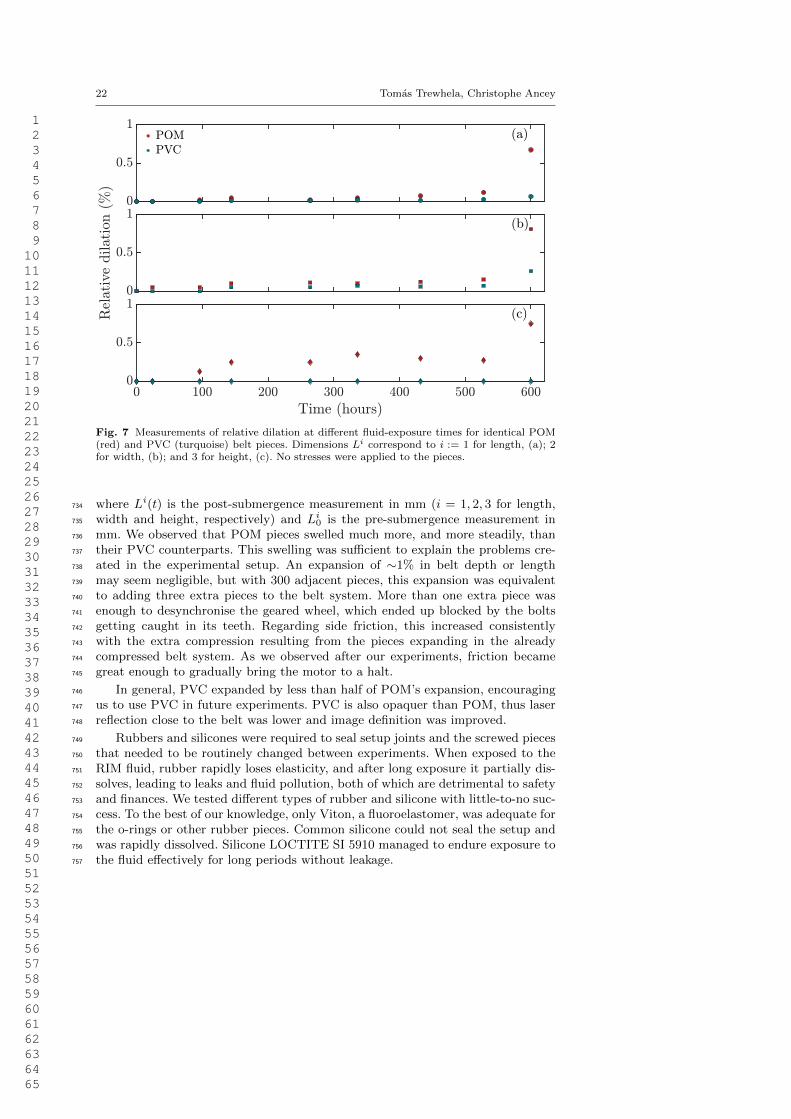
22 Tomas Trewhela, Christophe Ancey
Fig. 7 Measurements of relative dilation at different fluid-exposure times for identical POM(red) and PVC (turquoise) belt pieces. Dimensions Li correspond to i := 1 for length, (a); 2for width, (b); and 3 for height, (c). No stresses were applied to the pieces.
where Li(t) is the post-submergence measurement in mm (i = 1, 2, 3 for length,734
width and height, respectively) and Li0 is the pre-submergence measurement in735
mm. We observed that POM pieces swelled much more, and more steadily, than736
their PVC counterparts. This swelling was sufficient to explain the problems cre-737
ated in the experimental setup. An expansion of ∼1% in belt depth or length738
may seem negligible, but with 300 adjacent pieces, this expansion was equivalent739
to adding three extra pieces to the belt system. More than one extra piece was740
enough to desynchronise the geared wheel, which ended up blocked by the bolts741
getting caught in its teeth. Regarding side friction, this increased consistently742
with the extra compression resulting from the pieces expanding in the already743
compressed belt system. As we observed after our experiments, friction became744
great enough to gradually bring the motor to a halt.745
In general, PVC expanded by less than half of POM’s expansion, encouraging746
us to use PVC in future experiments. PVC is also opaquer than POM, thus laser747
reflection close to the belt was lower and image definition was improved.748
Rubbers and silicones were required to seal setup joints and the screwed pieces749
that needed to be routinely changed between experiments. When exposed to the750
RIM fluid, rubber rapidly loses elasticity, and after long exposure it partially dis-751
solves, leading to leaks and fluid pollution, both of which are detrimental to safety752
and finances. We tested different types of rubber and silicone with little-to-no suc-753
cess. To the best of our knowledge, only Viton, a fluoroelastomer, was adequate for754
the o-rings or other rubber pieces. Common silicone could not seal the setup and755
was rapidly dissolved. Silicone LOCTITE SI 5910 managed to endure exposure to756
the fluid effectively for long periods without leakage.757
1 2 3 4 5 6 7 8 9 10 11 12 13 14 15 16 17 18 19 20 21 22 23 24 25 26 27 28 29 30 31 32 33 34 35 36 37 38 39 40 41 42 43 44 45 46 47 48 49 50 51 52 53 54 55 56 57 58 59 60 61 62 63 64 65

Granular avalanches in a conveyor belt experimental setup 23
Pollutants and filtering system758
The conveyor belt pieces inevitably produced friction between themselves, the759
grooves and the rollers. Most of the friction was against aluminium and the scrap-760
ing released a very fine black dust that spreads throughout the setup. Long-running761
experiments accumulated enough dust to reduce fluid transparency, obstructing762
the laser and reducing image quality. To enhance image definition and increase763
light intensity, we changed acquisition parameters, like the gain and/or reduced764
the lens’ focal ratio. Nevertheless, the black dust concentration would increase to765
a point where these improvements became pointless.766
A filtering system was devised to remove the dust from the fluid. We could767
have used a wet sieving/filtering system, such as a Retsch AS200, but knowing768
nothing about its components and not wanting to damage it with exposure to our769
fluid, we decided to try a simpler method. A large reservoir dripped fluid into a770
funnel containing 40 µm filter paper. We were able to filter the fluid entirely in771
approximately one day, which was a reasonable amount of time in which to prepare772
the next experiment. With twice the amount of fluid, we were able to rotate the773
fluid batches and keep the amount of dust under control, thus not harming image774
quality. A reduction in dust production, via improvements such as stainless steel775
grooves, could certainly enhance the setup’s performance and image quality in the776
future, but these were not used for this work.777
1 2 3 4 5 6 7 8 9 10 11 12 13 14 15 16 17 18 19 20 21 22 23 24 25 26 27 28 29 30 31 32 33 34 35 36 37 38 39 40 41 42 43 44 45 46 47 48 49 50 51 52 53 54 55 56 57 58 59 60 61 62 63 64 65


![1 SERIES Belt Conveyor System B090 - Bett Sistemi Srl€¦ · CONVEYOR BELT DEVELOPMENT CALCULATION FORMULA Conveyor belt length = 300 + {[(L-94)-(2• Conveyor belt thick. )]•2}](https://img.pdfslide.net/doc/110x75/5ad3c4047f8b9a48398b7ae4/1-series-belt-conveyor-system-b090-bett-sistemi-conveyor-belt-development-calculation.jpg)