A copula–GARCH model for macro asset allocation of a portfolio with commodities

Empir EconDOI 10.1007/s00181-012-0577-1

A copula–GARCH model for macro asset allocationof a portfolio with commoditiesAn out-of-sample analysis

Luca Riccetti

Received: 23 August 2011 / Accepted: 12 December 2011© Springer-Verlag 2012

Abstract Many authors have suggested that the mean-variance criterion, conceivedby Markowitz (The Journal of Finance 7(1):77–91, 1952), is not optimal for asset allo-cation, because the investor expected utility function is better proxied by a function thatuses higher moments and because returns are distributed in a non-Normal way, beingasymmetric and/or leptokurtic, so the mean-variance criterion cannot correctly proxythe expected utility with non-Normal returns. In Riccetti (The use of copulas in assetallocation: when and how a copula model can be useful? LAP Lambert, Saarbrücken2010), a copula–GARCH model is applied and it is found that copulas are not usefulfor choosing among stock indices, but can be useful in a macro asset allocation model,that is, for choosing stock and bond composition of portfolios. In this paper I applythat copula–GARCH model for the macro asset allocation of portfolios containing acommodity component. I find that the copula model appears to be useful and betterthan the mean-variance one for the macro asset allocation also in presence of a com-modity index, even if it is not better than GARCH models on independent univariateseries, probably because of the low correlation of the commodity index returns to thestock, the bond and the exchange rate returns.

Keywords Commodities · Portfolio choice · Asset allocation · Copula · GARCH

JEL Classification C52 · C53 · C58 · G11 · G17

L. Riccetti (B)Department of Social and Economics Sciences, Università Politecnica delle Marche, P.le Martelli 8,60121 Ancona, Italye-mail: [email protected]

123

L. Riccetti

1 Introduction

In Riccetti (2010), a copula–GARCH model appears useful for macro asset alloca-tion (choosing stock and bond composition of portfolios), while it is not useful whenchoosing of the weights for a portfolio composed of many stock indices. A possibledriving factor of the performance of the copula model is the correlation value betweenthe assets: the copula model appears to be useful in the case of a portfolio containingone asset with small absolute values of correlation, while this model is dangerous withhighly correlated assets.

In this paper, I want to check if that good result of the copula model is confirmedin a portfolio containing a commodity index, that is uncorrelated with the stock index,the bond index and the exchange rate returns time series. I also extend the analysisdone in Riccetti (2010) in two parts:

– analysing portfolios composed by three and four assets that are all uncorrelated;– adding the comparison of the copula model to one that implies independent assets.

Moreover, this is a relevant topic for real asset management, indeed in recent yearsthe investments in commodities continue to increase, also thanks to the recent creationof a number of financial vehicles (exchange traded funds or mutual funds), that makethe investment in commodities possible for retail investors too.

The paper proceeds as follows. This section briefly reviews some papers aboutthe use of commodities and copulas in the asset allocation context, especially witha review of the book by Riccetti (2010), that is the base for the following analysis;Sect. 2 presents the model; Sect. 3 reports the results and Sect. 4 concludes.

1.1 Use of commodities

Authors such as Irwin and Landa (1987); Froot (1995); Abanomey and Mathur (1999);Jensen et al. (2000, 2002); Gorton and Rouwenhorst (2006); Dempster and Artigas(2010) or Conover et al. (2010) found that commodities offer sizeable diversificationbenefits in the portfolio allocation, especially in equity portfolios, because their returnsare uncorrelated to the stock returns.1

Many papers, such as Bodie (1983); Halpern and Warsager (1998); Gorton andRouwenhorst (2006); Amenc et al. (2009) or Dempster and Artigas (2010), explainthat the low correlation appears to be driven by the returns of the commodities inperiods of high inflation (expected or not): in these periods, while stock or bond port-folios are negatively affected, commodities provide a hedge against inflation, thus thediversification benefit is coupled by a return benefit. These papers also often highlightthat high inflation periods coincide with periods in which the central banks apply a

1 Moreover, there is debate on the utility of commodity during extreme events: Chong and Miffre (2010)find that the correlations between the S&P500 index and several commodities fell in periods of above-aver-age volatility in equity markets, while Büyüksahin et al. (2010) find that correlations between equity andcommodity returns increased sharply in the fall of 2008, so diversification benefits are weaker when theyare needed most. On this debate, see also Appendix B. Copula models could catch the extreme outcomefeatures.

123

A copula–GARCH model for macro asset allocation

restrictive monetary policy and so, as in Jensen et al. (2000) or Conover et al. (2010),they show that the allocation can be improved using the information given by themonetary policy (that is to invest more in commodities during restrictive monetaryphases and vice versa).

The growing interest in commodities makes the financial engineering developinvestment vehicles to give the opportunity to retail investors to allocate part oftheir portfolios in commodities without using futures. Indeed, in recent years a lotof exchange traded funds (ETFs) and mutual funds have been introduced, as shown inpapers like Mazzilli and Maister (2006); Anderson (2008) or Conover et al. (2010).Moreover, authors such as Amenc et al. (2009) or Dempster and Artigas (2010), pointout that today the financial crisis drives central banks to lower interest rates and topump a lot of money into the economy, so there is the risk of a rise in inflation that couldbe hedged by commodities which are likely to outperform stock and bond returns inthese periods. This is the reason for the increasing interest in commodities.

1.2 Use of copulas

The Markowitz model is optimal if investors only care about mean and variance or ifreturns are distributed as a Normal.

In fact, on one hand, financial returns are not Normally distributed, as observedsince 1963 in two papers by Mandelbrot and Fama.

On the other hand, many authors like Arditti (1967); Kraus and Litzenberger(1976); Simkowitz and Beedles (1978) found, for example, that people prefer highvalues for skewness. Scott and Horvath (1980) analytically prove that investors preferreturns with higher skewness and lower kurtosis. This proof is also repeated for highermoments and people always prefer higher values for odd moments and lower valuesfor even moments.

Many authors, such as Harvey and Siddique (2000) and Dittmar (2002), prove thathigher moments improve the allocation if returns are distributed in a very differentway from the Normal.

Copulas are a very useful tool to deal with non standard multivariate distribution. Acopula is a function that represents the dependency structure of a multivariate randomvariable. Sklar (1959) shows that all multivariate distribution functions contain copulasand that copulas may be used in conjunction with univariate distribution functions toconstruct multivariate distribution functions. Indeed, every joint distribution functioncontains a description of the marginal behaviour of the individual factors, given by theunivariate distribution, and a description of their dependence structure, given by thecopula. Copulas isolate the description of the dependence, and help to understand it ata deeper level than correlation, describing the dependence on a quantile scale. In thisway, they can describe the extreme outcomes and allow the building of a multivariatemodel, that combines more developed marginal models with the variety of dependencemodels. For a deep introduction on copulas see Embrechts et al. (2005) or Joe (1997).

Over recent years, many authors have applied copulas to financial research. Muchliterature exists on the use of copulas for the computation of Value-at-Risk (VaR) inrisk management and very advanced papers have been published in this field. How-

123

L. Riccetti

ever, there are also papers that use copulas to model stock market returns without adirect application to risk management, as in Jondeau and Rockinger (2006a) and inSun et al. (2009), where the authors investigate respectively the bivariate interactionsbetween four major stock indices (S&P500, FTSE100, DAX, CAC) and the multi-variate interaction among nine stock indices and both find that the Student-t copulais more accurate than the Gaussian one, consistent with the idea that dependence isstronger in the tails.

Although the wide use of copulas in finance, very few works, such as Patton (2004);Sun et al. (2008); Riccetti (2010), and Rachev et al. (2011), assess the effectivenessof this tool in the out-of-sample forecast.

Patton (2004) is the first paper that builds an asset allocation with copulas. He workson a portfolio composed by two assets (a basket of stocks with low market capital-ization and a basket of stocks with high market capitalization), evaluating the assetallocation in terms of investor’s utility. Patton, using monthly returns, tries some mod-els with different copulas (Normal, Student-t, Clayton, rotated Clayton, Joe-Clayton,Plackett, Frank, Gumbel and rotated Gumbel copulas) and selects the rotated Gumbelcopula that obtains the best information criteria values. He finds that the model thatapplies the Skewed-t marginal distribution and the rotated Gumbel copula gains moreutility, especially if the investor is very risk averse, compared to other allocationsbased on naive strategies or on bivariate Normal distribution or on the Normal copulaassumption.

Sun et al. (2008) analyse the out-of-sample prevision of some copula ARMA–GARCH models to forecast the co-movements of six German equity market indicessampled at high-frequency.2 The authors, using some goodness-of-fit tests, find thatthe copula ARMA–GARCH model is able to capture the multi-dimensional co-move-ments among the indices. In particular, they compare six kinds of distributions (whitenoise, fractional Gaussian noise, Lévy fractional stable noise, Lévy stable distribution,generalized Pareto distribution and generalized extreme value distribution) to modelthe GARCH residuals, and three copulas (Normal, Student-t and Skewed-t), findingthat Skewed-t copula with Lévy fractional stable ARMA–GARCH model has the bestresults: the Skewed-t copula is able to capture asymmetric co-movements, while theLévy fractional stable ARMA–GARCH model is able to capture marginal univariatefeatures such as long-range dependence, excess kurtosis and volatility clustering.

Riccetti (2010) develops the analysis published by Patton (2004). The modelsuse different copulas (Normal, Student-t, Clayton, Gumbel, Frank, mix copulas andCanonical Vine copulas) in an allocation of two, three and four assets, analyzing vari-ous combinations of indices, to test whether the use of copulas improves the investor’sutility and revenue. Using daily data and monthly or weekly portfolio rebalancing,those analyses conclude that the best copula model is the one that uses the Student-tcopula, but the copula model is better than the naive allocations and than the mean–variance model only for deciding the macro-asset allocation (for choosing the stockand the bond composition of the portfolios) or when the portfolio is composed by one

2 Sun et al. (2008) use high-frequency data to overcome the ‘breakdown of the permanence hypothesis’(that is the composition changes of stock indices) still having a large amount of observation, not to lose theintra-daily co-movements, and to capture both microstructure effects and macroeconomic factors.

123


bond index and more stock indices, especially when the investor is very risk averse.Instead, the copula model is not useful neither in the choice between some differentstock indices in portfolios composed only by equity, nor in the choice of the weightsof portfolios composed by two stock indices and two bond indices. It is argued that apossible driving factor of the performance of the copula model is the correlation valuesbetween the assets: when there is one index that has small absolute values of corre-lation with all the other indices, then the copula model appears to be useful. Besides,Riccetti (2010) finds that, when the number of assets increases, the standard copulamodel shows increasing problems and the use of Vine copulas (see Appendix A) canreduce these problems, even if they are still present.

Rachev et al. (2011), in chapter 10 of their book, provide an analysis on the per-formance of a portfolio allocation on 30 German stocks with daily data and weeklyportfolio rebalancing. They propose a different methodology with a multifactor linearmodel to reduce the problem of dimensionality, applying on these factors a Skewed-t copula ARMA(1,1)–GARCH(1,1) model with standard classical tempered stablemarginal distributions. Moreover, Rachev et al. (2011) select portfolio weights thatmaximize the ratio between the expected excess return over the benchmark and theaverage Value-at-Risk (AVaR or expected shortfall) and not the investor’s expectedutility as in Patton (2004) or Riccetti (2010). They evaluate the out-of-sample perfor-mance with the Sharpe ratio and with the stable tail-adjusted return ratio (that is theexcess return divided by the AVaR) finding that the proposed model performs betterthan the mean–variance one.

2 Data and model

To build the model I make some simplifying assumptions. I assume that the investordoes not face any transaction costs, so there are no costs for rebalancing or for short-selling. Moreover, I take exogenously specified savings decisions and ignore inter-mediate consumption: the investor/asset manager has to invest an amount of moneyat the beginning of the period (that, for simplicity, I take as equal to 1) and does notreceive or disinvest anything until the end.3 The allocation is done for three yearsleft out-of-sample, with a monthly rebalancing, so there are 36 rebalancings every 22working days (I assume that a month has 22 working days).

The assets used for the analysis are four: a commodity index (the New York CRB),a stock index (the Dow Jones Industrial), a bond index (the Merrill Lynch US Treasury1–10 years) and the exchange rate between US Dollar and Euro. I use daily log returnsfor all assets. Differently from Patton, who uses monthly returns, daily returns areused in the present analysis, but I aim to obtain monthly allocations. In this way, Icover quite a long time period without rebalancing (and this reduces the problem of notconsidering rebalancing costs), but I use more information compared to few monthlyreturns.4 However, to do this, I need to simulate a path of 22 returns to allocate theportfolio for each out-of-sample month, as I will explain after.

3 As remarked by Ang and Bekaert (2002), the use of a CRRA utility function does not address marketequilibrium, so the investor does not necessarily have to be the representative agent.4 Similar to Morana (2009), who computes monthly realized betas from daily data.

123

L. Riccetti

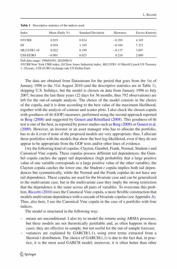
Table 1 Descriptive statistics of the indices used

Index Mean (Daily %) Standard Deviation Skewness Excess Kurtosis

NYCRB 0.019 0.824 −0.283 4.345

DJ 0.018 1.245 −0.104 7.223

MLUSTR1-10 0.022 0.199 −0.137 3.897

US$-EURO −0.001 0.623 0.216 2.880

Full data range: 1996/01/01–2010/08/31NYCRB New York CRB index, DJ Dow Jones Industrial index, MLUSTR1-10 Merrill Lynch US Treasury1–10 years, US$-EURO exchange rate US Dollar-Euro

The data are obtained from Datastream for the period that goes from the 1st ofJanuary 1996 to the 31st August 2010 (and the descriptive statistics are in Table 1),skipping U.S. holidays, but the model is chosen on data from January 1996 to July2007, because the last three years (22 days for 36 months, thus 792 observations) areleft for the out-of-sample analysis. The choice of the model consists in the choiceof the copula, and it is done according to the best value of the maximum likelihood,together with the analysis of contour and scatter plots. I also check the chosen copulawith goodness-of-fit (GOF) measures, performed using the second approach reportedin Berg (2008) and suggested by Genest and Rémillard (2008). This goodness-of-fittest is one of the best, as reported by power studies such as Berg (2008) or Genest et al.(2009). However, an investor or an asset manager who has to allocate the portfolio,has to do it even if none of the proposed models are very appropriate; thus, I allocatethese portfolios with the models that show the best log-likelihood, even if they do notappear to be appropriate from the GOF tests and/or other lines of evidence.

I try the following kind of copulas: Clayton, Gumbel, Frank, Normal, Student-t andCanonical Vine copula. These copulas possess different tail dependences: the Gum-bel copula catches the upper tail dependence (high probability that a large positivevalue of one variable corresponds to a large positive value of the other variable), theClayton copula catches the lower one, the Student-t copula implies both tail depen-dences but symmetrically, while the Normal and the Frank copulas do not have anytail dependence. These copulas are used for the bivariate case and can be generalizedto the multivariate case, but in the multivariate case they imply the strong restrictionthat the dependence is the same across all pairs of variables. To overcome this prob-lem, Riccetti (2010) uses the Canonical Vine copula, a more flexible construction thatmodels multivariate dependence with a cascade of bivariate copulas (see Appendix A).Thus, also here, I use the Canonical Vine copula in the case of a portfolio with fourindices.

The model is structured in the following way:

– means are unconditional. I also try to model the returns using ARMA processes,but these models are not theoretically justifiable and, as often happens in thesecases, they are effective in-sample, but not useful for the out-of-sample forecast;

– variances are explained by GARCH(1,1), using error terms extracted from aSkewed-t distribution. The choice of GARCH(1,1) is due to the fact that, in prac-tice, it is the most used GARCH model; moreover, it is often better than other

123


(more complex) GARCH models for the out-of-sample forecast. The error termsare extracted from a Skewed-t distribution, as presented by Patton (2004) or byJondeau and Rockinger (2003), because all GARCH residuals present negativeskewness and excess kurtosis. However, differently from the above cited papers,skewness and kurtosis parameters are non conditional;

– the joint behaviour of the residuals of the indices is modelled by the copula thatpresents the best log-likelihood.

The steps to build the optimal portfolio are:

1. estimate with the Maximum Likelihood the parameters of the above model;2. simulate the path of assets returns on the investment horizon (22 days) 5,000 times;3. choose the optimal weights in order to maximize the investor’s expected utility,

using the CRRA utility function as done, for instance, in Patton (2004):

U (γ ) = (1 − γ )−1(P0 Rport )1−γ (1)

with γ is the risk aversion parameter, Rport is the portfolio capitalization factor,and P0=1 is the initial investment. The values of γ used are: 2, 5, 10 and 15, assuggested by Bucciol and Miniaci (2008) and such as chosen by other authors (forexample Jondeau and Rockinger (2006b)).

In the next section, I report the result of the copula model compared to the mean–var-iance model, to a model that supposes all series to be independent and to an allocationequally divided among the assets, that is used as a benchmark. With the use of theCRRA utility function, I cannot derive a simple closed form for the optimal weightsin Markowitz; so I use, as an approximation of the weight for the mean–varianceapproach, a model that uses GARCH(1,1) for the univariate variances and shocksextracted from a multivariate Normal with correlations equal to the in-sample histor-ical ones.

I use the final amount of the portfolio and the utility obtained by the monthly returns,to compare the allocations. To compare the utility I use the management fee, calledalso opportunity cost or forecast premium, that is the amount that the investor wouldpay to switch from the equally divided portfolio (that does not use any information)to the analysed allocation. In other words, it is the return that needs to be added tothe returns obtained by the equally divided portfolio, so that the investor becomesindifferent to the returns obtained by the analysed model. Formally, denoting r∗

p as theoptimal portfolio return obtained by the copula or the Markowitz or the independencemodel, and denoting rp as the return obtained by the equally divided portfolio, theopportunity cost θ is:

U (1 + rp + θ) = U (1 + r∗p) (2)

Following an approach similar to Jondeau and Rockinger (2006b) in the context of afourth-order Taylor approximation with CRRA utility function, the previous equationcan be written as follows:

123

L. Riccetti

θ = (μ∗p − μp) − γ

2(m∗2

p − m2p) + γ (γ + 1)

3! (m∗3p − m3

p)

−γ (γ + 1)(γ + 2)

4! (m∗4p − m4

p) (3)

where μ represents the mean return and m represents the non central moments: mip =

mean[r ip].

I use this expression to calculate the forecast premium. It indicates that the investoris willing to pay to use a strategy that decreases variance and kurtosis and increasesmean and skewness of his/her portfolio returns.

3 Results

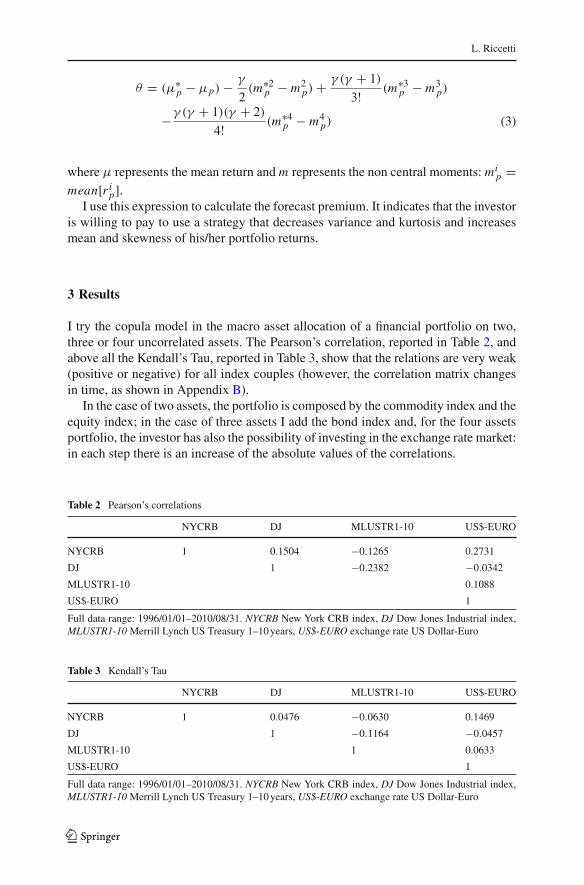
I try the copula model in the macro asset allocation of a financial portfolio on two,three or four uncorrelated assets. The Pearson’s correlation, reported in Table 2, andabove all the Kendall’s Tau, reported in Table 3, show that the relations are very weak(positive or negative) for all index couples (however, the correlation matrix changesin time, as shown in Appendix B).

In the case of two assets, the portfolio is composed by the commodity index and theequity index; in the case of three assets I add the bond index and, for the four assetsportfolio, the investor has also the possibility of investing in the exchange rate market:in each step there is an increase of the absolute values of the correlations.

Table 2 Pearson’s correlations

NYCRB DJ MLUSTR1-10 US$-EURO

NYCRB 1 0.1504 −0.1265 0.2731

DJ 1 −0.2382 −0.0342

MLUSTR1-10 0.1088

US$-EURO 1

Full data range: 1996/01/01–2010/08/31. NYCRB New York CRB index, DJ Dow Jones Industrial index,MLUSTR1-10 Merrill Lynch US Treasury 1–10 years, US$-EURO exchange rate US Dollar-Euro

Table 3 Kendall’s Tau


NYCRB 1 0.0476 −0.0630 0.1469

DJ 1 −0.1164 −0.0457

MLUSTR1-10 1 0.0633

US$-EURO 1

Full data range: 1996/01/01–2010/08/31. NYCRB New York CRB index, DJ Dow Jones Industrial index,MLUSTR1-10 Merrill Lynch US Treasury 1–10 years, US$-EURO exchange rate US Dollar-Euro

123


3.1 Two assets: equity and commodity portfolio

I begin with the portfolio composed by the Dow Jones Industrial index and the NewYork CRB index.

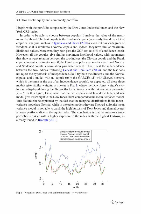
In order to be able to choose between copulas, I analyse the value of the maxi-mum likelihood. The best copula is the Student-t copula (as already found by a lot ofempirical analysis, such as in Ignatieva and Platen (2010)), even if it has 75 degrees offreedom, so it is similar to a Normal copula and, indeed, they have similar maximumlikelihood values. Moreover, they both pass the GOF test (at 5 % of confidence level).However, all the copulas give similar maximum likelihood values, with parametersthat show a weak relation between the two indices: the Clayton copula and the Frankcopula present a parameter near 0, the Gumbel copula a parameter near 1 and Normaland Student-t copula a correlation parameter near 0. Thus, I test the independencebetween the two indices, following Genest and Rémillard (2004), and the test doesnot reject the hypothesis of independence. So, I try both the Student-t and the Normalcopulas and a model with no copula (only the GARCH(1,1) with Skewed-t errors,which is the same as the use of an Independence copula). As expected, all these threemodels give similar weights, as shown in Fig. 1, where the Dow Jones weight’s evo-lution is displayed during the 36 months for an investor with risk aversion parameterγ = 5. In this figure, I also note that the two copula models and the Independencemodel give less weight to the Dow Jones index compared to the mean–variance model.This feature can be explained by the fact that the marginal distributions in the mean–variance model are Normal, while in the other models they are Skewed-t. So, the meanvariance model is not able to catch the high kurtosis of Dow Jones and then allocatesa larger portfolio slice to the equity index. The conclusion is that the mean–varianceportfolio is riskier with a higher exposure to the index with the highest kurtosis, asalready found in Riccetti (2010).

month

wei

ght

0 5 10 15 20 25 30 35

0.0

0

.5

1.0

1.5 circle: Student−t copula model

square: Normal copula modelrhombus: Independence modeltriangle: Mean−variance model

Fig. 1 Weights of Dow Jones with different models—γ = 5 investor

123

L. Riccetti

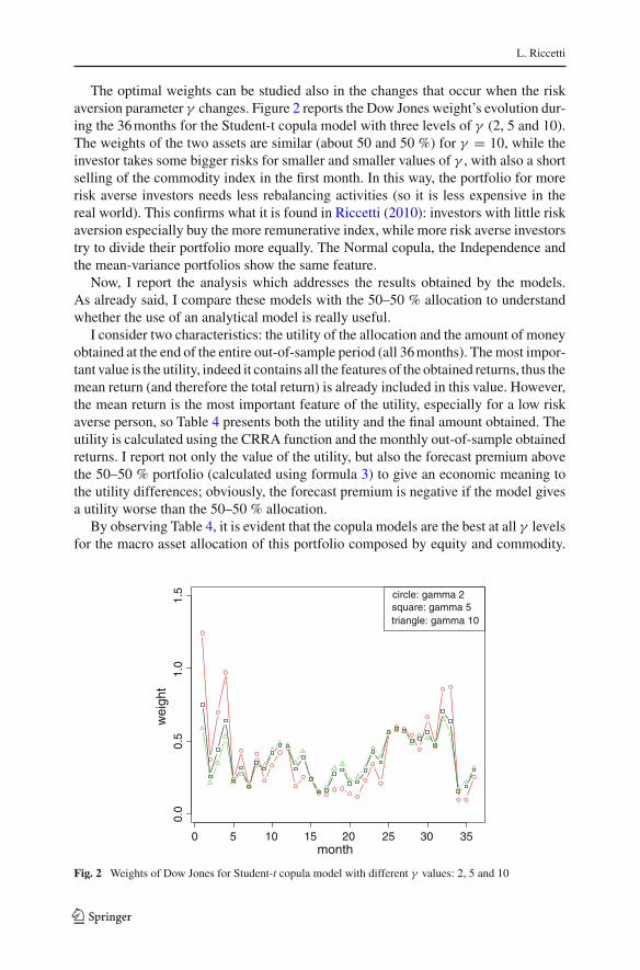
The optimal weights can be studied also in the changes that occur when the riskaversion parameter γ changes. Figure 2 reports the Dow Jones weight’s evolution dur-ing the 36 months for the Student-t copula model with three levels of γ (2, 5 and 10).The weights of the two assets are similar (about 50 and 50 %) for γ = 10, while theinvestor takes some bigger risks for smaller and smaller values of γ , with also a shortselling of the commodity index in the first month. In this way, the portfolio for morerisk averse investors needs less rebalancing activities (so it is less expensive in thereal world). This confirms what it is found in Riccetti (2010): investors with little riskaversion especially buy the more remunerative index, while more risk averse investorstry to divide their portfolio more equally. The Normal copula, the Independence andthe mean-variance portfolios show the same feature.

Now, I report the analysis which addresses the results obtained by the models.As already said, I compare these models with the 50–50 % allocation to understandwhether the use of an analytical model is really useful.

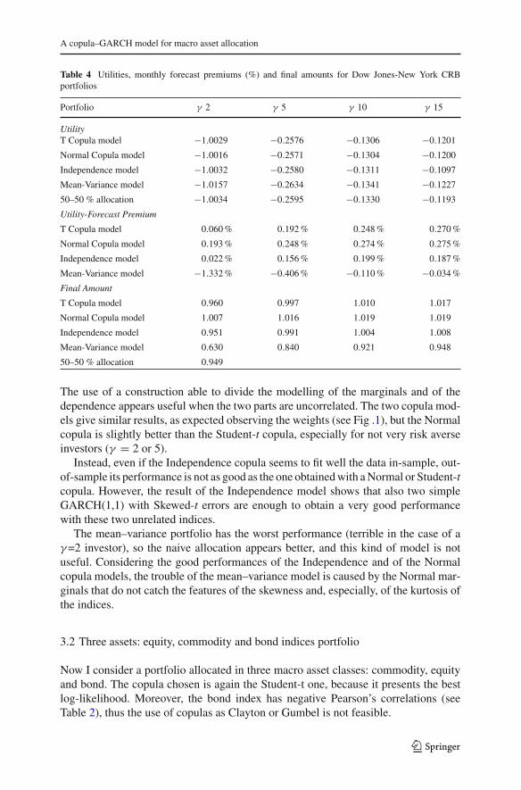
I consider two characteristics: the utility of the allocation and the amount of moneyobtained at the end of the entire out-of-sample period (all 36 months). The most impor-tant value is the utility, indeed it contains all the features of the obtained returns, thus themean return (and therefore the total return) is already included in this value. However,the mean return is the most important feature of the utility, especially for a low riskaverse person, so Table 4 presents both the utility and the final amount obtained. Theutility is calculated using the CRRA function and the monthly out-of-sample obtainedreturns. I report not only the value of the utility, but also the forecast premium abovethe 50–50 % portfolio (calculated using formula 3) to give an economic meaning tothe utility differences; obviously, the forecast premium is negative if the model givesa utility worse than the 50–50 % allocation.

By observing Table 4, it is evident that the copula models are the best at all γ levelsfor the macro asset allocation of this portfolio composed by equity and commodity.

circle: gamma 2square: gamma 5triangle: gamma 10

month0 5 10 15 20 25 30 35

wei

ght

0.0

0

.5

1.

0

1.

5

Fig. 2 Weights of Dow Jones for Student-t copula model with different γ values: 2, 5 and 10

123


Table 4 Utilities, monthly forecast premiums (%) and final amounts for Dow Jones-New York CRBportfolios

Portfolio γ 2 γ 5 γ 10 γ 15

UtilityT Copula model −1.0029 −0.2576 −0.1306 −0.1201

Normal Copula model −1.0016 −0.2571 −0.1304 −0.1200

Independence model −1.0032 −0.2580 −0.1311 −0.1097

Mean-Variance model −1.0157 −0.2634 −0.1341 −0.1227

50–50 % allocation −1.0034 −0.2595 −0.1330 −0.1193

Utility-Forecast Premium

T Copula model 0.060 % 0.192 % 0.248 % 0.270 %

Normal Copula model 0.193 % 0.248 % 0.274 % 0.275 %

Independence model 0.022 % 0.156 % 0.199 % 0.187 %

Mean-Variance model −1.332 % −0.406 % −0.110 % −0.034 %

Final Amount

T Copula model 0.960 0.997 1.010 1.017

Normal Copula model 1.007 1.016 1.019 1.019

Independence model 0.951 0.991 1.004 1.008

Mean-Variance model 0.630 0.840 0.921 0.948

50–50 % allocation 0.949

The use of a construction able to divide the modelling of the marginals and of thedependence appears useful when the two parts are uncorrelated. The two copula mod-els give similar results, as expected observing the weights (see Fig .1), but the Normalcopula is slightly better than the Student-t copula, especially for not very risk averseinvestors (γ = 2 or 5).

Instead, even if the Independence copula seems to fit well the data in-sample, out-of-sample its performance is not as good as the one obtained with a Normal or Student-tcopula. However, the result of the Independence model shows that also two simpleGARCH(1,1) with Skewed-t errors are enough to obtain a very good performancewith these two unrelated indices.

The mean–variance portfolio has the worst performance (terrible in the case of aγ =2 investor), so the naive allocation appears better, and this kind of model is notuseful. Considering the good performances of the Independence and of the Normalcopula models, the trouble of the mean–variance model is caused by the Normal mar-ginals that do not catch the features of the skewness and, especially, of the kurtosis ofthe indices.

3.2 Three assets: equity, commodity and bond indices portfolio

Now I consider a portfolio allocated in three macro asset classes: commodity, equityand bond. The copula chosen is again the Student-t one, because it presents the bestlog-likelihood. Moreover, the bond index has negative Pearson’s correlations (seeTable 2), thus the use of copulas as Clayton or Gumbel is not feasible.

123

L. Riccetti

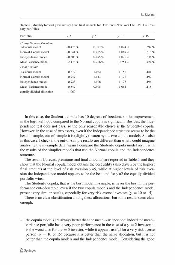
Table 5 Monthly forecast premiums (%) and final amounts for Dow Jones-New York CRB-ML US Trea-sury portfolios


Utility-Forecast PremiumT-Copula model −0.476 % 0.397 % 1.024 % 1.592 %

Normal-Copula model −0.241 % 0.485 % 1.067 % 1.619 %

Independence model −0.308 % 0.475 % 1.076 % 1.636 %

Mean-Variance model −2.178 % −0.206 % 0.751 % 1.424 %

Final Amount

T-Copula model 0.879 1.082 1.156 1.181

Normal-Copula model 0.947 1.113 1.172 1.192



equally divided allocation 1.060

In this case, the Student-t copula has 10 degrees of freedom, so the improvementin the log-likelihood compared to the Normal copula is significant. Besides, the inde-pendence test does not pass, so the only reasonable choice is the Student-t copula.However, in the case of two assets, even if the Independence structure seems to be thebest in-sample, out-of-sample it is (slightly) beaten by the two copula models. So, alsoin this case, I check if the out-of-sample results are different than what I could imagineanalysing the in-sample data: again I compare the Student-t copula model result withthe results of the simplier models that use the Normal copula and the Independencestructure.

The results (forecast premiums and final amounts) are reported in Table 5, and theyshow that the Normal copula model obtains the best utility (also driven by the highestfinal amount) at the level of risk aversion γ =5, while at higher levels of risk aver-sion the Independence model appears to be the best and for γ =2 the equally dividedportfolio wins.

The Student-t copula, that is the best model in-sample, is never the best in the per-formance out-of-sample, even if the two copula models and the Independence modelpresent very similar results, especially for very risk averse investors (γ = 10 or 15).

There is no clear classification among these allocations, but some results seem clearenough:

– the copula models are always better than the mean–variance one; indeed the mean–variance portfolio has a very poor performance in the case of a γ = 2 investor, itis the worst also for a γ = 5 investor, while it appears useful for a very risk averseperson (γ = 10 or 15) because it is better than the naive allocation, but it is notbetter than the copula models and the Independence model. Considering the good

123


performance of the Independence model and of the Normal copula, the improve-ment is due to the importance of the Skewed-t marginals.5;

– the use of a construction able to divide the modelling of the marginals and of thedependence, appears useful;

– for the macro asset allocation of a portfolio composed by equity, commodity andbond parts, which are all almost unrelated, the use of a copula model can be useful,but the use of univariate GARCH(1,1) with Skewed-t errors obtains good resultsalso. Thus, modelling the dependence structure in a complex way could be a wasteof energy and time;

– a good in-sample fit does not assure a good out-of-sample result.

3.3 Four assets: equity, commodity, bond and exchange rate portfolio

In this subsection, the portfolio is allocated on four macro asset classes: commodity,equity, bond and exchange rate. The comparison is done, as usual, with the equi-divided portfolio as benchmark (25%–25%–25%–25%). The Student-t copula has thebest log-likelihood in this case too. However, this copula does not pass the GOF test,so I try also a Canonical Vine copula. Indeed, in Riccetti (2010) the Canonical Vinecopula improves the performance compared to the Student-t copula, in a four assetsportfolio with one uncorrelated index. All the bivariate copulas that compose the Vinecopula are Student-t, indeed some assets have negative correlations, so the use ofClayton or Gumbel copulas is not feasible. Moreover, the Student-t copulas give thebest fit according to several authors, such as Aas et al. (2007).

Now, the problem is the choice of the order of the building blocks. The first indexis the one that has a bivariate copula with each of the other indices; the second index,conditional to the first index, has two bivariate copulas with the two remaining indi-ces; and finally there are the two last indices with the copula between them. I try fourorders:

(1) order 1: bond index, exchange rate (then equity index and commodity index).The first tree is the one that presents the highest values of the tail dependences(calculated using the Student-t copula estimates) reported in Table 6, and so on;this is the method suggested by Berg and Aas (2007);

(2) order 2: exchange rate, bond index (equity index and commodity index). Thefirst tree is the one that presents the highest absolute values of the Kendall’s Tau,reported in Table 9 (Appendix A), and so on;

(3) order 3: commodity index, equity index (exchange rate and bond index). Thisis the opposite of the first order, beginning with the index with the lowest taildependence;

(4) order 4: equity index, commodity index (exchange rate and bond index). Thefirst tree has all negative relations (as Kendall’s Tau, see Table 9, or Pearson’s

5 This conclusion is different from Patton (2004), indeed Patton finds that the dependence structure is morerelevant than the marginal one. However, Patton uses two stock indices and the U.S.Treasury bill interestrate, and the two stock indices have a high correlation.

123

L. Riccetti

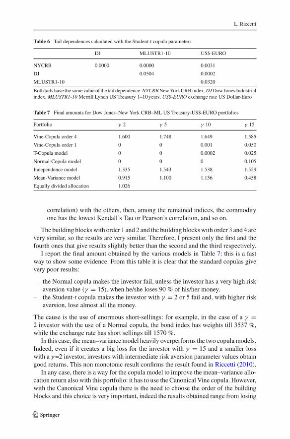
Table 6 Tail dependences calculated with the Student-t copula parameters

DJ MLUSTR1-10 US$-EURO

NYCRB 0.0000 0.0000 0.0031

DJ 0.0504 0.0002

MLUSTR1-10 0.0320

Both tails have the same value of the tail dependence. NYCRB New York CRB index, DJ Dow Jones Industrialindex, MLUSTR1-10 Merrill Lynch US Treasury 1–10 years, US$-EURO exchange rate US Dollar-Euro

Table 7 Final amounts for Dow Jones–New York CRB–ML US Treasury-US$-EURO portfolios


Vine-Copula order 4 1.600 1.748 1.649 1.585

Vine-Copula order 1 0 0 0.001 0.050

T-Copula model 0 0 0.0002 0.025

Normal-Copula model 0 0 0 0.105



Equally divided allocation 1.026

correlation) with the others, then, among the remained indices, the commodityone has the lowest Kendall’s Tau or Pearson’s correlation, and so on.

The building blocks with order 1 and 2 and the building blocks with order 3 and 4 arevery similar, so the results are very similar. Therefore, I present only the first and thefourth ones that give results slightly better than the second and the third respectively.

I report the final amount obtained by the various models in Table 7: this is a fastway to show some evidence. From this table it is clear that the standard copulas givevery poor results:

– the Normal copula makes the investor fail, unless the investor has a very high riskaversion value (γ = 15), when he/she loses 90 % of his/her money.

– the Student-t copula makes the investor with γ = 2 or 5 fail and, with higher riskaversion, lose almost all the money.

The cause is the use of enormous short-sellings: for example, in the case of a γ =2 investor with the use of a Normal copula, the bond index has weights till 3537 %,while the exchange rate has short sellings till 1570 %.

In this case, the mean–variance model heavily overperforms the two copula models.Indeed, even if it creates a big loss for the investor with γ = 15 and a smaller losswith a γ =2 investor, investors with intermediate risk aversion parameter values obtaingood returns. This non monotonic result confirms the result found in Riccetti (2010).

In any case, there is a way for the copula model to improve the mean–variance allo-cation return also with this portfolio: it has to use the Canonical Vine copula. However,with the Canonical Vine copula there is the need to choose the order of the buildingblocks and this choice is very important, indeed the results obtained range from losing

123


all the money to having a return of 75 % in 3 years. Following the suggestions of Bergand Aas (2007), that is using as the first two factors the indices with the highest taildependence or Kendall’s Tau, the results are disastrous. Moreover, these values canchange from the in-sample to the out-of-sample data, as shown by the Kendall’s Taureported in Tables 9 and 10 (Appendix A).

The Independence model gives very good returns at all levels of risk aversion, andit is beaten only by the Vine copula models with building blocks that follow order 3 or4. However, this model appears to be a very safe (you cannot be wrong in the choiceof the building blocks order) and simple way to obtain excellent returns.

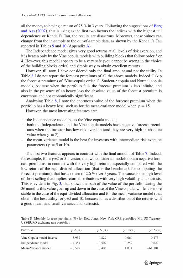
However, till now, I have considered only the final amount and not the utility. InTable 8 I do not report the forecast premiums of all the above models. Indeed, I skipthe forecast premiums of ‘Vine-copula order 1’, Student-t copula and Normal copulamodels, because when the portfolio fails the forecast premium is less infinite, andalso in the presence of an heavy loss the absolute value of the forecast premium isenormous and not economically significant.

Analysing Table 8, I note the enormous value of the forecast premium when theportfolio has a heavy loss, such as for the mean-variance model when γ = 15.

However, the most interesting features are:

– the Independence model beats the Vine copula model;– both the Independence and the Vine copula models have negative forecast premi-

ums when the investor has low risk aversion (and they are very high in absolutevalue when γ = 2);

– the mean-variance model is the best for investors with intermediate risk aversionparameters (γ = 5 or 10).

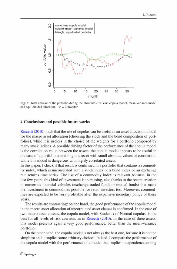
The first two features appears in contrast with the final amount of Table 7. Indeed,for example, for a γ =2 or 5 investor, the two considered models obtain negative fore-cast premiums, in contrast with the very high returns, especially compared with thelow return of the equi-divided allocation (that is the benchmark for computing theforecast premium), that has a return of 2,6 % over 3 years. The cause is the high levelof short-selling that implies return distributions with very high volatility and kurtosis.This is evident in Fig. 3, that shows the path of the value of the portfolio during the36 months: this value goes up and down in the case of the Vine copula, while it is morestable in the case of the equi-divided allocation and for the mean-variance model (thatobtains the best utility for γ =5 and 10, because it has a distribution of the returns witha good mean, and small variance and kurtosis).

Table 8 Monthly forecast premiums (%) for Dow Jones–New York CRB portfolios–ML US Treasury-US$/EURO exchange rate portfolios

Portfolio γ 2 (%) γ 5 (%) γ 10 (%) γ 15 (%)

Vine Copula model-inverse −5.957 −0.829 0.060 0.473

Indipendence model −4.354 −0.509 0.259 0.629

Mean-Variance model −0.599 0.405 1.014 −61.101

123

L. Riccetti

port

folio

val

ue0.

0

0.5

1.0

1

.5

2.

0 circle: vine copula modelsquare: mean−variance modeltriangle: equidivided portfolio

month

0 5 10 15 20 25 30 35

Fig. 3 Total amount of the portfolio during the 36 months for Vine copula model, mean-variance modeland equi-divided allocation—γ = 2 investor

4 Conclusions and possible future works

Riccetti (2010) finds that the use of copulas can be useful in an asset allocation modelfor the macro asset allocation (choosing the stock and the bond composition of port-folios), while it is useless in the choice of the weights for a portfolio composed bymany stock indices. A possible driving factor of the performance of the copula modelis the correlation value between the assets: the copula model appears to be useful inthe case of a portfolio containing one asset with small absolute values of correlation,while this model is dangerous with highly correlated assets.In this paper, I check if that result is confirmed in a portfolio that contains a commod-ity index, which is uncorrelated with a stock index or a bond index or an exchangerate returns time series. The use of a commodity index is relevant because, in thelast few years, this kind of investment is increasing, also thanks to the recent creationof numerous financial vehicles (exchange traded funds or mutual funds) that makethe investment in commodities possible for retail investors too. Moreover, commod-ities are expected to be very profitable after the expansive monetary policy of theseyears.

The results are contrasting: on one hand, the good performance of the copula modelin the macro asset allocation of uncorrelated asset classes is confirmed. In the case oftwo macro asset classes, the copula model, with Student-t of Normal copulas, is thebest for all levels of risk aversion, as in Riccetti (2010). In the case of three assets,this model presents again a very good performance, better than the mean-varianceportfolio.

On the other hand, the copula model is not always the best one, for sure it is not thesimpliest and it implies some arbitrary choices. Indeed, I compare the performance ofthe copula model with the performance of a model that implies independence among

123


the univariate series of residuals, because it is a reasonable way to model almostuncorrelated asset classes. This kind of model is faster and simpler, because it needsonly the univariate GARCH, with a suitable distribution of the error terms, such asthe Skewed-t one. The comparison shows that the Independence model produces out-of-sample results more or less similar to those obtained by the copula model, but witha simpler method. Moreover, the improvement of the Independence model over themean-variance one is high and it means that, with these indices, it is more importantto catch the features of the return distribution of the single asset classes, than to catchthe joint behaviour of the multivariate distribution of the returns. Perhaps this featureis tied to the fact that the macro asset allocation is done on almost unrelated classes.However, as shown in Riccetti (2010), the copula model is useless also for portfoliosinvolving very related assets, as all stock indices. Thus, the copula model appearsnot useful at all, with the exception of portfolios containing one uncorrelated asset.Indeed, the copula model obtains the best (among the tried models) out-of-sampleperformance, when the portfolio is invested in:

– two uncorrelated assets (or asset classes), such as commodities and stocks, asshown in this paper;

– two or more correlated indices and one less correlated one, as shown in Riccetti(2010) or Patton (2004) with portfolios invested in two or three stock indices andone safer index.

However, there are a lot of possible works in this field to confirm or deny the gen-eral conclusions enunciated (if general conclusions, which can be applied in differentsituations, really exist):

– there could be situations in which the copula model is the best, using other indi-ces and/or using other periods and/or using other allocation horizons and/or usingother frequency of returns and/or using a multiperiodal framework and/or usingother utility functions and/or considering the uncertainty related to the estimationof the parameters and/or using the short-selling constraint;

– there could be different models of the marginal distributions of returns (for themean, the variance…) and for the copulas (such as the Skewed-t copula used inSun et al. (2009) and Rachev et al. (2011)), and/or model extensions, for examplewith dynamic conditional parameters (again for mean forecast or for skewness andkurtosis of the marginal distribution of residuals or for the copula parameters, seealso Appendix B).

Moreover, in this paper, it seems that the complex models tend to overfit the datain-sample, but they are often too specific to obtain a good performance out-of-sam-ple. Further research could analyse the use of even more complex copula models,to understand if they improve the out-of-sample forecasting: I cannot exclude thatthe relationship between complexity and the out-of-sample performance could be Ushaped, with an initial decrease and a following increase with very complex models(for example using a dynamic copula).

A possible case of a U shaped relation between complexity and performance foundin this paper is that, when the number of assets increases, the standard copula modelshows increasing problems, but the use of Vine copulas can reduce these problems

123

L. Riccetti

(even if they are still present). However, very complex structures can imply severalother problems. For instance, a Vine copula gives problems in the choice of the singlebivariate copulas and problems in the choice of the order of the indices in the buildingblocks; as shown, these choices can change the results dramatically and the betterin-sample choice can no longer be good out-of-sample. Indeed, a clear feature thatemerges from this paper is that the good in-sample fit does not assure a good out-of-sample result. Instead, methods that do not use strong assumptions to improve thein-sample fit, like the Independence one, often seem more robust than more complexmodels, as the copula ones.

In conclusion, the use of a simple GARCH(1,1) with Skewed-t errors for each assetclass seems to be enough to obtain a good performance in the macro asset allocation ofa portfolio that uses commodities. Indeed, even if I find that the copula model appearsuseful and better than the mean-variance one, it is often worse than a set of indepen-dent univariate GARCH(1,1) models, probably because commodities have returns thatare almost unrelated to the returns of the other macro asset classes (stock, bond andexchange rate).

Acknowledgements I am very grateful to Dean Fantazzini, Riccardo Lucchetti, Giulio Palomba and theparticipants of the ‘Third Rimini Finance Workshop’ (Rimini-Italy, 30 May 2011, organized by ‘The RiminiCentre for Economic Analysis—RCEA’) for helpful comments and suggestions.

A Appendix: multivariate dependence

Most of the research on copulas is limited to the bivariate case. The set of higher-dimen-sional copulae is limited, and the copulas that can be generalized to the multivariatecase, often imply the strong restriction that the dependence is the same across all pairsof variables. In recent years, some authors have tried to construct more flexible mul-tivariate copulas by modelling multivariate dependence with a cascade of bivariatecopulas. Some extensions are the nested Archimedean constructions discussed in Joe(1997); Embrechts et al. (2003); Whelan (2004) and McNeil (2007). These methodsuse up to d-1 bivariate Archimedean copulas. However, they have some limits: theyonly use Archimedean copulas, they do not model all possible mutual dependenciesamong the d variates and they have to satisfy necessary conditions to lead to validmultivariate copulas.

I therefore use another kind of construction, denoted pair-copula constructions(PCC), first proposed by Joe (1997) and either discussed or applied by Bedford andCooke (2001, 2002); Kurowicka and Cooke (2006); Aas et al. (2007); Berg and Aas(2007); Heinen and Valdesogo (2008) and Haff et al. (2009). The PCC is more flexible,indeed it allows for the free specification of d(d–1)/2 copulas and uses all kinds ofbivariate copulas; furthermore, it does not have parameter constraints.

The most frequently used type of PCC is the regular vine type and, in particular, twospecial cases of regular vine: the Canonical Vines and the D-vines. I use the Canoni-cal Vine copula that decomposes the joint probability density function of n variablesy1, . . . , yn through iterative conditioning, as follows:

123


f (y1, . . . , yn) = f (y1) · f (y2|y1) · f (y3|y1, y2) . . . f (yn|y1, . . . , yn−1) (4)

Each factor in this product can be further decomposed using conditional copulas, forexample:

f (y2|y1) = c12(F(y1), F(y2)) · f (y2) (5)

f (y3|y1, y2) = c23|1(F(y2|y1), F(y3|y1)) · f (y3|y1) (6)

Finally, combining all the expressions I obtain the joint density, that is the productof marginals densities and bivariate conditional copulas densities. For instance, for athree dimensional case, this is the joint density function:

f (y1, y2, y3) = c23|1(F(y2|y1), F(y3|y1))c12(F(y1), F(y2))c13(F(y1), F(y3)) f (y1) f (y2) f (y3)

(7)

The parameters are estimated by maximum likelihood with a recursive approach, asexplained in Aas et al. (2007).

The PCC approach has some shortcomings. One is that there are almost unlim-ited ways to combine each building block, so the problem of not having enoughmultivariate copulas is reversed. Another problem is that the estimation processhas a number of steps that increases rapidly with the dimension and the complex-ity of the copula, so it becomes time consuming. Moreover, as analysed by Haffet al. (2009), the exact decomposition is based on pair-copula of the followingform:

C23|1(F(y2|y1), F(y3|y1); y1) (8)

but, for inference to be fast, flexible and robust, I assume that these pair-copulas areindependent of the conditioning variables, except through the conditional distribu-tion:

C23|1(F(y2|y1), F(y3|y1)) (9)

However, in Haff et al. (2009), the authors show that, even if the pair-cop-ula is dependent on the conditioning variable so that the simplyfied decom-position is wrong, this is a good approximation of the general decomposition.Then, in this study, I also use Canonical Vine copulas for multivariate alloca-tions.

B Appendix: why a dynamic copula could be useful

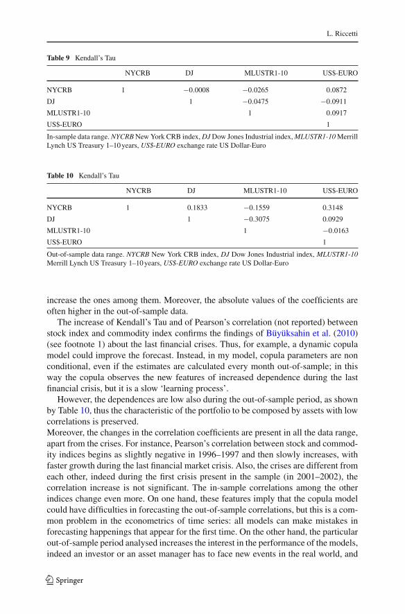
Pearson’s correlation matrix and Kendall’s Tau matrix change over time. A significantchange is present between the in-sample and the out-of-sample data range (whichcorresponds to the last financial crises), as shown in Tables 9 and 10: the bond indexdecreases its Kendall’s Tau values with the other indices, while the other three indices

123

L. Riccetti



NYCRB 1 −0.0008 −0.0265 0.0872

DJ 1 −0.0475 −0.0911

MLUSTR1-10 1 0.0917

US$-EURO 1

In-sample data range. NYCRB New York CRB index, DJ Dow Jones Industrial index, MLUSTR1-10 MerrillLynch US Treasury 1–10 years, US$-EURO exchange rate US Dollar-Euro



NYCRB 1 0.1833 −0.1559 0.3148

DJ 1 −0.3075 0.0929

MLUSTR1-10 1 −0.0163

US$-EURO 1

Out-of-sample data range. NYCRB New York CRB index, DJ Dow Jones Industrial index, MLUSTR1-10Merrill Lynch US Treasury 1–10 years, US$-EURO exchange rate US Dollar-Euro

increase the ones among them. Moreover, the absolute values of the coefficients areoften higher in the out-of-sample data.

The increase of Kendall’s Tau and of Pearson’s correlation (not reported) betweenstock index and commodity index confirms the findings of Büyüksahin et al. (2010)(see footnote 1) about the last financial crises. Thus, for example, a dynamic copulamodel could improve the forecast. Instead, in my model, copula parameters are nonconditional, even if the estimates are calculated every month out-of-sample; in thisway the copula observes the new features of increased dependence during the lastfinancial crisis, but it is a slow ‘learning process’.

However, the dependences are low also during the out-of-sample period, as shownby Table 10, thus the characteristic of the portfolio to be composed by assets with lowcorrelations is preserved.Moreover, the changes in the correlation coefficients are present in all the data range,apart from the crises. For instance, Pearson’s correlation between stock and commod-ity indices begins as slightly negative in 1996–1997 and then slowly increases, withfaster growth during the last financial market crisis. Also, the crises are different fromeach other, indeed during the first crisis present in the sample (in 2001–2002), thecorrelation increase is not significant. The in-sample correlations among the otherindices change even more. On one hand, these features imply that the copula modelcould have difficulties in forecasting the out-of-sample correlations, but this is a com-mon problem in the econometrics of time series: all models can make mistakes inforecasting happenings that appear for the first time. On the other hand, the particularout-of-sample period analysed increases the interest in the performance of the models,indeed an investor or an asset manager has to face new events in the real world, and

123


the possibility to use a model that is efficient in facing also extreme events is a veryimportant characteristic.

In conclusion, as already said in Sect. 4, it could be interesting to develop furtherresearch to enrich the model, to understand if a more complex one can improve theout-of-sample forecasting.

References

Aas K, Czado C, Frigessi A, Bakken H (2007) Pair-copula constructions of multiple dependence. InsurMath Econ 4(2):182–188

Abanomey W, Mathur I (1999) The hedging benefits of commodity futures in international portfolio diver-sification. J Altern Invest 2(3):51–62

Amenc N, Martellini L, Ziemann V (2009) Inflation-hedging properties of real assets and implications forasset–liability management decisions. J Portfolio Manag 35(4):94–110

Anderson T (2008) Real assets inflation protection solutions with exchange-traded products. ETFs Index1:14–24

Ang A, Bekaert G (2002) International asset allocation with regime shifts. Rev Financ Stud 15(4):1137–1187

Arditti F (1967) Risk and the required return on equity. J Finance 22:19–36Bedford T, Cooke R (2001) Probability density decomposition for conditionally dependent random vari-

ables modeled by vines. Ann Math Artif Intell 32:245–268Bedford T, Cooke R (2002) Vines: a new graphical model for dependent random variables. Ann Stat

30:1031–1068Berg D (2008) Copula goodness-of-fit testing: an overview and power comparison, working paper, Univer-

sity of Oslo and The Norwegian Computing CenterBerg D, Aas K (2007) Model for construction of multivariate dependence, technical report, working paper,

Norwegian Computing CenterBodie Z (1983) Commodity futures as a hedge against inflation. J Portfolio Manag 9:12–17Bucciol A, Miniaci R (2008) Household portfolios and implicit risk aversion, working paperBüyüksahin B, Haigh M, Robe M (2010) Commodities and equities: ever a ‘market of one’?. J Altern Invest

12(3):76–95Chong J, Miffre J (2010) Conditional correlation and volatility in commodity futures and traditional asset

markets. J Altern Invest 12(3):61–75Conover C, Jensen G, Johnson R, Mercer J (2010) Is now the time to add commodities to your portfolio?.

Financ Anal J 61(1):57–69Dempster N, Artigas J (2010) Gold: inflation hedge and long-term strategic asset. J Wealth Manag 13(2):

69–75Dittmar R (2002) Nonlinear pricing kernels, kurtosis preferences, and evidence from the cross section of

equity returns. J Finance 57:369–403Embrechts P, Lindskog F, McNeil A (2003) Modelling dependence with copulas and applications to

risk management. In: Rachev ST (ed) Handbook of heavy tailed distributions in finance. Elsevier,Amsterdam

Embrechts P, Frey R, McNeil A (2005) Quantitative risk management: concepts, techniques and tools.Princeton University Press, Princeton

Froot K (1995) Hedging portfolios with real assets. J Portfolio Manag 18:60–77Genest C, Rémillard B (2004) Tests of independence and randomness based on the empirical copula process.

Test 13:335–369Genest C, Rémillard B (2008) Validity of the parametric bootstrap for goodness-of-fit testing in semipara-

metric models. Ann Inst H Poincaré Probab Stat 44(6):1096–1127Genest C, Rémillard B, Beaudoin D (2009) Goodness-of-fit tests for copulas: a review and a power study.

Insur Math Econ 44:199–213Gorton G, Rouwenhorst K (2006) Facts and fantasies about commodity futures. Financ Anal J 62:47–68Haff I, Aas K, Frigessi A (2009) On the simplified pair-copula construction: simply useful or too simplistic?,

working paper

123

L. Riccetti

Halpern P, Warsager R (1998) The performance of energy and non-energy based commodity investmentvehicles in periods of inflation. J Altern Invest 1(1):75–81

Harvey C, Siddique A (2000) Conditional skewness in asset pricing tests. J Finance 55(3):1263–1295Heinen A, Valdesogo A (2008) Asymmetric capm dependence for large dimensions: the canonical vine

autoregressive model, working paperIgnatieva K, Platen E (2010) Modelling co-movements and tail dependency in the international stock market

via copulae. Asia Pacific Financ Mark 17:261–302. doi:10.1007/s10690-010-9116-2Irwin S, Landa D (1987) Real estate, futures, and gold as portfolio assets. J Portfolio Manag 14:29–34Jensen G, Johnson R, Mercer J (2000) Efficient use of commodity futures in diversified portfolios. J Futur

Mark 20:489–506Jensen G, Johnson R, Mercer J (2002) Tactical asset allocation and commodity futures. J Portfolio Manag

28(4):100–111Joe H (1997) Multivariate models and dependence concepts. Chapman and Hall, LondonJondeau E, Rockinger M (2003) Conditional volatility, skewness, and kurtosis: existence, persistence and

comovements. J Econ Dyn Control (Elsevier) 27:1699–1737Jondeau E, Rockinger M (2006a) The Copula–GARCH model of conditional dependencies: an international

stock market application. J Int Money Finance (Elsevier) 25:827–853Jondeau E, Rockinger M (2006b) Optimal portfolio allocation under higher moments. Eur Financ Manag

12(1):29–55Kraus A, Litzenberger R (1976) Skewness preference and the valuation of risk assets. J Finance 31(4):

1085–1100Kurowicka D, Cooke R (2006) Uncertainty analysis with high dimensional dependence modelling. Wiley,

New YorkMandelbrot B (1963) The variation of certain speculative prices. J Bus 36:394–419Markowitz H (1952) Portfolio selection. J Finance 7(1):77–91Mazzilli P, Maister D (2006) Exchange-traded funds six ETFs provide exposure to commodity markets.

ETFs Index 1:26–34McNeil A (2007) Sampling nested archimedean copulas. J Stat Comput Simul 4:339–352Morana C (2009) Realized betas and the cross-section of expected returns. Appl Financ Econ 19:1371–1381Patton (2004) On the out-of-sample importance of skewness and asymmetric dependence for asset

allocation. J Financ Econom 2(1):130–168Rachev S, Kim Y, Bianchi M, Fabozzi F (2011) Financial models with Lévy processes and volatility

clustering. Wiley, New JerseyRiccetti L (2010) The use of copulas in asset allocation: when and how a copula model can be useful? LAP

Lambert, SaarbrückenScott R, Horvath P (1980) On the direction of preference for moments of higher order than the variance. J

Finance XXXV(4):915–919Simkowitz M, Beedles W (1978) Diversification in a three moment world. J Financ Quant Anal 13:927–941Sklar A (1959) Fonctions de répartition à n dimensions et leurs marges. Inst Statist Univ Paris 8:229–231Sun W, Rachev S, Stoyanov S, Fabozzi F (2008) Multivariate skewed student’s t copula in the analysis of

nonlinear and asymmetric dependence in the German equity market. Stud Nonlinear Dyn Econom12(2):article 3

Sun W, Rachev S, Fabozzi F, Kalev P (2009) A new approach to modeling co-movement of internationalequity markets: evidence of unconditional copula-based simulation of tail dependence. Empir Econ36(1):201–229. doi:10.1007/s00181-008-0192-3

Whelan N (2004) Sampling from archimedean copulas. Quant Finance 4:339–352

123

http://dx.doi.org/10.1007/s10690-010-9116-2

http://dx.doi.org/10.1007/s00181-008-0192-3

Documents

A copula–GARCH model for macro asset allocation of a portfolio with commodities