Embed Size (px)
Citation preview

A Cosmological Fireball with Thirty-PercentGamma-Ray Radiative E�ciencyLiang Li ( [email protected] )
ICRANetYu Wang
Sapienza University of RomeFelix Ryde
KTH Royal Institute of TechnologyAsaf Pe'er
Bar-Ilan UniversityBing Zhang
University of Nevada, Las Vegas https://orcid.org/0000-0002-9725-2524Sylvain Guiriec
The George Washington UniversityAlberto Castro-Tirado
IAA-CSICDavid Alexander Kann
Instituto de Astrofısica de Andalucıa https://orcid.org/0000-0003-2902-3583Magnus Axelsson
Royal Institute of Technology (KTH)Kim Page
University of Leicester https://orcid.org/0000-0001-5624-2613Peter Veres
University of Alabama HuntsvilleNarayana Perumpalli Bhat
University of Alabama Huntsville
Letter
Keywords: gamma-ray bursts (GRBs), radiative e�ciency
Posted Date: February 17th, 2021
DOI: https://doi.org/10.21203/rs.3.rs-231408/v1

License: This work is licensed under a Creative Commons Attribution 4.0 International License. Read Full License

A Cosmological Fireball with Thirty-Percent Gamma-Ray
Radiative Efficiency
Liang Li1,2,3∗, Yu Wang1,2,3∗, Felix Ryde4, Asaf Pe’er5, Bing Zhang6∗, Sylvain Guiriec7,8, Alberto
J. Castro-Tirado9,10, D. Alexander Kann9, Magnus Axelsson11, Kim Page12, Peter Veres13, P. N.
Bhat13,14
1ICRANet, Piazza della Repubblica 10, 65122 Pescara, Italy2INAF – Osservatorio Astronomico d’Abruzzo, Via M. Maggini snc, I-64100, Teramo, Italy3Dip. di Fisica and ICRA, Sapienza Universita di Roma, Piazzale Aldo Moro 5, I-00185 Rome, Italy4Department of Physics, KTH Royal Institute of Technology, and the Oskar Klein Centre for Cosmoparticle
Physics, 10691 Stockholm, Sweden5Department of Physics, Bar-Ilan University, Ramat-Gan 52900, Israel6Department of Physics and Astronomy, University of Nevada, Las Vegas, NV 89154, USA7Department of Physics, The George Washington University, 725 21st Street NW, Washington, DC 20052,
USA8NASA Goddard Space Flight Center, Greenbelt, MD 20771, USA9Instituto de Astrofısica de Andalucıa (IAA-CSIC), PO Box 03004, Granada, Spain10Departamento de Ingenierıa de Sistemas y Automatica, Escuela de Ingenierıas, Universidad de Malaga,
Malaga, Spain11Department of Astronomy, Stockholm University, SE-106 91 Stockholm, Sweden12School of Physics and Astronomy, University of Leicester, University Road, Leicester LE1 7RH, UK13Center for Space Plasma and Aeronomic Research, University of Alabama in Huntsville,
Huntsville,AL,USA14Space Science Department,University of Alabama in Huntsville, Huntsville, AL,USA∗E-mail: [email protected]; [email protected]; [email protected]
Gamma-ray bursts (GRBs) are the most powerful explosions in the universe. The compo-
sition of the jets is, however, subject to debate1, 2. Whereas the traditional model invokes a
relativistic matter-dominated fireball with a bright photosphere emission component3, the
lack of the detection of such a component in some GRBs4 has led to the conclusion that GRB
jets may be Poynting-flux-dominated5. Furthermore, how efficiently the jet converts its en-
ergy to radiation is poorly constrained. A definitive diagnosis of the GRB jet composition
and measurement of GRB radiative efficiency requires high-quality prompt emission and
afterglow data, which has not been possible with the sparse observations in the past. Here
we report a comprehensive temporal and spectral analysis of the TeV-emitting bright GRB
190114C. Its fluence is one of the highest of all GRBs detected so far, which allows us to
perform a high-significance study on the prompt emission spectral properties and their vari-
ations down to a very short timescale of about 0.1 s. We identify a clear thermal component
during the first two prompt emission episodes, which is fully consistent with the prediction of
the fireball photosphere model. The third episode of the prompt emission is consistent with
synchrotron radiation from the deceleration of the fireball. This allows us to directly dis-
1

sect the fireball energy budget in a parameter-independent manner6 and robustly measure
a nearly 30% radiative efficiency for this GRB. The afterglow microphysics parameters can
be also well constrained from the data. GRB 190114C, therefore, exhibits the evolution of a
textbook-version relativistic fireball, suggesting that fireballs can indeed power at least some
GRBs with high efficiency.
On 14 January 2019 at 20:57:02.63 Universal Time (UT) (hereafter T0), an ultra-bright
burst, GRB 190114C, was first triggered on by the Gamma-ray Burst Monitor (GBM) onboard
the Fermi Gamma-ray Space Telescope7 and the Neil Gehrels Swift Observatory’s (Swift here-
after) Burst Alert Telescope (BAT)8. Soon after, the Large Area Telescope (LAT) onboard Fermi,
Konus-Wind, INTEGRAL/SPI-ACS, AGILE/MCAL, and the Insight-HXMT/HE were also trig-
gered. Long-lasting and multi-wavelength afterglow observations were carried out by Swift in
the X-ray and optical bands, and by several ground-based optical and radio telescopes (such as
GROND9, GTC10, VLA11, MeerKAT12).
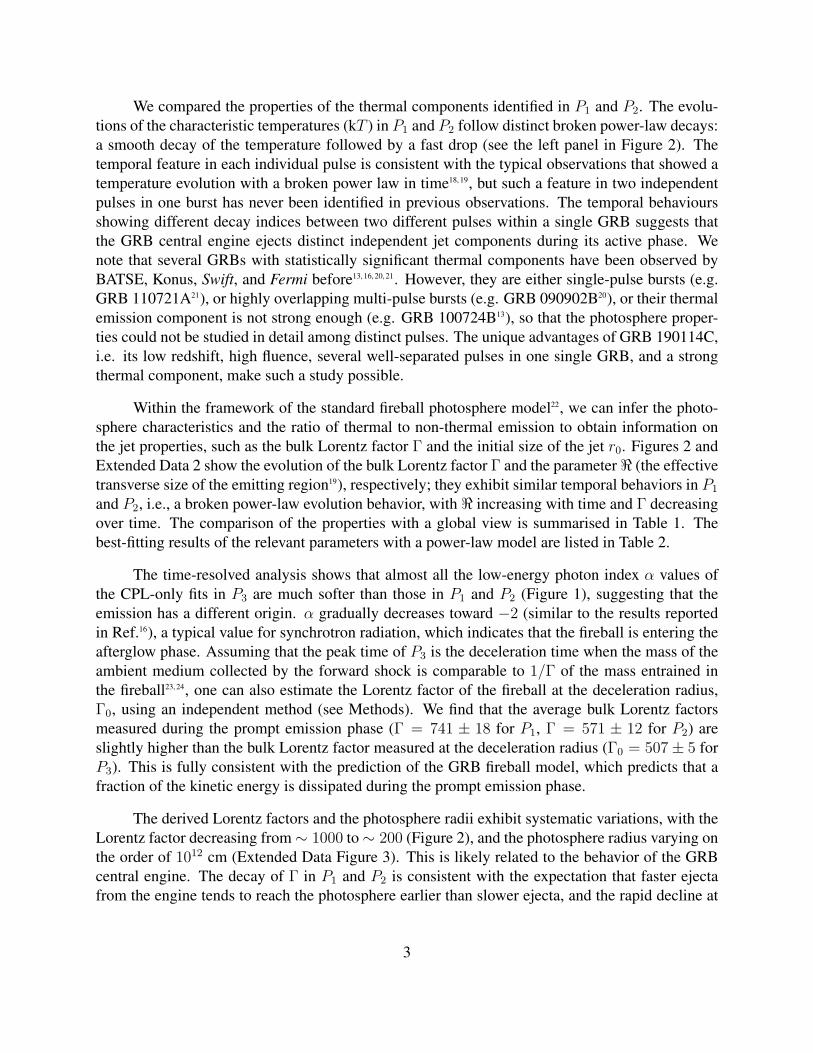
The prompt emission lightcurve (Figure 1) consists of three distinct emission episodes. The
first emission episode (i.e., P1) starts at ∼ T0 and lasts for ∼ 2.35 s, the second emission episode
(i.e., P2) exhibits multiple peaks and lasts from ∼ T0+2.35 s to ∼ T0+15 s, and the significantly
fainter third emission episode (i.e., P3) extends from ∼ T0+15 s to ∼ T0+25 s. First, P1 and P2
exhibit a non-thermal and a sub-dominant thermal component as first discovered in Ref.13. The
thermal components in P1 and P2 evolve independently (Figure 2). Such a feature provides a
unique opportunity to study the jet composition and photosphere properties at distinctly different
epochs of central engine activities. Second, the non-thermal spectral shape in P3 is consistent
with a synchrotron-radiation origin from afterglow emission14, 15. The afterglow phase of this GRB
has the most complete observations in terms of spectral coverage, from radio all the way to TeV
gamma-rays. This provides another unique opportunity to study the GRB afterglow properties
within the framework of synchrotron and synchrotron self-Compton model.
We perform a time-resolved spectral analysis for the Fermi-GBM observations. Thanks to
its high fluence of (4.436±0.005)×10−4 erg cm−2 as the fifth highest fluence GRB ever observed
with Fermi-GBM, we were able to divide its T90 (measured as the time interval between when
5% and 95% of the total flux was recorded) duration (116 s) into 48 slices, with each time bin
containing enough photons to conduct a high-significance spectral analysis (see Methods). The
CPL+BB (CPL: Cutoff powerlaw, BB: Blackbody) model13, 16 gives a better fit in comparison with
the CPL model and other models (see Methods) from T0+0.55 s to T0+1.93 s in P1 (includes 8
slices, hereafter P th1 ) and from T0+2.45 s to T0+5.69 s in P2 (includes 16 slices, hereafter P th
2 )
based on the deviance information criterion (DIC). P th1 and P th
2 correspond to the peak flux of the
P1 and P2, respectively, which precisely correspond to the epochs when the power-law index αof the single CPL fits (see Methods) are beyond the limits of the synchrotron line of death17, i.e.
α > −2/3. This is an indication of the existence of a thermal component as also reported in Ref.16.
An example of an νFν spectrum for one time slice (4.95 s–5.45 s) with the CPL+BB model giving
the best fit is displayed in Figure 3. In this example, a thermal component is superimposed on the
CPL component that is presumably of a synchrotron origin.
2
We compared the properties of the thermal components identified in P1 and P2. The evolu-
tions of the characteristic temperatures (kT ) in P1 and P2 follow distinct broken power-law decays:
a smooth decay of the temperature followed by a fast drop (see the left panel in Figure 2). The
temporal feature in each individual pulse is consistent with the typical observations that showed a
temperature evolution with a broken power law in time18, 19, but such a feature in two independent
pulses in one burst has never been identified in previous observations. The temporal behaviours
showing different decay indices between two different pulses within a single GRB suggests that
the GRB central engine ejects distinct independent jet components during its active phase. We
note that several GRBs with statistically significant thermal components have been observed by
BATSE, Konus, Swift, and Fermi before13, 16, 20, 21. However, they are either single-pulse bursts (e.g.
GRB 110721A21), or highly overlapping multi-pulse bursts (e.g. GRB 090902B20), or their thermal
emission component is not strong enough (e.g. GRB 100724B13), so that the photosphere proper-
ties could not be studied in detail among distinct pulses. The unique advantages of GRB 190114C,
i.e. its low redshift, high fluence, several well-separated pulses in one single GRB, and a strong
thermal component, make such a study possible.
Within the framework of the standard fireball photosphere model22, we can infer the photo-
sphere characteristics and the ratio of thermal to non-thermal emission to obtain information on
the jet properties, such as the bulk Lorentz factor Γ and the initial size of the jet r0. Figures 2 and
Extended Data 2 show the evolution of the bulk Lorentz factor Γ and the parameter ℜ (the effective
transverse size of the emitting region19), respectively; they exhibit similar temporal behaviors in P1
and P2, i.e., a broken power-law evolution behavior, with ℜ increasing with time and Γ decreasing
over time. The comparison of the properties with a global view is summarised in Table 1. The
best-fitting results of the relevant parameters with a power-law model are listed in Table 2.
The time-resolved analysis shows that almost all the low-energy photon index α values of
the CPL-only fits in P3 are much softer than those in P1 and P2 (Figure 1), suggesting that the
emission has a different origin. α gradually decreases toward −2 (similar to the results reported
in Ref.16), a typical value for synchrotron radiation, which indicates that the fireball is entering the
afterglow phase. Assuming that the peak time of P3 is the deceleration time when the mass of the
ambient medium collected by the forward shock is comparable to 1/Γ of the mass entrained in
the fireball23, 24, one can also estimate the Lorentz factor of the fireball at the deceleration radius,
Γ0, using an independent method (see Methods). We find that the average bulk Lorentz factors
measured during the prompt emission phase (Γ = 741 ± 18 for P1, Γ = 571 ± 12 for P2) are
slightly higher than the bulk Lorentz factor measured at the deceleration radius (Γ0 = 507± 5 for
P3). This is fully consistent with the prediction of the GRB fireball model, which predicts that a
fraction of the kinetic energy is dissipated during the prompt emission phase.
The derived Lorentz factors and the photosphere radii exhibit systematic variations, with the
Lorentz factor decreasing from ∼ 1000 to ∼ 200 (Figure 2), and the photosphere radius varying on
the order of 1012 cm (Extended Data Figure 3). This is likely related to the behavior of the GRB
central engine. The decay of Γ in P1 and P2 is consistent with the expectation that faster ejecta
from the engine tends to reach the photosphere earlier than slower ejecta, and the rapid decline at
3

the end of each episode may be related to the high-latitude emission of the fireball as the engine
activity abruptly ceases25, 26. Since the Lorentz factor range is not very wide, it is expected that
the deceleration of the fireball is essentially prompt without a significant energy injection phase
due to the pile up of the slow materials. This is consistent with the power-law decay with time of
multi-wavelength afterglow emission from the source27–29.
The above-mentioned two methods of measuring Lorentz factors both rely on some unknown
parameters. By combining the photosphere data in P1 and P2 and the afterglow data in P3, one
can dissect various energy components in the fireball in a parameter-independent way6. A system-
atic search for previously detected GRBs did not reveal a single case showing both a significant
photosphere signature and an afterglow deceleration signature6. GRB 190114C therefore provides
the first case with which a parameter-independent diagnosis of fireball parameters can be carried
out. We perform a time-integrated spectral fit to the prompt emission spectrum of P1 and P2 (0.55
- 1.93 s and 2.45-5.69 s) with the CPL+BB model and derived the observed properties (including
both the thermal and non-thermal components) of the fireball as shown in Table 3. Following Ref.6
(Methods), we can for the first time robustly derive the following physical parameters of a GRB
fireball (Table 3): initial dimensionless specific enthalpy density η = 708±8, bulk Lorentz factor at
the photosphere Γph = 666± 6, bulk Lorentz factor before deceleration Γ0 = 507± 5, and fireball
isotropic-equivalent mass loading Miso = (8.6 ± 0.6) × 10−4M⊙. This gives a direct measure-
ment of the fireball radiative efficiency ηγ = (28.3 ± 1.4)%. This measured efficiency has much
smaller uncertainties than the values derived for previous GRBs using afterglow modeling30, 31. A
high fireball radiative efficiency has been theorized in the past but with a large uncertainty3, 32. Our
measured ηγ ∼ 30% suggests that a GRB fireball can indeed emit both thermal and non-thermal
gamma-rays efficiently.
With the solved fireball parameters, the isotropic kinetic energy of the fireball at the afterglow
phase is measured as Ek,iso ≃ 7.8× 1053 erg. This allows us to make use of this prompt-emission-
measured Ek,iso in the afterglow model to constrain shock microphysics parameters (Methods).
Using broad-band afterglow data, we can derive an electron injection power law index p ≃ 2.85and the inverse Compton parameter Y ∼ 0.75. This leads to the solution to the two equipartition
parameters of electrons and magnetic fields: ǫe ≃ 0.14 and ǫB ∼ 9 × 10⁻⁴ (Methods). These pa-
rameters are usually poorly constraints in other GRBs and are often assumed to perform modeling.
We are able to measure these values precisely, which are also broadly consistent with the more
detailed afterglow modeling on the event29.
4

References
1. Pe’er, A. Physics of Gamma-Ray Bursts Prompt Emission. Advances in Astronomy 2015,
907321 (2015). 1504.02626.
2. Zhang, B. The Physics of Gamma-Ray Bursts (2018).
3. Meszaros, P. & Rees, M. J. Steep Slopes and Preferred Breaks in Gamma-Ray Burst Spectra:
The Role of Photospheres and Comptonization. The Astrophysical Journal 530, 292–298
(2000). astro-ph/9908126.
4. Abdo, A. A. et al. Fermi Observations of GRB 090902B: A Distinct Spectral Component in
the Prompt and Delayed Emission. The Astrophysical Journal Letters 706, L138–L144 (2009).
0909.2470.
5. Zhang, B. & Pe’er, A. Evidence of an Initially Magnetically Dominated Outflow in GRB
080916C. The Astrophysical Journal Letters 700, L65–L68 (2009). 0904.2943.
6. Zhang, B., Wang, Y. & Li, L. Dissecting Energy Budget of a Gamma-Ray Burst Fireball.
arXiv e-prints arXiv:2102.04968 (2021). 2102.04968.
7. Hamburg, R. et al. GRB 190114C: Fermi GBM detection. GRB Coordinates Network, Circu-
lar Service, No. 23707, #1 (2019) 23707 (2019).
8. J.D. Gropp et al. GRB 190114C: Swift detection of a very bright burst with a bright optical
counterpart. GRB Coordinates Network (2019).
9. Bolmer, J. & Schady, P. GRB 190114C: GROND detection of the afterglow. GRB Coordinates
Network 23702, 1 (2019).
10. Castro-Tirado, A. J. et al. GRB 190114C: refined redshift by the 10.4m GTC. GRB Coordi-
nates Network 23708, 1 (2019).
11. Alexander, K. D., Laskar, T., Berger, E., Mundell, C. G. & Margutti, R. GRB 190114C: VLA
Detection. GRB Coordinates Network 23726, 1 (2019).
12. Tremou, L. et al. GRB 190114C: MeerKAT radio observation. GRB Coordinates Network
23760, 1 (2019).
13. Guiriec, S. et al. Detection of a Thermal Spectral Component in the Prompt Emission of GRB
100724B. The Astrophysical Journal Letters 727, L33 (2011). 1010.4601.
14. Ajello, M. et al. Fermi and Swift Observations of GRB 190114C: Tracing the Evolution of
High-energy Emission from Prompt to Afterglow. The Astrophysical Journal 890, 9 (2020).
1909.10605.
15. Ursi, A. et al. AGILE and Konus-Wind Observations of GRB 190114C: The Remarkable
Prompt and Early Afterglow Phases. 904, 133 (2020).
5

16. Guiriec, S. et al. Evidence for a Photospheric Component in the Prompt Emission of the Short
GRB 120323A and Its Effects on the GRB Hardness-Luminosity Relation. The Astrophysical
Journal 770, 32 (2013). 1210.7252.
17. Preece, R. D. et al. The Synchrotron Shock Model Confronts a “Line of Death” in the
BATSE Gamma-Ray Burst Data. The Astrophysical Journal Letters 506, L23–L26 (1998).
astro-ph/9808184.
18. Ryde, F. The Cooling Behavior of Thermal Pulses in Gamma-Ray Bursts. The Astrophysical
Journal 614, 827–846 (2004). astro-ph/0406674.
19. Ryde, F. & Pe’er, A. Quasi-blackbody Component and Radiative Efficiency of the Prompt
Emission of Gamma-ray Bursts. The Astrophysical Journal 702, 1211–1229 (2009).
0811.4135.
20. Ryde, F. et al. Identification and Properties of the Photospheric Emission in GRB090902B.
The Astrophysical Journal Letters 709, L172–L177 (2010). 0911.2025.
21. Axelsson, M. et al. GRB110721A: An Extreme Peak Energy and Signatures of the Photo-
sphere. The Astrophysical Journal Letters 757, L31 (2012). 1207.6109.
22. Pe’er, A., Ryde, F., Wijers, R. A. M. J., Meszaros, P. & Rees, M. J. A New Method
of Determining the Initial Size and Lorentz Factor of Gamma-Ray Burst Fireballs Using
a Thermal Emission Component. The Astrophysical Journal Letters 664, L1–L4 (2007).
astro-ph/0703734.
23. Meszaros, P. & Rees, M. J. Gamma-Ray Bursts: Multiwaveband Spectral Predictions for Blast
Wave Models. The Astrophysical Journal Letters 418, L59 (1993). astro-ph/9309011.
24. Sari, R. & Piran, T. Predictions for the Very Early Afterglow and the Optical Flash. 520,
641–649 (1999). astro-ph/9901338.
25. Pe’er, A. & Ryde, F. A Theory of Multicolor Blackbody Emission from Relativistically Ex-
panding Plasmas. The Astrophysical Journal 732, 49 (2011). 1008.4590.
26. Deng, W. & Zhang, B. Low Energy Spectral Index and Ep Evolution of Quasi-thermal
Photosphere Emission of Gamma-Ray Bursts. The Astrophysical Journal 785, 112 (2014).
1402.5364.
27. MAGIC Collaboration et al. Teraelectronvolt emission from the γ-ray burst GRB 190114C.
575, 455–458 (2019).
28. Wang, Y., Li, L., Moradi, R. & Ruffini, R. GRB 190114C: An Upgraded Legend. arXiv
e-prints (2019). 1901.07505.
29. Wang, X.-Y., Liu, R.-Y., Zhang, H.-M., Xi, S.-Q. & Zhang, B. Synchrotron Self-Compton
Emission from External Shocks as the Origin of the Sub-TeV Emission in GRB 180720B and
GRB 190114C. The Astrophysical Journal 884, 117 (2019). 1905.11312.
6

30. Zhang, B. et al. GRB Radiative Efficiencies Derived from the Swift Data: GRBs
versus XRFs, Long versus Short. The Astrophysical Journal 655, 989–1001 (2007).
astro-ph/0610177.
31. Beniamini, P., Nava, L., Duran, R. B. & Piran, T. Energies of GRB blast waves and prompt
efficiencies as implied by modelling of X-ray and GeV afterglows. 454, 1073–1085 (2015).
1504.04833.
32. Kobayashi, S. & Sari, R. Ultraefficient Internal Shocks. 551, 934–939 (2001).
astro-ph/0101006.
7

Acknowledgements
LL thanks Damien Begue, Jochen Greiner, Husne Dereli-Begue, Zeynep Acuner, Shabnam Iyyani,
Yifu Cai, Yefei Yuan, Xue-Feng Wu, Michael S. Briggs, Zi-Gao Dai, and Remo Ruffini for help-
ful discussions. AJC-T acknowledges financial support from the State Agency for Research of
the Spanish MCIU through the ”Center of Excellence Severo Ochoa” award to the Instituto de
Astrofısica de Andalucıa (SEV-2017-0709).
Author contributions
LL led the data analysis (the spectral fittings, the tables, and the plots), and contributed to part of
the physical explanations of this particular event. YW assisted the data analysis and inspired the
discovery of dual thermal evaluations, and contributed to the theoretical explanation. BZ was in
charge of the framework of this article, and proposed the method of deriving fireball parameters
from data. FR and AP participated in the physical explanations. DAK analysed and constructed
the optical lightcurve. KP analysed the Swift-XRT data. FR, SG and AJC-T helped with the data
analysis. LL, YW, BZ, DAK and KP wrote the article. All co-authors contributed to the article.
Correspondence and requests for materials should be addressed to LL ([email protected]),
YW ([email protected]), and BZ ([email protected]).
8

5 0 5 10 15 20 25 30
Time since trigger(s)
5000
10000
15000
20000
25000
30000
Rate
(cn
ts/s
)
P1
P2
P3
GBM (NaI: 8keV-1MeV)
P th1 : 0.55s-1.93s
P th2 : 2.45s-5.69s
2.5
2.0
1.5
1.0
0.5
0.0
0.5
α
α
Figure 1: Count lightcurve of Fermi-GBM during the time span of 0 − 30 s. Two shaded regions
marked with different colors denote the two independent thermally-subdominated episodes: P th1
(pink) and P th2 (blue). Two horizontal dashed lines represent the limiting values of α=-2/3 and α=-
3/2 for electrons in the synchrotron slow- and fast-cooling regimes, respectively. The data points
connected by solid lines (orange) represent the temporal evolution of the low-energy photon index
α of the CPL-only model.
9

100 101
Time (s)
200
400
600
800
kT (
keV
)
kT(P1)∝ t−0. 93± 0. 04
kT(P2)∝ t−1. 32± 0. 09
100 101
Time (s)
200
400
600
800
1000
1200
Γ
Γ(P1)∝ t−0. 48± 0. 05
Γ(P2)∝ t−0. 81± 0. 08
Figure 2: Temporal evolution of the temperature kT (left panel), and bulk Lorentz factor Γ (right
panel). The data points indicated by pink and blue colors represent the two different pulses. Solid
lines are the best power-law fits to the data for P1 and P1 excluding several points during the drop,
and shaded areas are their 2-σ (95% confidence interval) regions. The derived time-resolved evo-
lution of Γ is based on the photosphere properties under the framework of the traditional method22.
10

Figure 3: Spectrum from 4.95 s to 5.45 s. The spectrum includes data from Fermi-GBM (2 NaI
and 1 BGO detector). The fitting is presented by a solid line, including the components of a Plank
blackbody function by a dashed line and a cutoff power-law by a dotted line.
11

GRB 190114C-P th1 GRB 190114C-P th
2
(From tobs =0.55 s to 1.93 s) (From tobs =2.45 s to 5.69 s)
Observed properties
Duration ( s) 1.38 s 3.24 s
Ec (keV) 337.4+26.9−27.2 604.8+16.8
−16.5
kT (keV) 267.0+22.2−18.2 144.7+3.4
−3.4
FBB (erg cm−2 s−1) (1.51+0.97−0.68)×10−5 (2.32+0.35
−0.30)×10−5
Ftot (erg cm−2 s−1) (8.65+1.64−1.34)×10−5 (1.07+0.05
−0.05)×10−4
FBB/Ftot 0.17+0.12−0.08 0.22+0.03
−0.03
SBB (erg cm−2) (1.52+0.98−0.69)×10−5 (7.52+1.13
−0.99)×10−5
S (erg cm−2) (8.74+1.65−1.35)×10−5 (3.48+0.27
−0.15)×10−4
LBB,γ,iso(erg s−1) (7.28+4.67−3.30)×1051 (1.12+0.17
−0.15)×1052
Lγ,iso (erg s−1) (4.18+0.79−0.65)×1052 (5.19+0.26
−0.23)×1052
EBB,γ,iso (erg) (7.36+4.72−3.33)×1051 (3.63+0.55
−0.48)×1052
Eγ,iso (erg) (4.22+0.80−0.63)×1052 (1.68+0.08
−0.07)×1053
Photospheric properties
Γ 741±18 571±12
r0 (cm) (8.55±2.8)×106 (5.00±0.48)×107
rs (cm) (4.31±1.53)×109 (1.96±0.19)×1010
rph (cm) (5.33±0.47)×1011 (1.41±0.04)×1012
Table 1: Comparison of properties between the two independent thermal emission episodes in
GRB 190114C, which includes the observed and photospheric properties. For each thermal pulse,
the table lists the durations; the best-fit parameters for the cut-off energy (Ec) and the tempera-
ture (kT ), which are based on the CPL+BB model considering the time-integrated spectral anal-
ysis; the derived parameters, thermal FBB and total Ftot energy flux; the averaged thermal flux
ratio (FBB/Ftot); the thermal (SBB) and total (S) fluence, the averaged thermal (LBB,γ,iso) and to-
tal (Lγ,iso) luminosities; and the isotropic thermal (EBB,γ,iso) and total (Eγ,iso) energies, the bulk
Lorentz factor Γ, the photospheric radius rph, saturation radius rs, and nozzle radius r0.
12

GRB 190114C-P th1 GRB 190114C -P th
2
(From tobs =0.55 s to 1.93 s) (From tobs =2.45 s to 5.69 s)
kT (keV) ∝ t−0.93±0.04 ∝ t−1.32±0.09
ℜ (cm) ∝ t3.12±0.49 ∝ t2.37±0.32
Γ ∝ t−0.48±0.05 ∝ t−0.81±0.08
Table 2: Power-law indices of the relevant parameters of two independent thermal pulses in GRB
190114C.
13

Measured quantities
Eth,iso (6.46 ±0.53)× 1052 erg
Enth,iso (2.43 ±0.09)× 1053 erg
F obsγ (1.01±0.03)× 10−4 erg cm−2s−1
F obsBB (1.86±0.24)× 10−5 erg cm−2s−1
tdec 16.43±0.07 s
kT obs 144.4±2.1 keV
z 0.4254 ±0.0005
Derived parameters
η 708±8
Γph 666±6
Γ0 507±5
Miso (8.6±0.6)× 10−4M⊙
Ek,iso (7.8±0.6)× 1053 erg
Etot,iso (1.1±0.1)× 1054 erg
ηγ (28.3±1.4)%
ǫe,−1 1.36±0.03
ǫB,−2 0.09±0.01
νm (1.85±0.15)× 1017Hz
νc (2.58±0.46)× 1017Hz
νKN (6.37±0.21)× 1017Hz.
Table 3: The measured quantities from observations and the derived fireball parameters using
our new methods (see Methods) with assuming Y = 1 and n = 1 cm−3. The measured quantities
include the isotropic equivalent thermal energy Eth,iso and the non-thermal energy Enth,iso, the total
F obsγ and the thermal F obs
BB flux, the deceleration time tdec, the average temperature kT obs of the
thermal component, and the redshift; the derived fireball parameters consist of the dimensionless
specific enthalpy density at the engine η, the bulk Lorentz factor at the site of the photopshere
Γph, the initial afterglow Lorentz factor before the deceleration phase Γ0, the isotropic equivalent
total mass Miso, the kinetic energy in the fireball Ek,iso, and the γ-ray radiative efficiency ηγ , as
well as the energy fractions assigned to electrons (ǫe) and magnetic (ǫB) fields, the characteristic
synchrotron frequency (νm) and the cooling frequency (νc) of minimum-energy injected electrons,
and the Klein-Nishina frequency (νKN)
14

Methods
Uniqueness of Thermal Pulses of GRB 190114C GRB 190114C is unique in terms of the fol-
lowing aspects. (1) It has three well-separated emission episodes, which can be defined as the
first, second, and third pulses. (2) The emission of the first two main pulses consists of two strong
thermally-dominated episodes, which independently exhibit similar temporal properties. (3) The
first two pulses (thermal) and the third pulse (non-thermal) have distinct spectral properties. (4)
The thermal component has a thermal to total flux ratio of around 30%, which is the second highest
among the GRBs observed with Fermi-GBM so far (the highest one is observed in GRB 090902B,
with thermal flux ratio ∼ 70%). (5) Strong TeV emission was observed, setting the record of the
highest photon energy in any GRB27. The two well-separated pulses with independent and anal-
ogous thermal component evolution pattern make this extraordinarily bright GRB a unique event
to study the jet composition and photospheric properties evolution in a single GRB. We note that
in the cases of a hot fireball jet characterised by a quasi-thermal Planck-like spectrum (e.g. GRB
090902B4), a Poynting-flux-dominated outflow characterised by a Band (or cutoff power-law)-only
function (e.g., GRB 080916C33 and GRB 130427A34), a hybrid jet characterised by either a two-
component spectral scenario (composed of a non-thermal component and a thermal component
simultaneously, e.g., GRB 110721A21, 35), or a transition from fireball to Poynting-flux-dominated
outflow within a single GRB (e.g., GRB 160625B36–38), have been observed in the past. However,
GRB 190114C presented unique information not available before.
Data Reduction We reduced the GBM data using a Python package, namely, The Multi-Mission
Maximum Likelihood Framework (3ML39). The data we used for our spectral analysis includes the
two most strongly illuminated sodium iodide (NaI) scintillation detectors (n3, n4) and the most-
illuminated bismuth germanium oxide (BGO) scintillation detector (b0) on board Fermi-GBM, as
well as the corresponding response files (.rsp2 files are adopted). The detector selections were
made considering to obtain an angle of incidence less than40, 41 60◦ for NaI and the lowest angle of
incidence for BGO. The Time-Tagged Event (TTE) data type is used for the NaI data (8 keV–1
MeV) and BGO data (200 keV–40 MeV). In order to aviod the K-edge at 33.17 keV, the spectral
energy range was also considered to cut from 30 to 40 keV. The background fitting is chosen using
two off-source intervals, including the pre-burst (-20∼-10 s) and post-burst (180∼200 s) epochs,
and with the determined polynomial order (0-4) by applying a likelihood ratio test. The source
interval is selected over the duration (-1∼116 s) reported by the Fermi-GBM team. The maxi-
mum likelihood-based statistics, the so-called Pgstat, are used, given by a Poisson (observation)-
Gaussian (background) profile likelihood42.
Bayesian Spectral Analysis The spectral parameters are obtained by adopting a fully Bayesian
analysis approach. The main idea is that after the experimental data are obtained, Bayes’s theorem
is applied to infer and update the probability distribution of a specific set of model parameters.
Building up a Bayesian profile model (M ), and given an observed data set (D), the posterior
probability distribution p(M | D), according to the Bayes’s theorem, is given by
p(M | D) =p(D | M)p(M)
p(D), (1)
15

where, p(D | M ) is the likelihood that combines the model and the observed data, and expresses
the probability to observe (or generate) the dataset D from a given a model M with its parameters;
p(M) is the prior on the model parameters; and p(D) is called the evidence, which is a constant
with the purpose of normalisation. We utilise the typical spectral parameters from the Fermi-GBM catalogue as the prior distributions:
ABand ∼ logN (µ = 0, σ = 2) cm−2 keV−1 s−1
αBand ∼ N (µ = −1, σ = 0.5)βBand ∼ N (µ = −2, σ = 0.5)EBand ∼ logN (µ = 2, σ = 1) keVACPL ∼ logN (µ = 0, σ = 2) cm−2 keV−1 s−1
αCPL ∼ N (µ = −1, σ = 0.5)ECPL ∼ logN (µ = 2, σ = 1) keVABB ∼ logN (µ = −4, σ = 2) cm−2 keV−1 s−1
kTBB ∼ logN (µ = 2, σ = 1) keV
(2)
We employ a Markov Chain Monte Carlo (MCMC) sampling method (emcee43) to sample the
posterior. The parameter estimation is obtained at a maximum a posteriori probability from the
Bayesian posterior density distribution, and its uncertainty (or the credible level) is evaluated from
the Bayesian highest posterior density interval at 1σ (68%) Bayesian credible level.
Time-integrated and time-resolved Spectral Analysis We first perform the time-integrated spec-
tral analysis (treating the entire T90 as one time bin, i.e., from T0 to T0 + 116 s) by using vari-
ous GRB spectral models, including power-law (PL), cutoff power law (CPL), Band function44,
PL+blackbody (BB), CPL+BB, and Band+BB, respectively. The time-integrated spectral analysis
suggests that the CPL+BB model can best characterise the spectral shape of the burst (see Sec.
Model Comparison). The corresponding corner plot is shown in Figure 1 of the Extended Data.
GRB spectra are known to evolve over different pulses, or even within a pulse. The time-
integrated spectral analysis, therefore, must be replaced by the time-resolved spectral analysis in
order to study the GRB radiation mechanism in great detail. We first use the typical GRB spectral
model, the Band model44, to fit the time-resolved spectra in each slice (see Sec. BBlocks Methods).
We found that the low-energy photon index α exhibits a wide-spread temporal variability (-0.14
to -1.99), and the majority of α values in the first two pulses are harder than the typical value of
α defined by the synchrotron line of death (α=-2/3)17, suggesting a significant contribution from
thermal emission from the fireball photosphere3, 20. The majority of the high energy photon index
β values are not well-constrained, indicating that the CPL model is preferred in comparison with
the Band model. The violation of the synchrotron limit encourages us to search for an additional
thermal component. In order to search for the best model to characterise the spectral shape of
the burst, we attempt to fit the time-resolved spectra in each slice with both the CPL and the
CPL+BB models. The DIC of the CPL+BB model is at least by 10 and can be hundreds less than
the CPL model, indicating that adding a thermal component improves the spectral fitting greatly
(∆DIC > 10, Ref.45).
16

Model Comparison The best-fit model is reached by comparing the DIC values of different mod-
els and picking the one with the lowest value. The DIC is defined as DIC=-2log[p(data| θ)]+2pDIC,
where θ is the posterior mean of the parameters, and pDIC is the effective number of parameters.
The preferred model is the one that provides the lowest DIC score. We report the ∆DIC values by
comparing the best model with other models in Table 1 in the Extended Data. Log(posterior) is
adopted by the method of the maximum likelihood ratio test, which is treated as a reference of the
model comparison 46.
BBlocks Methods We use a method called Bayesian blocks (BBlocks)47 to rebin the Time Tagged
Event (TTE) lightcurve. Time bins are selected in such a way as to capture the true variability of
the data. Such a calculation requires each bin to be consistent with a constant Possion rate. In
each bin, it allows for a variable time width and signal-to-noise (S/N) ratio. We therefore apply
the BBlocks method with the false alarm probability p0 = 0.01 and the consideration of adequate
significance to repartition the TTE lightcurve of the most strongly illuminated GBM detector (n4),
other used detectors are binned in matching slices. We notice that the BBlocks analysis generates
two slices (0.70 ∼ 1.58 s and 1.58 ∼ 1.71 s) from 0.70 s to 1.71 s. On the other hand, the two
slices have a very high significance (263.97 and 115.59). In order to study the parameter evolution
in great detail, we therefore rebin the time intervals with five narrower slices > 80 instead. We
also did the same analysis on the last slice of P2 (5.51 ∼ 5.69 s), generating two narrower slices
(5.51 ∼ 5.65 s and 5.65 ∼ 5.69 s), with the significance > 70 each, to study the temperature
evolution in more detail. We therefore obtain 8 slices for P th1 and 16 slices for P th
2 to study the
photosphere properties.
Multi-wavelength Observations TeV (MAGIC) Observations:
The Major Atmospheric Gamma Imaging Cherenkov (MAGIC) telescopes observed for the
first time very-high-energy gamma-ray (> 1 TeV) emission from T0+57 s until T0+15912 s27, set-
ting the record of the highest energy photon detected from any GRB. Both the TeV lightcurve and
spectrum can be well-described by a power-law model1, with the temporal decay index αMAGIC=1.40±0.04
and the spectral decay index βMAGIC=2.16±0.30 (Figure 5 in the Extended Data). The total TeV-
band (0.3-1 TeV) energy integrated between T0+6 s and T0+2454 s is EMAGICiso ∼ 2.0×1052 erg (Ref.
27).
GeV (Fermi-LAT) Observations: The first GeV photon was observed by Fermi-LAT at T0+2.1 s.
The highest-energy photon detected by LAT is a 22.9 GeV event detected at T0+15 s48. After that
time, the lightcurve and spectrum as measured by LAT (0.1-100 GeV) from T0+55 s to T0+9975 s
are well-fitted by a power-law model with the temporal decay index αLAT=1.29±0.01 and the
spectral slope index βLAT=-2.01±0.98 (Figure 5 in the Extended Data). The total GeV-band (0.1-
100 GeV) energy integrated between T0+2.1 s and T0+9975 s is ELATiso =(2.46±0.66)×1053 erg,
which can be separated into two emission components: the prompt emission (≤ 15 s) accounts for
ELATγ,iso=(4.60±0.69)×1052 erg, while the afterglow emission (>15 s) accounts for ELAT
γ,iso=(2.00±0.59)×1053
erg.
1The convention Fν,t = t−αν−β is adopted throughout the paper.
17

MeV (Fermi-GBM) Observations: Its duration (T90) is about 116 s as reported by Fermi-
GBM. The 1024 ms peak flux and the fluence at 10-1000 keV measured by Fermi-GBM are
246.9±0.9 photon cm−2 s−1 and (4.436±0.005)×10−4 erg cm−2, respectively. With a known red-
shift, z=0.4245 ±0.0005 (ref. 49), the total k-corrected isotropic energy in the rest-frame 1-104 keV
band as derived from Fermi-GBM observations between T0+0 s and T0+116 s is Eγ,iso=(3.12±0.10)×1053
(ref. 28). The prompt emission (≤ 15 s) accounts for EGBMγ,iso = (2.66± 0.03)× 1053 erg. There is a
∼ 3.24 s lag between the GBM emission and the LAT emission.
keV (Swift-XRT) Observations: Following the trigger by Swift-BAT, the spacecraft slewed
immediately to the location of the burst. The X-ray Telescope (XRT) began observing the afterglow
at T0+64 s. Pointed Windowed Timing mode data were collected from T0+68 s to T0+626 s, after
which the count rate was low enough for Photon Counting mode to be utilised. The burst was
followed for more than 28 days, although the last detection occurred on T0+20 day. The XRT
lightcurve showed a typical power-law behaviour with a power-law index αXRT=1.39+0.01 (Figure
5 in the Extended Data). The isotropic X-ray energy release EXRT,iso measured by Swift-XRT (0.3-
10 keV) from T0+68 s to T0+13.86 days is 2.11×1052 erg.
Optical Observations: Optical data have been gathered from refs. 27, 50, 51 as well as GCN data
from refs. 52–59. The automatically processed UVOT data are also used. All afterglow data have been
host-subtracted using the host-galaxy values taken from ref. 60. Note that ref. 50 found chromatic
evolution in their early RINGO3 data. However, this effect is small, which leads to some addi-
tional scatter around the first steep-to-shallow decay transition. After the respective host galaxy
magnitude has been subtracted for each band, all the bands are shifted to the Rc band to produce a
composite lightcurve stretching from 33 s to 14.2 days after the GRB trigger. The lightcurve can
be described by multiple power-law decay segments in a steep-shallow-steep arrangement. The
first two segments have slopes αopt,1 = 2.076 ± 0.023 and αopt,2 = 0.544 ± 0.011, with a break
time at tb,1 = 0.00508 ± 0.0003 d and a smooth transition index with n = −0.5 (Figure 5 in the
Extended Data). After a second, sharp break at tb,2 = 0.576± 0.028 d, the lightcurve decays with
αopt,3 = 1.067 ± 0.011. We find no evidence for a further break, in agreement with X-ray data,
implying that the final slope seen in the data is either an unprecedentedly shallow post-jet-break
decay slope (see the sample of 61 for comparison) or there is no jet break up to ≈ 10 d after the
GRB trigger.
Deriving the Photosphere Properties Using the Traditional Method The thermal emission of
GRB 190114C is extremely strong, ranking second in thermal-to-total flux ratio (30%) among the
over 2700 GRBs observed by Fermi-GBM up to date (Figure 4 and Table 4 in the Extended Data).
The identification of the strong thermal component in GRB 190114C allows us to determine the
physical properties of the relativistic outflow within the framework of the non-dissipative photo-
sphere theory22, 62. The photosphere photons observed at a given time, corresponding to one time bin
in our time-resolved analysis, are assumed to be emitted from an independent thin shell. Therefore,
the observed BB temperature kTobs, the BB flux FBB, and the total flux Ftot (thermal+non-thermal)
of a given time bin determine the photosphere properties of the corresponding shell. The entire du-
ration of photosphere emission is conjugated by the emissions from a sequence of such shells. One
18

can infer the bulk Lorenz factor Γ, and the initial size of the flow R0 in each time bin and their
temporal evolutions (Table 3 in the Extended Data).
The photosphere properties can be derived by considering the framework within the standard
fireball model22. For a given shell, it is generated at an initial radius
r0(rph > rs) =43/2dL
(1.48)6ξ4(1 + z)2(F obsBB
Y F obs)3/2ℜ, (3)
and self-accelerates to reach a saturated Lorentz factor
η(≡ Γ)(rph > rs) =
[
ξ(1 + z)2dL
(
Y F obsσT
2mpc3ℜ
)]1/4
(4)
in the coasting phase. If the photosphere radius is greater than the saturation radius, it reads
rph(> rs) =L0σT
8πmpc3Γ3, (5)
where the dimensionless parameter
ℜ =
(
FBB
σBT 4
)1/2
= ξ(1 + z)2
dL
rphΓ
(6)
presents the effective transverse size of the photosphere. The burst luminosity L0 = 4πd2LY Ftot
is given by the observation, Y is the ratio between the total fireball energy and the energy emitted
in gamma-rays. The numerical factor ξ is of the order of unity that can be obtained from angular
integration. The luminosity distance dL of redshift z is integrated by assuming the standard Fried-
mann–Lemaıtre–Robertson–Walker (FLRW) metric. Other physical constants are the Thomson
cross section σT, the proton rest mass mp, the speed of light c, and the Stefan-Boltzmann constant
σB.
Directly Deriving the Fireball Properties from Observations GRB 190114C has a redshift
measurement. Its prompt emission is thermally dominated and its lightcurve has a clear early
pulse indicating the afterglow initiation. These three properties make it the first case where one
can use observational properties to directly determine the fireball characteristics including the di-
mensionless specific enthalpy density at the engine η, isotropic equivalent total mass M , bulk
Lorentz factor at the site of the photopshere Γph, initial afterglow Lorentz factor before the de-
celeration phase Γ0, the kinetic energy in the fireball Ek, and γ-ray radiative efficiency ηγ . The
method described below follows Ref. 6.
The initial, total energy of a fireball is
Etot = ηMc2. (7)
19

The fireball undergoes rapid acceleration and reaches a Lorentz factor Γph at the photosphere. The
internal energy released as thermal emission can be estimated as
Eth = (η − Γph)Mc2, (8)
Afterwards, the fireball moves at an almost constant speed until internal dissipation at internal
shocks occurs at a larger distance. The emitted non-thermal emission can be estimated as
Enth = (Γph − Γ0)Mc2, (9)
where Γ0 is the Lorentz factor after the dissipation and also the initial Lorentz factor in the after-
glow phase.
The Lorentz factor at photosphere radius Γph can be estimated as (modified from Ref.22, 63,
see Ref.6 for details)
Γph =
[
(1 + z)2DL
YσTFobsγ
2mpc3R
η3/2
η − Γ0
]2/9
,
R =
(
F obsBB
σBT 4
)1/2
.
(10)
which involves several direct observables including redshift z, total flux F obsγ , thermal flux F obs
BB
and the observed temperature T . Other parameters are the pair multiplicity parameter Y which is
commonly taken as 1, the luminosity distance DL computed from the redshift adopting the FLRW
cosmology, and fundamental constants such as speed of light c, proton mass mp, Thomson cross
section σT, and Stefan-Boltzmann constant σB.
The initial Lorentz factor of the afterglow phase Γ0 can be derived by equating the kinetic
energy to the swept-up ISM mass at the deceleration time tdec, which is an observable indicated by
a light-curve pulse (the third pulse for 190114C). Using Eq.(7.81) of 2 and above arguments, we
derive
Γ0 ≃ 170t−3/8dec,2
(
1 + z
2
)3/8 (Eth,52 + Enth,52
n
)1/8 (Γ0
η − Γ0
)1/8
. (11)
where n is the ISM density assumed as one particle per cubic centimetre as usual. The value of
tdec is determined in Figure 6.
Simultaneously solving Eqs. 8 – 11, we obtain fireball parameters η, Γph, M and Γ0, and in
turn. Then we can calculate the kinetic energy of the afterglow
Ek = Γ0Mc2, (12)
and the efficiency of the prompt gamma-ray emission
ηγ =Eth + Enth
Etot
=η − Γ0
η. (13)
Applying this to GRB 190114C, all the measured quantities are presented in the upper panel
of Table 3, and all the derived parameters are presented in the lower panel of Table 3.
20

Further Estimate of the Energy Fractions Assigned to Electrons (ǫe) and Magnetic (ǫB) fields
Once Ek is precisely obtained from the observational data using our new methods discussed above,
one can estimate the energy fractions assigned to electrons (ǫe) and magnetic (ǫB) fields using
afterglow models (ref. 30).
The isotropic blastwave kinetic energy (EK,iso) can also be measured from the afterglow
emission (normal decay) using the Swift-XRT data. For a constant density interstellar medium
(ISM), the characteristic synchrotron frequency and the cooling frequency of minimum-energy
injected electrons, and the peak spectral flux, therefore, can be given by30, 64, 65
νm = 3.3× 10¹²Hz
(
p− 2
p− 1
)2
(1 + z)1/2ε1/2B,−2ε
2e,−1E
1/2K,iso,52t
−3/2d , (14)
νc = 6.3× 10¹⁵Hz(1 + z)−1/2(1 + Y )−2ε−3/2B,−2E
−1/2K,iso,52n
−1t−1/2d , (15)
Fν,max = 1.6mJy(1 + z)D−228 ε
1/2B,−2EK,iso,52n
−1, (16)
where p is the electron spectral distribution index, ǫe and ǫB are the energy fractions assigned to
electrons and magnetic fields, td is the time in the observer frame in units of days, D28 = D/1028,is the luminosity distance in units2 of 1028 cm, n is the number density in the constant density
ambient medium, and
Y =[
−1 + (1 + 4η1η2εe/εB)1/2
]
/2, (17)
is the Inverse Compton (IC) parameter, where η1 = min[1, (νc/νm)(2−p)/2], η2 = min[1, (νKN/νc)
(3−p)/2](for the slow cooling νm < νx < νc case) is a correction factor introduced by the Klein-Nishina
effect, where νKN is the Klein-Nishina frequency
νKN = h−1Γmec2γ−1
e,X(1 + z)−1 ≃ 2.4× 10¹⁵Hz(1 + z)−3/4E1/4K,iso,52ε
1/4B,−2t
−3/4d ν
−1/218 . (18)
The spectral regime can be determined by using the closure relation in the afterglow emission
via the observed temporal (α) and spectral (β) indices. The temporal index αXRT is measured from
the Swift-XRT lightcurve (see Figure 5), and the corresponding spectral index βXRT = −(ΓXRT −1) = −0.93± 0.10 (ΓXRT is the photon spectral index) is available from the Swift online server66, 67.
Using the temporal and spectral indices, one can therefore determine that the X-ray emission in
GRB 190114C is in the νm < νx < νc regime. With the spectral regime known, the electron index
p can be derived using the observed temporal index: p = (3− 4αXRT)/3 = 2.85± 0.01.
In the case of p > 2, and in the νm < νx < νc regime, one can derive the X-ray band energy
flux as
νFν(ν = 1018Hz) = Fν,max(νm/νx)(p−1)/2
= 6.5× 10⁻¹³ergs−1cm−2D−228 (1 + z)(p+3)/4
×fpε(p+1)/4B,−2 εp−1
e,−1E(p+3)/4K,iso,52n
1/2t(3−3p)/4d ν
(3−p)/218 .
(19)
2The convention Q = 10xQx is adopted in cgs units for all parameters throughout the paper.
21

This gives,
EK,iso,52 =
[
νFν(ν = 1018Hz)
6.5× 10⁻¹³ergs−1cm−2
]4/(p+3)
×D8/(p+3)28 (1 + z)−1t
3(p−1)/(p+3)d
×f−4/(p+3)p ε
−(p+1)/(p+3)B,−2 ε
4(1−p)/(p+3)e,−1
×n−2/(p+3)ν2(p−3)/(p+3)18 ,
(20)
where νFν (ν = 1018) Hz is the energy flux at frequency 1018 Hz in units of erg s−1 cm−2, and
fp = 6.73
(
p− 2
p− 1
)p−1(
3.3× 10⁻⁶)(p−2.3)/2
. (21)
is a function of the electron power-law index p.
Simultaneously solving Eq. 17 and Eq. 20, with the IC parameter Y constrained from the
observations in GRB 190114C, e.g. Y = EGeV/EMeV=0.75, we obtain ǫB and ǫe,
{
ǫe,−1 = 1.36± 0.03,ǫB,−2 = 0.09± 0.01,
(22)
With known the values of ǫB and ǫe, we can also solve for νm, νc, and νKN,
νm = (1.85± 0.15)× 1017Hz,νc = (2.58± 0.46)× 1017Hz,νKN = (6.37± 0.21)× 1017Hz
(23)
22

References
33. Abdo, A. A. et al. Fermi Observations of High-Energy Gamma-Ray Emission from GRB
080916C. Science 323, 1688– (2009).
34. Preece, R. et al. Which Epeak? The Characteristic Energy of Gamma-ray Burst Spectra. The
Astrophysical Journal 821, 12 (2016). 1603.02962.
35. Gao, H. & Zhang, B. Photosphere Emission from a Hybrid Relativistic Outflow with Arbitrary
Dimensionless Entropy and Magnetization in GRBs. The Astrophysical Journal 801, 103
(2015). 1409.3584.
36. Ryde, F. et al. Observational evidence of dissipative photospheres in gamma-ray bursts.
Monthly Notices of the Royal Astronomical Society 415, 3693–3705 (2011). 1103.0708.
37. Zhang, B.-B. et al. Transition from fireball to Poynting-flux-dominated outflow in the three-
episode GRB 160625B. Nature Astronomy 2, 69–75 (2018). 1612.03089.
38. Li, L. Multipulse Fermi Gamma-Ray Bursts. I. Evidence of the Transition from Fire-
ball to Poynting-flux-dominated Outflow. The Astrophysical Journals 242, 16 (2019).
1810.03129.
39. Vianello, G. et al. The Multi-Mission Maximum Likelihood framework (3ML). arXiv e-prints
(2015). 1507.08343.
40. Goldstein, A. et al. The Fermi GBM Gamma-Ray Burst Spectral Catalog: The First Two
Years. The Astrophysical Journals 199, 19 (2012). 1201.2981.
41. Narayana Bhat, P. et al. The Third Fermi GBM Gamma-Ray Burst Catalog: The First Six
Years. The Astrophysical Journals 223, 28 (2016). 1603.07612.
42. Cash, W. Parameter estimation in astronomy through application of the likelihood ratio. ApJ
228, 939–947 (1979).
43. Foreman-Mackey, D., Hogg, D. W., Lang, D. & Goodman, J. emcee: The MCMC Hammer.
125, 306 (2013). 1202.3665.
44. Band, D. et al. BATSE observations of gamma-ray burst spectra. I - Spectral diversity. The
Astrophysical Journal 413, 281–292 (1993).
45. Acuner, Z., Ryde, F., Pe’er, A., Mortlock, D. & Ahlgren, B. The Fraction of Gamma-Ray
Bursts with an Observed Photospheric Emission Episode. The Astrophysical Journal 893, 128
(2020). 2003.06223.
46. Vuong, Q. H. Likelihood ratio tests for model selection and non-nested hypotheses. Econo-
metrica 57, 307–333 (1989). URL http://www.jstor.org/stable/1912557.
23

47. Scargle, J. D., Norris, J. P., Jackson, B. & Chiang, J. Studies in Astronomical Time Series
Analysis. VI. Bayesian Block Representations. The Astrophysical Journal 764, 167 (2013).
1207.5578.
48. Kocevski, D. et al. GRB 190114C: Fermi-LAT detection. GRB Coordinates Network, Circular
Service, No. 23709, #1 (2019/January-0) 23709 (2019).
49. Selsing, J., Fynbo, J. P. U., Heintz, K. E. & Watson, D. GRB 190114C: NOT optical counter-
part and redshift. GRB Coordinates Network 23695, 1 (2019).
50. Jordana-Mitjans, N. et al. Lowly Polarized Light from a Highly Magnetized Jet of GRB
190114C. The Astrophysical Journal 892, 97 (2020). 1911.08499.
51. Misra, K. et al. Low frequency view of GRB 190114C reveals time varying shock micro-
physics. Monthly Notices of the Royal Astronomical Society submitted (arXiv:1911.09719),
arXiv:1911.09719 (2019). 1911.09719.
52. Bikmaev, I. et al. GRB 190114C: RTT150 optical observations. GRB Coordinates Network
23766, 1 (2019).
53. Im, M., Paek, G. S., Kim, S., Lim, G. & Choi, C. GRB 190114C: Optical observations. GRB
Coordinates Network 23717, 1 (2019).
54. Im, M., Paek, G. S. H. & Choi, C. GRB 190114C: UKIRT JHK observation (CORREC-
TIONS). GRB Coordinates Network 23757, 1 (2019).
55. Kim, J. & Im, M. GRB 190114C: LSGT optical observation. GRB Coordinates Network
23732, 1 (2019).
56. Kim, J. et al. GRB 190114C: KMTNet optical observation. GRB Coordinates Network 23734,
1 (2019).
57. Mazaeva, E., Pozanenko, A., Volnova, A., Belkin, S. & Krugov, M. GRB 190114C: CHILE-
SCOPE optical observations. GRB Coordinates Network 23741, 1 (2019).
58. Watson, A. M. et al. GRB 190114C: COATLI Optical Detection. GRB Coordinates Network
23749, 1 (2019).
59. Watson, A. M. et al. GRB 190114C: RATIR Optical and NIR Detections. GRB Coordinates
Network 23751, 1 (2019).
60. de Ugarte Postigo, A. et al. GRB 190114C in the nuclear region of an interacting galaxy. A
detailed host analysis using ALMA, the HST, and the VLT. 633, A68 (2020). 1911.07876.
61. Zeh, A., Klose, S. & Kann, D. A. Gamma-Ray Burst Afterglow Light Curves in the
Pre-Swift Era: A Statistical Study. The Astrophysical Journal 637, 889–900 (2006).
astro-ph/0509299.
24

62. Vereshchagin, G. V. & Aksenov, A. G. Relativistic kinetic theory: with applications in astro-
physics and cosmology (Cambridge University Press, 2017).
63. Begue, D. & Iyyani, S. Transparency Parameters from Relativistically Expanding Outflows.
The Astrophysical Journal 792, 42 (2014).
64. Sari, R., Piran, T. & Narayan, R. Spectra and Light Curves of Gamma-Ray Burst Afterglows.
The Astrophysical Journal Letters 497, L17–L20 (1998). astro-ph/9712005.
65. Yost, S. A., Harrison, F. A., Sari, R. & Frail, D. A. A Study of the Afterglows of Four Gamma-
Ray Bursts: Constraining the Explosion and Fireball Model. The Astrophysical Journal 597,
459–473 (2003). astro-ph/0307056.
66. Evans, P. A. et al. An online repository of Swift/XRT light curves of γ-ray bursts. 469,
379–385 (2007). 0704.0128.
67. Evans, P. A. et al. Methods and results of an automatic analysis of a complete sample of
Swift-XRT observations of GRBs. Monthly Notices of the Royal Astronomical Society 397,
1177–1201 (2009). 0812.3662.
25

Extended Data
Extended Data Figure 1: Bayesian Monte Carlo fitting of Fermi-GBM T90 spectrum from 0 s
to 116 s
Extended Data Figure 2: Temporal evolution of the parameter ℜ.
Extended Data Figure 3: Temporal evolution of the photospheric radius rph, saturation
radius rs, and nozzle radius r0.
Extended Data Figure 4: Temporal evolution of the BB energy flux and total energy flux
(left panel). The total energy flux versus the BB energy flux (right panel).
Extended Data Figure 5: multi-wavelength lightcurve (left panel) and multi-wavelength
spectrum (right panel).
Extended Data Figure 6: The count GBM lightcurve (black) with the best fitting (purple
line) to the third pulse using the FRED model.
Extended Data Table 1: Comparison of ∆DIC between the best model to other various
models, which is based on the time-integrated spectral analysis.
Extended Data Table 2: Spectral parameters of the slices having a thermal component in
GRB 190114C.
Extended Data Table 3: Photosphere properties of the slices having a thermal component
in GRB 190114C.
Extended Data Table 4: Time-resolved spectral fit results of GRB 190114C.
26

Norm =(
311.5+4.3
−4.1
)
× 10−4
−
1.
350
−
1.
335
−
1.
320
−
1.
305
−
1.
290
1σ
2σ
(
−1323.9+9.6
−8.0
)
× 10−3
1000
1200
1400
1600
1800
Cuto
ffEnerg
y
1σ
2σ
1σ
2σ
Cutoff Energy = 1230+130
−110
3.
0
3.
5
4.
0
4.
5
5.
0
1σ
2σ
1σ
2σ
1σ
2σ
(
38.8+3.5
−3.0
)
× 10−8
0.
0304
0.
0312
0.
0320
120
126
132
138
144
kT
1σ
2σ
−
1.
350
−
1.
335
−
1.
320
−
1.
305
−
1.
290
1σ
2σ
1000
1200
1400
1600
1800
1σ
2σ
3.
03.
54.
04.
55.
0
1σ
2σ
120
126
132
138
144
kT = 132.0+3.5
−4.1
Norm =
Index=
IndexNorm Cutoff Energy Norm [10 ]-7kT
CPLCPL CPL BB BB
Index
]
Norm
[×
10
-7
Figure 1: Bayesian Monte Carlo fitting of the Fermi-GBM spectrum from 0 s to 116 s (T90). We
apply 20 chains, each chain iterates 104 times and burns the first 103 times. The parameters are
normalisation (Norm CPL), cut-off energy and power-law index of the cut-off power-law model,
as well as normalisation (Norm BB) and temperature (kT ) of the BB model.
27

100 101
Time (s)
10-21
10-20
10-19
10-18
10-17
ℜ≡(F
BB/σ
SBT4)1
/2
ℜ(P1)∝ t3. 12± 0. 49
ℜ(P2)∝ t2. 37± 0. 32
Figure 2: Temporal evolution of the parameter ℜ. Same color notation as in Fig. 2.
28

100 101
Time (s)
104
105
106
107
108
109
1010
1011
1012
1013R
adii
(cm
)
r0Y−3/2
rsY−5/4
rphY−1/4
Figure 3: Temporal evolution of the photospheric radius rph, saturation radius rs, and nozzle radius
r0. Different colours represent different characteristic radii: r0 (orange), rs (violet), and rph (cyan).
29

100 101
Time (s)
10-7
10-6
10-5
10-4
10-3
Flux (
erg
cm−2
s−1)
FBB: P1
FBB: P2
Ftot
10-5 10-4 10-3
FBB (erg cm−2s−1)
10-7
10-6
10-5
10-4
10-3
Fob
s (e
rg c
m−2
s−1)
P1 ∝ t2. 29± 1. 21
P1 ∝ t0. 91± 0. 14
Figure 4: Temporal evolution of the BB energy flux and total energy flux (left panel). The total
energy flux versus the BB energy flux (right panel). Same color notation as in Fig. 2.
30

10-4 10-3 10-2 10-1 100 101 102 103 104 105 106 107
Time since trigger (s)
10-15
10-14
10-13
10-12
10-11
10-10
10-9
10-8
10-7
10-6
10-5
10-4
10-3Fl
ux (
erg
cm−2
s−1
)
FMAGIC ∝ t1. 40± 0. 04
FLAT ∝ t1. 49± 0. 71
FXRT ∝ t1. 39± 0. 01
Rc
Swift-XRT (0.3-10 keV)
Swift-BAT (15-150 keV)
Fermi-GBM (8 keV--40 MeV)
Fermi-LAT (0.1-20 GeV)
MAGIC (0.3-1 TeV)
100 102 104 106 108
Photon Energy - keV
10 1
100
101
102
103
Flux
- ke
V2 [s
1 cm
2 keV
1 ]
MAGIC Data Fitting: power-law index=-2.16Fermi-LAT Data Fitting: power-law index=-2.01Fermi-GBM Data Fitting: power-law index=-1.82, Ec=353.4keVMAGIC Data:(300 GeV-1 TeV)Fermi-LAT Data:(188 MeV-391 MeV)Fermi-GBM Data: (8keV-900 keV)
Figure 5: Left panel: multi-wavelength lightcurve. The data points indicated by violet, yellow,
black, grey, purple, and orange represent the MAGIC, Fermi-LAT, Fermi-GBM, Swift-BAT, Swift-
XRT, and the optical observations, respectively. The solid lines are the best power-law fitting to
the data. Note that: (1) The LAT data are separated into two part at ∼15 s, and here we only
fit the second (afterglow) part (>15s). (2) The optical Rc-band has been corrected for Galactic
and host extinction, and the contribution from the host galaxy has also been subtracted. This
lightcurve has been created by shifting data from different bands to the R band (see Methods).
Right panel: multi-wavelength spectrum covering the energy in MeV, GeV, and TeV emission,
which is simultaneously observed from T0+68 s to T0+110 s by Fermi-GBM, Fermi-LAT, and
MAGIC, respectively
31

5 0 5 10 15 20 25 30
Time (s)
104
105
Rate
(cn
ts/s
)
tp=16.43±0.07
Figure 6: The GBM count lightcurve (black) with the best fitting (purple line) to the third pulse
using the FRED model. The value of tp is used to estimate Γ in equation (11).
32

t1 ∼ t2 ∆DIC(1) ∆DIC(2) ∆DIC(3) ∆DIC(4) ∆DIC(5)
(s) (CPL+BB)-(PL) (CPL+BB)-(BB) (CPL+BB)-(CPL) (CPL+BB)-(Band) (CPL+BB)-(PL+BB)
GRB 190114C 0∼116 -3523 -19565 -266 -262 -457
Table 1: Comparison of ∆DIC between the best model and other various models, which is based
on the time-integrated spectral analysis.
33

tstart ∼ tstop S Model ∆DIC Temperature Thermal Flux Total Flux Ratio
(s) DIC(CPL+BB)−(CPL) (keV) (erg cm−2 s−1) (erg cm−2 s−1)
0.55∼0.70 96.49 CPL+BB -176.5 350.7+98.5−99.9 0.59+1.82
−0.45×10⁻⁵ 0.57+0.19−0.11×10⁻⁴ 0.10+0.32
−0.08
0.70∼0.98 153.65 CPL+BB -285.1 283.1+59.2−55.1 0.58+1.27
−0.42×10⁻⁵ 0.72+0.15−0.11×10⁻⁴ 0.08+0.18
−0.06
0.98∼1.45 196.39 CPL+BB -42.6 186.2+40.2−34.4 0.91+1.72
−0.80×10⁻⁵ 0.86+0.22−0.24×10⁻⁴ 0.10+0.20
−0.10
P th1 1.45∼1.58 105.17 CPL+BB -148.0 163.0+20.0
−19.0 2.42+2.10−1.13×10⁻⁵ 1.05+0.03
−0.20×10⁻⁴ 0.23+0.20−0.11
1.58∼1.64 80.78 CPL+BB -29.0 151.0+11.0−11.0 5.26+2.68
−1.69×10⁻⁵ 1.38+0.33−0.28×10⁻⁴ 0.36+0.21
−0.14
1.64∼1.71 83.47 CPL+BB -21.2 136.0+28.0−24.0 2.06+4.18
−1.63×10⁻⁵ 1.49+0.68−0.41×10⁻⁴ 0.14+0.29
−0.12
1.71∼1.80 88.47 CPL+BB -113.7 73.3+13.2−17.8 0.09+0.20
−0.07×10⁻⁵ 0.71+0.17−0.14×10⁻⁴ 0.01+0.03
−0.01
1.80∼1.93 80.82 CPL+BB -138.6 30.3+4.3−4.7 0.07+0.05
−0.04×10⁻⁵ 0.32+0.02−0.02×10⁻⁴ 0.02+0.02
−0.01
2.45∼2.64 152.16 CPL+BB -20.6 173.9+13.1−12.6 3.88+1.89
−1.40×10⁻⁵ 1.76+0.26−0.24×10⁻⁴ 0.22+0.11
−0.09
2.64∼2.88 136.19 CPL+BB -622.0 197.4+16.5−16.4 4.07+1.91
−1.34×10⁻⁵ 1.17+0.28−0.28×10⁻⁴ 0.35+0.18
−0.14
2.88∼3.09 103.16 CPL+BB -12.4 187.6+21.5−21.9 2.36+1.83
−1.11×10⁻⁵ 1.01+0.38−0.29×10⁻⁴ 0.23+0.20
−0.13
3.09∼3.21 92.86 CPL+BB -19.7 162.1+12.2−7.6 4.93+1.71
−1.58×10⁻⁵ 1.95+0.85−0.57×10⁻⁴ 0.25+0.14
−0.11
3.21∼3.60 146.18 CPL+BB -36.7 149.2+7.4−7.6 3.16+1.03
−0.79×10⁻⁵ 1.36+0.47−0.31×10⁻⁴ 0.23+0.11
−0.08
3.60∼3.74 82.69 CPL+BB -20.0 151.0+11.2−11.1 3.36+1.65
−1.28×10⁻⁵ 1.23+0.84−0.49×10⁻⁴ 0.27+0.23
−0.15
3.74∼3.96 140.29 CPL+BB -62.7 140.4+4.6−4.5 7.11+1.13
−1.01×10⁻⁵ 2.23+0.81−0.55×10⁻⁴ 0.32+0.13
−0.09
P th2 3.96∼4.10 130.66 CPL+BB -44.0 108.2+5.7
−7.0 3.52+1.85−1.83×10⁻⁵ 1.79+1.71
−0.79×10⁻⁴ 0.20+0.22−0.13
4.10∼4.44 170.04 CPL+BB -921.9 114.8+7.0−7.2 1.89+0.80
−0.59×10⁻⁵ 0.94+0.13−0.11×10⁻⁴ 0.20+0.09
−0.07
4.44∼4.51 69.23 CPL+BB -207.4 96.6+14.8−13.2 1.22+1.57
−0.74×10⁻⁵ 0.55+0.23−0.13×10⁻⁴ 0.22+0.30
−0.15
4.51∼4.77 142.52 CPL+BB -132.9 111.1+5.1−5.0 3.45+1.02
−0.72×10⁻⁵ 0.85+0.22−0.16×10⁻⁴ 0.41+0.16
−0.12
4.77∼4.95 134.52 CPL+BB -53.9 89.9+3.9−4.0 3.21+0.89
−0.76×10⁻⁵ 0.97+0.33−0.23×10⁻⁴ 0.33+0.15
−0.11
4.95∼5.45 184.46 CPL+BB -176.2 91.0+2.7−2.7 2.45+0.45
−0.39×10⁻⁵ 0.70+0.14−0.10×10⁻⁴ 0.35+0.09
−0.07
5.45∼5.51 76.02 CPL+BB -92.9 81.5+5.4−4.9 3.18+1.30
−1.22×10⁻⁵ 0.80+0.95−0.32×10⁻⁴ 0.40+0.49
−0.22
5.51∼5.65 100.84 CPL+BB -26.5 52.9+3.6−3.5 1.10+0.51
−0.43×10⁻⁵ 0.44+0.11−0.16×10⁻⁴ 0.25+0.13
−0.12
5.65∼5.69 48.93 CPL+BB -25.8 32.3+1.68−1.63 1.07+0.33
−0.26×10⁻⁵ 0.35+0.07−0.06×10⁻⁴ 0.30+0.11
−0.09
T90 0.00∼116.00 190.61 CPL+BB -266.1 135.0+4.1−4.1 0.14+0.02
−0.02×10⁻⁵ 0.05+0.00−0.00×10⁻⁴ 0.31+0.06
−0.05
Table 2: Spectral parameters of the slices having a thermal component in GRB 190114C. The
spectra are best fitted by a two-component scenario, with a thermal BB component accompanied
by a non-thermal CPL component. The table lists the start and stop times of the BBlocks slices, the
significance, the best-fitted model, the ∆DIC between CPL+BB and CPL models, the temperature,
the thermal and total flux, and the ratio of thermal flux. Flux is defined in the energy band of 1 keV
to 10 MeV. For the slices of ∼ 3 s to ∼ 4 s, Band+BB offers a very close goodness of fitting as
CPL+BB, for the global consistency, and considering the time-integrated spectrum is best fitted by
CPL+BB, here we perform all the thermal analysis using CPL+BB.
34

tstart ∼ tstop ℜ Γ r0 rs rph
(s) (10−19) (107 cm) (1010 cm) (1012 cm)
0.55∼0.70 0.20±0.05 1053±78 0.02±0.01 0.02±0.01 0.07±0.03
0.70∼0.98 0.30±0.05 1005±49 0.02±0.01 0.02±0.01 0.10±0.03
0.98∼1.45 0.86±0.18 806±50 0.09±0.05 0.08±0.04 0.24±0.08
P th1 1.45∼1.58 1.82±0.20 702±21 0.65±0.17 0.45±0.12 0.44±0.04
1.58∼1.64 3.06±0.22 660±16 2.17±0.44 1.43±0.30 0.69±0.17
1.64∼1.71 2.38±0.46 705±40 0.42±0.21 0.29±0.16 0.58±0.28
1.71∼1.80 1.75±0.39 642±40 0.01±0.00 0.01±0.00 0.39±0.12
1.80∼1.93 8.75±1.21 354±13 0.08±0.03 0.03±0.01 1.07±0.12
2.45∼2.64 2.03±0.15 777±16 0.68±0.14 0.53±0.11 0.54±0.08
2.64∼2.88 1.61±0.13 744±22 1.07±0.25 0.80±0.18 0.41±0.11
2.88∼3.09 1.36±0.16 748±27 0.50±0.16 0.37±0.12 0.35±0.17
3.09∼3.21 2.64±0.31 747±26 1.08±0.42 0.81±0.30 0.68±0.35
3.21∼3.60 2.49±0.34 692±37 0.91±0.46 0.63±0.31 0.59±0.30
3.60∼3.74 2.50±0.29 675±26 1.15±0.42 0.78±0.27 0.58±0.35
3.74∼3.96 4.22±0.62 687±31 2.46±1.16 1.69±0.83 1.00±0.51
P th2 3.96∼4.10 5.00±0.48 623±28 1.42±0.54 0.89±0.33 1.07±0.73
4.10∼4.44 3.26±0.21 590±11 0.96±0.17 0.57±0.10 0.66±0.09
4.44∼4.51 3.69±0.51 499±21 1.27±0.45 0.63±0.23 0.63±0.28
4.51∼4.77 4.69±0.67 525±24 3.95±1.97 2.07±1.02 0.85±0.38
4.77∼4.95 6.91±0.93 493±23 4.26±1.96 2.10±0.96 1.17±0.58
4.95∼5.45 5.90±0.87 473±24 3.96±2.09 1.87±1.03 0.96±0.41
5.45∼5.51 8.38±0.94 448±18 6.77±2.69 3.04±1.22 1.29±0.99
5.51∼5.65 11.70±0.94 355±10 4.73±1.20 1.68±0.43 1.43±0.56
5.65∼5.69 30.92±1.61 263±5 16.86±2.75 4.43±0.76 2.80±0.59
Table 3: Photosphere properties of the slices having a thermal component in GRB 190114C.
35

tstart∼tstop SCutoff Power-Law Fitting Band Fitting Difference
K α Ec F K α β Ep F ∆DIC pDIC,CPL pDIC,Band
P1
-0.067∼0.029 8.40 0.37+0.07−0.07×10⁻¹ -0.98+0.17
−0.17 891+616−519 4.68+4.85
−2.45×10⁻⁶ 0.37+0.08−0.08×10⁻¹ -0.98+0.19
−0.19 -6.17+2.72−2.71 921+614
−501 4.42+4.94−1.99×10⁻⁶ 0.0 0.5 0.3
0.029∼0.141 21.45 134.00+38.90−38.70×10⁻¹ -1.11+0.08
−0.08 1170+517−479 10.37+10.65
−4.94 ×10⁻⁶ 0.71+0.05−0.05×10⁻¹ -1.15+0.06
−0.07 -5.12+2.74−3.12 1211+386
−370 12.53+3.27−3.19×10⁻⁶ 81.7 0.6 1.4
0.141∼0.294 39.83 1.41+0.08−0.08×10⁻¹ -1.11+0.05
−0.05 944+230−232 16.99+5.07
−3.33×10⁻⁶ 1.41+0.08−0.08×10⁻¹ -1.11+0.05
−0.05 -6.34+2.50−2.54 824+165
−165 17.33+3.78−2.84×10⁻⁶ 0.3 2.6 2.8
0.294∼0.415 50.05 2.78+0.17−0.17×10⁻¹ -0.90+0.05
−0.05 451+65−66 21.90+4.86
−3.63×10⁻⁶ 2.78+0.18−0.18×10⁻¹ -0.90+0.05
−0.05 -5.92+2.68−2.72 492+55
−56 22.58+3.64−3.11×10⁻⁶ 0.0 2.8 2.9
0.415∼0.546 73.35 4.42+0.18−0.18×10⁻¹ -0.78+0.04
−0.04 452+42−42 40.15+5.55
−5.07×10⁻⁶ 4.44+0.18−0.18×10⁻¹ -0.78+0.04
−0.04 -6.21+2.53−2.57 545+39
−40 41.10+4.81−3.84×10⁻⁶ -0.0 2.9 3.0
0.546∼0.701 96.49 6.47+0.22−0.22×10⁻¹ -0.66+0.03
−0.03 354+23−23 49.72+5.44
−5.02×10⁻⁶ 6.63+0.26−0.26×10⁻¹ -0.65+0.04
−0.03 -4.05+1.24−1.89 454+26
−25 54.13+6.04−5.79×10⁻⁶ -6.0 2.9 0.8
0.701∼1.579 263.62 7.71+0.08−0.08×10⁻¹ -0.68+0.01
−0.01 451+10−11 80.76+3.02
−2.94×10⁻⁶ 7.72+0.08−0.08×10⁻¹ -0.68+0.01
−0.01 -6.43+1.96−2.31 594+10
−10 81.07+2.16−1.95×10⁻⁶ -1.1 3.0 2.6
1.579∼1.713 117.21 8.32+0.16−0.16×10⁻¹ -0.47+0.02
−0.02 515+22−22 147.00+12.37
−11.77×10⁻⁶ 8.32+0.16−0.17×10⁻¹ -0.46+0.02
−0.02 -6.73+2.01−2.14 788+25
−25 146.90+9.38−8.28×10⁻⁶ -0.1 3.0 3.0
1.713∼1.805 88.47 8.93+0.34−0.34×10⁻¹ -0.56+0.04
−0.04 319+21−21 67.00+8.01
−6.55×10⁻⁶ 9.12+0.41−0.42×10⁻¹ -0.54+0.04
−0.04 -5.38+2.41−2.98 447+26
−27 70.25+10.60−7.62 ×10⁻⁶ -1.9 2.9 1.9
1.805∼1.933 80.82 6.01+0.33−0.33×10⁻¹ -0.84+0.04
−0.04 275+26−26 28.49+3.60
−3.22×10⁻⁶ 9.62+1.71−1.71×10⁻¹ -0.57+0.11
−0.11 -2.15+0.10−0.09 199+27
−27 42.18+14.55−9.59 ×10⁻⁶ -20.9 2.9 0.5
1.933∼2.137 72.22 3.10+0.16−0.16×10⁻¹ -1.01+0.04
−0.04 392+46−46 18.98+2.76
−2.28×10⁻⁶ 3.11+0.16−0.16×10⁻¹ -1.01+0.04
−0.04 -6.43+2.35−2.36 381+32
−32 19.17+2.09−1.81×10⁻⁶ 0.4 2.9 3.1
2.137∼2.406 63.87 2.48+0.16−0.16×10⁻¹ -1.00+0.05
−0.04 301+36−36 11.75+1.70
−1.52×10⁻⁶ 2.49+0.17−0.17×10⁻¹ -1.00+0.05
−0.05 -6.41+2.39−2.41 297+25
−26 11.82+1.54−1.24×10⁻⁶ 0.5 2.8 3.1
2.406∼2.452 37.17 2.83+0.19−0.19×10⁻¹ -1.01+0.06
−0.06 1040+285−291 42.69+18.09
−10.96×10⁻⁶ 2.90+0.21−0.21×10⁻¹ -1.00+0.07
−0.07 -4.30+2.00−3.02 916+225
−210 45.91+15.24−10.74×10⁻⁶ -3.8 2.3 1.0
P2
2.452∼2.642 152.49 9.41+0.14−0.14×10⁻¹ -0.35+0.02
−0.02 464+15−15 169.90+11.71
−10.59×10⁻⁶ 9.43+0.14−0.14×10⁻¹ -0.35+0.02
−0.02 -6.95+1.98−2.08 763+17
−18 170.30+8.70−6.92×10⁻⁶ -0.2 3.0 2.9
2.642∼2.882 135.79 6.40+0.10−0.10×10⁻¹ -0.51+0.02
−0.02 559+22−22 117.20+8.53
−7.44×10⁻⁶ 6.41+0.10−0.10×10⁻¹ -0.51+0.02
−0.02 -5.55+1.68−2.30 827+24
−23 118.90+6.59−5.62×10⁻⁶ -2.4 3.0 2.4
2.882∼3.088 102.21 4.47+0.09−0.09×10⁻¹ -0.53+0.02
−0.02 666+33−33 102.80+9.27
−8.80×10⁻⁶ 4.47+0.09−0.09×10⁻¹ -0.53+0.02
−0.02 -5.93+1.99−2.47 974+37
−37 103.50+6.94−5.88×10⁻⁶ -1.2 3.0 2.5
3.088∼3.208 92.58 4.99+0.11−0.11×10⁻¹ -0.45+0.03
−0.03 814+50−50 180.70+22.92
−18.31×10⁻⁶ 5.16+0.12−0.12×10⁻¹ -0.39+0.03
−0.03 -2.85+0.13−0.13 1099+49
−49 192.00+16.16−15.55×10⁻⁶ -53.8 3.0 4.0
3.208∼3.605 147.68 4.58+0.06−0.06×10⁻¹ -0.35+0.02
−0.02 619+20−20 131.60+10.15
−8.08 ×10⁻⁶ 4.64+0.06−0.07×10⁻¹ -0.33+0.02
−0.02 -2.88+0.09−0.09 968+24
−24 149.00+7.72−7.26×10⁻⁶ -93.1 3.0 4.0
3.605∼3.739 80.43 4.00+0.10−0.10×10⁻¹ -0.32+0.04
−0.04 594+36−36 115.80+15.62
−14.13×10⁻⁶ 4.04+0.10−0.10×10⁻¹ -0.30+0.04
−0.04 -3.06+0.21−0.20 966+42
−42 129.30+12.41−11.48×10⁻⁶ -19.7 2.9 3.9
3.739∼3.959 140.01 6.34+0.10−0.10×10⁻¹ -0.20+0.02
−0.02 533+19−19 193.50+15.29
−14.73×10⁻⁶ 6.55+0.11−0.11×10⁻¹ -0.14+0.03
−0.03 -2.71+0.07−0.07 873+23
−23 224.70+13.46−13.54×10⁻⁶ -170.4 3.0 4.0
3.959∼4.096 129.78 9.68+0.18−0.18×10⁻¹ -0.19+0.03
−0.03 399+14−14 175.70+14.96
−12.87×10⁻⁶ 9.75+0.19−0.19×10⁻¹ -0.19+0.03
−0.03 -3.65+0.35−0.23 709+19
−19 187.10+12.17−10.94×10⁻⁶ -11.0 3.0 3.8
4.096∼4.442 171.47 8.48+0.13−0.13×10⁻¹ -0.44+0.02
−0.02 365+11−11 90.91+4.75
−5.11×10⁻⁶ 8.55+0.15−0.15×10⁻¹ -0.44+0.02
−0.02 -3.60+0.39−0.21 560+13
−13 97.41+4.96−4.85×10⁻⁶ -9.2 3.0 3.5
4.442∼4.509 67.63 7.06+0.35−0.34×10⁻¹ -0.73+0.04
−0.04 350+32−33 49.84+7.13
−6.25×10⁻⁶ 7.07+0.35−0.36×10⁻¹ -0.73+0.05
−0.05 -5.87+2.69−2.78 440+30
−30 51.28+6.70−5.57×10⁻⁶ -0.4 2.9 2.8
4.509∼4.770 142.78 7.16+0.12−0.12×10⁻¹ -0.65+0.02
−0.02 493+20−20 88.02+5.56
−5.44×10⁻⁶ 7.16+0.12−0.12×10⁻¹ -0.65+0.02
−0.02 -6.78+2.03−2.13 666+19
−19 88.41+4.12−3.73×10⁻⁶ 0.0 3.0 3.1
4.770∼4.950 134.52 9.70+0.21−0.21×10⁻¹ -0.45+0.02
−0.02 351+14−14 96.19+6.57
−6.45×10⁻⁶ 9.70+0.20−0.20×10⁻¹ -0.45+0.02
−0.02 -7.33+1.86−1.84 542+14
−14 96.30+4.52−4.29×10⁻⁶ 0.6 3.0 3.2
4.950∼5.451 184.67 6.94+0.10−0.10×10⁻¹ -0.62+0.02
−0.02 422+13−13 72.22+3.53
−3.51×10⁻⁶ 6.94+0.10−0.10×10⁻¹ -0.62+0.01
−0.01 -6.97+1.97−2.05 582+13
−12 72.22+2.46−2.36×10⁻⁶ 0.1 3.0 3.1
5.451∼5.514 77.55 10.10+0.41−0.41×10⁻¹ -0.42+0.04
−0.04 302+20−20 83.08+10.90
−9.34 ×10⁻⁶ 10.12+0.40−0.40×10⁻¹ -0.41+0.04
−0.04 -6.81+2.16−2.15 475+21
−21 83.12+6.69−6.74×10⁻⁶ 0.5 2.9 3.2
5.514∼5.689 109.97 10.10+0.43−0.43×10⁻¹ -0.55+0.03
−0.03 193+10−10 37.07+3.57
−3.20×10⁻⁶ 10.49+0.58−0.57×10⁻¹ -0.53+0.04
−0.04 -4.13+1.15−1.47 270+12
−12 39.58+4.51−4.22×10⁻⁶ -5.6 2.9 1.1
5.689∼5.808 69.83 6.33+0.59−0.59×10⁻¹ -0.89+0.06
−0.06 171+20−20 17.29+3.08
−2.54×10⁻⁶ 5.15+0.21−0.21×10⁻¹ -1.00+0.04
−0.04 -5.10+2.35−3.08 226+5
−5 19.52+2.96−1.50×10⁻⁶ 2.1 2.6 0.9
5.808∼6.000 60.35 2.46+0.32−0.32×10⁻¹ -1.35+0.07
−0.08 202+41−41 8.22+1.64
−1.45×10⁻⁶ 4.53+1.21−1.15×10⁻¹ -1.06+0.13
−0.13 -2.20+0.11−0.11 83+11
−11 11.53+5.05−3.72×10⁻⁶ -18.9 1.6 -0.6
6.000∼6.436 62.10 1.02+0.10−0.11×10⁻¹ -1.63+0.06
−0.06 440+133−138 5.80+1.17
−0.88×10⁻⁶ 1.09+0.14−0.16×10⁻¹ -1.60+0.07
−0.08 -5.13+2.87−3.31 139+29
−32 5.98+2.08−1.32×10⁻⁶ -2.0 1.0 0.1
6.436∼6.867 50.89 0.71+0.07−0.07×10⁻¹ -1.73+0.05
−0.05 537+201−182 4.66+0.85
−0.66×10⁻⁶ 0.88+0.14−0.20×10⁻¹ -1.64+0.10
−0.11 -3.58+1.50−2.81 113+33
−40 5.21+2.31−1.58×10⁻⁶ -19.6 1.4 -15.2
6.867∼8.221 64.64 0.44+0.01−0.01×10⁻¹ -1.77+0.02
−0.02 892+84−86 3.55+0.14
−0.15×10⁻⁶ 0.43+−0.02−0.05 ×10⁻¹ -1.81+−0.00
−0.05 -4.96+2.68−2.72 630+275
−265 4.75+0.43−0.81×10⁻⁶ -31.8 2.2 -23.1
8.221∼9.567 49.76 0.32+0.01−0.01×10⁻¹ -1.78+0.03
−0.03 830+132−140 2.59+0.14
−0.17×10⁻⁶ 0.29+0.01−0.01×10⁻¹ -1.85+0.02
−0.03 -5.02+2.64−2.64 647+264
−275 3.50+0.22−0.37×10⁻⁶ -6.2 2.2 1.5
9.567∼12.400 54.86 0.22+0.01−0.01×10⁻¹ -1.86+0.03
−0.03 706+193−192 1.83+0.17
−0.16×10⁻⁶ 0.21+0.02−0.02×10⁻¹ -1.91+0.06
−0.05 -5.15+2.52−2.54 305+362
−221 2.33+0.43−0.52×10⁻⁶ -7.6 2.1 -6.5
12.400∼15.547 47.53 0.17+0.01−0.01×10⁻¹ -1.93+0.03
−0.03 699+207−205 1.47+0.14
−0.14×10⁻⁶ 0.15+0.00−0.00×10⁻¹ -1.99+0.01
−0.01 -5.54+2.37−2.31 512+321
−312 2.11+0.06−0.09×10⁻⁶ 0.3 2.0 1.0
P3
15.547∼15.872 38.28 0.74+0.07−0.07×10⁻¹ -1.49+0.06
−0.06 552+199−182 4.59+1.03
−0.93×10⁻⁶ 0.76+0.09−0.10×10⁻¹ -1.47+0.08
−0.08 -5.07+2.60−2.62 278+76
−90 4.77+1.65−0.98×10⁻⁶ -1.8 1.7 0.0
15.872∼16.173 49.52 1.06+0.09−0.09×10⁻¹ -1.49+0.05
−0.06 649+197−214 6.94+1.74
−1.13×10⁻⁶ 1.14+0.08−0.08×10⁻¹ -1.45+0.05
−0.05 -6.18+2.61−2.61 248+32
−31 6.59+0.74−0.76×10⁻⁶ 0.5 1.7 2.4
16.173∼16.927 98.83 1.99+0.14−0.14×10⁻¹ -1.39+0.04
−0.04 198+23−23 6.71+0.78
−0.64×10⁻⁶ 2.94+0.38−0.38×10⁻¹ -1.20+0.07
−0.07 -2.36+0.09−0.08 88+7
−7 8.23+1.70−1.38×10⁻⁶ -18.7 2.6 3.1
16.927∼17.324 59.55 1.19+0.14−0.14×10⁻¹ -1.59+0.07
−0.06 245+53−56 5.11+0.96
−0.77×10⁻⁶ 1.23+0.16−0.16×10⁻¹ -1.57+0.07
−0.07 -5.79+2.79−2.80 96+10
−10 5.23+1.19−0.93×10⁻⁶ 0.7 1.7 2.5
17.324∼17.719 51.00 0.86+0.12−0.12×10⁻¹ -1.69+0.07
−0.07 283+83−87 4.31+0.94
−0.74×10⁻⁶ 1.00+0.17−0.16×10⁻¹ -1.62+0.08
−0.08 -3.45+1.21−2.00 70+11
−10 4.57+1.54−1.06×10⁻⁶ -5.3 -0.1 -1.2
17.719∼20.397 95.90 0.64+0.04−0.04×10⁻¹ -1.72+0.04
−0.03 210+26−27 3.04+0.29
−0.28×10⁻⁶ 0.77+0.10−0.10×10⁻¹ -1.63+0.06
−0.06 -2.86+0.48−0.09 53+4
−4 3.27+0.77−0.59×10⁻⁶ -14.2 2.5 -3.3
20.397∼21.699 50.58 0.34+0.03−0.03×10⁻¹ -1.95+0.04
−0.04 197+36−37 2.32+0.29
−0.26×10⁻⁶ 0.64+0.13−0.12×10⁻¹ -1.65+0.08
−0.08 -3.21+0.67−0.11 31+1
−1 2.11+0.68−0.55×10⁻⁶ 6.0 1.7 -2.4
21.699∼23.330 37.70 0.21+0.02−0.02×10⁻¹ -1.96+0.04
−0.04 240+51−53 1.49+0.18
−0.16×10⁻⁶ 0.27+0.06−0.06×10⁻¹ -1.85+0.09
−0.08 -4.14+1.83−2.89 17+5
−5 1.55+0.71−0.62×10⁻⁶ -8.1 1.7 -7.0
23.330∼26.530 39.21 0.14+0.02−0.02×10⁻¹ -1.91+0.06
−0.06 347+122−113 1.04+0.18
−0.14×10⁻⁶ 0.19+0.05−0.05×10⁻¹ -1.82+0.12
−0.10 -4.78+2.52−2.73 31+8
−8 1.04+0.52−0.39×10⁻⁶ -6.9 1.2 -5.5
26.530∼33.075 37.67 0.10+0.01−0.01×10⁻¹ -1.93+0.05
−0.05 387+123−116 0.75+0.10
−0.09×10⁻⁶ 0.11+0.01−0.02×10⁻¹ -1.88+0.06
−0.07 -5.01+2.57−2.69 30+8
−9 0.75+0.28−0.21×10⁻⁶ 0.4 1.5 1.5
33.075∼47.327 35.24 0.07+0.00−0.00×10⁻¹ -1.84+0.03
−0.03 493+81−83 0.53+0.04
−0.04×10⁻⁶ 0.07+0.01−0.01×10⁻¹ -1.87+0.08
−0.10 -4.59+2.50−2.80 74+20
−27 0.62+0.28−0.19×10⁻⁶ -11.8 2.2 -7.3
47.327∼73.490 28.11 0.05+0.01−0.01×10⁻¹ -1.83+0.06
−0.06 583+268−250 0.35+0.06
−0.06×10⁻⁶ 0.06+0.01−0.01×10⁻¹ -1.71+0.08
−0.07 -4.03+1.90−2.91 67+15
−14 0.34+0.12−0.09×10⁻⁶ -2.7 1.0 -0.7
Table 4: Note—Time-resolved spectral fit results of GRB 190114C. The table lists the start and
stop times (in units of s) of the BBlocks time bins; the significance S; the best-fit parameters
for the CPL model (normalisation K in units of ph cm−2 s−1 keV−1, the low-energy power-law
index α, and the cut-off energy Ec in units of keV); the derived CPL (νFν) energy flux F in
units of erg cm−2s−1; the best-fit parameters for the Band model (normalisation K in units of
ph cm−2.s−1 keV−1, the low-energy power-law index α, the high-energy power-law index β, and
the peak energy Ep in units of keV); the Band (νFν) energy flux F in units of erg cm−2s−1; the
difference between the Deviance Information Criterion (DIC) for the CPL and the Band model,
∆DIC=DICBand-DICCPL, the effective number of parameters (pDIC) for the CPL and Band model,
respectively.
36
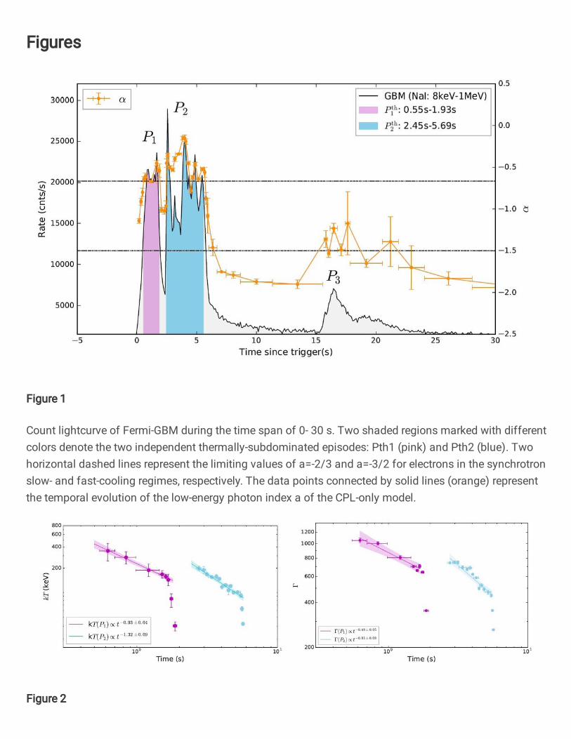
Figures
Figure 1
Count lightcurve of Fermi-GBM during the time span of 0- 30 s. Two shaded regions marked with differentcolors denote the two independent thermally-subdominated episodes: Pth1 (pink) and Pth2 (blue). Twohorizontal dashed lines represent the limiting values of a=-2/3 and a=-3/2 for electrons in the synchrotronslow- and fast-cooling regimes, respectively. The data points connected by solid lines (orange) representthe temporal evolution of the low-energy photon index a of the CPL-only model.
Figure 2

Temporal evolution of the temperature kT (left panel), and bulk Lorentz factor T (right panel). The datapoints indicated by pink and blue colors represent the two different pulses. Solid lines are the best power-law �ts to the data for P1 and P1 excluding several points during the drop, and shaded areas are their 2-o(95% con�dence interval) regions. The derived time-resolved evolution of T is based on the photosphereproperties under the framework of the traditional method22.
Figure 3
Spectrum from 4:95 s to 5:45 s. The spectrum includes data from Fermi-GBM (2 NaI and 1 BGO detector).The �tting is presented by a solid line, including the components of a Plank blackbody function by adashed line and a cutoff power-law by a dotted line.