Embed Size (px)
Citation preview
Ž .Coastal Engineering 41 2000 95–124www.elsevier.comrlocatercoastaleng
A coupling module for tides, surges and waves
Jose Ozer a,), Roberto Padilla-Hernandez b, Jaak Monbaliu b,´ ´Enrique Alvarez Fanjul c, Juan Carlos Carretero Albiach c,
Pedro Osuna b, Jason C.S. Yu b,1, Judith Wolf d
a Management Unit of the North Sea Mathematical Models, Gulledelle 100, B-1200 Brussels, Belgiumb Hydraulics Laboratory, Katholieke UniÕersiteit LeuÕen, de Croylaan 2, B-3001 HeÕerlee, Belgium
c ( )Programa de Clima Marıtimo Ente Publico Puertos del Estado , Antonio Lopez 81, E-28026 Madrid, Spain´ ´ ´d Proudman Oceanographic Laboratory, Bidston ObserÕatory, Birkenhead CH43 7RA, UK
Abstract
A generic module in which tides, surges and waves are incorporated has been developed, testedŽand prepared for dissemination within the framework of the MAST III PROMISE PRe-Oper-
.ational Modelling In the Seas of Europe project. Two existing pre-operational numerical models,a wave model and a hydrodynamic model, were incorporated into a coupling framework thatallows an efficient exchange of information between them. Minimal adaptation of the models wasneeded.
The module has then been implemented and applied to the North Sea, then a series ofexperiments were performed to investigate the sensitivity of waves and surges to coupling. Theseexperiments show that the sensitivity of waves to coupling increases from deep to shallow water.The sensitivity of surges is more uniformly distributed.
The sensitivity of surges to coupling along the Spanish coast was also studied. The modelresults were less sensitive than in the North Sea. This is explained by the relative importance ofthe two forcing components, the atmospheric pressure and the wind stress, in both areas. q 2000Elsevier Science B.V. All rights reserved.
Keywords: Coupling; Surges; Tides; Waves
) Corresponding author. Fax: q32-2-770-6972.Ž .E-mail address: [email protected] J. Ozer .
1 Present address: Department of Marine Environment and Engineering, NSYSU, 70 Lien-Hai Road,Kaoshiung 804, Taiwan.
0378-3839r00r$ - see front matter q2000 Elsevier Science B.V. All rights reserved.Ž .PII: S0378-3839 00 00028-4

( )J. Ozer et al.rCoastal Engineering 41 2000 95–12496
1. Introduction
ŽOne of the many objectives of PROMISE PRe-Operational Modelling In the Seas of.Europe was ‘to rationalise the application of pre-operational tidal, storm, turbulence
and wave models and to determine how these can be improved depending on the rangeof processes incorporated’. To achieve this objective, PROMISE partners have devel-oped generic modules incorporating several processes. These modules have been testedand used in various applications. They are now ready to be disseminated for application
Žin other coastal areas and for broader management applications. Prandle 2000, this.volume gives a general overview, while more detailed information can be found in the
other papers of this volume.ŽFrom the review of existing operational oceanography services Flather, 2000, this
.volume , it is clear that for the time being, wave and storm surge predictions in theNorth Sea are still made separately in most operational centres.
There are, however, several known mechanisms through which each component ofŽ .the total motion affects the others. Heaps 1983 had already identified the need for a
wave model to improve the specification of wind stress in surge models. VariousŽ .interaction mechanisms e.g. the surface drag were identified as potentially important
Ž .Wolf et al., 1988 . Some results from early attempts at coupling are given in Wu andŽ . Ž .Flather 1992 . Tolman 1990 concluded from his investigation into the effects of tides
and storm surges on wind waves that ‘both the instationarity and the inhomogeneity ofdepth and current play a significant role in wave–tide interaction’ and recommendedfurther investigations into the effects of wave–tide interactions on wave heights.
Ž .Mastenbroek et al. 1993 clearly show the influence of a wave-dependent surface dragcoefficient on surge elevations. Even if these surge elevations can be reproduced with an
Žappropriate ‘tuning’ of this parameter in conventional wind stress formulations theŽ . .dimensionless constant a in the Charnock relation Charnock, 1955 in this case , they
argue that ‘a wave-dependent drag is to be preferred for storm surge modelling’. Asummary of the contributions to coupling, up to the end of the WAM project, is given
Ž . Ž .by Burgers et al. 1994 and Cavaleri et al. 1994 .Ž .Davies and Lawrence 1994 notice a significant change of the tidal amplitude and
phase in shallow near-coastal regions due to enhanced frictional effects associated withwind-driven flow and wind wave turbulence.
The development, testing and preparation for dissemination of a generic module inwhich tides, surges and waves are incorporated within the frame of PROMISE, has beenconsidered as a step forward in respect of these studies. The main purpose of this paperis to describe how the module has been developed and to report on a series ofexperiments dealing with the sensitivities of both models to coupling.
In Section 2, the basic tools are briefly described, the modifications imposed by thecoupling are summarised and the way each component may influence the others isdiscussed. In Section 3, the implementation of the models in the North Sea is presented.
Ž .A short discussion on the atmospheric forcing during the test period February 1993Ž .and on the model results when run separately follows. Section 4 deals with the
presentation of the experiments performed to investigate the sensitivity of the models tocoupling and with a detailed investigation of the results of these experiments. While the

( )J. Ozer et al.rCoastal Engineering 41 2000 95–124 97
North Sea is the main area of interest in this paper, there have been other couplingexperiments made during the course of PROMISE. A short overview of the importanceof coupling in the areas where these experiments have been conducted is presented inSection 5. A summary is given and conclusions are drawn in the last section.
2. Development of a generic module for combined modelling of tides, surges andwaves
2.1. Introduction
The following steps have been performed, with the intention of preparing fordissemination, a tool which enables the combined modelling of tides, surges and wavesat the North Sea scale and in shallow water. Firstly, two models were chosen. Secondly,model equations were adapted, where necessary, to account for interactions betweenprocesses. Finally, model codes were modified for an efficient and correct exchange ofinformation. An overview of the two models with a discussion of the modificationsimposed by coupling at the level of model equations is given below. Coding aspects aresubsequently addressed.
2.2. OÕerÕiew of the models
2.2.1. The waÕe modelŽ .The WAM-cycle4 model Gunther et al., 1992; Komen et al., 1994 is now run¨
Ž .operationally at different European centres see Flather, 2000, this volume . It has beenŽused in most of the wave model applications made during the course of PROMISE see,
.Monbaliu et al., 2000, this volume . The only exception is the so-called K-model used inŽ .the Sylt-Rømø applications Schneggenburger et al., 2000, this volume .
The evolution of the wave spectrum, without any presumption on its shape, isŽ .described by the spectral energy balance equation SWAMP group, 1985 . The physics
of wave evolution, for the full set of degrees-of-freedom of a 2D spectrum, isrepresented in accordance to our present knowledge. The governing equation includes
Ž .advection in geographical and spectral direction and frequency space, wind inputŽ . Ž .Janssen, 1989, 1991 , dissipation due to white-capping Gunther et al., 1992 , nonlinear¨
Ž .interactions Hasselmann et al., 1985 and bottom friction. The latter can be computedaccording to different models, ranking from the simplest proposed by Hasselmann et al.Ž . Ž1973 to formulations accounting for a combined wave–current field e.g., Madsen,
.1994; Christoffersen and Jonsson, 1985 .Depth and current refraction are included in the model equations. The interaction of
the waves with the mean flow is implicitly taken into account through the advection inthe frequency space. In the action density balance equation formulated in terms of
Ž .energy Monbaliu et al., 2000, this volume , this term reads
E F E Fs c s c F y c 1Ž . Ž .s s sž /Es s Es s
( )J. Ozer et al.rCoastal Engineering 41 2000 95–12498
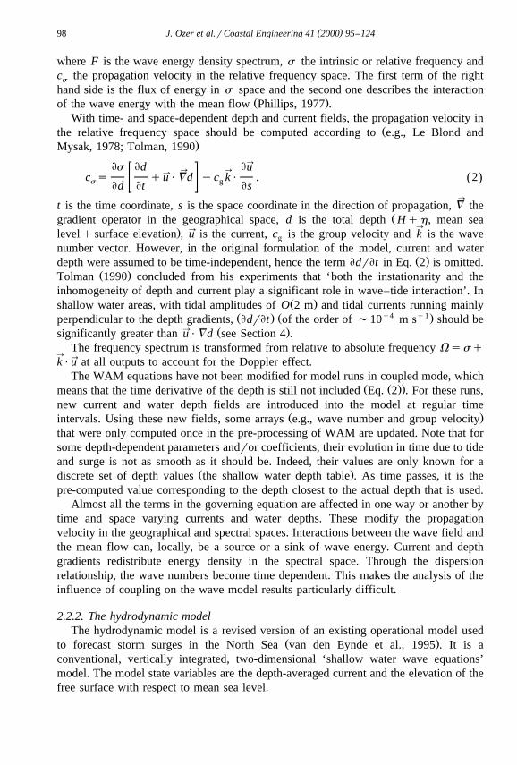
where F is the wave energy density spectrum, s the intrinsic or relative frequency andc the propagation velocity in the relative frequency space. The first term of the rights
hand side is the flux of energy in s space and the second one describes the interactionŽ .of the wave energy with the mean flow Phillips, 1977 .
With time- and space-dependent depth and current fields, the propagation velocity inŽthe relative frequency space should be computed according to e.g., Le Blond and
.Mysak, 1978; Tolman, 1990™Es Ed Eu
™ ™™c s quP=d yc kP . 2Ž .s g
Ed Et Es™
t is the time coordinate, s is the space coordinate in the direction of propagation, = theŽgradient operator in the geographical space, d is the total depth Hqh, mean sea
™™.levelqsurface elevation , u is the current, c is the group velocity and k is the waveg
number vector. However, in the original formulation of the model, current and waterŽ .depth were assumed to be time-independent, hence the term EdrEt in Eq. 2 is omitted.
Ž .Tolman 1990 concluded from his experiments that ‘both the instationarity and theinhomogeneity of depth and current play a significant role in wave–tide interaction’. In
Ž .shallow water areas, with tidal amplitudes of O 2 m and tidal currents running mainlyŽ . Ž y4 y1.perpendicular to the depth gradients, EdrEt of the order of ;10 m s should be
™ Ž .significantly greater than uP=d see Section 4 .The frequency spectrum is transformed from relative to absolute frequency Vssq
™™kPu at all outputs to account for the Doppler effect.The WAM equations have not been modified for model runs in coupled mode, which
Ž Ž ..means that the time derivative of the depth is still not included Eq. 2 . For these runs,new current and water depth fields are introduced into the model at regular time
Ž .intervals. Using these new fields, some arrays e.g., wave number and group velocitythat were only computed once in the pre-processing of WAM are updated. Note that forsome depth-dependent parameters andror coefficients, their evolution in time due to tideand surge is not as smooth as it should be. Indeed, their values are only known for a
Ž .discrete set of depth values the shallow water depth table . As time passes, it is thepre-computed value corresponding to the depth closest to the actual depth that is used.
Almost all the terms in the governing equation are affected in one way or another bytime and space varying currents and water depths. These modify the propagationvelocity in the geographical and spectral spaces. Interactions between the wave field andthe mean flow can, locally, be a source or a sink of wave energy. Current and depthgradients redistribute energy density in the spectral space. Through the dispersionrelationship, the wave numbers become time dependent. This makes the analysis of theinfluence of coupling on the wave model results particularly difficult.
2.2.2. The hydrodynamic modelThe hydrodynamic model is a revised version of an existing operational model used
Ž .to forecast storm surges in the North Sea van den Eynde et al., 1995 . It is aconventional, vertically integrated, two-dimensional ‘shallow water wave equations’model. The model state variables are the depth-averaged current and the elevation of thefree surface with respect to mean sea level.

( )J. Ozer et al.rCoastal Engineering 41 2000 95–124 99
Ž .The model is forced by the tide four semi-diurnal and four diurnal tidal constituentsand the inverse barometric effect along the open boundaries, the atmospheric pressuregradients and the wind stress in the area. A zero normal flux is imposed along the solidboundaries.
Conventional quadratic laws are used to compute surface and bottom stresses. Theequation for the surface stress is
™ ™™ < <t sr C W W 3Ž .s a s
™y3Ž .where r is the air density 1.23 kg m , W is the wind speed at 10 m above the seaa
surface and C is the surface drag coefficient. Various surface drag coefficients aresŽ .proposed in the literature. We generally used the one proposed by Heaps 1965
C s0.565=10y3 for WF5 m sy1s
C s y0.12q0.130W =10y3 for 5-W-19.22 m sy1Ž .s
C s2.513=10y3 for WG19.2 m sy1s
Bottom friction is computed by
™ ™™ ™< <t sr C u uymt 4Ž .b w b s
™y3Ž .where r is the water density 1023 kg m , u is the depth mean current and C is thew bŽ .bottom drag coefficient 0.00243 .
ŽIt is not unusual in 2D storm surge models see for example, Groen and Groves,.1962; Heaps, 1967; Ronday, 1976 to modify the bottom stress so that there is a
Žcomponent directly related to the wind stress a crude way to account for the vertical.structure of the wind-driven current . The coefficient m is generally set equal to 0.1.
Note that this term is introduced into the computation of the surface stress instead of theŽ .bottom friction in the computer code see Section 4 .
Waves can influence the mean flow in three different ways: through the spatialgradients of the radiation stress, by changing the wind stress, and by affecting thebottom friction.
2.2.2.1. Radiation stress. The radiation stress represents the contribution of the wavemotions to the mean horizontal flux of horizontal momentum. It is expressed in terms ofthe wave spectrum. The computation of the radiation stress and its implementation in the
Ž .model equations follows that of Mastenbroek et al. 1993 .
2.2.2.2. Surface stress. The variation of the surface drag with wind speed as shown inŽ .Eq. 3 is an empirical concept that reflects the increase of the sea surface roughness
with increasing wind speed.The wave field largely determines the change of sea surface roughness with wind
speed. There is experimental evidence of a certain dependency between wind stress andŽ .wave age see for example, Maat et al., 1991; Monbaliu, 1994 . In recent years, different
parameterisations for computing the surface stress as function of wind and waves haveŽ .been proposed Makin and Chalikov, 1986; Janssen, 1991 . Janssen’s theory is imple-
mented in WAM-cycle4.
( )J. Ozer et al.rCoastal Engineering 41 2000 95–124100
2.2.2.3. Bottom friction. In shallow waters, the waves interact with the bottom and theorbital motions of the low frequency gravity waves to cause an alternating current in its
Ž .vicinity. This current originates from a thin boundary layer typically a few centimetresin which the level of turbulence is increased, causing an enhancement of the bottom
Ž .stress felt by the current Christoffersen and Jonsson, 1985; Gross et al., 1992 . InWAM-cycle4, bottom dissipation due to the combined effect of current and waves can
Ž .be computed either following the approach proposed by Madsen 1994 or following theŽ .approach proposed by Christoffersen and Jonsson 1985 .
The adaptation of the hydrodynamic model for runs in the coupled mode is asfollows. The spatial derivatives of the radiation stress were introduced in the momentum
Ž .equation. The surface stress is no longer computed according to Eq. 3 but directlytransferred from WAM to the model at regular time intervals. While it is certainly aninteresting subject for further research, the influence of combined waves and currents on
Ž .bottom dissipation for waves andror for currents has not been investigated in theexperiments reported here. To our knowledge, the routines that allow the modelling ofbottom dissipation due to waves and currents still needs to be tested in a realisticconfiguration.
2.3. Coupling procedure
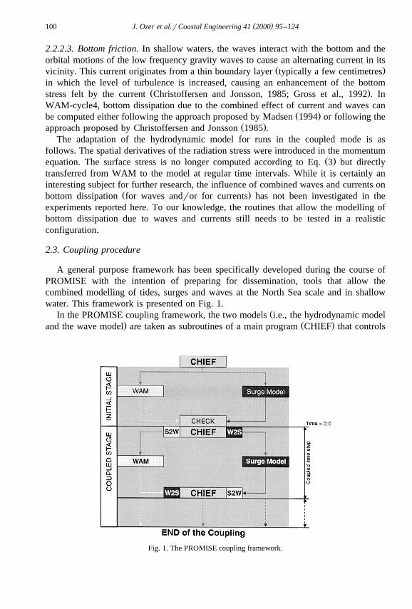
A general purpose framework has been specifically developed during the course ofPROMISE with the intention of preparing for dissemination, tools that allow thecombined modelling of tides, surges and waves at the North Sea scale and in shallowwater. This framework is presented on Fig. 1.
ŽIn the PROMISE coupling framework, the two models i.e., the hydrodynamic model. Ž .and the wave model are taken as subroutines of a main program CHIEF that controls
Fig. 1. The PROMISE coupling framework.

( )J. Ozer et al.rCoastal Engineering 41 2000 95–124 101
their execution. It takes care of the initialisation of both models, and verifies their statusat the start time of coupling. During the coupled mode, it calls the subroutines needed totransfer the information between the two model grids. All North Sea applications havebeen made with this coupling framework.
3. North Sea applications
3.1. Implementation
For the North Sea applications, the two models have been implemented on arelatively coarse grid covering approximately the region 48–718N, 128W–128E. Thebottom topography and coastlines in this area are presented in Fig. 2. The horizontalresolution is equal to 1r28 longitude and 1r38 latitude. The bottom topography is taken
Ž .from the Northeast Atlantic model developed by Flather 1981 .Such an implementation has to be seen as a first step in the development of an
operational model for the forecast of waves, tides and surges in coastal areas. Indeed, itis not unusual to start with such an implementation in a wave forecasting system. Thedesired horizontal resolution in the coastal area of interest is then obtained through
Fig. 2. Model area for the North Sea sensitivity study. Depths are given in metres. The position of the fivestations used for the analysis of time series is also given.

( )J. Ozer et al.rCoastal Engineering 41 2000 95–124102
successive nesting. The same nesting procedure will be later developed for the combinedmodel.
In Fig. 2, the positions of the five stations at which model results are investigated inmore details are also shown. The exact geographical locations of these stations as wellas information on the mean depth and the characteristics of the tidal range are given inTable 1.
Tidal currents at Auk are rather weak. At K13, the tidal ellipse is nearly circular andthe currents are of the order of 0.5 m sy1. At the station Ger, the tidal ellipse is ratherflat with nearly a west–east orientation. Tidal currents are also of the order of 0.5 msy1. A southwest–northeast orientation of tidal currents is observed at both stations Weh
Ž y1 .and Mpn. Tidal currents at station Weh 0.70 m s are nearly two times as large asthose at Mpn.
In the hydrodynamic model, the amplitude and phase of the eight constituents used todefine the tidal forcing are also taken from the Flather’s Northeast Atlantic model. Themodel equations are integrated with a time step equal to 75 s.
In WAM, a logarithmic shallow water depth table contains 63 values starting at adepth of 2 m and increasing successively by a factor of 1.1. The frequency grid is alsologarithmic with f increasing successively by a factor of 1.1. It starts at 0.04 and has 25values. A resolution of 308 is used in the directional space. The source term integrationtime step and the propagation time step are both 600 s. Propagation is computed in a
Ž .quadrant coordinate system see also Monbaliu et al., 2000, this volume .
3.2. Results for a run in uncoupled mode
3.2.1. Reference runIn the first experiment, the models were run without exchanging any information.
This run will be referred to as the reference run. The period for the simulation is themonth of February 1993. The same period has been used for the PROMISE North Sea
Ž .WAM model intercomparison Monbaliu et al., 1997 . An overview of the atmosphericforcing during that month is first given. Model results are discussed afterwards.
3.2.2. Atmospheric conditionsThe atmospheric forcing is taken from the UK Met. Office forecast routinely received
Ž .for storm surge predictions van den Eynde et al., 1995 . For the model runs in hindcast
Table 1Location, mean depth and tidal range at the five stations considered in this study. Note that water depths aretaken from bathymetric data used by the two models at the nearest grid point
Ž . Ž .Station Latitude Longitude Mean depth m Tidal range mX Y X YAuk 56823 59 2803 56 80 0.8X Y X YGer 54830 00 7845 00 21 1.6X Y X YK13 53813 01 3813 12 31 1.2X Y X YMpn 52816 26 4817 46 18 1.2X Y X YWeh 51822 56 2826 20 31 2.8
( )J. Ozer et al.rCoastal Engineering 41 2000 95–124 103
mode, atmospheric pressure and wind speed are available at 6-h intervals, on a 1.258
latituderlongitude grid. Each day, at 00:00 GMT and 12:00 GMT, the informationŽcorresponds to a ‘nowcast’ i.e., a previous model forecast corrected by assimilation of
.in situ observations . At 06:00 GMT and 18:00 GMT, a model forecast is used. A spatialinterpolation is performed to obtain the atmospheric pressure and the wind speed at thegrid-nodes. A linear interpolation is made at each time step in the hydrodynamic model
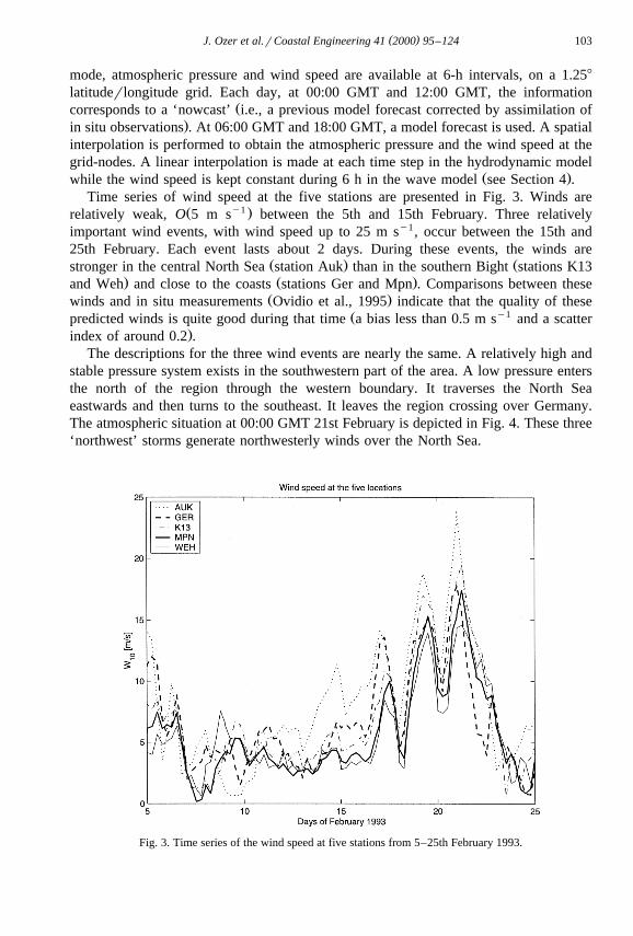
Ž .while the wind speed is kept constant during 6 h in the wave model see Section 4 .Time series of wind speed at the five stations are presented in Fig. 3. Winds are
Ž y1 .relatively weak, O 5 m s between the 5th and 15th February. Three relativelyimportant wind events, with wind speed up to 25 m sy1, occur between the 15th and25th February. Each event lasts about 2 days. During these events, the winds are
Ž . Žstronger in the central North Sea station Auk than in the southern Bight stations K13. Ž .and Weh and close to the coasts stations Ger and Mpn . Comparisons between these
Ž .winds and in situ measurements Ovidio et al., 1995 indicate that the quality of theseŽ y1predicted winds is quite good during that time a bias less than 0.5 m s and a scatter
.index of around 0.2 .The descriptions for the three wind events are nearly the same. A relatively high and
stable pressure system exists in the southwestern part of the area. A low pressure entersthe north of the region through the western boundary. It traverses the North Seaeastwards and then turns to the southeast. It leaves the region crossing over Germany.The atmospheric situation at 00:00 GMT 21st February is depicted in Fig. 4. These three‘northwest’ storms generate northwesterly winds over the North Sea.
Fig. 3. Time series of the wind speed at five stations from 5–25th February 1993.
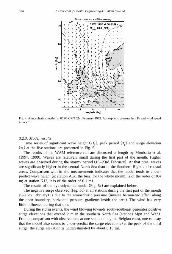
( )J. Ozer et al.rCoastal Engineering 41 2000 95–124104
Fig. 4. Atmospheric situation at 00:00 GMT 21st February 1993. Atmospheric pressure in h Pa and wind speedin m sy1.
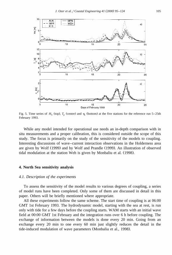
3.2.3. Model resultsŽ . Ž .Time series of significant wave height H , peak period T and surge elevationS p
Ž .h at the five stations are presented in Fig. 5.s
The results of the WAM reference run are discussed at length by Monbaliu et al.Ž .1997, 1999 . Waves are relatively small during the first part of the month. Higher
Ž .waves are observed during the stormy period 16–23rd February . At that time, wavesare significantly higher in the central North Sea than in the Southern Bight and coastalareas. Comparison with in situ measurements indicates that the model tends to under-
Žpredict wave height at station Auk, the bias, for the whole month, is of the order of 0.4.m; at station K13, it is of the order of 0.1 m .
Ž .The results of the hydrodynamic model Fig. 5c are explained below.Ž .The negative surge observed Fig. 5c at all stations during the first part of the month
Ž . Ž5–15th February is due to the atmospheric pressure inverse barometric effect along.the open boundary, horizontal pressure gradients inside the area . The wind has very
little influence during that time.During the storm events, the wind blowing towards south-southeast generates positive
Ž .surge elevations that exceed 2 m in the southern North Sea stations Mpn and Weh .From a comparison with observations at one station along the Belgian coast, one can say
Žthat the model also seems to under-predict the surge elevations at the peak of the third.surge, the surge elevation is underestimated by about 0.15 m .
( )J. Ozer et al.rCoastal Engineering 41 2000 95–124 105
Ž . Ž . Ž .Fig. 5. Time series of H top , T centre and h bottom at the five stations for the reference run 5–25thS p s
February 1993.
While any model intended for operational use needs an in-depth comparison with insitu measurements and a proper calibration, this is considered outside the scope of thisstudy. The focus is primarily on the study of the sensitivity of the models to coupling.Interesting discussions of wave–current interaction observations in the Holderness area
Ž . Ž .are given by Wolf 1999 and by Wolf and Prandle 1999 . An illustration of observedŽ .tidal modulation at the station Weh is given by Monbaliu et al. 1998 .
4. North Sea sensitivity analysis
4.1. Description of the experiments
To assess the sensitivity of the model results to various degrees of coupling, a seriesof model runs have been completed. Only some of them are discussed in detail in thispaper. Others will be briefly mentioned where appropriate.
All these experiments follow the same scheme. The start time of coupling is at 06:00GMT 1st February 1993. The hydrodynamic model, starting with the sea at rest, is runonly with tide for a few days before the coupling starts. WAM starts with an initial wavefield at 00:00 GMT 1st February and the integration runs over 6 h before coupling. Theexchange of information between the models is done every 20 min. Going from anexchange every 20 min to one every 60 min just slightly reduces the detail in the
Ž .tide-induced modulation of wave parameters Monbaliu et al., 1998 .

( )J. Ozer et al.rCoastal Engineering 41 2000 95–124106
Table 2Description of the experiments in which the information is just passed from the hydrodynamic model to thewave model
Experiment Description
Ž .D2W The tide, atmospheric pressure and wind stress computed according to Eq. 3 drive thehydrodynamic model. The tide- and wind-induced water levels are transferred toWAM. Time varying currents are not transferred and therefore have noinfluence on the wave model
TC2W The hydrodynamic model is driven by tide only. Only the tide-induced currents aretransferred to WAM
H2W The hydrodynamic model is driven by the tide, atmospheric pressure and wind stress computedŽ .according to Eq. 3 . Tide- and wind-induced current and water levels are transferred to WAM
The highest level of coupling is when each model has an influence on the otherŽ .two-way coupling . The hydrodynamic model is then driven by the surface stress
Ž Ž ..computed by WAM replacing the surface stress as computed using Eq. 3 , and by theatmospheric pressure and the tide. Tide- and wind-induced currents and water levelsfrom the hydrodynamic model are, in turn, transferred to the wave model. Thisexperiment will be referred to as WH.
Apart from this experiment in the fully coupled mode, others have been made inŽ .which information is just passed from one model to the other one-way coupling . Those
dealing with the sensitivity of waves to current are described in Table 2. The experi-ments dealing with the sensitivity of surge to waves are summarised in Table 3.
The analysis will mainly be based on time series of differences between model resultsŽ .in one experiment and those obtained in the reference run Section 3.2.2 , for three
Ž .parameters significant wave high, peak period and surge elevation at the five stationslisted in Table 1. Computing the value of a global estimator assesses the order ofmagnitude of the differences between two experiments. The global estimator we haveused is defined by
n1 2y t yy tŽ . Ž .Ž .Ý i k r k( n ks1
E y s100 5Ž . Ž .i n12y tŽ .Ý r k( n ks1
Ž .where y is one model parameter, n is the number of values in the time series, y t andi kŽ .y t are the values of y at time t in experiment i and in the reference run,r k k
Table 3Description of the experiment in which the information is just passed from the wave model to thehydrodynamic model
Experiment Description
W2H The hydrodynamic model is driven by the tide, atmospheric pressure and wind stresscomputed by the wave model

( )J. Ozer et al.rCoastal Engineering 41 2000 95–124 107
respectively. Hourly sampled values of model results will be used for the computation ofE.
4.2. SensitiÕity of waÕes, tides and surges to coupling
Ž .While Tolman 1990 mainly investigated the influence of tides and surges on wavesŽ .and Mastenbroek et al. 1993 looked at the influence of a wave-dependent surface stress
Ž .on surges, both effects are combined in our experiment in fully coupled mode WH .Therefore, the results from this experiment are analysed first.
Differences in the model variables between WH and the reference run are presentedin Fig. 6. The values of E for significant wave height, peak period and surge elevationat the five stations computed from 00:00 GMT 5th February–00:00 GMT 25th Februaryare listed in Table 4.
From Table 4, one can say that the coupling introduces, on the average, a change ofless than 5% in significant wave height, and a change of less than 10% in peak periodand surge elevation. As expected, and to some extent hoped, the coupling does not havea strong influence on the model results. After all, both types of model are usedindependently by several operational centres and the reliability of the information theydeliver does not need to be demonstrated again. However, as discussed below, thedifferences are interesting in terms of model behaviour and understanding of the physics.
Sensitivity of wave parameters to coupling increases from deep to shallow water.This fact indicates the need to explore the effects of coupling in shallow coastal waters
Ž . Ž . Ž . Ž .Fig. 6. Time series of differences in H top , T centre and h bottom between the fully coupled run WHS p s
and the reference run at the five stations, 5–25th February 1993.

( )J. Ozer et al.rCoastal Engineering 41 2000 95–124108
Table 4Ž . Ž . Ž .Mean value of H m , T s and h m for the reference run and values of the global estimator, E , forS p s WH
Ž .the differences between the experiment in fully coupled model WH and the reference run at five stationscomputed over the period 5–25th February
² : Ž . ² : Ž . ² : Ž .Station H E H T E T h E hS WH S p WH p s WH s
Auk 2.02 0.6 6.79 1.3 -0.01 9.6Ger 1.30 2.8 5.90 5.2 0.07 7.8K13 1.36 2.0 5.72 3.9 0.02 8.0Mpn 1.01 4.7 6.01 6.8 0.03 8.2Weh 0.86 3.8 5.56 7.7 -0.01 7.2
where modelling with high spatial resolution is needed. Peak period is more sensitivethan significant wave height. Tidal modulation of both wave parameters at all stations is
Ž .clearly visible in the time series of differences almost all of the time Fig. 6 . During thestormy period, wave heights are clearly influenced by coupling. At station Mpn,significant wave height is increased by 38 cm during the third storm. Tide and surgeeffects on waves are further discussed in Section 4.2.
Between the 10–15th February, differences between the wave parameters overrelatively short time intervals resulting from both experiments are as large as thoseobserved during the stormy period. These are noticeable in the time series of differences
Ž .in H and T at stations Ger, K13 and Mpn see Fig. 6 . During these ‘events’, ifS pŽ .significant wave height increase, peak period diminishes see station Ger and vice versa
Ž .see station K13 . At the beginning of such an event, the mean direction of the wavespectrum and that of the wind do not correspond. Currents can accelerate or delay theturning of the wave spectrum towards the direction of the wind. In the formerrlattercase H will grow fasterrslower than without currents. In early stages of wave growth,S
energy is first produced in the high frequency band, then T will shift rapidlyrslowly top
smaller values in the case of acceleratedrdelayed growth. At station Ger, currentsaccelerate the turning and growth of the waves. At station K13, they delay it. How farthese findings can be attributed to the fact that the WAM wave model does not contain a
Ž .linear part in the wind input the so-called Phillips’ term has not been investigated.The hydrodynamic model results seem to be affected more by coupling than the wave
model results. Moreover, even though we observe a small increase in this sensitivityfrom south to north, it seems to be more or less uniformly distributed over all the NorthSea.
Ž .In the time series of differences of surge elevations Fig. 6c , the followingobservations can be made. After 5 days of integration with the atmospheric forcing,some transients are still present in the response of the hydrodynamic model. The winddoes not have a strong influence on the surge elevation before the 15th February.Therefore, after the transients, differences between the two model runs are very small.The influence of the surface stress parameterisation is more obvious during the stormyperiod. The surge elevations in fully coupled mode during a significant period of timeare smaller than in the uncoupled mode especially during the second and third storms.We also observe a modulation of the difference in the surge elevation between the two
Ž .model runs. Results not shown here indicate that this modulation almost disappears

( )J. Ozer et al.rCoastal Engineering 41 2000 95–124 109
when a time interpolation of wind speed is made in WAM. However, according toŽ .Monbaliu et al. 1999 , a linear interpolation in time makes the wave model results less
Ž .accurate peak significant wave heights are generally smaller . The time interpolationŽ .technique proposed by Killworth 1996 for forcing fields of ocean models could help to
solve this problem. With this technique, the mean wind speed felt by the wave modelover 6 h will be as though the wind speed was kept constant, while the surface stresstransferred to the surge model will be smoother. The influence of waves on surges isdiscussed in more detail in Section 4.4.
As the stormy periods are usually of more interest, the analysis of model results inthe following sections will be limited to the period from the 00:00 GMT 16thFebruary–00:00 GMT 23rd February.
4.3. SensitiÕity of waÕes to coupling during storms
4.3.1. OÕerÕiewThe mean values of H for the reference run and the values of the global estimatorS
Ž .E H for the different experiments in which information is transferred from theSŽhydrodynamic model to the wave model including the experiment WH already dis-
.cussed in Section 4.2 are listed in Table 5. The same is done for T in Table 6.pŽ .Comparing the values of Tables 5 and 6 last column with the values of Table 4, it is
remarkable that global estimator values in the latter are larger than in the former. ValuesŽ .of E listed in Table 6 WH are smaller than the values in Table 4 especially for the
peak period. The nearly continuous tidal modulation of wave parameters and the‘events’ observed between the 0 and 15th contribute to these larger values. Part of this
Ž Ž ..also comes from the definition of the global estimator itself Eq. 5 , where, due to thedenominator, periods with small reference signal values are weighted heavier forcomparable difference signals.
From the values listed in both tables above, it can be concluded that coupling has aŽvery small influence on wave model results outside the Southern Bight i.e., above
.538N , at least for the stations considered here. At station Auk, the change in significantwave height and peak period does not exceed 1%. At the stations Ger and K13, thechange in significant wave height is less than 2% and the change in peak period can
Ž .largely be attributed to a local Doppler effect see below . The small influence of
Table 5Ž .Mean value of H m for the reference run and values of the global estimator E for the experiments in whichS
information is transferred from the hydrodynamic model to the wave model. The results reflect the stormyperiod only
² : Ž . Ž . Ž . Ž .Station H E H E H E H E HS D2W S TC2W S H2W S WH S
Auk 3.71 -0.1 0.4 0.6 0.5Ger 2.44 1.4 0.8 2.0 1.2K13 2.70 1.0 1.0 1.8 1.5Mpn 2.09 2.9 3.3 6.1 4.8Weh 1.18 1.3 2.9 3.3 3.0
( )J. Ozer et al.rCoastal Engineering 41 2000 95–124110
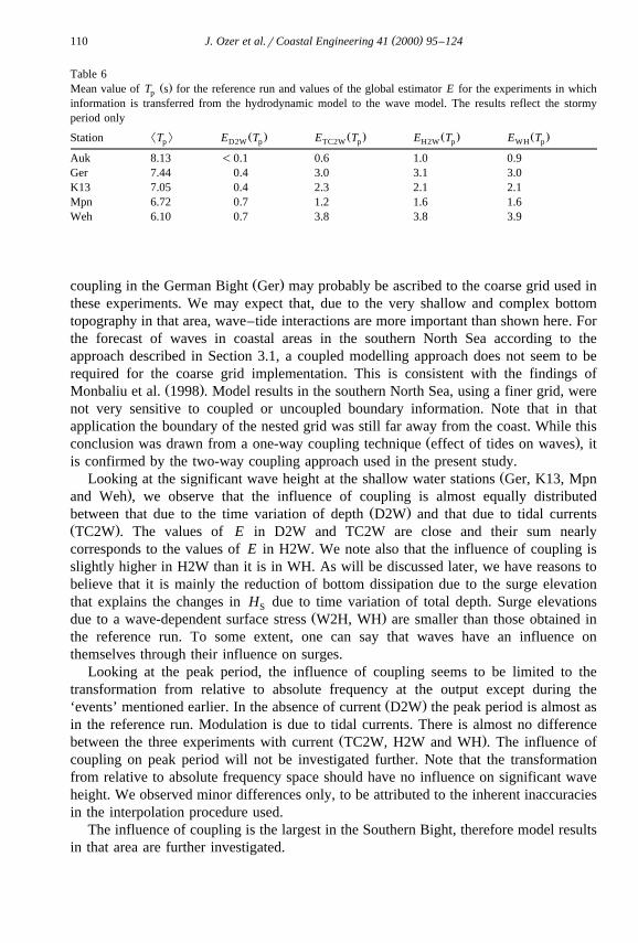
Table 6Ž .Mean value of T s for the reference run and values of the global estimator E for the experiments in whichp
information is transferred from the hydrodynamic model to the wave model. The results reflect the stormyperiod only
² : Ž . Ž . Ž . Ž .Station T E T E T E T E Tp D2W p TC2W p H2W p WH p
Auk 8.13 -0.1 0.6 1.0 0.9Ger 7.44 0.4 3.0 3.1 3.0K13 7.05 0.4 2.3 2.1 2.1Mpn 6.72 0.7 1.2 1.6 1.6Weh 6.10 0.7 3.8 3.8 3.9
Ž .coupling in the German Bight Ger may probably be ascribed to the coarse grid used inthese experiments. We may expect that, due to the very shallow and complex bottomtopography in that area, wave–tide interactions are more important than shown here. Forthe forecast of waves in coastal areas in the southern North Sea according to theapproach described in Section 3.1, a coupled modelling approach does not seem to berequired for the coarse grid implementation. This is consistent with the findings of
Ž .Monbaliu et al. 1998 . Model results in the southern North Sea, using a finer grid, werenot very sensitive to coupled or uncoupled boundary information. Note that in thatapplication the boundary of the nested grid was still far away from the coast. While this
Ž .conclusion was drawn from a one-way coupling technique effect of tides on waves , itis confirmed by the two-way coupling approach used in the present study.
ŽLooking at the significant wave height at the shallow water stations Ger, K13, Mpn.and Weh , we observe that the influence of coupling is almost equally distributed
Ž .between that due to the time variation of depth D2W and that due to tidal currentsŽ .TC2W . The values of E in D2W and TC2W are close and their sum nearlycorresponds to the values of E in H2W. We note also that the influence of coupling isslightly higher in H2W than it is in WH. As will be discussed later, we have reasons tobelieve that it is mainly the reduction of bottom dissipation due to the surge elevationthat explains the changes in H due to time variation of total depth. Surge elevationsS
Ž .due to a wave-dependent surface stress W2H, WH are smaller than those obtained inthe reference run. To some extent, one can say that waves have an influence onthemselves through their influence on surges.
Looking at the peak period, the influence of coupling seems to be limited to thetransformation from relative to absolute frequency at the output except during the
Ž .‘events’ mentioned earlier. In the absence of current D2W the peak period is almost asin the reference run. Modulation is due to tidal currents. There is almost no difference
Ž .between the three experiments with current TC2W, H2W and WH . The influence ofcoupling on peak period will not be investigated further. Note that the transformationfrom relative to absolute frequency space should have no influence on significant waveheight. We observed minor differences only, to be attributed to the inherent inaccuraciesin the interpolation procedure used.
The influence of coupling is the largest in the Southern Bight, therefore model resultsin that area are further investigated.

( )J. Ozer et al.rCoastal Engineering 41 2000 95–124 111
4.3.2. Influence of coupling on H in the Southern BightS
Time series of differences, with respect to the reference run, in H at station K13,S
Mpn and Weh for the different experiments in which information is passed from thehydrodynamic model to the wave model are presented in Fig. 7.
Ž .Coupling seems to have a different influence at the offshore stations K13 and Wehthan it has at the station near the coast. At the offshore stations a clear tidal modulationof significant wave height is seen in all the experiments in which time varying currentsare passed to the wave model. At Mpn, this tidal modulation is less evident.
Ž .In the one way-coupling experiments D2W, TC2W and H2W , the influence ofcoupling increases with the amount of information that is transferred to the wave model.
Ž .With time varying depth D2W , the influence is nearly limited to the two last storms.Ž .With time varying currents TC2W , the tidal modulation is present all the time with an
amplitude that increases with increasing H . Differences in experiment H2W areS
relatively close to the sum of the differences in D2W and TC2W. Wind-induced currentsare generally smaller than tidal currents and, therefore, do not significantly change theinfluence of coupling.
Ž .With time-varying depth only D2W , the propagation speed in the frequency space isŽ Ž .still equal to zero recall that the time derivative of the depth in Eq. 2 is not taken into
.account . There is no interaction between the waves and the mean flow. Depth refractionis time-dependent through the gradients of the sea surface elevation. In the WAM
Ž .model, some wave parameters e.g., wave number, group velocity, phase speed change
Ž . Ž . Ž .Fig. 7. Time series of differences in H at station K13 top , Weh centre and Mpn bottom for all runsS
relevant to the study on the influence of coupling on waves.

( )J. Ozer et al.rCoastal Engineering 41 2000 95–124112
Žonly if the depth variation modifies the shallow water table index while others e.g., the.bottom friction coefficient evolve continuously according to the depth.
In Fig. 7, one may observe that the influence of the time-varying depth is nearlylimited to the two last storms. In the time series of differences in H between D2W andS
the reference run, oscillations at the tidal frequency are not really observed. Therefore,we argue that the effect of the surge elevation dominates over the effect of the tidalelevation in that experiment. This has been further confirmed by an experiment in whichonly the tidal elevations were transferred to the wave model. Model results in thisexperiment were very close to those of the reference run.
During the period of time considered here, neither the tide nor the surge is sufficientto induce a change of the shallow water table index at K13. The wave model at thatstation has used the same index in all the experiments. At Weh, the tidal elevationalready induces a tidal modulation of the index. The same value as in the reference runis used during part of the tidal cycle. A greater value is used during the other part.
Ž .During the two last storms 19th and 21st a greater value is used for the whole day. AtMpn, the index may change due to tide only but not in all tidal cycles and only during asmall part of the tidal period. As at Weh, due to the surge, a greater value is used during19th and 21st. As we observe a strong similarity between the differences at the threestations, we suspect that these variations have had a relatively small influence. There-fore, we have to look for another explanation for the influence of the time varying depth.
In the experiments reported here, bottom dissipation in WAM is computed accordingŽ .to Hasselmann et al. 1973
S syC k ,d E f ,u 6Ž . Ž . Ž .bf bf
with C computed according to:bf
kC k ,h sc 7Ž . Ž .bf sinh 2kdŽ .
where c is a constant set equal to 7.7=10y3 m sy1.In the reference run, a constant depth value is used and the wave number is constant
in time for all frequencies. In experiment D2W, d is continuously changing in time andk may evolve as discussed previously. Time series of C , evaluated at the peakbf
frequency, have been computed for the reference run and for D2W at all stations.Differences in C together with differences in H at the three stations are presented inbf S
Fig. 8. At the three stations, there is a significant correlation between differences in HS
and differences in C . That is not sufficient to assert that differences in H betweenbf S
D2W and the reference run are entirely due to the influence of time varying depth onbottom dissipation but that, at least, it has played an important role.
Tidal modulation of H due to tidal currents is obvious from the results ofS
experiment TC2W.With currents, propagation speeds in the spectral space are no more equal to zero.
Current refraction is taken into account. The interaction between the waves and themean flow is turned on. The currents influence the propagation in the geographical spaceas well. Note that some of these modifications are not applied to all grid points. In themodel code, depth and current gradients in all space directions are computed at gridpoints only if these are surrounded by sea points in both spatial directions. However, at

( )J. Ozer et al.rCoastal Engineering 41 2000 95–124 113
Ž D2W REF . Ž D2W REF . Ž .Fig. 8. Time series of H y H , solid line, and of C yC , dashed line, at station K13 top ,S S bf bfŽ . Ž .Weh centre and Mpn bottom .
grid points adjacent to the coast, depth and current gradients in the direction perpendicu-lar to the coastline are set equal to zero. One can say that the influence of thehydrodynamic model on the wave model is underestimated all along the coastlines.
Depth and current refraction and the interaction between the waves and the meanflow have a local influence at stations K13 and Weh. Due to the resolution of the grid,
Žthe point corresponding to station Mpn is just at a corner coastline on the east side and.on the south side of the mesh . Locally, propagation speeds in the spectral space are
equal to zero and there is no interaction between the waves and the mean flow.At the three stations, differences in H due to the tidal current can be seen as theS
superposition of two main components: one varying with the tidal period and onevarying more slowly in time. The amplitude of both components increases with
Ž .increasing significant wave height. At the two offshore stations K13 and Weh theamplitude of the tidal component is the largest. At Mpn, both components have nearly
Ž .the same amplitude Fig. 7 .Ž .Tolman 1990 suggested that the ‘cumulative effects of wave–tide interactions might
Žoccur for NW winds in particular when the waves and the tide propagate in the same.direction along the British coast for a long period ’. The wind had been blowing from
NW during the stormy period that we have analysed. As the influence of coupling is aslarge, if not greater, at Mpn than it is offshore, we presume that those cumulative effectshave indeed played a role. A complete understanding of the influence of tidal currentson waves in such circumstances cannot be gained by just looking at model results at a

( )J. Ozer et al.rCoastal Engineering 41 2000 95–124114
few points. Nevertheless, such an analysis already provides interesting pieces ofinformation.
Locally, the importance of the wave–tide interactions can be estimated by computingŽ Ž ..time series of the two following terms from Eq. 2
1 Es™
™a s uP=d 8Ž .1s Ed
™c Eu™g
a s kP . 9Ž .2s Es
Ž .Ž .Both terms are frequency-dependent. For the first one, a , 1rs EsrEd decreases1
rapidly, at all depths, with increasing frequency. For a , the range of variation of2Ž . w xc krs is limited to 0.5, 1.0 . Time series have been computed at the peak frequencyg
calculated during the reference run. For a , the calculation is made in the mean direction2
of the wave spectrum determined in the reference run. The mean depth is used to™
™estimate the dot product uP=d. The time series are presented in Fig. 9. At both stations,Ža is significantly greater than a for a mean depth equal to 31.0 m and a peak2 1
y1 Ž .Ž . y1 .frequency equal to 0.1 s , 1rs EsrEd is only of the order of 0.004 m . Clearly,a dominates in the wave–tide interactions. We have verified that the time derivative of2
tidal elevation did not strongly modify the values of a , at least at these two stations.1
The interaction between the waves and the mean flow is, locally, a source of energy,at all frequencies in the mean direction of the spectrum when a is negative and a sink2
Ž TSW REF . Ž . ŽFig. 9. Time series of H y H , solid line and time series of a long dashed line and a shortS S 1 2. Ž . Ž . Ž .dashed line at station K13 top , Weh centre and Mpn bottom . See text for definition of a and a .1 2

( )J. Ozer et al.rCoastal Engineering 41 2000 95–124 115
when it is positive. We observe, in Fig. 9, several periods during which negativerposi-tive values of a correspond to increasingrdecreasing differences in H between2 S
TC2W and the reference run. Clearly, this process plays a role and as it is directlyproportional to the energy density spectrum, it is not surprising to observe increasingmodulation with increasing H .S
Now, positivernegative values of a also correspond to positivernegative propaga-2
tion velocity in the frequency space. Advection in the frequency space is not a directsource or sink of energy. However, a modulation of the wave parameters can be inducedby the adaptation of the spectrum to a new balance.
Ž .We have seen in Section 2 that, sometimes, currents can accelerate or delay theturning of the wave spectrum in the direction of the wind and hence have a significantinfluence on the wave parameters. Apart from these ‘events’, the mean direction of the
Ž .wave spectrum in the experiment with currents TC2W remains relatively close to thatŽ .in the reference run. There are small differences of the order of 28 but no significant
correlation between this angle deviation and the differences in H has been found. Note,S
however, that the resolution in the directional space is equal to 308 and thereforerelatively coarse.
From the values of the global estimator as well as from the figures, results fromŽ .experiment H2W tide- and wind-induced current and elevation passed to WAM has
been found close to the sum of those for experiments D2W and TC2W. This is furtherconfirmed in Fig. 10 where differences in H between H2W and the reference run areS
Ž H2W REF . Ž D2W TC2W REF .Fig. 10. Time series of H y H , solid line, and time series of H q H q2 H , dashedS S S S SŽ . Ž . Ž .line, at station K13 top , Weh centre and Mpn bottom .

( )J. Ozer et al.rCoastal Engineering 41 2000 95–124116
compared to the sum of differences in H for D2W and TC2W. The small discrepanciesS
may come from the non-linearity of the model equations andror from the wind-inducedcurrents.
Ž .Significant wave heights in the experiment in fully coupled mode WH are slightlysmaller than when the information is just passed from the hydrodynamic model to the
Ž .wave model H2W . Surge elevations due to wave-dependent surface stresses onlyŽ .W2H, WH are generally smaller than those obtained in a conventional run of the
Ž . Ž Ž ..hydrodynamic model with surface stress computed according to Heaps 1965 Eq. 3Ž Ž ..and bottom stress modified to have a component directly related to wind stress Eq. 4 .
This is discussed in the following section. Smaller total depths induce more bottomdissipation and hence smaller significant wave height.
4.4. SensitiÕity of surges to waÕes
The influence of wave-dependent surface stress on the surge elevation is investigatedŽ . Ž .with two experiments: W2H one-way coupling and WH two-way coupling . Mean
values of the surge elevation in the reference run and the values for the global estimatorfor the two experiments are listed in Table 7. Time series of differences in h at K13,s
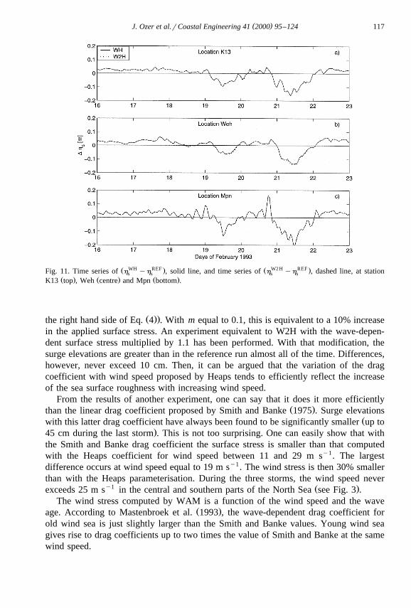
Weh and Mpn are presented in Fig. 11.From Table 7 and Fig. 11, it is clear that the results from both experiments are almost
indistinguishable. While differences in significant wave heights have been observedŽ .between the experiment in fully coupled mode WH and that in one-way coupling
Ž .H2W , this is not the case for surge elevations. In other words, the influence of surgeelevation on the wave fields does not significantly modify the wave-dependent surfacestress.
With respect to the reference run, the surge elevations computed with the wave-de-pendent drag coefficient are slightly greater during the first storm and slightly smaller atthe peak of the two last storms. For the last one, surge elevations with a wave drag
Ž .dependent coefficient are up to 20 cm Mpn below the surge elevations in the referencerun.
Recall that in the reference run of the hydrodynamic model, the bottom stress isŽmodified so as to have a component directly related to the wind stress second term of
Table 7Ž .Mean value of h m for the reference run and values of the global estimator E, for the experiments in whichs
information is transferred from the wave model to the hydrodynamic model. The results reflect the stormyperiod only
² : Ž . Ž .Station h E h E hs W2H s WH s
Auk 0.21 11.4 10.0Ger 0.49 8.1 6.9K13 0.36 8.8 7.7Mpn 0.41 8.5 7.9Weh 0.32 7.9 6.9
( )J. Ozer et al.rCoastal Engineering 41 2000 95–124 117
Ž WH REF . Ž W2H REF .Fig. 11. Time series of h yh , solid line, and time series of h yh , dashed line, at stations s s sŽ . Ž . Ž .K13 top , Weh centre and Mpn bottom .
Ž ..the right hand side of Eq. 4 . With m equal to 0.1, this is equivalent to a 10% increasein the applied surface stress. An experiment equivalent to W2H with the wave-depen-dent surface stress multiplied by 1.1 has been performed. With that modification, thesurge elevations are greater than in the reference run almost all of the time. Differences,however, never exceed 10 cm. Then, it can be argued that the variation of the dragcoefficient with wind speed proposed by Heaps tends to efficiently reflect the increaseof the sea surface roughness with increasing wind speed.
From the results of another experiment, one can say that it does it more efficientlyŽ .than the linear drag coefficient proposed by Smith and Banke 1975 . Surge elevations
Žwith this latter drag coefficient have always been found to be significantly smaller up to.45 cm during the last storm . This is not too surprising. One can easily show that with
the Smith and Banke drag coefficient the surface stress is smaller than that computedwith the Heaps coefficient for wind speed between 11 and 29 m sy1. The largestdifference occurs at wind speed equal to 19 m sy1. The wind stress is then 30% smallerthan with the Heaps parameterisation. During the three storms, the wind speed never
y1 Ž .exceeds 25 m s in the central and southern parts of the North Sea see Fig. 3 .The wind stress computed by WAM is a function of the wind speed and the wave
Ž .age. According to Mastenbroek et al. 1993 , the wave-dependent drag coefficient forold wind sea is just slightly larger than the Smith and Banke values. Young wind seagives rise to drag coefficients up to two times the value of Smith and Banke at the samewind speed.
( )J. Ozer et al.rCoastal Engineering 41 2000 95–124118
Some of the oscillations visible in Fig. 11 have to be attributed to the lack of timeinterpolation on wind speed in WAM. They are significantly reduced when timeinterpolation is performed. Without time interpolation, the behaviour of the wave-depen-dent surface stress is as follows. Each time a new wind field is read, there is a jump in
Ž .the surface stress positive for increasing wind speed, negative otherwise . After that thestress still evolves while the wind speed remains constant. A positive jump is followedby a further increase and then, generally, a decrease. A negative jump is followed by afurther decrease and then, generally, an increase. This reflects the adaptation of the wavespectrum to the wind field.
The conclusions from these experiments do not differ from those drawn by Masten-Ž .broek et al. 1993 . The surge elevations obtained with a wave-dependent drag coeffi-
cient can be reproduced with a conventional quadratic law if an appropriate dragcoefficient is used. Now, a wave-dependent drag coefficient has the practical advantagein that it directly adapts the surface stress to the characteristics of a particular stormevent and to the wave field generated by this storm. It should be therefore preferred.This needs to be confirmed by intensive comparison with in situ data in a wide varietyof storm conditions. If it is confirmed, our experiments show that for surge elevationsthe combined modelling approach is required for the whole area.
Ž .In the experiments made by Mastenbroek et al. 1993 in the North Sea, the radiationstress has a relatively small influence on the calculated water levels. In some cases,however, they observe an increase of 10 to 15 when it is included in the calculation.This shows that it cannot be neglected in all cases. Moreover, it is well known that thisterm is important for applications where depth-induced changes in the waves, asshoaling or breaking, are predominant over propagation and generation, i.e. in coastalareas. It is now included in the momentum equations of the surge model prepared fordissemination and experiments are in progress.
5. Importance of coupling in other areas of interest for PROMISE
During the course of PROMISE project, the interactions between waves and currentshave been studied in areas other than the North Sea.
ŽTheir importance in the Holderness area is discussed at length by Prandle et al. 2000,.this volume . In particular, it is shown that the stronger wave influence is confined to the
shallower parts of this region.Ž .In the Sylt-Rømø Bight Schneggenburger et al., 2000, this volume , a significant
improvement of the hindcast skill of wave period has been obtained by the inclusion ofthe currents.
These studies confirmed that the use of a combined modelling approach becomesmore important in shallow areas with relatively complex bottom topography. Thegeneric module that has been presented in the previous sections should in principle beable to work in such areas.
The influence of various surface stresses on surge elevations along the Spanish coasthas also been investigated. The section of the Spanish coast being studied, and the North

( )J. Ozer et al.rCoastal Engineering 41 2000 95–124 119
Sea are two basins of comparable size but with very different characteristics. Hence, it isof particular interest to compare the sensitivity of surge elevations in both areas.
The effect of coupling along the Iberian Atlantic coast was first explored in AlvarezŽ . Ž .Fanjul et al. 1998 . The wave model used is also WAM-cycle4 WAMDI group, 1988 .
ŽThe hydrodynamic model is the HAMSOM model Backhaus, 1985; Backhaus and.Hainbucher, 1987; Rodriguez et al., 1991; Alvarez Fanjul et al., 1997 . A one-way
coupling approach is followed. The influence of the spatial gradients of the radiationŽ .stress and that of a wave-dependent surface stress Janssen, 1991 on the surge
elevations is investigated. Results show that no practical benefit is obtained. However,the study was limited to a single storm event and, therefore, no possible statisticalconclusions could be derived.
To fill this gap, a similar application covering a longer and very stormy periodŽ .November 1995–March 1996 is performed. The model output are compared and
Žvalidated against measurements from the PROMISE Spanish Coast Data set see Lane et.al., 2000, this volume .
Meteorological wind fields provided by the Instituto Nacional de Meteorologıa and´Ž X .generated by an application of the HIRLAM model 30 resolution are used to force the
WAM model. The model domain covers most of the North Atlantic with a resolutionX Žthat increases up to 10 near the Spanish coasts see Fig. 3 in Carretero Albiach et al.,
.2000, this volume .
Fig. 12. Comparison between wind stress and spatial gradient of radiation stress at one point near La Coruna.˜Then period presented corresponds to the first half of January 1996. Four large storm surge events took placeduring that period.
( )J. Ozer et al.rCoastal Engineering 41 2000 95–124120
The spatial derivatives of the radiation stress derived from the wave spectra are, atthis scale and in deep water, negligible with respect to the wind stress. Time series of
Ž .wind stress and spatial gradient of the radiation stress at one location La Coruna are˜Žpresented in Fig. 12. This result confirms those obtained previously Alvarez Fanjul et
.al., 1998 , but now over a longer period and for a wide variety of storm events. Theresult is therefore more meaningful.
Three model runs were performed with the hydrodynamic model. The model domain,the time step and the other model parameters are as in the surge prediction system
Ždeveloped for the Spanish coast and referred to as NIVMAR see Carretero Albiach et.al., 2000, this volume . In the first run, the wind stress is computed according to Smith
Ž . Ž .and Banke 1975 . In the second run, a Charnock relationship Charnock, 1955 is usedto relate wind stress to wind speed. In the last run, every 6 h, the wind friction velocitycomputed by WAM according to Janssen’s theory is transferred to the hydrodynamicmodel. An interpolation in both time and space is performed.
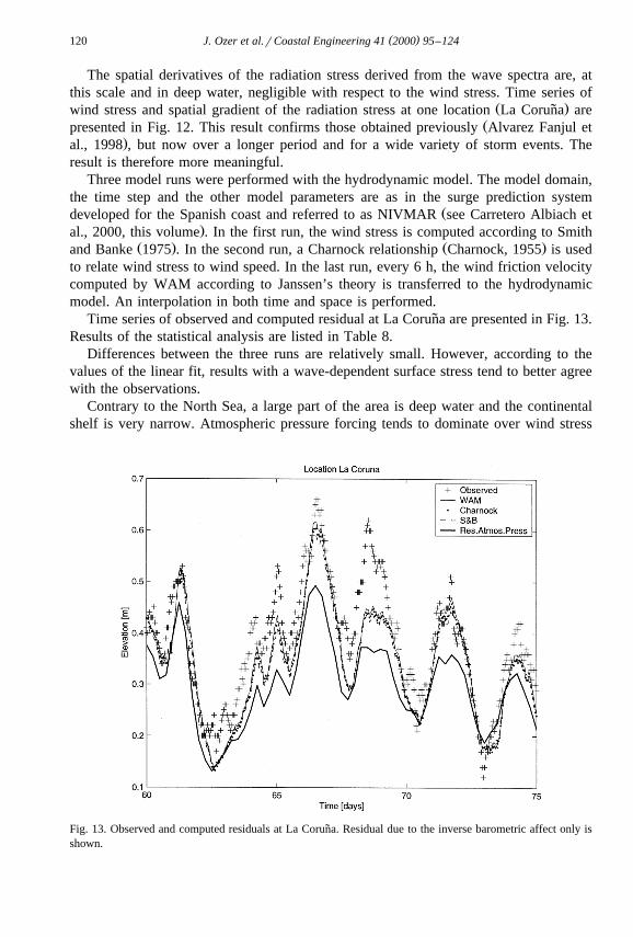
Time series of observed and computed residual at La Coruna are presented in Fig. 13.˜Results of the statistical analysis are listed in Table 8.
Differences between the three runs are relatively small. However, according to thevalues of the linear fit, results with a wave-dependent surface stress tend to better agreewith the observations.
Contrary to the North Sea, a large part of the area is deep water and the continentalshelf is very narrow. Atmospheric pressure forcing tends to dominate over wind stress
Fig. 13. Observed and computed residuals at La Coruna. Residual due to the inverse barometric affect only is˜shown.
( )J. Ozer et al.rCoastal Engineering 41 2000 95–124 121
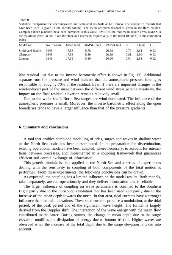
Table 8Statistical comparison between measured and simulated residuals at La Coruna. The number of records that˜have been used is given in the second column. The mean observed residual is given in the third column.Computed mean residuals have been corrected to this value. RMSE is the root mean square error, RMAX isthe maximum error, m and b are the slope and intercept, respectively, of the linear fit and CI is the correlationindex
Ž . Ž . Ž . Ž .Model run No. records Mean cm RMSE cm RMAX m m b cm CI
Smith and Banke 3648 17.58 5.75 20.68 0.79 3.64 0.93Charnock 3648 17.58 5.89 20.69 0.81 3.30 0.92Janssen 3648 17.58 5.80 20.96 0.84 2.88 0.92
Ž .the residual just due to the inverse barometric effect is shown in Fig. 13 . Additionalseparate runs for pressure and wind indicate that the atmospheric pressure forcing isresponsible for roughly 70% of the residual. Even if there are important changes in thewind-induced part of the surge between the different wind stress parameterisations, theimpact on the final residual elevation remains relatively small.
Due to the wider shelf, North Sea surges are wind-dominated. The influence of theatmospheric pressure is small. Moreover, the inverse barometric effect along the openboundaries tends to have a larger influence than that of the pressure gradients.
6. Summary and conclusions
A tool that enables combined modelling of tides, surges and waves in shallow waterat the North Sea scale has been disseminated. In its preparation for dissemination,existing operational models have been adapted, where necessary, to account for interac-tions between processes, and implemented in a coupling framework that guaranteesefficient and correct exchange of information.
This generic module is then applied to the North Sea and a series of experimentsdealing with the sensitivity to coupling of both components of the total motion isperformed. From these experiments, the following conclusions can be drawn.
As expected, the coupling has a limited influence on the model results. Both models,taken separately, are run operationally and they deliver information that is reliable.
The larger influence of coupling on wave parameters is confined to the SouthernBight partly due to the horizontal resolution that has been used and partly due to theincrease of the mean depth towards the north. In that area, tidal currents have a strongerinfluence than the tidal elevations. These tidal currents produce a modulation, at the tidalperiod, of the peak period and of the significant wave height. The former is largelyderived from the Doppler shift. The interaction of the wave energy with the mean flowcontributed to the latter. During storms, the change in mean depth due to the surgeelevation modifies the dissipation of energy due to bottom friction. Higher waves areobserved when the increase of the total depth due to the surge elevation is taken intoaccount.
( )J. Ozer et al.rCoastal Engineering 41 2000 95–124122
In the North Sea, the wind plays a key role in the development of surges. Storm surgemodel results are therefore highly sensitive to wind stress parameterisations. Thissensitivity is almost uniformly distributed in space. Within the North Sea, surgeelevation observed at one location is rarely the consequence of local effect only.Conventional quadratic laws can produce surge elevations similar to those obtained witha wave-dependent surface stress. However, it is necessary that the drag coefficient canaccurately reproduce the increase of the surface roughness with increasing wind speed.In the North Sea experiments reported here, the Heaps’ drag coefficient appears to be abetter candidate than that proposed by Smith and Banke. Since this roughness is stronglycorrelated with the wave field, the wave-dependent surface stress should be preferred instorm surge modelling.
Along the Spanish coast, the shelf is much narrower than in the North Sea.Atmospheric pressure tends to dominate over wind stress in the generation of surgeelevation in that area. Therefore, even if there are considerable changes in the wind-in-duced part due to different wind stress parameterisations, the effect on the final residualremains relatively small.
The increasing importance of coupling when going towards shallower areas has beenconfirmed by the investigations made in the Holderness and the Sylt-Rømø Bight.Further developments of the generic module presented here precisely involve the settingup, for the hydrodynamic model, of a nesting procedure similar to that available inWAM to allow applications in such coastal areas.
Acknowledgements
This study was partially undertaken with financial support from the EU MAST IIIPROGRAMME, contract MAS3-CT9500025. R.A. Flather is thanked for making thebottom topography and some of the results of his Northeast Atlantic model available forthe present study. The authors wish to thank PROMISE partners, in particular D. Prandleand D. van den Eynde for stimulating discussions and useful comments on drafts of thispaper. The comments made by the two anonymous reviewers were very much appreci-ated.
References
Alvarez Fanjul, E., Perez Gomez, B., Rodriguez Sanchez-Arevalo, I., 1997. A description of the tides in theŽ .Eastern North Atlantic. Prog. Oceanogr. 40 1–4 , 217–244.
Alvarez Fanjul, E., Gomez, P., Carretero, J.C., Rodriguez Sanchez-Arevalo, I., 1998. Tide and surge dynamicsŽ .along the Iberian Atlantic Coast. Oceanol. Acta 21 2 , 131–143.
Backhaus, J.O., 1985. A three-dimensional model for simulation of shelf sea dynamics. Dtsch. Hydrogr. Z. 38Ž .4 , 164–187.
Backhaus, J.O., Hainbucher, D., 1987. A finite difference general circulation model for shelf sea and itsapplication to low frequency variability on the North European Shelf. In: Nihoul, J.C.J., Jamart, B.M.Ž .Eds. , Three-dimensional Model of Marine and Estuarine Dynamics. Elsevier Oceanographic Series 45,pp. 221–244.

( )J. Ozer et al.rCoastal Engineering 41 2000 95–124 123
Burgers, G.J.H., Flather, R.A., Jansse, P.A.E.M., Mastenbroek, C., Wu, X., Cavaleri, L., 1994. CombiningŽ .waves and storm surge modelling. In: Komen, G.J. Ed. , Dynamics and Modelling of Ocean Waves.
Cambridge Univ. Press, pp. 371–374.Carretero Albiach, J.C., Alvarez Fanjul, E., Gomez Lahoz, M., Perez Gomez, B., Rodrıguez Sanchez-Arevalo,´ ´
I. et al., 2000. Ocean forecasting in narrow shelf seas: application to the Spanish coasts. Coastal Eng., Thisvolume.
Cavaleri, L., Flather, R.A., Hasselmann, S., Wu, X., 1994. Shoaling and depth refraction. In: Komen, G.J.Ž .Ed. , Dynamics and Modelling of Ocean Waves. Cambridge Univ. Press, pp. 343–348.
Charnock, H. et al., 1955. Wind stress on a water surface. Q. J. R. Meteorol. Soc. 81, 639–640.Christoffersen, J.B., Jonsson, I.G., 1985. Bed friction and dissipation in a combined current and wave motion.
Ocean Eng. 12, 387–423.Davies, A.M., Lawrence, J., 1994. Examining the influence of wind and wave turbulence on tidal currents,
using a three-dimensional hydrodynamic model including wave–current interaction. J. Phys. Oceanogr. 24,2441–2460.
Flather, R.A., 1981. Results from a model of the north east Atlantic relating to the Norwegian Coastal Current.Ž .In: Sætre, R., Mork, M. Eds. , The Norwegian Coastal Current, Proceedings of the Norwegian Coastal
Current Symposium, Geilo, 9–12 September 1980 vol. II, pp. 427–458.Flather, R.A., 2000. Existing operational oceanography. Coastal Eng., This volume.
Ž .Groen, P., Groves, G.W., 1962. Surges. In: Hill, M.N. Ed. , The Sea vol. 1 Wiley, New York, NY, pp.611–646.
Gross, T.F., Isley, A.E., Sherwood, C.R., 1992. Estimation of stress and bed roughness during storms on theŽ .Northern California Shelf. Cont. Shelf Res. 12 2r3 , 389–413.
Gunther, H., Hasselmann, S., Janssen, P.A.E.M., 1992. The WAM model Cycle 4. Report No. 4, Hamburg.¨Hasselmann, K., Barnett, T.P., Bouws, E., Carlson, H., Cartwright, D.E., Enke, K., Ewing, J.I., Gienapp, H.,
Hasselmann, D.E., Kruseman, P., Meerbrug, A., Muller, P., Olbers, D.J., Richter, K., Sell, W., Walden,¨H., 1973. Measurements of wind-wave growth and swell decay during the Joint North Sea Wave ProjectŽ . Ž .JONSWAP . Dtsch. Hydrogr. Z. A8 12 , 95 pp.
Hasselmann, S., Hasselmann, K., Allender, J.H., Barnett, T.P., 1985. Computations and parameterizations ofthe nonlinear energy transfer in a gravity-wave spectrum: Part. II. Parameterizations of the nonlinearenergy transfer for application in wave models. J. Phys. Oceanogr. 15, 1378–1391.
Heaps, N.S., 1965. Storm surges on a continental shelf. Philos. Trans. R. Soc. London, Ser. A 257, 351–383.Ž .Heaps, N.S., 1967. Storm surges. In: Barnes, H. Ed. , Oceanography and Marine Biology Annual Review.
Allen and Urwin, London, pp. 11–47.Heaps, N.S., 1983. Storm surges 1967–1982. Geophys. J. R. Astron. Soc. 74, 331–376.Janssen, P.A.E.M., 1989. Wave-induced stress and the drag of the air flow over sea waves. J. Phys. Oceanogr.
19, 745–754.Janssen, P.A.E.M., 1991. Quasi-linear theory of wind-wave generation applied to wave forecasting. J. Phys.
Oceanogr. 21, 1631–1642.Killworth, P.D., 1996. Time interpolation of forcing fields in ocean models. J. Phys. Oceanogr. 26, 136–143.Komen, G.J., Cavaleri, L., Donelan, M., Hasselmann, K., Hasselmann, S., Janssen, P.A.E.M., 1994. Dynamics
and Modelling of Ocean Waves. Cambridge Univ. Press, Cambridge, 532 pp.Lane, A., Riethmuller, R., Herbers, D., Rybaczok, P., Gunther, H., Baumert, H., 2000. Observational data sets¨ ¨
for model development. Coastal Eng., This volume.Le Blond, P.H., Mysak, L.A., 1978. Waves in the Ocean. Elsevier, Amsterdam.Maat, N., Kraan, C., Oost, W.A., 1991. The roughness of wind waves. Boundary Layer Meteorol. 54, 89–103.Madsen, O.S., 1994. Spectral wave–current bottom boundary layer flows. Proceedings of the 24th Interna-
tional Conference on Coastal Engineering. Coastal Engineering Research CouncilrASCE, Kobe, pp.384–398.
Makin, V.K., Chalikov, D.V., 1986. Calculating momentum and energy fluxes going into developing waves.Izv., Atmos. Ocean Phys. 22, 1015–1019.
Mastenbroek, C., Burgers, G., Janssen, P.A.E.M., 1993. The dynamical coupling of a wave model and a stormsurge model through the atmospheric boundary layer. J. Phys. Oceanogr. 23, 1856–1866.
Monbaliu, J., 1994. On the use of the Donelan wave spectral parameter as a measure for the roughness of windwaves. Boundary Layer Meteorol. 67, 277–291.

( )J. Ozer et al.rCoastal Engineering 41 2000 95–124124
Monbaliu, J., Zhang, M.Y., de Bakker, K., Hargreaves, J., Luo, W., Flather, R., Carretero, J.C., Gomez Lahoz,M., Lozano, I., Stawartz, M., Gunther, H., Rosenthal, W., Ozer, J., 1997. WAM model intercomparisons¨— North Sea. Proudman Oceanographic Laboratory Report No. 47.
Monbaliu, J., Yu, C.S., Osuna, P., 1998. Sensitivity of wind-wave simulation to coupling with a tidersurgemodel — with application to the southern North Sea. Proceedings of the 26th International Conference onCoastal Engineering, Copenhagen. pp. 945–957.
Monbaliu, J., Hargreaves, J., Carretero, J.-C., Gerritsen, H., Flather, R., 1999. Wave modelling in thePROMISE project. Coastal Eng., 379–407, special issue on SCAWVEX.
Monbaliu, J., Padilla-Hernandez, R., Hargreaves, J.C., Carretero Albiach, J.C., Luo, W., Sclavo, M., Gunther,´ ¨H., 2000. The spectral wave model WAM adapted for applications with high spatial resolution. CoastalEng., This volume.
Ovidio, F., Bidlot, J.R., van den Eynde, D., 1995. Validation and improvement of the quality of theoperational wave model MU-WAVE by the use of ERS-1 satellite data, MUMMrT3rAR05. Final ReportEuropean Space Agency Pilot Project PP2-B9.
Phillips, O.M., 1977. The Dynamics of the Upper Ocean. Cambridge Univ. Press, 336 pp.Prandle, D., 2000. Operational oceanography in coastal waters. Coastal Eng., This volume.Prandle, D., Hargreaves, J.C., McManus, J.P., Campbell, A.R., Duwe, K., Lane, A., Mahnke, P., Shimwell, S.,
Wolf, J., 2000. Tide, wave and suspended sediment modelling on an open coast — Holderness. CoastalEng., This volume.
Rodriguez, I., Alvarez, E., Krohn, J., Backhaus, J., 1991. A mid-scale tidal analysis of waters around thenorth-western corner of the Iberian Peninsula. Proceedings book from ‘Computer modelling in oceanengineering 91’, Balkema.
Ronday, F.C., 1976. Modeles hydrodynamiques. Projet Mer, Rapport Final, Services du Premier Ministre,`Programmation de la Politique Scientifique, Brussels, Belgium, 270 pp.
Schneggenburger, C., Gunther, H., Rosenthal, W., 2000. Spectral wave modelling with non-linear dissipation:¨validation and application in a coastal tidal environment. Coastal Eng., This volume.
Smith, S.D., Banke, E.G., 1975. Variation of the sea surface drag coefficient with wind speed. Q. J. R.Meteorol. Soc. 101, 665–673.
Ž .SWAMP group, 1985. Sea wave modelling project SWAMP . An intercomparison study of wind wavepredictions models: Part 1. Principal results and conclusions. Ocean Wave Modelling. Plenum, New York,256 pp.
Tolman, H.L., 1990. Wind wave propagation in tidal seas. Commun. Hydraul. Geotech. Eng., January, DelftUniversity of Technology, 135 pp.
van den Eynde, D., Scory, S., Malisse, J.-P., 1995. Operational modelling of tides and waves in the North Seaon the Convex C230 at MUMM. European Convex User’s Conference 1995, 24–27 October 1995,Brussels, Belgium.
WAMDIgroup, 1988. The WAM model — a third generation ocean wave prediction model. J. Phys.Oceanogr. 18, 1775–1810.
Wolf, J., 1999. The estimation of shear stresses from near-bed turbulent velocities for combined wave–currentflows. Coastal Eng. 37, 529–543.
Wolf, J., Prandle, D., 1999. Some observations of wave–current interaction. Coastal Eng. 37, 471–485.Wolf, J., Hubbert, K.P., Flather, R.A., 1988. A feasibility study for the development of a joint surge and wave
model. Proudman Oceanographic Laboratory Report No. 1, 109 pp.Wu, X., Flather, R.A., 1992. Hindcasting waves using a coupled wave–tide-surge model. Third International
Workshop on Wave hindcasting and forecasting, Montreal, Quebec, May 19–22. pp. 159–170, Environ-ment Canada, Prepints.


![Switching Surges Handout[1]](https://img.pdfslide.net/doc/110x75/5439dc86afaf9fbd2e8b5532/switching-surges-handout1.jpg)