A Crash Course in Geometric Algebra and Geometric Calculus · geometric algebra and geometric calculus, somewhat in the spirit of Alan Macdonald’s A Survey of Geometric Algebra

A Crash Course in Geometric Algebra andGeometric Calculus

M. D. TaylorProfessor Emeritus

Department of MathematicsUniversity of Central Florida

Orlando, FL 32816-1364E-mail: [email protected]

Copright c©Michael D. Taylor 2013, 2014

Contents

Introduction iii

1 Simple k-Vectors 11.1 Definition . . . . . . . . . . . . . . . . . . . . . . . . . . . . . . . 11.2 Operations with simple k-vectors . . . . . . . . . . . . . . . . . . 7

2 The Space of k-Vectors 112.1 The vector space ΛkRn . . . . . . . . . . . . . . . . . . . . . . . . 112.2 Wedge product . . . . . . . . . . . . . . . . . . . . . . . . . . . . 122.3 Bases for ΛkRn . . . . . . . . . . . . . . . . . . . . . . . . . . . . 132.4 Reversion and dot product . . . . . . . . . . . . . . . . . . . . . . 14

3 Calculus With k-Vectors 173.1 Hyperplanes . . . . . . . . . . . . . . . . . . . . . . . . . . . . . . 173.2 Differentiability . . . . . . . . . . . . . . . . . . . . . . . . . . . . 193.3 Surfaces and tangent vectors . . . . . . . . . . . . . . . . . . . . 203.4 Tangent blades and orientation . . . . . . . . . . . . . . . . . . . 233.5 Integrals . . . . . . . . . . . . . . . . . . . . . . . . . . . . . . . . 24

4 Geometric Algebra 284.1 Gn and grades . . . . . . . . . . . . . . . . . . . . . . . . . . . . 284.2 The geometric product . . . . . . . . . . . . . . . . . . . . . . . . 294.3 Extending reversion . . . . . . . . . . . . . . . . . . . . . . . . . 304.4 The scalar product . . . . . . . . . . . . . . . . . . . . . . . . . . 314.5 The wedge product of multivectors . . . . . . . . . . . . . . . . . 324.6 Division by multivectors . . . . . . . . . . . . . . . . . . . . . . . 334.7 Reciprocal vectors . . . . . . . . . . . . . . . . . . . . . . . . . . 35

i

CONTENTS ii

5 Derivatives and the Fundamental Theorem 365.1 Directional derivatives . . . . . . . . . . . . . . . . . . . . . . . . 365.2 The geometric derivative . . . . . . . . . . . . . . . . . . . . . . . 385.3 Oriented integrals . . . . . . . . . . . . . . . . . . . . . . . . . . 405.4 Induced orientation . . . . . . . . . . . . . . . . . . . . . . . . . . 415.5 The Fundamental Theorem . . . . . . . . . . . . . . . . . . . . . 44

Introduction

These notes are meant to be a quick introduction to some of the ideas ofgeometric algebra and geometric calculus, somewhat in the spirit of AlanMacdonald’s A Survey of Geometric Algebra and Geometric Calculus, [6].Macdonald’s paper can be obtained free at the indicated web address, ittouches on topics which we do not cover, and it is highly recommended.

This is a Crash Course in that it is meant to be quick and superficial withessentially all proofs omitted. We hope that these notes will, nevertheless,give the reader some feel (however inadequate) for how geometric algebraand geometric calculus work.

The plan at this point is that this superficial crash course will be eventuallyfollowed by a much more detailed work [12].

In the meantime, the impatient reader who wants to get into the meat ofthe topic can consult the two introductory books [8] and [9] by Macdonald, thevolume [3] by Hestenes and Sobczyk which is often considered the “bible” forthis material, or a recent book [11] by Sobczyk. Those who would like to seean introductory book aimed at physicists may wish to look at [2] by Doranand Lasenby. There is also a set of online notes by Alan Bromborsky, [1],that seems aimed at a general mathematical audience.

The reader should have a modest acquaintance with linear algebra and aknowledge of multivariable calculus as presented in an introductory calculuscourse.

We shall use Greek letters, α, β, χ, η, and so forth for real numbers andLatin letters, a, b, x, y, z, etc. for vectors and multivectors. The symbol Rstands for the set of real numbers and Rn for the set of ordered n-tuples ofreal numbers. Given x = (χ1, . . . , χn) in Rn, sometimes we think of this as apoint, sometimes as a vector, depending on what we want to do.

iii

INTRODUCTION iv

Also, in Rn, we shall use the symbols e1, . . . , en for the standard basisvectors. That is, ei is the unit vector in the positive direction parallel to theith-axis in Rn. Thus in R3,

e1 = (1, 0, 0),

e2 = (0, 1, 0),

e3 = (0, 0, 1).

Chapter 1

Simple k-Vectors

Our first step in understanding geometric algebra is to construct what arecalled k-vectors. In this chapter we look at special kinds of k-vectors, thesimple k-vectors, which have a very nice geometrical interpretation. We movein the next chapter to general k-vectors.

Our presentation is rapid and superficial. Details about the constructionof k-vectors and a number of proofs of their properties can be found in [5],The Wedge Product and Analytic Geometry, and in [12] (when it appears). Alink to a copy of [5] can be found online at http://www.mdeetaylor.com/

?page_id=286.

1.1 DefinitionA vector x = (χ1, . . . , χn) in Rn will also be referred to by us as a 1-vector.It is usual to picture a vector (1-vector) as a directed line segment. This isuseful for applications and helpful for the intuition.

Any two directed line segments are said to represent the same vector pro-vided they have the same magnitude, direction, and orientation with respectto that direction. All such directed line segments may be considered to startat the origin; if you translate a directed line segment without altering itslength, direction, or orientation, then it is considered to repesent the samevector. If we consider Figugre 1.1, then a and b represent the same vector.On the other hand, c represents a different vector than a because, althoughit has the same direction as a in the sense that it is parallel to a, it is ori-ented in the opposite direction. And d is not the same vector as a because it

1

CHAPTER 1. SIMPLE K-VECTORS 2

a be

c

d

Figure 1.1: Vectors as directed line segements

has a different magnitude (length), while e is different because it points in adifferent direction from a.

We want to introduce the idea of a k-vector where k = 0, 1, 2, 3, . . ..Actually, what we shall discuss at this point is simple k-vectors.

The 1-vectors are just what we ordinarily think of as vectors. By 0-vectors,we mean scalars, that is, real numbers.

To see what we mean by a simple 2-vector, notice that if we choose twovectors a1 and a2 in Rn, they determine a parallelogram. (Figure 1.2.) We

a1

a2

Figure 1.2: A simple 2-vector

think of this as being a representative of a simple 2-vector much in the sensein which we thought of a directed line segment as representing a vector. Thesymbol we use for this simple 2-vector is

a1 ∧ a2.Just as with 1-vectors, we may think of simple 2-vectors as constructed fromvectors starting at the origin. If we translate the associated parallelogramto a different location—translation in which we are careful not to rotate theparallelogram out of its defining plane—then it still represents the samesimple 2-vector.

The three properties we associated with directed line segments haveanalogs here: magnitude, direction, orientation.


By the magnitude of a1 ∧ a2, we mean the area of the associated paral-lelogram. It turns out that the area of the parallelogram is given by

magnitude of a1 ∧ a2 =

√det

(a1 • a1 a2 • a1a1 • a2 a2 • a2

)where ai • aj is the dot product of ai and aj . (The knowledgeable readermay note that this looks suggestive of the distance formula in n-dimensionalgeometry. It should, and it generalizes.)

When we talk about two simple 2-vectors—say, a1 ∧ a2 and b1 ∧ b2—thenthe analog to having the same direction is that they must both lie in the sameplane, that is, in the same two-dimensional vector subspace V of Rn. (SeeFigure 1.3.) If they do not lie in the same two-dimensional vector subspace,

a1

a2b2

b1

V

Figure 1.3: a1 ∧ a2 and b1 ∧ b2 lying in V

then they are considered to “have different directions.”As for orientation, this is analogous to both simple 2-vectors being “right-

handed” or “left-handed.” The orientations of a1 ∧ a2 and b1 ∧ b2 can onlybe compared if they both lie in the same two-dimensional vector subspace.The reason for this is that if you pick a1 ∧ a2 up out of the plane in whichit lives, flip it over in 3-dimensional space, and drop it back into the plane,as in Figure 1.4, then it switches from being “right-handed” to “left-handed”and is now written as a2 ∧ a1.

If one has two simple 2-vectors a1 ∧ a2 and b1 ∧ b2 lying in the same two-dimensional vector subspace V , then to see if they have the same orientationor not, one checks the sign of

det

(a1 • b1 a2 • b1a1 • b2 a2 • b2

). (1.1)


Flip!

a1

a2

−a1

a2a1 ∧ a2

a2 ∧ a1

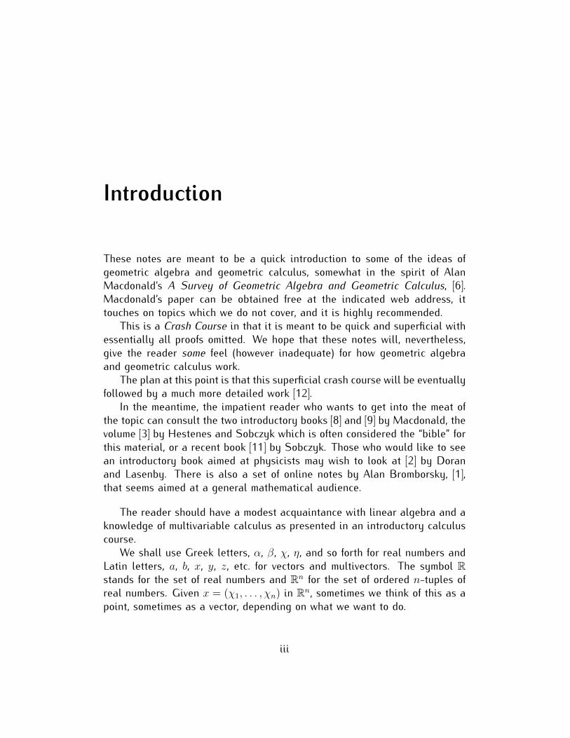
Figure 1.4: “Flipping” a 2-vector to change its orientation

If this is positive, then a1 ∧ a2 and b1 ∧ b2 are considered to have the sameorientation; if it is negative, they have opposite orientations. If (1.1) is zero,then the parallelogram of one of the two simple 2-vectors (or perhaps both ofthem) must be degenerate, that is, a figure of zero area. If a1 ∧ a2 and b1 ∧ b2lie in different planes, then we consider their orientations to be incomparable.Notice that the order in which a1 and a2 occur in the expression a1∧a2 playsan important role here, and it is easy to check that unless the parallelogramis degenerate, a1 ∧ a2 and a2 ∧ a1 must always have opposite orientations.

Now here is the important point:We consider a1∧a2 and b1∧ b2 to be the same simple 2-vector if and only

if they have the same magnitude (area), direction (lie in a common plane),and orientation (handedness).

These considerations may be generalized to define simple k-vectors.Suppose we have an ordered k-tuple (a1, . . . , ak) of vectors in Rn; that

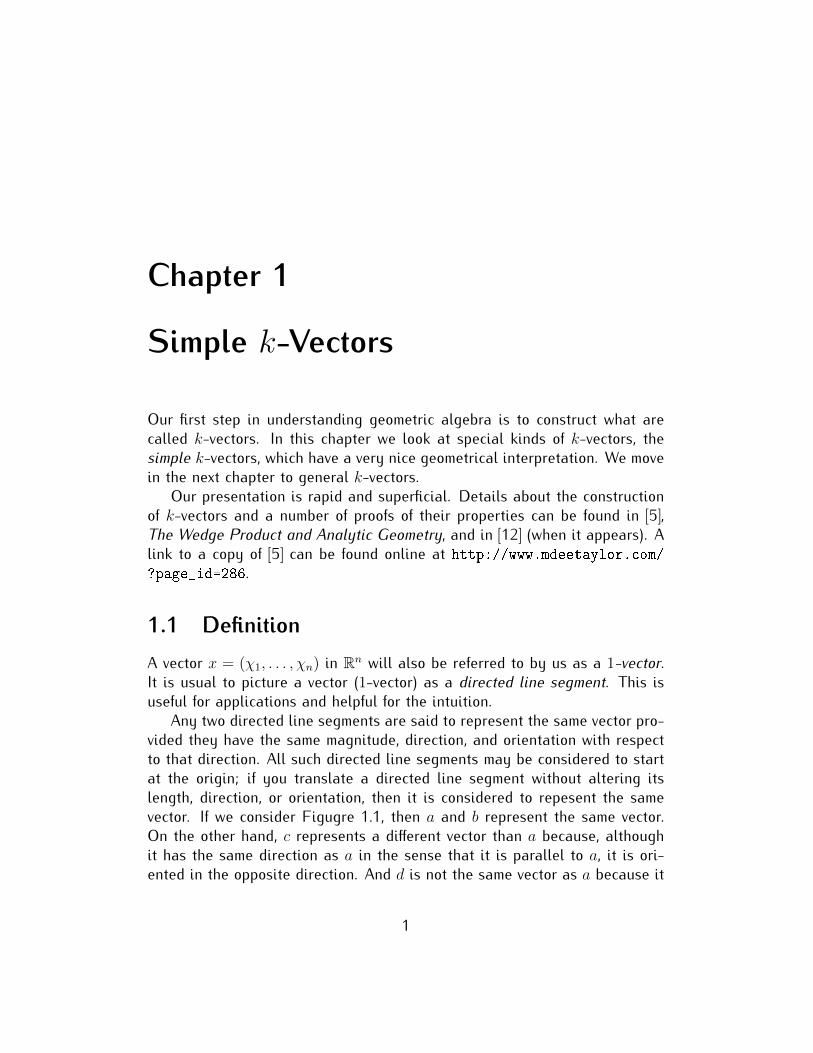
is, each ai is a vector in Rn so can presumably be written in the form ai =(λi1, . . . , λin) where each λij is a real number. Each such ordered k-tuplegenerates a k-dimensional parallelepiped having a1, . . . , ak as its edges. (SeeFigure 1.2 for k = 2. For k = 3, see Figure 1.5.)

We leave it to the reader to play with the idea that each x in Rn is a pointof the parallelepiped if and only if we can write x (considered as a vector)in the form x = τ1a1 + · · · + τkak for some choice of scalars τ1, . . . , τk where0 ≤ τi ≤ 1 for each i. The vertices of the parallelepiped are those pointswhere the scalars τi are all chosen to be 0 or 1.

Given a parallelepiped with edges a1, . . . , ak, we take its k-dimensional


a1

a2

a3

Figure 1.5: 3-dimensional parallelepiped

volume to be

vol(a1, . . . , ak)def.=

√√√√√det

a1 • a1 · · · a1 • ak· · ·

ak • a1 · · · ak • ak

.This always turns out to be a nonnegative real number.

Of course,

1-dimensional volume = length,2-dimensional volume = area.

If vol(a1, . . . , ak) = 0, then we say that the parallelepiped is degenerate. Onecan show that the parallelepiped with edges a1, . . . , ak is degenerate preciselywhen a1, . . . , ak are linearly dependent vectors. Thus the parallelogram withedges a1 and a2 is nondegenerate if and only if the parallelogram has positivearea.

Now to generalize orientation. To do this, we want to think of a k-dimensional parallelepiped as being an ordered k-tuple of vectors (a1, . . . , ak).Each ai is an edge. The order in which they are written determines the ori-entation.

We do not directly define orientation; rather we define what it means tosay that two k-parallelepipeds (a1, . . . , ak) and (b1, . . . , bk) to have the sameorientation. This is sufficient for our purposes.

1. If {a1, . . . , ak} and {b1, . . . , bk} are both linearly dependent sets, then(a1, . . . , ak) and (b1, . . . , bk) are considered to have the same orientation,the 0-orientation.


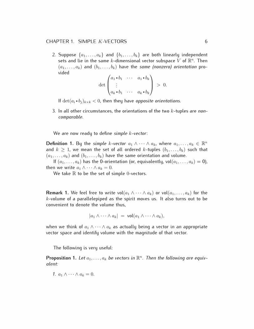
2. Suppose {a1, . . . , ak} and {b1, . . . , bk} are both linearly independentsets and lie in the same k-dimensional vector subspace V of Rn. Then(a1, . . . , ak) and (b1, . . . , bk) have the same (nonzero) orientation pro-vided

det

a1 • b1 · · · a1 • bk...

ak • b1 · · · ak • bk

> 0.

If det(ai • bj)k×k < 0, then they have opposite orientations.

3. In all other circumstances, the orientations of the two k-tuples are non-comparable.

We are now ready to define simple k-vector :

Definition 1. By the simple k-vector a1 ∧ · · · ∧ ak, where a1, . . . , ak ∈ Rn

and k ≥ 1, we mean the set of all ordered k-tuples (b1, . . . , bk) such that(a1, . . . , ak) and (b1, . . . , bk) have the same orientation and volume.

If (a1, . . . , ak) has the 0-orientation (or, equivalently, vol(a1, . . . , ak) = 0),then we write a1 ∧ · · · ∧ ak = 0.

We take R to be the set of simple 0-vectors.

Remark 1. We feel free to write vol(a1 ∧ · · · ∧ ak) or vol(a1, . . . , ak) for thek-volume of a parallelepiped as the spirit moves us. It also turns out to beconvenient to denote the volume thus,

|a1 ∧ · · · ∧ ak| = vol(a1 ∧ · · · ∧ ak),

when we think of a1 ∧ · · · ∧ ak as actually being a vector in an appropriatevector space and identify volume with the magnitude of that vector.

The following is very useful:

Proposition 1. Let a1, . . . , ak be vectors in Rn. Then the following are equiv-alent:

1. a1 ∧ · · · ∧ ak = 0.


2. a1, . . . , ak are linearly dependent.

3. vol(a1 ∧ · · · ∧ ak) = |a1 ∧ · · · ∧ ak| = 0.

Similarly, these conditions are equivalent:

1. a1 ∧ · · · ∧ ak 6= 0.

2. a1, . . . , ak are linearly independent.

3. vol(a1 ∧ · · · ∧ ak) = |a1 ∧ · · · ∧ ak| > 0.

1.2 Operations with simple k-vectorsWe define three operations with simple k-vectors: Multiplication by a scalar(a real number), the dot product, and the wedge product.

It should be noted that though we use the word “vector” in the expression“simple k-vector,” these are not really vectors at all, at least not in the senseof belonging to a vector space. The problem is that we have no operation ofaddition. We shall remedy this lack in the next chapter.

Definition 2. For λ ∈ R and a k-blade a1∧· · ·∧ak, we define λ(a1∧· · ·∧ak) =a1 ∧ · · · ∧ λai ∧ · · · ∧ ak for i = 1, . . . , k. By −a1 ∧ · · · ∧ ak we shall mean(−1)(a1 ∧ · · · ∧ ak).

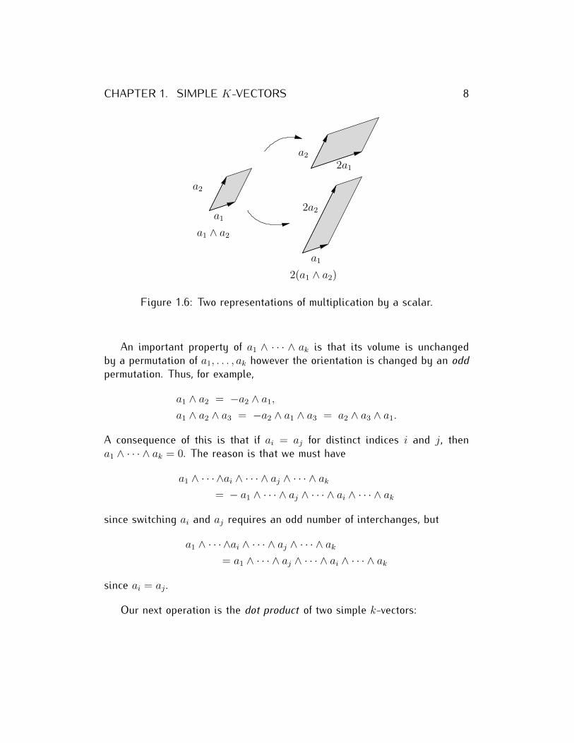
In Figure 1.6 we show two different ways we can represent 2(a1 ∧ a2)as an oriented parallelogram. Of course the two oriented parallelograms areequivalent.

Scalar multiplication has an obvious geometric interpretation: If you mul-tiply one edge of an oriented parallelepiped by λ, then the volume changesby a factor of |λ|. Thus

vol(λ(a1 ∧ · · · ∧ ak)

)= vol(a1 ∧ · · · ∧ λai ∧ · · · ∧ ak)

= |λ| vol(a1 ∧ · · · ∧ ak).

If λ > 0, then the orientation is unchanged, but if λ < 0, then the orientationis reversed. So a1∧ · · · ∧ak and −a1∧ · · · ∧ak have opposite orientations butequal volume.


a2

a1 ∧ a2

a2

a1

2(a1 ∧ a2)

a12a2

2a1

Figure 1.6: Two representations of multiplication by a scalar.

An important property of a1 ∧ · · · ∧ ak is that its volume is unchangedby a permutation of a1, . . . , ak however the orientation is changed by an oddpermutation. Thus, for example,

a1 ∧ a2 = −a2 ∧ a1,a1 ∧ a2 ∧ a3 = −a2 ∧ a1 ∧ a3 = a2 ∧ a3 ∧ a1.

A consequence of this is that if ai = aj for distinct indices i and j, thena1 ∧ · · · ∧ ak = 0. The reason is that we must have

a1 ∧ · · · ∧ai ∧ · · · ∧ aj ∧ · · · ∧ ak= − a1 ∧ · · · ∧ aj ∧ · · · ∧ ai ∧ · · · ∧ ak

since switching ai and aj requires an odd number of interchanges, but

a1 ∧ · · · ∧ai ∧ · · · ∧ aj ∧ · · · ∧ ak= a1 ∧ · · · ∧ aj ∧ · · · ∧ ai ∧ · · · ∧ ak

since ai = aj .

Our next operation is the dot product of two simple k-vectors:


Definition 3.

(a1 ∧ · · · ∧ ak) • (bk ∧ · · · ∧ b1) def.= det

a1 • b1 · · · a1 • bk...

ak • b1 · · · ak • bk

.

Notice that on the left-hand side of the defining equation, we have writtenbk ∧ · · · ∧ b1 rather than b1 ∧ · · · ∧ bk. We are making use of reversion here.The reversion of a simple k-vector b = b1 ∧ · · · ∧ bk is

b† = (b1 ∧ · · · ∧ bk)† def.= bk ∧ · · · ∧ b1.

Thus Definition 3 defines the dot product of

(a1 ∧ · · · ∧ ak) • (b1 ∧ · · · ∧ bk)†.

The reason why this is convenient will be more easily seen once we introducethe geometric product later on.

Example 1. Recall that e1, e2, e3 are the standard basis vectors of R3; thatis, they are the unit vectors parallel to the χ1-, χ2-, and χ3-axes respectivelyoriented in the direction of increasing χi. (You may have seen them before asi, j,k.) Let

a1 = b1 = e1,

a2 = e2 + e3,

b2 = e2.

Then

(a1 ∧ a2) • (b2 ∧ b1) = det

(a1 • b1 a1 • b2a2 • b1 a2 • b2

)= det

(1 00 1

)= 1.

Here is a way in which the dot product of simple k-vectors resembles thedot product of vectors in Rn and in which it has a geometric interpretation:Suppose a = a1 ∧ · · · ∧ ak and b = b1 ∧ · · · ∧ bk simple k-vectors. It can beshown that ∣∣a • b

∣∣ ≤ |a| |b| = vol(a1 ∧ · · · ∧ ak) vol(b1 ∧ · · · ∧ bk).


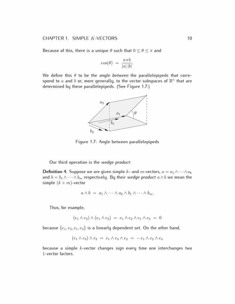
Because of this, there is a unique θ such that 0 ≤ θ ≤ π and

cos(θ) =a • b

|a| |b| .

We define this θ to be the angle between the parallelepipeds that corre-spond to a and b or, more generally, to the vector subspaces of Rn that aredetermined by these parallelepipeds. (See Figure 1.7.)

a1

a2

θ

b1

b2

Figure 1.7: Angle between parallelepipeds

Our third operation is the wedge product :

Definition 4. Suppose we are given simple k- and m-vectors, a = a1∧· · ·∧akand b = b1 ∧ · · · ∧ bm respectively. By their wedge product a∧ b we mean thesimple (k +m)-vector

a ∧ b = a1 ∧ · · · ∧ ak ∧ b1 ∧ · · · ∧ bm.

Thus, for example,

(e1 ∧ e2) ∧ (e1 ∧ e3) = e1 ∧ e2 ∧ e1 ∧ e3 = 0

because {e1, e2, e1, e3} is a linearly dependent set. On the other hand,

(e1 ∧ e3) ∧ e2 = e1 ∧ e3 ∧ e2 = − e1 ∧ e2 ∧ e3

because a simple k-vector changes sign every time one interchanges two1-vector factors.

Chapter 2

The Space of k-Vectors

2.1 The vector space ΛkRn

We now permit ourselves to add simple k-vectors and call the results k-vectors. We write down formal sums; that is we put down expressions suchas 3 (e1 ∧ e2) + 1.5 (e1 ∧ e3) and act as though we know what we are doing.Simple k-vectors have a geometric interpretation as equivalence classes oforiented parallelepipeds, but sums of simple k-vectors often lack such aninterpretation. However one can do algebra with them, and this can makethem very useful.

A careful justification for this operation of addition can be found in [5]. Itis shown there that this can be done in such a way that we obtain a vectorspace which we designate ΛkRn, the space of k-vectors in Rn. That is, ΛkRn

is vector space in that it satisfies all the axioms of a vector space: If weassume a, b, c are k-vectors and λ and ξ are scalars, then

1. a+ (b+ c) = (a+ b) + c.

2. λ(a+ b) = λa+ λb.

3. (λξ)a = λ(ξa).

4. a+ 0 = a.

5. a+ b = b+ a.

6. 0 a = 0 and 1 a = a.

11

CHAPTER 2. THE SPACE OF K-VECTORS 12

7. a+ (−a) = 0.

Recall that −a is (−1)a, and we may take 0 to be the simple k-vector corre-sponding to a degenerate k-parallelepiped.

In the event that k > n, we take ΛkRn to be the vector space consistingof a single element, 0. The reason for this is that if we are given a simplek-vector a1 ∧ · · · ∧ ak where k > n, then {a1, . . . , ak} must be a linearlydependent set, and thus a1 ∧ · · · ∧ ak = 0.

We take Λ1Rn to just be Rn, and it is convenient to identify Λ0Rn withthe set of real numbers, R.

2.2 Wedge productWe want to consider the special features of ΛkRn.

The most outstanding of these is the existence of the wedge product : Inthe expression a1 ∧ · · · ∧ ak, the symbol ∧ is merely a part of our notation fora simple k-vector. However we do know that it is possible to form a wedgeproduct of simple k- and m-vectors to form a simple (k +m)-vector:

(a1 ∧ · · · ∧ ak) ∧ (b1 ∧ · · · ∧ bm) = a1 ∧ · · · ∧ ak ∧ b1 ∧ · · · ∧ bm.We can extend wedge as a binary operation to all k-vectors. Given a, b, cwhich are p-, q-, and r-vectors respectively and λ a scalar, we can constructthe wedge product to have the following properties:

1. a ∧ b is a (p+ q)-vector.

2. a ∧ (b ∧ c) = (a ∧ b) ∧ c.

3. λ(a ∧ b) = (λa) ∧ b = a ∧ (λb).

4. Assuming q = r,a ∧ (b+ c) = a ∧ b+ a ∧ c.

Assuming p = q,(a+ b) ∧ c = a ∧ c+ b ∧ c.

It turns out to be convenient to treat scalars as 0-vectors and to define thewedge product of a scalar λ and a k-vector thus:

λ ∧ a = a ∧ λ = λa.


Example 2. Using the properties listed above and the fact that interchangingthe order of vectors in a simple k-vector changes the sign of the simple k-vector, we “simplify" a wedge product in R4:

−3e2∧[(e1 ∧ e3) + 7(e3 ∧ e4)

]= − 3(e2 ∧ e1 ∧ e3)− 21(e2 ∧ e3 ∧ e4)= 3(e1 ∧ e2 ∧ e3)− 21(e2 ∧ e3 ∧ e4).

2.3 Bases for ΛkRn

The wedge product also has the following useful property: If {u1, . . . , un} isa basis for Rn, then the simple k-vectors of the form ui1 ∧ · · · ∧ uik wherei1 < · · · < ik constitute a basis for ΛkRn.

Example 3. We know that {e1, e2, e3} is a basis for R3, so bases for ΛkR3 areas indicated:

Λ2R3 : e1 ∧ e2, e1 ∧ e3, e2 ∧ e3.Λ3R3 : e1 ∧ e2 ∧ e3.

Notice that from the basis for Λ3R3, we see that dim(Λ3R3) = 1 and that ifa is any 3-vector in R3, it must have the form a = λ(e1 ∧ e2 ∧ e3) for somescalar λ.

Example 4. A basis for Λ2R4 is

e1 ∧ e2, e1 ∧ e3, e1 ∧ e4, e2 ∧ e3, e2 ∧ e4, e3 ∧ e4.

Thus dim(Λ2R4) = 6.

This last example is a particular case of the following:

Proposition 2. For k = 0, 1, . . . , n, the dimension of ΛkRn is the binomialcoefficient

(nk

).

This is because, starting with a basis {ui}ni=1 and forming basis k-vectorsui1 ∧ · · · ∧ uik where i1 < · · · < ik, we see that we are concerned to count the


number of sequences of length k, (i1, . . . , ik), that we can form by choosingfrom the set of n objects {1, . . . , n}.

This is perhaps a good place to introduce the idea of multi-indices. Amulti-index is the same thing as an index except that it may have severalentries. By a multi-index I of length k, we mean a sequence I = (i1, . . . , ik)where each ir comes from some set of indices. Sometimes we drop the paren-theses and write I = i1 . . . ik. Thus, for example, if we consider a matrix withentries αij , we can say that ij is a multi-index of length 2.

We will say that a multi-index I = (i1, . . . , ik) is ordered if i1 < · · · < ik.Let {ui}ni=1 be a basis for Rn and let us form a multi-index I = (i1, . . . , ik).then we set

uIdef.= ui1 ∧ · · · ∧ uik .

By our remarks about bases for ΛkRn, we see that every k-vector a has aunique expansion

a =∑I

λIuI

where the summation is over all the multi-indices of length k that are orderedand the each λI is a scalar.

2.4 Reversion and dot productWe can also apply the operation of reversion and take dot products of k-vectors.

Recall that the reversion of a simple k-vector is

(a1 ∧ · · · ∧ ak)† = ak ∧ · · · ∧ a1,

that is, we just reverse the order of the factors. We also know that ai ∧ aj =−aj ∧ ai. If we permute the factors of a1 ∧ · · · ∧ ak one at a time to obtain thereversion ak ∧ · · · ∧ a1, then we find that

(a1 ∧ · · · ∧ ak)† = (−1)ra1 ∧ · · · ∧ ak where r =k(k − 1)

2.

We can define reversion for an arbitrary k-vector by extending the definitionon simple k-vectors linearly. That is, we know that any k-vector a can be


expanded into a linear combination of simple k-vectors, a =∑

I λIaI whereeach aI is simple. Then

a† =∑I

λIa†I .

An equivalent description is

a† = (−1)r∑I

λIaI where r =k(k − 1)

2.

In same way, we extend the definition of dot product linearly from simplek-vectors to arbitrary k-vectors.

That is, we know that for simple k-vectors, we have

(a1 ∧ · · · ∧ ak) • (b1 ∧ · · · ∧ bk)† = det

a1 • b1 · · · a1 • bk...

ak • bk · · · ak • bk

.

If we have arbitrary k-vectors a =∑

I λIaI and b =∑

J ξJbJ where λI , ξJ arescalars and aI , bJ are simple k-vectors, then we take the dot product of a andb to be

a • b† =(∑

I

λIaI

)•

(∑J

ξJb†J

)=∑I

∑J

λIξJ(aI • b†J).

We now discover a nice game we can play with dot products if we havean orthonormal basis.

Let {ui}ni=1 be an orthonormal basis for Rn. We form the correspondingbasis k-vectors uI for ΛkRn where I ranges over all ordered multi-indices oflength k. We find that if i1 < · · · < ik and j1 < · · · < jk, then(

ui1 ∧ · · · ∧ uik)

•

(uj1 ∧ · · · ∧ ujk

)†=

{1 if (i1, . . . , ik) = (j1, . . . , jk),

0 if (i1, . . . , ik) 6= (j1, . . . , jk).


That is, {uI}I , for suitable I , acts as an “orthonormal” basis for ΛkRn. (Thereader is invited to check this calculation for k = 2.) To put it slightlydifferently, if we use ordered multi-indices of length k, we have

uI •uJ =

{1 if I = J,

0 if I 6= J.

The following result is then a trivial calculation:

Proposition 3. Suppose {ui}ni=1 is an orthonormal basis for Rn. Let a, b ∈ΛkRn and let us expand them thus:

a =∑I

λIuI , b =∑J

ξJuJ

where λI , ξJ are scalars and the sums are over all ordered multi-indices I, Jof length k. Then

1. a • a† =∑

I λ2I .

2. a • b† =∑

I λIξI .

This proposition says that ΛkRn is isomorphic to Rm (where m =(nk

))

not only in terms of vector space properties but also with respect to the dotproduct. We take advantage of this “isomorphism” to define the magnitude ofa k-vector a by the equation

|a| def.=√a • a†.

We also find that the Cauchy-Schwarz inequality holds for k-vectors:

|a • b| ≤ |a| |b|.

Provided a, b 6= 0, we can use this to define an “angle” θ between a and b by

cos(θ)def.=

a • b

|a| |b|

where 0 ≤ θ ≤ π. (We mentioned this previously for simple k-vectors.)

Chapter 3

Calculus With k-Vectors

We want to show some things one can do with k-vectors and calculus. How-ever we start with a simple but useful application in analytic geometry.

3.1 HyperplanesA line L in the plane or 3-dimensional space or more generally Rn is de-termined by two points. Let us call the points a0 and a1; we can also thinkof them as being vectors in Rn. (Figure 3.1.) Notice that a point x is on L

a0

a1

L

Origin

x

Figure 3.1: A line determined by two points

precisely when the vectors a1− a0 and x− a0 are linearly dependent, that is,when

(x− a0) ∧ (a1 − a0) = 0.

17

CHAPTER 3. CALCULUS WITH K-VECTORS 18

In other words, this last equation can be considered an equation for the line.(It is a nonparametric equation; no parameters have been introduced to helpus describe L.) Another way to specify L is give a point that it passes through(for example, a0) and a vector parallel to the line (for example, b = a1 − a0.)Then the equation for L becomes

(x− a0) ∧ b = 0. (3.1)

Example 5. Let L be the line in R3 passing through a0 = (1, 1, 2) = e1 + e2 +2e3 in the direction given by the vector b = 3e1 − e3. The arbitrary point xon L is represented as x = (χ1, χ2, χ3) = χ1e1 + χ2e2 + χ3e3. Then Equation(3.1) becomes[

(χ1 − 1)e1 + (χ2 − 1)e2 + (χ3 − 2)e3]∧ (3e1 − e3) = 0.

Multiplying out, this reduces to

−3(χ2 − 1) e1 ∧ e2 + (−χ1 − 3χ2 + 7) e1 ∧ e3+(−χ2 + 1) e2 ∧ e3 = 0.

Since e1 ∧ e2, e1 ∧ e3, and e2 ∧ e3 constitute a basis for Λ2R3, the coefficientsof the last equation must be zero, and Equation (3.1) ultimately reduces tothe two scalar equations

χ1 + 3χ3 = 7,

χ2 = 1

which specify L.

Equation (3.1) can be generalized to describe any k-dimensional hyper-plane in Rn.

To say that H is a k-dimensional hyperplane means that it must be atranslate of a k-dimensional vector subspace of Rn. To be more specific, letV be a k-dimensional vector subspace of Rn. Next choose a point a0 in Rn.If we want a hyperplane passing through a0, we can translate V to a0. Wedo this by replacing every point x of V by x + a0 and calling the resultantset a0 + V ; this is our hyperplane H .

Now since V is a vector subspace and k-dimensional, we can find a basisa1, . . . , ak for V . These vectors will still be “parallel” to a0 + V . Then an


arbitrary point x in Rn will belong to our hyperplane if and only if the vectorx− a0 is a linear combination of a1, . . . , ak; that is, if and only if the vectorsx − a0, a1, . . . , ak are linearly dependent. This condition is captured by theequation

(x− a0) ∧ (a1 ∧ · · · ∧ ak) = 0. (3.2)

3.2 DifferentiabilityWe want to move beyond hyperplanes to more general surfaces. It is desirableto first indicate what we mean by differentiability.

If φ is a real-valued function with domain in Rn, we say that φ is C1 atx0 = (χ01, . . . , χ0n) in the domain of φ provided each of the partial derivatives∂φ/∂χi exists and is continuous in some open neighborhood of x0. We saythat φ is Ck at x0 provided each of the mixed partials

∂kφ

∂χi1 · · · ∂χikexists and is continuous in some open neighborhood of x0.

One of the most useful results of being Ck is that the order in which thedifferentiations are performed is irrelevant. Thus if φ is a function of χ and ξand is C2, we have

∂2φ

∂χ ∂ξ=

∂2φ

∂ξ ∂χ.

We generalize the previous discussion in two ways: Suppose first of allthat f is a vector-valued function with domain in Rn. We mean here thatf takes on values in Rn or some other Rm; this generalizes the idea of areal-valued function. Second, instead of considering partial derivatives of f ,we consider directional derivatives. We say that the directional derivative off at x0 in the direction specified by the vector v is

∂vf(x0)def.= lim

λ→0

1

λ

[f(x0 + λv)− f(x0)

](3.3)

where it is understood that λ is a scalar. If f is a function of the realvariables χ1, . . . , χn, that is, we have f(χ1, . . . , χn), then we get back to


partial derivatives via the notation

∂f

∂χi

def.= ∂eif.

If f : U → Rn where U is an open subset of some Rm, we say that f isdifferentiable at x0 ∈ U if there is a linear transformation f ′(x0) : Rm → Rn

and a function g : V → Rn where V is a neighborhood of 0 in Rm such that

f(x0 + v)− f(x0) =[f ′(x0)

]v + g(v) for v ∈ V

andlimv→0

g(v)

|v| = 0.

f is differentiable on U if it is differentiable at every x ∈ U . We call the mapv 7→

[f ′(x0)

]v the differential of f .

When we look at this definition, we see that

1

λ

[f(x0 + λv)− f(x0)

]=[f ′(x0)

]v +

g(λv)

λ.

Thus if we let λ→ 0, we have[f ′(x0)

]v = lim

λ→0

1

λ

[f(x0 + λv)− f(x0)

]= ∂vf(x0).

Here is a standard result from analysis:

Proposition 4. If f is C1 on the open set U , then it is differentiable at everypoint of U .

3.3 Surfaces and tangent vectorsBy a surface, we mean something like a surface of the type one encountersin introductory calculus or analytic geometry or, a little more generally a“manifold-with-corners." A hyperplane is an example of what we have in mind.We shall not give a precise definition of “surface” but shall say enough aboutthe idea we have in mind that we can work with it.


The important thing about p-dimensional surfaces is that one can coverthem with what we will call coordinate patches or local parametrizations, andthese parametrizations are assumed to have certain nice properties.

If x0 is a point in M, we want to be able to find an open subset U of Rp

and a map x : U →M such that

1. x0 ∈ x(U).

2. x is one-to-one.

We say that x or x(U) (we are not very careful about the distinction) is acoordinate patch containing x0. We also say that x is a local parametrizationof M. Suppose the coordinates of a point t ∈ Rp are (τ1, . . . , τp). If, underour coordinate patch x, we have x0 = x(t0) and t0 = (τ01, . . . , τ0p), then wesay that x0 has the coordinates (τ01, . . . , τ0p) with respect to this coordinatepatch or parametrization.

If we want to say that M is Cr surface (where r ≥ 1), we require that foreach coordinate patch x, the maps x and x−1 be Cr.

Now a little notation. Since we are letting (τ1, . . . , τp) be the coordinatesof t ∈ dom(x) ⊆ Rp, let us introduce the notation

∂x

∂τi

def.= ∂eix.

(We are, of course, assuming that x is at least C1.) The way we have donethis, ∂x/∂τi should be a function of t0 ∈ Rp, but sometimes we shall abusenotation and write it as a function of x0 ∈ M. Since x is a one-to-one map,we should not get into trouble.

Now here is an important point: Each ∂x/∂τi, when evaluated at x0 (ort0), is a tangent vector to M at the point x0.

We may define a tangent vector to M thus:

tangent vector to M at x0

= λ1

( ∂x∂τ1

(x0))

+ · · ·λp( ∂x∂τp

(x0)) (3.4)

where λ1, . . . , λp are scalars. That is, it is a linear combination of the tangentvectors ∂x/∂τi when evaluated at x0. (Of course, this definition does notdepend on which parametrization x we use.) By Tx0M we shall mean thespace of all tangent vectors to M at x0.


A second and sometimes useful way to construct a tangent vector to M

at x0 is this: Let f : U → M be a map where U is a subset of R; in otherwords, f defines a curve in M. We assume f passes through x0; without lossof generality, we suppose that f(0) = x0. Assuming further that f is at leasta C1 function, if

v = limλ→0

1

λ

[f(λ)− f(0)

]= f ′(0),

then v is a tangent vector to M at x0. This method of constructing tangentvectors to a surface is equivalent to the characterization of (3.4).

There is one other property we shall require of coordinate patches, some-thing we call nonsingularity: At every x0 in the coordinate patch x, if x0 =x(t0), then we require that the vectors ∂e1x(t0), . . . , ∂epx(t0) be linearly in-dependent. Then the requirement that the parametrization x be nonsingularamounts to

∂x

∂τ1(x0) ∧ · · · ∧

∂x

∂τp(x0) 6= 0.

If M were a one-dimensional curve and x was the path of a particle tracingthe curve, then this condition would amount to saying that the particle neverstops moving. More generally, we are requiring that at every point of M,we have a tangent p-parallelepiped (∂x/∂τ1) ∧ · · · ∧ (∂x/∂τp) with positivep-volume. Another way to think of this is that the parametrization x maps“small” regions of positive p-volume in Rp to “small” tangent sets also ofpositive p-volume.

A particularly useful surface is the cell. This is because other surfacescan be thought of as being composed of cells that are joined together “nicely.”

In what follows, by I we mean the unit interval [0, 1]. By the k-dimensionalunit cube Ik we mean I× · · · × I with k factors.

Definition 5. We say that M is a Cr p-cell (contained in some Rn) providedthere exists a Cr coordinatization (or parametrization) x : Ip →M such that

1. x : Ip →M is one-to-one and onto.

2. x and x−1 are Cr.

3. ∂x∂τ1∧ · · · ∧ ∂x

∂τp6= 0 everywhere on M.

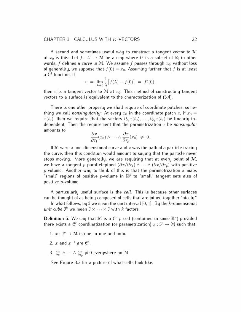
See Figure 3.2 for a picture of what cells look like.


Figure 3.2: 2-cell and 3-cell

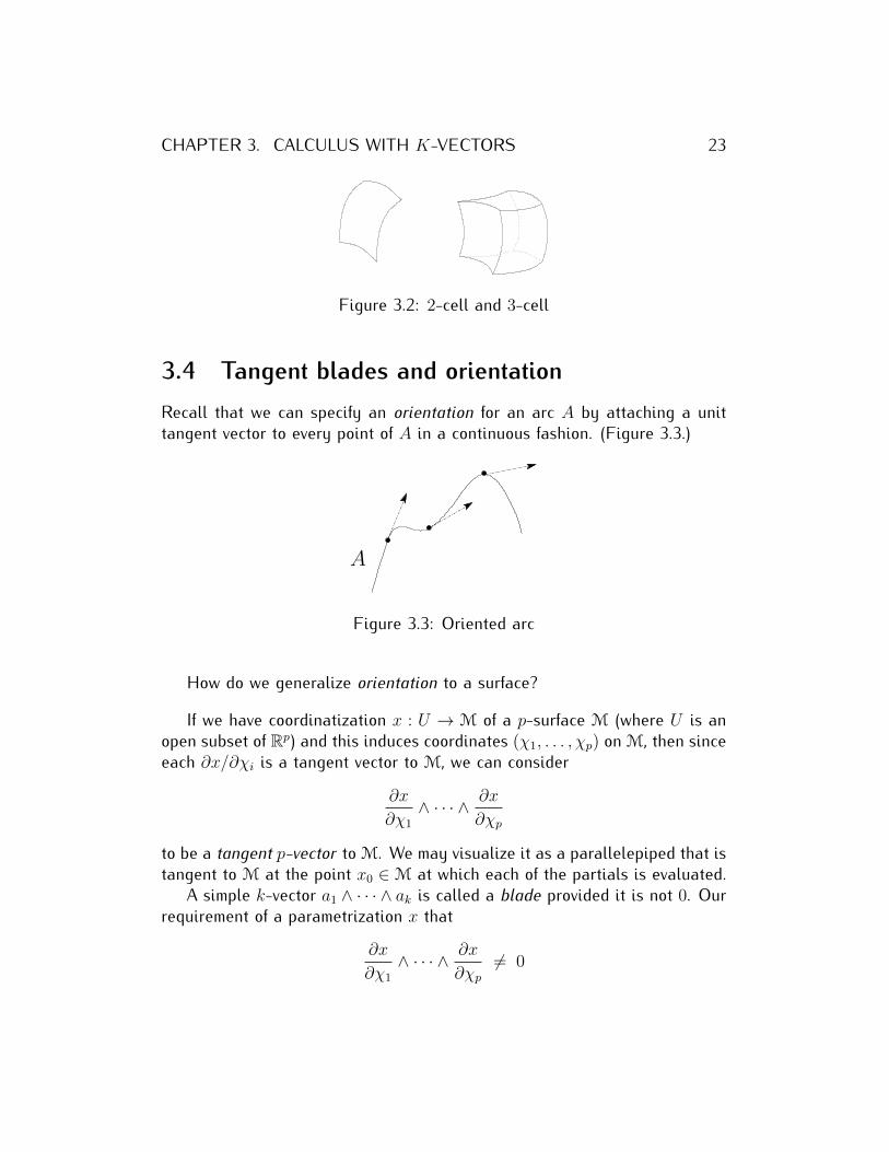
3.4 Tangent blades and orientationRecall that we can specify an orientation for an arc A by attaching a unittangent vector to every point of A in a continuous fashion. (Figure 3.3.)

A

Figure 3.3: Oriented arc

How do we generalize orientation to a surface?

If we have coordinatization x : U → M of a p-surface M (where U is anopen subset of Rp) and this induces coordinates (χ1, . . . , χp) on M, then sinceeach ∂x/∂χi is a tangent vector to M, we can consider

∂x

∂χ1

∧ · · · ∧ ∂x

∂χp

to be a tangent p-vector to M. We may visualize it as a parallelepiped that istangent to M at the point x0 ∈M at which each of the partials is evaluated.

A simple k-vector a1 ∧ · · · ∧ ak is called a blade provided it is not 0. Ourrequirement of a parametrization x that

∂x

∂χ1

∧ · · · ∧ ∂x

∂χp6= 0


then amounts to the claim that this tangent parallelepiped is a p-blade.By an orientation of the p-surface M, we mean a continuous function w

that assigns to every point x of M a unit tangent blade w(x). That is, w(x)must have the form a1 ∧ · · · ∧ ap where each ai is a tangent vector to M at xand |w(x)| = 1.

Example 6. By the standard orientation of Rn we mean the constant n-bladee1 · · · en = e1 ∧ · · · ∧ en.

Every C1 surface M has local orientations around every point x0 ∈ M.That is, a unit tangent blade w(x) can be assigned continuously to someneighborhood of x0 in M. If the orientation can be extended to all of M, thesurface is orientable; otherwise, as in the case of a Möbius strip, the surfaceis nonorientable.

A connected, orientable surface M has precisely two orientations. If oneof them is w, the other is −w.

If w is an orientation of the p-surface M and x is a parametrization of M,we say that x agrees with the orientation of M provided

w =

∂x∂χ1∧ · · · ∧ ∂x

∂χp∣∣∣ ∂x∂χ1∧ · · · ∧ ∂x

∂χp

∣∣∣ .3.5 IntegralsWe start with the change-of-variables formula for integrals:

Suppose U and V are open subsets of Rn and x : U → V is a one-to-oneonto map such that both x and x−1 are C1. If φ : V → R and φ is integrableover V , then (φ ◦ x) | det x ′| is integrable over U and∫

U

(φ ◦ x) | det x ′| =∫V

φ. (3.5)

(See [4] or [10] for a proof.) The expression | det x ′| is a kind of “local mag-nification factor” for the way the map x changes n-dimensional volume atany given point. The expression det x ′ may be familiar to the reader as theJacobian determinant.

Using the wedge product, this formula can be generalized to define whatwe mean by an integral over a k-dimensional surface M in Rn.


Suppose that x : U → M is a parametrization of M and it assigns co-ordinates (τ1, . . . , τk) to points of M. Recall this means that a point p ∈ M

has coordinates (τ1, . . . , τk) with respect to the parametrization (or coordinatepatch) x if p = x(τ1, . . . , τk). We intend U to be a “nice” subset of Rk, forexample, a k-cell, rectangle, simplex, open set, etc. We set∫

M

φdef.=

∫U

(φ ◦ x)∣∣∣ ∂x∂τ1∧ · · · ∧ ∂x

∂τk

∣∣∣. (3.6)

The integral on the right is that of a real-valued function over a “nice” subsetof Rk, so we expect it to be integrable using standard techniques of calculus.

We know that∂x

∂τ1∧ · · · ∧ ∂x

∂τk

can be envisioned as an oriented k-dimensional parallelepiped that is tangentto M, and ∣∣∣ ∂x

∂τ1∧ · · · ∧ ∂x

∂τk

∣∣∣is the k-volume of that parallelepiped. In the case where k = n, then∣∣∣ ∂x

∂τ1∧ · · · ∧ ∂x

∂τk

∣∣∣ = | det(x ′)|,

and we are back to the change-of-variables formula.

Example 7. Let S1 be the unit circle in R2. We will take M to be S1×S1. Thisis a torus in R4 and satisfies the two equations χ2

1 +χ22 = 1 and χ2

3 +χ24 = 1.

We know the length of S1 is 2π. Since M is a cartesian product with the twocopies of S1 lying in orthogonal spaces, it seems reasonable to guess thatthe area of M (the 2-dimensional volume) should be a product of lengths,(2π)2 = 4π2. At the same time, one would expect the 2-volume of M to begiven by

∫M

1. Do the two intuitions agree? Let us figure out how to evaluatethe integral.

We know that we can parametrize S1 thus:

θ 7→ cos(θ) e1 + sin(θ) e2.

So we take

x(ψ, ξ) = cos(ψ) e1 + sin(ψ) e2 + cos(ξ) e3 + sin(ξ) e4,


where (ψ, ξ) ∈ [0, 2π]× [0, 2π], as our parametrization of M.(There is a slight technical difficulty here since this parametrization is not

one-to-one on the edges of the square. However the problem occurs on a“small set,” one that is of “measure zero,” and it can be shown that this doesnot influence the answer.)

We see that∂x

∂ψ= − sin(ψ) e1 + cos(ψ) e2,

∂x

∂ξ= − sin(ξ) e3 + cos(ξ) e4,

and we readily calculate that ∣∣∣ ∂x∂ψ∧ ∂x∂ξ

∣∣∣ = 1.

We finally evaluate the integral:∫M

1 =

∫[0,2π]2

∣∣∣ ∂x∂ψ∧ ∂x∂ξ

∣∣∣=

∫ 2π

0

∫ 2π

0

1 dψ dξ = 4π2.

We can replace φ in the integral of (3.6) by a p-vector field f . We needonly start with the standard basis {ei}ni=1 for Rn and write f in terms of it:

f =∑|I|=p

φIeI

where it is understood that I ranges over all multi-indices which are bothordered and of length p and each φI is a real-valued function. f always hassuch a decomposition, and it is unique. We then set∫

M

fdef.=∑|I|=p

(∫M

φI

)eI . (3.7)

Of course {ei}ni=1 can be replaced by any basis {ui}ni=1 for Rn provided thebasis elements are constant vectors. We call (3.6) and (3.7) unoriented inte-grals.


We know that in elementary, single-variable calculus, we deal with ori-ented integrals. We can see this from the fact that given a real-valued functionof a single variable, φ(τ), we have∫ β

α

φ(τ) dτ = −∫ α

β

φ(τ) dτ.

That is, orientation is taken account of by noting the direction in which weintegrate.

We shall see later how to generalize the notion of oriented integral tosurfaces. It is convenient to first develop the ideas of the geomtric productand geometric algebra.

Chapter 4

Geometric Algebra

4.1 Gn and gradesWe now construct the geometric algebra over Rn and denote it Gn. This is avector space that contains and is generated by R, Rn, Λ2Rn, . . . , ΛnRn. In Gn

it is perfectly legal to add k-vectors which have different values of k. Thuswe get to write expressions such as

√2− 7 e1 ∧ e3. It follows that in G3, for

example, every element will be of the form α + a + b + c where α is a realnumber, a is a vector, b is a 2-vector, and c is a 3-vector. We call the elementsof Gn multivectors.

We can write Gn as a direct sum of the different spaces of k-vectors inRn:

Gn = R⊕ Rn ⊕ Λ2Rn ⊕ · · · ⊕ ΛnRn.

Of course, we feel free to write R = Λ0Rn and Rn = Λ1Rn. If a multivector isa sum of k-vectors, then we say it is of grade k. Thus 4 e1 ∧ e2−π e2 ∧ e3 is agrade 2 multivector. On the other hand,

√2− 7 e1 ∧ e3 cannot be assigned a

unique grade because it is the sum of a grade 0 and a grade 2 term. If a is amultivector, we use the symbol

⟨a⟩k

for the sum of the grade k terms that occurin it. Thus for every multivector a in Gn we have a unique decomposition:

a =⟨a⟩0

+⟨a⟩1

+ · · ·⟨a⟩n.

If we take a =√

2− 7 e1 ∧ e3, an element of G3, then for this multivector,⟨a⟩0

=√

2,⟨a⟩1

= 0,

28

CHAPTER 4. GEOMETRIC ALGEBRA 29⟨a⟩2

= −7 e1 ∧ e3,⟨a⟩3

= 0.

4.2 The geometric productIn spaces of k-vectors, we are familiar with the operations of multiplication byscalars, addition, the dot product, and the wedge product. These operationscan be extended into Gn. And we add one more operation, the geometricproduct, which can be thought of as a generalization of both the dot and thewedge products.

We write the geometric product of multivectors a and b as ab. This isnot, in general, commutative. Careful constructions of it are given in [7] and[12]. Here we follow an exposition reminiscent of [6] and simply describe theproperties of the geometric product.

Properties of the geometric product

1. If a, b, c ∈ Gn and λ ∈ R, then

(a) 1 a = a 1 = a.(b) a (b+ c) = ab+ ac and (a+ b) c = ac+ bc.(c) λ (ab) = (λa) b = a (λb).(d) a(bc) = (ab)c.

2. If a, b ∈ Rn, thenab = a • b+ a ∧ b.

3. If u1, . . . , up are orthogonal vectors, then

u1 · · ·up = u1 ∧ · · · ∧ up.

Notice that it is properties 2 and 3 that exhibit the connection betweenthe geometric, dot, and wedge products.

An immediate consequence of property 2 is that if a is a vector of Rn, thenaa = |a|2. This is because a • a = |a|2 and a ∧ a = 0.

CHAPTER 4. GEOMETRIC ALGEBRA 30

If we wish to calculate a geometric product, it is often helpful to express ourmultivectors in terms of an orthonormal basis for Rn. Suppose, for example,that u1, u2, u3 are orthonormal vectors. Then

u1(u1u2) = u2 (because |u1|2 = 1),u2(u1u3) = u2 ∧ u1 ∧ u3 = −u1 ∧ u2 ∧ u3 = −u1u2u3.

We can show the following:

Proposition 5. If {ui}ni=1 is a basis for Rn, then the set consisting of 1 and theblades ui1 ∧ · · · ∧ uik such that i1 < · · · < ik and k = 0, 1, . . . , n constitutes abasis for Gn.

Thus a basis for G3 is

1, e1, e2, e3, e1e2, e1e3, e2e3, e1e2e3.

Keep in mind when we say this, that a basis element such as e1e2 is the samething as e1 ∧ e2 because e1 and e2 are orthogonal. So we can also say thata basis for G3 is

1, e1, e2, e3, e1 ∧ e2, e1 ∧ e3, e2 ∧ e3, e1 ∧ e2 ∧ e3.

Corollary 1. The dimension of Gn is 2n.

This is seen from the fact that the dimension of ΛkRn is(nk

)and(

n

0

)+

(n

1

)+ · · ·+

(n

n

)= 2n.

4.3 Extending reversionOne of our concerns is to extend operations defined for k-vectors to arbitrarymultivectors. (Remember, not all multivectors are k-vectors. An example is√

2− 7 e1e3. We want our extended operations to work in this larger space.)The first of these is reversion:

If u1, . . . , uk are orthogonal vectors, then we see that

(u1 · · ·uk)† = (u1 ∧ · · · ∧ uk)†= uk ∧ · · · ∧ u1


= (−1)k(k−1)

2 u1 ∧ · · · ∧ uk= (−1)

k(k−1)2 u1 · · ·uk.

We can do this because we know how to take the reversion of a k-vector. Weknow that a multivector in Rn has a unique expansion into k-vectors thus:

a =⟨a⟩0

+⟨a⟩1

+ · · ·+⟨a⟩n.

We define the reversion of a multivector in this way:

a†def.=

n∑k=0

(−1)k(k−1)

2

⟨a⟩k.

One can, of course, show that reversion is linear (that is, (λa)† = λa† and(a+ b)† = a† + b†) and that (ab)† = b†a†.

4.4 The scalar productThe second operation we extend from k-vectors to multivectors is the dotproduct. There is definitely more than one useful way to do this; four of themare considered in [12]. We exhibit only one, the scalar product.

Definition 6. If a and b are multivectors in Rn, that is, a, b ∈ Gn, then theirscalar product is

⟨ab†⟩0.

This product is commutative, and it does not matter which factor gets thedagger: ⟨

ab†⟩0

=⟨a†b⟩0

=⟨ba†⟩0

=⟨b†a⟩0.

It is easily seen that the scalar product generalizes the dot product ofvectors: Suppose that a, b ∈ Rn; that is, a and b are grade 1. Note thatb† = b trivially. We know that ab = a • b+ a ∧ b. We see that a • b is grade 0while a ∧ b is grade 2. Thus⟨

ab†⟩0

=⟨ab⟩0

=⟨a • b+ a ∧ b

⟩0

= a • b.

It can also be shown that if a and b are simple k-vectors, a = a1 ∧ · · · ∧ akand b = b1 ∧ · · · ∧ bk, then⟨

ab†⟩0

= det(ai • bj)k×k,


the determinant of a k × k matrix, so that the scalar product generalizes thedot product of k-vectors.

The scalar product looks particularly nice if one writes everything in termsof an orthonormal basis:

Let {ui}ni=1 be an orthonormal basis for Rn. We know that {uI}I , whereI runs through all ordered multi-indices, is a basis for Gn. We see that

⟨uIu

†J

⟩0

=

{1 if I = J,

0 if I 6= J.

This follows from the fact that if uI is a p-vector and uJ is a q-vector withp 6= q, then the product uIu†J cannot be grade 0. While if p = q, then thescalar product reduces to the dot product of p-vectors. In any event, we cantreat {uI}I as an “orthonormal” basis for Gn.

Next let a and b be multivectors in Rn and write their unique expansionsin terms of {uI}I :

a =∑I

αIuI and b =∑I

βIuI .

Then we have ⟨aa†⟩0

=∑I

α2I ,⟨

ab†⟩0

=∑I

αIβJ .

We define the magnitude of the multivector a thus:

|a| def.=√⟨

aa†⟩0.

Notice that we are simply echoing things we said earlier about k-vectors inSection 2.4 and Proposition 3 but now on the broader stage of Gn.

4.5 The wedge product of multivectorsThe easiest operation to extend to multivectors is the wedge product. Thequick-and-dirty way to do it is to assume that this extended operation hasthe following, obviously desirable properties:

If a, b, c are multivectors in Rn and λ is scalar, then the following hold:


1. a ∧ (b+ c) = (a ∧ b) + (a ∧ c).

2. (a+ b) ∧ c = (a ∧ c) + (b ∧ c).

3. λ(a ∧ b) = (λa) ∧ b = a ∧ (λb).

4. λ ∧ a = a ∧ λ = λa.

5. (a ∧ b)† = b† ∧ a†.This permits us to reduce all wedge products of multivectors to wedge productsof simple p- and q-vectors which we already (presumably) know how to do.Thus, for example,

(2 + 3 e1e4) ∧ (1− e1 + e2) = 2− 2e1 + 2e2

+ 3 e1e4 − 3 (e1e4) ∧ e1 + 3 (e1e4) ∧ e2= 2− 2e1 + 2e2 + 3 e1e4 − 3e1e2e4.

(Notice in this calculation that

(e1e4) ∧ e1 = e1 ∧ e4 ∧ e1 = 0,

(e1e4) ∧ e2 = e1 ∧ e4 ∧ e2 = −e1 ∧ e2 ∧ e4because the vectors are orthogonal.)

Of course, to simply assume the properties we want is cheating. It caneasily lead to disaster (as in, “Let us assume the following circle has threecorners . . . ”). To do this properly, we ought to provide a mathematical proofthat the extension can be carried out. We do not do this here, but one wayto do it is to use the following odd-looking definition of the extended wedgeproduct:

a ∧ b def.=

n∑p,q=0

⟨⟨a⟩p

⟨b⟩q

⟩p+q

.

(Details provided in [12].)

4.6 Division by multivectorsA very useful property of geometric algebra is that one can always divide byblades; in particular, one can divide by nonzero vectors. This something onecannot do in vector analysis.


Suppose that a is a k-blade in Rn. We know that a 6= 0 so |a| > 0. Noticethat since aa† = a†a = |a|2, we have

aa†

|a|2 =a†

|a|2 a = 1.

This amounts to saying that

a−1 =a†

|a|2 .

A case worthy of note is when we have a unit blade, as, for example, anorientation w of a surface. Then

w−1 = w† because |w| = 1.

Though blades always have inverses (with respect to the geometric prod-uct), there are nonzero multivectors that do not. Division is only possiblesome of the time.

Division often has an important geometric interpretation. To see this, leta be a k-blade in Rn and let e = e1 · · · en where {ei}ni=1 is the standard basis.We know that e is the standard orientation of Rn. It is always possible to findan orthonormal basis {ui}ni=1 of Rn such that a = λu1 · · ·uk where λ = |a|.We know that u = u1 · · ·un must also be an orientation for Rn, and since aconnected, n-dimensional surface (of which Rn is an example) can have onlytwo orientations, either u = e or u = −e. Let us assume, for the same ofsimplicity, that u = e. Then

ea−1 =1

λ(u1 · · ·un)(u1 · · ·uk)†

=(−1)r

λ(uk · · ·u1)(u1 · · ·un)

=(−1)r

λ(uk+1 · · ·un)

for some integer r. Now (−1)r(1/λ)(uk+1 · · ·un) is clearly orthogonal toa = λ(u1 · · ·uk). So what we have shown is that if you divide the orientationof Rn by a k-blade a, the result must be an (n− k)-blade that is orthogonalto a.


4.7 Reciprocal vectorsGiven a set of linearly independent vectors {ai}ki=1, a very useful trick wecan play with the geometric algebra is to construct the reciprocal set {bi}ki=1.(We shall demonstrate the usefulness in the next chapter.) The set {bi}ki=1 isunique and is defined by the properties

{ai}ki=1 and {bi}ki=1 span the same subspace, and

ai • bj =

{1 if i = j,

0 if i 6= j.

Here is a formula for computing bj from {ai}ki=1: Set a = a1 ∧ · · · ∧ ak. Then

bj = (−1)i−1(a1 ∧ · · · ∧ ai ∧ · · · ∧ ak)a−1

= (−1)k−ia−1(a1 ∧ · · · ∧ ai ∧ · · · ∧ ak),

where ai means that ai is omitted in this product. Notice that in this formula,we are taking the geometric product of a−1 and a1 ∧ · · · ∧ ai ∧ · · · ∧ ak.

Example 8. Let V be the subspace χ2 = χ3 of R3. A basis is a1 = e1 anda2 = e2 + e3. We readily compute that

a = a1 ∧ a2 = e1e2 + e1e3,

a−1 = −1

2(e1e2 + e1e3),

b1 = a2a−1 = e1,

b2 = −a1a−1 =1

2(e2 + e3).

If {ai}ki=1 is a basis for a subspace V , we naturally call {bi}ki=1 the recip-rocal basis. An independent set of vectors {ai}ki=1 is often called a frame. Inthat case, {bi}ki=1 is called the reciprocal frame.

Chapter 5

Derivatives and the FundamentalTheorem

5.1 Directional derivativesWe assume that M is p-dimensional C1 surface in Rm.

Suppose that f is a multivector field on M; that is, f : M → Gm. Weextend our definition of directional derivative to f :

∂uf(x0)def.= lim

λ→0

1

λ

(f(x0 + λu)− f(x0)

)where x0 is a point in M, u is a vector in Rm, and, of course, λ is a scalar.Provided f is “nice,” for example, if it is C1, then given x0, there is a lineartransformation f ′(x0) : Rm → Gm such that

∂uf(x0) =[f ′(x0)

](u).

The map u 7→[f ′(x0)

](u) as the differential of f at x0. If we have two maps

f and g and can form their composite, then we have the formula

∂u(f ◦ g

)(x0) =

[(f ◦ g

) ′(x0)

](u) =

[f ′(g(x0)

)] [g ′(x0)

](u) (5.1)

which is, in effect, the chain rule of multivariable calculus. This is often helpfulfor establishing theoretical results.

Continuing with our multivector field f on M, suppose we also have aparametrization x : U → M which induces coordinates (χ1, . . . , χp) on M.

36

CHAPTER 5. DERIVATIVES AND THE FUNDAMENTAL THEOREM 37

Then at the point x0 ∈M we define

∂f

∂χi(x0)

def.= ∂ei

(f ◦ x

)(r0) =

[(f ◦ x

) ′(r0)

](ei)

where U is a suitable subset of Rp and r0 is the unique point in Rp such thatx(r0) = x0. Notice that we are treating ∂f/∂χi as a function defined on thesurface M; this works because x is a one-to-one function.

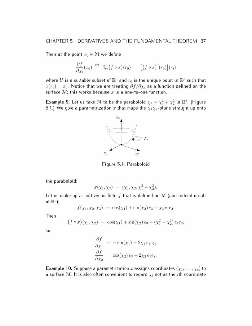
Example 9. Let us take M to be the paraboloid χ3 = χ21 + χ2

2 in R3. (Figure5.1.) We give a parametrization x that maps the χ1χ2-plane straight up onto

χ3

χ2χ1

M

Figure 5.1: Paraboloid

the paraboloid:x(χ1, χ2) = (χ1, χ2, χ

21 + χ2

2).

Let us make up a multivector field f that is defined on M (and indeed on allof R3):

f(χ1, χ2, χ3) = cos(χ1) + sin(χ2) e3 + χ3 e1e2.

Then (f ◦ x

)(χ1, χ2) = cos(χ1) + sin(χ2) e3 + (χ2

1 + χ22) e1e2,

so∂f

∂χ1

= − sin(χ1) + 2χ1 e1e2,

∂f

∂χ2

= cos(χ2) e3 + 2χ2 e1e2.

Example 10. Suppose a parametrization x assigns coordinates (χ1, . . . , χp) toa surface M. It is also often convenient to regard χi not as the ith coordinate


of a point but as a map χi : M → R that assigns to a point on M its ithcoordinate. That is, if x0 is a point on M and x(χ01, . . . , χ0p) = x0, thenχi(x0) = χ0i. This means that χi ◦ x = πi, the projection Rp → R that selectsthe ith entry of of a p-tuple. It then becomes easy to show that

∂χi∂χj

=

{1 if i = j,

0 if i 6= j.

It should not be surprising that the following version of the chain rule canbe established:Proposition 6. Let M be a C1 surface with two sets of coordinates, (χ1, . . . , χp)and (ξ1, . . . , ξp). If f is C1 multivector field on M, then

∂f

∂χi=

p∑j=1

∂f

∂ξj

∂ξj∂χi

.

5.2 The geometric derivativeLet M be a C1 p-surface in Rm. If x0 is a point in M and x is a parametrizationthat induces coordinates (χ1, . . . , χp) on M, then we know from Chapter 3 that{(∂x/∂χi

)(x0)}pi=1 is a basis for the tangent space Tx0M. We know there must

be a reciprocal basis; let us designate it {dχi(x0)}pi=1. Thus

∂x

∂χi• dχj =

{1 if i = j,

0 if i 6= j

at all points at which the two vector fields can be evaluated.We now come to the basic operation of geometric calculus.

Definition 7. If f is a multivector field on M, then→∇Mf

def.=

p∑i=1

∂f

∂χidχi,

←∇Mf

def.=

p∑i=1

dχi∂f

∂χi.

We call these the right-hand and left-hand geometric derivative respectivelydepending on the direction of the arrow.


(In the literature, one usually considers only←∇Mf , and it is called the

vector derivative; but we prefer the term geometric derivative.)It is important to note two things about this definition. First, the product

of the multivector field ∂f/∂χi and the vector dχi is the geometric product.In general,

∂f

∂χidχi 6= dχi

∂f

∂χi,

so the right-hand and left-hand geometric derivatives need not be equal. Thisis not a real difficulty since one can show that(→

∇Mf)†

=←∇M(f †).

The second important point is that the geometric derivative is independent ofthe choice of coordinates. Thus if (ξ1, . . . , ξp) is a second set of coordinateson M, we have

p∑i=1

∂f

∂χidχi =

p∑j=1

∂f

∂ξjdξj.

Example 11. Take M to be Rm and let the parametrization x be the identitymap, x(χ1, . . . , χp) = (χ1, . . . , χp). Then ∂x/∂χi = ei and dχi = ei. If φ is areal-valued function on Rm, then

→∇Mφ =

←∇Mφ =

m∑i=1

∂φ

∂χiei

which is simply the gradient of φ.

The following result should not be surprising:

Proposition 7. Suppose (χ1, . . . , χp) and (ξ1, . . . , ξp) are two sets of coordi-nates on the C1 surface M. Then

dχi =

p∑j=1

∂χi∂ξj

dξj.


5.3 Oriented integralsSuppose f is a multivector field defined over a surface M. If x : U → M

is a parametrization of M (where U ⊆ Rp) we know from Chapter 3 how tointegrate f over M:∫

M

f =

∫U

(f ◦ x)∣∣∣ ∂x∂χ1

∧ · · · ∧ ∂x

∂χp

∣∣∣. (5.2)

The last expression is evaluated using standard calculus-type techniques andwill produce a number or a multivector.

Suppose that M also has an orientation w. By an oriented integral of fover M we mean something of (approximately) the form∫

M

fw

where fw is the geometric product of f and w and the integral is evaluatedusing (5.2). This is a generalization of the oriented integral∫ β

α

φ(χ) dχ

of single-variable calculus. Since we are integrating along the interval [α, β]which is a set of real numbers, the only orientations are the real numbers +1or −1. In this setting,

∫Mfw amounts to∫

[α,β]

φ (+1) or∫[α,β]

φ (−1)

depending on whether we want∫ βαφ or

∫ αβφ.

There are a number of variations possible on the form∫Mfw, for example,∫

M

wf,

∫M

fw†,

∫M

f (−w), etc.

We will refer to them all as oriented integrals of f . Because of the complexitypossible with multivector fields, unlike real-valued single-variable integrals,these may reduce to more than just two values. The particular oriented inte-gral we want will depend on the problem we are trying to solve.

Here is a particularly useful example of an oriented integral:


Proposition 8. Suppose that the C1 surface M has a parametrization x : U →M which induces coordinates (χ1, . . . , χp). Suppose further that M has anorientation w that agrees with the parametrization in the sense that

w = λ( ∂x∂χ1

∧ · · · ∧ ∂x

∂χp

)where λ > 0. If f is the multivector field φ (dχ1 ∧ · · · ∧ dχp) where φ is areal-valued function on M, then∫

M

φ (dχ1 ∧ · · · ∧ dχp)w† =

∫U

(φ ◦ x

)(χ1, . . . , χp) dχ1 · · · dχp

where the last integral is an iterated integral, and each dχi is not a vectorbut instead indicates the variable with respect to which one is integrating.

Of course, in this proposition,

λ =1∣∣∣ ∂x∂χ1

∧ · · · ∧ ∂x∂χp

∣∣∣ .The integration formula is very straightforward to establish.

5.4 Induced orientationIn vector analysis, one may talk of using the unit outward normal vector tothe boundary of a region to define an orientation of that boundary. (Figure5.2.) In a higher dimensional setting, it is not clear one can define analogousconcepts. How, for example, would one do this for the boundary of a k-dimensional cell in Rn? Geometric algebra is very helpful here.

In general, if M is a p-cell in Rm with orientation w, we would expect anorientation ∂w of the boundary ∂M of the cell to be a unit tangent (p− 1)-blade which is continuous (except where one slips from one face to another ofthe cell). (Figure 5.3.) We assume here that p ≥ 2 and that M is at least C1.

Assume M is a cell with orientation w. It turns out that if one knowseither the unit outward normal vector n to the boundary ∂M at a given pointor the orientation of ∂M at that point, then one can define the other concept;further, this can be done in two different, useful ways.


boundary of R

outward normal ve tor

R

∂R

Figure 5.2: A region R with outward normal vector from the boundary

∂w

∂w ∂w

∂M

∂w

M

Figure 5.3: Cell with oriented boundary

The trick is that these quantities should satisfy the equations→∂w = nw and

←∂w = wn.

→∂w and

←∂w are, respectively, the right-hand and left-hand induced orienta-

tion on ∂M, and n is the unit outward normal vector to the boundary of M.In some dimensions, these two induced orientations coincide, and in others,they have opposite signs. They are connected by the equation(→

∂w)†

=←∂(w†).

Example 12. Let the unit square I2 in R2 have orientation w = e1e2. We seein Figure 5.4 that we should have n = e1 on the right side of ∂I2, n = −e1 on


n

n

n

n I2

Figure 5.4: Induced orientation on ∂I2

the left side, and so forth. For the right side of the boundary, since n = e1,we have

→∂w = e2. For the top side, since n = e2, we see that

→∂w = −e1. And

so forth. That is,→∂w amounts to giving ∂M the counterclockwise orientation.

When dealing with a p-cell M, one can start with an induced orientationon ∂Ip and use it to construct an induced orientation on ∂M.

Example 13. Suppose M is a 2-cell with a parametrization x : I2 →M. Let I2have the orientation e1e2, and the orientation of ∂I2 be the counterclockwiseone. (Figure 5.5.) We can transfer the orientation of I2 to an orientation w

x

e1

e2

−e1

MI2−e2

∂x∂χ2

− ∂x∂χ2

− ∂x∂χ1

∂x∂χ1

Figure 5.5: Transferring orientation from ∂I2 to ∂M

of M by the transformation

e1 ∧ e2 7→([x ′(r0)

]e1)∧([x ′(r0)

]e2)

=∂x

∂χ1

(x0) ∧∂x

∂χ2

(x0)


where x0 = x(r0). That is, we take w to be

w = λ( ∂x∂χ1

∧ ∂x

∂χ2

)where λ is a scalar chosen to make |w| = 1. In the same way, one can transferthe tangent 1-blades on ∂I2 to tangent 1-blades on ∂M via the transformation

ei 7→∂x

∂χi.

Thus, for example, on the right-hand edge of ∂M (see Figure 5.5), we willhave

→∂w = α

∂x

∂χ2

where α is a scalar chosen to normalize→∂w.

It is straightforward to generalize the discussion of this example to p-cells and show how to transfer an induced orientation on ∂Ip to an inducedorientation on ∂M.

5.5 The Fundamental TheoremWe now state—without proof—a version of the Fundamental Theorem of ge-ometric calculus:

Theorem 1. Let M be a C2 p-cell with orientation w. If f is a C1 multivectorfield on M, then ∫

∂M

f (→∂w) =

∫M

(→∇Mf

)w.

A second version has the same hypothesis and the equation∫∂M

(←∂w) f =

∫M

w(→∇Mf

)and readily follows from the fact that(∫

N

g)†

=

∫N

g†.

There is a third version involving two functions f and g on M, but we do notdiscuss it.


Example 14. The single variable form of the Fundamental Theorem from cal-culus can be viewed as a special case of Theorem 1: Let M be the interval[α, β] ⊆ R and f be a real-valued function φ on [α, β]. We take the orien-tation of [α, β] to be the real number 1. If we think of φ as a function of thecoordinate τ , then dτ = 1 because our tangent space at each point is R. Then∫

M

(→∇Mf

)w =

∫ β

α

φ ′.

The boundary of [α, β] is a two-point set, {α, β}. It is reasonable to regardthe induced orientation of the boundary of [α, β] as −1 at α and +1 at β andto interpret the “integral” over a two-point set as∫

∂M

f(→∂w)

= f(β)− f(α).

Thus Theorem 1 yields ∫ β

α

φ ′ = φ(β)− φ(α).

Example 15. Gauss’s divergence theorem in R3 is∫∂M

f •N =

∫M

div f

where f is a vector field, M is a bounded 3-dimensional region, and N is aunit vector directed outward from and orthogonal to the boundary. If we writef in the form f =

∑3i=1 φ ei, then

div f =3∑i=1

∂φi∂χi

.

This result is easily proved in generalized form in Rn using the FundamentalTheorem of geometric calculus.

Let M be a C2 n-cell in Rn, and let us give it the orientation w = e1 · · · en,the same as the standard orientation of Rn. If N is the unit outward normalvector to ∂M and

→∂w is the right-hand induced orientation on the boundary

of M, they will be related by the equation→∂w = N e1 · · · en. Now suppose


we have a vector field f on M and we write it in the form f =∑n

i=1 φiei. Wetake the divergence of the field to be

div f def.=

n∑i=1

∂φi∂χi

.

Next we write down the Fundamental Theorem as applied to these objects:∫∂M

f→∂w =

∫M

(→∇Mf

)w. (5.3)

We rewrite (5.3) as∫∂M

f N (e1 · · · en) =

∫M

(→∇Mf

)e1 · · · en,

and since e1 · · · en is a constant and in geometric algebra we can divide byblades, we reduce (5.3) to ∫

∂M

f N =

∫M

→∇Mf. (5.4)

We recall that if (χ1, . . . , χn) are just the coordinates of a point in Rn, thendχi = ei. Next we turn the crank and calculate that

→∇Mf =

n∑i=1

∂f

∂χiei = div f +

∑j<i

(∂φj∂χi− ∂φi∂χj

)ejei

where∑

j<i mean that we sum over all indices j and i such that j < i. Nownotice that since f and N are vectors, we have fN = f •N + f ∧ N . If wesubstitute back into (5.4), we obtain∫

∂M

f •N + f ∧N =

∫M

div f +∑j<i


)ejei. (5.5)

If we equate the integrals of grade 0 and grade 2 in (5.5), we obtain∫∂M

f •N =

∫M

div f and (5.6)∫∂M

f ∧N =∑j<i

∫M


)ejei. (5.7)


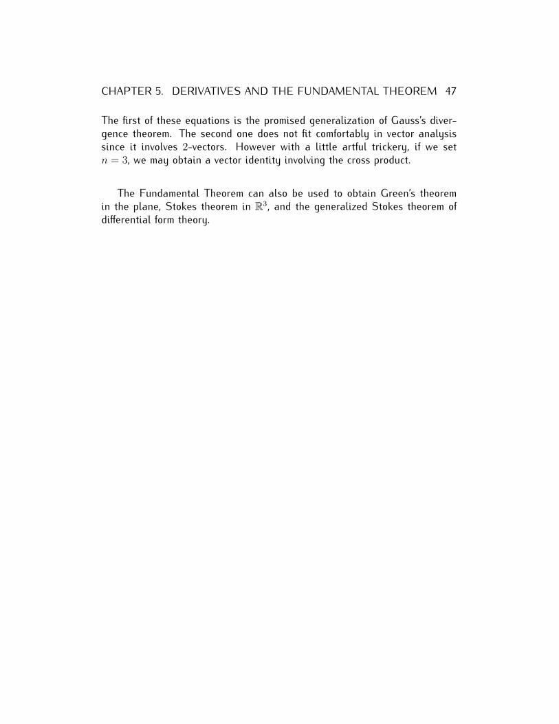
The first of these equations is the promised generalization of Gauss’s diver-gence theorem. The second one does not fit comfortably in vector analysissince it involves 2-vectors. However with a little artful trickery, if we setn = 3, we may obtain a vector identity involving the cross product.

The Fundamental Theorem can also be used to obtain Green’s theoremin the plane, Stokes theorem in R3, and the generalized Stokes theorem ofdifferential form theory.

Bibliography

[1] Alan Bromborsky, An Introduction to Geometric Algebra and Calcu-lus, http://montgomerycollege.edu/Departments/planet/planet/

Numerical_Relativity/bookGA.pdf, November 2013.

[2] Chris Doran and Anthony Lasenby, Geometric Algebra for Physicists,Cambridge University Press, 2003.

[3] David Hestenes and Garret Sobczyk, Clifford Algebra to Geometric Cal-culus, D. Reidel, 1984.

[4] Kenneth Hoffman, Analysis in Euclidean Spaces, Dover, 2007.

[5] Mehrdad Khosravi and Michael D. Taylor, The wedge product and ana-lytic geometry, The American Mathematical Monthly 115 (2008), no. 7,623–644.

[6] Alan Macdonald, A Survey of Geometric Algebra and Geometric Calculus,http://faculty.luther.edu/ macdonal., 2010.

[7] , An elementary construction of the geometric algebra, Ad-vances in Applied Clifford Algebras 12 (2002), no. 1, Slightly improved:http://faculty.luther.edu/ macdonal.

[8] , Linear and Geometric Algebra, Alan Macdonald, 2010.

[9] , Vector and Geometric Calculus, Alan Macdonald, 2012.

[10] Piotr Mikusiński and Michael D. Taylor, An Introduction to MultivariableAnalysis from Vector to Manifold, Birkhäuser, Boston, 2002.

[11] Garret Sobczyk, New Foundations in Mathematics, The Geometric Con-cept of Number, Birkhäuser, 2013.

48

BIBLIOGRAPHY 49

[12] M. D. Taylor, An Introduction to Geometric Algebra and Geometric Cal-culus, unpublished manuscript.

Index

0-vector, 21-vector, 1, 22-vector

magnitude, 3simple, 2

Tx0M, 21ΛkRn, 11Ck, 19I, 22k-vector, 1, 2

angle between two k-vectors, 16magnitude, 16simple, 2

angle, 16angle between parallelepipeds, 10angle between subspaces, 10

binomial coefficient, 13blade, 23

cell, 22chain rule, 36, 38change-of-variables formula, 24coordinate patch, 21–22, 25

nonsingular, 22coordinates, 25

differentiability, 19differentiable, 20differential, 20, 36directed line segment, 1

directional derivative, 19, 36division, 33–34dot product, 8, 15, 31

frame, 35

geometric algebra, 27, 28geometric derivative, 38–39geometric product, 9, 27, 29grade, 28

hyperplane, 18–19

induced orientation, 42left-hand, 42right-hand, 42

integraloriented, 27unoriented, 26

Jacobian determinant, 24

linenonparametric equation, 18

magnitude, 322-vector, 3k-vector, 16

multi-index, 14ordered, 14

multivector, 28magnitude, 32reversion, 31

50

INDEX 51

nonorientable surface, 24nonsingular, 22

opposite orientation, 4orientable surface, 24orientation, 5, 23, 24

arc, 23incomparable, 4non-comparable, 6opposite, 4, 6same, 4, 6surface, 24

oriented integral, 27, 40

parallelepiped, 4degenerate, 5vertices, 4volume, 5

parametrization, 21–22local, 21nonsingular, 22

reciprocal basis, 35, 38reciprocal frame, 35reciprocal vector, 35reversion, 9, 14, 30–31

multivector, 31

same orientation, 4scalar product, 31–32simple 0-vector, 6simple 2-vector, 2, 4simple k-vector, 2, 4, 6

multiplication by a scalar, 7wedge product, 10

space of k-vectors, 11dimension, 13

space of tangent vectors, 21standard basis vectors, iv

surface, 20Cr, 21

tangent p-vector, 23tangent vector, 21–22

space of tangent vectors at a point,21

translation of a set, 18

unit cube, 22unit interval, 22unoriented integral, 26

vector derivative, 39vector space axioms, 11

wedge product, 10, 12, 32–33

Documents

A Crash Course in Geometric Algebra and Geometric Calculus · geometric algebra and geometric calculus, somewhat in the spirit of Alan Macdonald’s A Survey of Geometric Algebra