Department of Economics and Finance

Working Paper No. 09-11

http://www.brunel.ac.uk/about/acad/sss/depts/economics

Econ

omic

s an

d Fi

nanc

e W

orki

ng P

aper

Ser

ies

Tomoe Moore

A critical appraisal of McKinnon’s complementary hypothesis: Does the real rate of return on money matter for investment in developing countries?

February 2009

1

A critical appraisal of McKinnon’s complementary hypothesis: Does the real rate of return on money matter for investment in

developing countries?

Tomoe Moore

Department of Economics and Finance, Brunel University

Uxbridge, Middlesex, UB8 3PH, United Kingdom

Tel: +44 189 526 7531

Fax: +44 189 526 9770

tomoe.moore@brunel.ac.uk

2

A critical appraisal of McKinnon’s complementary hypothesis: Does the real rate of return on money matter for investment in

developing countries?

Abstract

McKinnon’s (1973) complementary hypothesis predicts that money and investment are complementary due to a self-financed investment, and that a real deposit rate is the key determinant of capital formation for financially constrained developing economies. This paper critically appraises this contention by conducting a vigorous empirical approach by using panel data for 108 developing countries over the sample period of 1970-2006. The long-run and dynamic estimation results based on McKinnon’s theoretical model are supportive of the hypothesis. However, when the investment model is conditioned by such factors as financial development, different income levels across developing countries, external inflows, public finance and trade constraints, the credibility of the hypothesis has been undermined.

Keywords: Real deposit rates, Capital formation, Developing economies, Money, McKinnon’s complementary hypotheses

JEL Classification: E4, O1

3

1. Introduction

The assertion of self-financed capital formation for financially constrained developing

economies led McKinnon (1973) to develop a complementary hypothesis whereby a high real

return on money induces the accumulation of a real money balance, and this, in turn, finances

the costly, indivisible fixed capital. The hypothesis formulates a dual process, in which the

demand for real money balances depends directly, inter alia, on the average real return on

capital, and the investment ratio to GDP rises with the real deposit rate of interest. This

process provided a plausible empirical framework for researchers in analysing investment

decisions and a demand for money function for developing countries. Most literature

engages in a single equation framework, either a money or an investment equation. See, for

example, DeMelo and Tybout (1986), Edwards (1988), Morriset (1993), which focused on

the investment equation, and Harris (1979), Thornton and Poudyal (1990), who modelled a

demand for money function. The study of Fry (1978), Laumas (1990), Thornton (1990) and

Khan and Hasan (1998) has tested the complementarity hypothesis by estimating both

investment (or savings) and the demand for money functions. Pentecost and Moore (2006)

investigated the interdependence between the investment and money legs of the joint

hypothesis in a simultaneous system of equations for India. In all, the coverage of a sample

country is either single country or a group of several countries, and the empirical literature

tends to support the complementary hypothesis.

This paper critically appraises McKinnon’s complementary hypothesis by conducting

a vigorous empirical approach using panel data for 108 developing countries with the sample

period of 1970 to 2006. First, we test a panel cointegration for the key variables of money,

investment, real return on money, aggregate income and credit. The presence of

cointegration is a pre-requisite for the acceptance of the hypothesis. Then, the long run

relationship is modelled in a panel system of equations, followed by an error correction

4

dynamic model. We further extend the theoretical model by conditioning the investment

behaviour by incorporating the effect of financial development, different income levels across

developing countries, external inflows, trade constraints and public finance. These variables

are mostly predicted to raise the capital formation independently of the hypothesis.

We find a cointegration relationship among the key variables, providing a necessary

condition for the complementarity hypothesis. The long-run and dynamic estimates are

supportive, too, since we find a statistically significant effect of return on capital on the

demand for money model, and also a significant positive impact of real deposit rates on

investment. Evidence reveals that financial development and the status of a middle-income

level among developing economies are factors, which reduce self-financed capital formation

by mitigating financial constraints. The conditional variables are found to boost the economy

by accumulating the physical capital independently of the self-finance hypothesis. Although,

even after augmenting the investment model with the conditional variables, real deposit rates

are found to be statistically significant, the size of the coefficients is numerically too marginal

to provide vital evidence of self-financed capital formation. The empirical result highlights

the key role of financial intermediation through the conduit of credit for increased capital

formation.

The structure of the paper is as follows. In Section 2, McKinnon’s (1973)

complementarity hypothesis is specified. Section 3 describes the data employed for

estimation, and Section 4 spells out the panel unit root and cointegration tests. Long-run and

dynamic models are estimated in Section 5. In Section 6, the investment long-run model is

augmented with conditional variables. Section 7 concludes.

5

2. McKinnon’s complementarity hypothesis

McKinnon (1973) asserts self-finance and lump-sum expenditure or indivisibilities of

investment for financially-constrained developing countries, hence investors are obliged to

accumulate money balances prior to their investment project. Meanwhile, in many

developing countries, the decades of high budget deficits had resulted in high domestic

borrowings by the government. Government securities at low interest rates were one of the

major causes of financial repression, where interest rates were set by administrative decision,

which were likely to be below the market-determined levels (Fry 1980). McKinnon

emphasises that the removal or relaxation of the administered interest rates would boost

capital formation, since the high deposit rates attract the accumulation of money, and

stimulate investment.

The complementary hypothesis is examined using the dual models. First, the demand

for real money balances (M/P) depends positively upon real income, Y , the own real rate of

interest on bank deposits, d - πe (d = deposit rates and πe = expected rate of inflation), and the

real average return on capital, c. The positive association between the average real return on

physical capital and the demand for money balances represents the complementarity between

capital and money as given by (time scripts are omitted for simplicity).

)d,c,Y(P/M eπ−Ψ= 000 >Ψ>Ψ>Ψ− edcY ,,π

(1)

The equation (1) suggests that the demand for money is given not only by the transactions

and speculative motive of holding cash but also by the need to finance real capital formation

in countries, where institutional credit or alternative finance are constrained. There is also the

need to hedge against inflation in such a way as to preserve the real value of money balances.

The complementarity works in both directions: money supply has a first order impact

in determining investment, hence the complementarity can be accomplished by specifying an

investment function given by:

6

)d,c(FY/I eπ−= 00 >>− edr F,Fπ

(2)

The investment to income ratio, I/Y, must be positively related to the real rate of return on

money balances. This is because if a rise in the real return on bank deposits, d - πe raises the

demand for money, and real money balances are complementary to investment, it must also

lead to a rise in the investment ratio. The complementarity hypothesis specifically requires

that 00 >>Ψ− edc Fandπ

1.

McKinnon’s model is, however, restrictive in that it is assumed that there is no role of

intermediation by financial institutions from saving (money includes current and time savings) to

the creation of credit. This is very unlikely even in under-developed financial markets.

Since the indirect effect of real deposit rates on investment is due not only to self-finance, but

also to the credit creation from money, where the real supply of credit increases pari passu

money demand (Fry 1980). Moreover, the level of credit may contain two types of

information about the process of financial intermediation. First, changes in credit may reflect an

ability of financial intermediaries to make loans perhaps due to changes in monetary policy. In

this case, firms, which are unable to obtain funds in the capital market may become credit-

constrained leading to lower levels of investment. Second, changes in credit may reflect shocks

to the intermediation system itself. In particular, financial liberalisation undertaken in many

developing countries initiates various forms of deregulations in financial markets, the creation

of financial innovations, or changes in the solvency of borrowers or lenders, which has

implications for economic activity that may be transmitted through changes in the quantity of

credit (Mallick and Moore 2008). In this respect, the availability of credit to business will

affect the investment ratio independently of the self-finance motive of holding money, hence

the variable of ‘credit’ is specified in the investment equation (2). By specifying credit along                                                             1 Shaw (1973) argues that complementarity has no place here because investors are not constrained to self-finance. Shaw had the debt-intermediation view by specifying a vector of real opportunity costs (real yields on all types of wealth) of holding money in equation (1).

7

with the real rates of deposit in the investment equation, the two channels of funding sources

could be identified: one is self-finance portrayed by the effect of real deposit rates, and the

other channel is through credit intermediated by financial institutions.

From an empirical perspective, since it is impossible to compute a sensible measure of

the real return on physical capital, McKinnon (1973) suggests that it could be replaced by the

investment to income ratio, I/Y, which is likely to vary directly with the average real return on

capital (see also Pentecost and Moore 2006). The models now become:

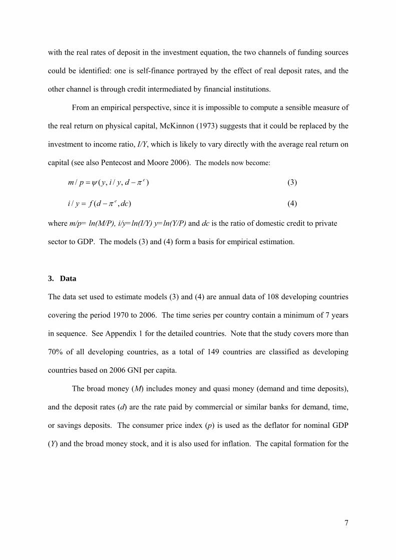
),/,(/ edyiypm πψ −= (3)

),(/ dcdfyi eπ−= (4)

where m/p= ln(M/P), i/y=ln(I/Y) y=ln(Y/P) and dc is the ratio of domestic credit to private

sector to GDP. The models (3) and (4) form a basis for empirical estimation.

3. Data

The data set used to estimate models (3) and (4) are annual data of 108 developing countries

covering the period 1970 to 2006. The time series per country contain a minimum of 7 years

in sequence. See Appendix 1 for the detailed countries. Note that the study covers more than

70% of all developing countries, as a total of 149 countries are classified as developing

countries based on 2006 GNI per capita.

The broad money (M) includes money and quasi money (demand and time deposits),

and the deposit rates (d) are the rate paid by commercial or similar banks for demand, time,

or savings deposits. The consumer price index (p) is used as the deflator for nominal GDP

(Y) and the broad money stock, and it is also used for inflation. The capital formation for the

8

private sector (I) is derived from the gross fixed capital formation2. All these data are taken

from World Development Indicators.

Expected inflation in d-πe is not directly observable. For a volatile rate of inflation in

developing economies, where the future prediction of the variable is extremely difficult, an

autoregressive type of expectation seems to be reasonable3. We take a naïve expectation, i.e.

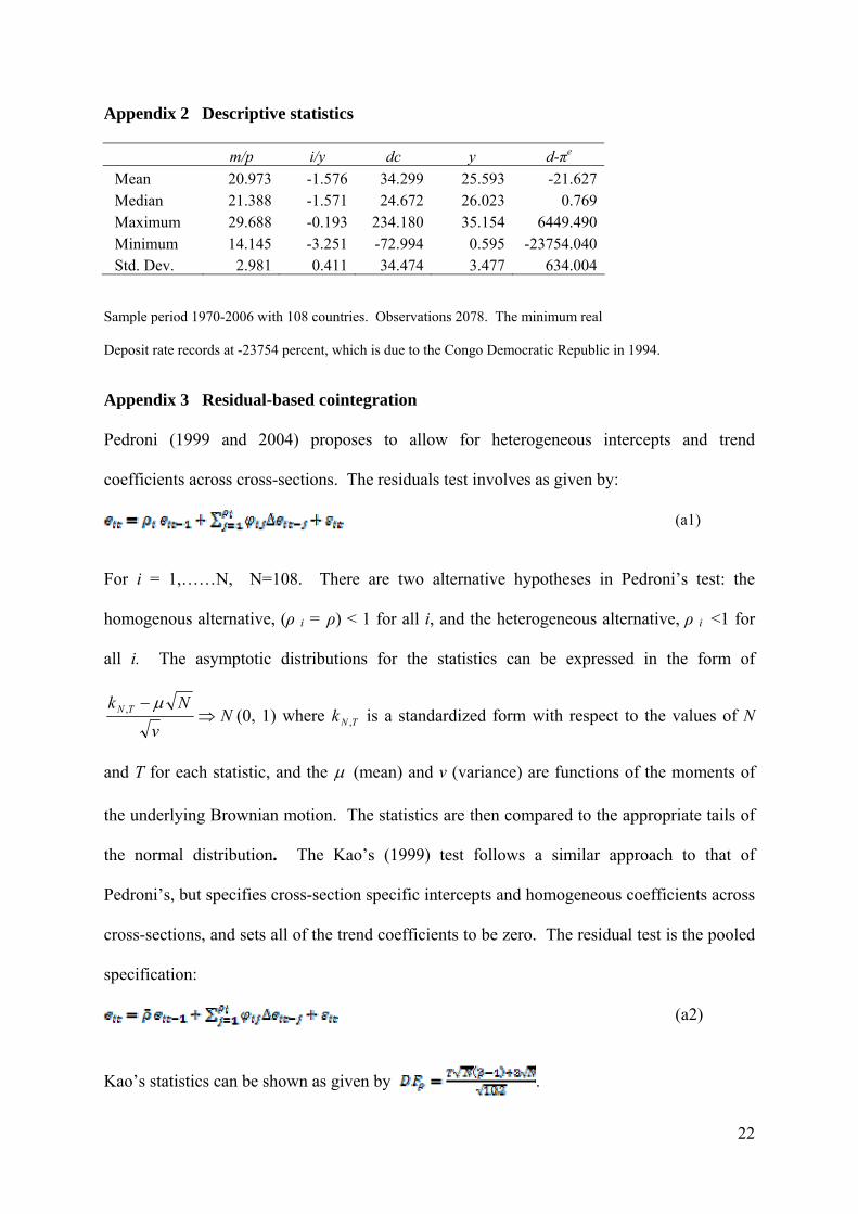
tet ππ =+1 . The descriptive statistics are found in Appendix 2.

4. Panel unit root and cointegration tests

The complementarity hypothesis predicts the linkage between money and investment, and

that the dependent and independent variables in equations (3) and (4) are likely to form a

stable long-run relationship. Hence, we conduct a unit root and cointegration tests in this

section.

Unit root tests

It is argued that Fisher’s ADF and PP tests proposed by Maddala and Wu (1999) would fit for

unbalanced panel data. Maddala and Wu (1999) assume individual unit root process, and

combine the p-values from individual unit root tests. The test statistics are the asymptotic

We also conduct two other types of panel unit root tests, developed by Levin et al. (2002) and

Im et al. (2003) for the robustness check. Levin et al. (2002) assume that there is a common

unit root process so that coefficients on the lagged dependent variables are homogeneous

across cross-sections, though incorporates a degree of heterogeneity by allowing for fixed

effects and unit specific time trends. In contrast, Im et al. (2003) allow for heterogeneity of

                                                            2 The gross fixed capital formation includes plant, machinery, office, equipment purchases, private residential dwellings, commercial and industrial buildings and also the construction of roads, railways, schools and hospitals. There is no data available exclusively for the private investment for many of these developing countries. Hence, we take a ratio of private sector consumption expenditure to total consumption expenditure (private and government sectors), as a weight on the gross fixed capital formation to derive the private sectorinvestment. 3 An earlier study by Khan (1988) found that the results were not sensitive to alternative expectations including perfect foresight, static expectations and adaptive expectations.

9

the coefficients on the lagged dependent variable with the slope coefficients to vary across

cross-sections. The null is that all series are nonstationary, whilst the alternative is that at

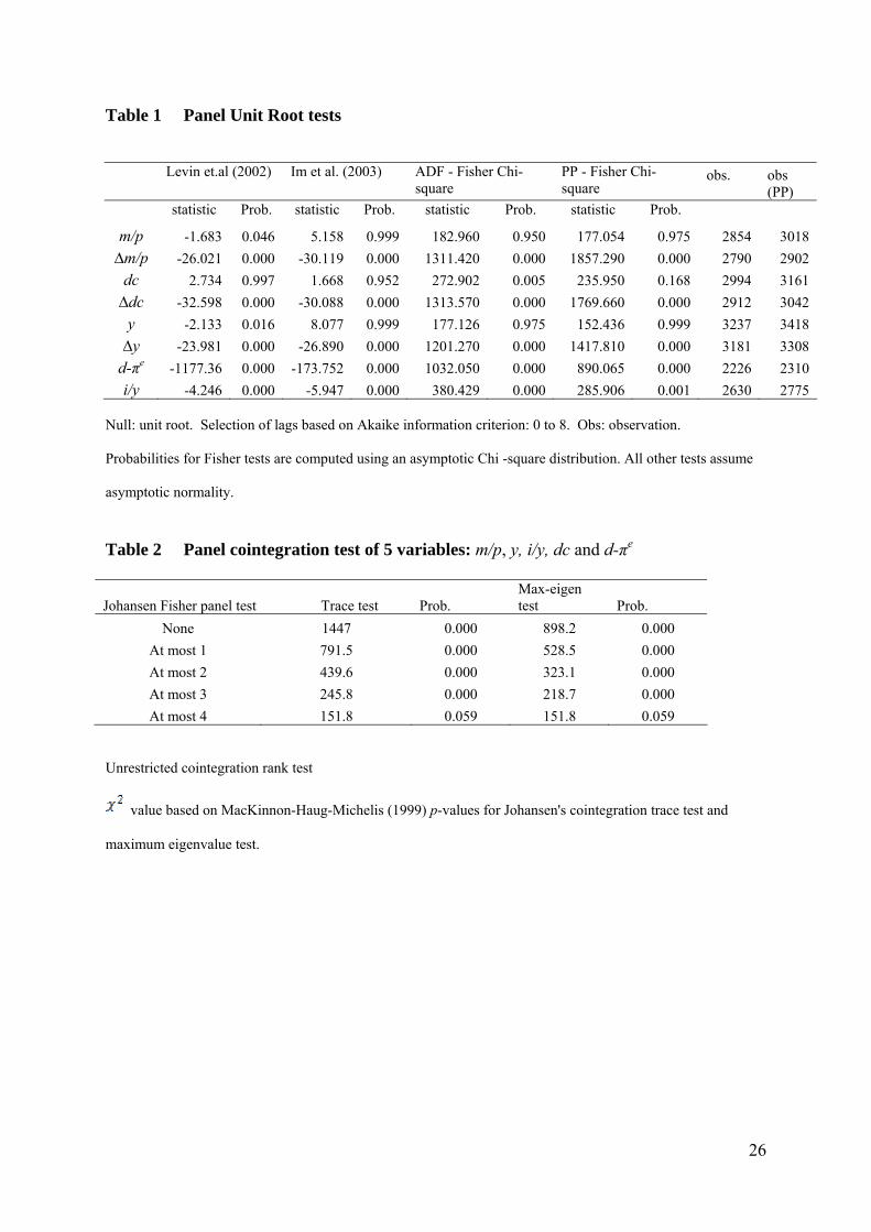
least one cross-section is stationary. See Table 1 for the results.

[Table 1 around here]

The variables of m/p, dc and y in levels are found to be insignificant at the 5% level implying

that they are non-stationary. The first difference of these variables rejects the null of unit

root4. It follows that these variables are characterised as integrated of order one, I(1). The

null is rejected for i/y and d-πe in levels, hence they are stationary, I(0).

The unit root test result means that there are I(0) and I(1) mixed in analysing

cointegrating relationship. The presence of some I(0) variables in the regressions does not vitiate

the test for cointegration. I(0) variables might play a key role in establishing a long-run

relationship between I(1) variables, in particular, if theory a priori indicates that such I(0)

variables should be included 5.

Panel cointegratin test

The cointegration test is conducted for the five variables of m/p, y, i/y, dc and d-πe. Since we

are analyzing the cointegrating properties of a n >2 dimensional vector of I(1) variables, in

which up to n-1 linearly independent cointegration vectors are possible. Hence, the Johansen

cointegration test is appropriate. Fisher (1932) derives a combined test that uses the results of

the individual independent tests. Maddala and Wu (1999) extend the Fisher’s test by

developing a Johansen panel cointegration test, which combines tests from individual cross-

sections for the full panel. If ωi is the p-value from an individual cointegration test for cross-

section i, then under the null hypothesis for the panel, we have .

[Table 2 around here]                                                             4 Note that Levin et al. (2002) suggests that y and m/p in levels are significant at the 5% level, implying the variables is I(0). Yet, the Im et al. (2003) and Fisher tests are not rejected, and that we treat them as I(1). 5I(0) variables may contribute to a sensible long-run relationship among I(1) variables (Harris, 1995).

10

The test result is shown in Table 2. The trace and maximum eigenvalue tests suggest that

there are 4 cointegrating vectors at the conventional significance level. Note that the

inclusion of I(0) variables (i.e. i/y and d-πe ) increases the number of cointegration vectors,

since each I(0) variable is stationary by itself, and it forms a linearly independent

combination of the variables, which is stationary6. The presence of cointegration suggests

that there is a long-run stable relationship existing amongst these variables. If the real deposit

rates affect money, which in turn affect credit, hence investment, then the cointegration

relationship is a conventional standard result. If there is a direct effect of money on the

formation of physical capital, the presence of cointegration is a prerequisite for the

complementarity hypothesis7.

5. Long- run and dynamic error-correction model

Long-run model

In panel estimations, the existence of unobservable determinants can be decomposed into a

country-specific term and a common term to developing countries. The unobservable

country-specific determinants can be taken into account in the estimation procedure, and the

models (3) and (4) respectively become:

m/p it = ßi,0 + ß1yi,t+ ß2i/yit + ß3 (d-πe)it + εit (5)

i/y it = αi,0 + α1 (d-πe)it + α2 dcit + εit (6)

                                                            6 Dickey et al. (1994) argue that cointegration vectors may represent constraints on the movement of the variables in the system in the long-run, and consequently, the more cointegrating vectors there are, the more stable the system is. 7 Some empirical literature finds cointegration (see Table 4 in this paper) and claims it as compelling evidence of the complementarity hypotheses. This overrates the finding.

11

ßi,0 and αi,0 are a time-invariant individual country effect term and εit is an error term8. It is

possible that country specific terms improved the estimates by absorbing country specific

errors and reducing heteroskedasticity.

The cross-country regressions are subject to endogeneity problems. For example, the

correlation between real deposit rates and money could arise from an endogenous

determination of real rates, that is, real rates themselves may be influenced by innovations in

the stochastic process governing the variable of money. Also any omitted factors may

increase both real rates and money simultaneously. In these circumstances there would exist

a correlation between real deposit rates and the country-specific error terms in equation (5),

which would bias the estimated coefficients. The endogeneity problem can be mitigated by

applying instrument variable (IV) techniques. A good instrument would be a variable which

is highly correlated with regressors, but not with the error terms. We use the lagged values

of regressors and dependent variables in each equation. Besides, money is included as an

instrument variable in the investment equation, and credit is in the money equation. This is

not only due to the complementarity consideration, but also to the following reasons: Under

disequilibrium financial conditions, where real deposit rates could be administered, being

below equilibrium level, real credit supply is determined by real money demand and there is

likely to be little direct feedback mechanism from investment demand to real credit. As there

is limited supply (of savings), the volume of investment is determined solely by conditions of

supply. In this respect, the use of money, as an instrument variable deals with any

simultaneous equation bias in the investment estimate.   However, where interest rate ceilings

are relaxed or removed, a larger demand for investible funds will elicit an increase in quantity

                                                            8 The period effects are found to be insignificant by the likelihood ratio test, therefore we do not specify the period dummy. It is possible that the regressors may capture some of the shifts in the economy over the sample period. In the next section, when the model is augmented, such period effects are likely to be subsumed in the controlled variables, hence there is not much concern.

12

supplied through higher returns to savers. This consideration dictates the inclusion of credit

as an instrument variable in the money equation.

By using the IV techniques, we estimate the models in two ways: one is in a single

equation framework, where money and investment are modelled separately, and the other is

in a system of simultaneous equations, where both equations are simultaneously estimated.

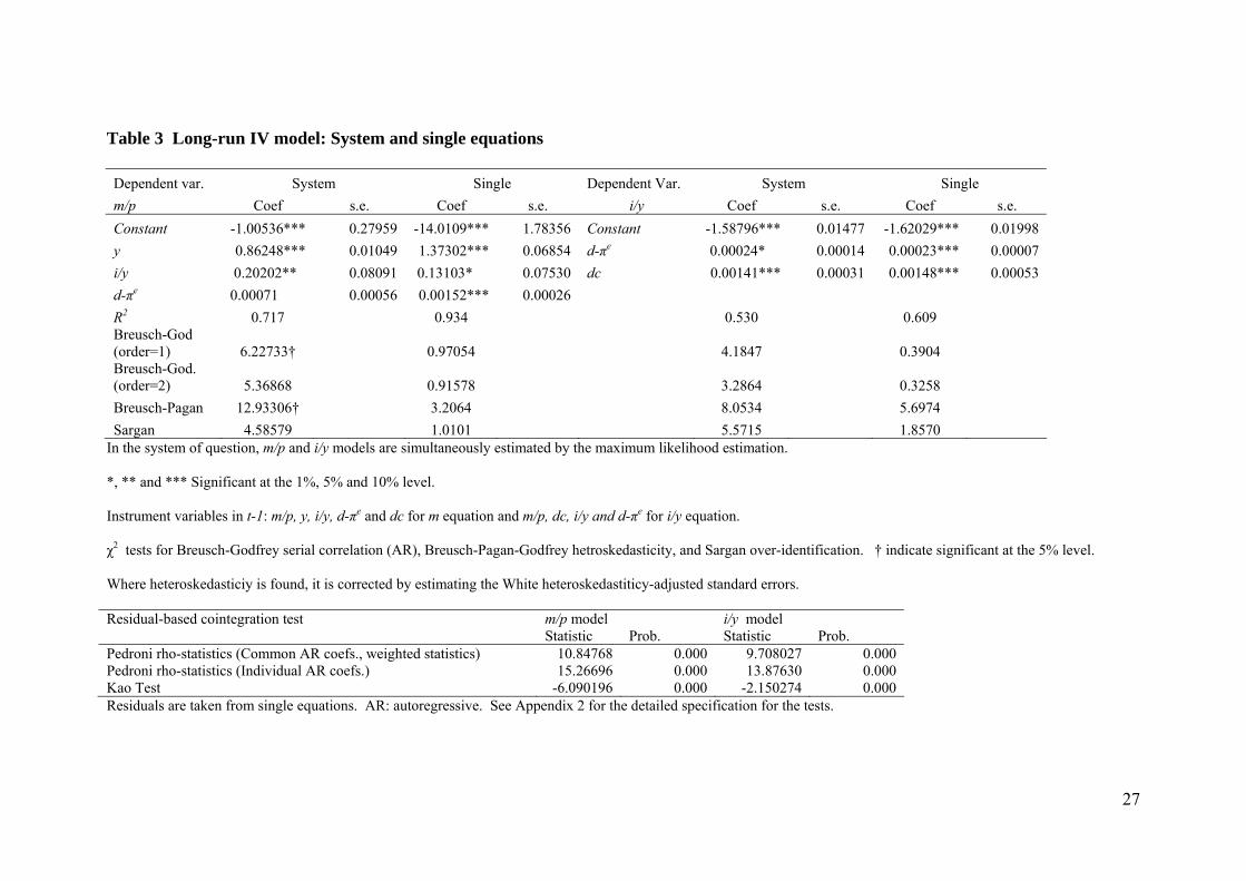
The estimates of the long-run models are shown in Table 3. An estimator that uses lags as

instruments under the assumption of white noise errors would lose its consistency if, in fact,

the errors were serially correlated. It is, therefore, essential to satisfy oneself that this is not

the case by reporting test statistics of the validity of the instrument variables. We present the

first and second order residual serial correlation coefficients and the Sargan test of over-

identifying restrictions together with the Breusch-Pagan-Godfray heteroskedasticity test. We

also conduct the residual-based panel coingegration test of Pedroni (1999, 2004) and Kao

(1999) for each single equation (see Appendix 3 for the specification). It is shown in Table 3

that these residual tests are, in general, satisfactory, and the evidence of stationarity of the

residuals seems to steer clear of ‘spurious’ regression.

[Table 3 around here]

The signs of all the coefficients agree with a priori expectations with a statistical

significance, except for the real deposit rate in the system of money equation, which fails to

reach the 5% significance level. In the money model, the magnitude of the coefficients tends

to be larger in the single equation, as compared with that in the system equation. The

investment model shows a remarkably similar size of coefficients between the system and

single equations.

The positive relationship of the demand for money with the level of aggregate income

accords with the transactions demand for money hypothesis. The sizes of the coefficient at

0.86 and 1.37 in the system and single equations respectively are quite plausible, being

13

similar to those found in the empirical literature on the demand for money for developing

economies9. The positive impact of the investment income ratio on money supports the

assumption of self-finance and indivisibility. Thus where self-finance is important, a rise in

i/y increases rather than decreases m/p. The estimated coefficient suggests that one

percentage point increase in the investment ratio would increase the real money stock by

about 0.20 to 0.13 percentage points. In the investment model, it is evident that the

availability of credit raises the investment ratio, and the positive relationship with d-πe

highlights the importance of high real rates of interest for capital accumulation. A crucial

finding is the significant positive sign on i/y in the money function and d-πe in the investment

function, which provide robust empirical support for the complementarity hypothesis

according to McKinnon’s (1973) theory.

Financial repression is deemed to be the holding of institutional interest rates,

particularly of deposit rates of interest, below their market equilibrium levels. Our empirical

evidence reveals that under disequilibrium interest rate conditions, higher deposit rates raise

capital formation via the increase in real money balances, where money is defined broadly to

include savings. The supply of credit is also due to the increased deposit rates, yet if there is

a credit control prevalent10 and if we also consider such factors as external inflows and

international trade in developing economies, there is a limitation in treating it as solely a

direct consequence of the increased rates11. In this respect, the positive influence of deposit

rates on investment is instinctive in terms of the self-financed fixed capital, and proves to be

a credible sign of the complementarity hypothesis.

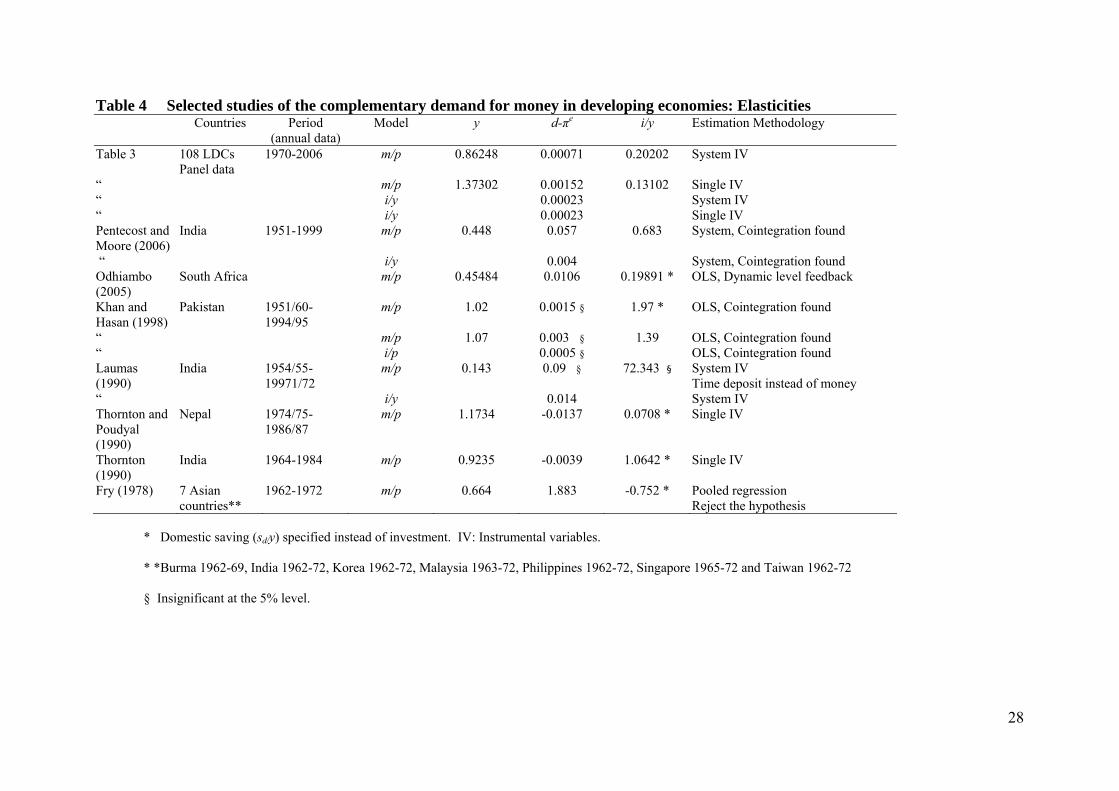
[Table 4 around here]

                                                            9 See the selected studies in Table 11 in Moore et al. (2005) for the income elasticities of the demand for money. 10 The monetary authorities may generate new credit independently of domestic saving often in response to government policy. 11 The supply of real credit is also determined by the balance of payments situation (Leff and Sato 1980) .

14

For a comparative study, we present selected studies of the complementarity

hypothesis in Table 4, where the elasticities of level feedback are available in a similar model

specification to that of this paper. The income elasticity (y) ranges from 0.45 to 1.17 in the

literature and our estimates are quite comparable. The real deposit rate elasticity is relatively

small with at 0.00152 in m/p model, which is closer to that of Khan and Hasan (1998). The

interest rate elesticity is much smaller in the i/y model at around 0.00023. Such a low

magnitude is again found for Pakistan at 0.0009 by Khan and Hasan (1998). The study of

Fry (1978) rejects the complementarity hypothesis since domestic saving is found to be

negative for seven of the less developed countries (LDCs) in Asia in a pooled demand for

money regression12.

Dynamic error correction model

In order to ascertain credibility of the long-run estimates, we investigate the dynamic

behaviour of the demand for money and investment. Dynamic modelling in a system of

equations is, however, not practically plausible with the small sample size in terms of time

series relative to the number of explanatory variables: for example, the total of sixteen

variables with one lag for each explanatory variable are to be simultaneously solved. Also

given the fact that there is not a sizeable difference in estimates between the system and

single equations in Table 3 in the long-run model, we estimated the dynamic model in a

single equation with the IV technique.

[Table 5 around here]

Tables 5 presents the dynamic, error correction model, where the lagged error correction

terms (et-1) which are the residuals taken from the single equation of the long-run model, are

specified along with the other explanatory variables by taking one lag for each. The

                                                            12 Fry (1978) specified domestic saving in the place of investment on the ground that a self-financed hypothesis excluded foreign saving.

15

respective error correction terms are found to be highly significant in each equation with the

correct negative sign, indicating the appropriateness of the identified long-run relationships.

The explanatory variables are statistically and theoretically well-determined in the

money equation: the level feedback from income, investment and real rates of interest is

correctly signed. The negative impact from the lagged deposit rates on the real money

balance may be interpreted as the adjustment effect. In the case of the investment function,

again the level feedback is statistically significant with a correct sign. The size of the

coefficient on the real interest rates is halved to 0.00011 when compared with that in the

long-run. The overall results appear to strengthen those of the long-run model.

6. Augmented investment model

In the seminal work of McKinnon’s (1973) complementarity hypothesis, government fiscal

action has little role in affecting directly aggregate capital accumulation, since the public

policy is limited to the control of the real return on holding money, i.e. (d-πe). Further

restrictions apply to the simplified assumptions about investment in small self-financing

domestic enterprises. The models described are also derived from the assumptions of a

closed economy, even though empirical materials are usually drawn from small open

economies, and so their rates of capital formation are unlikely to be determined solely by tiny

self-financing units. Virtually, many developing countries are highly dependent on foreign

trade and are open to corporate investment from abroad. Hence, a rise in investment may not

be always due to a rise in the saving ratio when foreign trade or foreign capital flows are

brought into the picture. McKinnon (1973) also fails to take account of the effect of financial

development and the different income levels across countries, as these are treated as constant.

We relax these assumptions or restrictions by augmenting the long-run investment models

16

with several factors, which are likely to contribute to the share of financing in domestic

capital formation.

Firstly, we consider financial development, which develops financial innovations and

deregulates some restrictions in the capital market widening the scope for alternative

investment opportunities, and also removes barriers to foreign banks. This is likely to impact

on the transmission mechanism between deposit rates and investment. As a proxy variable,

we explicitly include the development of stock market and a broad money13. The latter may

represent financial sector deepening 14 . Secondly, the model is designed to reflect the

different levels of income across developing countries. Depending on the level of

institutional capability, the bureaucratic efficiency, technological capability and the quality of

labour, deposit rates may affect investment differently. Assuming that these factors are,

though in a crude manner, subsumed in the level of income, the estimation is conducted by

taking dummy variables for the two income groups of low and upper-middle countries to see

if there is any difference in the linkage15.

Thirdly, external flows such as FDI (foreign direct investment) and ODA (official

development assistance) are likely to affect capital formation independently of the level of

real deposit rates. Foreign capital takes various forms. FDI implies long-term investment

consisting of not only capital per se, but also management skill, know-how and technology,

and FDI transmits technological diffusion from the developed countries to the developing

countries raising capital formation (Balasubramanyam et al. 1999 and Borensztein et al.

1998). Short-term foreign capital flows include portfolio investment and foreign bank

lending. FDI is specified separately from the short-term foreign loans, since the latter depend

                                                            13 The variable of credit is combined with these variables, so that they capture the financial development in a wider range. 14 One may prefer to hold monetary assets only when it is felt convenient to keep ones’ wealth in monetary instruments with an underlying nature of liquidity, risk, return and efficiency in payment. Such types of instruments are offered by a better developed financial sector. 15 In the preliminary result, the lower-middle income countries performs poorly, hence we concentrate on low and upper-middle income groups.

17

on the development of the domestic financial market, thus it is assumed to be captured

through the variable of credit 16 . ODA includes aid or concessional funds from such

institutions as the IMF and the World Bank, and distinguishes itself from FDI, therefore ODA

makes a separate entry to the model. Fourthly, we address the extent to which the public

spending is transmitted into capital and production17. We condition the investment decision

in the private sector involving the improvement of infrastructure or purchase of public

capital18.

Lastly, some attention is paid by the literature to the foreign trade constraint to

economic growth. Openness and trade policy are important for productivity spill-over and

the cost of capital goods. More open economies have experienced faster productivity growth

(Edwards 1998 and Diao et al. 2005), and developing countries can boost their productivity

by importing a larger variety of intermediate products and capital equipment which embody

foreign knowledge (Coe et al. 1997). A variable of the foreign trade is added as a

conditional instrument.

The augmented investment model is now given by:

),,(/ vdcdfyi eπ−= (7)

where v is the vector of additional explanatory variables: fdit (financial development), fdiit

(FDI), odait (ODA) , git (government expenditure) , tradeit (foreign trade) and income dummy

for a low and upper-middle income groups. fd and income dummy are specified as an

interaction with the real deposit rates. Financial development is the sum of the three ratios of

stock market capitalization, M2 and domestic credit to GDP. FDI, ODA, foreign trade, and

government expenditure are also all percentage of GDP. The country-income groups can be

                                                            16 See, for example, Bosworth and Collins (1999) for justification. 17 For example, Chatterjee and Turnovsky (2007) argue that the effectiveness of foreign capital on investment depends on the condition of the public finance. 18 In some developing countries, much of the government expenditure could be allocated to government consumption or defence, rather than productive projects, and if this is stronger, public expenditure would have a negative impact on private investment.

18

found in Appendix 2. The data are all retrieved from the World Development Indicator. The

estimation is conducted by the IV model with a country-specific dummy.

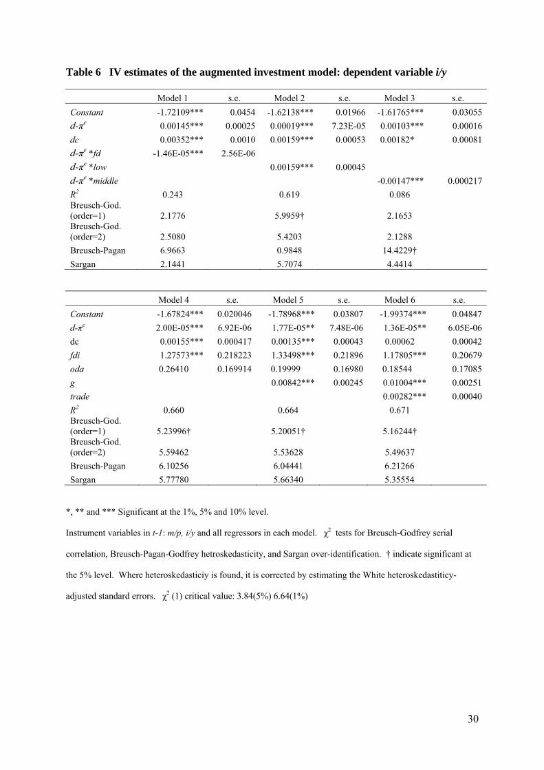
[Table 6 around here]

Empirical results are reported in Table 619. The coefficient on the interaction of deposit

rates with financial development in Model 1 is negative. As the scope for obtaining funds

from capital markets increases, reliance on self-finance may be curtailed. In Model 2 and 3,

the interaction between the real deposit rate and the upper-middle income group is shown to

be negative, whereas that for the low-income countries is positive. This implies that as the

status of a developing country moves from the low to the middle income group, there is less

self-finance in investment. These results are not surprising and explain why some empirical

literature rejects the hypothesis. For example, Fry (1978) finds that money is not the only

financial repository of domestic saving for the seven Asian semi-industrial LDCs. This is

because these countries have achieved stages of financial development well beyond the phase

in which the complementarity assumptions predominate20. Similarly, in the empirical work

for 25 Asian and Latin American LDCs, Gupta (1984) did not find a strong support for the

complemetarity hypothesis. It is noted that some of the major Latin American countries in

Gupta’s study are classified as being in the upper-middle income bracket.

The impact of FDI and ODA in Model 4 also accords with a priori expectations,

indicating that as the external flow increases the amount of investment is raised, being

independent of the complementarity hypothesis21. Note that the effect of ODA on capital

formation is weak, as the coefficient is not significant. Generally, in order for ODA to affect

output most effectively, countries need to be equipped with reasonably developed institutions

                                                            19 The models, in general, tend to suffer a first-order serial correlation at the 5% level, but it is not rejected at the 1% level. The second-order serial correlation is not rejected at the 5% level in all cases. 20 In Fry’s (1978) study, three out of the seven countries are not even categorised as developing countries now. 21 Empirically, the impact of FDI on economic growth has remained controversial. Our results are in line with e.g. Blomstrom et al. (1996), Balasubramanyan et al. (1999) and Borensztein et al. (1998), who observe a positive impact.

19

and legal systems. Moreover, aid could be often misallocated into financing personal

consumption expenditure by the government or reserve accumulation (in particular when the

exchange rates are fixed), rather than increasing productive capital formation. These factors

may, in part, explain the insignificant effect of ODA. Public finance (Model 5) and trade

openness (Model 6) had a positive significant impact.

The robust finding is that d-πe is statistically significant, even when the investment

model is conditioned. It is, however, worth noting that there is a sharp fall in the magnitude

of the coefficient, when such factors as external flows, trade and public finance are specified

in the model. Meanwhile, the size of the coefficient on the credit remains to be robust, e.g.

the coefficients of 0.0015 and 0.0013 in Model 4 and 5 respectively in Table 6 are similar to

0.0014 in Table 3. The real rate of return on money matters in the creation of investment

opportunities due to a self-financed capital formation, however, given the numerically small

coefficient, the complementarity hypothesis is of very limited value.

7. Conclusion

This paper has extensively tested McKinnon’s complementarity hypothesis for 108

developing countries using panel cointegration and IV econometric techniques. The

empirical results reported, show that the real rate of interest has a positive effect on money

and investment, hence McKinnon’s stress on the importance of financial conditions in the

development process is justified. Our result substantiates the earlier findings for individual

countries for self-financed capital formation. However, at the same time, we find that the

influence of the real deposit rate on capital formation is numerically marginal, and its’ effect

fades when the investment model is augmented with conditional variables. It is also found

that the complemetarity is not supported in the middle-income group of countries, or when a

country reaches a certain stage of financial market development. In this respect, one may

20

have to look much farther down the development ladder, well below the middle-income level

of developing economies to the world’s least developed countries for recognising the

complementary theory.

The evidence highlights the strength of the credit link with the role of financial

intermediation. Under the disequilibrium interest rate system characterising most developing

countries, a decline in the real deposit rate of interest reduces real money demand, which

affects real credit supply, and this, in turn, squeezes new fixed investment. In either self-

financed or bank-loan financed capital formation, the real rate of return on money greatly

matters in raising the formation of capital. The central banks for developing economies

should continue to ensure a policy aimed at changing negative real interest rates to positive

levels, or improve the positive rates in order to secure greater levels of investment.

21

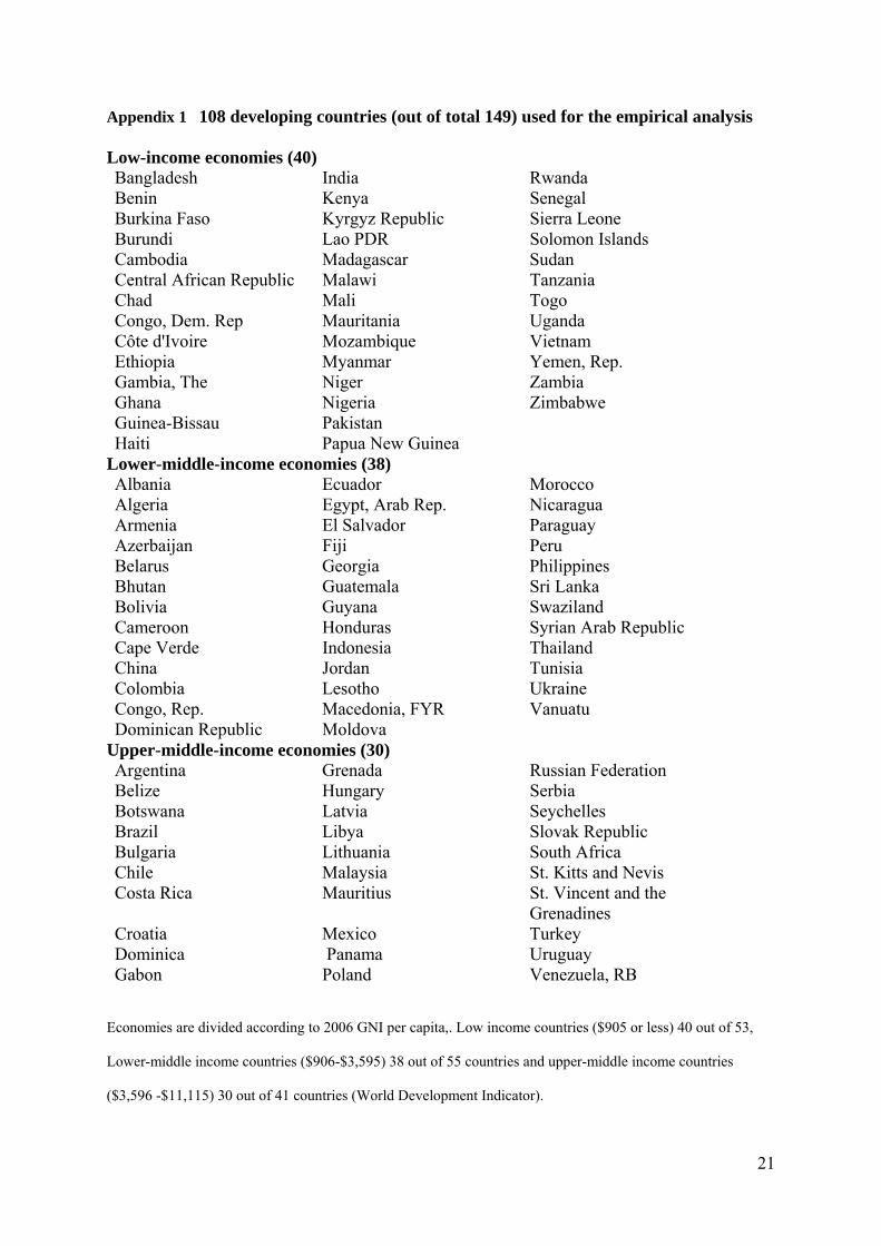
Appendix 1 108 developing countries (out of total 149) used for the empirical analysis

Low-income economies (40) Bangladesh India Rwanda Benin Kenya Senegal Burkina Faso Kyrgyz Republic Sierra Leone Burundi Lao PDR Solomon Islands Cambodia Madagascar Sudan Central African Republic Malawi Tanzania Chad Mali Togo Congo, Dem. Rep Mauritania Uganda Côte d'Ivoire Mozambique Vietnam Ethiopia Myanmar Yemen, Rep. Gambia, The Niger Zambia Ghana Nigeria Zimbabwe Guinea-Bissau Pakistan Haiti Papua New Guinea

Lower-middle-income economies (38) Albania Ecuador Morocco Algeria Egypt, Arab Rep. Nicaragua Armenia El Salvador Paraguay Azerbaijan Fiji Peru Belarus Georgia Philippines Bhutan Guatemala Sri Lanka Bolivia Guyana Swaziland Cameroon Honduras Syrian Arab Republic Cape Verde Indonesia Thailand China Jordan Tunisia Colombia Lesotho Ukraine Congo, Rep. Macedonia, FYR Vanuatu Dominican Republic Moldova

Upper-middle-income economies (30) Argentina Grenada Russian Federation Belize Hungary Serbia Botswana Latvia Seychelles Brazil Libya Slovak Republic Bulgaria Lithuania South Africa Chile Malaysia St. Kitts and Nevis Costa Rica Mauritius St. Vincent and the

Grenadines Croatia Mexico Turkey Dominica Panama Uruguay Gabon Poland Venezuela, RB

Economies are divided according to 2006 GNI per capita,. Low income countries ($905 or less) 40 out of 53,

Lower-middle income countries ($906-$3,595) 38 out of 55 countries and upper-middle income countries

($3,596 -$11,115) 30 out of 41 countries (World Development Indicator).

22

Appendix 2 Descriptive statistics

m/p i/y dc y d-πe

Mean 20.973 -1.576 34.299 25.593 -21.627 Median 21.388 -1.571 24.672 26.023 0.769 Maximum 29.688 -0.193 234.180 35.154 6449.490 Minimum 14.145 -3.251 -72.994 0.595 -23754.040 Std. Dev. 2.981 0.411 34.474 3.477 634.004

Sample period 1970-2006 with 108 countries. Observations 2078. The minimum real

Deposit rate records at -23754 percent, which is due to the Congo Democratic Republic in 1994.

Appendix 3 Residual-based cointegration

Pedroni (1999 and 2004) proposes to allow for heterogeneous intercepts and trend

coefficients across cross-sections. The residuals test involves as given by:

(a1)

For i = 1,……N, N=108. There are two alternative hypotheses in Pedroni’s test: the

homogenous alternative, (ρ i = ρ) < 1 for all i, and the heterogeneous alternative, ρ i <1 for

all i. The asymptotic distributions for the statistics can be expressed in the form of

Nv

Nk TN ⇒− μ, (0, 1) where TNk , is a standardized form with respect to the values of N

and T for each statistic, and the μ (mean) and v (variance) are functions of the moments of

the underlying Brownian motion. The statistics are then compared to the appropriate tails of

the normal distribution. The Kao’s (1999) test follows a similar approach to that of

Pedroni’s, but specifies cross-section specific intercepts and homogeneous coefficients across

cross-sections, and sets all of the trend coefficients to be zero. The residual test is the pooled

specification:

(a2)

Kao’s statistics can be shown as given by .

23

References

Balasubramanyam, V.N., M. Salisu, and D. Sapsford (1999). Foreign Direct Investment as an Engine of Growth, Journal of International Trade and Economic Development 8, 27-40.

Blomstrom, M., R. Lipsey and M. Zejan (1996). Is fixed investment the key to economic

growth? Quarterly Journal of Economics, 111(2), 269-276. Borenszstein, E. J. G and J.W. Lee, (1998). How Does Foreign Direct Investment affect

Economic Growth?, Journal of International Economics 45, 115-35. Bosworth, B.P. and S.M. Collins (1999). Capital flows to developing economies:

implications for saving and investment, Brookings Papers on Economic Activity, 1, 143-180.

Chatterjee, S. and S.J. Turnovsky, (2007) Foreign aid and economic growth: The role of flexible labor supply, Journal of Development economics, 84, 507-533.

Coe D., E. Helpman, and A. Hoffmeister (1997). North-South R & D spillovers, Economic

Journal 107, 134-149. De Melo, J. and J. Tybout. (1986). “The Effects of Financial Liberalisation on Savings and

Investment in Uruguay,” Economic Development and Cultural Change 34 (April): 561-587.

Diao X., J. Rattsø and H.E. Stokke (2005). International spillovers, productivity growth and

openness in Thailand: an intertemporal general equilibrium analysis, Journal of Development Economics, 76, 429-450.

Dickey, D.A., D.W. Jansen and D.L. Thornton (1994). A Primer on Cointegration with an

Application to Money and Income, in ed. Rao, B.B., Cointegration for the Applied Economist, St. Martin’s Press, Inc.

Edwards, S. (1988). Financial Deregulation and Segmented Capital Markets: The Case of

Korea, World Development 16 (1):185-194. Edwards, S. (1998). Openness, productivity and growth: what do we really know? Economic

Journal, 108, 383-398. Fry, M.J. (1978), Money and capital or financial deepening in economic development,

Journal of Money, Credit and Banking, 10 (November), 464-475. Fry, M.J. (1980). Saving, investment, growth and the cost of financial repression, World

Development, 8, 317-327. Gupta, K.L. (1984). Finance and economic growth in developing countries. London: Croom

Helm Ltd. Harris, J.W. (1979). An Empirical Note on the Investment Content of Real Output and the

Demand for Money in the Developing Economy, Malayan Economic Review 24: 49-59.

24

Harris, R. 1995. Using Cointegration Analysis in Econometric Modelling. Hemel Hempstead,

UK: Prentice Hall. Im, K.S., M.H. Pesaran and Y. Shin (2003). Testing for unit roots in heterogeneous panels.

Journal of Econometrics, 115(1.2) 53-74. Kao, C. (1999). Spurious regression and residual-based tests for cointegration in panel data,

Journal of Econometrics, 90, 1-44. Khan, A. (1988). Financial repression, financial development and the structure of savings in

Pakistan, Pakistan Development Review, 27(Winder), 701-711. Khan, A.H. and L. Hasan. (1998). “Financial Liberalisation, Savings and Economic

Development in Pakistan,” Economic Development and Cultural Change 46 (April), 581-597.

Laumas, P.S. (1990). “Monetisation, Financial Liberalisation and Economic Development,”

Economic Development and Cultural Change, 38 (January), 377-390. Levin, A., C.F. Lin and C.S. Chu. (2002). Unit root tests in panel data: Asymptotic and

finite-sample properties, Journal of Econometrics, 108(1), 1-24. Leff, N.H. and K. Sata, (1980). Macoeconomic adjustment in developing countries:

instability, short-run growth and external dependency, Review of Economics and Statistics, 62 (2) May, 170-179.

MacKinnon, J.C., A.A. Huag and L. Michelis (1999). Numerical distribution functions of

likelihood ratio tests for cointegration, Journal of Applied Econometrics, 14, 563-577. Maddala, G.S. and S. Wu (1999). A comparative study of unit root tests with panel data and

a new simple test, Oxford Bulletin of Economics and Statistics, 61, 631-652. Mallick, S. and T. Moore (2008) Foreign Capital in a Growth Model, the Review of

Development Economics, 12(1), 143-159. McKinnon, R.I. (1973). Money and Capital in Economic Development. Washington DC: The

Brookings Institution. Moore, T., C.J. Green and V. Murinde. (2005) Portfolio Behaviour in a Flow of Funds Model

for the Household in India, Journal of Development Studies, 41(4 April), 675-702. Morriset, J. (1993). Does financial liberalisation really improve private investment in

developing countries?” Journal of Development Economics 40 (1), 133-150. Odhiambo, N.M. (2005). Money and capital investment in South Africa: A dynamic

specification model, Journal of Economics and business, 57, 247-258. Pedroni, P. (1999). Critical values for cointegration tests in heterogenous panels with

multiple regressors, Oxford Bulletin of Economics and Statistics, 61, 653-670.

25

Pedroni, P. (2004). Panel cointegration; Asymptotic and finite sample properties of pooled

time series tests with an application to the PPP hypothesis, Econometric Theory, 20, 597-625.

Pentecost, E.J. and T. Moore (2006). Financial liberalisation in India and a new test of

McKinnon’s complementarity hypothesis, Economic Development and Cultural Change, 54(2), 487-502.

Shaw, E.S. (1973). Financial deepening in economic development New York: Oxford

University Press. Thornton, J. (1990). The Demand for Money in India: A Test of McKinnon’s

Complementarity Hypothesis, Savings and Development 14, 153-157. Thornton, J. and S.R. Poudyal. (1990). Money and capital in economic development: A test

of the McKinnon hypothesis for Nepal, Journal of Money, Credit and Banking 22 (August), 395-399.

26

Table 1 Panel Unit Root tests  

Levin et.al (2002) Im et al. (2003) ADF - Fisher Chi-

square PP - Fisher Chi-square

obs.

obs (PP)

statistic Prob. statistic Prob. statistic Prob. statistic Prob. m/p -1.683 0.046 5.158 0.999 182.960 0.950 177.054 0.975 2854 3018 ∆m/p -26.021 0.000 -30.119 0.000 1311.420 0.000 1857.290 0.000 2790 2902

dc 2.734 0.997 1.668 0.952 272.902 0.005 235.950 0.168 2994 3161 ∆dc -32.598 0.000 -30.088 0.000 1313.570 0.000 1769.660 0.000 2912 3042

y -2.133 0.016 8.077 0.999 177.126 0.975 152.436 0.999 3237 3418 ∆y -23.981 0.000 -26.890 0.000 1201.270 0.000 1417.810 0.000 3181 3308

d-πe -1177.36 0.000 -173.752 0.000 1032.050 0.000 890.065 0.000 2226 2310 i/y -4.246 0.000 -5.947 0.000 380.429 0.000 285.906 0.001 2630 2775

Null: unit root. Selection of lags based on Akaike information criterion: 0 to 8. Obs: observation. Probabilities for Fisher tests are computed using an asymptotic Chi -square distribution. All other tests assume asymptotic normality. Table 2 Panel cointegration test of 5 variables: m/p, y, i/y, dc and d-πe

Johansen Fisher panel test Trace test Prob. Max-eigen test Prob.

None 1447 0.000 898.2 0.000 At most 1 791.5 0.000 528.5 0.000 At most 2 439.6 0.000 323.1 0.000 At most 3 245.8 0.000 218.7 0.000 At most 4 151.8 0.059 151.8 0.059

Unrestricted cointegration rank test

value based on MacKinnon-Haug-Michelis (1999) p-values for Johansen's cointegration trace test and

maximum eigenvalue test.

27

Table 3 Long-run IV model: System and single equations

Dependent var. System Single Dependent Var. System Single m/p Coef s.e. Coef s.e. i/y Coef s.e. Coef s.e. Constant -1.00536*** 0.27959 -14.0109*** 1.78356 Constant -1.58796*** 0.01477 -1.62029*** 0.01998 y 0.86248*** 0.01049 1.37302*** 0.06854 d-πe 0.00024* 0.00014 0.00023*** 0.00007 i/y 0.20202** 0.08091 0.13103* 0.07530 dc 0.00141*** 0.00031 0.00148*** 0.00053 d-πe 0.00071 0.00056 0.00152*** 0.00026 R2 0.717 0.934 0.530 0.609 Breusch-God (order=1) 6.22733† 0.97054 4.1847 0.3904 Breusch-God. (order=2) 5.36868 0.91578 3.2864 0.3258 Breusch-Pagan 12.93306† 3.2064 8.0534 5.6974 Sargan 4.58579 1.0101 5.5715 1.8570

In the system of question, m/p and i/y models are simultaneously estimated by the maximum likelihood estimation.

*, ** and *** Significant at the 1%, 5% and 10% level.

Instrument variables in t-1: m/p, y, i/y, d-πe and dc for m equation and m/p, dc, i/y and d-πe for i/y equation.

χ2 tests for Breusch-Godfrey serial correlation (AR), Breusch-Pagan-Godfrey hetroskedasticity, and Sargan over-identification. † indicate significant at the 5% level.

Where heteroskedasticiy is found, it is corrected by estimating the White heteroskedastiticy-adjusted standard errors.

Residual-based cointegration test m/p model i/y model Statistic Prob. Statistic Prob. Pedroni rho-statistics (Common AR coefs., weighted statistics) 10.84768 0.000 9.708027 0.000 Pedroni rho-statistics (Individual AR coefs.) 15.26696 0.000 13.87630 0.000 Kao Test -6.090196 0.000 -2.150274 0.000 Residuals are taken from single equations. AR: autoregressive. See Appendix 2 for the detailed specification for the tests.

28

Table 4 Selected studies of the complementary demand for money in developing economies: Elasticities Countries Period

(annual data) Model y d-πe i/y Estimation Methodology

Table 3 108 LDCs Panel data

1970-2006 m/p 0.86248 0.00071 0.20202 System IV

“ m/p 1.37302 0.00152 0.13102 Single IV “ i/y 0.00023 System IV “ i/y 0.00023 Single IV Pentecost and Moore (2006)

India 1951-1999 m/p 0.448 0.057 0.683 System, Cointegration found

“ i/y 0.004 System, Cointegration found Odhiambo (2005)

South Africa m/p 0.45484 0.0106 0.19891 * OLS, Dynamic level feedback

Khan and Hasan (1998)

Pakistan 1951/60-1994/95

m/p 1.02 0.0015 § 1.97 * OLS, Cointegration found

“ m/p 1.07 0.003 § 1.39 OLS, Cointegration found “ i/p 0.0005 § OLS, Cointegration found Laumas (1990)

India 1954/55-19971/72

m/p

0.143 0.09 § 72.343 § System IV Time deposit instead of money

“ i/y 0.014 System IV Thornton and Poudyal (1990)

Nepal 1974/75-1986/87

m/p 1.1734 -0.0137 0.0708 * Single IV

Thornton (1990)

India 1964-1984 m/p 0.9235 -0.0039 1.0642 * Single IV

Fry (1978) 7 Asian countries**

1962-1972

m/p 0.664 1.883 -0.752 *

Pooled regression Reject the hypothesis

* Domestic saving (sd/y) specified instead of investment. IV: Instrumental variables. * *Burma 1962-69, India 1962-72, Korea 1962-72, Malaysia 1963-72, Philippines 1962-72, Singapore 1965-72 and Taiwan 1962-72 § Insignificant at the 5% level.

29

Table 5 Error correction dynamic model: IV model

Dependent var.: Δ(m/p) coef s.e.

Dependent var.: Δ(i/y) Coef. s.e.

Constant 0.02309*** 0.00545 Constant -0.008 0.00656

et-1 -0.03544*** 0.00691 et-1 -0.30313*** 0.03421 Δ(m/p)t-1 -0.06139*** 0.02356 Δ (i/y)t-1 0.10503** 0.04228 Δy 0.58885*** 0.08553 Δ (d-πe) 0.00011*** 2.59E-05 Δyt-1 0.33886*** 0.08501 Δ (d-πe)t-1 2.80E-05* 1.72E-05 Δi/y 0.08027*** 0.02417 Δdc 0.02465*** 0.00492 Δi/yt-1 0.01303 0.02369 Δdct-1 -0.00439*** 0.00171 Δ (d-πe) 3.31E-05*** 7.03E-06 Δ (d-πe)t-1 -1.60E-05** 6.79E-06

R2 0.200 0.407 Breusch-God.

(order=1) 3.3344 0.1766 Breusch-God.

(order=2) 0.6711 0.4345 Breusch-Pagan 3.3344 3.8162

Sargan 4.7815 5.7098

*, ** and *** Significant at the 1%, 5% and 10% level. Instrument variables in t-3and t-4 in levels: m/p, y, i/y

d-πe and dc in Δ(m/p) equation and m/p, dc, i/y and d-πe in Δ (i/y) equation.

χ2 tests for Breusch-Godfrey serial correlation, Breusch-Pagan-Godfrey hetroskedasticity, and Sargan over-

identification, (none is significant at the 5% level).

30

Table 6 IV estimates of the augmented investment model: dependent variable i/y

Model 1 s.e. Model 2 s.e. Model 3 s.e. Constant -1.72109*** 0.0454 -1.62138*** 0.01966 -1.61765*** 0.03055 d-πe 0.00145*** 0.00025 0.00019*** 7.23E-05 0.00103*** 0.00016 dc 0.00352*** 0.0010 0.00159*** 0.00053 0.00182* 0.00081 d-πe *fd -1.46E-05*** 2.56E-06 d-πe *low 0.00159*** 0.00045 d-πe *middle -0.00147*** 0.000217 R2 0.243 0.619 0.086 Breusch-God. (order=1) 2.1776 5.9959† 2.1653 Breusch-God. (order=2) 2.5080 5.4203 2.1288 Breusch-Pagan 6.9663 0.9848 14.4229† Sargan 2.1441 5.7074 4.4414

Model 4 s.e. Model 5 s.e. Model 6 s.e. Constant -1.67824*** 0.020046 -1.78968*** 0.03807 -1.99374*** 0.04847 d-πe 2.00E-05*** 6.92E-06 1.77E-05** 7.48E-06 1.36E-05** 6.05E-06 dc 0.00155*** 0.000417 0.00135*** 0.00043 0.00062 0.00042 fdi 1.27573*** 0.218223 1.33498*** 0.21896 1.17805*** 0.20679 oda 0.26410 0.169914 0.19999 0.16980 0.18544 0.17085 g 0.00842*** 0.00245 0.01004*** 0.00251 trade 0.00282*** 0.00040 R2 0.660 0.664 0.671 Breusch-God. (order=1) 5.23996† 5.20051† 5.16244† Breusch-God. (order=2) 5.59462 5.53628 5.49637 Breusch-Pagan 6.10256 6.04441 6.21266 Sargan 5.77780 5.66340 5.35554

*, ** and *** Significant at the 1%, 5% and 10% level.

Instrument variables in t-1: m/p, i/y and all regressors in each model. χ2 tests for Breusch-Godfrey serial

correlation, Breusch-Pagan-Godfrey hetroskedasticity, and Sargan over-identification. † indicate significant at

the 5% level. Where heteroskedasticiy is found, it is corrected by estimating the White heteroskedastiticy-

adjusted standard errors. χ2 (1) critical value: 3.84(5%) 6.64(1%)