A Critical Review of Spectral Models Applied to Binary …webstaff.itn.liu.se/~sasgo26/Digital_Halftoning...A Critical Review of Spectral Models Applied to Binary Color Printing David

A Critical Review of SpectralModels Applied to BinaryColor Printing

David R. Wyble, Roy S. BernsMunsell Color Science Laboratory, Chester F. Carlson Center for Imaging Science, Rochester Institute of Technology,Rochester, New York 14623-5604

Received 28 November 1998; accepted 1 May 1999

Abstract: A critical review of binary color printing modelsis presented. The goal is to provide an understanding of theapplication of color printer models as a component fordevice profiles within a color management system. A shortdescription of a modern color management system is pre-sented, followed by a brief explanation of the halftoningprocess. This leads into the discussion of the individualmodels, which takes an historical approach. The discussionstarts with early models proposed in the 1930s by Murray,followed by Neugebauer, Yule and Nielsen, and other muchmore recent model forms. To aid in gathering the appro-priate data for printer modeling, experimental techniquesare then discussed, followed by an explanation of the modeloptimization methods needed for parameter fitting. The re-view concludes with procedures for model evaluation and apresentation of the results from an application of the modelsto a sample dataset for an electrophotographic printer.© 2000 John Wiley & Sons, Inc. Col Res Appl, 25, 4–19, 2000

Key words: color printing; color halftone; spectral models

INTRODUCTION

The field of color printing has long been dependent uponskilled operators of printing apparatus. Thesecolorists vi-sually inspect printed output and determine how to bestadjust the system for optimum print and color quality. Theproliferation of color desktop publishing has meant thatmost users of color reproduction systems are no longerexperts in color printing. To assist nonexpert users, colormanagement systems have been introduced,1 which controlthe processing of color throughout the reproduction system(scanner or camera, monitor, and printer). Color manage-ment systems (CMSs) are based upon mathematical models

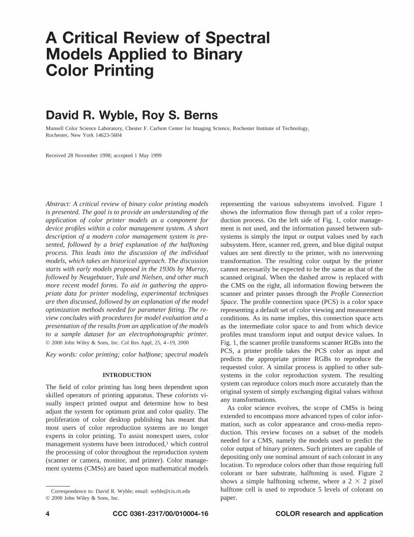
representing the various subsystems involved. Figure 1shows the information flow through part of a color repro-duction process. On the left side of Fig. 1, color manage-ment is not used, and the information passed between sub-systems is simply the input or output values used by eachsubsystem. Here, scanner red, green, and blue digital outputvalues are sent directly to the printer, with no interveningtransformation. The resulting color output by the printercannot necessarily be expected to be the same as that of thescanned original. When the dashed arrow is replaced withthe CMS on the right, all information flowing between thescanner and printer passes through theProfile ConnectionSpace. The profile connection space (PCS) is a color spacerepresenting a default set of color viewing and measurementconditions. As its name implies, this connection space actsas the intermediate color space to and from which deviceprofiles must transform input and output device values. InFig. 1, the scanner profile transforms scanner RGBs into thePCS, a printer profile takes the PCS color as input andpredicts the appropriate printer RGBs to reproduce therequested color. A similar process is applied to other sub-systems in the color reproduction system. The resultingsystem can reproduce colors much more accurately than theoriginal system of simply exchanging digital values withoutany transformations.

As color science evolves, the scope of CMSs is beingextended to encompass more advanced types of color infor-mation, such as color appearance and cross-media repro-duction. This review focuses on a subset of the modelsneeded for a CMS, namely the models used to predict thecolor output of binary printers. Such printers are capable ofdepositing only one nominal amount of each colorant in anylocation. To reproduce colors other than those requiring fullcolorant or bare substrate, halftoning is used. Figure 2shows a simple halftoning scheme, where a 23 2 pixelhalftone cell is used to reproduce 5 levels of colorant onpaper.

Correspondence to: David R. Wyble; email: [email protected]© 2000 John Wiley & Sons, Inc.

4 CCC 0361-2317/00/010004-16 COLOR research and application

The input to the halftoning process is a grayscale image.Each pixel in this image consists of at least three values:cyan, magenta, and yellow, and often a fourth colorant,black. These values, representing an amount of each respec-tive colorant, vary between 0–100%. In Fig. 2, the halftonecell is a group of four pixels. Any cell for which the inputvalue exceeds the threshold is imaged; cells falling belowthe threshold are not. By applying the halftoning process,the number of effective colorant levels is increased from 2to 5. Note that there is a corresponding decrease in imageresolution. After halftoning with the sample halftoning

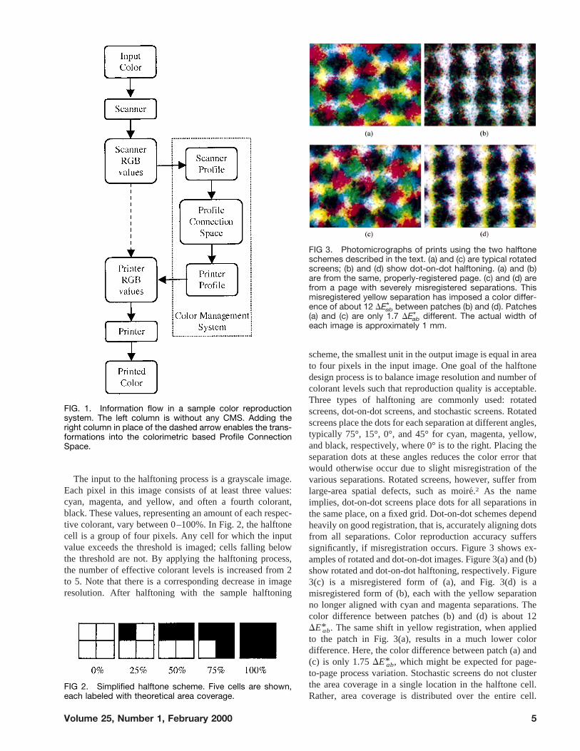
scheme, the smallest unit in the output image is equal in areato four pixels in the input image. One goal of the halftonedesign process is to balance image resolution and number ofcolorant levels such that reproduction quality is acceptable.Three types of halftoning are commonly used: rotatedscreens, dot-on-dot screens, and stochastic screens. Rotatedscreens place the dots for each separation at different angles,typically 75°, 15°, 0°, and 45° for cyan, magenta, yellow,and black, respectively, where 0° is to the right. Placing theseparation dots at these angles reduces the color error thatwould otherwise occur due to slight misregistration of thevarious separations. Rotated screens, however, suffer fromlarge-area spatial defects, such as moire´.2 As the nameimplies, dot-on-dot screens place dots for all separations inthe same place, on a fixed grid. Dot-on-dot schemes dependheavily on good registration, that is, accurately aligning dotsfrom all separations. Color reproduction accuracy sufferssignificantly, if misregistration occurs. Figure 3 shows ex-amples of rotated and dot-on-dot images. Figure 3(a) and (b)show rotated and dot-on-dot halftoning, respectively. Figure3(c) is a misregistered form of (a), and Fig. 3(d) is amisregistered form of (b), each with the yellow separationno longer aligned with cyan and magenta separations. Thecolor difference between patches (b) and (d) is about 12DE*ab. The same shift in yellow registration, when appliedto the patch in Fig. 3(a), results in a much lower colordifference. Here, the color difference between patch (a) and(c) is only 1.75DE*ab, which might be expected for page-to-page process variation. Stochastic screens do not clusterthe area coverage in a single location in the halftone cell.Rather, area coverage is distributed over the entire cell.

FIG. 1. Information flow in a sample color reproductionsystem. The left column is without any CMS. Adding theright column in place of the dashed arrow enables the trans-formations into the colorimetric based Profile ConnectionSpace.

FIG 2. Simplified halftone scheme. Five cells are shown,each labeled with theoretical area coverage.

FIG 3. Photomicrographs of prints using the two halftoneschemes described in the text. (a) and (c) are typical rotatedscreens; (b) and (d) show dot-on-dot halftoning. (a) and (b)are from the same, properly-registered page. (c) and (d) arefrom a page with severely misregistered separations. Thismisregistered yellow separation has imposed a color differ-ence of about 12 DE*ab between patches (b) and (d). Patches(a) and (c) are only 1.7 DE*ab different. The actual width ofeach image is approximately 1 mm.

Volume 25, Number 1, February 2000 5

Compared to the other halftoning methods, stochasticscreens are relatively new, and the older models presentedhere were not generally intended for such imaging systems.For more specific details of halftoning see, for example,Fink2 or Kang.3

Many models have been proposed to predict the coloroutput of binary printers. These date to the 1930s and havebeen refined many times over the subsequent decades. Thisarticle is not intended as a complete review of every modelever proposed. Rather, an historical approach starts withearly models and tracks their evolution. The models de-scribed here are selected, because they have been applied inmany contexts over the years and most have been used withsome success. Most of these models share a common “lin-eage” to the original Murray–Davies model, described be-low. For all models, a spectral form is used. The goal ofthese models is to predict thespectraloutput of the printer,as opposed to thecolor. This is to avoid metameric matchesby predicting physical printer performance (the reflectancespectrum), not perceptual output (the color). Model perfor-mance should be reported in the form of RMS spectraldifference and color difference inDE*ab. Both metricsshould be reported, because a large spectral difference maycorrespond to small color error. Note that if spectral outputis needed, spectral input data are also required.

REVIEW OF MODELS FOR HALFTONE COLORREPRODUCTION

Printers are typically characterized by printing and measur-ing a variety of samples, and determining model coeffi-cients, which predict physical properties of the output. Theresulting model predicts spectral reflectance or color giventhe cyan, magenta, and yellow input values. A model thusderived is aforward model, where inputs are RGB or CMYlevels, and outputs are in color coordinates: CIEXYZ,CIELAB, or another color space. The more useful modelform is theinversemodel, where the CMY printer requestsare predicted from color coordinates. This is the formneeded for the printer device profile, the input of which isthe color request given in profile connection space coordi-nates. The printer profile can then determine print CMYvalues that best reproduce the color request. At one time,inverting a device model was a critical operation, and ana-lytical forms needed to be chosen that could be inverted.Modern computing power and algorithm design make theuse of a lookup table (LUT) practical. This table is popu-lated by repeated runs of the forward model, and the inversemodel is accomplished by interpolation. Interpolation isrequired, because the input to the device profile is a grid incolor space, but the forward model generates a grid indevice input values (e.g., CMY values in the case of aprinter). The interpolation determines the device values thatbest reproduce the input color. Usually, this means deter-mining the point on the grid that is nearest the input color.For color applications, the LUT required is multidimen-sional, and is often referred to as a CLUT (color lookuptable). The use of a CLUT relaxes the mathematical con-

straints on the choice of forward models, freeing the mod-eler from the need to select an analytical form that isinvertable. The complete description of the methods ofCLUT creation or other methods of model inversion isbeyond the scope of this review. More details and an ex-panded list of references can be found in Ref. 3

Models described here are limited to three colorants.Most are not difficult to extend to four-colorant printers.The chief complication is that the CLUT is now four-dimensional. The details of four-color models and theirimplementation can also be found in Ref. 3

What follows is an historical description of the develop-ment of certain halftone printer models. Due to the reasonscited above, emphasis is only on the creation of an accurateforward model. It is assumed that the inverse models can beimplemented via multidimensional interpolation, and mod-els are not evaluated for their ability to be inverted.

Model Overview

Models presented are of two general types. Most areregression-basedmodels. These tend to be relatively sim-ple, with parameters fit to a set of data. They are often usefulfor modeling printer output, because they tend to be reason-ably accurate and their simplicity allows for short calcula-tion times. Regression-based models do not necessarilystrive for modeling of the physics of the process, but ratherto emulate the behavior of the system. More physicallyplausible forms, calledfirst-principals models, attempt tosimulate the physical process. It is hoped that these modelsaccurately estimate printer behavior, but a more importantuse is to increase understanding of the physical processitself. Often, the first-principals modeling approach cannotpredict printer output as well as the simpler models. How-ever, systematic trends should be apparent in the first-principals forms, even though the printer output might notbe predicted with absolute accuracy. Also, variation of theparameters should produce output that assists in the quali-tative description and understanding of the system.

REGRESSION BASED MODELS

Murray–Davies Model

Murray4 first published a simple model to predict outputdensity from input dot area. This model was originallyproposed privately by a colleague of Murray at the FranklinInstitute, E. R. Davies. Indeed, Murray himself refers to it as“Davies’ formula.” Instrumentation limitations at the timerequired Murray to work in density. The spectral reflectanceform is presented here:

Rl 5 atRl,t 1 ~1 2 at! Rl,s, (1)

where Rl is predicted spectral reflectance,at is fractionaldot area of the ink (thetint), Rl,t is the spectral reflectanceof the ink at full coverage, andRl,s is the spectral reflectanceof the substrate. Thel subscripts indicate all three reflec-tance values are a function of wavelength. Note how few

6 COLOR research and application

measurements need to be made for this model: only thespectral reflectance of the solid ink and that of the baresubstrate. The difficulty comes in estimating the area cov-erageat. Without an accurate understanding of the actualcolorant coverage, this model diverges unacceptably frommeasured data.

Some distinction must be made about various types of dotareas.Theoretical dot area(or equivalentlytheoretical areacoverage) is calculated from the actual binary image sent tothe printer. While not always physically reasonable, asquare pixel shape is assumed, and theoretical area coverageis determined as shown by the percentages in Fig. 2. (Pap-pas5 presented an in-depth analysis of circular pixel shapesand the implications of overlaps between pixels of the sameand differing separations.)Effective dot area(or effectivearea coverage) is always an estimated value. For example,if the spectral reflectance is accurately predicted by a par-ticular area coverage, this is referred to as the effective areacoverage,aeff. This is equivalent to selecting the best pro-portion to scaleRl,t such that it most closely matches themeasured spectral reflectance at area coverageat.

Use of the Murray–Davies model requires making thefundamental assumption that both the substrate and the inkare of uniform color. It is important to note that this is rarelythe case. For typical lithographic printing on plain paper,dot densities are not uniform. Nevertheless, these assump-tions apply to all the early models presented.

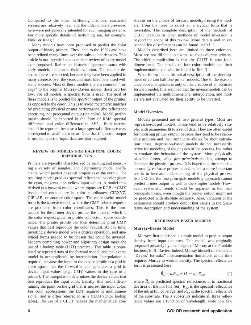
The Murray–Davies model makes a good deal of intuitivesense. From a conservation of energy viewpoint, the overallreflectance should be equal to the sum of the various com-ponents of light reflected off the print. If the light from eacharea is accounted for, the model should work well. How-ever, if the theoretical dot area (that is, the printer inputvalue) is used asat in Eq. (1), predicted reflectance forhalftoned images is consistently higher than measured re-flectance, as shown in Fig. 4. This effect is calleddot gain,the phenomenon whereby measured prints are alwaysdarker than predicted; the dots behave as if they are largerthan they are, hence dot gain.

The literature generally distinguishes between two typesof dot gain.Physical dot gainis actual growth in colorant

coverage due to the printing process. For example, whenapplying a drop of ink to a substrate, the drop might spreadin flight or upon contact with the substrate. Ink also spreadsupon penetrating the substrate. In these cases, the colorantcovers more area than originally intended. Alternatively,optical dot gainis the scattering of light in the substrate.Here, light that enters bare substrate may be scattered, andexit underneath a dot. Likewise, light entering through a dotmight be scattered and exit through bare substrate. Thesescattering effects cause the bare substrate to appear darkerthan expected, and the ink dots to appear lighter thanexpected. The overall effect is a darker image.

Estimating Effective Dot AreaAnother use of the Mur-ray–Davies model is to predict theeffective dot area. Ef-fective dot area is found by rearranging Eq. 1, into

aeff 5Rl5min,meas2 Rl5min,s

Rl5min,t 2 Rl2min,s. (2)

Note that Rl is replaced by the measured reflectance,Rl5min,meas, and the calculatedaeff replaces the input,at. Allreflectance values are subscriptedl 5 min to signify thatthis is not a spectral calculation, but one performed at asingle wavelength. The choice ofl is typically that of theminimum reflectance for either the measured or predictedtint. (This is the optimum wavelength, because it varies themost when dot area is changed.) In essence,aeff is the factorby which the solid ink reflectance should be scaled to equalthe measured reflectance of the sample. This equation canbe used to estimate dot gain, improving the estimation ofarea coverage. To extend Eq. (2) to a spectral form,aeff mustbe determined by a matrix calculation using least squaresanalysis:

aeff 5 Rmeas,adjRt,adjT (Rt,adjRt,adj

T )21. (3)

Reflectance terms in Eq. (3) are row vectors, the length ofwhich is the number of wavelengths in the spectral mea-surement. Here,Rmeas,adj 5 Rmeas 2 Rs, and Rt,adj 5Rt 2 Rs, and the supersciptsT and 21 indicate matrixtranspose and inverse, respectively. This calculation needsto be repeated for each patch in the separation ramp. Notethat this calculation assumes that thecmyarea coverages areindependent. Using Eq. (3), dot gain can be defined as thedeparture of effective dot area from the theoretical dot area,or aeff 2 at. This is a reasonable definition, because theMurray–Davies model is theoretically, if not practically,sound. If dot gain were known, and, hence,aeff could becalculated, monochrome printer output reflectance could bepredicted well by usingaeff asat in Eq. (1).

The calculation of effective area coverage, shown in Eq.(3) represents the first stage of all subsequent models. Theuse of aeff as input to later model stages is much morepractical than simply using printer input CMY digitalcounts. Effective area coverage is shown for the cyan sep-aration in Fig. 5. The calculated values can be stored, andused as input to more complex models by way of a one-dimensional LUT. Another possibility is to model the ef-fective area coverages. Figure 5 also shows a simple cubic

FIG 4. Predicted and measured spectral reflectance for50% theoretical area coverage. Predicted data were madeusing the Murray–Davies model in Eq. (1) with theoreticalarea coverage .


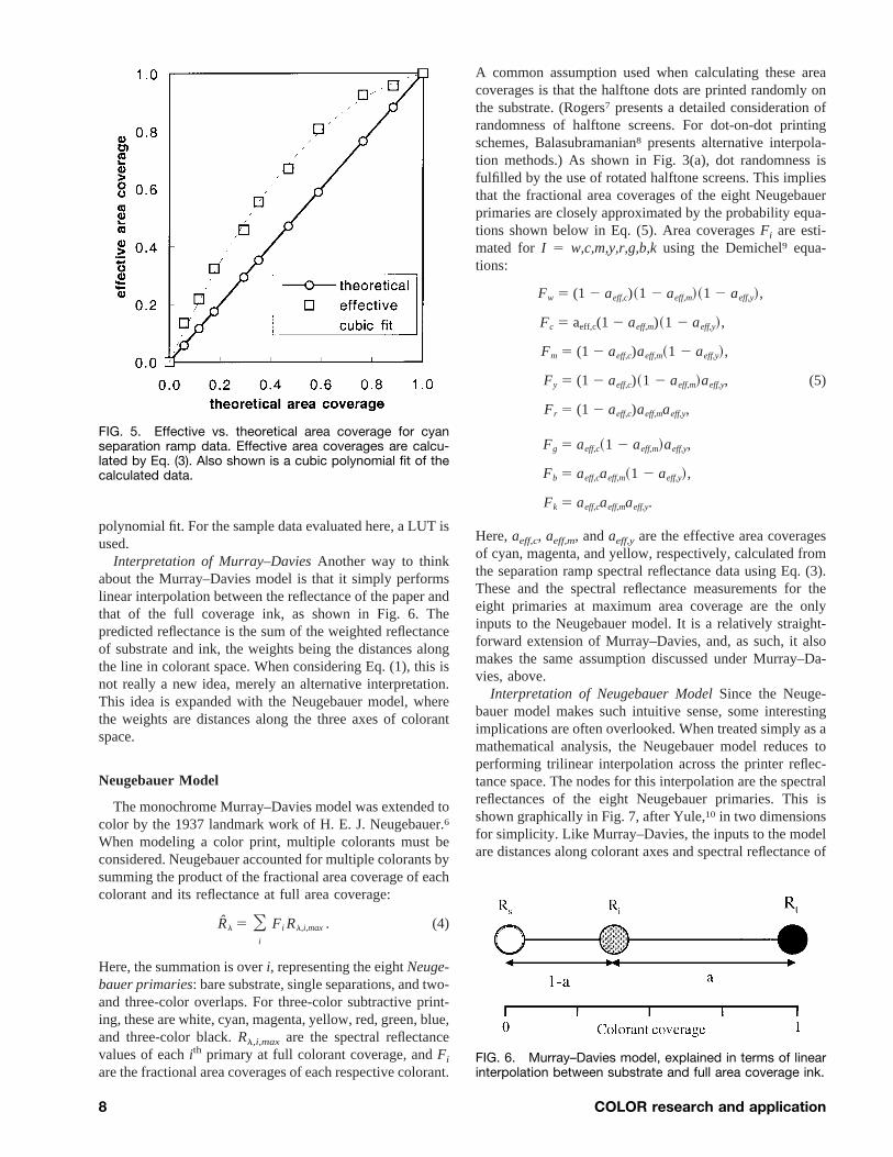
polynomial fit. For the sample data evaluated here, a LUT isused.

Interpretation of Murray–DaviesAnother way to thinkabout the Murray–Davies model is that it simply performslinear interpolation between the reflectance of the paper andthat of the full coverage ink, as shown in Fig. 6. Thepredicted reflectance is the sum of the weighted reflectanceof substrate and ink, the weights being the distances alongthe line in colorant space. When considering Eq. (1), this isnot really a new idea, merely an alternative interpretation.This idea is expanded with the Neugebauer model, wherethe weights are distances along the three axes of colorantspace.

Neugebauer Model

The monochrome Murray–Davies model was extended tocolor by the 1937 landmark work of H. E. J. Neugebauer.6

When modeling a color print, multiple colorants must beconsidered. Neugebauer accounted for multiple colorants bysumming the product of the fractional area coverage of eachcolorant and its reflectance at full area coverage:

Rl 5 Oi

Fi Rl,i,max. (4)

Here, the summation is overi, representing the eightNeuge-bauer primaries: bare substrate, single separations, and two-and three-color overlaps. For three-color subtractive print-ing, these are white, cyan, magenta, yellow, red, green, blue,and three-color black.Rl,i,max are the spectral reflectancevalues of eachith primary at full colorant coverage, andFi

are the fractional area coverages of each respective colorant.

A common assumption used when calculating these areacoverages is that the halftone dots are printed randomly onthe substrate. (Rogers7 presents a detailed consideration ofrandomness of halftone screens. For dot-on-dot printingschemes, Balasubramanian8 presents alternative interpola-tion methods.) As shown in Fig. 3(a), dot randomness isfulfilled by the use of rotated halftone screens. This impliesthat the fractional area coverages of the eight Neugebauerprimaries are closely approximated by the probability equa-tions shown below in Eq. (5). Area coveragesFi are esti-mated for I 5 w,c,m,y,r,g,b,kusing the Demichel9 equa-tions:

Fw 5 (1 2 aeff,c)~1 2 aeff,m!~1 2 aeff,y!,

Fc 5 aeff,c(1 2 aeff,m)~1 2 aeff,y!,

Fm 5 (1 2 aeff,c)aeff,m~1 2 aeff,y!,

Fy 5 (1 2 aeff,c)~1 2 aeff,m!aeff,y, (5)

Fr 5 (1 2 aeff,c)aeff,maeff,y,

Fg 5 aeff,c~1 2 aeff,m!aeff,y,

Fb 5 aeff,caeff,m~1 2 aeff,y!,

Fk 5 aeff,caeff,maeff,y.

Here,aeff,c, aeff,m, andaeff,y are the effective area coveragesof cyan, magenta, and yellow, respectively, calculated fromthe separation ramp spectral reflectance data using Eq. (3).These and the spectral reflectance measurements for theeight primaries at maximum area coverage are the onlyinputs to the Neugebauer model. It is a relatively straight-forward extension of Murray–Davies, and, as such, it alsomakes the same assumption discussed under Murray–Da-vies, above.

Interpretation of Neugebauer ModelSince the Neuge-bauer model makes such intuitive sense, some interestingimplications are often overlooked. When treated simply as amathematical analysis, the Neugebauer model reduces toperforming trilinear interpolation across the printer reflec-tance space. The nodes for this interpolation are the spectralreflectances of the eight Neugebauer primaries. This isshown graphically in Fig. 7, after Yule,10 in two dimensionsfor simplicity. Like Murray–Davies, the inputs to the modelare distances along colorant axes and spectral reflectance of

FIG. 6. Murray–Davies model, explained in terms of linearinterpolation between substrate and full area coverage ink.

FIG. 5. Effective vs. theoretical area coverage for cyanseparation ramp data. Effective area coverages are calcu-lated by Eq. (3). Also shown is a cubic polynomial fit of thecalculated data.


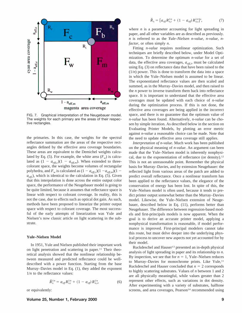
the primaries. In this case, the weights for the spectralreflectance summation are the areas of the respective rect-angles defined by the effective area coverage boundaries.These areas are equivalent to the Demichel weights calcu-lated by Eq. (5). For example, the white area (Fw) is calcu-lated as (12 aeff,c)(1 2 aeff,m). When extended to three-colorant space, the weights become volumes of rectangularpolyhedra, andFw is calculated as (12 aeff,c)(1 2aeff,m)(1 2aeff,), which is identical to the calculation in Eq. (5). Giventhat this interpolation is done across the entire output colorspace, the performance of the Neugebauer model is going tobe quite limited, because it assumes that reflectance space islinear with respect to colorant coverage. In reality, this isnot the case, due to effects such as optical dot gain. As such,methods have been proposed to linearize the printer outputspace with respect to colorant coverage. The most success-ful of the early attempts of linearization was Yule andNielsen’s now classic article on light scattering in the sub-strate.

Yule–Nielsen Model

In 1951, Yule and Nielsen published their important workon light penetration and scattering in paper.11 Their theo-retical analysis showed that the nonlinear relationship be-tween measured and predicted reflectance could be well-described with a power function. Starting from the baseMurray–Davies model in Eq. (1), they added the exponent1/n to the reflectance values:

Rl1/n 5 aeffRl,t

1/n 1 ~1 2 aeff! Rl,s1/n, (6)

or equivalently:

Rl 5 @aeffRl,t1/n 1 ~1 2 aeff! Rl,s

1/n#n, (7)

where n is a parameter accounting for light spreading inpaper, and all other variables are as described as previously.n is referred to as theYule–Nielsen n-value, n-value, n-factor, or often simplyn.

Fitting n-value requires nonlinear optimization. Suchtechniques are briefly described below, under Model Opti-mization. To determine the optimumn-value for a set ofdata, the effective area coverages,aeff,i, must be calculatedusing Eq. (3) on reflectance data that have been raised to the(1/n) power. This is done to transform the data into a spacein which the Yule–Nielsen model is assumed to be linear.The exponentiated reflectance values are then scaled andsummed, as in the Murray–Davies model, and then raised tothen power to inverse transform them back into reflectancespace. It is important to understand that the effective areacoverages must be updated with each choice ofn-valueduring the optimization process. If this is not done, theeffective area coverages are being applied in the incorrectspace, and there is no guarantee that the optimum value ofn-valuehas been found. Alternatively,n-valuecan be cho-sen by simple iteration. As described below in the section onEvaluating Printer Models, by plotting an error metricagainstn-valuea reasonable choice can be made. Note thatthe need to update effective area coverage still applies.

Interpretation of n-value.Much work has been publishedon the physical meaning ofn-value. An argument can beenmade that the Yule–Nielsen model is inherently nonphysi-cal, due to the exponentiation of reflectance (or density).12

This is not an unreasonable point. Remember the physicalbasis for Murray–Davies, and by extension Neugebauer: thereflected light from various areas of the patch are added topredict overall reflectance. Once a nonlinear transform hasbeen applied to the reflectance values, the elegance of theconservation of energy has been lost. In spite of this, theYule–Nielsen model is often used, because it tends to pre-dict printer output somewhat better than the Murray–Daviesmodel. Likewise, the Yule–Nielsen extension of Neuge-bauer, described below in Eq. (11), performs better thanNeugebauer. The difference between regression-based mod-els and first-principals models is now apparent. When thegoal is to derive an accurate printer model, applying anonphysical transformation is reasonable, if model perfor-mance is improved. First-principal modelers cannot takethis route, but must delve deeper into the underlying phys-ical process to uncover new aspects not yet accounted for bytheir model.

Ruckdeschel and Hauser13 presented an in-depth physicalanalysis of light spreading in paper and its relationship ton.By inspection, we see that forn 5 1, Yule–Nielsen reducesto Murray–Davies for monochrome prints. Like Yule,11

Ruckdeschel and Hauser concluded thatn 5 2 correspondsto highly scattering substrates. Values ofn between 1 and 2are all physically meaningful, while values greater than 2represent other effects, such as variations in dot density.After experimenting with a variety of substrates, halftonescreens, and area coverages, Pearson14 recommended using

FIG. 7. Graphical interpretation of the Neugebauer model.The weights for each primary are the areas of their respec-tive rectangles.


n 5 1.7, unless a better choice is known. Pearson also notedthat usingn 5 1.7 always improves performance overn 51. While both of these analyses are sound, is must be notedthat values ofn greater than 2 are often required for modern,high-resolution printers.

Another interesting interpretation ofn was made by Shi-raiwa and Mizuno.15 Their data were fit well byn of 3.0.Once an integer value ofn is assumed, additional mathe-matical expansions can be done that further clarify the roleof n in printer models. Suppose that the single separationcase is studied, e.g., Eq. (7) withn 5 2. For this analysis,Rl,t, the tint reflectance, is replaced by the productRl,sTl,i

2 ,whereRl,s is paper reflectance andTl,i is ink transmittance.Equation (7) becomes:

Rl 5 @aeff,i ~Rl,sTl,i2 !1/ 2 1 ~1 2 aeff,i! Rl,s

1/ 2#2, (8)

and the following expansion can be performed:

Rl 5 aeff,i2 Rl,sTl,i

2 1 2aeff,i ~1 2 aeff,i! Rl,s1/ 2Tl,i

1 ~1 2 aeff,i!2 Rl,s. (9)

The coefficients (areas) and color (reflectance) can bereadily seen in this expanded form. What can be learnedfrom this expansion is how the Yule–Nielsen modelchanges the predicted reflectance compared to the Murray–Davies model. There are intermediate terms correspondingto intermediate reflectances. In Eq. (9), the Murray–Daviesarea coverage for the primaries is reduced (since bothaeff,i

and 1 2 aeff,i are always less than 1), while adding areacoverage for theRl,s

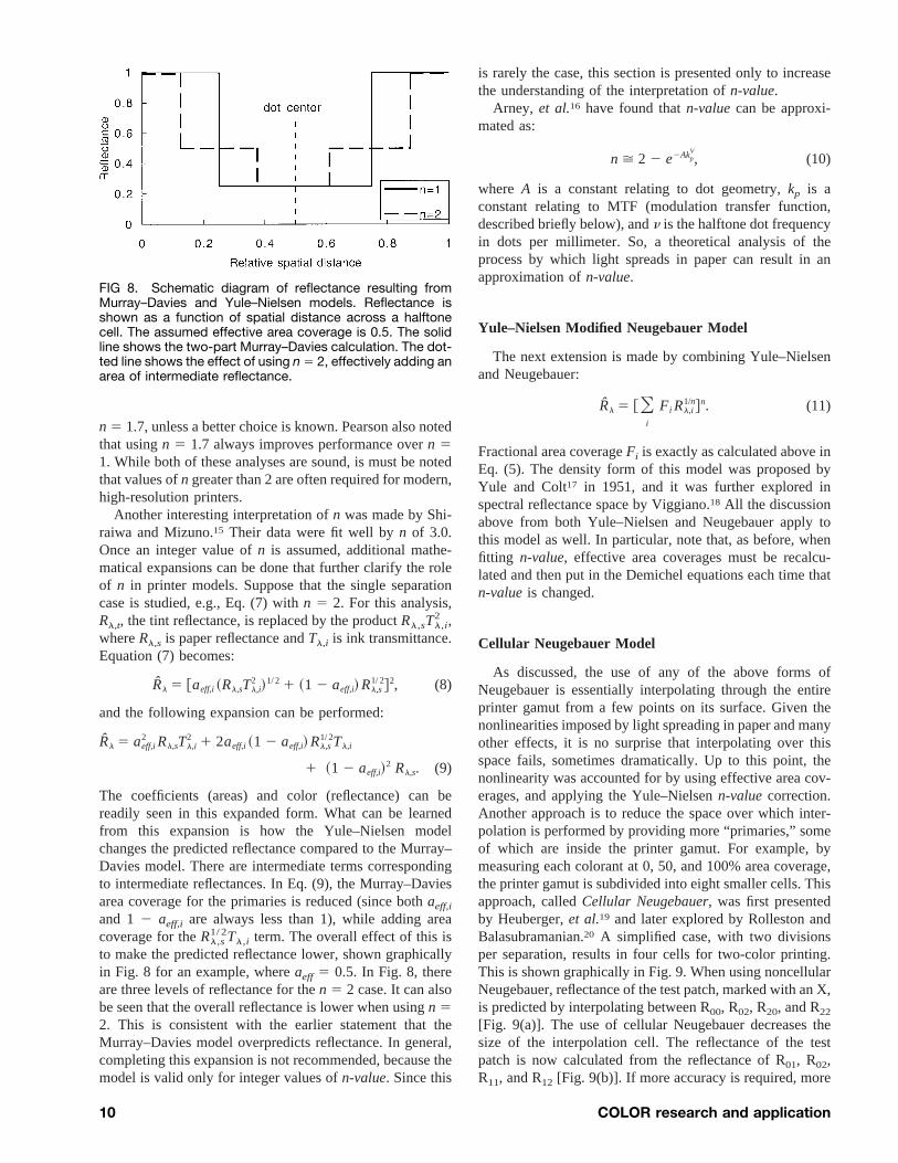
1/ 2Tl,i term. The overall effect of this isto make the predicted reflectance lower, shown graphicallyin Fig. 8 for an example, whereaeff 5 0.5. In Fig. 8, thereare three levels of reflectance for then 5 2 case. It can alsobe seen that the overall reflectance is lower when usingn 52. This is consistent with the earlier statement that theMurray–Davies model overpredicts reflectance. In general,completing this expansion is not recommended, because themodel is valid only for integer values ofn-value. Since this

is rarely the case, this section is presented only to increasethe understanding of the interpretation ofn-value.

Arney, et al.16 have found thatn-valuecan be approxi-mated as:

n > 2 2 e2AkpV

, (10)

where A is a constant relating to dot geometry,kp is aconstant relating to MTF (modulation transfer function,described briefly below), andn is the halftone dot frequencyin dots per millimeter. So, a theoretical analysis of theprocess by which light spreads in paper can result in anapproximation ofn-value.

Yule–Nielsen Modified Neugebauer Model

The next extension is made by combining Yule–Nielsenand Neugebauer:

Rl 5 @Oi

Fi Rl,i1/n#n. (11)

Fractional area coverageFi is exactly as calculated above inEq. (5). The density form of this model was proposed byYule and Colt17 in 1951, and it was further explored inspectral reflectance space by Viggiano.18 All the discussionabove from both Yule–Nielsen and Neugebauer apply tothis model as well. In particular, note that, as before, whenfitting n-value, effective area coverages must be recalcu-lated and then put in the Demichel equations each time thatn-valueis changed.

Cellular Neugebauer Model

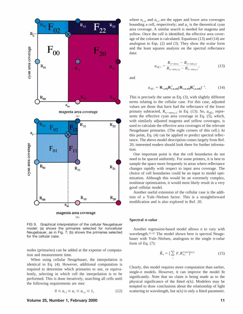
As discussed, the use of any of the above forms ofNeugebauer is essentially interpolating through the entireprinter gamut from a few points on its surface. Given thenonlinearities imposed by light spreading in paper and manyother effects, it is no surprise that interpolating over thisspace fails, sometimes dramatically. Up to this point, thenonlinearity was accounted for by using effective area cov-erages, and applying the Yule–Nielsenn-valuecorrection.Another approach is to reduce the space over which inter-polation is performed by providing more “primaries,” someof which are inside the printer gamut. For example, bymeasuring each colorant at 0, 50, and 100% area coverage,the printer gamut is subdivided into eight smaller cells. Thisapproach, calledCellular Neugebauer, was first presentedby Heuberger,et al.19 and later explored by Rolleston andBalasubramanian.20 A simplified case, with two divisionsper separation, results in four cells for two-color printing.This is shown graphically in Fig. 9. When using noncellularNeugebauer, reflectance of the test patch, marked with an X,is predicted by interpolating between R00, R02, R20, and R22

[Fig. 9(a)]. The use of cellular Neugebauer decreases thesize of the interpolation cell. The reflectance of the testpatch is now calculated from the reflectance of R01, R02,R11, and R12 [Fig. 9(b)]. If more accuracy is required, more

FIG 8. Schematic diagram of reflectance resulting fromMurray–Davies and Yule–Nielsen models. Reflectance isshown as a function of spatial distance across a halftonecell. The assumed effective area coverage is 0.5. The solidline shows the two-part Murray–Davies calculation. The dot-ted line shows the effect of using n 5 2, effectively adding anarea of intermediate reflectance.


nodes (primaries) can be added at the expense of computa-tion and measurement time.

When using cellular Neugebauer, the interpolation isidentical to Eq. (4). However, additional computation isrequired to determine which primaries to use, or equiva-lently, selecting in which cell the interpolation is to beperformed. This is done iteratively, searching all cells untilthe following requirements are met:

0 # ac,l # ac # ac,u # 1, (12)

whereac,u andac,l are the upper and lower area coveragesbounding a cell, respectively; andac is the theoretical cyanarea coverage. A similar search is needed for magenta andyellow. Once the cell is identified, the effective area cover-age of the colorant is calculated. Equations (13) and (14) areanalogous to Eqs. (2) and (3). They show the scalar formand the least squares analysis on the spectral reflectancedata:

aeff, c 5Rl5min,c 2 Rl5min,c,l

Rl5min,c,u 2 Rl5min,c,l, (13)

and

aeff,c 5 Rc,adjRc,u,adjT (Rc,u,adjRc,u,adj

T )21. (14)

This is precisely the same as Eq. (3), with slightly differentterms relating to the cellular case. For this case, adjustedvalues are those that have had the reflectance of the lowerprimary subtracted,Rl5min,c,l in Eq. (13). So,aeff,c repre-sents the effective cyan area coverage in Eq. (5), which,with similarly adjusted magenta and yellow coverages, isused to calculate the effective area coverages of the relevantNeugebauer primaries. (The eight corners of this cell.) Atthis point, Eq. (4) can be applied to predict spectral reflec-tance. The above model description comes largely from Ref.20; interested readers should look there for further informa-tion.

One important point is that the cell boundaries do notneed to be spaced uniformly. For some printers, it is best tosample the space more frequently in areas where reflectancechanges rapidly with respect to input area coverage. Thechoice of cell boundaries could be an input to model opti-mization. Although this would be an extremely complex,nonlinear optimization, it would most likely result in a verygood cellular model.

Another useful extension of the cellular case is the addi-tion of a Yule–Nielsen factor. This is a straightforwardmodification and is also explored in Ref. 20.

Spectral n-value

Another regression-based model allowsn to vary withwavelength.21,22 The model shown here is spectral Neuge-bauer with Yule–Nielsen, analogous to the singlen-valueform of Eq. (7):

Rl 5 @Oi

Fi Rl,i1/n~l!#n~l! (15)

Clearly, this model requires more computation than earlier,single-n models. However, it can improve the model fitsignificantly. Note that no claim is being made as to thephysical significance of the fittedn(l). Modelers may betempted to draw conclusions about the relationship of lightscattering to wavelength, butn(l) is only a fitted parameter.

FIG 9. Graphical interpretation of the cellular Neugebauermodel: (a) shows the primaries selected for noncellularNeugebauer, as in Fig. 7; (b) shows the primaries selectedfor the cellular case.


Regressing the Neugebauer Primaries

So far, models have focused on the nonlinear transfor-mation of the Neugebauer primaries, and linear regressionto determine the effective area coverage. Recent work hasbeen done by Balasubramanian,23 which also includes thefitting of the reflectance of the spectral primaries them-selves. This procedure can help avoid the measurementnoise that might be associated with the reflectance datarequired for previous models. However, to train the modelas described in Ref. 23, more input spectral reflectance datamust be measured than simply the eight primaries and theCMY ramps.

To implement this model, an iterative technique must beapplied. The author of the model recommends first using theleast squares method, described above, to determine theinitial choice of effective area coverages. The reflectance ofthe primaries is then determined by linear regression trans-formations using the input training set. Because the prima-ries have been changed, the effective area coverages mustbe found again, which may require another iteration to findnew primaries. In Ref. 23, only two iterations were neededfor a convergence.

FIRST PRINCIPALS MODELS

From this point, the models take fundamentally new forms.New methods are presented here: Arney, Engeldrum, andZeng;12 Arney, Wu, and Blehm;24 and Kruse and Wedin.25

The first attempts to increase the physical basis of Murray–Davies; this case is extended to color in the second. The lastis of a somewhat different spirit than all the previous mod-els. Up to now, ease of measurement and calculation havebeen important. Now, however, both data collection andmodel fitting are more difficult, in some cases relying ontheoretical rather than empirical parameters. This is to beexpected, because these models attempt to better account forphysical phenomena that have so far limited the perfor-mance of the simpler models. Also note that these modelssuffer somewhat in terms of absolute accuracy in theirprediction of printer output. While a decrease in accuracy isnever desired, it is acceptable in this case, because the chiefutility here is to learn about the physical process, not nec-essarily to derive a model suitable for a printer profile.Hence, these models are presented in an introductory formonly. Interested readers should seek the references for moredetailed information.

Expanded Murray–Davies Model

Arney, Engeldrum, and Zeng12 did not want to lose thephysical plausibility of the Murray–Davies model, but theywanted to make improvements to account for its knowndeficiencies. It was shown that the reflectance of paperbetween the halftone dots varied continuously as area cov-erage is increased.26 So, paper reflectance is not fixed, as theRs of the older models, but rather it is a function of areacoverage as well. It was also shown that dot reflectance is a

function of area coverage. The final form of the expandedMurray–Davies model is identical to Eq. (1). However,reflectance of the ink,Rl,t, and substrate,Rl,s, are functionsof area coveragesaeff,t, and aeff,s, respectively. The equa-tions for these functions are:

Rl,t 5 Rl,g@1 2 ~1 2 Tl, i!aeff,tw #@1 2 ~1 2 Tl, i!aeff,t

v #, (16)

and

Rl,s 5 Rl,g@1 2 ~1 2 Tl,i!~1 2 aeff,sw !#

3 @1 2 ~1 2 Tl,i!~1 2 aeff,sv !#. (17)

Several parameters are introduced here:Tl,i, the ink trans-mittance, is equal to (Rl,i/Rl,g)

1/2 at full area coverage;aeff,s,the effective area of the substrate, is 12 aeff,t; Rl,g is themeasured substrate reflectance; andw andv are empiricallyfit parameters. Note thatRl,g andTl,i serve similar functionsasRl,s andRl,t in Murray–Davies: they represent the influ-ence of the bare substrate and the ink at maximum areacoverage. This model is linear with reflectance, and does notuse the nonphysical exponentiation of reflectance. The pa-rameterv is intended to model softness of the dot edges.(According to the printer’s terminology, a “hard dot” is verysharp, with a clean distinction between dot edge and sub-strate; while soft dots are feathered, and ink thickness de-creases near their edges.)w represents the effect of lightscattering, as withn-value.

Extending to Color: the Probability Model

Just as the Murray–Davies model must be correct due toconservation of energy, so too should the Neugebauermodel work, if the correct reflectances of ink and paper canbe estimated. Arney, Wu, and Blehm24 reasoned that itshould be possible to determine the probability that lightwould enter and exit any given pair of color areas. In ourexamples, only cyan and magenta ink are considered; hence,there are four possible routes of entry into the paper andfour possible routes of egress. The four colors present arecyan, magenta, blue, and white. So, there are sixteen lightpaths that need to be considered. After deriving forms for allsixteen probabilities, the reflectance of the primaries can beestimated, and mixture reflectance can be calculated.

For this model description, the subscriptsi andj indicatethe color of the ink through which light leaves the paper,and the ink through which light enters the paper, respec-tively. First, the area coverages of the primaries are calcu-lated using Eq. (5), the Demichel probability equations.Pjj ,the probability that light will exit the same color area itentered, is calculated as:

Pjj 5 1 2 ~1 2 fj!@1 2 ~1 2 fj!w 1 ~1 2 fj

w!#, (18)

wherefi are the primary area coverages, andw is an empir-ically fit parameter. For light entering and exiting differentcolor areas, the probabilities are calculated using Eq. (19):

Pji 5 ~1 2 Pjj!S fi

1 2 fjD . (19)


The sixteen probabilities calculated above are essentiallyused as weights in a summation to determine the reflectanceof each primary. The primary ink reflectance is calculatedby

Rl,i 5 Rl,sTl,i Oj

STl, jPji

fj

fiD , (20)

where all terms are as previously defined. Recall that thesubscripti is where light leaves the paper, andj is wherelight enters the paper. Equation (20), then, simply sums thecolor of all the light that will exit the paper through colori,reflects this light off the substrateRs, and then filters it withtransmittanceTi on the way out. Once the reflectances of allprimaries are known, they can be used directly in Eq. (4),the original Neugebauer form.

Like Murray–Davies, this model retains a sense thatconservation of energy is obeyed. The model still requiresthe empirical exponentw, but a physical interpretation hasbeen made,24 relatingw to halftone geometry and substrateproperties. Because of its physical plausibility, this is auseful tool for exploring the complex process of the inter-action of light with ink and paper.

Modeling Paper Spread Function

Taking a step away from the Neugebauer and Yule–Nielsen forms, research has been published addressing thetheoretical physics of light scattering within the paper andthe dots.25–29 Also, attempts have been made to directlymeasure the paper spread function or paper MTF, the mod-ulation transfer function.30 (Here, paper spread function andMTF are treated together. Paper MTF is the paper spreadfunction after transformation into the frequency domain.Hence, either function can be derived from the other byprocessing with a forward or inverse Fourier transform.) Forthe purposes of this article, MTF can be considered theamount a binary input image is blurred by light spreading inthe paper. For example, a sharp edge between the substrateand ink is softened somewhat. Whether measuring or cal-culating the paper spread function, the result is applied tothe halftoned image in the form of a convolution:

Rx,y,l 5 @I x,y,lTx,y,l p Px,y,l#Tx,y,l, (21)

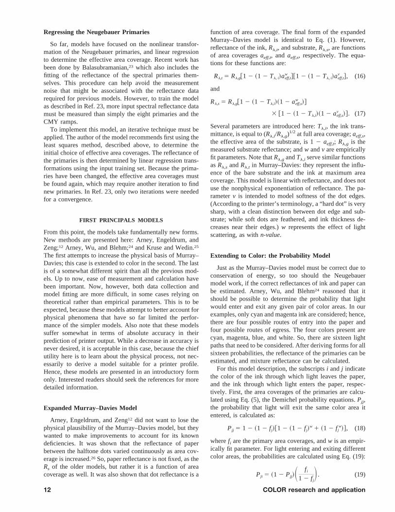
whereIx,y,l is the incident light, andPx,y,l is the point spreadfunction of the substrate, the mathematical description oflight spreading. Here, the predicted reflectance,Rx,y,l, andink transmittance,Tx,y,l, are both functions of spatial loca-tion, and, therefore, the halftone dots are no longer neces-sarily uniform. The desire to model nonuniform dots isshown graphically in Fig. 10. Here, there are two sets ofarrows, each depicting a ray of light. The arrows of eachpair pass through the same set of inks. For example, the pairof arrows on the left enter in through magenta and exit outthrough blue. These paths cannot be distinguished by theprobability model. It should be clear that the amount ofabsorption is going to be different for these two light paths,the solid arrow passing through much more cyan than the

dotted arrow. Similarly, the arrows on the right pass throughonly cyan, but very different amounts of cyan. This short-coming has been addressed by Rogers,31 who has proposeda method for incorporating an MTF-based model and theNeugebauer equations. Since the MTF model can accountfor nonuniform dots, it has a more physically plausiblebasis. This gain is made at the expense of greatly increasedcomputational complexity. When the MTF is empiricallycharacterized, measurement complexity increases signifi-cantly as well.

A more simplistic explanation of the color models can aidin the understanding of the MTF model. Consider thatNeugebauer attempts to predict spectral reflectance by usingthe eight Neugebauer primaries, which are combined invarying ratios to predict output spectral reflectance. Theprobability model increases the number of primaries to 64,and describes better the physics of the system. The MTFmodel, because of its use of convolution, has essentially aninfinite number of primaries. The nonuniform dots in mostprinting processes imply that an infinite number of prima-ries are present. The MTF model, therefore, best representsthe physical process. However, this should not be confusedwith the best model choice for a color management deviceprofile, which depends on many other factors, briefly de-scribed below.

EXPERIMENTAL TECHNIQUES

There are several important considerations to make regard-ing the creation and printing of a test target for fitting andverifying the models described here. This section is in-tended to provide guidelines to aid in creating appropriatedata to which these models can be applied.

Printer Description

One of the difficulties often encountered in deriving aprinter model is the lack of control over printer hardware.Printers often have built-inGray Component Replacement(GCR), where areas containing cyan, magenta, and yellowcolorant are replaced by black. For example, suppose that adark red patch is desired, consisting of exactly 20% cyan,50% magenta, and 50% yellow area coverage. In manyprinters, GCR is applied to these input values, resulting in aslightly different request sent to the actual printing hard-ware. In the example above, the printer software might

FIG.10. Justification of the need to model nonuniform dots.When applying the probability model, each pair of light pathsare treated the same.


choose a more efficient set of colorants to print, such as 20%black, 30% magenta, and 30% yellow area coverage. (Thisis more efficient, because total area coverage applied hasbeen reduced from 120% to 80%, out of a total of 400%possible for a four-color printer. We assume that the printercalibration is predicting that the observed color is the samein either case, so it makes economic sense to choose therequest resulting in less ink usage.) Other changes might bemade even if only a single colorant is requested. For exam-ple, printer software might be set up to automatically ac-count for dot gain, and input area coverages would beadjusted accordingly. While these limitations should notaffect the ability to derive a printer profile, when imple-menting a model it is most helpful to know actual areacoverage specifications sent to the imaging hardware.

Unfortunately, most modern printers do not allow theuser to bypass these internal control algorithms, making thejob of the modeler somewhat more difficult. The mostimportant concern is that it is usually impossible to guar-antee that no black is printed, requiring that the four-colorform of a model be implemented. This does complicatemodel derivation, but not so much as to make the processintractable for those willing to apply the statistical tech-niques described here.

Test Target Description

There are three main considerations in the design of thetest target: printer stability, separation registration, and re-quired test data. Printers are available in many technologies,and, therefore, have differing print-to-print and run-to-runstability. Likewise, separation registration (alignment) dif-fers among these various technologies. For all printers, theoptimal test data depends on the model selection. The de-scription that follows assumes that stability and registrationshould be monitored.

Each print should consist of three sections: controlpatches to assess stability, alignment cross-hairs to assessregistration, and sample patches. The size of the patchesdepends on the instrumentation used for the spectral mea-surement, described below. The control patches should besets of seven patches: cyan, magenta, yellow, red, green,blue, and three-color black. If within-print instability isexpected, the control patches should be placed on each endof the print. There should be alignment cross-hairs in twocorners of the print, one cross-hair each of red, blue, green,and black. Data patches can be placed in any fashion on theprint, but care should be used to not overburden the printerwith too high a total area coverage. For some technologies,this might affect process stability.

To monitor printer stability, the color of all controlpatches should be measured. Corresponding colors acrossmultiple prints are averaged, and the control values ofindividual prints are compared to this average. Dependingon the required accuracy, a threshold color differenceshould be set. Prints exceeding this threshold should bediscarded. Separation registration is evaluated by the align-ment cross-hairs. This can be done either visually or instru-

mentally. Note that the importance of registration dependsheavily on the halftoning scheme used, as discussed in theintroduction above.

The selection of test data is dependent on the choice ofmodels. In all cases, fitting effective area coverages requiresseveral levels in each separation ramp. The exact number oflevels depends on the number of levels in the halftone, butpracticality must enter the process as well. As a guide, eightto ten steps should be sufficient. There should be three orfour separation ramps, one for each colorant.

Other data to be printed are the Neugebauer primariesresulting from overlays, i.e., red, green, blue, and three-color black. For a four-color model, each of these, alongwith the cyan, magenta, and yellow primaries also need tobe combined with black, for a total of 16 primaries.

To verify the model, test data needs to be generated.Consideration needs to be paid to colors in the interior of theprinter gamut space. The ramp and primary data describedabove all lie on the gamut surface. A uniform sampling ofprinter space is useful to apply, such as 53 5 3 5 sampling,where each colorant is given 5 levels, and all 125 combi-nations are printed and measured. Note that some of themore complex models, in particular the cellular models,require such data for model fitting, and even more for propermodel verification.

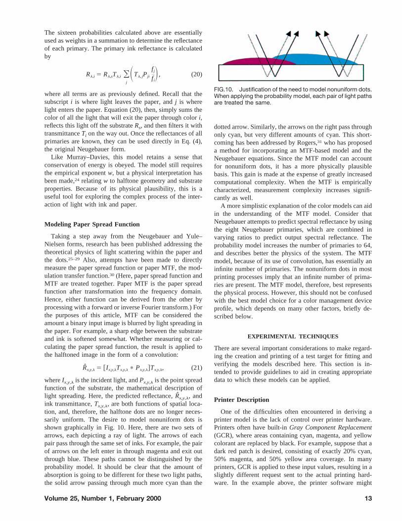
An example test target is shown in Fig. 11. Alignmentcross-hairs are in each corner, control patches are at the topand bottom, and samples patches are the large areas in thecenter. Sample patches are labeled with their respective

FIG. 11. Example test target, reduced.


cyan, magenta, and yellow digital values. Depending on thechoice of measurement device, the sample patches can bemade significantly smaller, thus fitting more per page andrequiring fewer overall pages to be printed. This is desir-able, because fewer pages means less opportunity for printervariability to impact the data. Data for the examples pre-sented here were measured on a large-area integratingsphere device, which required a sample area of at least 25mm in diameter.

Sample Measurement

The type of measurement depends both on the accuracydesired and the time needed for measurement. An auto-mated process is always useful, but not typically availablefor integrating sphere devices. For the best materials anal-ysis, integrating sphere, specular excluded (SPEX) shouldbe used. Since all the models here are spectral-based, spec-tral data need to be gathered. Typically, the wavelengthrange is 400–700 nm, at 10-nm intervals. A finer samplingmight improve the model performance, but 10 nm has beenused with success in many applications.

MODEL OPTIMIZATION

Optimization tools

There are several tools and techniques commonly usedfor optimizing the halftone models described here. All of themathematical analysis needed can be done in a spreadsheet,such as Microsoft Excelt. However, models requiringlarger datasets might find the spreadsheet application tooslow, and more specialized mathematical packages could beapplied, such as IDL™, from Research Systems Inc., orMatlab™, from The Math Works, Inc.

Optimization Techniques

As model forms have evolved, the complexity of theoptimization required has typically increased. Murray–Da-vies and Neugebauer require linear optimization to estimateeffective area coverage. The Yule–Nielsenn-valuerequiresnonlinear optimization, as does the extended Murray–Da-vies model. The cellular Neugebauer model could be usedwith only linear optimization, by arbitrarily choosing thecell boundaries, or with nonlinear optimization, using thetools to select cell boundaries. In both cases, linear optimi-zation is needed for estimating effective area coverages. Allthese types of optimizations can be done using any of thetools listed above. For a mathematical introduction to non-linear estimation techniques, see Ref. 32.

Optimization Objectives

The ultimate goal of these optimizations is to minimizethe spectral error of the models. Therefore, a useful objec-tive function is the root mean square (RMS) of the differ-ence between the measured and predicted spectral reflec-

tance. To retain the spirit of minimizing the measurementrequirements, fitting can be done against separation rampdata only. However, some of the models, e.g., cellular,require the measurement of much more data, and these tooshould be included in the model optimization.

EVALUATING PRINTER MODELS

Model Evaluation Technique

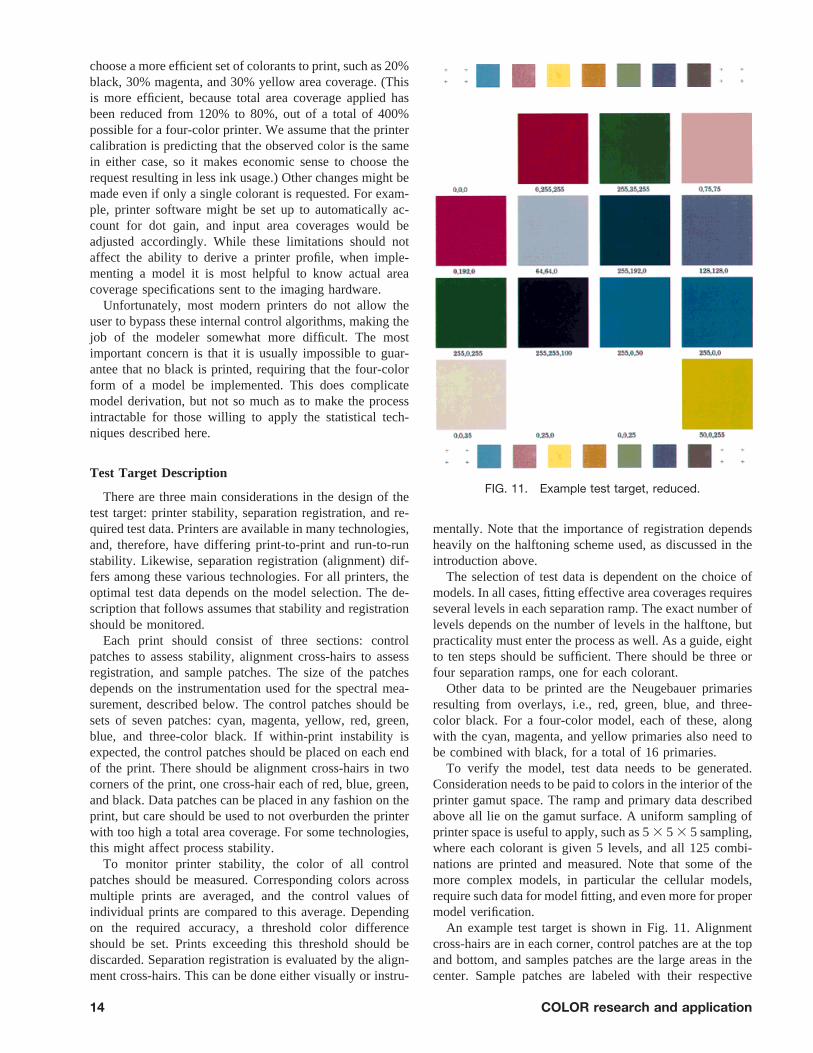
Nearly all the models presented above require relativelyfew measurements to be made. Of course, this means thatthe models must then perform some type of interpolation topredict printer output for input values not in the measureddataset. Since the focus here is on spectral-based models, itis important to examine the reflectance spectra of the mea-sured data. By viewing the data in this way, an intuitivesense can be gained as to the utility of the respectivemodels. Figure 12 shows the reflectance data for cyanseparation ramp data. The simplest model presented, Mur-ray–Davies, interpolates between the highest curve, for areacoverage of 0, and the lowest one, for area coverage of 1.0.Due to the great difference between reflectance of paper andthe solid area patches, it is difficult to interpret how wellthese data can predict the intermediate reflectance values ofcyan area coverage. Therefore, a normalized form of reflec-tance is used, after Berns,et al.33 The equation used fornormalizing cyan reflectance is:

Rl,normalized5Rl,c 2 Rl,w

~Rc 2 Rw!l5minimum(22)

where l 5 minimum corresponds to the wavelength atwhich full area coverage cyan reflectance is minimum.Similar forms are applied to magenta and yellow. Lookingat the normalized cyan reflectance data in Fig. 13, theaccuracy of the Murray–Davies interpolation can be visu-ally assessed more easily. For the Murray–Davies equationto hold, all these spectra would be coincident. Since this isobviously not the case, it is clear that some enhancementneeds to be made. (Note that for this and all the othernormalized spectral plots, there is no reason why valuescannot be greater than one or less than zero. This is simply

FIG. 12. Reflectance data from cyan separation ramps.


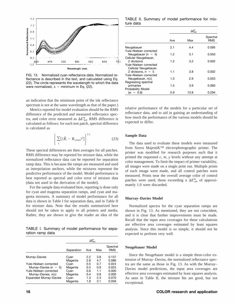
an indication that the minimum point of the ink reflectancespectrum is not at the same wavelength as that of the paper.)

Metrics reported for model evaluation should be the RMSdifference of the predicted and measured reflectance spec-tra, and color error measured asDE*94. RMS difference iscalculated as follows: for each test patch, spectral differenceis calculated as

H Ol

@~Ri 2 Ri,meas!2#J 1/ 2

(23)

These spectral differences are then averages for all patches.RMS difference may be reported for mixture data, while thenormalized reflectance data can be reported for separationramp data. This is because the ramps are measured and usedas interpolation anchors, while the mixtures represent thepredictive performance of the model. Model performance isbest reported as spectral and color error of mixture data(data not used in the derivation of the model).

For the sample data evaluated here, reporting is done onlyfor cyan and magenta separation ramps, and cyan and ma-genta mixtures. A summary of model performance for alldata is shown in Table I for separation data, and in Table IIfor mixture data. Note that the results summarized hereshould not be taken to apply to all printers and media.Rather, they are shown to give the reader an idea of the

relative performance of the models for a particular set ofreflectance data, and to aid in gaining an understanding ofhow much the performance of the various models should beexpected to differ.

Sample Data

The data used to evaluate these models were measuredfrom Xerox MajestiK™ electrophotographic printer. Theprinter was modified for research purposes such that itprinted the requestedc, m, y levels without any attempt atcolor management. To limit the impact of printer variability,all images were made on a single print run. Multiple printsof each image were made, and all control patches weremeasured. Prints near the overall average color of controlpatches were used; those exceeding aDE*ab of approxi-mately 1.0 were discarded.

Murray–Davies Model

Normalized spectra for the cyan separation ramps areshown in Fig. 13. As mentioned, they are not coincident,and it is clear that further improvements must be made.Recall that the input area coverages for these calculationsare effective area coverages estimated by least squaresanalysis. Since this model is so simple, it should not beexpected to perform very well.

Neugebauer Model

Since the Neugebauer model is a simple three-color ex-tension of Murray–Davies, the normalized reflectance spec-tra are the same as those in Fig. 13. As with the Murray–Davies model predictions, the input area coverages areeffective area coverages estimated by least squares analysis.As seen in Table II, the mixture fits are good, but notexceptional.

FIG. 13. Normalized cyan reflectance data. Normalized re-flectance is described in the text, and calculated using Eq.(22). The circle represents the wavelength to which the datawere normalized, l 5 minimum in Eq. (22).

TABLE I. Summary of model performance for sepa-ration ramp data

DE*94

Separation Ave MaxSpectral

RMS

Murray–Davies Cyan 2.2 3.8 0.137Magenta 2.8 4.7 0.086

Yule–Nielsen corrected Cyan 0.5 0.7 0.024Murray–Davies (n 5 5) Magenta 0.5 0.9 0.025

Yule–Nielsen corrected Cyan 0.6 1.1 0.000Murray–Davies, n(l) Magenta 0.4 0.8 0.000

Expanded Murray–Davies Cyan 1.3 2.3 0.070Magenta 1.8 3.1 0.058

TABLE II. Summary of model performance for mix-ture data

DE*94

Ave MaxSpectral

RMS

Neugebauer 2.1 4.4 0.095Yule–Nielsen corrected

Neugebauer (n 5 5) 1.2 3.1 0.050Cellular Neugebauer,

2 divisions 1.2 3.2 0.002Yule–Nielsen corrected

Cellular Neugebauer,2 divisions, n 5 5 1.1 3.8 0.002

Yule–Nielsen correctedNeugebauer, n(l) 1.3 2.9 0.053

Regressing spectralprimaries 1.5 3.9 0.060

Probability Model(w 5 0.8) 5.9 13.8 0.294


Yule–Nielsen Model

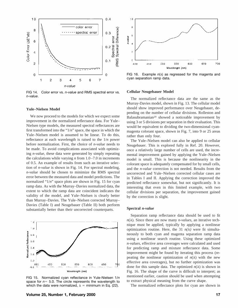
We now proceed to the models for which we expect someimprovement in the normalized reflectance data. For Yule–Nielsen type models, the measured spectral reflectances arefirst transformed into the “1/n” space, the space in which theYule–Nielsen model is assumed to be linear. To do this,reflectance at each wavelength is raised to the 1/n powerbefore normalization. First, the choice ofn-valueneeds tobe made. To avoid complications associated with optimiz-ing n-value, these data were generated by simply repeatingthe calculations while varyingn from 1.0–7.0 in incrementsof 0.5. An example of results from such an iterative selec-tion of n-valueis shown in Fig. 14. For spectral modeling,n-value should be chosen to minimize the RMS spectralerror between the measured data and model predictions. Thenormalized “1/n” space plots are shown in Fig. 15 for cyanramp data. As with the Murray–Davies normalized data, theextent to which the ramp data are coincident indicates thevalidity of the model, and Yule–Nielsen is clearly betterthan Murray–Davies. The Yule–Nielsen corrected Murray–Davies (Table I) and Neugebauer (Table II) both performsubstantially better than their uncorrected counterparts.

Cellular Neugebauer Model

The normalized reflectance data are the same as theMurray-Davies model, shown in Fig. 13. The cellular modelshould show improved performance over Neugebauer, de-pending on the number of cellular divisions. Rolleston andBalasubramanian20 showed a noticeable improvement byusing 3 or 5 divisions per separation in their evaluation. Thiswould be equivalent to dividing the two-dimensional cyan-magenta colorant space, shown in Fig. 7, into 9 or 25 areasrather than only four.

The Yule–Nielsen model can also be applied to cellularNeugebauer. This is explored fully in Ref. 20. However,once a relatively large number of cells are used, the incre-mental improvement gained by applying the Yule–Nielsenmodel is small. This is because the nonlinearity in thecolorant space is adequately compensated for by small cells,and then-valuecorrection is not needed. Results from theuncorrected and Yule–Nielsen corrected cellular cases arein Tables I and II. Applying the correction improved thepredicted reflectance somewhat, but not significantly. It isinteresting that even in this limited example, with twocellular divisions per separation, the improvement gainedby the correction is slight.

Spectral n-value

Separation ramp reflectance data should be used to fitn(l). Since there are now manyn-values, an iterative tech-nique must be applied, typically by applying a nonlinearoptimization routine. Here, the 31n(l) were fit simulta-neously to both cyan and magenta separation ramp datausing a nonlinear search routine. Using these optimizedn-values, effective area coverages were calculated and usedfor predicting ramp and mixture reflectance data. Someimprovement might be found by iterating this process (re-peating the nonlinear optimization ofn(l) with the neweffective area coverages), but no further optimization wasdone for this sample data. The optimizedn(l) is shown inFig. 16. The shape of the curve is difficult to interpret; asmentioned earlier, caution should be used when attemptingto extract physical meaning from the curve shape.

The normalized reflectance plots for cyan are shown in

FIG 14. Color error vs. n-value and RMS spectral error vs.n-value.

FIG 15. Normalized cyan reflectance in Yule-Nielsen 1/nspace for n5 5.0. The circle represents the wavelength towhich the data were normalized, l 5 minimum in Eq. (22).

FIG 16. Example n(l) as regressed for the magenta andcyan separation ramp data.


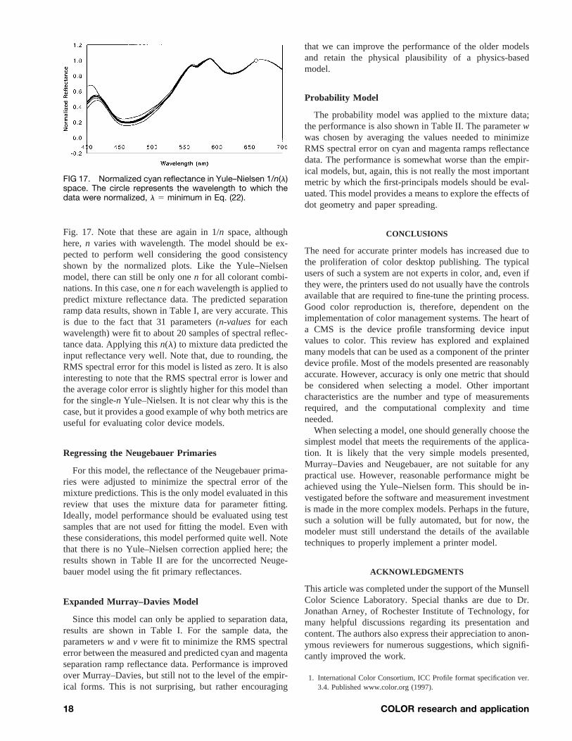
Fig. 17. Note that these are again in 1/n space, althoughhere,n varies with wavelength. The model should be ex-pected to perform well considering the good consistencyshown by the normalized plots. Like the Yule–Nielsenmodel, there can still be only onen for all colorant combi-nations. In this case, onen for each wavelength is applied topredict mixture reflectance data. The predicted separationramp data results, shown in Table I, are very accurate. Thisis due to the fact that 31 parameters (n-values for eachwavelength) were fit to about 20 samples of spectral reflec-tance data. Applying thisn(l) to mixture data predicted theinput reflectance very well. Note that, due to rounding, theRMS spectral error for this model is listed as zero. It is alsointeresting to note that the RMS spectral error is lower andthe average color error is slightly higher for this model thanfor the single-n Yule–Nielsen. It is not clear why this is thecase, but it provides a good example of why both metrics areuseful for evaluating color device models.

Regressing the Neugebauer Primaries

For this model, the reflectance of the Neugebauer prima-ries were adjusted to minimize the spectral error of themixture predictions. This is the only model evaluated in thisreview that uses the mixture data for parameter fitting.Ideally, model performance should be evaluated using testsamples that are not used for fitting the model. Even withthese considerations, this model performed quite well. Notethat there is no Yule–Nielsen correction applied here; theresults shown in Table II are for the uncorrected Neuge-bauer model using the fit primary reflectances.

Expanded Murray–Davies Model

Since this model can only be applied to separation data,results are shown in Table I. For the sample data, theparametersw andv were fit to minimize the RMS spectralerror between the measured and predicted cyan and magentaseparation ramp reflectance data. Performance is improvedover Murray–Davies, but still not to the level of the empir-ical forms. This is not surprising, but rather encouraging

that we can improve the performance of the older modelsand retain the physical plausibility of a physics-basedmodel.

Probability Model

The probability model was applied to the mixture data;the performance is also shown in Table II. The parameterwwas chosen by averaging the values needed to minimizeRMS spectral error on cyan and magenta ramps reflectancedata. The performance is somewhat worse than the empir-ical models, but, again, this is not really the most importantmetric by which the first-principals models should be eval-uated. This model provides a means to explore the effects ofdot geometry and paper spreading.

CONCLUSIONS

The need for accurate printer models has increased due tothe proliferation of color desktop publishing. The typicalusers of such a system are not experts in color, and, even ifthey were, the printers used do not usually have the controlsavailable that are required to fine-tune the printing process.Good color reproduction is, therefore, dependent on theimplementation of color management systems. The heart ofa CMS is the device profile transforming device inputvalues to color. This review has explored and explainedmany models that can be used as a component of the printerdevice profile. Most of the models presented are reasonablyaccurate. However, accuracy is only one metric that shouldbe considered when selecting a model. Other importantcharacteristics are the number and type of measurementsrequired, and the computational complexity and timeneeded.

When selecting a model, one should generally choose thesimplest model that meets the requirements of the applica-tion. It is likely that the very simple models presented,Murray–Davies and Neugebauer, are not suitable for anypractical use. However, reasonable performance might beachieved using the Yule–Nielsen form. This should be in-vestigated before the software and measurement investmentis made in the more complex models. Perhaps in the future,such a solution will be fully automated, but for now, themodeler must still understand the details of the availabletechniques to properly implement a printer model.

ACKNOWLEDGMENTS

This article was completed under the support of the MunsellColor Science Laboratory. Special thanks are due to Dr.Jonathan Arney, of Rochester Institute of Technology, formany helpful discussions regarding its presentation andcontent. The authors also express their appreciation to anon-ymous reviewers for numerous suggestions, which signifi-cantly improved the work.

1. International Color Consortium, ICC Profile format specification ver.3.4. Published www.color.org (1997).

FIG 17. Normalized cyan reflectance in Yule–Nielsen 1/n(l)space. The circle represents the wavelength to which thedata were normalized, l 5 minimum in Eq. (22).


2. Fink P. Postscript screening: Adobe accurate screens. Mountain View:Adobe; 1992.

3. Kang H. Color technology for electronic imaging devices. Bellingham,Washington: SPIE; 1996.

4. Murray A. Monochrome reproduction in photoengraving. J FranklinInst 1936;221:721–744.

5. Pappas TN. Model-based halftoning of color images. IEEE Trans ImProc 1997;6:1014–1024.

6. Neugebauer HEJ. Die theoretischen grundlagen des mehrfarbendrucks,Zeitscrift fur wissenschaftliche Photographie 1937;36:73–89 [Reprint-ed as Neugebauer memorial seminar on color reproduction, Proc SPIE1989;1184:194–202.]

7. Rogers GL. Neugebauer revisited: random dots in halftone screening.Col Res Appl 1998;23:104–113.

8. Balasubramanian R. A printer model for dot-on-dot halftone screens.Proc SPIE 1995;2413:356–364.

9. Demichel ME. Proce´de 1924;26:17–21, 26–27.10. Yule JAC. Principles of color reproduction. New York: Wiley; 1967.11. Yule JAC, Nielsen WJ. The penetration of light into paper and its

effect on halftone reproductions. TAGA Proc 1951;3:65–76.12. Arney JS, Engeldrum PG, Zeng H. An expanded Murray–Davies

model of tone reproduction in halftone imaging. J Imag Sci Tech1995;39:502–508.

13. Ruckdeschel FR, Hauser OG. Yule–Nielsen effect on printing: aphysical analysis. Appl Opt 1978;17:3376–3383.

14. Pearson M. n value for general conditions. TAGA Proc 1980;32:415–425.

15. Shiraiwa Y, Mizuna T. Equation to predict colors of halftone printsconsidering the optical properties of paper. J Imag Sci Tech 1993;37:385–391.

16. Arney JS, Arney CD, Katsube M, Engeldrum PG. The impact of paperoptical properties on hard copy image quality. Proc. IS&T Non-impactPrinting 12: Int Conf Digital Print Tech; 1996. p 166–168.

17. Yule JAC, Colt R. Colorimetric investigations in multicolor printing.TAGA Proc 1951;3:77–82.

18. Viggiano JAS. The color of halftone tints. TAGA Proc 1985;37:647–661.

19. Heuberger KJ, Jing ZM, Persiev S. Color transformations and lookuptables. TAGA/ISCC Proc; 1992. p 863–881.

20. Rolleston R, Balasubramanian R. Accuracy of various types of Neuge-bauer model. Proc IS&T SID Col Imag Conf; 1993. p 32–37.

21. Iino K, Berns RS. Building color management modules using linearoptimization I. Desktop color system. J Imag Sci Tech 1998;42:79–94.

22. Iino K, Berns RS. Building color management modules using linearoptimization II. Prepress system for offset printing. J Imag Sci Tech1997;42:99–114.

23. Balasubramanian R. The use of spectral regression in modeling colorhalftone printers. Rochester, NY: IS&T/OSA Optics Imag Info Age;1996.

24. Arney JS, Wu T, Blehm C. Modeling the Yule–Nielsen effect on colorhalftones. J Imag Sci Tech 1998;42:335–340.

25. Kruse B, Wedin M. A new approach to dot gain modeling. TAGA Proc1995;47:329–338.

26. Engeldrum PG. The color between the dots. J Imag Sci Tech 1994;38:545–551.

27. Gustavson S, Wedin M, Kruse B. 3D modeling of light diffusion inpaper. TAGA Proc 1995;47:848–855.

28. Rogers GL. Optical dot gain in a halftone print. J Imag Sci Tech1997;41:643–656.

29. Maltz M. Light scattering in xerographic images. J App Photo Tech1983;9:83–89.

30. Engeldrum PG, Pridham B. Application of turbid medium theory topaper spread function measurements. TAGA Proc 1995;47:336–352.

31. Rogers GL. Effect of light scatter on halftone color. J Opt Soc Am A1998;15:1831–1821.

32. Draper NR, Smith H. Applied regression analysis. New York: Wiley;1981.

33. Berns RS, Bose A, Tzeng DY. The spectral modeling of large-formatink-get printers. Munsell Color Science Laboratory Internal Report;1996.


Documents

A Critical Review of Spectral Models Applied to Binary …webstaff.itn.liu.se/~sasgo26/Digital_Halftoning...A Critical Review of Spectral Models Applied to Binary Color Printing David