A critique of the traditional presentation of thermodynamicsneo-classical-physics.info/.../3/6/34363841/born_-_thermodynamics.pdf · A critique of the traditional presentation of

“Kritische Betrachtungen zur traditionellen Darstellung der Thermodynamik,” Phys. Zeit. 22 (1921), 218-224.

A critique of the traditional presentation of thermodynamics

By. M. Born

Translated by D. H. Delphenich

_____

Introduction

The mathematical tools that the physicist needs in order to represent the classical domain of his science seem to be narrowly restricted in scope. Systems of partial differential equations dominated that period of physics which lies completely behind us today in this age of quantum physics. Furthermore, there is only a surprisingly small number of differential equations that present themselves repeatedly. Indeed, there is, e.g., no domain of continuum physics in which Poisson’s equation does not play a role. That fact, which is already conspicuous for the beginner, does not rest upon mere happenstance, but upon a principle of research that arises from economy of thought. The formulas that mathematics provides are there already, and indeed a relatively small number of them have been worked out to the extent that the physicist can then begin anything. Therefore, he will convert and manipulate his empirical material and the laws that he obtains from it until they take on a prearranged form. In classical physics, the logical treatment of a domain is first considered to be complete when it has been reduced to a chapter in “normal” mathematics. There is only one conspicuous exception: viz., classical thermodynamics. The methods that are usually applied in order to derive the basic laws in that discipline depart completely from the otherwise-customary methods. One already sees that in the fact that there is no other domain of physics in which arguments and conclusions are applied that have any similarity to the process of Carnot cycles. If one further asks which formulas and theorems of mathematics will actually be used for the thermodynamic inferences then one will hardly be able to characterize them as such. The physical theories whose presentation one should appeal to are so singular in their details that nothing seems to remain after one deducts that physical content. But that cannot be the case. Thermodynamics then culminates in a typical mathematical assertion, namely, the existence of a certain function of the state parameters – viz., entropy – and gives prescriptions for its calculation. One would have to admit that thermodynamics, in its traditional form, has still not realized the logical ideal of separating the physical content from the mathematical representation.

Born – A critique of the traditional presentation of thermodynamics 2

Therefore, in the year 1909, a treatise by C. Carathéodory (1) appeared that completely achieved that goal. That paper has been overlooked by the physics community almost entirely. That is partly based in the very abstract manner of representation that aimed for maximum generality and partly in where it was published: Most physicists would devote little attention to a treatise on thermodynamics that is published in Mathematischen Annalen and in which cyclic processes are not mentioned once, and yet it deserves to be read, not only to clarify the basic concepts, but also for the advantage that the new representation offers as far as teaching is concerned. In order to lighten the burden of studying Carathéodory’s treatise, I have made an attempt to present its basic ideas here in an entirely simple fashion and submit them to my colleagues. I know that thermodynamics exerts a strongly intellectual charm in the form that the old masters gave to it and is anchored very firmly in the consciousness of physicists. Perhaps the new foundations will nonetheless make some friends. If it also lacks those wonderful inroads that lead from the facts of experience to the fundamental laws in an almost-magical way then it is, in return, more transparent and appeals to simply the “normal” mathematics that everyone has learned. In what follows, I will seamlessly relate the train of thought that leads from the facts of experience to the mathematical formulas of the fundamental laws. Therefore, I will, however, treat the terms that coincide with the usual manner of representation only briefly and illuminate in detail only those points at which something new appears. Here, a certain critique of the classical method of proof must also be inserted. However, it shall by no means imply that I wish to diminish the magnificent achievements of the masters whose intuition has led the way, but only to remove some of the detritus that no one has dared to deal with up to now out of an excessively pious adherence to tradition.

§ 1. – Definitions.

We would like to confine our considerations to the simplest systems of all, namely, the ones that are composed of chemically-unchanging gases and fluids. However, our method can be adapted to completely-arbitrary systems of the kind that one prefers to consider in thermodynamics with no difficulty. We will come back to them briefly in the concluding remarks. We assume that the basic ideas of mechanics (such as volume, mass, force, pressure, etc.) are known, but not the thermal ones (such as temperature, amount of heat, etc.), since defining them rigorously is our goal. The intrinsic state of a fluid of given mass will be determined by purely mechanical considerations as long as its volume is known; the pressure is then a function of volume. However, the latter is not the case, in fact. One can change pressure at constant volume and conversely, namely, by those processes that one calls heating or cooling and which will be accompanied by the sensations of hotness or coldness. Now, the thermodynamic way of looking at things consists of introducing the volume V as something that varies independently of the pressure p. We shall assume that the intrinsic state of the body (fluid) is determined completely by being given V, p.

(1) C. Carathéodory, “Untersuchungen über die Grundlagen der Thermodynamik,” Math. Ann. 61 (1909), 355.


The individual bodies of that kind shall be separated from each other and from the outside by “walls” that we should not include among the bodies considered, although we shall make special idealizations about their behavior. Indeed, here we shall consider only two types of walls that have in common the fact that they are impermeable to matter. As is known, walls that are permeable to matter also play a significant role in theoretical thermochemistry, but allowing them would introduce no essential difficulties, and we will touch upon them only briefly in the concluding section. Hence, we shall restrict ourselves here to walls that are impermeable to heat (viz., adiabatic ones) and ones that are permeable to heat (viz., diathermal ones). However, since we have not introduced the concept of heat, we must also arrange that the definition of a wall does not involve that concept. The adiabatic wall shall be defined by the following property: If a body is in equilibrium with an adiabatic container then, when one excludes distant forces, that equilibrium should be capable of being perturbed by only the motion of parts of the wall, but no other external processes. To anticipate thermal concepts, that means simply that such a wall will not allow changes in equilibrium by heating, but only through an expenditure of mechanical work that can be produced only by the motion of parts of the wall (stirring, compression, et al.) when one excludes spatially-distributed distant forces. This concept of an adiabatic container cannot be overlooked in the theory and is employed in the same way that it is in ordinary thermodynamics. However, its practical realization in a “calorimeter” that is as complete as possible is also the prerequisite for that thermodynamic measurement. The diathermal wall will be defined by the following property: When two bodies that are otherwise adiabatically contained are separated from each other by a diathermal wall, they should not be capable of being in equilibrium for arbitrary values of their state parameters p1 , V1 , and p2 , V2 , but in order for that to be the case, a certain relation must exist between those four quantities:

F (p1 , V1 , p2 , V2) = 0. (1) Such an equation is then an expression for thermal contact; we introduce the wall only in order to exclude exchanges of mass. Walls for which such a thing is possible (viz., semi-permeable walls) must be defined in an entirely analogous manner, which we shall suggest in the concluding remarks.

§ 2. – Empirical temperature.

The notion of temperature is based upon the experimental law that when two bodies are in thermal equilibrium with a third one then they will also be in thermal equilibrium with each other. If one employs the formula (1) as a way of expressing thermal contact then that law obviously reads: The existence of the equations:

F1 (p2 , V2 , p3 , V3) = 0, F2 (p1 , V1 , p3 , V3) = 0


implies the existence of the equation:

F3 (p1 , V1 , p2 , V2) = 0, or more generally: The validity of any two of these relations implies the validity of the third one. However, that is possible only when those three equations are equivalent to the following ones:

f1 (p1 , V1) = f2 (p2 , V2) = f3 (p3 , V3). One can always write the equilibrium condition (1) between two bodies in the form:

f1 (p1 , V1) = f2 (p2 , V2) (2) then. One can now employ one of the two bodies as a thermometer and introduce the values of the function:

f2 (p2 , V2) = ϑ

as the (empirical) temperature. The equilibrium condition, when in the form (2), will then says that the first body is in equilibrium with the second one – viz., the thermometer – when a certain relationship:

f1 (p1 , V1) = ϑ (3) exists between the state parameters p1 , V1 and the empirical temperature ϑ. That relationship is called the equation of state of the body. The associated curves in the pV-plane are called the isotherms. Any arbitrary function of ϑ can be chosen to be the empirical temperature with an equal justification; hence, the isotherms will always stay the same. That choice is restricted only from a practical standpoint. Namely, the only bodies that one will choose to be thermometric substances will be the ones for which no two distinct states are in thermal equilibrium (and therefore only those fluids that are in the domain of states that form droplets or gases), because otherwise the uniqueness of the thermometric data would be endangered. However, it is absolutely necessary to emphasize the extraordinary arbitrariness in the choice of specific temperature scales. The preference for gas thermometers can be justified by the fact that experiments show that their readings will coincide independently of the choice of gas in the regime considered. That is based upon the fact that the isotherms are represented by the hyperbolas pV = const. for all gases in a highly-diluted state. However, the fact that one can choose precisely that product pV = ϑ to be the

temperature of the gas and not any other function of it – say, (pV)2 = ϑ or pV = ϑ –

cannot be justified logically in terms of this way of looking at the theory, but at most by the doubtful argument of “simplicity” or by anticipating the later results of thermodynamics (cf., § 8). Once the temperature scale has been established, one can employ p, ϑ or V, ϑ as the state variables, instead of p, V.


§ 3. – The first fundamental law.

One now wishes to define the concept of total heat, and thus to believe that the historical development of that thermodynamic concepts was justified. However, one must then introduce heat as a substance that flows from hotter to colder bodies, which was the reigning view of things up to Mayer’s discovery of the convertibility of heat into other forms of energy. However, the view that heat was a substance ceased to be valid with that discovery. As long as one knows that bodies can be heated without giving up their heat to the surrounding bodies (perhaps by an expenditure of mechanical work), the concept of total heat will undoubtedly lose its meaning. One must first know the law of convertibility before one can know the special precautions under which heat can be measured by a quantity called the “total heat.” We will therefore not introduce the concept of total heat initially and first connect it with the phenomena that are formulated in the first fundamental law after the fact. In that way, we will not only obtain greater logical clarity, but we will also link up immediately with the experiments by which Joule proved the first fundamental law. The experiments consist of bringing an adiabatically-closed body (viz., water) from a state 1 to a state 2 by an expenditure of work and showing that for fixed initial and final states, it will always require the same amount of work, regardless of the form, type, and manner by which that work is applied. That is the actual content of the first fundamental law. Incidentally, the change of state in the body is measured by the change in temperature according to an empirical scale and ultimately recalculated in the units of heat that have been passed down by history. It will therefore be assumed that the second state quantity (viz., volume) remains constant in practice (i.e., no appreciable work will be produced by extension). If we then overlook all that is conceptually superfluous then we can formulate the result of Joule’s experiment as follows: First fundamental law: One and the same mechanical work (equivalent electrical energy, resp.) will be necessary to bring a body (or a system of bodies) from a well-defined initial state to a well-defined final state adiabatically, and it will be independent of the type of transition. One appeals to the following data then in order to completely characterize such an adiabatic change of state: 1. The equilibrium parameters of the initial state (p0 , V0 for a body). 2. The final state (p, V). 3. The work expended A. If one establishes the initial state then the work A will depend upon only the parameter values of the final state. One writes:

A = U – U0 , (4) in which U is a function of the state (hence, of p, V in the case of a body), and U0 is its value in the initial state. U is called the energy of the system.


The difference between that way of introducing the energy function and the usual one is then based upon the fact that only adiabatic processes are employed here, while one otherwise defines U to be the sum of the supplied work and heat for arbitrary processes. However, the latter definition goes beyond what the experimental phenomena give directly, and employs the concept of total heat, moreover, which is attached to the atavistic character of an indestructible substance. Furthermore, it occludes the fact that U is a directly-measurable quantity that is implied immediately as a function of the state parameter by Joule’s experiment. In fact, if the initial state is fixed once and for all then one can measure the work that is required to reach any state that is adiabatically-attainable, which will give the value of U for the final state directly. In principle, one can also reach any state in that way. The restriction of the second fundamental law to reachable states can always be omitted then by exchanging the initial and final states. Now, the thermodynamics that can be measured proceeds according to exactly that plan, in fact. Perhaps that emerges most clearly in the entirely-modern process of Nernst for determining the energy content (viz., specific heat). In that process, the body under investigation is itself the “calorimeter” (i.e., it will be adiabatically isolated, if possible), and one then measures how much (electrical) work one must supply it with in order to attain a well-defined change of state that will be characterized by the datum of a thermo-element and the assumption that V = const. It is only after one has posed the first fundamental theorem that it will be possible to introduce a sensible notion of total heat. The chemists refer to the energy of a body itself as its heat content and the change in energy as the heat effect. That is also justified entirely as long as one can point to a change in temperature that is mainly coupled with the change of state that is associated with the change in energy. The connection to the historical concept of total heat will be achieved when one employs the caloric unit that equals the energy that is required to bring about a well-defined change in temperature in 1 g of water (at constant volume). That energy is the equivalent heat when it is expressed in mechanical units (e.g., ergs). The first fundamental law gives one information about the extent to which it is possible to operate with heat as a substance in the traditional way, as is the case e.g., when one uses a water calorimeter. In order for the heat to “flow” (without conversion), any expenditure of work must be excluded. Hence, the energy increase in the water in the calorimeter will measure the energy increase in the submerged body only when changes in volume (other processes that do work, resp.) are not allowed or intrinsically trivial. Although that restriction is obvious when one poses the first fundamental law, it is also absurd from the outset. One can now define the total heat for entirely-arbitrary processes, as well. In that case, one must assume that the energy is known as a function of the state and that the work expended by an arbitrary process can be measured. The heat supplied by the process will then be:

Q = U – U0 – A. (5) The concept of heat will not play any autonomous role in what follows. We use it only as a brief way of referring to the difference between the increase in energy and the work supplied. We shall now think of the energy function for any body as something that is known by way of “calorimetric” measurements. We can say the following about the energy of


systems of bodies: If two bodies are adiabatically isolated then, by definition, the energy of the system will be equal to the sum of the energies of the individual bodies:

U = U1 + U2 . (6) However, in general, the energy of two bodies that are in contact with each other is not additive, but the deviation is only proportional to the area of the outer surface and can then be neglected for large volumes. When we do that, we can confirm the experience that energy also behaves additively when there is thermal contact. Since we shall only concern ourselves with adiabatic and diathermal walls here, we will always be able to apply equation (6) then.

§ 4. – Quasi-static (reversible) changes of state.

In the formulation of the first fundamental law, the mechanical work is regarded as measurable, in principle. In order for that to be actually possible for any process, no matter how turbulently it might evolve, one must assume that the instantaneous values of the forces that are exerted upon the moving parts of the walls can be registered; the work can then be calculated as the product of the displacement and the force. However, that is achieved in only a few cases in practice. For fast motions, turbulent currents and waves will arise inside the fluid that will generate random pressures on the walls in a completely uncontrollable way. In order to exclude such processes, two processes for measuring the work supplied are mainly useful: 1. One employs stationary processes; e.g., ones with stirrers that rotate with constant angular velocity (as one uses in a Joule experiment to determine the equivalent heat). One then constructs a stationary fluid flow in which the stirrer has to overcome a constant resistance. If one neglects that relatively arbitrary-brief time intervals at the beginning and end of the experiment in which one accelerates then the work can be determined from the product of the angular velocity with the angular momentum. Heating by a stationary electrical current also belongs to that class of processes, in principle. 2. One carries out the process infinitely slowly in such a way that the state at each moment can be regarded as a state of equilibrium. One should call such processes quasi-static, but one ordinarily uses the word reversible, because they generally have the property of being invertible. We would not like to go into the conditions under which that would be the case in more detail here, but only assume that they are fulfilled, and both terms will then be employed as if they were synonymous. In ordinary thermodynamics, one can regard any curve in state space (the pV-plane, in the case of a fluid) as the image of a reversible processes. In that way, one is of the opinion that a reversible supply of heat can be effected in such a way that one


successively brings the bodies in question into thermal contact with large heat reservoirs that differ only by infinitely-small increments of temperature. Such Gedanken experiments are certainly permissible. However, that would take us much too far from the experiments that have actually been performed and would become something repulsive to the mathematically trained. It is therefore certainly to our advantage that such a situation can be avoided entirely. We can restrict ourselves to nothing but adiabatic, quasi-static (reversible) processes, since they can actually be performed and will be performed experimentally if they consist of sufficiently-slow motions of the (adiabatic) walls. For such processes, one can also show rigorously that in the limit of infinitely-small velocities, any intermediate state is a state of equilibrium. The kinetic energy will then vanish quadratically with the velocities. The work supplied by a reversible infinitesimal change in volume dV in a fluid is:

dA = − dV, (6) in which p is the equilibrium pressure. The first fundamental law (5) will then assume the form:

dQ = dU + p dV = 0. (7) One will get the corresponding equation for systems of bodies that are separated by adiabatic and diathermal walls by addition, since the energy function, as well as the work done, are additive. For example, for two bodies, one will have:

dQ = dQ1 + dQ2 = dU1 + dU2 + p1 dV1 + p2 dV2 = 0. (8) Finite, quasi-static, adiabatic changes of state are predictable consequences of equilibrium, and therefore curves in state space (curves in the pV-plane for a body) that satisfy conditions of the form (7) or (8) at each point. Those curves are called adiabats. Formulas (7) and (8), which express the first fundamental law, are differential equations for the adiabats. If one then expresses U as a function of two state parameters – say V and ϑ – then one will have:

dU = U U

dV dV

ϑϑ

∂ ∂+∂ ∂

.

Hence, equation (7) reads:

dQ = U U

p dV dV

ϑϑ

∂ ∂ + + ∂ ∂ = 0. (7′)

Equation (8) is interesting in the case of thermal contact between two bodies. The system will then be characterized by three independent state parameters – say, the two volumes V1 , V2 , and the common temperature ϑ in terms of which the pressures can be expressed by the state equations:

f1 (p1 , V1) = f2 (p2 , V2) = ϑ. Equation (8) will then become:


dQ = 1 2 1 21 1 2 2

1 2

U U U Up dV p dV d

V Vϑ

ϑ ϑ ∂ ∂ ∂ ∂ + + + + + ∂ ∂ ∂ ∂

= 0. (8′)

Equations such as (7′) and (8′) are called Pfaffian differential equations; the adiabats must satisfy them. It is inevitably necessary to study the properties of those differential equations more closely. One cannot get around that, even in the traditional representation of thermodynamics. It is then the goal of the structuring of thermodynamics to show that “the absolute temperature is the integrating factor of the differential of heat.” Now, that investigation is usually carried out quite superficially. Many textbooks lack any definition of the integrating factor at all, let alone a development of the conditions for the existence of such a thing. However, our problem here is not to critique the individual books, but to show that one needs to take only one more step into the examination of the integrability of the Pfaffian differential equations (as is done in the better presentations of the classical theory) in order for the formulas of thermodynamics to fall into one’s lap like ripe fruit.

(To be continued)

___________



By. M. Born


(Continuation)

_____

§ 5. – Mathematical lemmas.

The following developments constitute the actual mathematical formalism of thermodynamics. In order to achieve the ideal of separating physical content from mathematical form that was consecrated in the introduction, we will have to develop the theory of Pfaffian differential equations in its own right. We will then be dealing with theorems of the simplest kind that even a beginner can understand. We next consider the xy-plane and a Pfaffian differential expression in the two variables x, y:

dQ = X dx + Y dy, (9) where X, Y are functions of x, y. The thermodynamic equation (7′) has that form. dQ is not a complete differential, in general. If it were then one would have dQ = dϕ, where ϕ would be a function of x and y, so one would need to have:

X = x

ϕ∂∂

, Y = y

ϕ∂∂

.

The coefficients of the Pfaffian expression must then fulfill the condition:

X

y

∂∂

=Y

x

∂∂

. (10)

The associated Pfaffian equation dQ = 0 has a one-parameter family of curves in the xy-plane as its solutions, such as y = y (x, c) or ϕ (x, y) = c. One can then write it as the first-order ordinary differential equation:

dy

dx= −

X

Y, (11)

whose right-hand side is a known function of x and y. The geometric meaning of the differential equation is that a direction (11) is given at each point in the plane, and

Born – A critique of the traditional presentation of thermodynamics. 2

integrating of the differential equation means that one draws those curves whose tangents coincide with the given direction at each point. For that family of curves, one will then have dQ = 0, as well as dϕ = 0. As a result, the left-hand sides must be proportional. We set:

dϕ = dQ

λ (12)

and call λ the integrating factor of dQ, since dQ will go to the complete differential dϕ when one divides by λ. Naturally, λ is a function of x and y. A Pfaffian differential expression in two variables will always possess an integrating factor then. If one replaces ϕ with any function of ϕ – say, ϕ* (ϕ) – then ϕ* = c will likewise represent the solutions of the differential equation. One will then have:

dϕ* = d

d

ϕϕ

∗

dϕ = d dQ

d

ϕϕ λ

∗

⋅ = dQ

λ ∗ ,

i.e.:

ϕ* = d

d

ϕλϕ ∗ (13)

is an integrating factor for dQ. Thus, there are infinitely-many integrating factors that are connected by the relation (13). We shall now turn to a Pfaffian expression in three variables:

dQ = X dx + Y dy + Z dz, (14) in which X, Y, Z are continuous functions of x, y, z. The thermodynamic equation (8′) has that form. The ratios of the differentials dx : dy : dz mean a direction in xyz-space. The Pfaffian equation dQ = 0 then says that the ratios of this direction satisfy a linear equation that therefore restricts the direction that goes through each spatial point to a certain plane. Integrating the differential equation means drawing those curves whose tangents fall along such a direction at each point. dQ is not a complete differential, in general. If that were true, so one would have dQ = dϕ, where ϕ is a function of x, y, z, then one would need to have:

X = x

ϕ∂∂

, Y = y

ϕ∂∂

, Z = z

ϕ∂∂

,

so the coefficients of the Pfaffian expression would have to satisfy the three conditions:

Y

z

∂∂

= Z

y

∂∂

, Z

x

∂∂

= X

z

∂∂

, X

y

∂∂

= Y

x

∂∂

. (15)


Any solution curve would then satisfy the equation ϕ (x, y, z) = c ; i.e., it must lie in a surface of the family that is thus represented. The next question to ask is whether one can always find an integrating factor λ (x, y, z) here, such that:

dϕ = dQ

λ

will be a complete differential. If that were the case then any solution curve of the differential equation dQ = 0 would also satisfy dϕ = 0, so it would lie in a surface of the family:

ϕ (x, y, z) = c .

Geometrically, that means that the planes that are represented by the differential equation dQ = 0, which include the allowable directions of advance, coincide with the tangential planes of a one-parameter family of surfaces. However, that does not by any means need to be the case for arbitrarily-given coefficients X, Y, Z. One can continuously associate each spatial point with a plane that goes through it in such a way that those planes do not envelop a family of surfaces. The simplest example of such a configuration is the linear complex or the null system, which one can describe as follows: One draws a helix around the z-axis through each spatial point P, such that all of those helices have the same pitch k. The normal planes to the tangents to those curves then define the planes of a linear complex and have the property that they do not envelop any surface. In order to see that intuitively, one considers the neighborhood of the z-axis itself. The plane that belongs to a point P on the z-axis is perpendicular to the z-axis. At all infinitely-close points of that plane that are equally far from the z-axis, the planes that are associated with the z-axis have skew normals and go into each other by rotation around the z-axis. It is obvious that such a plane configuration is not tangent to any surface. One can also see that analytically: The Pfaffian differential equation (2) that belongs to the linear complex reads:

dQ = − y dz + x dy + k dz = 0, as is easy to see. If there were an integrating factor, so one would have dQ = λ dϕ, then one would need to have:

(2) The example of:

dQ = x dy + k dκ = 0 is even simpler analytically. The existence of an integrating factor in that case must imply that:

x

ϕ∂

∂= 0,

y

ϕ∂

∂=

x

y,

z

ϕ∂

∂=

k

λ.

It follows from the first equation that ϕ depends upon y and z, and the last one implies that the same thing is true for λ, so the second one will then imply a contradiction.


x

ϕ∂∂

= − y

λ,

y

ϕ∂∂

= x

λ,

z

ϕ∂∂

= k

λ.

It would follow from this that:

y

y λ∂ − ∂

= x

x λ∂ ∂

, y

z λ∂ − ∂

= k

x λ∂ ∂

, x

z λ∂ ∂

= k

y λ∂ ∂

,

or

2λ =x yx y

λ λ∂ ∂+∂ ∂

, x

λ∂∂

= − y

k z

λ∂∂

, y

λ∂∂

=x

k z

λ∂∂

.

One concludes from this that λ = 0. It is absolutely necessary to make it clear by such examples that the existence of an integrating factor is an exception; i.e., an anomaly. Otherwise, one would not remotely understand the sense of the second fundamental law, since it says simply that precisely that anomaly is present in the Pfaffian differential equations of thermodynamics. A painstaking representation must also accompany the “classical” form of the theory then. However, we shall go yet another step further, and that step will allow us to throw out all of the truly complicated considerations that one ordinarily used in order to derive the second fundamental law and replace them with the formal application of a mathematical theorem that is as simple and intuitive as possible. We have seen that all Pfaffian differential expressions can be divided into two classes, namely, the ones with integrating factors and the one without them. We will now address the search for another feature of that distinction that is less abstract and effortlessly brings us into contact with those facts of experience from which the second fundamental law arises in thermodynamics. That feature is the reachability of one point from the other by a solution curve of the Pfaffian differential equation (viz., by an adiabat, in thermodynamics). If we first consider the case of the plane again then precisely one curve of the family ϕ (x, y) = c will go through each point x, y. Therefore, one can by no means reach every point in the neighborhood of that point with a solution curve. Now let us go on to case of space. Since it is clear that things will happens just as they do in the plane for the class of Pfaffian differential equations that have an integrating factor. All solutions curves will then evolve in the surfaces of the family ϕ (x, y, z) = c, so one can hardly reach all of the points that neighbor a point x, y, x, but only one that lie in the same surface, even when one allows kinked paths that are composed of several differentiable pieces. However, there are unreachable points in any arbitrary neighborhood of the starting point. We now invert the theorem and ask: If there is an unreachable point in any arbitrary neighborhood of a point then does the Pfaffian equation have an integrating factor? It is intuitively clear that this will be the case. On the grounds of continuity, the unreachable points will fill up an entire subspace whose boundary consists of reachable points; however, that boundary is a surface. Since it is obvious that every unreachable, infinitesimally-close point will correspond to a second point in the opposite direction,


moreover, the boundary surface will include all reachable points; i.e., there will be an integrating factor. In order to shape this train of thought into a rigorous proof, we next remark that all solutions of the Pfaffian equation:

dQ = X dx + Y dy + Z dz = 0 that evolve in a given surface F:

x = x (u, v), y = y (u, v), z = z (u, v) will satisfy a Pfaffian equation of the form: dQ = U du + V dv = 0, in which one sets:

U = x y z

X Y Zu u u

∂ ∂ ∂+ +∂ ∂ ∂

,

V = x y z

X Y Zu u u

∂ ∂ ∂+ +∂ ∂ ∂

.

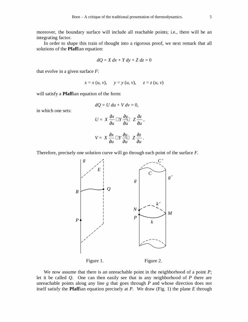
Therefore, precisely one solution curve will go through each point of the surface F.

P

R Q

E

g

P

N

g

C

C′

g′

k

M

k′

Figure 1. Figure 2.

We now assume that there is an unreachable point in the neighborhood of a point P; let it be called Q. One can then easily see that in any neighborhood of P there are unreachable points along any line g that goes through P and whose direction does not itself satisfy the Pfaffian equation precisely at P. We draw (Fig. 1) the plane E through


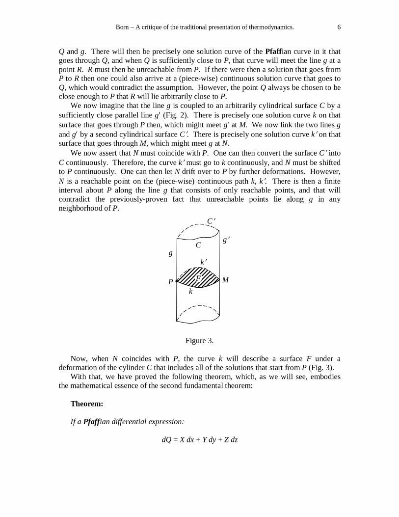
Q and g. There will then be precisely one solution curve of the Pfaffian curve in it that goes through Q, and when Q is sufficiently close to P, that curve will meet the line g at a point R. R must then be unreachable from P. If there were then a solution that goes from P to R then one could also arrive at a (piece-wise) continuous solution curve that goes to Q, which would contradict the assumption. However, the point Q always be chosen to be close enough to P that R will lie arbitrarily close to P. We now imagine that the line g is coupled to an arbitrarily cylindrical surface C by a sufficiently close parallel line g′ (Fig. 2). There is precisely one solution curve k on that surface that goes through P then, which might meet g′ at M. We now link the two lines g and g′ by a second cylindrical surface C′. There is precisely one solution curve k′ on that surface that goes through M, which might meet g at N. We now assert that N must coincide with P. One can then convert the surface C′ into C continuously. Therefore, the curve k′ must go to k continuously, and N must be shifted to P continuously. One can then let N drift over to P by further deformations. However, N is a reachable point on the (piece-wise) continuous path k, k′. There is then a finite interval about P along the line g that consists of only reachable points, and that will contradict the previously-proven fact that unreachable points lie along g in any neighborhood of P.

P

g C

C′

g′

k

M

k′

F

Figure 3.

Now, when N coincides with P, the curve k will describe a surface F under a deformation of the cylinder C that includes all of the solutions that start from P (Fig. 3). With that, we have proved the following theorem, which, as we will see, embodies the mathematical essence of the second fundamental theorem: Theorem: If a Pfaffian differential expression:

dQ = X dx + Y dy + Z dz


has the property that there is a point in any neighborhood of a point P (x, y, z) that is not reachable by solutions of the equation dQ = 0 then it will have an integrating factor. We add that there are also an infinite number of integrating factors then that can be constructed from one of them by using formula (13). All of these arguments can be carried over to Pfaffian differential expressions with more than three variables with no further discussion.

§ 6. – The second fundamental law.

Up to now, our representation of thermodynamics does not differ essentially from the traditional one, except that we have tried to define more precise concepts. The actual difference first emerges when one presents the second fundamental law. Naturally, the starting point is exactly the same, namely, the fact of experience that certain processes are impossible. However, the two representations already merge into each other when one formulates that fact and even more so in the derivation of the second fundamental law from it. In order to ease the comparison, we shall preface it with a sketch of the usual theory that we shall formulate as concisely and rigorously as possible.

I. The traditional representation.

The empirical basis is usually expressed by the principles of Clausius and Thomson, which read: Clausius’s principle: There is no mechanism that allows heat to flow from a colder heat-source to a hotter one in such a way that neither mechanical work will be done nor further changes will come about for distributed bodies. Thomson’s principle: There is no mechanism that allows a heat source to remove heat and convert it into work without the distributed bodies undergoing further changes (viz., the impossibility of the perpetuum mobile of the second kind). Both principles are equivalent to each other. One now considers a Carnot cycle. Ordinarily, one restricts oneself to gases for which all processes can be interpreted as curves in the pV-plane in order to do that, but naturally, that will not suffice for the general derivation of the second fundamental law. Most likely, one can restrict oneself to systems with three independent variables, because a further increase in the variables would require no new analysis. The state-space will then be three-dimensional. States in it with the same temperature will lie on the surfaces ϑ = const.


Those isothermal surfaces will cut out a one-parameter family of isotherms on any other surface F. At the same time, those two-dimensional surfaces F will be covered by a one-parameter family of adiabats (i.e., solutions of Pfaffian differential equation dQ = 0). The curvilinear rectangle in the surface F that is constructed from two isotherms ϑ1 and ϑ2 represents a Carnot cycle. One can realize it approximately when one first brings the system into contact with a very large heat-source W1 with a temperature ϑ1 that is practically constant and then alters it adiabatically until its temperature is ϑ2 . One then brings it into contact with a second heat-source W2 whose temperature is ϑ2 , and finally lets it return to its initial state adiabatically. If A is the work done on the system during the entire cycle, Q1 is the heat that is absorbed by W1, and Q2 is the heat that is given off by W2 then from the first fundamental law, one will have:

A = Q2 – Q1 . If ϑ1 < ϑ2 then one refers to the quotients:

1

A

Q= 2 1

1

Q Q

Q

−= 2

1

Q

Q− 1 (16)

as the “efficiency” of the “machine” that is composed of the system and the heat sources. It then follows from the principles of Clausius or Thomson that the efficiency for given ϑ1 , ϑ2 is not only independent of the type of Carnot cycle for one and the same system, but also for different systems that have the same value of their efficiency and operate between the same heat sources. In order to show that, one considers a composite process by which one machine performs a Carnot cycle in one sense and another machine performs a Carnot cycle in a different sense, and one arranges that either the works done are equal A = A′ or that the total heats that are supplied to the cooler heat reservoir W1 are equal Q1 = 1Q′ . Now, if:

1

A

Q>

1

A

Q

′′

then it will follow from the fact that A = A′ that one has both Q1 − 1Q′ < 0 and Q2 − 2Q′ <

0; i.e., the colder reservoir would absorb heat and the warmer one would supply it. It would follow from Q1 = 1Q′ that A − A′ > 0 and Q2 − 2Q′ > 0 ; i.e., the system would do

work only at the expense of the heat content of W2 . However, if:

1

A

Q<

1

A

Q

′′

then a consideration of the inverse process would yield the same contradiction to the principles of Clausius and Thomson. As a result:


2 1

1

Q Q

Q

−= G (ϑ1 , ϑ2) (17)

must be a universal function of the two temperatures ϑ1, ϑ2 of the heat sources, independently of the type of system, the chosen surface F, and the two adiabats. Now, if one sets ϑ1 =ϑ2 , ϑ2 = ϑ + ∆ϑ and lets ∆ϑ converge to zero then, since one obviously has G (ϑ , ϑ) = 0, one will get:

dQ

Q= g (ϑ) dϑ ,

in which one has set:

g (ϑ) = 1 2

1 2

2

( , )G

ϑ ϑ ϑ

ϑ ϑϑ

= =

∂ ∂

,

to abbreviate; g (ϑ) is also a universal function of ϑ. It would then follow that the heat supplied on an isotherm of the system would be:

Q = ( )g d

eϑ ϑ∫Ψ , (18)

in which Ψ depends upon the defining segments of the two adiabats and can be different for each system. One now considers a simple fluid, in particular, whose state is determined by two variables. The Pfaffian differential equation of the heat would then have an integrating factor, dQ = λ dϕ, and one could choose the quantities ϑ and ϕ to be the independent variables. Now, Ψ can depend upon the parameters ϕ1 , ϕ2 of the two adiabats of the Carnot process. Now, if one sets ϕ1 = ϕ , ϕ2 = ϕ + ∆ϕ and lets ∆ϕ converge to zero then if one recalls that obviously one will have Ψ (ϕ, ϕ) = 0, one will get:

dQ = Φ (ϕ) dϕ ( )g d

eϑ ϑ∫ ,

in which one sets:

Φ (ϕ) = 1 2

1 2

2

( , )

ϕ ϕ ϕ

ϕ ϕϕ

= =

∂Ψ ∂

,

to abbreviate. One now introduces the absolute temperature:

T = C( )g d

eϑ ϑ∫ , (61)

in which the constant C is fixed when one prescribes the difference in absolute temperature between any two fixed points – say, one sets it equal to 100o. If one further defines the entropy:


S = 1

( )dC

ϕ ϕΦ∫ (20)

and then gets the usual formulation of the second fundamental law:

dQ = T dS. (21) However, that formula is initially true only for simple fluids with two variables. Its extension to arbitrary systems would require special analysis. It would once more suffice to consider the case of three variables, for which the existence of an integrating factor is not trivial. Initially, one can express the efficiency of an arbitrary system in terms of the absolute temperature. From (18) and (19), one will then have:

Q = 1

TC

Ψ ,

and since Ψ has the same values for both isotherms of the Carnot process, it will follow that:

2 1

1

Q Q

Q

−= 2 1

1

T T

T

−

or

1

1

Q

T= 2

2

Q

T.

One can write this by saying that the line integral over a Carnot cycle is zero:

C

dQ

T∫= 0.

However, the same thing will be true for any closed, continuous curve K. If one then lays a surface F through that curve then one can construct a net of isotherms and adiabats on F, and one will obviously have:

K

dQ

T∫= lim

C

dQ

T∑∫ ,

in which the summation corresponds to the individual Carnot processes of the net inside the curve K, and the limit means the transition to an infinitely-fine mesh for the net. As a result one will have:

K

dQ

T∫= 0

for any closed curve; i.e., when the integral:


S = dQ

T∫

is extended from one point to a second one along any path, it will be independent of that path, and therefore a state function. One can generally prove that the absolute temperature of any thermodynamic system is an integrating factor of the differential of heat in the same way.

(Conclusion to follow)

_________



By. M. Born


(Conclusion)

_____

II. The new representation.

The crux of Carathéodory’s theory is the knowledge that with the help of the previously-proven theorems on Pfaffian differential expressions, a much more general formulation of the experimental principle that certain processes are impossible will suffice for one to arrive at the second fundamental law in the simplest way with no new physical analysis. Ordinarily, one gives much weight to formulating the experimental principle in such a way that it will exhibit as many processes as possible that are impracticable. It should be in no way possible to move heat from a colder body to a hotter one or to convert heat into work completely without some sort of “compensation.” However, the experience that there are certain impracticable processes at all does suffice for one to derive the second fundamental law completely. It will then suffice to refer to such primitive phenomena as the fact that an adiabatically-closed system cannot give up its energy content completely in the form of work. That is based upon the fact that when one chooses the forms and positions of the walls at the beginning and end of the process identically, such a system can become hotter by that process, but never colder. At most, one can arrange that the temperature will remain constant by performing the process quasi-statically. There will then be adiabatically-unreachable neighboring states, and indeed obviously in an arbitrary neighborhood of the starting state. However, it is entirely irrelevant for the consequences of thermodynamics to know which of the neighboring states are unreachable; it is enough that such things exist. We therefore formulate the fact of experience that is based upon the second fundamental law as follows: Carathéodory’s principle: In an arbitrary neighborhood of each state there are states that are not reachable from the initial state by adiabatic processes. In particular, there are, above all, neighboring states that are reachable by quasi-static, adiabatic processes, and thus, along adiabats.


It now follows, with the help of our mathematical analysis, that the Pfaffian differential expression dQ – viz., the differential of heat – always has an integrating factor, and that will then imply the formulas of thermodynamics with ease, while the traditional theory first sets the vast machinery of its cyclic processes in motion at that point. The principle teaches us nothing new immediately for a fluid whose state is determined by two variables – say, V, ϑ . That is because a Pfaffian expression in two variables will always have an integrating factor. One must then go on to systems with at least two bodies in thermal equilibrium. Something analogous also happens in the usual theory when one lets two machines perform Carnot cycles between the same heat sources in the opposite senses. However, one does not need to take that detour. One simply considers two bodies in thermal contact whose heat differential are given by formula (8′) and represents a Pfaffian expression of three variables V1 , V2 , ϑ . The union of our mathematical theorem with Carathéodory’s principle will then give the result that one can set:

dQ = dQ1 + dQ2 = λ dϕ , (22) in which λ and ϕ are certain state functions. On the other hand, one also has:

dQ1 = λ1 dϕ1 , dQ2 = λ2 dϕ2 , (23) so

λ dϕ = λ1 dϕ1 + λ2 dϕ2 . (24) One can now choose ϕ1 , ϕ2 , and ϑ to be the independent variables, instead of V1 , V2 . λ and ϕ can then be regarded as functions of ϕ1 , ϕ2 , ϑ, and formula (24) will show, with no further discussion, that:

1

ϕϕ

∂∂

= 1λλ

, 2

ϕϕ

∂∂

= 2λλ

, ϕϑ

∂∂

= 0. (25)

Due to the third of these equations, ϕ does not depend upon ϑ, but only upon ϕ1 and ϕ2 . As a result, the quotients:

1λλ

, 2λλ

will also be independent of ϑ :

1λϑ λ∂

∂= 0, 2λ

ϑ λ∂

∂= 0

or

1

1

1 λλ ϑ

∂∂

= 2

2

1 λλ ϑ

∂∂

= 1 λλ ϑ

∂∂

.


Now, λ1 is a state quantity for the first body, and thus depends upon only ϕ1 and ϑ. Likewise, λ2 is a state quantity of the second body, so it depends upon only ϕ2 and ϑ. The first equality sign can be valid only when both quantities depend upon only ϑ. Hence, one will have:

1logλϑ

∂∂

= 2logλϑ

∂∂

= logλ

ϑ∂

∂ = g (ϑ), (26)

in which the function g (ϑ) is universal. It will then have the same value for the two arbitrary bodies, as well as for the system that is composed of them. A brief argument will then lead to the existence of a universal temperature function with entirely “normal” mathematics, from which the usual temperature scale can be deduced by a simple normalization of the integrating factor. We shall now drop the index and understand λ to mean the integrating factor of an arbitrary system; it will then follow that:

log λ = ( )g dϑ ϑ∫ + log Φ, (27)

in which log Φ denotes the integration constant, which will depend upon the other state variables of the system, and for a fluid they would be just ϕ. Moreover, one gets:

λ = ( )g d

eϑ ϑ∫Φ . (28)

For any thermodynamic system, the integrating factor then splits into two factors, one of which depends upon only temperature and the other of which depends upon the remaining state variables. One then introduces the absolute temperature:

T = ( )g d

C eϑ ϑ∫ , (29)

in which the constant C is established when one prescribes the absolute temperature difference between two fixed points; one sets it equal to, say, 100o. With that definition, the differential of heat will become:

dQ = λ dϕ = T dC

ϕΦ⋅ ⋅ . (30)

If one is now dealing with an individual fluid then Φ can depend upon only ϕ. One can then define a state quantity that depends upon only ϕ by the formula:

S = 1

( ) dC

ϕ ϕΦ∫ , (31)

which is likewise constant on the adiabats. One calls it the entropy; it is defined up to an additive constant.


One then obtains the formula for the second fundamental law:

dQ = T dS ; (32) i.e., with that normalization, the absolute temperature will be the integrating factor of the differential of heat. However, the same thing is also true for a system of two bodies that are in thermal contact (and for an arbitrary system, in general). From (24) and (30), one will then have:

Φ dϕ = Φ1 dϕ1 + Φ2 dϕ2 , (33) so

1

ϕϕ

∂Φ∂

= Φ1 , 2

ϕϕ

∂Φ∂

= Φ2 .

Here, Φ1 depends upon only ϕ1 , and Φ2 depends upon only ϕ2 . If one now differentiates the first equation with respect to ϕ1 and the second one with respect to ϕ2 then one will get:

2

2 1 1 2

ϕ ϕϕ ϕ ϕ ϕ

∂Φ ∂ ∂+ Φ∂ ∂ ∂ ∂

= 0,

2

1 2 1 2

ϕ ϕϕ ϕ ϕ ϕ

∂Φ ∂ ∂+ Φ∂ ∂ ∂ ∂

= 0.

It will then follow by subtraction that the functional determinant is:

1 2

( , )

( , )

ϕϕ ϕ

∂ Φ∂

= 1 2 2 1

ϕ ϕϕ ϕ ϕ ϕ

∂Φ ∂ ∂Φ ∂−∂ ∂ ∂ ∂

= 0.

Thus, Φ will be a function of ϕ. One can then define the entropy by (31) for the system and from (33), one will have:

dS = dS1 + dS2 = d (S1 + S2) . (34) With a suitable determination of the additive constant, one might then set:

S = S1 + S2 . (35) The entropy of a system is the sum of the entropies of the subsystems. It should be remarked here that for complex systems, for which the components of their masses can be permuted, the additivity of the entropy must be proved in particular, which is always possible in a completely analogous way. We shall not pursue the design of the formal systems in thermodynamics any further, since we are concerned with only the basic principles.


§ 7. – Irreversible changes of state.

We shall now examine the behavior of entropy for arbitrary processes that are not quasi-static, and indeed, we shall initially consider the system that we have treated up to now that consists of two bodies in thermal contact. It depends upon three variables, which we previously chose to be V1 , V2 , and ϑ . Now, we would like to employ the entropy S, as the third variables instead of ϑ. Let 0

1V , 02V , and S0 be the values of the variables in the initial state, and let V1 , V2, S

be their values in the final state. We assert that for all possible processes S, they will be either non-increasing or non-decreasing. Namely, one can arrive at the final state by taking the following two steps: 1. One changes the volumes quasi-statically from 0

1V , 02V to V1 , V2 . The entropy

remains constantly equal to S0 during that. 2. One varies the state at constant volumes V1 , V2 by doing work adiabatically (stirring, friction, etc.) until the entropy has been converted from S0 into S. Now, if S were sometimes larger than S0 and sometimes smaller for different processes then every state V1 , V2, S that is in a neighborhood of the initial state 0

1V , 02V ,

S0 would be adiabatically reachable. Indeed, one could freely vary the volumes then. However, that contradicts the fact of experience that lies at the foundations of the second fundamental law. Hence, one must always have either S ≥ S0 or S ≤ S0. If one starts from another initial state then one will see that the impossibility of an increase or decrease in entropy must always be true in the same sense due to continuity. However, the same thing is also true for two different systems, due to the additivity property of entropy. Whether the entropy can only increase or only decrease depends upon the constant C in formula (29) [(31), resp.]. Naturally, one chooses it in such a way that the absolute temperature is positive. A single experiment will then suffice to establish the sign of the change in entropy. Experience shows that entropy never decreases (say, for gases; cf., infra, § 8). It will then follow that if the entropy is not constant for any change of state then no adiabatic change could be found that would take the system from the final state back to the initial one. In that sense, one has the theorem: Any change of state for which the value of the entropy varies is irreversible. Furthermore, that implies that entropy will have a maximum in equilibrium, and one will easily get the remaining extremal theorems of thermodynamics from this. We shall not go into that, but we must say a few words about the assumptions under which the proof that was given above for the systems that were considered here, which consist of two (or more) bodies in thermal contact, can be adapted to more complicated systems. The main idea was obviously that the two volumes could be varied completely independently of each other and that, other than those volumes, only one other variable –


viz., entropy – was present. Now, the corresponding statement is true in full generality: Not only that conclusion, but also the entire structure of thermodynamics, has to assume that for a system of n independent variables, n – 1 of them have the character of geometric quantities whose values one can vary arbitrarily, whereas only one “thermal” variable (e.g., temperature, entropy) is present. However, that restriction is not only characteristic of the Carathéodory form of thermodynamics, but is also true for the traditional theory, except that it does not emerge as clearly there in the derivation of the fundamental laws as it does here. Yet, it is probably sufficiently well-known that if one actually wishes to calculate the entropy in a special case then one must be in such a position that one can “perform the process reversibly.” However, that means nothing else but the fact that one can vary all variables except for one (the temperature) arbitrarily. In order to do that, one appeals to semi-permeable walls and similar artifices.

§ 8. – Examples.

We have explained the abstract train of thought in an entirely non-pedagogical way and not by examples, and we did that on purpose. Above all, we have not considered ideal gases, which play such a dominant role in many presentations of thermodynamics. It is precisely my opinion that this predominance of ideal gases brings with it the disadvantage that the student can easily come to think that all of thermodynamics depends upon the existence of certain gaseous substances. Naturally, there are presentations that rise above that flaw, but it is not avoided in other ones. In the latter, the gas temperature ϑ = pV seems to be the foundation for absolute temperature, and if it is also shown along the way that the latter is independent of the existence of particular bodies and can be determined by thermo-caloric measurements of various types then the process will be logically unsatisfying. There is not the slightest basis a priori for one to introduce precisely ϑ = pV as the empirical temperature, and not, say, ϑ = (pV)2 or any other (monotone) function ϑ = f (p ⋅⋅⋅⋅ V). Here, we would like to adopt that more general Ansatz and derive the absolute temperature from it; however, we still need the (calorimetric) determination of the energy function U. As usual, in order to do that, we appeal to the (idealized) Joule-Thomson experiment, which says that for an adiabatic expansion of a gas without any expenditure of work (in the first approximation), no change in the product pV [or the gas temperature ϑ = f (p ⋅⋅⋅⋅ V)] will occur. It follows from this that U will depend upon only ϑ. We then set:

pV = F (ϑ), U = U (ϑ). We define the adiabatic equation from this:

dQ = dU + p dV = U (ϑ) dϑ + F (ϑ) dV

V = 0.

If one writes:

dQ = F (ϑ)( )

log( )

Ud d V

F

ϑ ϑϑ

′ +


and sets:

log Θ (ϑ) = ( )

( )

Ud

F

ϑ ϑϑ

′∫

then one will have: dQ = F (ϑ) d log Θ V = 0.

Hence, one set: λ = F (ϑ), ϕ = log Θ V.

However, from (13), there are infinitely-many integrating factors; e.g., if one sets:

ϕ* = eϕ = Θ V then one will get:

λ* = d

d

ϕλϕ ∗ = F (ϑ) e−ϕ =

( )F

V

ϑΘ

.

There is absolutely no basis for singling out the integrating factor λ = F (ϑ) = pV, as is usually done. That is justified only by the second fundamental law, moreover. One will always find that:

g (ϑ) = log ( )d F

d

ϑϑ

from formula (26), in which ϕ is regarded as constant in the differentiation, and then from (29):

T = C F (ϑ) = C p V. The agreement of absolute temperature with the ideal gas scale is then proved with that. For the entropy, the formula dQ = T dS will then imply that:

S = S0 +1

Clog Θ V.

That will go over to the known expression when one sets:

U = c T, C = 1

R.

One will then have:

log Θ = c

dTRT∫ =

c

Rlog T,

so pV = RT, S = S0 – c log T + R log V.

A second example for the determination of absolute temperature is blackbody radiation. The empirical foundations are:


1. The radiation pressure p is connected with the energy density u by the formula:

p = 3

u.

2. The energy density depends upon only the temperature:

u = u (ϑ). The same thing is also true of p. The total energy in the volume V is:

U = 3 Vp. The Pfaffian equation for adiabats reads:

dQ = dU + p dV = 4p dV + 3V dp = 0, and can be written:

dQ = pV ⋅⋅⋅⋅ d log V 4 p3 = 0. One can then set:

λ = pV, ϕ = log V 4 p3. If one expresses λ as a function of p (ϑ) and ϕ then one will get:

log λ = 1

log4 4

pϕ+ .

Thus, from (26) and (27), one will have:

g (ϑ) = 1/4log p

ϑ∂

∂, log Φ =

4

ϕ,

and from (29): T = C p1/4.

One ordinarily employs the notation:

a = 4

3

C

and then obtains the Stefan-Boltzmann law:

u = 3p = a T 4. Furthermore, from (23), the entropy will be:

S = 1

dC

ϕΦ∫ = / 41e d

CϕΦ

∫ = / 44e

CΦ = 1/44

V pC

= 34

4V T

C= 34

3

aV T ,


when the constant is determined in such a way that S = 0 for T = 0. The entropy density is then:

s = 34

3

aT .

§ 9. – Generalizations.

We have already emphasized several times that our entire train of thought can be adapted to complex systems whose homogeneous components or phases can exchange matter with no further discussion, except that it must be possible to change all variables but one arbitrarily. Therefore, sufficiently-many empirical conditions must be given at any phase boundary to replace the simple condition of thermal equilibrium (e.g., an equation of state). Furthermore, one can introduce semi-permeable walls through which one can achieve the free mobility of the necessary number of arbitrarily-varying parameters. Since the theorems on Pfaffian equations are true for arbitrarily many variables, and not just three, all of our conclusions can be adapted with no further discussion. Whereas it is advantageous to avoid the usual cyclic processes in the general theory, for the actual calculation of thermodynamic functions, it is often quite convenient to use cyclic processes. In particular, Nernst’s theorem can be best evaluated in such a way that one employs cyclic processes with one branch that evolves from the absolute zero point. As Carathéodory emphasized, one will first encounter greater difficulties in the thermodynamic foundation of the theory of radiation and the processes in moving bodies, because the state of the system cannot be described by a finite number of parameters in those cases. Indeed, up to now, those domains have always been treated with only the statistical methods of kinetic theory.

(Received 25 November 1920)

___________

Documents

A critique of the traditional presentation of thermodynamicsneo-classical-physics.info/.../3/6/34363841/born_-_thermodynamics.pdf · A critique of the traditional presentation of