A data analytics case study assessing factors affecting ...eprints.qut.edu.au/68449/1/IJBIDM080301_NAYAK.pdf · methods such as Benkelman beam, ... A data analytics case study assessing

Int. J. Business Intelligence and Data Mining, Vol. 8, No. 3, 2013 199

Copyright © 2013 Inderscience Enterprises Ltd.

A data analytics case study assessing factors affecting pavement deflection values

Majid Seyfi, Rakesh Rawat, Justin Weligamage and Richi Nayak* Science and Engineering Faculty, Queensland University of Technology, Brisbane, Queensland, CBD QLD 4001, Australia and Department of Transport and Main Roads, P.O. Box 673, Fortitude Valley, Queensland, QLD 4006, Australia E-mail: [email protected] E-mail: [email protected] E-mail: [email protected] E-mail: [email protected] *Corresponding author

Abstract: Road networks are a national critical infrastructure. The road assets need to be monitored and maintained efficiently as their conditions deteriorate over time. The condition of one of such assets, road pavement, plays a major role in the road network maintenance programmes. Pavement conditions depend upon many factors such as pavement types, traffic and environmental conditions. This paper presents a data analytics case study for assessing the factors affecting the pavement deflection values measured by the traffic speed deflectometer (TSD) device. The analytics process includes acquisition and integration of data from multiple sources, data pre-processing, mining useful information from them and utilising data mining outputs for knowledge deployment. Data mining techniques are able to show how TSD outputs vary in different roads, traffic and environmental conditions. The generated data mining models map the TSD outputs to some classes and define correction factors for each class.

Keywords: data mining; classification; road pavement deflection.

Reference to this paper should be made as follows: Seyfi, M., Rawat, R., Weligamage, J. and Nayak, R. (2013) ‘A data analytics case study assessing factors affecting pavement deflection values’, Int. J. Business Intelligence and Data Mining, Vol. 8, No. 3, pp.199–226.

Biographical notes: Majid Seyfi is a PhD student at Queensland University of Technology. His research interests include data mining, database systems and software architecture. He received his MS in Computer Science from Arak Azad University of Iran.

Rakesh Rawat holds a PhD in Computer Science and his research area is related to data mining.

Justin Weligamage works at Queensland Transport and Main Roads and has several years of experience on road asset management.

200 M. Seyfi et al.

Richi Nayak is an Associate Professor in the Queensland University of Technology and has made significant contributions in applied data mining, semi-structured document mining, web personalisation, and social network mining. She has published over 120 refereed papers. She is an editorial board member of three journals. She serves as a program committee member to several conferences in the relevant area.

1 Introduction

A road network is considered as a critical national infrastructure which is always under high attention for its reliability. Considering safety and cost effectiveness as the primary goals, road asset management programmes include activities such as planning, maintenance and operation of road assets (Weligamage, 2002; Nayak et al., 2012). A report shows that 60% of investments in the road management programmes are allocated to the road pavement (Weligamage, 2002). The road pavement includes sub-base, base and wearing surface, and refers to the part of the road directly above the surface (Nayak et al., 2012). For effective road asset maintenance, it is necessary to have sufficient knowledge of the current situation of road pavements (Piyatrapoomi et al., 2001). The goal of every action in road maintenance is to keep the pavement condition in its highest utility with continued road access and lowest traffic inconvenience as well as reasonable cost (Abdulkareem, 2003; Rijn, 2006). Operational measurements of pavement conditions are needed to guide road agencies to set their priorities in the road maintenance programmes (Jenelius et al., 2006).

The traffic speed deflectometer (TSD), the world leading deflection testing technology developed recently in Denmark, is the latest technology of pavement deflection data collection up to the traffic speed of 80 kph. It can generate over 36 million data points per hour in its highest speed (Jenkins, 2009; Krarup et al., 2006). TSD has a high daily kilometric capability and high data resolution compared with earlier stationary methods such as Benkelman beam, deflectograph and falling weight deflectometer (FWD) (Jenkins, 2009; Krarup et al., 2006). Until now, TSD has mostly been used in European countries. Considering the cost-effectiveness and capacity of detailed examination of pavement structure, TSD has been trialled first time in Queensland in 2010 by the Queensland Department of Transport and Main Roads for measuring the pavement deflection of some selected roads in the network. Currently used technique for pavement condition monitoring is FWD. The TSD accuracy, however, is affected by many factors such as equipment operating conditions, environmental conditions, and road pavement conditions (Krarup et al., 2006). Moreover, due to the large amount of data collected by TSD, finding the inter-relationships between affecting factors of pavement deflection becomes a complex process.

Data mining has been driven by the need to solve practical problems (Nayak et al., 2006). Data mining is the process of finding distinct patterns and relationships that are hidden in large amounts of datasets (Fayyad et al., 1996). Data mining allows in assessing the significance of large number of variables in one single model (Nayak et al., 2012). In this paper we used this capability to model the higher resolution data received from the pavement condition monitoring machines with various traffic, environment and road conditions. Data analytics has been successfully applied in many areas such as

A data analytics case study assessing factors affecting pavement 201

marketing, medicine and finance (Fayyad et al., 1996; Melli et al., 2006; Nayak et al., 2006). Road transport and civil engineering are also areas where a variety of successful data mining applications are reported (Abugessaisa, 2008; Ge et al., 2008; Nayak et al., 2009, 2012).

In this paper, we present a case study for intelligently integrating information from several sources with the use of data mining and inform decision makers how the pavement conditions vary in different roads, traffic and environmental conditions. Data mining models have been generated to find inter-relationships of complex factors affecting pavement strength, especially the readings measured by TSD. This paper utilises data collected from the TSD trial that was carried out covering around 6,000 km of roads in the Queensland state controlled road network in May 2010. The other sources of data include

1 FWD data recording pavement deflection

2 assets data including pavement roughness, rutting, cracking and texture surface extracted from the organisation databases

3 traffic conditions, TSD and FWD equipments operating conditions

4 environmental conditions collected from Australian Bureau of Meteorology.

These datasets are divided in two groups:

1 the data monitored on seven trial roads

2 the data monitored on the wide network.

The goal of this paper is to assess the reliability of the TSD technology for Queensland conditions by comparing the TSD pavement deflection data with the historical FWD data in the road network. We have utilised methods such as decision tree and regression tree for determining the inter-relationships of complex factors. We present the extensive pre-processing method that included the generation of target classes by labelling the data based on different behaviours of TSD and FWD outputs. We also present some of the lessons that we learned by adopting a four phase data analytics methodology consisting of data pre-processing, data mining, result analysis and knowledge deployment. To our knowledge, this is a first study conducted for a government road agency.

The rest of the paper organised as follow. In the next section we show the similar real world applications and works related to road pavement assessment. In next sections, we present our work in four phases of the data mining process and then discuss the lessons learnt during the process. Finally we conclude the paper showing the future works.

2 Related work

This section covers two areas of related works. The first one is general applications of data mining in road safety. The second part covers the related work more specifically to pavement conditions.

Several researchers have used data mining techniques like classification and regression trees in real world applications for finding the inter-relationships between different domain attributes and predicting the variable behaviours (Wei and Keogh, 2006;

202 M. Seyfi et al.

Apte and Weiss, 1997; Anderson, 2009; Montella, 2011; Hojatia et al., 2013; Chang and Chen, 2005; Kashani and Mohaymany, 2011; Montella et al., 2011; Nayak et al., 2010; Emerson et al., 2011b, 2011b; Nayak et al., 2011). The reason behind their common usage is their prediction capability without setting any hypothesis or pre-defining underlying relationship between target variable and predictors (Chang and Chen, 2005). These techniques therefore have been utilised in road safety too.

Nayak et al. (2010, 2011) and Emerson et al. (2011b) proposed sophisticated data mining models to be used in the Queensland state main road network for identifying the relationships among crash, traffic and road variables in order to show the various road properties contributed in crashes. A case study is presented in Emerson et al. (2011b) for understanding the road crashes from relationships between skid resistance and other road attributes using predictive regression trees. Decision tree techniques are used for modelling the crash proneness of road segments using road and crash attributes (Nayak et al., 2011). In Emerson et al. (2011a) road network dataset was partitioned in group of classes based on their common characteristics using clustering methods.

Anderson (2009) defined the hotspots areas in road crashes of London, UK using the injury patterns of road crashes extracted from geographical information systems (GIS), kernel density estimation in road networks and clustering methods on environmental data. Effective prevention strategies are then developed for these high density areas to reduce the crash rate. Data mining techniques are used in Chang and Chen (2005) to show the relationships between traffic crashes and highway geometric variables, traffic characteristics, and environmental factors in the accident datasets from 2001–2002 of national freeway in Taiwan.

The classification and regression trees were used in Kashani and Mohaymany (2011) to define the factors influencing crash injury in rural roads in Iran over a 3-year period (2006–2008). In Hojatia et al. (2013) the classification techniques were proposed for mining the influence of different associated factors on accidents in the Australian freeway network. The association rule mining techniques are applied in Montella (2011) to define the interdependencies between large amount of affecting factors in crashes and the different crash types. In order to detect interdependence as well as dissimilarities among crash patterns, the data mining techniques, such as classification trees and association rules have been applied for the pedestrian data of 56,014 pedestrian crashes occurred in Italy in 2006–2008. Compare to probabilistic models in previous studies the results from this study were more consistent (Montella et al., 2011). Knowing the reasons behind existing deficiencies helped for better planning and designing of urban roads located in Italy.

Road agencies usually employ preventive and maintenance strategies and find ways to identify roads that need maintenance (Zhang et al., 2010). Road agencies are able to extend the pavements life cycle by slowing down the deterioration process by doing so. Research shows that the annual cost of maintenance for poor condition road pavements is more than four times in comparison to the cost of maintaining a good conditioned roads (Zhang et al., 2010).

In order to analyse the pavement life cycle, several research works have evaluated the relationships between road pavements structures and their environmental conditions. Some of the methods used for pavement infrastructure conditions evaluation are least-squares (parameter identification), database search, soft computing techniques such as neural networks, neuro-fuzzy systems, and genetic algorithms (Gopalakrishnan, 2010). There is an analytical study in finding relationship between the data measured by FWD in


trafficked and non-trafficked lanes using statistic methods to determine the degradation and rutting potential of flexible pavement unbound aggregate layers in comparison to the sub grade damages (Donovan and Tutumluer, 2009). Researchers have also looked for the relationship between temperature variation on the rigid pavements (Wang et al., 2009; Huang, 1993).

This paper uses the readings made by two devices to determine the various factors affecting the reading by one device. Time-series methods have been commonly used to compare a pair of time-variant datasets. This dataset poses several challenges such as different granularity, scale etc. Previous researchers (Wang et al., 2009) have used a mix of partitional and statistical approaches to compare two time-varying natures of the datasets. The datasets have been partitioned into several sections and the summaries of each section are derived using statistical comparisons. The change in statistical summaries reveals which datasets have changed and where. In the same line, this paper matches and compares two readings at the same locations, and their statistical variation is then used for building data mining models so that various sources of information can be integrated. To the best of our knowledge, this research is the first one in its kind that evaluates the pavement physical conditions using data mining to find about different factors that cause changes in deflection data measured by laser Dopplers in the TSD machine.

3 The data mining methodology

As we mentioned earlier, the primary goal of this case study is to compare the deflection values measured by TSD to the ones measured by FWD, which is widely and reliably used until now in Queensland road network. This comparison would lead us to determine the reliability model of the TSD in Australian conditions. The developed models should be able to establish correlations between the TSD and FWD data for the trial road network. It would clarify the road and environmental conditions for which the non-correlations exist and how they can be reformulated so that the correct TSD recordings can be considered. This is important to make sure that readings made by the two machines are done similarly or nearly similar in same road site locations.

Currently used FWD device operates at slow speed (5 km/hr) and results in high cost and traffic inconveniences. The FWD deflection values are measured at discrete points by dropping a weight on the road surface causing the pavement to deflect. It is built on a small trailer which remains stationary during a test (Weligamage et al., 2011). Compare to the direct measurement method of FWD, in TSD the pavement deflection is measured using highly advanced Doppler laser technology to provide continuous stream of deflection values and structural conditions of the roads without causing delay in traffic speed (80 km/hr) with generating 36 million data points per hour (Weligamage et al., 2011).

The TSD data processing, for generating the deflection values from the laser recordings, has been developed based on the road and environmental conditions in Europe which are very different from Australian conditions. Initial analysis shows that repetitive measurements in different environmental conditions can cause some variations in the reported results in the same road locations (Weligamage et al., 2011). Previous research has shown that the number of factors that affect TSD readings is not small and

204 M. Seyfi et al.

they are extracted from different categories of databases with different behaviours and complex interrelationships between them. For determining the affecting factors on TSD accuracy and the way they affect, we need to analyse all the different combinations of the candidate factors with TSD accuracy as a target attribute.

These characteristics of this case study make the data mining techniques a suitable candidate for solving this problem. We employ a four phase data mining methodology including

1 data and problem understanding

2 data preparation

3 data modelling

4 model interpretation and knowledge deployment.

The following sections describe each of the steps taken in the case study.

4 Data and problem understanding

This phase involves understanding the case study problem and acquisition of the related datasets. In order to analyse the road pavement deflection data, we use several distinct conditions of the pavement to be intelligently integrated into the developed data mining models. The pavement condition dataset used in this research can be categorised in three major groups:

• Structural strength and flexibility (deflection): The ability of a pavement to support traffic loading. This is used by agencies for the evaluation of material properties and structural capacity of pavements.

• Surface distress: The extent of pavement fracture, distortion and disintegration. It is measured in the form of cracking, rutting and longitudinal profile. This is used for the evaluation of deterioration and the maintenance needs of pavements.

• Roughness: The extent of irregularities found in the surface of pavements that affect the ride of a vehicle. This is used for the evaluation of the serviceability of pavements.

These three sets of conditions integrated with environmental and traffic conditions as well as pavement deflection measurements recorded by TSD and FWD devices are used to find the influencing factors affecting the TSD equipment accuracy. Road condition variables, based on their different characteristics, are measured on the predefined intervals such as every 100 metres, 400 metres, 800 metres or 1 km. These measurements are periodically evaluated during the pavement life cycle. The five categories of data used in data mining process are shown in Table 1. In this case study we used datasets generated in TSD trial roads of 6,000 km in the Queensland state controlled road network in May 2010.

The TSD device using laser technology can measure and record the road pavement variables. The recorded values are processed using a mathematical model and, as a final result, the pavement deflection value for a location is calculated. In our datasets, these values are collected every 1 metre, 5 metre or 10 metre intervals of road segments.


Table 1 List of input data

Data categories Attributes

TSD equipment operation data Vehicle testing speeds or velocity; axle loads; inner wheel path locations

Pavement condition data Pavement ( type, age, depth); seal age; aggregate sizes/texture, roughness, rutting

Traffic condition data Traffic volume, traffic speed limit Environmental data Road surface temperature; rainfall or road surface

moisture; air temperature Falling weight deflectometer (FWD) Deflection values Traffic speed deflectometer (TSD) Deflection values

4.1 Trial roads and network level datasets

The details of the TSD data in seven trial roads is shown in Table 2 where Chainage refers to the distance on road where trials were run, AADT refers to average annual daily traffic, type of pavement refers to the construction quality of the pavement, and WNR, DNR and DR are zone classifications. For seven trial roads, we obtained the corresponding environmental conditions as well as the pavement and traffic conditions from the organisation’s databases. Table 2 TSD and FWD datasets in seven trial roads

Site Road name Chainage Traffic (AADT)

Types of pavement Zone

10A Bruce highway 7.2–8.2 km 46,000 Deep asphalt WNR 10L Bruce highway 68–69 km 5,800 Granular WNR 10N Bruce highway 122–125 km 4,300 Granular WNR 14B Flinders highway 200–201 km 500 Granular DNR 13E Lands-borough highway 49–50 km 560 Granular DR 18D Warrego highway 93–94 km 1,250 Granular DNR 28A Gore highway 58.5–59.5 km 2,250 Granular DR

Same process was repeated for the dataset representing the wider network level. Because of the high measuring cost involved with FWD, its recordings are at an average of 500 metres intervals for the wider network whereas the FWD recordings are at 10 and 50 metres intervals for the seven trial roads. The next step is to understand the datasets quality and how the dataset was prepared for mining such as noise removal, normalisation and datasets integration.

5 Data pre-processing

Data preparation includes the activities for extracting a high quality dataset from the raw datasets for using in data mining process. It starts with integrating data extracted from different sources and modifying them based on the standard formats.

206 M. Seyfi et al.

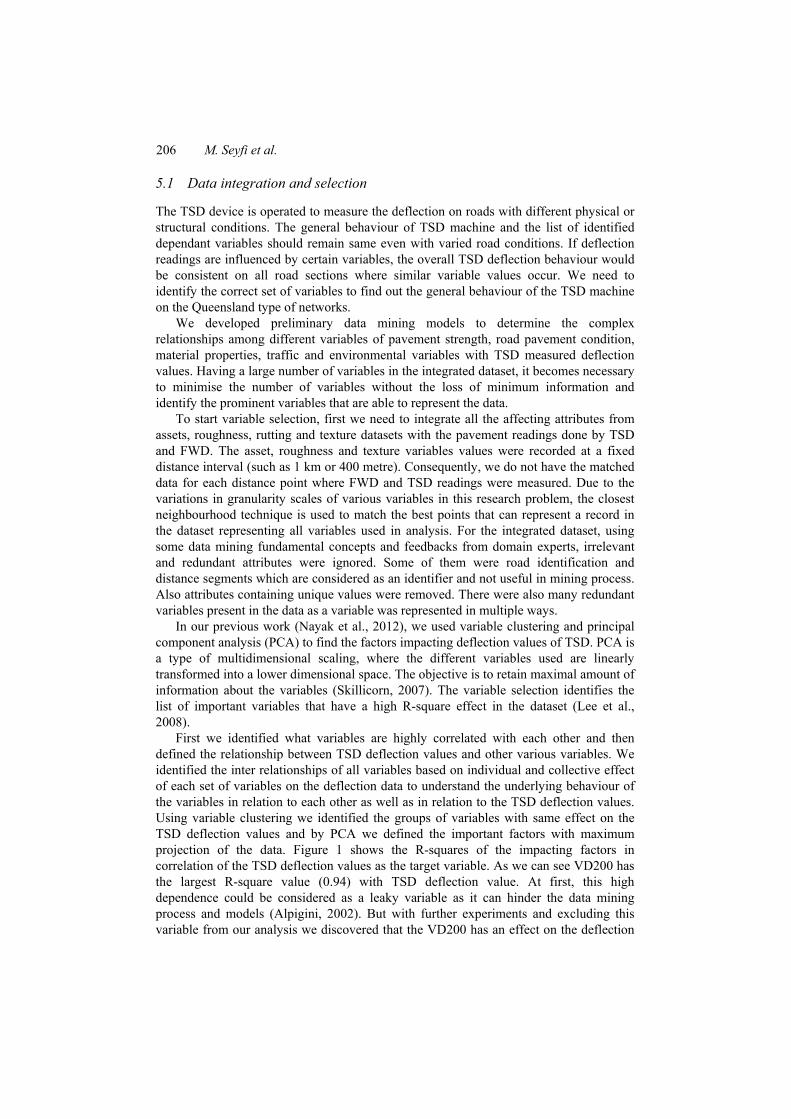
5.1 Data integration and selection

The TSD device is operated to measure the deflection on roads with different physical or structural conditions. The general behaviour of TSD machine and the list of identified dependant variables should remain same even with varied road conditions. If deflection readings are influenced by certain variables, the overall TSD deflection behaviour would be consistent on all road sections where similar variable values occur. We need to identify the correct set of variables to find out the general behaviour of the TSD machine on the Queensland type of networks.

We developed preliminary data mining models to determine the complex relationships among different variables of pavement strength, road pavement condition, material properties, traffic and environmental variables with TSD measured deflection values. Having a large number of variables in the integrated dataset, it becomes necessary to minimise the number of variables without the loss of minimum information and identify the prominent variables that are able to represent the data.

To start variable selection, first we need to integrate all the affecting attributes from assets, roughness, rutting and texture datasets with the pavement readings done by TSD and FWD. The asset, roughness and texture variables values were recorded at a fixed distance interval (such as 1 km or 400 metre). Consequently, we do not have the matched data for each distance point where FWD and TSD readings were measured. Due to the variations in granularity scales of various variables in this research problem, the closest neighbourhood technique is used to match the best points that can represent a record in the dataset representing all variables used in analysis. For the integrated dataset, using some data mining fundamental concepts and feedbacks from domain experts, irrelevant and redundant attributes were ignored. Some of them were road identification and distance segments which are considered as an identifier and not useful in mining process. Also attributes containing unique values were removed. There were also many redundant variables present in the data as a variable was represented in multiple ways.

In our previous work (Nayak et al., 2012), we used variable clustering and principal component analysis (PCA) to find the factors impacting deflection values of TSD. PCA is a type of multidimensional scaling, where the different variables used are linearly transformed into a lower dimensional space. The objective is to retain maximal amount of information about the variables (Skillicorn, 2007). The variable selection identifies the list of important variables that have a high R-square effect in the dataset (Lee et al., 2008).

First we identified what variables are highly correlated with each other and then defined the relationship between TSD deflection values and other various variables. We identified the inter relationships of all variables based on individual and collective effect of each set of variables on the deflection data to understand the underlying behaviour of the variables in relation to each other as well as in relation to the TSD deflection values. Using variable clustering we identified the groups of variables with same effect on the TSD deflection values and by PCA we defined the important factors with maximum projection of the data. Figure 1 shows the R-squares of the impacting factors in correlation of the TSD deflection values as the target variable. As we can see VD200 has the largest R-square value (0.94) with TSD deflection value. At first, this high dependence could be considered as a leaky variable as it can hinder the data mining process and models (Alpigini, 2002). But with further experiments and excluding this variable from our analysis we discovered that the VD200 has an effect on the deflection


values and it is independent in relation to any other variable. As the most influencing factor in the dataset, VD200 should be considered in analysis in any kind of modelling, when the dependant deflection variables is the target.

Figure 1 Effect of variables showed by R-square in relation to TSD deflection values (see online version for colours)

Table 3 Selected input variables for modelling process

Cluster name Variable

Seal_age

General_Terrain

Layer1Type

Pavement_Depth

AADT

Terrafic_Percentage_Heavy

Asset data

Formation_Type

Velocity

AirTemp

RoadTemp

TSD variables

VD200

Rutting data Rutting_80th_Percentile

International_Roughness_Index Roughness data

IRI_IWP (Roughness_Average)

Texture data SPTD_BWP_AVG

208 M. Seyfi et al.

Interestingly the results from PCA and variable clustering methods lead us to the almost same sort of variables with inter relationships to TSD defection value. From all these attributes we only chose the variables with higher impact on TSD deflection value and then identified the variables with similar behaviour in dataset, as the redundant attributes. After analysing the results from these two methods and also discussion with domain experts, a group of 15 attributes presented in Table 3 were selected as the input variables for data modelling (Nayak et al., 2012).

5.2 General pre-processing

We had a single variable measured by two different machines in dynamic distance scale. To compare this variable values that have been recorded in different measurement units and quantities, it was necessary to convert them to an equivalent scale in order to make a fair comparison. Scaling and normalisation of any dynamic data is essential as it is meaningless to compare two time series with different offsets and amplitudes (Wei and Keogh, 2006).

In FWD dataset, the deflection values have been measured with the combination of 40 kN, 60 kN and 80 kN weights, but for being comparable with the TSD dataset we needed to convert them to 50 kN. Based on the domain knowledge, multiplication of the deflection values from 40 kN measurement with a constant of 1.25 would give us the equivalent in 50 kN. A similar knowledge is used for converting the measurements done by 60 kN and 80 kN weights. Also, the direction of deflection values of both the devices is quite different. Whereas FWD has positive deflection values, TSD has negative deflection values. Based on our experiments (Nayak et al., 2012) by multiplication of the TSD deflection values with –1, the trend and magnitude of datasets do not get affected. The other challenging problem was that the FWD deflection values are in millimetre scale and TSD’s are in micron. We multiplied the FWD deflections by 1,000 to be in the same scale with TSD.

In the next step for having easier comparison, the deflection values from both machines are normalised in the range of 0 to 1. Based on the chart in Figure 6 (further down in the paper), in network level dataset, for FWD datasets we had very few numbers of points with deflection values upper than 2,500 (less than 2%) and for TSD in same intervals matched with FWD dataset, there were no deflection values higher than 1,500. In whole network dataset we have more than one million intervals measured by TSD. The chart presented in Figure 2 summarises the TSD deflection values in a way that each point shows the nominated maximum values for 10,000 of instances. In this chart, considering 4,000 as an outlier, as in more details it only refers to 0.03% values of the datasets, a value of 2,500 was chosen as the maximum deflection value in the TSD dataset. By simple division of each deflection value in these two machines by their maximum values we limited the range of deflection values in 0 to 1.

After doing these normalisation activities we applied point to point comparison to measure the differences in the TSD and FWD deflection values. Based on this comparison, in whole network datasets, the highest reported difference between deflection values from these two machines was 0.7 (Figure 5). We considered this as 100% difference rate and calculated the difference rate of other points based on that.


Figure 2 TSD maximum values in network datasets (see online version for colours)

5.3 Pre-processing in trial roads datasets

In TSD for some roads we have the measurements in combinations of 1 metre, 5 metre and 10 metre intervals and for some we only have them in 10 metre intervals. For better comparison, in seven different roads in the length of 1 kilometre each, the FWD measurements were applied in 10 and 50 metre intervals (Table 2). These datasets are integrated with TSD datasets using the point to point matching. In the roads 13E and 18D, all the collected datasets from two machines are with almost 5 metre differences. Because of these noises, in the modelling phase, we decided to not using data from these two roads. For the other five roads (10A, 10L, 10N, 14B and 28A) a total of 380 instances exist. To show that if the integrated datasets from FWD and TSD are in the exact same mileage, we added a new Boolean attribute called as ‘match’. The value of match is zero for a total of 152 instances, which means 40% of our collected datasets in two machines are not exactly at same points. However, as the differences were mostly less than 1 metre, these points were still good for modelling purpose.

Figure 3 compares the TSD and FWD data in trial site 10N in 50 metre intervals. In this chart, horizontal axis refers to the road distance intervals and vertical axis shows the normalised deflection values. In Figure 4, using difference rate, we can see the differences between TSD and FWD datasets in same trial site.

Figure 3 Deflection values in road section 10N – 50 m (see online version for colours)

210 M. Seyfi et al.

Figure 4 Difference rate in 10N – 50 m intervals (see online version for colours)

It can be seen from Figure 3 that the trends in FWD and TSD are usually same, and in majority of the times FWD values are higher than TSD values. This is visible too in Figure 4 by positive difference rates between their reported deflection values. By this comparison we can say that TSD reported lesser deflection values compared to FWD. These preliminary analyses also help us in highlighting some noise and errors in the datasets. For example in Figure 4, at the point 124,850, 3rd bar from the end, we have a very high spike in TSD value compared to FWD value. This indicates that it may happen because of GPS error which can be considered as a noise.

Table 4 shows the distribution of difference rate for five trial roads in six different categories. Based on this observation the best match for TSD and FWD data is in road section 10A and the worst matching is in road section 28A. The unique features of 10A in comparison to other trial roads (as shown in Table 2) are the Deep Asphalt type of pavement in 10A and the highest traffic range. It can also be ascertained that the road section 10A is in good condition as both machines gave low deflection values for this road (a lower deflection value depicts a better pavement condition). Based on discussion with domain experts, the likely reason for this good match would be the current good physical condition of 10A. Table 4 Distribution of difference rates in trial roads

Difference rate Road d ≤ –20 –20 < d

≤ –10 –10 < d ≤ 10

10 < d ≤ 25

25 < d ≤ 40 d >40

10A 61 (100%) 10L 43 (70%) 18 (30%) 10N 1 (1%) 81 (73%) 25 (23%) 3 (3%) 14B 3 (5%) 35 (61%) 19 (33%) 1 (1%) 28A 1 (1%) 17 (17%) 62 (62%) 18 (18%) 2 (2%)

The preliminary data analysis in these trial roads leads us to this conclusion that the TSD will record more accurate measurements in good condition roads. Of course the good roads are not in high consideration for road agencies. Also, the poor matching for the road section 28A may be due to the problems related to point to point comparison as in the most of the instances we have 1 metre differences in FWD and TSD intervals. This analysis warrants the need for creating data mining models to identify the affecting factors in TSD accuracy.


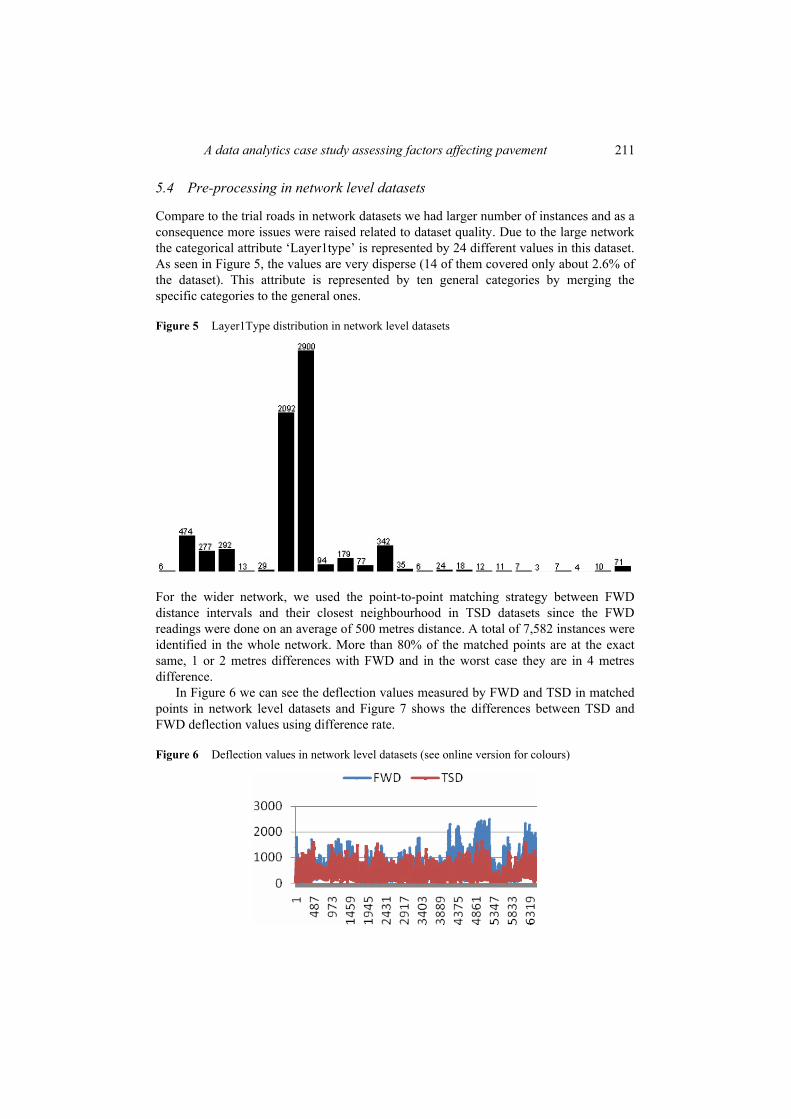
5.4 Pre-processing in network level datasets

Compare to the trial roads in network datasets we had larger number of instances and as a consequence more issues were raised related to dataset quality. Due to the large network the categorical attribute ‘Layer1type’ is represented by 24 different values in this dataset. As seen in Figure 5, the values are very disperse (14 of them covered only about 2.6% of the dataset). This attribute is represented by ten general categories by merging the specific categories to the general ones.

Figure 5 Layer1Type distribution in network level datasets

For the wider network, we used the point-to-point matching strategy between FWD distance intervals and their closest neighbourhood in TSD datasets since the FWD readings were done on an average of 500 metres distance. A total of 7,582 instances were identified in the whole network. More than 80% of the matched points are at the exact same, 1 or 2 metres differences with FWD and in the worst case they are in 4 metres difference.

In Figure 6 we can see the deflection values measured by FWD and TSD in matched points in network level datasets and Figure 7 shows the differences between TSD and FWD deflection values using difference rate.

Figure 6 Deflection values in network level datasets (see online version for colours)

212 M. Seyfi et al.

Figure 7 Difference rate in network level datasets (see online version for colours)

Same as trial roads, here we can see that FWD reported higher deflection values compare to TSD. In Table 5 the distribution of difference rate in network level datasets has been presented. Based on this table the error rate range in –10% to 10% is the most popular area. This can be described in this way that, in more than half of the times these two machines are doing same. Also we can see that the negative difference rates area is not very populated. Table 5 Distribution of difference rates in network level

Difference rate Road d ≤ –20 –20 < d

≤ –10 –10 < d ≤ 10

10 < d ≤ 25

25 < d ≤ 40 d >40

Number of instances 257 561 3529 1421 607 423 Percentage 3.7% 8.2% 52% 21% 9% 6.1%

Since the objective of mining process is to validate the accuracy of TSD machine on the Australian conditions, in the next step the difference rate is considered as a target value for creating the labelled classes. Several models have been built with varied labelling schemes.

6 Building data models

In order to analyse the factors affecting the TSD accuracy, we applied two different methods:

1 prediction using decision tree

2 prediction using regression tree.

These two methods have been applied in both the trial roads and network level datasets.


Decision tree and regression tree are popular predictive data mining techniques. They were chosen due to their capability of modelling the complex and non-linear relationships present in the dataset and producing high accuracy and comprehensible models so that the domain experts could understand the decision making process. We use the decision rules generated by models to predict the whole network reading measured by TSD. In decision tree we labelled our datasets based on different discrete categories of Difference_Rate, as a target value, and in regression tree we classify the instances based on numerical continues values of Difference_Rate.

6.1 Data modelling in trial roads datasets

In Figure 8 we can see the distribution of Difference_Rate across all the trial roads dataset. This figure reveals that the instances have been distributed in the range of –40% to 68% with disparity.

Figure 8 Distribution of Difference_Rate in trial roads

6.2 Decision tree

The large numbers of bins in Figure 7 is decomposed into five bins and a decision tree was generated with this class. The model achieved high accuracy (74%). This result was misleading as a total of 90% of instances were gathered in two classes due to the uneven class split. We explored further binning to accommodate different number of bins up to 15. However the outcomes were same.

As in trial roads the number of instances was small and also because of the heterogeneous distribution of Difference_Rate in a large range, we decided to try different labelling schemes by allocating each group of instances to the separated classes, based on their Difference_Rate as the target value, and then drive the classification rules for each class (Table 6).

In each scheme the instances within a specific Difference_Rate range were labeled in the same class label. With the classification schemes with large number of classes the confusion matrix was disperse in the truly classified instances. Based on this outcome, the further labeling schemes contain only the four classes. In the last two schemes as

214 M. Seyfi et al.

shown in Table 6, we had better accuracies but their confusion matrix reveals that most of the instances were classified in the two middle classes and the percentage of truly classified instances in the other classes was very low (zero to 20%). The kappa statistics and area under curve statistics were particularly used to show the imbalanced nature of the dataset and its effect on accuracy.

The forth scheme showed better classification in comparison with all other examined schemes. The confusion matrix of this scheme can be seen in Figure 9 and the decision rules extracted from the decision tree are presented in Figure 10. Table 6 Different labelled classes in trial roads

Six labelling schemes based on difference rate ranges Accuracy Number

of rules

Number of antecedence

nodes

Kappa statistics

Area under curve

1 ..–5 –5..5 5..15 15..25 25.. 59% 7 11 0.4284 0.8 2 ..–2 –2..8 8..18 18..28 28.. 54% 8 13 0.3338 0.793 3 ..–1 –1..9 9..19 19.. 60% 8 13 0.3956 0.816 4 ..–1 –1..10 10..20 20.. 61% 6 10 0.3893 0.805 5 ..–1 –1..10 10..25 25.. 64% 8 13 0.4309 0.801 6 ..–10 –10..10 10..20 20.. 65% 7 11 0.4044 0.814

Figure 9 Confusion matrix for scheme (...–1), (–1...10), (10...20), (20...)

Figure 10 Decision tree rules in trial roads

Seal_Age <= 3.6

| Velocity <= 21.68824

| | SPTD_BWP_AVG <= 2.14: 3 (75.0/39.0)

| | SPTD_BWP_AVG > 2.14: 2 (58.0/26.0)

| Velocity > 21.68824: 1 (47.0/30.0)

Seal_Age > 3.6

| DefMax <= –411.63695: 1 (54.0/6.0)

| DefMax > –411.63695

| | SPTD_BWP_AVG <= 2.32: 1 (113.0/21.0)

| | SPTD_BWP_AVG > 2.32: 2 (33.0/10.0)


6.3 Regression tree

As the target value ‘Difference_Rate’ is a continues variable, as an alternative approach, we tried to mine decision rules using regression tree techniques [M5 (Quinlan, 1992) and REPTree] and compared the extracted rules with the rules derived from decision trees. Using the M5 regression tree algorithm, we got a model with 59% accuracy and the following regression tree.

Figure 11 Regression tree from M5 algorithm in trial roads

Figure 12 Regression tree rules from M5 algorithm in trial roads

Layer1Type=31.0 <= 0.5: | Int_Roughness_Index <= 1.07: LM1 (76/16.023%) | Int_Roughness_Index > 1.07: LM2 (124/30.551%) Layer1Type=31.0 > 0.5: | SPTD_BWP_AVG <= 2.495: LM3 (125/100.336%) | SPTD_BWP_AVG > 2.495: | | DefMax <= –393.614: LM4 (21/82.35%) | | DefMax > –393.614: LM5 (34/91.128%)

As we can see the accuracy of this model is not very good. We tried more models with different settings to get a higher accuracy but as the number of instances in trial roads is very small for data mining process, we could not find better model with higher accuracy.

6.4 Data modelling in network level datasets

Out of the 7,000 instances remaining after outlier detection, more than 43% of matched points in FWD and TSD are in the same interval or have less than 1 metre differences. 35% of them are between 1 to 2 metre differences and in rest of the points we don’t have any differences more than 4 metre.

216 M. Seyfi et al.

6.4.1 Decision tree Based on the confusion matrix in different classification scheme and also looking at Table 7, same as trial roads dataset, we concluded that in this dataset we shouldn’t define more than four labelled classes. The first class is the main one as the most of the instances are in this populated area that covers the Difference_Rate around zero. The second class should cover the negative domain as if we define more than one label in this area then we won’t have any good percentage of truly classified instances in those classes. The other two classes should take care of positive domains. Compare to the negative domain, this area has wider range of values. However in the lower Difference_Rate we have more density. In Table 7 the information related to some of the different scheme have been presented.

Based on the first two schemes we found that in the classes with larger Difference_Rate the accuracy of classification is very low. This may be due to the reason that a good separation cannot be found in the difference rate in this domain based on the general characteristics of the road. In the third and fourth schemes we have relatively higher accuracy but their confusion matrices (Figure 13) reveal that most of the points classified in the middle class and for other two classes we don’t have good percentage of truly classified instances.

Figure 13 Confusion matrices for the third and fourth schemes in network level

Table 7 Different labelled classes in network level

Six labelling schemes based on difference rate ranges Accuracy Number

of rules

Number of antecedence

nodes

Kappa statistics

Area under curve

1 ..–15 –15..-5 –5..15 15..30 30.. 52% 53 132 0.1455 0.675

2 ..–10 –10..10 10..25 25..40 40.. 53% 46 74 0.153 0.689

3 ..–10 –10..20 20.. 69% 34 58 0.2369 0.704

4 ..–10 –10..25 25.. 74% 14 26 0.1558 0.678

5 ..–10 –10..10 10.. 62% 41 72 0.3185 0.721

6 ..–10 –10..10 10..20 20.. 57% 52 78 0.2517 0.696

The likely reason for less number of decision rules in these two could be because of these distributions as most of the instances classified in the middle class (83% in the third scheme and 90% in the fourth scheme). This can be seen in their kappa and area under curve statistics as well. The fifth scheme produces a good classifier with balanced classes. However having only one class for the Difference_Rates higher than 10% is not


enough, as because of large number of instances in this domain we need more than one category. We tried this with different scheme like scheme number 6, but almost in all of schemes we got very low percentage of truly classified instances in this area.

As an alternative way we adopted a two-step classification approach. First we defined the scheme (...–10), (–10...10), (10…) to classify our instances in three classes. The confusion matrix for this scheme can be seen in Figure 14.

Figure 14 Confusion matrix of fifth labelling scheme (Table 7)

We keep the decision rules representing from two classes (...–10) and –10...10). Instances representing the third class (the instances with Difference_Rate higher than 10%) are further split to define a new scheme. In this area we defined several schemes with two or more classes and we got the best result using two classes in the range of (10...23), (23...) with 70% accuracy. In total we report the scheme [(...–10) (–10...10) (10...23) (23...)] made in two steps with the total accuracy of 65%.

We had tried a model built with the classification scheme with four labelled classes (...–10), (–10...10), (10...23), (23...) in one step. However, as shown in confusion matrix (Figure 15) the third class is very bad in case of truly classified members. This shows that the two-step approach outperforms a single model built on these classes by distinctly representing the instances of the third class.

Figure 15 Confusion matrix for scheme (...–10), (–10...10), (10...23), (23...)

The rule analysis shows that the same set of attributes are involved in decision trees for the good classifications models and, most importantly, they appear in the same level in different decision trees. For example Defmax (deflection values measured by TSD) appears in root node in more than 95% of the models. This is followed by traffic volume and air temperature on the second level. The nominated scheme had the best similarity with most of the other good schemes and it has high accuracy and quality in its labelled classes. However as the size of trial roads datasets compare to network level dataset were so small, we found low similarities between decision rules in trial roads and network level datasets.

218 M. Seyfi et al.

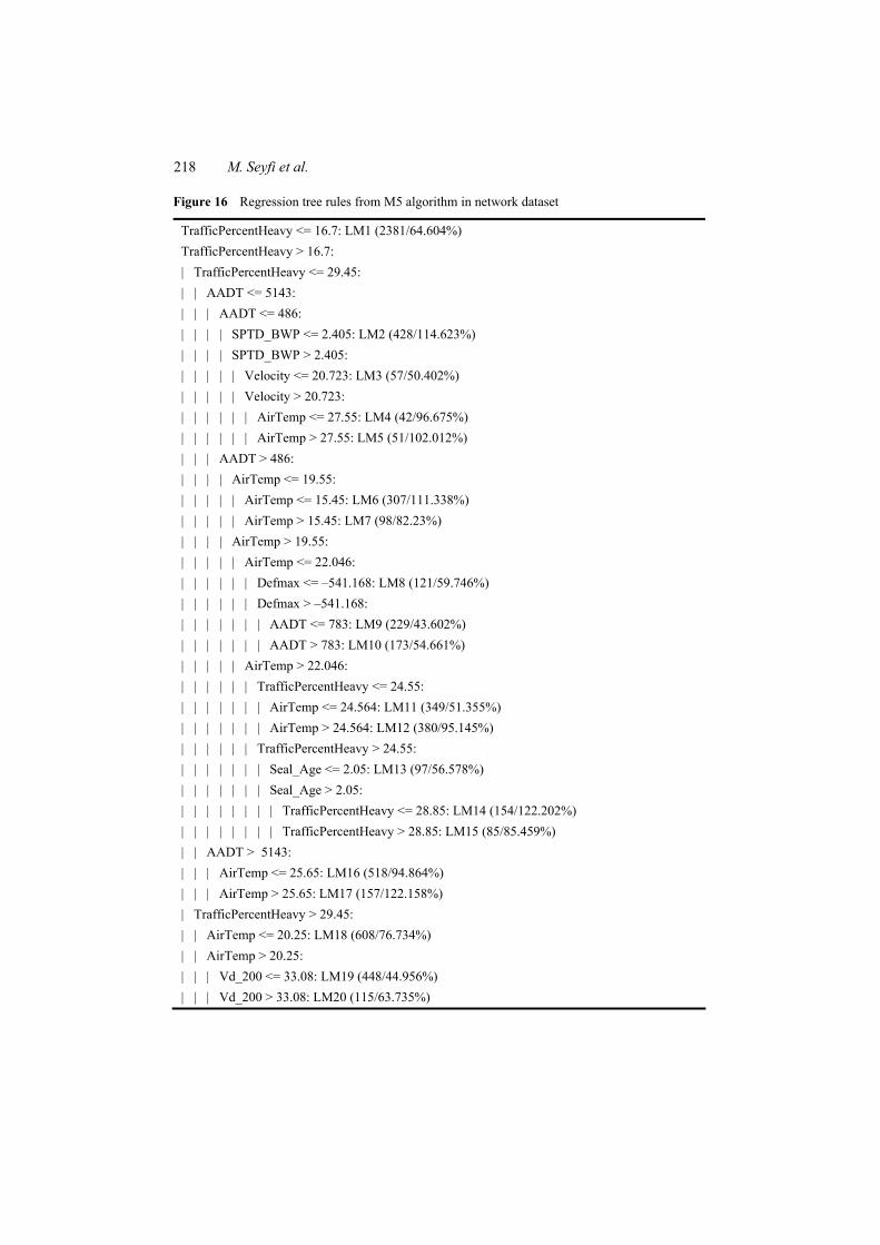
Figure 16 Regression tree rules from M5 algorithm in network dataset

TrafficPercentHeavy <= 16.7: LM1 (2381/64.604%) TrafficPercentHeavy > 16.7: | TrafficPercentHeavy <= 29.45: | | AADT <= 5143: | | | AADT <= 486: | | | | SPTD_BWP <= 2.405: LM2 (428/114.623%) | | | | SPTD_BWP > 2.405: | | | | | Velocity <= 20.723: LM3 (57/50.402%) | | | | | Velocity > 20.723: | | | | | | AirTemp <= 27.55: LM4 (42/96.675%) | | | | | | AirTemp > 27.55: LM5 (51/102.012%) | | | AADT > 486: | | | | AirTemp <= 19.55: | | | | | AirTemp <= 15.45: LM6 (307/111.338%) | | | | | AirTemp > 15.45: LM7 (98/82.23%) | | | | AirTemp > 19.55: | | | | | AirTemp <= 22.046: | | | | | | Defmax <= –541.168: LM8 (121/59.746%) | | | | | | Defmax > –541.168: | | | | | | | AADT <= 783: LM9 (229/43.602%) | | | | | | | AADT > 783: LM10 (173/54.661%) | | | | | AirTemp > 22.046: | | | | | | TrafficPercentHeavy <= 24.55: | | | | | | | AirTemp <= 24.564: LM11 (349/51.355%) | | | | | | | AirTemp > 24.564: LM12 (380/95.145%) | | | | | | TrafficPercentHeavy > 24.55: | | | | | | | Seal_Age <= 2.05: LM13 (97/56.578%) | | | | | | | Seal_Age > 2.05: | | | | | | | | TrafficPercentHeavy <= 28.85: LM14 (154/122.202%) | | | | | | | | TrafficPercentHeavy > 28.85: LM15 (85/85.459%) | | AADT > 5143: | | | AirTemp <= 25.65: LM16 (518/94.864%) | | | AirTemp > 25.65: LM17 (157/122.158%) | TrafficPercentHeavy > 29.45: | | AirTemp <= 20.25: LM18 (608/76.734%) | | AirTemp > 20.25: | | | Vd_200 <= 33.08: LM19 (448/44.956%) | | | Vd_200 > 33.08: LM20 (115/63.735%)


6.4.2 Regression tree Same as trial roads dataset, we applied regression tree methods [M5 (Quinlan, 1992) and REPTree] to see how different are their rules compare to the extracted rules from decision trees. By applying the regression tree algorithms using different settings we reached to a regression tree with reasonable size of tree and 20 decision rules with accuracy around 60%. We can see a good similarity between the derived rules from regression tree, (Figure 16) and the ones we mined from decision trees, especially in the attributes level in the decision rules.

6.5 Model interpretation and knowledge deployment

We tried different schemes for making labelled classes, both in trial roads datasets and network level datasets. The discovered rules from these two datasets are similar in many ways, even though, there are very low number of attributes and smaller range of data in trial roads. For example for ‘Layer1type’ we only have three different values but in network level after merging the disperse ones with the general categories we result in ten categorise which are always involved in our decision tree rules.

In network level dataset, looking at confusion matrix in Figure 14 we see a reasonable number of truly classified instances in class ‘b’ and class ‘c’. The class ‘a’ which covers the Difference_Rate less than –10% has not high number of truly classified members. This is true in any of the experimented schemes. Also we can see that the class ‘b’ is still the most populated range even in three labelled classes. The interesting characteristic of this confusion matrix and also confusion matrices from other schemes is that, false classified instances are mostly classified in their closed neighbourhoods. We used these distributions as one of our ways for boundary definition of the classes.

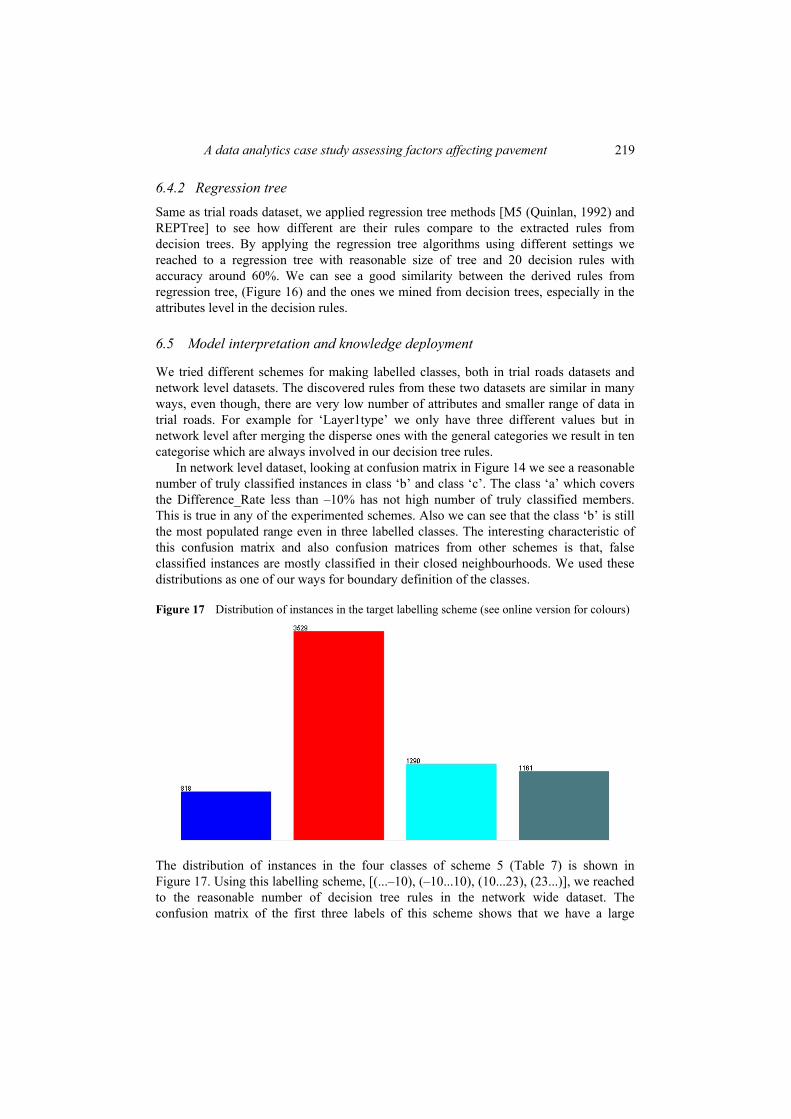
Figure 17 Distribution of instances in the target labelling scheme (see online version for colours)

The distribution of instances in the four classes of scheme 5 (Table 7) is shown in Figure 17. Using this labelling scheme, [(...–10), (–10...10), (10...23), (23...)], we reached to the reasonable number of decision tree rules in the network wide dataset. The confusion matrix of the first three labels of this scheme shows that we have a large

220 M. Seyfi et al.

number of truly classified instances (Figure 14). Also by comparing the kappa and area under curve statistics values of different schemes we can see better results in this scheme.

An interesting point in the process of defining different labeling scheme was that in most of these schemes, the generated decision rules were formed of same set of attributes and values. We tried several experiments with varied number of tree nodes, using minimum number of objects in each leaf. The results produced a marginal improvement (1% or 2% additional accuracy) but ended up generating larger trees with more rules. This resulted in more specific trees biased towards the training data.

Due to the noise present in the dataset and dependence of pavement deflection on many other factors than that of included in this model, the accuracy of mining models were limited to the ones obtained in this paper. Of course, for every small dataset we can have model with very high accuracy but it would be over fitting and not a general data mining model. These kinds of models only work well on that particular training datasets and are not applicable for other datasets.

As the decision tree is a classifier expressed as a recursive partition of the instance space, each path from the root to one of its leaves can be transformed into a rule simply by conjoining the tests along the path to form the antecedent part, and taking the leaf’s class prediction as the class value (Apte and Weiss, 1997).

The generated decision and regression trees are able to execute rules for each of the difference rate classes. An algorithm is used to map the extracted rules as the correction factors for the TSD readings under a particular road condition for each different rate category. Using these sets of rules any other set of measured deflection values by TSD integrated with selected variables, can be classified to one of the defined labelled classes and modified based on specified difference rates of those classes as its correction factor.

Based on the predictive features of decision tree, every new deflection values measured by TSD can be classified in one of these four classes. The predicted values can now be adjusted based on the boundary of the class it belongs to. For example, if an instance belongs to the class [10%..23%], considering the best case we add 10% of Difference_Rate to the real deflection value. In the worst case this would be 23% and in the average case 17%. However, the decision will be finalised by domain experts.

7 Lesson learned

In this section we show some of the significant lessons we learned during the data mining process.

7.1 Quality systems

The four phase data mining methodology (explore, modify, model and assess) proved invaluable in developing the data mining models and controlling their quality. The constant feedback and evaluation provided made a significant contribution to the maintenance of a quality process.


7.2 Importance of the database

The database proved to be an indispensable component of this project. Datasets were accessed from a number of sources and combined in a single integrated relational database. The database provided the following functionality and services to enable;

• data integrity to be maintained through the use of constraints

• procedures to be developed to support the initial pre-processing stage of combining the data

• procedures to be developed to obtain data views for developing datasets for the extensive data exploration

• data derived from post processing to be saved into the database for later use modelling and post processing.

7.3 Importance of data exploration

An extensive array of charts was produced to explore any data relationships that were described in other studies or by domain experts. The charts frequently confirmed that relationships existed, sometimes contradicted expert opinion and often posed questions. Charts or statistical operations were usually the reference point when a contentious result was obtained from data mining.

7.4 Meta data is critical

Context is crucial. When reading absorb the context, when writing outcomes provide the context. Context is lost when data is stored in databases, and that context must be rediscovered. It also reinforces the need to have meta-data information with data, models and results.

7.5 Garbage in – garbage out

Accuracy of data mining models and database integrity is of critical importance. If logic error in the data model or implementation error goes undetected the data mining will still produce misleading results. Having an effective feedback and evaluation mechanism is important as this is the best chance of detecting errors.

7.6 Good preparation

Preparation can be considered as the most important phase in data mining process. It is better to put enough time for this phase to avoid repetitive works in latter phases. Good data cleaning and preparation can speed up works in the next phases. Sometimes, making alternative description for original attributes or defining a new attribute based on combination of some primary attributes can give us better and more concise knowledge for the next phases.

222 M. Seyfi et al.

7.7 Always something missed

In real world applications we can never expect for perfect datasets. Datasets usually carry noises. Consequently, in some applications depending upon domain specific features, it is not expected to get very accurate result and approximation is acceptable.

7.8 Importance of good measures explaining the model generated

The correct selection of accuracy measures is critical to decide the model appropriateness for the problem. We observed that the classification accuracy measure was misleading to decide the model appropriateness for the problem. The contingency matrix further clarified which model was better. The use of kappa statistics and area under curve further confirmed the appropriateness of the models. Appropriate measures should be selected keeping in mind the dataset if it is imbalanced.

7.9 Domain knowledge

In real world applications it is critical to have close interaction with domain experts. Untimely poor interactions can lead to misunderstanding, wasting times and resources, and finally the useless results. Domain experts can be very helpful in data preparation phase as they know their datasets very well, however, in the technical phases analysts have to be more technological dependant.

7.10 Try and failure

Every data mining project is a mix of ‘try and failure’ iteration. It is very unlikely to get good results in the first iterations. Usually we fail in our ideas and solutions and then learn. The interesting point is that in every project we will face new issues.

7.11 Unbiased modelling

Data mining models have to be made unbiased. Almost for every project it is possible to have an over fitting models. General models, which can be fitted to every new datasets, would be with less accuracy but more reliability.

7.12 Knowledge production

Data mining is an automatic process that produces results. The human mind becomes the tool that evaluates the results and produces knowledge. Data mining results provide enhanced evidence. The human brain uses a cycle of observation, knowledge integration and knowledge analysis to draw conclusions. Inferences (possible explanations) are developed, further evidence is used to eliminate inferences and conclusions drawn. Generalisations are developed and tested.


7.13 Rooting data mining results in the real world

Data mining is an arcane and abstract activity. It may include:

1 operating in an environment a couple of steps away from reality

2 analysing data that has been affected by technical limitations

3 data in a biased subset

4 data that has errors

5 data that has had prior manipulation

6 data that could have had political interference

7 data that has been affected by security measures; and many others.

But still gems will be found. The importance of human intellect in interpreting the results cannot be overstated,

and developing connection with reality by knowing the domain and engaging domain experts is essential for the development of results and outcomes that will be trusted and applied to provide a business outcome.

7.14 Keeping the client happy

Where corporate databases are concerted, data mining is not a short term solution. We have been working on this study for over 18 months. At the start it is all slog, then at the end everything happens and keeps happening. The project needs to get over that threshold to survive. Clients require frequent feedback. Project milestones, early indicators and a succession of small wins help maintain the faith. These project management principles are important.

8 Conclusions and future works

This paper introduces a data analytics case study for assessing the effectiveness of a pavement deflection measuring technology. This paper highlighted the advancement of new data collection technology such as TSD that is able to provide better decision making for planning and budget procedures. This paper compared the readings done by TSD with FWD along with several traffic and road condition variables.

We presented the entire data mining process and highlighted the main findings. The application required integration of information from various sources. We propose to process the desperate sources of information intelligently with data mining models. We presented the data pre-processing steps necessary to prepare the datasets that required two devices to be compared. Several classifications schemes were generated to test the accuracy of the models built. The datasets used in modelling represent an uneven class distribution. Several specific measures such as kappa statistics and are under curve were used to deal with unbalanced dataset problem.

224 M. Seyfi et al.

This paper details various experiments that were conducted to identify the contributing factors that influence pavement deflection values. Using data mining process we showed that how the TSD deflection values will change under different environmental conditions, pavement types as well as other roads physical conditions. The dataset had noise present as well not every influencing factor was included in the dataset. Even though with these obstacles, we were able to build the data mining models with accuracies higher than 60%. The models were able to provide us insight into the dataset and explain the situations where the two machines do not highly correlate or do highly correlate.

This paper shows that with the advancement in computing resources and awareness of data analytics, the government road agencies are started to use automated methods of data analytics to understand their large amount of data that is stored in their organisation. Data analytics enable road managers to understand the complex relationships and dependencies amongst a large number of variables such as environmental, traffic, equipment operating and pavement conditions. The current means for identifying and budgeting for road maintenance rely heavily on the skill, experience and local road knowledge of people at the local level. Regional and state priorities are developed. Rehabilitation investment is based on manual inspection or previous year expenditure or assessment of pavement deterioration parameters such as roughness, rut depth, cracking, bad road sections and so on.

This paper presented an automated way to discover relationships that exist between various pavement condition variables that were not formerly known. Due to the complex and interrelated nature of pavement condition data collected from the TSD and many other sources, the task is beyond the scope of currently available methods available to engineers and managers, and their existing methods may not recognise many hidden and potentially useful relationships. Through data analytics complex pavement condition relationships were detected and knowledge was developed from datasets with large variable sets.

In our future work, using correction factors derived from decision trees and regression tress we plan to make a software program to get the TSD datasets in their raw formats and correct them based on the variation formula.

Acknowledgements

The study is part of the research project undertaken by Queensland University of Technology (QUT) and the Queensland Department of Transport and Main Roads (QDTMR), with sponsorship from the Cooperative Research Centre for Smart Services. The views presented in this paper are of the authors and not necessarily the views of the organisations.

References Abdulkareem, Y.A. (2003) ‘Road maintenance strategy, so far, how far?’, Nigerian Society of

Engineers Workshop on Sustainable Maintenance, Strategy of Engineering Infrastructures, llorin, Nigeria.

Abugessaisa, I. (2008) ‘Knowledge discovery in road accident database’, International Journal of Public Information Systems, Vol. 4, No. 1.


Alpigini, J.J. (2002) ‘Rough sets and current trends in computing’, The Proceedings of the Third International Conference, RSCTC 2002, Malvern, PA, USA, 14–16 October, Springer Verlag pp.24–75.

Anderson, T.K. (2009) ‘Kernel density estimation and K-means clustering to profile road accident hotspots’, Accident Analysis and Prevention, Vol. 41, No. 3, pp.359–364.

Apte, C. and Weiss, S. (1997) ‘Data mining with decision trees and decision rules’, Future Generation Computer Systems, November, Vol. 13, Nos. 2–3, pp.197–210.

Chang, L-Y. and Chen, W-C. (2005) ‘Data mining of tree-based models to analyze freeway accident frequency’, Journal of Safety Research, Vol. 36, No. 4, pp.365–375.

Donovan, P. and Tutumluer, E. (2009) ‘Falling weight deflectometer testing to determine relative damage in asphalt pavement unbound aggregate layers’, Transportation Research Record: Journal of the Transportation Research Board, Vol. 2104, No. 1, pp.12–23.

Emerson, D., Nayak, R. and Weligamage, J. (2011a) ‘Identifying differences in safe roads and crash prone roads using clustering data mining’, 6th World Congress on Engineering Asset Management (WCEAM 2011), Duke Energy Center, Cincinatti, Ohio.

Emerson, D., Nayak, R. and Weligamage, J. (2011b) ‘Using data mining to predict road crash count with a focus on skid resistance values’, 3rd International Road Surface Friction Conference Gold Coast, Queensland, Australia.

Fayyad, U.M., Piatetsky-Shapiro, G., Smyth, P. and Uthurusamy, R. (1996) ‘Advances in knowledge discovery and data mining’, in American Association for Artificial Intelligence, Menlo Park, CA.

Ge, E., Nayak, R., Xu, Y. and Li, Y. (Eds.) (2008) A User Driven Data Mining Process Model and Learning System, Springer, DASFAA.

Gopalakrishnan, K. (2010) ‘Instantaneous pavement condition evaluation using non-destructive neuro-evolutionary approach’, Structure and Infrastructure Engineering.

Hojatia, A.T., Ferreiraa, L., Washingtonb, S. and Charlesa, P. (2013) ‘Hazard based models for freeway traffic incident duration’, Accident Analysis and Prevention, No. 52, pp.171–181.

Huang, Y.H. (1993) Pavement Analysis and Design, 2nd ed., Pearson Education, Inc., Upper Saddle River, NJ.

Jenelius, E., Petersen, T. and Mattsson, L-G. (2006) ‘Importance and exposure in road network vulnerability analysis’, Transportation Research Part A: Policy and Practice, Vo. 40, No. 7, pp.537–560.

Jenkins, M. (2009) ‘Geometric and absolute calibration of the english highways agency traffic speed deflectometer’, in Young Researchers Seminar, Session, Road Transport, Italy.

Kashani, A.T. and Mohaymany, A.S. (2011) ‘Analysis of the traffic injury severity on two-lane, two-way rural roads based on classification tree models’, Safety Science, December, Vol. 49, No. 10, pp.1314–1320.

Krarup, J., Rasmussen, S., Aagaard, L. and Hjorth, P.G. (Eds.) (2006) ‘Output from the Greenwood traffic speed deflectometer’, 22nd ARRB Conference – Research into Practice, Canberra, Australia.

Lee, T., Duling, D., Liu, S. and Latour, D. (Eds.) (2008) ‘Two-stage variable clustering for large data sets’, SAS Global Forum, SAS Institute Inc.

Melli, G., Zaïane, O.R. and Kitts, B. (2006) ‘Introduction to the special issue on successful real-world data mining applications’, ACM SIGKDD Explorations Newsletter, Vol. 8, No. 1, pp.1–2.

Montella, A. (2011) ‘Identifying crash contributory factors at urban roundabouts and using association rules to explore their relationships to different crash types’, Accident Analysis and Prevention, July, Vol. 43, No. 4, pp.1451–1463.

Montella, A., Aria, M., D’Ambrosio, A. and Mauriello, F. (2011) ‘Data mining techniques for exploratory analysis of pedestrian crashes’, TRB Annual Meeting.

226 M. Seyfi et al.

Nayak, R., Buys, L. and Lovie-Kitchin, J. (Eds.) (2006) ‘Influencing factors in achieving active ageing. optimization -based data mining techniques with applications’, A Workshop of IEEE International Conference on Data Mining, IEEE, Hong Kong, December.

Nayak, R., Emerson, D., Weligamage, J. and Piyatrapoomi, N. (2010) ‘Using data mining on road asset management data in analysing road crashes’, 16th Annual TMR Engineering & Technology Forum, Brisbane, Australia.

Nayak, R., Emerson, D., Weligamage, J. and Piyatrapoomi, N. (2011) Road Crash Proneness Prediction Using Data Mining, EDBT, Uppsala, Sweden.

Nayak, R., Piyatrapoomi, N. and Weligamage, J. (Eds.) (2009) ‘Application of text mining in analysing road crashes for road asset management’, World Congress in Engineering Asset Management, World Congress on Engineering Asset Management, Greece.

Nayak, R., Rawat, R. and Weligamage, J. (2012) ‘A data analytics application assessing pavement deflection factors for a road network’, Proceedings of the 14th International Conference on Information Integration and Web-based Applications & Services (IIWAS '12), pp.247–255.

Piyatrapoomi, N., Kumar, A., Robertson, N. and Weligamage, J. (2001) Assessment of Calibration Factors for Road Deterioration Models, CRC CI Report No. -010-C/009, The Cooperative Research Centre for Construction Innovation, Queensland University of Technology, Brisbane, Queensland, Australia.

Quinlan, J.R. (1992) ‘Learning with continuous classes’, in the Proceedings of the Second Australian Conference on Artificial Intelligence, Singapore.

Rijn, J.V. (2006) Maintenance of Road Structures, Indevelopment. Skillicorn, D.B. (2007) Understanding Complex Datasets: Data Mining with Matrix

Decompositions, Chapman & Hall/CRC. Wang, D., Roesler, J.R. and Guo, D.Z. (2009) ‘Analytical approach to predicting temperature fields

in multilayered pavement systems’, Journal of Engineering Mechanics, pp.135–334. Wei, L. and Keogh, E. (2006) ‘Semi-supervised time series classification’, ACM SIGKDD,

pp.748–753. Weligamage, J. (2002) Asset Maintenance Guidelines, Road Asset Management Branch, Technical

Report in Queensland Department of Transport and Main Roads, Queensland, Australia. Weligamage, J., Piyatrapoomi, N. and Gunapala, L. (2011) Techniqal Report of Traffic Speed

Deflectometer, Queensland Trial. Zhang, Z., Jaipuria, S., Murphy, M.R., Sims, T. and Garza, T. (2010) ‘Pavement preservation.

transportation research record’, Journal of the Transportation Research Board, Vol. 2150, No. 1, pp.28–35.

Documents

A data analytics case study assessing factors affecting ...eprints.qut.edu.au/68449/1/IJBIDM080301_NAYAK.pdf · methods such as Benkelman beam, ... A data analytics case study assessing