Embed Size (px)
Citation preview
A Deep Q-Network for the Beer Game: AReinforcement Learning Algorithm to Solve
Inventory Optimization Problems
Afshin Oroojlooyjadid, MohammadReza Nazari, Lawrence V. Snyder, Martin TakacDepartment of Industrial and Systems Engineering, Lehigh University, Bethlehem, PA 18015,
{oroojlooy, mon314, larry.snyder, mat614}@lehigh.edu
The beer game is a widely used in-class game that is played in supply chain management classes to demon-
strate the bullwhip effect. The game is a decentralized, multi-agent, cooperative problem that can be modeled
as a serial supply chain network in which agents cooperatively attempt to minimize the total cost of the net-
work even though each agent can only observe its own local information. Each agent chooses order quantities
to replenish its stock. Under some conditions, a base-stock replenishment policy is known to be optimal.
However, in a decentralized supply chain in which some agents (stages) may act irrationally (as they do in
the beer game), there is no known optimal policy for an agent wishing to act optimally.
We propose a machine learning algorithm, based on deep Q-networks, to optimize the replenishment
decisions at a given stage. When playing alongside agents who follow a base-stock policy, our algorithm
obtains near-optimal order quantities. It performs much better than a base-stock policy when the other
agents use a more realistic model of human ordering behavior. Unlike most other algorithms in the literature,
our algorithm does not have any limits on the beer game parameter values. Like any deep learning algorithm,
training the algorithm can be computationally intensive, but this can be performed ahead of time; the
algorithm executes in real time when the game is played. Moreover, we propose a transfer learning approach
so that the training performed for one agent and one set of cost coefficients can be adapted quickly for other
agents and costs. Our algorithm can be extended to other decentralized multi-agent cooperative games with
partially observed information, which is a common type of situation in real-world supply chain problems.
Key words : Inventory Optimization, Reinforcement Learning, Beer Game
History :
1
arX
iv:1
708.
0592
4v2
[cs
.LG
] 8
Mar
201
8

Author: Article Short Title2
1. Introduction
The beer game consists of a serial supply chain network with four agents—a retailer, a warehouse,
a distributor, and a manufacturer—who must make independent replenishment decisions with
limited information. The game is widely used in classroom settings to demonstrate the bullwhip
effect, a phenomenon in which order variability increases as one moves upstream in the supply
chain. The bullwhip effect occurs for a number of reasons, some rational (Lee et al. 1997) and some
behavioral (Sterman 1989). It is an inadvertent outcome that emerges when the players try to
achieve the stated purpose of the game, which is to minimize costs. In this paper, we are interested
not in the bullwhip effect but in the stated purpose, i.e., the minimization of supply chain costs,
which underlies the decision making in every real-world supply chain. For general discussions of
the bullwhip effect, see, e.g., Lee et al. (2004), Geary et al. (2006), and Snyder and Shen (2018).
The agents in the beer game are arranged sequentially and numbered from 1 (retailer) to 4
(manufacturer), respectively. (See Figure 1.) The retailer node faces stochastic demand from its
customers, and the manufacturer node has an unlimited source of supply. There are determinis-
tic transportation lead times (ltr) imposed on the flow of product from upstream to downstream,
though the actual lead time is stochastic due to stockouts upstream; there are also deterministic
information lead times (lfi) on the flow of information from downstream to upstream (replenish-
ment orders). Each agent may have nonzero shortage and holding costs.
In each period of the game, each agent chooses an order quantity q to submit to its predecessor
(supplier) in an attempt to minimize the long-run system-wide costs,
T∑t=1
4∑i=1
cih(ILit)+ + cip(IL
it)−, (1)
where i is the index of the agents; t= 1, . . . , T is the index of the time periods; T is the (random)
time horizon of the game; cih and cip are the holding and shortage cost coefficients, respectively, of
agent i; and ILit is the inventory level of agent i in period t. If ILit > 0, then the agent has inventory
on-hand, and if ILit < 0, then it has backorders, i.e., unmet demands that are owed to customers.
The notation x+ and x− denotes max{0, x} and max{0,−x}, respectively.

Author: Article Short Title3
Figure 1 Generic view of the beer game network.
4Manufacturing
3Distributor
2Wholesaler
1Retailer
CustomerSupplier
The standard rules of the beer game dictate that the agents may not communicate in any way,
and that they do not share any local inventory statistics or cost information with other agents
until the end of the game, at which time all agents are made aware of the system-wide cost. In
other words, each agent makes decisions with only partial information about the environment while
also cooperating with other agents to minimize the total cost of the system. According to the
categorization by Claus and Boutilier (1998), the beer game is a decentralized, independent-learners
(ILs), multi-agent, cooperative problem.
The beer game assumes the agents incur holding and stockout costs but not fixed ordering costs,
and therefore the optimal inventory policy is a base-stock policy in which each stage orders a suffi-
cient quantity to bring its inventory position (on-hand plus on-order inventory minus backorders)
equal to a fixed number, called its base-stock level (Clark and Scarf 1960). When there are no
stockout costs at the non-retailer stages, i.e., cip = 0, i∈ {2,3,4}, the well known algorithm by Clark
and Scarf (1960) (or its subsequent reworkings by Chen and Zheng (1994), Gallego and Zipkin
(1999)) provides the optimal base-stock levels. To the best of our knowledge, there is no algorithm
to find the optimal base-stock levels for general stockout-cost structures, e.g., with non-zero stock-
out costs at non-retailer agents. More significantly, when some agents do not follow a base-stock
or other rational policy, the form and parameters of the optimal policy that a given agent should
follow are unknown. In this paper, we propose a new algorithm based on deep Q-networks (DQN)
to solve this problem.
The remainder of this paper is as follows. Section 2 provides a brief summary of the relevant
literature and our contributions to it. The details of the algorithm are introduced in Section 3.
Section 4 provides numerical experiments, and Section 5 concludes the paper.
Author: Article Short Title4
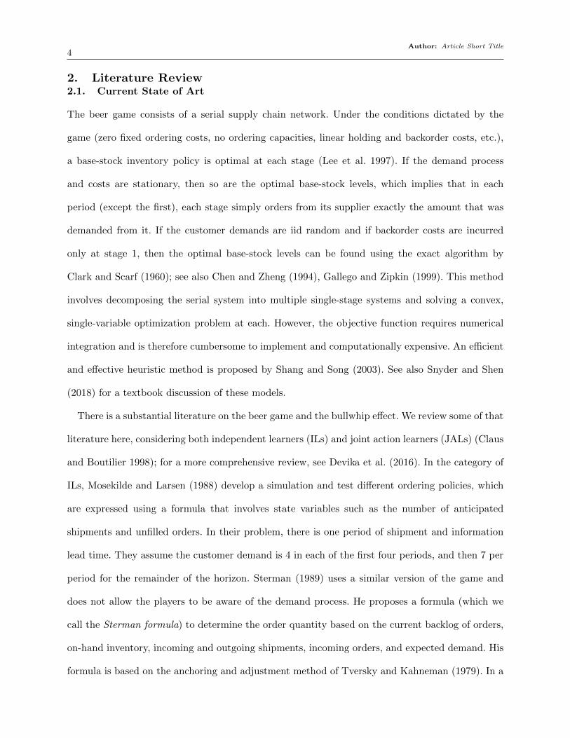
2. Literature Review2.1. Current State of Art
The beer game consists of a serial supply chain network. Under the conditions dictated by the
game (zero fixed ordering costs, no ordering capacities, linear holding and backorder costs, etc.),
a base-stock inventory policy is optimal at each stage (Lee et al. 1997). If the demand process
and costs are stationary, then so are the optimal base-stock levels, which implies that in each
period (except the first), each stage simply orders from its supplier exactly the amount that was
demanded from it. If the customer demands are iid random and if backorder costs are incurred
only at stage 1, then the optimal base-stock levels can be found using the exact algorithm by
Clark and Scarf (1960); see also Chen and Zheng (1994), Gallego and Zipkin (1999). This method
involves decomposing the serial system into multiple single-stage systems and solving a convex,
single-variable optimization problem at each. However, the objective function requires numerical
integration and is therefore cumbersome to implement and computationally expensive. An efficient
and effective heuristic method is proposed by Shang and Song (2003). See also Snyder and Shen
(2018) for a textbook discussion of these models.
There is a substantial literature on the beer game and the bullwhip effect. We review some of that
literature here, considering both independent learners (ILs) and joint action learners (JALs) (Claus
and Boutilier 1998); for a more comprehensive review, see Devika et al. (2016). In the category of
ILs, Mosekilde and Larsen (1988) develop a simulation and test different ordering policies, which
are expressed using a formula that involves state variables such as the number of anticipated
shipments and unfilled orders. In their problem, there is one period of shipment and information
lead time. They assume the customer demand is 4 in each of the first four periods, and then 7 per
period for the remainder of the horizon. Sterman (1989) uses a similar version of the game and
does not allow the players to be aware of the demand process. He proposes a formula (which we
call the Sterman formula) to determine the order quantity based on the current backlog of orders,
on-hand inventory, incoming and outgoing shipments, incoming orders, and expected demand. His
formula is based on the anchoring and adjustment method of Tversky and Kahneman (1979). In a
Author: Article Short Title5
nutshell, the Sterman formula attempts to model the way human players over- or under-react to
situations they observe in the supply chain such as shortages or excess inventory. There are multiple
extensions of Sterman’s work. For example, Strozzi et al. (2007) considers the beer game when the
customer demand increases constantly after four periods and proposes a genetic algorithm (GA)
to obtain the coefficients of the Sterman model. Subsequent behavioral beer game studies include
Kaminsky and Simchi-Levi (1998), Croson and Donohue (2003) and Croson and Donohue (2006).
Most of the optimization methods described in the first paragraph of this section assume that
every agent follows a base-stock policy. The hallmark of the beer game, however, is that players
do not tend to follow such a policy, or any policy. Often their behavior is quite irrational. There is
comparatively little literature on how a given agent should optimize its inventory decisions when the
other agents do not play rationally (Sterman 1989, Strozzi et al. 2007)—that is, how an individual
player can best play the beer game when her teammates may not be making optimal decisions.
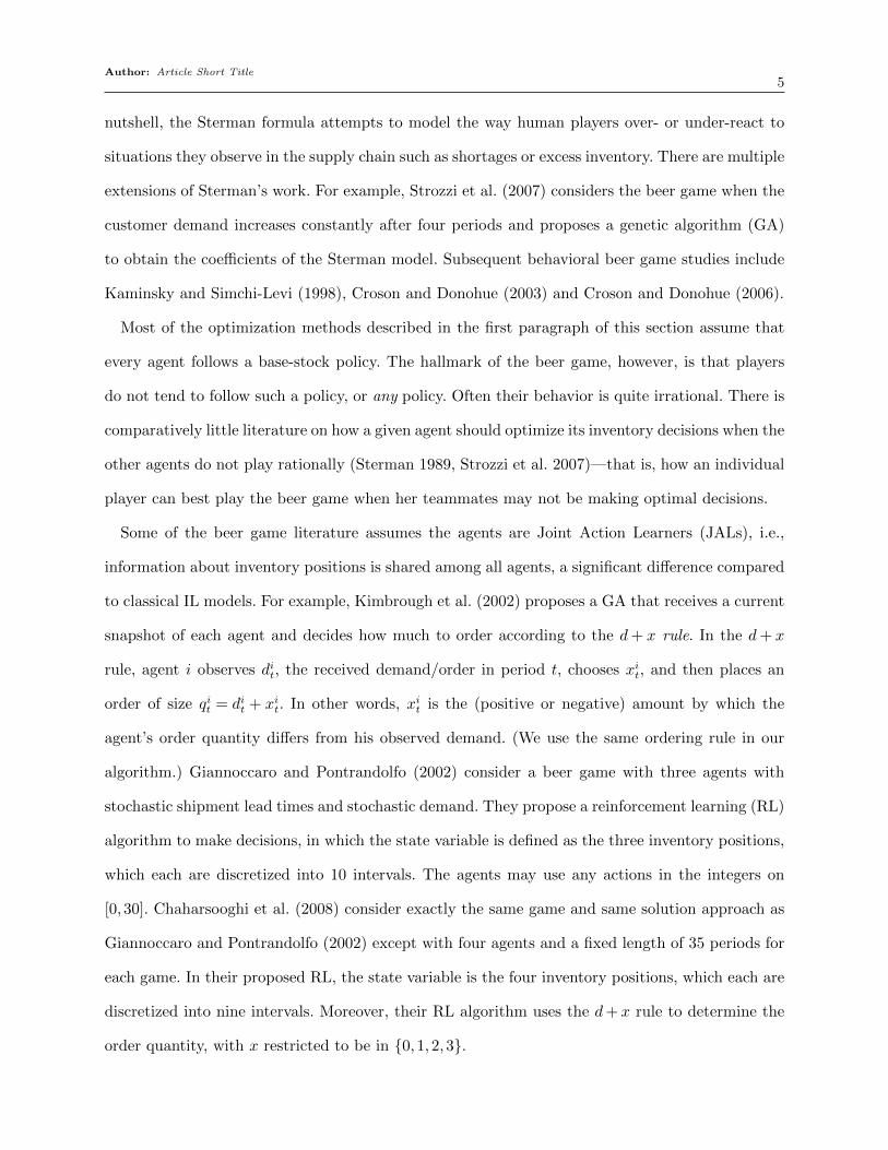
Some of the beer game literature assumes the agents are Joint Action Learners (JALs), i.e.,
information about inventory positions is shared among all agents, a significant difference compared
to classical IL models. For example, Kimbrough et al. (2002) proposes a GA that receives a current
snapshot of each agent and decides how much to order according to the d+ x rule. In the d+ x
rule, agent i observes dit, the received demand/order in period t, chooses xit, and then places an
order of size qit = dit + xit. In other words, xit is the (positive or negative) amount by which the
agent’s order quantity differs from his observed demand. (We use the same ordering rule in our
algorithm.) Giannoccaro and Pontrandolfo (2002) consider a beer game with three agents with
stochastic shipment lead times and stochastic demand. They propose a reinforcement learning (RL)
algorithm to make decisions, in which the state variable is defined as the three inventory positions,
which each are discretized into 10 intervals. The agents may use any actions in the integers on
[0,30]. Chaharsooghi et al. (2008) consider exactly the same game and same solution approach as
Giannoccaro and Pontrandolfo (2002) except with four agents and a fixed length of 35 periods for
each game. In their proposed RL, the state variable is the four inventory positions, which each are
discretized into nine intervals. Moreover, their RL algorithm uses the d+ x rule to determine the
order quantity, with x restricted to be in {0,1,2,3}.
Author: Article Short Title6
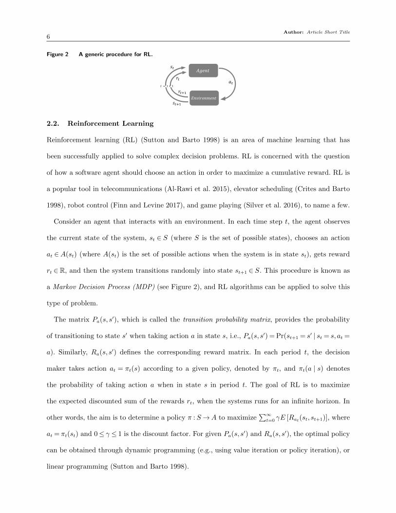
Figure 2 A generic procedure for RL.
𝐴𝑔𝑒𝑛𝑡
𝐸𝑛𝑣𝑖𝑟𝑜𝑛𝑚𝑒𝑛𝑡
𝑎𝑡
𝑟𝑡+1
𝑠𝑡+1
𝑟𝑡
𝑠𝑡
𝑡 = 𝑡 + 1
2.2. Reinforcement Learning
Reinforcement learning (RL) (Sutton and Barto 1998) is an area of machine learning that has
been successfully applied to solve complex decision problems. RL is concerned with the question
of how a software agent should choose an action in order to maximize a cumulative reward. RL is
a popular tool in telecommunications (Al-Rawi et al. 2015), elevator scheduling (Crites and Barto
1998), robot control (Finn and Levine 2017), and game playing (Silver et al. 2016), to name a few.
Consider an agent that interacts with an environment. In each time step t, the agent observes
the current state of the system, st ∈ S (where S is the set of possible states), chooses an action
at ∈A(st) (where A(st) is the set of possible actions when the system is in state st), gets reward
rt ∈R, and then the system transitions randomly into state st+1 ∈ S. This procedure is known as
a Markov Decision Process (MDP) (see Figure 2), and RL algorithms can be applied to solve this
type of problem.
The matrix Pa(s, s′), which is called the transition probability matrix, provides the probability
of transitioning to state s′ when taking action a in state s, i.e., Pa(s, s′) = Pr(st+1 = s′ | st = s, at =
a). Similarly, Ra(s, s′) defines the corresponding reward matrix. In each period t, the decision
maker takes action at = πt(s) according to a given policy, denoted by πt, and πt(a | s) denotes
the probability of taking action a when in state s in period t. The goal of RL is to maximize
the expected discounted sum of the rewards rt, when the systems runs for an infinite horizon. In
other words, the aim is to determine a policy π : S→A to maximize∑∞
t=0 γE [Rat(st, st+1)], where
at = πt(st) and 0≤ γ ≤ 1 is the discount factor. For given Pa(s, s′) and Ra(s, s
′), the optimal policy
can be obtained through dynamic programming (e.g., using value iteration or policy iteration), or
linear programming (Sutton and Barto 1998).
Author: Article Short Title7
Another approach for solving this problem is Q-learning, a type of RL algorithm that obtains
the policy π that maximizes the Q-value for any s∈ S and a= π(s), i.e.:
Q(s, a) = maxπE[rt + γrt+1 + γ2rt+2 + · · · | st = s, at = a,π
]. (2)
The Q-learning approach starts with an initial guess for Q(s, a) for all s and a and then proceeds
to update them based on the iterative formula
Q(st, at) = (1−αt)Q(st, at) +αt
(rt+1 + γmax
aQ(st+1, a)
),∀t= 1,2, . . . , (3)
where αt is the learning rate at time step t. In each observed state, the agent chooses an action
through an ε-greedy algorithm: with probability εt in time t, the algorithm chooses an action
randomly, and with probability 1− εt, it chooses the action with the highest cumulative action
value, i.e., at+1 = argmaxaQ(st+1, a). The random selection of actions, called exploration, allows
the algorithm to explore the solution space more fully and gives an optimality guarantee to the
algorithm if εt→ 0 when t→∞ (Sutton and Barto 1998).
All of the algorithms discussed so far guarantee that they will obtain the optimal policy. However,
due to the curse of dimensionality, these approaches are not able to solve MDPs with large state or
action spaces in reasonable amounts of time. Many problems of interest (including the beer game)
have large state and/or action spaces. Moreover, in some settings (again, including the beer game),
the decision maker cannot observe the full state variable. This case, which is known as a partially
observed MDP (POMDP), makes the problem much harder to solve than MDPs.
In order to solve large POMDPs and avoid the curse of dimensionality, it is common to approxi-
mate the Q-values in the Q-learning algorithm (Sutton and Barto 1998). Linear regression is often
used for this purpose (Melo and Ribeiro 2007); however, it is not powerful or accurate enough
for our application. Non-linear functions and neural network approximators are able to provide
more accurate approximations; on the other hand, they are known to provide unstable or even
diverging Q-values due to issues related to non-stationarity and correlations in the sequence of
observations (Mnih et al. 2013). The seminal work of Mnih et al. (2015) solved these issues by
Author: Article Short Title8
proposing target networks and utilizing experience replay memory (Lin 1992). They proposed a
deep Q-network (DQN) algorithm, which uses a deep neural network to obtain an approximation
of the Q-function, and trains it through the iterations of the Q-learning algorithm while updating
another target network. This algorithm has been applied to many competitive games, which are
reviewed by Li (2017). Our algorithm for the beer game is based on this approach.
The beer game exhibits one more characteristic that differentiates it from most settings in which
DQN is commonly applied, namely, that there are multiple agents that cooperate in a decentralized
manner to achieve a common goal. Such a problem is called a decentralized POMDP, or Dec-
POMDP. Due to the partial observability and the non-stationarity of the local observations of each
agent, Dec-POMDPs are extremely hard to solve and are categorized as NEXP-complete problems
(Bernstein et al. 2002).
The beer game exhibits all of the complicating characteristics described above—large state and
action spaces, partial state observations, and decentralized cooperation. In the next section, we
discuss the drawbacks of current approaches for solving the beer game, which our algorithm aims
to overcome.
2.3. Drawbacks of Current Algorithms
In Section 2.1, we reviewed different approaches to solve the beer game. Although the model of
Clark and Scarf (1960) can solve some types of serial systems, for more general serial systems
neither the form nor the parameters of the optimal policy are known. Moreover, even in systems
for which a base-stock policy is optimal, such a policy may no longer be optimal for a given agent
if the other agents do not follow it. The formula-based beer-game models by Mosekilde and Larsen
(1988), Sterman (1989), and Strozzi et al. (2007) attempt to model human decision-making; they
do not attempt to model or determine optimal decisions.
A handful of models have attempted to optimize the inventory actions in serial supply chains
with more general cost or demand structures than those used by Clark and Scarf (1960); these are
essentially beer-game settings. However, these papers all assume full observation or a centralized
Author: Article Short Title9
decision maker, rather than the local observations and decentralized approach taken in the beer
game. For example, Kimbrough et al. (2002) use a genetic algorithm (GA), while Chaharsooghi
et al. (2008), Giannoccaro and Pontrandolfo (2002) and Jiang and Sheng (2009) use RL. However,
classical RL algorithms can handle only a small or reduced-size state space. Accordingly, these
applications of RL in the beer game or even simpler supply chain networks also assume (implicitly
or explicitly) that size of the state space is small. This is unrealistic in the beer game, since the
state variable representing a given agent’s inventory level can be any number in (−∞,+∞). Solving
such an RL problem would be nearly impossible, as the model would be extremely expensive
to train. Moreover, Chaharsooghi et al. (2008) and Giannoccaro and Pontrandolfo (2002), which
model beer-game-like settings, assume sharing of information, which is not the typical assumption
in the beer game. Also, to handle the curse of dimensionality, they propose mapping the state
variable onto a small number of tiles, which leads to the loss of valuable state information and
therefore of accuracy. Thus, although these papers are related to our work, their assumption of full
observability differentiates their work from the classical beer game and from our paper.
As we discussed in Section 2.2, the beer game is a Dec-POMDP. The algorithm proposed by Xuan
et al. (2004) for general Dec-POMDPs cannot be used for the beer game since they allow agents
to communicate, with some penalty; without the communication, there is no way for the agents
to learn the shared objective function. Similarly, Seuken and Zilberstein (2007) and Omidshafiei
et al. (2017) propose algorithms to solve multi-agent problems under partial observability while
assuming there is a reward shared by all agents that is known by all agents in every period, but in
the beer game the agents do not learn the full reward until the game ends. For a survey of research
on ILs with shared rewards, see Matignon et al. (2012).
Another possible approach to tackle this problem might be classical supervised machine learning
algorithms. However, these algorithms also cannot be readily applied to the beer game, since there
is no historical data in the form of “correct” input/output pairs. Thus, we cannot use a stand-alone
support vector machine or deep neural network with a training data-set and train it to learn the
Author: Article Short Title10
best action (like the approach used by Oroojlooyjadid et al. (2017a,b) to solve some simpler supply
chain problems). Based on our understanding of the literature, there is a large gap between solving
the beer game problem effectively and what the current algorithms can handle. In order to fill this
gap, we propose a variant of the DQN algorithm to choose the order quantities in the beer game.
2.4. Our Contribution
We propose a Q-learning algorithm for the beer game in which a DNN approximates the Q-function.
Indeed, the general structure of our algorithm is based on the DQN algorithm (Mnih et al. 2015),
although we modify it substantially, since DQN is formulated for single-agent, competitive, zero-
sum games and the beer game is a multi-agent, decentralized, cooperative, non-zero-sum game.
In other words, DQN provides actions for one agent that interacts with an environment in a
competitive setting, and the beer game is a cooperative game in the sense that all of the players aim
to minimize the total cost of the system in a random number of periods. Also, beer game agents
are playing independently and do not have any information from other agents until the game ends
and the total cost is revealed, whereas DQN usually assumes the agent fully observes the state of
the environment at any time step t of the game. For example, DQN has been successfully applied
to Atari games (Mnih et al. 2015), Go (Silver et al. 2016), and chess (Silver et al. 2017), but in
these games the agent is attempting to defeat an opponent (human or computer) and observes full
information about the state of the systems at each time step t.
One naive approach to extend the DQN algorithm to solve the beer game is to use multiple
DQNs, one to control the actions of each agent. However, using DQN as the decision maker of each
agent results in a competitive game in which each DQN agent plays independently to minimize
its own cost. For example, consider a beer game in which players 2, 3, and 4 each have a stand-
alone, well-trained DQN and the retailer (stage 1) uses a base-stock policy to make decisions. If
the holding costs are positive for all players and the stockout cost is positive only for the retailer
(as is common in the beer game), then the DQN at agents 2, 3, and 4 will return an optimal order
quantity of 0 in every period, since on-hand inventory hurts the objective function for these players,

Author: Article Short Title11
but stockouts do not. This is a byproduct of the independent DQN agents minimizing their own
costs without considering the total cost, which is obviously not an optimal solution for the system
as a whole.
Instead, we propose a unified framework in which the agents still play independently from one
another, but in the training phase, we use a feedback scheme so that the DQN agent learns the
total cost for the whole network and can, over time, learn to minimize it. Thus, the agents in our
model play smartly in all periods of the game to get a near-optimal cumulative cost for any random
horizon length.
In principle, our framework can be applied to multiple DQN agents playing the beer game
simultaneously on a team. However, to date we have designed and tested our approach only for a
single DQN agent whose teammates are not DQNs, e.g., they are controlled by simple formulas or
by human players. Enhancing the algorithm so that multiple DQNs can play simultaneously and
cooperatively is a topic of ongoing research.
Another advantage of our approach is that it does not require knowledge of the demand distri-
bution, unlike classical inventory management approaches (e.g., Clark and Scarf 1960). In practice,
one can approximate the demand distribution based on historical data, but doing so is prone to
error, and basing decisions on approximate distributions may result in loss of accuracy in the beer
game. In contrast, our algorithm chooses actions directly based on the training data and does not
need to know, or estimate, the probability distribution directly.
The proposed approach works very well when we tune and train the DQN for a given agent
and a given set of game parameters (e.g., costs, lead times, and action spaces). Once any of these
parameters changes, or the agent changes, in principle we need to tune and train a new network.
Although this approach works, it is time consuming since we need to tune hyper-parameters for
each new set of game parameters. To avoid this, we propose using a transfer learning (Pan and
Yang 2010) approach in which we transfer the acquired knowledge of one agent under one set of
game parameters to another agent with another set of game parameters. In this way, we decrease
the required time to train a new agent by roughly one order of magnitude.
Author: Article Short Title12
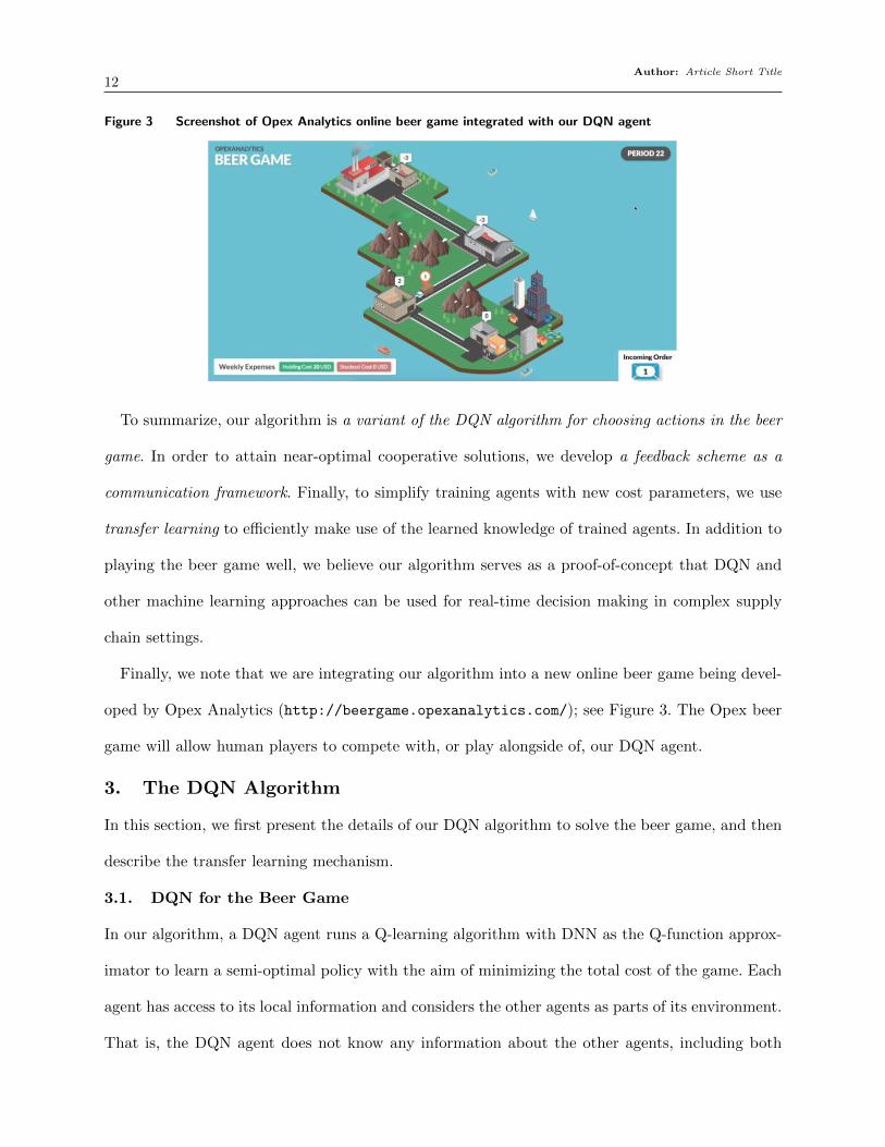
Figure 3 Screenshot of Opex Analytics online beer game integrated with our DQN agent
To summarize, our algorithm is a variant of the DQN algorithm for choosing actions in the beer
game. In order to attain near-optimal cooperative solutions, we develop a feedback scheme as a
communication framework. Finally, to simplify training agents with new cost parameters, we use
transfer learning to efficiently make use of the learned knowledge of trained agents. In addition to
playing the beer game well, we believe our algorithm serves as a proof-of-concept that DQN and
other machine learning approaches can be used for real-time decision making in complex supply
chain settings.
Finally, we note that we are integrating our algorithm into a new online beer game being devel-
oped by Opex Analytics (http://beergame.opexanalytics.com/); see Figure 3. The Opex beer
game will allow human players to compete with, or play alongside of, our DQN agent.
3. The DQN Algorithm
In this section, we first present the details of our DQN algorithm to solve the beer game, and then
describe the transfer learning mechanism.
3.1. DQN for the Beer Game
In our algorithm, a DQN agent runs a Q-learning algorithm with DNN as the Q-function approx-
imator to learn a semi-optimal policy with the aim of minimizing the total cost of the game. Each
agent has access to its local information and considers the other agents as parts of its environment.
That is, the DQN agent does not know any information about the other agents, including both
Author: Article Short Title13
static parameters such as costs and lead times, as well as dynamic state variables such as inventory
levels. We propose a feedback scheme to teach the DQN agent to work toward minimizing the total
system-wide cost, rather than its own local cost. The details of the scheme, Q-learning, state and
action spaces, reward function, DNN approximator, and the DQN algorithm are discussed below.
State variables: Consider agent i in time step t. Let OOit denote the on-order items at agent i,
i.e., the items that have been ordered from agent i+ 1 but not received yet; let dit denote the size
of the demand/order received from agent i− 1; let RSit denote the size of the shipment received
from agent i+ 1; let ait denote the action agent i takes; and let ILit denote the inventory level as
defined in Section 1. We interpret d0t to represent the end-customer demand and RS5t to represent
the shipment received by agent 4 from the external supplier. In each period t of the game, agent
i observes ILit, OOit, d
it, and RSit . In other words, in period t agent i has historical observations
oit = [(ILi1,OOi1, d
i1,RS
i1, a
i1), . . . , (IL
it,OO
it, d
it,RS
it , a
it)] , and does not have any information about
the other agents. Thus, the agent has to make its decision with partially observed information of
the environment. In addition, any beer game will finish in a finite time horizon, so the problem
can be modeled as a POMDP in which each historic sequence oit is a distinct state and the size
of the vector oit grows over time, which is difficult for the any RL and DNN algorithm to handle.
To address this issue, we capture only the last m periods (e.g., m= 3) and use them as the state
variable; thus the state variable of agent i in time t is sit =[(ILij,OO
ij, d
ij,RS
ij, a
ij)]tj=t−m+1
.
DNN architecture: In our algorithm, DNN plays the role of the Q-function approximator, pro-
viding the Q-value as output for any pair of state s and action a. There are various possible
approaches to build the DNN structure. One natural approach is to provide the state s and action
a as the input of the DNN and then get the corresponding Q(s, a) from the output. Another
approach is to include the state s in the DNN’s input and get the corresponding Q-value of all
possible actions in the DNN’s output so that the DNN output is of size |A|. The first approach
requires more, but smaller, DNN networks, while the second requires fewer, larger ones. We have
found that the second approach is much more efficient in the sense that it requires less training

Author: Article Short Title14
overall (even though the network is larger), so we use this approach in our algorithm. Thus, we
provide as input the m previous state variables into the DNN and get as output Q(s, a) for every
possible action a∈A(s).
Action space: In each period of the game, each agent can order any amount in [0,∞). Since our
DNN architecture provides the Q-value of all possible actions in the output, having an infinite
action space is not practical. Therefore, to limit the cardinality of the action space, we use the
d+ x rule for selecting the order quantity: The agent determines how much more or less to order
than its received order; that is, the order quantity is d+x, where x is in some bounded set. Thus,
the output of the DNN is x∈ [al, au] (al, au ∈Z), so that the action space is of size |au− al + 1|.
Experience replay: The DNN algorithm requires a mini-batch of input and a corresponding set
of output values to learn the Q-values. Since we use a Q-learning algorithm as our RL engine, we
have information about the new state st+1 along with information about the current state st, the
action at taken, and the observed reward rt, in each period t. This information can provide the
required set of input and output for the DNN; however, the resulting sequence of observations from
the RL results in a non-stationary data-set in which there is a strong correlation among consecutive
records. This makes the DNN and, as a result, the RL prone to over-fitting the previously observed
records and may even result in a diverging approximator (Mnih et al. 2015). To avoid this problem,
we follow the suggestion of Mnih et al. (2015) and use experience replay (Lin 1992), taking a mini-
batch from it in every training step. In this way, agent i has experience memory Ei, which holds
the previously seen states, actions taken, corresponding rewards, and new observed states. Thus,
in iteration t of the algorithm, agent i’s observation eit = (sit, ait, r
it, s
it+1) is added to the experience
memory of the agent so that Ei includes {ei1, ei2, . . . , eit} in period t. Then, in order to avoid having
correlated observations, we select a random mini-batch of the agent’s experience replay to train the
corresponding DNN (if applicable). This approach breaks the correlations among the training data
and reduces the variance of the output (Mnih et al. 2013). Moreover, as a byproduct of experience
replay, we also get a tool to keep every piece of the valuable information, which allows greater
Author: Article Short Title15
efficiency in a setting in which the state and action spaces are huge and any observed experience is
valuable. However, in our implementation of the algorithm we keep only the last M observations
due to memory limits.
Reward function: In iteration t of the game, agent i observes state variable sit and takes action
ait; we need to know the corresponding reward value rit to measure the quality of action ait. The
state variable, sit+1, allows us to calculate ILit+1 and thus the corresponding shortage or holding
costs, and we consider the summation of these costs for rit. However, since there are information
and transportation lead times, there is a delay between taking action ait and observing its effect on
the reward. Moreover, the reward rit reflects not only the action taken in period t, but also those
taken in previous periods, and it is not possible to decompose rit to isolate the effects of each of
these actions. However, defining the state variable to include information from the last m periods
resolves this issue; the reward rit represents the reward of state sit, which includes the observations
of the previous m steps.
On the other hand, the reward values rit are the intermediate rewards of each agent, and the
objective of the beer game is to minimize the total reward of the game,∑4
i=1
∑T
t=1 rit, which
the agents only learn after finishing the game. In order to add this information into the agents’
experience, we revise the reward of the relevant agents in all T time steps through a feedback
scheme.
Feedback scheme: When any episode of the beer game is finished, all agents are made aware of
the total reward. In order to share this information among the agents, we propose a penalization
procedure in the training phase to provide feedback to the DQN agent about the way that it has
played. Let ω=∑4
i=1
∑T
t=1ritT
and τ i =∑T
t=1ritT
, i.e., the average reward per period and the average
reward of agent i per period, respectively. After the end of each episode of the game (i.e., after
period T ), for each DQN agent i we update its observed reward in all T time steps in the experience
replay memory using rit = rit +βi3
(ω− τ i), ∀t∈ {1, . . . , T}, where βi is a regularization coefficient for
agent i. With this procedure, agent i gets appropriate feedback about its actions and learns to take
Author: Article Short Title16
actions that result in minimum total cost, not locally optimal solutions. This feedback scheme gives
the agents a sort of implicit communication mechanism, even though they do not communicate
directly.
Determining the value of m: As noted above, the DNN maintains information from the most
recent m periods in order to keep the size of the state variable fixed and to address the issue with the
delayed observation of the reward. In order to select an appropriate value for m, one has to consider
the value of the lead times throughout the game. First, when agent i takes a given action ait at time
t, it does not observe its effect until at least ltri + lfii periods later, when the order may be received.
Moreover, node i+1 may not have enough stock to satisfy the order immediately, in which case the
shipment is delayed and in the worst case agent i will not observe the corresponding reward rit until∑4
j=i(ltrj + lfij ) periods later. However, the Q-learning algorithm needs the reward rit to evaluate the
action ait taken. Thus, ideally m should be chosen at least as large as∑4
j=1(ltrj + lfij ). On the other
hand, selecting such a large value for m results in a large input size for the DNN, which increases
the training time. Therefore, selecting m is a trade-off between accuracy and computation time,
and m should be selected according to the required level of accuracy and the available computation
power. In our numerical experiment,∑4
j=1(ltrj + lfij ) = 16, and we test m∈ {5,10}.
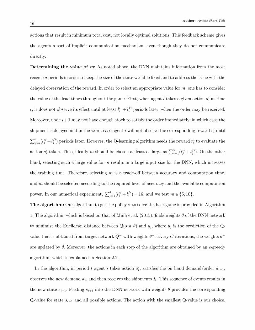
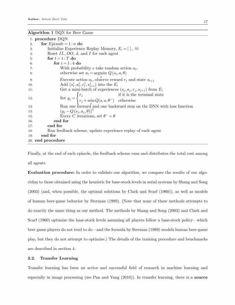
The algorithm: Our algorithm to get the policy π to solve the beer game is provided in Algorithm
1. The algorithm, which is based on that of Mnih et al. (2015), finds weights θ of the DNN network
to minimize the Euclidean distance between Q(s, a, θ) and yj, where yj is the prediction of the Q-
value that is obtained from target network Q− with weights θ−. Every C iterations, the weights θ−
are updated by θ. Moreover, the actions in each step of the algorithm are obtained by an ε-greedy
algorithm, which is explained in Section 2.2.
In the algorithm, in period t agent i takes action ait, satisfies the on hand demand/order dt−1,
observes the new demand dt, and then receives the shipments It. This sequence of events results in
the new state st+1. Feeding st+1 into the DNN network with weights θ provides the corresponding
Q-value for state st+1 and all possible actions. The action with the smallest Q-value is our choice.
Author: Article Short Title17
Algorithm 1 DQN for Beer Game
1: procedure DQN2: for Episode= 1 : n do3: Initialize Experience Replay Memory, Ei = [ ] , ∀i4: Reset IL, OO, d, and I for each agent5: for t= 1 : T do6: for i= 1 : 4 do7: With probability ε take random action at,8: otherwise set at = argmin
aQ (st, a, θ)
9: Execute action at, observe reward rt and state st+1
10: Add (s1t , a1t , r
1t , s
1t+1) into the Ei
11: Get a mini-batch of experiences (sj, aj, rj, sj+1) from Ei
12: Set yj =
{rj if it is the terminal state
rj + minaQ(s, a, θ−) otherwise
13: Run one forward and one backward step on the DNN with loss function14: (yj −Q (sj, aj, θ))
2
15: Every C iterations, set θ− = θ16: end for17: end for18: Run feedback scheme, update experience replay of each agent19: end for20: end procedure
Finally, at the end of each episode, the feedback scheme runs and distributes the total cost among
all agents.
Evaluation procedure: In order to validate our algorithm, we compare the results of our algo-
rithm to those obtained using the heuristic for base-stock levels in serial systems by Shang and Song
(2003) (and, when possible, the optimal solutions by Clark and Scarf (1960)), as well as models
of human beer-game behavior by Sterman (1989). (Note that none of these methods attempts to
do exactly the same thing as our method. The methods by Shang and Song (2003) and Clark and
Scarf (1960) optimize the base-stock levels assuming all players follow a base-stock policy—which
beer game players do not tend to do—and the formula by Sterman (1989) models human beer-game
play, but they do not attempt to optimize.) The details of the training procedure and benchmarks
are described in section 4.
3.2. Transfer Learning
Transfer learning has been an active and successful field of research in machine learning and
especially in image processing (see Pan and Yang (2010)). In transfer learning, there is a source

Author: Article Short Title18
dataset S and a trained neural network to perform a given task, e.g. classification, regression, or
decisioning through RL. Training such networks may take a few days or even weeks. So, for similar
or even slightly different target datasets T, one can avoid training a new network from scratch
and instead use the same trained network with a few customizations. The idea is that most of the
learned knowledge on dataset S can be used in the target dataset with a small amount of additional
training. This idea works well in image processing (e.g. Sharif Razavian et al. (2014), Rajpurkar
et al. (2017)) and considerably reduces the training time.
In order to use transfer learning in the beer game, we first train a fixed-size network for a given
agent i ∈ {1,2,3,4} with a given set of game parameters P i1 = {|Ai1(s)|, cip1 , cih1}. (P i
1 includes the
size of agent i’s action space as well as its costs, but in principle one could also include lead times
and other game parameters.) Assume that we wish to apply this learned knowledge to other agents,
with other game parameters. For those agents, we construct a new DNN network in which the
input values, as well as the learned weights in the first layer, are similar to the values from the fully
trained agent, i. As we get closer to the final layer, which provides the Q-values, the weights become
less similar to agent i’s and more specific to each agent. Thus, similar to the idea of Sharif Razavian
et al. (2014) and Rajpurkar et al. (2017), the acquired knowledge in the first k hidden layer(s) of
the neural network belongs to agent i and is transferred to agent j, with P j2 6= P i
1, where k is a
tunable parameter.
To be more precise, assume there exists a source agent i ∈ {1,2,3,4} with trained network Si
and parameters P i1 = {|Aj1(s)|, cjp1 , c
jh1}. Weight matrix Wi contains the learned weights such that
W qi denotes the weight between layers q and q + 1 of the neural network, where q ∈ {0, . . . , nh},
and nh is the number of hidden layers. The aim is to train a neural network Sj for target agent
j ∈ {1,2,3,4}, j 6= i. We set the structure of the network Sj the same as that of Si, and initialize
Wj with Wi, making the first k layers not trainable. Then, we train neural network Sj with a small
learning rate.
In Section 4.3, we test the use of transfer learning in four cases:
Author: Article Short Title19
1. Transfer the learned knowledge of source agent i to target agent j 6= i in the same game.
2. Transfer the learned knowledge of source agent i to target agent j with {|Aj1(s)|, cjp2 , cjh2}, i.e.,
the same action space but different cost coefficients.
3. Transfer the learned knowledge of source agent i to target agent j with {|Aj2(s)|, cjp1 , cjh1}, i.e.,
the same cost coefficients but different action space.
4. Transfer the learned knowledge of source agent i to target agent j with {|Aj2(s)|, cjp2 , cjh2}, i.e.,
different action space and cost coefficients.
Transfer learning could also be used when other aspects of the problem change, e.g., lead times,
demand distributions, and so on. This avoids having to to tune the parameters of the neural
network for each new problem, which considerably reduces the training time. However, we still
need to decide how many layers should be trainable, as well as to determine which agent can be a
base agent for transferring the learned knowledge. Still, this is computationally much cheaper than
finding each network and its hyper-parameters from scratch.
4. Numerical Experiments
We test our approach using a beer game setup with the following characteristics. Information and
shipment lead times are two periods each at every agent. Holding and stockout costs are equal
to ch = [2,2,2,2] and cp = [2,0,0,0], respectively, where the vectors specify the values for agents
1, . . . ,4. The demand is an integer uniformly drawn from {0,1,2}. (This can be thought of as
similar to Sterman’s original beer game setup, in which the demands are 4 or 8, except that ours
are divided by 4 and are random.) The rewards (costs) are normalized by dividing them by 200,
which helps to reduce the loss function values and produce smaller gradients. We test values of m
in {5,10}. (Recall that m is the number of periods of history that are stored in the state variable.)
In most of our computational results, we use al =−2 and au = 2; i.e., each agent chooses an order
quantity that is at most 2 units greater or less than the observed demand. (Later, we expand this
to 5.)
Our DNN network is a fully connected network, in which each node has a ReLU activation
function. The input is of size 5m, and the number of hidden layers is randomly selected as either

Author: Article Short Title20
2 or 3 (with equal probability). There is one output node for each possible value of the action,
and each of these nodes takes a value in R indicating the Q-value for that action. Thus, there are
au − al + 1 output nodes, which for us equals 5 since al =−2 and au = 2. When the network has
two hidden layers, its shape is [5m,130,90,5], and with three hidden layers it is [5m,130,90,50,5].
In order to optimize the network, we used the Adam optimizer (Kingma and Ba 2014) with a
batch size of 64. Although the Adam optimizer has its own weight decaying procedure, we used
exponential decay with a stair of 10000 iterations with rate 0.98 to decay the learning rate further.
We trained each agent on 40000 episodes and used a replay memory of the one million most recently
observed experiences. Also, the training of the DNN starts after observing at least 500 episodes of
the game. The ε-greedy algorithm starts with ε= 0.9 and linearly reduces it to 0.1 in the first 80%
of iterations. All of the computations are done on nodes with 16 cores and 32 GB of memory with
TensorFlow 1.4 (Abadi et al. 2015).
In the feedback mechanism, the appropriate value of the feedback coefficient βi heavily depends
on τj, the average reward for agent j, for each j 6= i. For example, when τi is one order of magnitude
larger than τj, for all j 6= i, agent i needs a large coefficient to get more feedback from the other
agents. Indeed, the feedback coefficient has a similar role as the regularization parameter λ has in
the lasso loss function; the value of that parameter depends on the `-norm of the variables, but
there is no universal rule to determine the best value for λ. Similarly, proposing a simple rule or
value for each βi is not possible, as it depends on τi, ∀i. For example, we found that a very large
βi does not work well, since the agent tries to decrease other agents’ costs rather than its own.
Similarly, with a very small βi, the agent learns how to minimize its own cost instead of the total
cost. Therefore, we used a similar cross validation approach to find good values for each βi.
As noted above, we only consider cases in which a single DQN plays with non-DQN agents, e.g.,
simulated human players. We consider two types of simulated human players. In Section 4.1, we
discuss results for the case in which one DQN agent plays on a team in which the other three
players use a base-stock policy to choose their actions, i.e., the non-DQN agents behave rationally.
Author: Article Short Title21
See https://youtu.be/gQa6iWGcGWY for a video animation of the policy that the DQN learns in
this case. Then, in Section 4.2, we assume that the other three agents use the Sterman formula
(i.e., the anchoring-and-adjustment formula by Sterman (1989)), which models irrational play.
For the cost coefficients and other settings specified for our beer game, it is optimal for all players
to follow a base-stock policy, and we use this policy (with the optimal parameters as determined
by the method of Clark and Scarf (1960)) as a benchmark and a lower bound on the base stock
cost. The vector of base-stock levels is [9,5,3,1], and the resulting average cost per period is 2.008,
though these levels may be slightly suboptimal due to rounding. This cost is allocated to stages 1–4
as [1.91,0.05,0.02,0.03], i.e., the retailer bears the most significant share of the total cost. In the
experiments in which one of the four agents is played by the DQN, the other three agents continue
to use their optimal base-stock levels.
Finally, in Section 4.3 we provide the results obtained using transfer learning, for cases in which
there is a DQN player with three other agents, each following a base-stock policy.
4.1. DQN Plus Base-Stock Policy
In this section, we present the results of our algorithm when the other three agents use a base-stock
policy. We consider four cases, with the DQN playing the role of each of the four players and the
other three agents using a base-stock policy. We then compare the results of our algorithm with
the results of the case in which all players follow the base-stock policy, which we call BS hereinafter.
The results of all four cases are shown in Figure 4. Each plot shows the training curve, i.e., the
evolution of the average cost per game as the training progresses. In particular, the horizontal axis
indicates the number of training episodes, while the vertical axis indicates the total cost per game.
After every 100 episodes of the game and the corresponding training, the cost of 50 validation
points (i.e., 50 new games) are obtained and their average is plotted. The red line indicates the cost
of the case in which all players follow a base-stock policy. In each of the sub-figures, there are two
plots; the upper plot shows the cost, while the lower plot shows the normalized cost, in which each
cost is divided by the corresponding BS cost; essentially this is a “zoomed-in” version of the upper
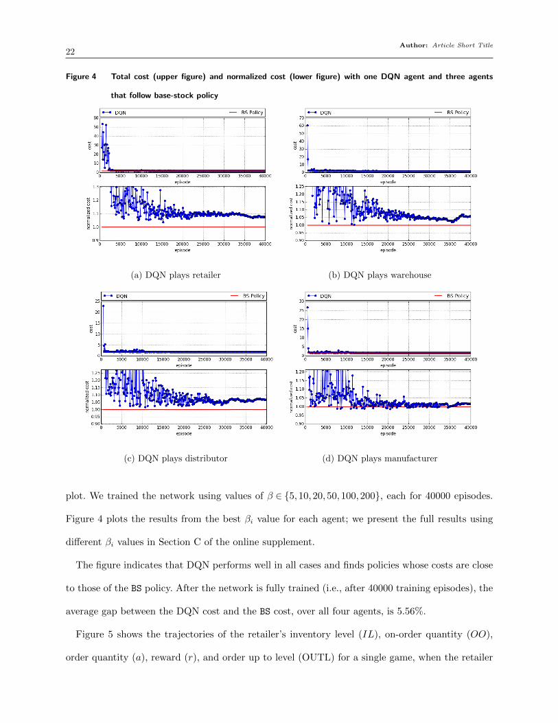
Author: Article Short Title22
Figure 4 Total cost (upper figure) and normalized cost (lower figure) with one DQN agent and three agents
that follow base-stock policy
(a) DQN plays retailer (b) DQN plays warehouse
(c) DQN plays distributor (d) DQN plays manufacturer
plot. We trained the network using values of β ∈ {5,10,20,50,100,200}, each for 40000 episodes.
Figure 4 plots the results from the best βi value for each agent; we present the full results using
different βi values in Section C of the online supplement.
The figure indicates that DQN performs well in all cases and finds policies whose costs are close
to those of the BS policy. After the network is fully trained (i.e., after 40000 training episodes), the
average gap between the DQN cost and the BS cost, over all four agents, is 5.56%.
Figure 5 shows the trajectories of the retailer’s inventory level (IL), on-order quantity (OO),
order quantity (a), reward (r), and order up to level (OUTL) for a single game, when the retailer

Author: Article Short Title23
Figure 5 ILt, OOt, at, rt, and OUTL when DQN plays retailer and other agents follow base-stock policy
is played by the DQN with β1 = 50, as well as when it is played by a base-stock policy (BS), and
the Sterman formula (Strm). The base-stock policy and DQN have similar IL and OO trends, and
as a result their rewards are also very close: BS has a cost of [1.42,0.00,0.02,0.05] (total 1.49) and
DQN has [1.43,0.01,0.02,0.08] (total 1.54, or 3.4% larger). (Note that BS has a slightly different
cost here than reported on page 21 because those costs are the average costs of 50 samples while
this cost is from a single sample.) Similar trends are observed when the DQN plays the other three
roles; see Section A of the online supplement. This suggests that the DQN can successfully learn
to achieve costs close to BS when the other agents also play BS. (The OUTL plot shows that the
DQN does not quite follow a base-stock policy, even though its costs are similar.)
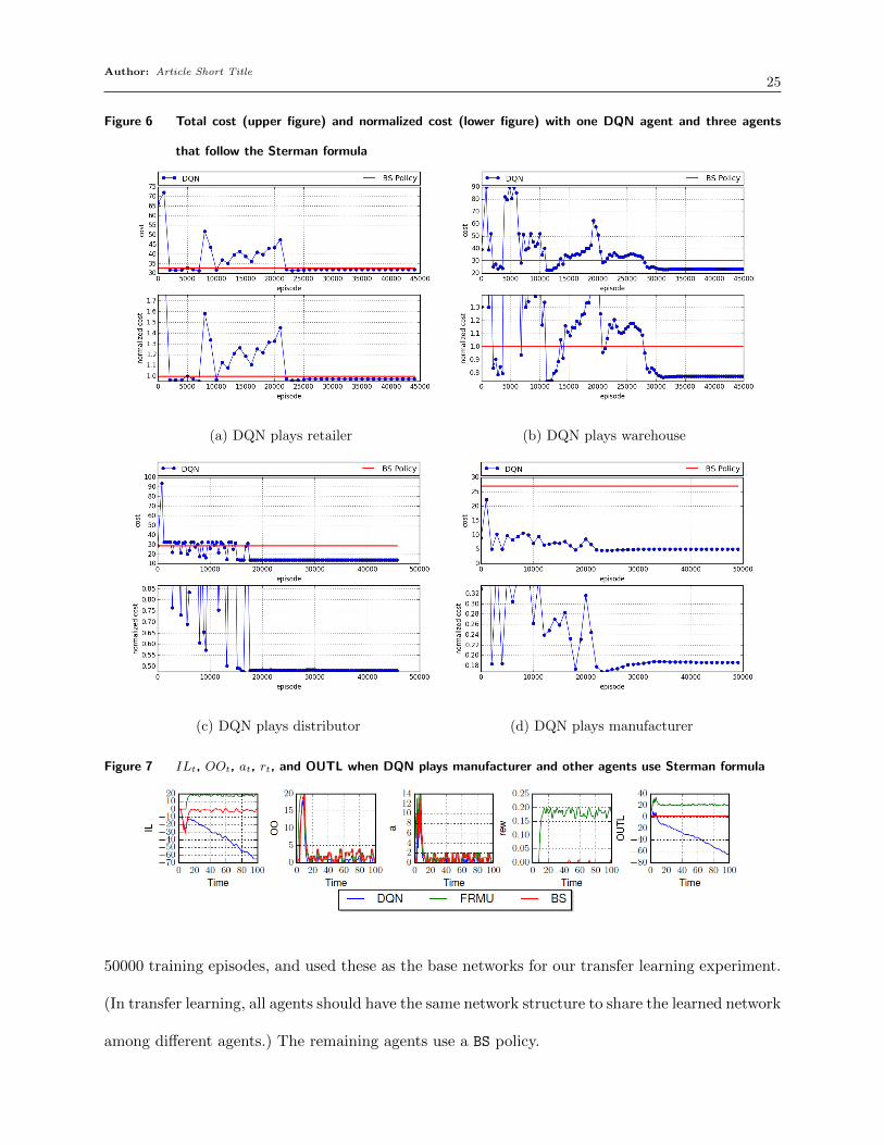
4.2. DQN Plus Sterman Formula
Figure 6 shows the results of the case in which the three non-DQN agents use the formula proposed
by Sterman (1989) instead of a base-stock policy. (See Section B of online supplement for the
formula and its parameters.) We train the network using values of β ∈ {1,2,5,10,20,50,75,100},
each for 40000 episodes, and report the best result among them. For comparison, the red line
represents the case in which the single agent is played using a base-stock policy and the other three
agents continue to use the Sterman formula, a case we call Strm-BS.
From the figure, it is evident that the DQN plays much better than Strm-BS. This is because if
the other three agents do not follow a base-stock policy, it is no longer optimal for the fourth agent
to follow a base-stock policy, or to use the same base-stock level. In general, the optimal inventory
policy when other agents do not follow a base-stock policy is an open question. This figure suggests
that our DQN is able to learn to play effectively in this setting.
Author: Article Short Title24
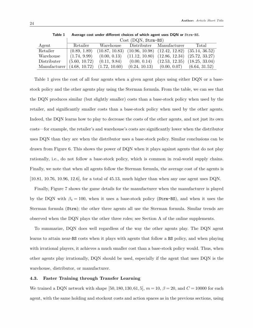
Table 1 Average cost under different choices of which agent uses DQN or Strm-BS.
Cost (DQN, Strm-BS)Agent Retailer Warehouse Distributer Manufacturer TotalRetailer (0.89, 1.89) (10.87, 10.83) (10.96, 10.98) (12.42, 12.82) (35.14, 36.52)Warehouse (1.74, 9.99) (0.00, 0.13) (11.12, 10.80) (12.86, 12.34) (25.72, 33.27)Distributer (5.60, 10.72) (0.11, 9.84) (0.00, 0.14) (12.53, 12.35) (18.25, 33.04)Manufacturer (4.68, 10.72) (1.72, 10.60) (0.24, 10.13) (0.00, 0.07) (6.64, 31.52)
Table 1 gives the cost of all four agents when a given agent plays using either DQN or a base-
stock policy and the other agents play using the Sterman formula. From the table, we can see that
the DQN produces similar (but slightly smaller) costs than a base-stock policy when used by the
retailer, and significantly smaller costs than a base-stock policy when used by the other agents.
Indeed, the DQN learns how to play to decrease the costs of the other agents, and not just its own
costs—for example, the retailer’s and warehouse’s costs are significantly lower when the distributor
uses DQN than they are when the distributor uses a base-stock policy. Similar conclusions can be
drawn from Figure 6. This shows the power of DQN when it plays against agents that do not play
rationally, i.e., do not follow a base-stock policy, which is common in real-world supply chains.
Finally, we note that when all agents follow the Sterman formula, the average cost of the agents is
[10.81, 10.76, 10.96, 12.6], for a total of 45.13, much higher than when any one agent uses DQN.
Finally, Figure 7 shows the game details for the manufacturer when the manufacturer is played
by the DQN with β4 = 100, when it uses a base-stock policy (Strm-BS), and when it uses the
Sterman formula (Strm); the other three agents all use the Sterman formula. Similar trends are
observed when the DQN plays the other three roles; see Section A of the online supplements.
To summarize, DQN does well regardless of the way the other agents play. The DQN agent
learns to attain near-BS costs when it plays with agents that follow a BS policy, and when playing
with irrational players, it achieves a much smaller cost than a base-stock policy would. Thus, when
other agents play irrationally, DQN should be used, especially if the agent that uses DQN is the
warehouse, distributor, or manufacturer.
4.3. Faster Training through Transfer Learning
We trained a DQN network with shape [50,180,130,61,5], m= 10, β = 20, and C = 10000 for each
agent, with the same holding and stockout costs and action spaces as in the previous sections, using
Author: Article Short Title25
Figure 6 Total cost (upper figure) and normalized cost (lower figure) with one DQN agent and three agents
that follow the Sterman formula
(a) DQN plays retailer (b) DQN plays warehouse
(c) DQN plays distributor (d) DQN plays manufacturer
Figure 7 ILt, OOt, at, rt, and OUTL when DQN plays manufacturer and other agents use Sterman formula
50000 training episodes, and used these as the base networks for our transfer learning experiment.
(In transfer learning, all agents should have the same network structure to share the learned network
among different agents.) The remaining agents use a BS policy.
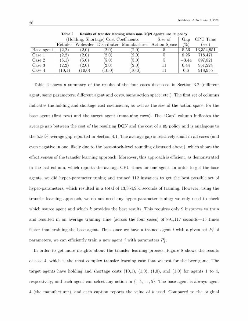
Author: Article Short Title26
Table 2 Results of transfer learning when non-DQN agents use BS policy
(Holding, Shortage) Cost Coefficients Size ofAction Space
Gap CPU TimeRetailer Wolesaler Distributer Manufacturer (%) (sec)
Base agent (2,2) (2,0) (2,0) (2,0) 5 5.56 13,354,951Case 1 (2,2) (2,0) (2,0) (2,0) 5 8.25 718,471Case 2 (5,1) (5,0) (5,0) (5,0) 5 −3.44 897,821Case 3 (2,2) (2,0) (2,0) (2,0) 11 6.44 951,224Case 4 (10,1) (10,0) (10,0) (10,0) 11 0.6 918,955
Table 2 shows a summary of the results of the four cases discussed in Section 3.2 (different
agent, same parameters; different agent and costs, same action space; etc.). The first set of columns
indicates the holding and shortage cost coefficients, as well as the size of the action space, for the
base agent (first row) and the target agent (remaining rows). The “Gap” column indicates the
average gap between the cost of the resulting DQN and the cost of a BS policy and is analogous to
the 5.56% average gap reported in Section 4.1. The average gap is relatively small in all cases (and
even negative in one, likely due to the base-stock-level rounding discussed above), which shows the
effectiveness of the transfer learning approach. Moreover, this approach is efficient, as demonstrated
in the last column, which reports the average CPU times for one agent. In order to get the base
agents, we did hyper-parameter tuning and trained 112 instances to get the best possible set of
hyper-parameters, which resulted in a total of 13,354,951 seconds of training. However, using the
transfer learning approach, we do not need any hyper-parameter tuning; we only need to check
which source agent and which k provides the best results. This requires only 9 instances to train
and resulted in an average training time (across the four cases) of 891,117 seconds—15 times
faster than training the base agent. Thus, once we have a trained agent i with a given set P i1 of
parameters, we can efficiently train a new agent j with parameters P j2 .
In order to get more insights about the transfer learning process, Figure 8 shows the results
of case 4, which is the most complex transfer learning case that we test for the beer game. The
target agents have holding and shortage costs (10,1), (1,0), (1,0), and (1,0) for agents 1 to 4,
respectively; and each agent can select any action in {−5, . . . ,5}. The base agent is always agent
4 (the manufacturer), and each caption reports the value of k used. Compared to the original
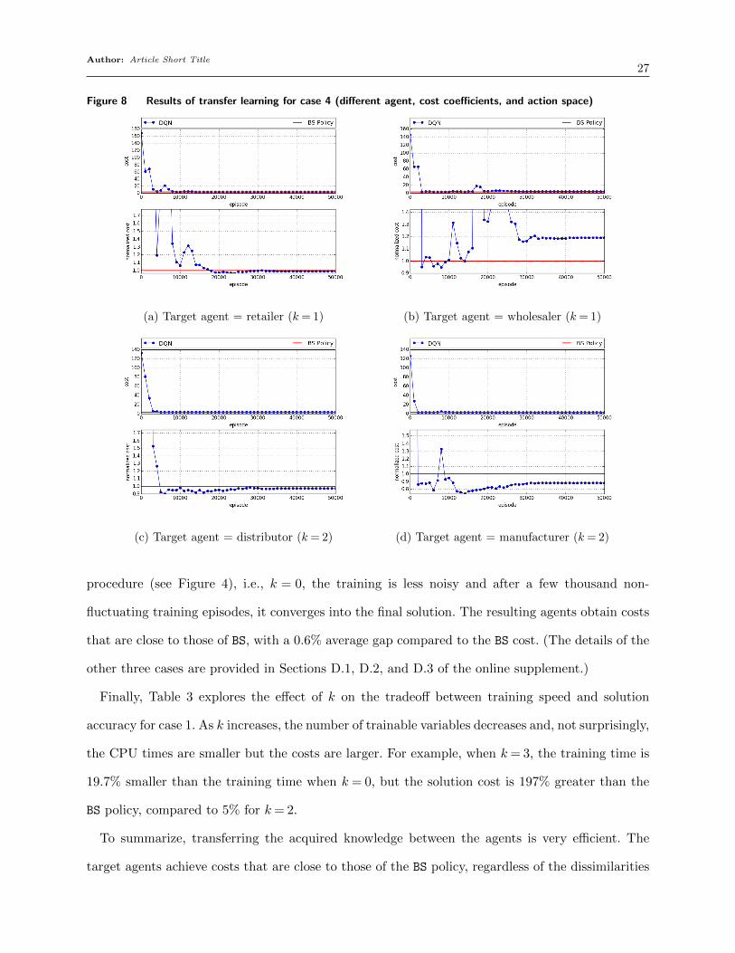
Author: Article Short Title27
Figure 8 Results of transfer learning for case 4 (different agent, cost coefficients, and action space)
(a) Target agent = retailer (k= 1) (b) Target agent = wholesaler (k= 1)
(c) Target agent = distributor (k= 2) (d) Target agent = manufacturer (k= 2)
procedure (see Figure 4), i.e., k = 0, the training is less noisy and after a few thousand non-
fluctuating training episodes, it converges into the final solution. The resulting agents obtain costs
that are close to those of BS, with a 0.6% average gap compared to the BS cost. (The details of the
other three cases are provided in Sections D.1, D.2, and D.3 of the online supplement.)
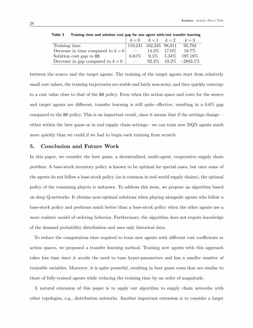
Finally, Table 3 explores the effect of k on the tradeoff between training speed and solution
accuracy for case 1. As k increases, the number of trainable variables decreases and, not surprisingly,
the CPU times are smaller but the costs are larger. For example, when k= 3, the training time is
19.7% smaller than the training time when k = 0, but the solution cost is 197% greater than the
BS policy, compared to 5% for k= 2.
To summarize, transferring the acquired knowledge between the agents is very efficient. The
target agents achieve costs that are close to those of the BS policy, regardless of the dissimilarities
Author: Article Short Title28
Table 3 Training time and solution cost gap for one agent with/out transfer learning
k= 0 k= 1 k= 2 k= 3Training time 119,241 102,335 98,911 95,793Decrease in time compared to k= 0 — 14.2% 17.0% 19.7%Solution cost gap vs BS 6.61% 0.5% 5.34% 197.18%Decrease in gap compared to k= 0 — 92.4% 19.2% −2883.1%
between the source and the target agents. The training of the target agents start from relatively
small cost values, the training trajectories are stable and fairly non-noisy, and they quickly converge
to a cost value close to that of the BS policy. Even when the action space and costs for the source
and target agents are different, transfer learning is still quite effective, resulting in a 0.6% gap
compared to the BS policy. This is an important result, since it means that if the settings change—
either within the beer game or in real supply chain settings—we can train new DQN agents much
more quickly than we could if we had to begin each training from scratch.
5. Conclusion and Future Work
In this paper, we consider the beer game, a decentralized, multi-agent, cooperative supply chain
problem. A base-stock inventory policy is known to be optimal for special cases, but once some of
the agents do not follow a base-stock policy (as is common in real-world supply chains), the optimal
policy of the remaining players is unknown. To address this issue, we propose an algorithm based
on deep Q-networks. It obtains near-optimal solutions when playing alongside agents who follow a
base-stock policy and performs much better than a base-stock policy when the other agents use a
more realistic model of ordering behavior. Furthermore, the algorithm does not require knowledge
of the demand probability distribution and uses only historical data.
To reduce the computation time required to train new agents with different cost coefficients or
action spaces, we proposed a transfer learning method. Training new agents with this approach
takes less time since it avoids the need to tune hyper-parameters and has a smaller number of
trainable variables. Moreover, it is quite powerful, resulting in beer game costs that are similar to
those of fully-trained agents while reducing the training time by an order of magnitude.
A natural extension of this paper is to apply our algorithm to supply chain networks with
other topologies, e.g., distribution networks. Another important extension is to consider a larger
Author: Article Short Title29
state space, which will allow more accurate results. This can be done using approaches such as
convolutional neural networks that help to efficiently reduce the size of the input space. Finally,
developing algorithms capable of handling continuous action spaces will improve the accuracy of
our algorithm.
6. Acknowledgment
This research was supported in part by NSF grant #CMMI-1663256. This support is gratefully
acknowledged.
References
M. Abadi, A. Agarwal, P. Barham, E. Brevdo, Z. Chen, C. Citro, G. S. Corrado, A. Davis, J. Dean, M. Devin,
S. Ghemawat, I. Goodfellow, A. Harp, G. Irving, M. Isard, Y. Jia, R. Jozefowicz, L. Kaiser, M. Kudlur,
J. Levenberg, D. Mane, R. Monga, S. Moore, D. Murray, C. Olah, M. Schuster, J. Shlens, B. Steiner,
I. Sutskever, K. Talwar, P. Tucker, V. Vanhoucke, V. Vasudevan, F. Viegas, O. Vinyals, P. Warden,
M. Wattenberg, M. Wicke, Y. Yu, and X. Zheng. TensorFlow: Large-scale machine learning on hetero-
geneous systems, 2015. URL http://tensorflow.org/.
H. A. Al-Rawi, M. A. Ng, and K.-L. A. Yau. Application of reinforcement learning to routing in distributed
wireless networks: a review. Artificial Intelligence Review, 43(3):381–416, 2015.
D. S. Bernstein, R. Givan, N. Immerman, and S. Zilberstein. The complexity of decentralized control of
markov decision processes. Mathematics of operations research, 27(4):819–840, 2002.
S. K. Chaharsooghi, J. Heydari, and S. H. Zegordi. A reinforcement learning model for supply chain ordering
management: An application to the beer game. Decision Support Systems, 45(4):949–959, 2008.
F. Chen and Y. Zheng. Lower bounds for multi-echelon stochastic inventory systems. Management Science,
40:1426–1443, 1994.
A. J. Clark and H. Scarf. Optimal policies for a multi-echelon inventory problem. Management science, 6
(4):475–490, 1960.
C. Claus and C. Boutilier. The dynamics of reinforcement learning in cooperative multiagent systems.
AAAI/IAAI, 1998:746–752, 1998.
Author: Article Short Title30
R. H. Crites and A. G. Barto. Elevator group control using multiple reinforcement learning agents. Machine
Learning, 33(2-3):235–262, 1998.
R. Croson and K. Donohue. Impact of POS data sharing on supply chain management: An experimental
study. Production and Operations Management, 12(1):1–11, 2003.
R. Croson and K. Donohue. Behavioral causes of the bullwhip effect and the observed value of inventory
information. Management Science, 52(3):323–336, 2006.
K. Devika, A. Jafarian, A. Hassanzadeh, and R. Khodaverdi. Optimizing of bullwhip effect and net stock
amplification in three-echelon supply chains using evolutionary multi-objective metaheuristics. Annals
of Operations Research, 242(2):457–487, 2016.
C. Finn and S. Levine. Deep visual foresight for planning robot motion. In Robotics and Automation (ICRA),
2017 IEEE International Conference on, pages 2786–2793. IEEE, 2017.
G. Gallego and P. Zipkin. Stock positioning and performance estimation in serial production-transportation
systems. Manufacturing & Service Operations Management, 1:77–88, 1999.
S. Geary, S. M. Disney, and D. R. Towill. On bullwhip in supply chains—historical review, present practice
and expected future impact. International Journal of Production Economics, 101(1):2–18, 2006.
I. Giannoccaro and P. Pontrandolfo. Inventory management in supply chains: A reinforcement learning
approach. International Journal of Production Economics, 78(2):153 – 161, 2002. ISSN 0925-5273. doi:
http://dx.doi.org/10.1016/S0925-5273(00)00156-0.
C. Jiang and Z. Sheng. Case-based reinforcement learning for dynamic inventory control in a multi-agent
supply-chain system. Expert Systems with Applications, 36(3):6520–6526, 2009.
P. Kaminsky and D. Simchi-Levi. A new computerized beer distribution game: Teaching the value of
integrated supply chain management. In H. L. Lee and S.-M. Ng, editors, Global Supply Chain and
Technology Management, volume 1, pages 216–225. POMS Society Series in Technology and Operations
Management, 1998.
S. O. Kimbrough, D.-J. Wu, and F. Zhong. Computers play the beer game: Can artificial agents manage
supply chains? Decision support systems, 33(3):323–333, 2002.
D. Kingma and J. Ba. Adam: A method for stochastic optimization. arXiv preprint arXiv:1412.6980, 2014.
Author: Article Short Title31
H. L. Lee, V. Padmanabhan, and S. Whang. Information distortion in a supply chain: The bullwhip effect.
Management Science, 43(4):546–558, 1997.
H. L. Lee, V. Padmanabhan, and S. Whang. Comments on “Information distortion in a supply chain: The
bullwhip effect”. Management Science, 50(12S):1887–1893, 2004.
Y. Li. Deep reinforcement learning: An overview. arXiv preprint arXiv:1701.07274, 2017.
L.-J. Lin. Self-improving reactive agents based on reinforcement learning, planning and teaching. Machine
Learning, 8(3-4):293–321, 1992.
L. Matignon, G. J. Laurent, and N. Le Fort-Piat. Independent reinforcement learners in cooperative Markov
games: A survey regarding coordination problems. The Knowledge Engineering Review, 27(01):1–31,
2012.
F. S. Melo and M. I. Ribeiro. Q-learning with linear function approximation. In International Conference
on Computational Learning Theory, pages 308–322. Springer, 2007.
V. Mnih, K. Kavukcuoglu, D. Silver, A. Graves, I. Antonoglou, D. Wierstra, and M. Riedmiller. Playing
Atari with deep reinforcement learning. arXiv preprint arXiv:1312.5602, 2013.
V. Mnih, K. Kavukcuoglu, D. Silver, A. A. Rusu, J. Veness, M. G. Bellemare, A. Graves, M. Riedmiller,
A. K. Fidjeland, G. Ostrovski, et al. Human-level control through deep reinforcement learning. Nature,
518(7540):529–533, 2015.
E. Mosekilde and E. R. Larsen. Deterministic chaos in the beer production-distribution model. System
Dynamics Review, 4(1-2):131–147, 1988.
S. Omidshafiei, J. Pazis, C. Amato, J. P. How, and J. Vian. Deep decentralized multi-task multi-agent
reinforcement learning under partial observability. arXiv preprint arXiv:1703.06182, 2017.
A. Oroojlooyjadid, L. Snyder, and M. Takac. Applying deep learning to the newsvendor problem.
http://arxiv.org/abs/1607.02177, 2017a.
A. Oroojlooyjadid, L. Snyder, and M. Takac. Stock-out prediction in multi-echelon networks. arXiv preprint
arXiv:1709.06922, 2017b.
S. J. Pan and Q. Yang. A survey on transfer learning. IEEE Transactions on knowledge and data engineering,
22(10):1345–1359, 2010.
Author: Article Short Title32
P. Rajpurkar, J. Irvin, K. Zhu, B. Yang, H. Mehta, T. Duan, D. Ding, A. Bagul, C. Langlotz, K. Shpanskaya,
et al. Chexnet: Radiologist-level pneumonia detection on chest x-rays with deep learning. arXiv preprint
arXiv:1711.05225, 2017.
S. Seuken and S. Zilberstein. Memory-bounded dynamic programming for DEC-POMDPs. In IJCAI, pages
2009–2015, 2007.
K. H. Shang and J.-S. Song. Newsvendor bounds and heuristic for optimal policies in serial supply chains.
Management Science, 49(5):618–638, 2003.
A. Sharif Razavian, H. Azizpour, J. Sullivan, and S. Carlsson. CNN features off-the-shelf: An astound-
ing baseline for recognition. In Proceedings of the IEEE conference on computer vision and pattern
recognition workshops, pages 806–813, 2014.
D. Silver, A. Huang, C. J. Maddison, A. Guez, L. Sifre, G. Van Den Driessche, J. Schrittwieser, I. Antonoglou,
V. Panneershelvam, M. Lanctot, et al. Mastering the game of Go with deep neural networks and tree
search. Nature, 529(7587):484–489, 2016.
D. Silver, J. Schrittwieser, K. Simonyan, I. Antonoglou, A. Huang, A. Guez, T. Hubert, L. Baker, M. Lai,
A. Bolton, et al. Mastering the game of Go without human knowledge. Nature, 550(7676):354, 2017.
L. V. Snyder and Z.-J. M. Shen. Fundamentals of Supply Chain Theory. John Wiley & Sons, 2nd edition,
2018.
J. D. Sterman. Modeling managerial behavior: Misperceptions of feedback in a dynamic decision making
experiment. Management Science, 35(3):321–339, 1989.
F. Strozzi, J. Bosch, and J. Zaldivar. Beer game order policy optimization under changing customer demand.
Decision Support Systems, 42(4):2153–2163, 2007.
R. S. Sutton and A. G. Barto. Reinforcement learning: An introduction. MIT Press, Cambridge, 1998.
A. Tversky and D. Kahneman. Judgment under uncertainty: Heuristics and biases. Science, 185(4157):
1124–1131, 1979.
P. Xuan, V. Lesser, and S. Zilberstein. Modeling cooperative multiagent problem solving as decentralized
decision processes. Autonomous Agents and Multi-Agent Systems, 2004.
Author: Article Short Title33
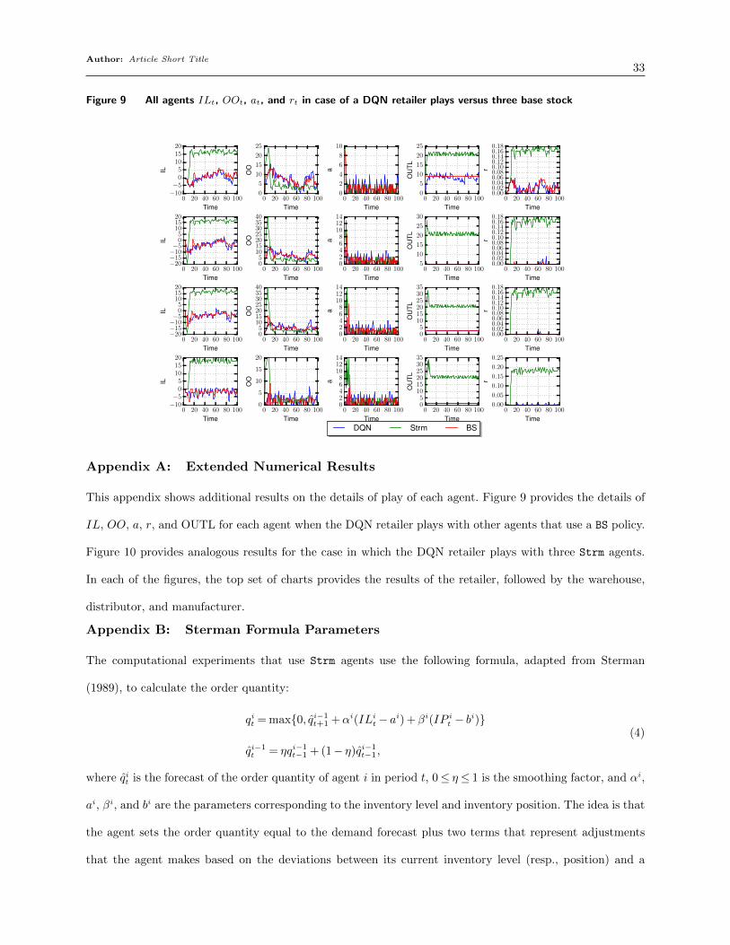
Figure 9 All agents ILt, OOt, at, and rt in case of a DQN retailer plays versus three base stock
0 20 40 60 80 100
Time
−10−5
05
101520
IL
0 20 40 60 80 100
Time
0
5
10
15
20
25
OO
0 20 40 60 80 100
Time
0
2
4
6
8
10
a
0 20 40 60 80 100
Time
0
5
10
15
20
25
OU
TL
0 20 40 60 80 100
Time
0.000.020.040.060.080.100.120.140.160.18
r
0 20 40 60 80 100
Time
−20−15−10−5
05
101520
IL
0 20 40 60 80 100
Time
05
10152025303540
OO
0 20 40 60 80 100
Time
02468
101214
a
0 20 40 60 80 100
Time
5
10
15
20
25
30
OU
TL
0 20 40 60 80 100
Time
0.000.020.040.060.080.100.120.140.160.18
r
0 20 40 60 80 100
Time
−20−15−10−5
05
101520
IL
0 20 40 60 80 100
Time
05
10152025303540
OO
0 20 40 60 80 100
Time
02468
101214
a0 20 40 60 80 100
Time
05
101520253035
OU
TL
0 20 40 60 80 100
Time
0.000.020.040.060.080.100.120.140.160.18
r
0 20 40 60 80 100
Time
−10−5
05
101520
IL
0 20 40 60 80 100
Time
0
5
10
15
20
OO
0 20 40 60 80 100
Time
02468
101214
a
0 20 40 60 80 100
Time
05
101520253035
OU
TL0 20 40 60 80 100
Time
0.00
0.05
0.10
0.15
0.20
0.25
r
DQN Strm BS
Appendix A: Extended Numerical Results
This appendix shows additional results on the details of play of each agent. Figure 9 provides the details of
IL, OO, a, r, and OUTL for each agent when the DQN retailer plays with other agents that use a BS policy.
Figure 10 provides analogous results for the case in which the DQN retailer plays with three Strm agents.
In each of the figures, the top set of charts provides the results of the retailer, followed by the warehouse,
distributor, and manufacturer.
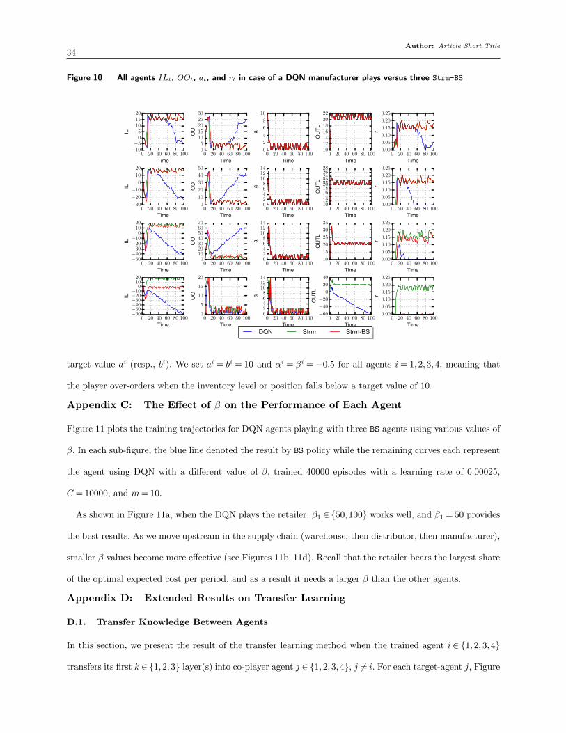
Appendix B: Sterman Formula Parameters
The computational experiments that use Strm agents use the following formula, adapted from Sterman
(1989), to calculate the order quantity:
qit = max{0, qi−1t+1 +αi(ILi
t− ai) +βi(IP it − bi)}
qi−1t = ηqi−1
t−1 + (1− η)qi−1t−1,
(4)
where qit is the forecast of the order quantity of agent i in period t, 0≤ η≤ 1 is the smoothing factor, and αi,
ai, βi, and bi are the parameters corresponding to the inventory level and inventory position. The idea is that
the agent sets the order quantity equal to the demand forecast plus two terms that represent adjustments
that the agent makes based on the deviations between its current inventory level (resp., position) and a
Author: Article Short Title34
Figure 10 All agents ILt, OOt, at, and rt in case of a DQN manufacturer plays versus three Strm-BS
0 20 40 60 80 100
Time
−10−5
05
101520
IL
0 20 40 60 80 100
Time
05
1015202530
OO
0 20 40 60 80 100
Time
0
2
4
6
8
10
a
0 20 40 60 80 100
Time
10121416182022
OU
TL
0 20 40 60 80 100
Time
0.00
0.05
0.10
0.15
0.20
0.25
r
0 20 40 60 80 100
Time
−30
−20
−10
0
10
20
IL
0 20 40 60 80 100
Time
0
10
20
30
40
50
OO
0 20 40 60 80 100
Time
02468
101214
a
0 20 40 60 80 100
Time
10121416182022242628
OU
TL
0 20 40 60 80 100
Time
0.00
0.05
0.10
0.15
0.20
0.25
r
0 20 40 60 80 100
Time
−50−40−30−20−10
01020
IL
0 20 40 60 80 100
Time
010203040506070
OO
0 20 40 60 80 100
Time
02468
101214
a0 20 40 60 80 100
Time
10
15
20
25
30
35
OU
TL
0 20 40 60 80 100
Time
0.00
0.05
0.10
0.15
0.20
0.25
r
0 20 40 60 80 100
Time
−60−50−40−30−20−10
01020
IL
0 20 40 60 80 100
Time
0
5
10
15
20
OO
0 20 40 60 80 100
Time
02468
101214
a
0 20 40 60 80 100
Time
−60
−40
−20
0
20
40
OU
TL0 20 40 60 80 100
Time
0.00
0.05
0.10
0.15
0.20
0.25
r
DQN Strm Strm-BS
target value ai (resp., bi). We set ai = bi = 10 and αi = βi =−0.5 for all agents i= 1,2,3,4, meaning that
the player over-orders when the inventory level or position falls below a target value of 10.
Appendix C: The Effect of β on the Performance of Each Agent
Figure 11 plots the training trajectories for DQN agents playing with three BS agents using various values of
β. In each sub-figure, the blue line denoted the result by BS policy while the remaining curves each represent
the agent using DQN with a different value of β, trained 40000 episodes with a learning rate of 0.00025,
C = 10000, and m= 10.
As shown in Figure 11a, when the DQN plays the retailer, β1 ∈ {50,100} works well, and β1 = 50 provides
the best results. As we move upstream in the supply chain (warehouse, then distributor, then manufacturer),
smaller β values become more effective (see Figures 11b–11d). Recall that the retailer bears the largest share
of the optimal expected cost per period, and as a result it needs a larger β than the other agents.
Appendix D: Extended Results on Transfer Learning
D.1. Transfer Knowledge Between Agents
In this section, we present the result of the transfer learning method when the trained agent i ∈ {1,2,3,4}
transfers its first k ∈ {1,2,3} layer(s) into co-player agent j ∈ {1,2,3,4}, j 6= i. For each target-agent j, Figure
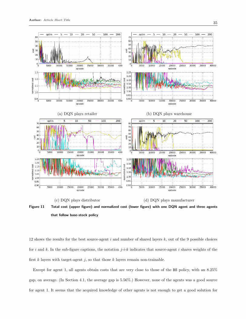
Author: Article Short Title35
(a) DQN plays retailer (b) DQN plays warehouse
(c) DQN plays distributor (d) DQN plays manufacturer
Figure 11 Total cost (upper figure) and normalized cost (lower figure) with one DQN agent and three agents
that follow base-stock policy
12 shows the results for the best source-agent i and number of shared layers k, out of the 9 possible choices
for i and k. In the sub-figure captions, the notation j-i-k indicates that source-agent i shares weights of the
first k layers with target-agent j, so that those k layers remain non-trainable.
Except for agent 1, all agents obtain costs that are very close to those of the BS policy, with an 8.25%
gap, on average. (In Section 4.1, the average gap is 5.56%.) However, none of the agents was a good source
for agent 1. It seems that the acquired knowledge of other agents is not enough to get a good solution for
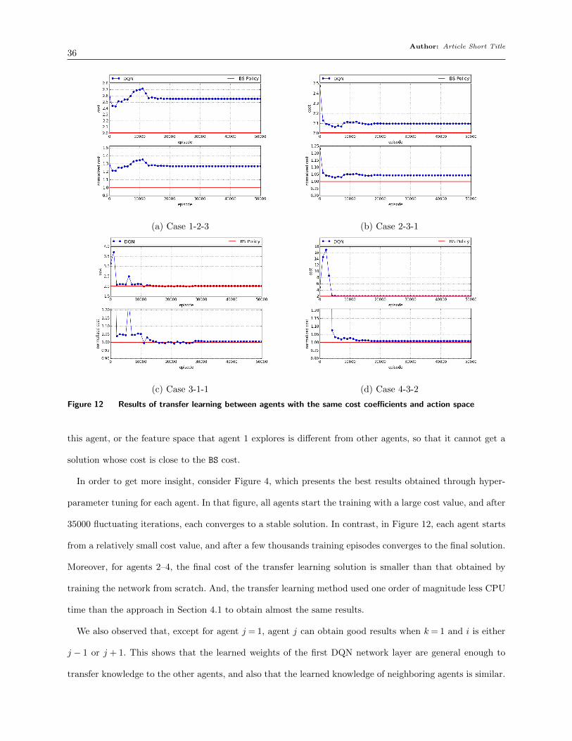
Author: Article Short Title36
(a) Case 1-2-3 (b) Case 2-3-1
(c) Case 3-1-1 (d) Case 4-3-2
Figure 12 Results of transfer learning between agents with the same cost coefficients and action space
this agent, or the feature space that agent 1 explores is different from other agents, so that it cannot get a
solution whose cost is close to the BS cost.
In order to get more insight, consider Figure 4, which presents the best results obtained through hyper-
parameter tuning for each agent. In that figure, all agents start the training with a large cost value, and after
35000 fluctuating iterations, each converges to a stable solution. In contrast, in Figure 12, each agent starts
from a relatively small cost value, and after a few thousands training episodes converges to the final solution.
Moreover, for agents 2–4, the final cost of the transfer learning solution is smaller than that obtained by
training the network from scratch. And, the transfer learning method used one order of magnitude less CPU
time than the approach in Section 4.1 to obtain almost the same results.
We also observed that, except for agent j = 1, agent j can obtain good results when k = 1 and i is either
j − 1 or j + 1. This shows that the learned weights of the first DQN network layer are general enough to
transfer knowledge to the other agents, and also that the learned knowledge of neighboring agents is similar.
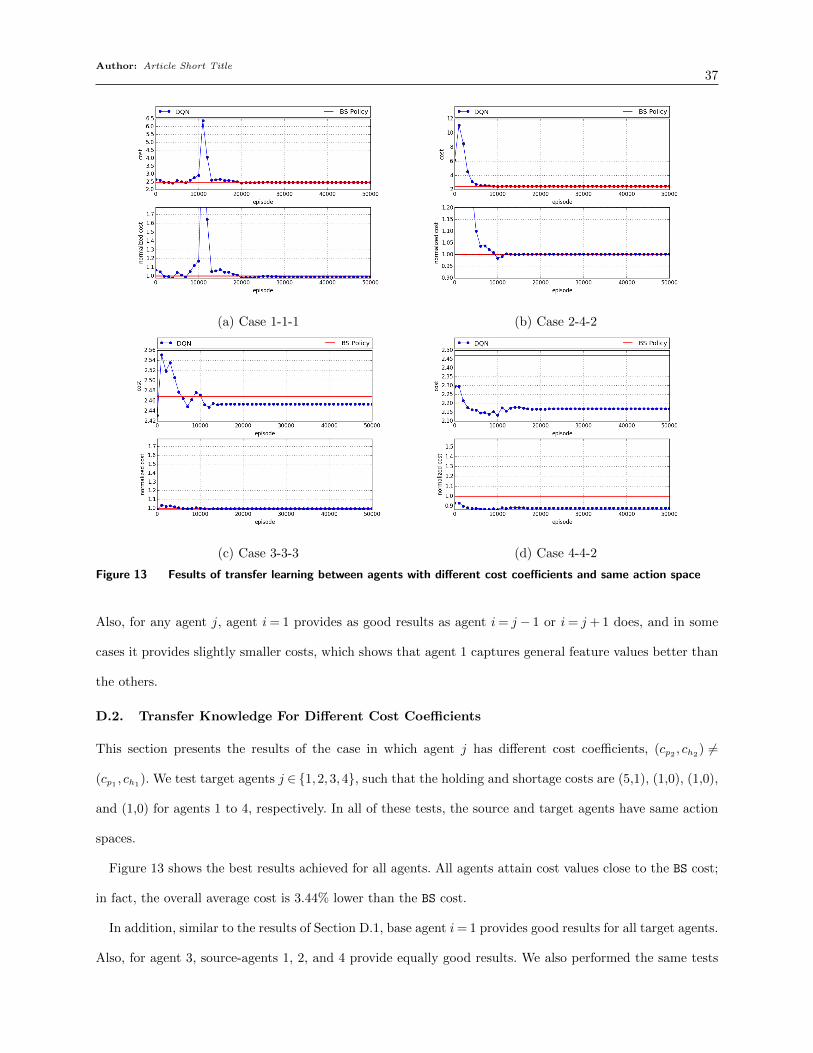
Author: Article Short Title37
(a) Case 1-1-1 (b) Case 2-4-2
(c) Case 3-3-3 (d) Case 4-4-2
Figure 13 Fesults of transfer learning between agents with different cost coefficients and same action space
Also, for any agent j, agent i= 1 provides as good results as agent i= j − 1 or i= j + 1 does, and in some
cases it provides slightly smaller costs, which shows that agent 1 captures general feature values better than
the others.
D.2. Transfer Knowledge For Different Cost Coefficients
This section presents the results of the case in which agent j has different cost coefficients, (cp2 , ch2) 6=
(cp1 , ch1). We test target agents j ∈ {1,2,3,4}, such that the holding and shortage costs are (5,1), (1,0), (1,0),
and (1,0) for agents 1 to 4, respectively. In all of these tests, the source and target agents have same action
spaces.
Figure 13 shows the best results achieved for all agents. All agents attain cost values close to the BS cost;
in fact, the overall average cost is 3.44% lower than the BS cost.
In addition, similar to the results of Section D.1, base agent i= 1 provides good results for all target agents.
Also, for agent 3, source-agents 1, 2, and 4 provide equally good results. We also performed the same tests

Author: Article Short Title38
(a) Case 1-1-2 (b) Case 2-2-1
(c) Case 3-3-1 (d) Case 4-4-1
Figure 14 Results of transfer learning between agents with same cost coefficients and different action spaces
with shortage and holding costs (10,1), (1,0), (1,0), and (1,0) for agents 1 to 4, respectively, and obtained
very similar results.
D.3. Transfer Knowledge For different Size of Action Space
Increasing the size of the action space should increase the accuracy of the d+x approach. However, it makes
the training process harder. It can be effective to train an agent with a small action space and then transfer
the knowledge to an agent with a larger action space. To test this, we test target-agent j ∈ {1,2,3,4} with
action space {−5, . . . ,5}, assuming that the source and target agents have the same cost coefficients.
Figure 14 shows the best results achieved for all agents. All agents attained costs that are close to the BS
cost, with an average gap of approximately 6.43%.