Embed Size (px)
Citation preview
A Defect Model of Reliability, IRPS ‘95 1 C. Glenn Shirley, Intel
A Defect Model of Reliability
C. Glenn ShirleyIntel Corp.
1995 International Reliability Physics Symposium
A Defect Model of Reliability, IRPS ‘95 2 C. Glenn Shirley, Intel
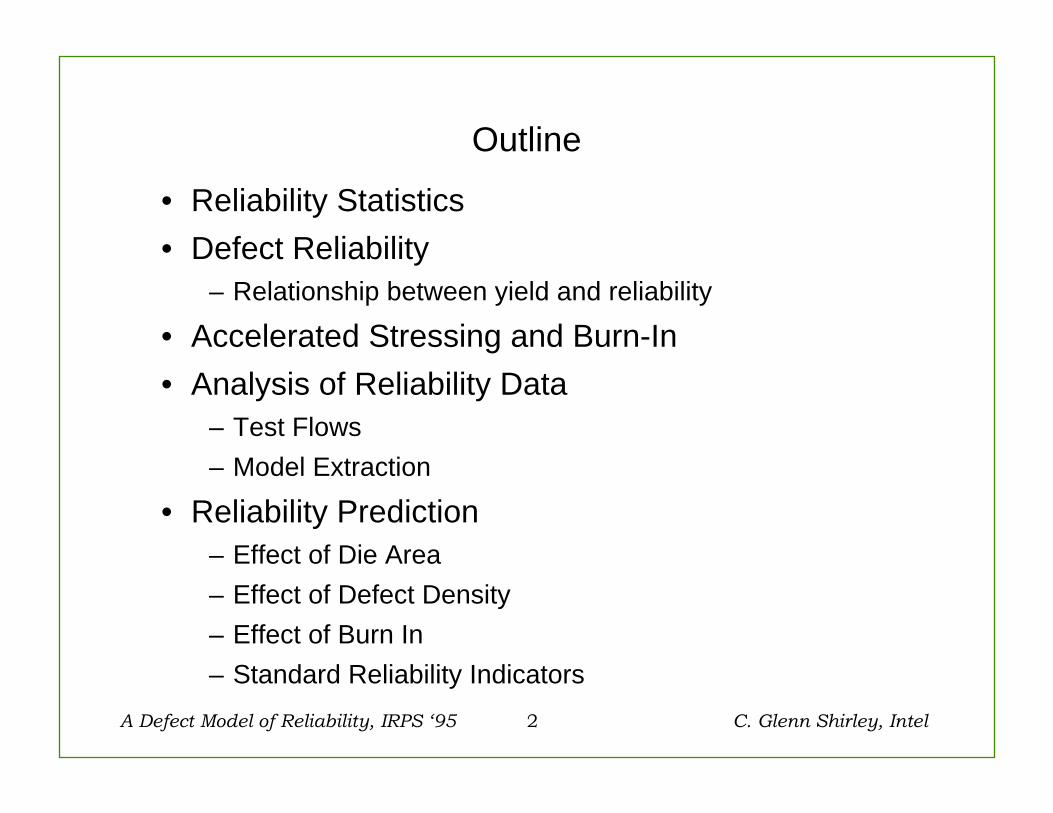
Outline
• Reliability Statistics• Defect Reliability
– Relationship between yield and reliability
• Accelerated Stressing and Burn-In• Analysis of Reliability Data
– Test Flows– Model Extraction
• Reliability Prediction– Effect of Die Area– Effect of Defect Density– Effect of Burn In– Standard Reliability Indicators
A Defect Model of Reliability, IRPS ‘95 3 C. Glenn Shirley, Intel
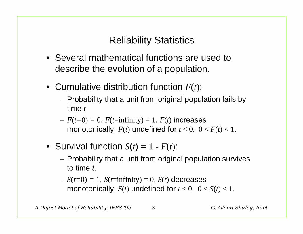
Reliability Statistics
• Several mathematical functions are used to describe the evolution of a population.
• Cumulative distribution function F(t):– Probability that a unit from original population fails by
time t– F(t=0) = 0, F(t=infinity) = 1, F(t) increases
monotonically, F(t) undefined for t < 0. 0 < F(t) < 1.
• Survival function S(t) = 1 - F(t):– Probability that a unit from original population survives
to time t.– S(t=0) = 1, S(t=infinity) = 0, S(t) decreases
monotonically, S(t) undefined for t < 0. 0 < S(t) < 1.
A Defect Model of Reliability, IRPS ‘95 4 C. Glenn Shirley, Intel
Reliability Statistics
0.1 0.2 0.4 1 2 4 10 200.00
0.10
0.20
0.30
0.40
0.50
0.60
0.70
0.80
0.901.00
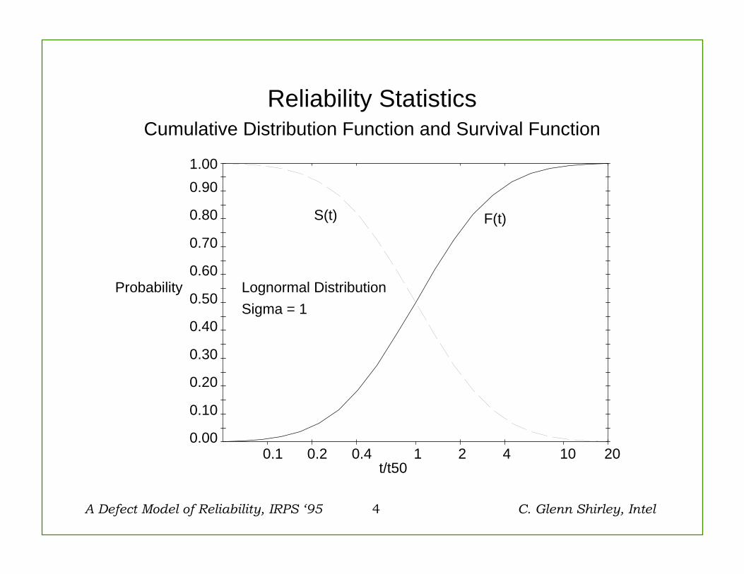
F(t)S(t)
t/t50
ProbabilitySigma = 1Lognormal Distribution
Cumulative Distribution Function and Survival Function

A Defect Model of Reliability, IRPS ‘95 5 C. Glenn Shirley, Intel
Reliability Statistics
• Probability density function, f(t)
– Of theoretical interest only.
f tdt
dt( ) = ×
Number of failures in Initial Population
1
f tdF t
dtdS t
dt( )
( ) ( )= = −
F t f t dtt
( ) ( )= ∫0
A Defect Model of Reliability, IRPS ‘95 6 C. Glenn Shirley, Intel
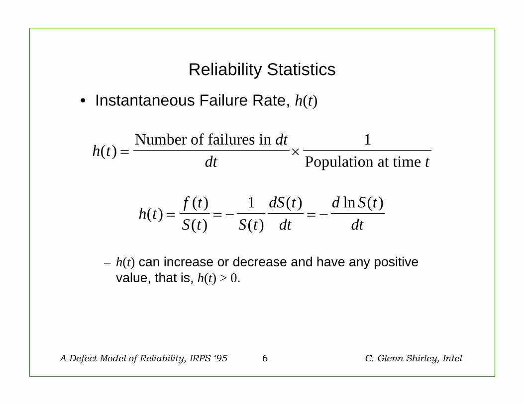
Reliability Statistics
• Instantaneous Failure Rate, h(t)
– h(t) can increase or decrease and have any positive value, that is, h(t) > 0.
h tdt
dt t( ) = ×
Number of failures in Population at time
1
h tf tS t S t
dS tdt
d S tdt
( )( )( ) ( )
( ) ln ( )= = − = −
1

A Defect Model of Reliability, IRPS ‘95 7 C. Glenn Shirley, Intel
Reliability Statistics
0.1 0.2 0.4 1 2 4 10 200.00
0.10
0.20
0.30
0.40
0.50
0.60
0.70
0.80
0.901.00
Time/t50
Failure Rate(1/sec)
f(t)
h(t)
Lognormal Distribution, sigma = 1
Probability Density Function f(t), and Instantaneous Failure Rate h(t)
A Defect Model of Reliability, IRPS ‘95 8 C. Glenn Shirley, Intel
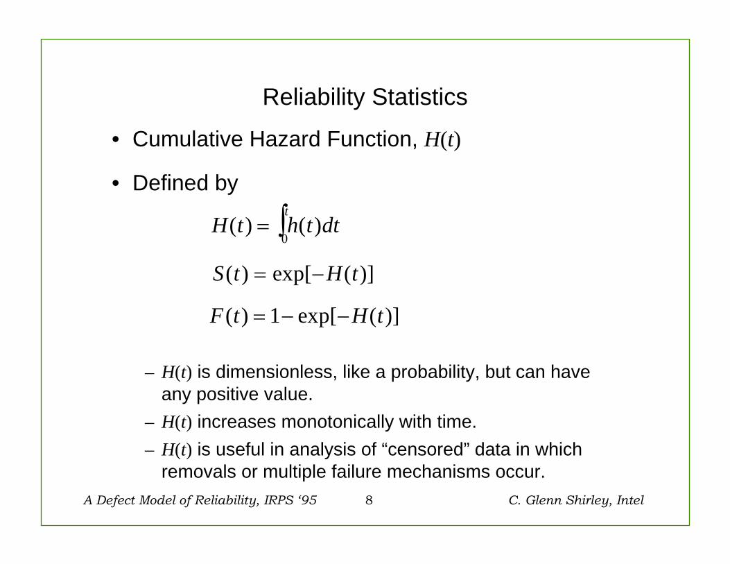
Reliability Statistics
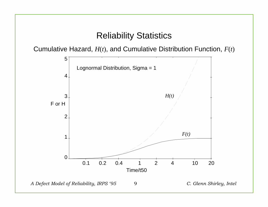
• Cumulative Hazard Function, H(t)
• Defined by
– H(t) is dimensionless, like a probability, but can have any positive value.
– H(t) increases monotonically with time.– H(t) is useful in analysis of “censored” data in which
removals or multiple failure mechanisms occur.
H t h t dtt
( ) ( )= ∫0
S t H t( ) exp[ ( )]= −
F t H t( ) exp[ ( )]= − −1
A Defect Model of Reliability, IRPS ‘95 9 C. Glenn Shirley, Intel
Reliability Statistics
0.1 0.2 0.4 1 2 4 10 200
1
2
3
4
5
F or H
Time/t50
H(t)
F(t)
Lognormal Distribution, Sigma = 1
Cumulative Hazard, H(t), and Cumulative Distribution Function, F(t)
A Defect Model of Reliability, IRPS ‘95 10 C. Glenn Shirley, Intel
Reliability Statistics
• The functions F(t), S(t), f(t), h(t), H(t) are all interrelated. Given one, the others can be derived.
• No assumptions about the specific distribution (Weibull, Lognormal, etc. have been made).
• A program for extracting models from censored data is
– Plot H(t) from censored data– Determine F(t) via F(t) = 1 - exp[-H(t)]– Fit parametric distribution to F(t)– Use parametric S(t) = 1 - F(t) to calculate predictions.
A Defect Model of Reliability, IRPS ‘95 11 C. Glenn Shirley, Intel
Reliability Statistics
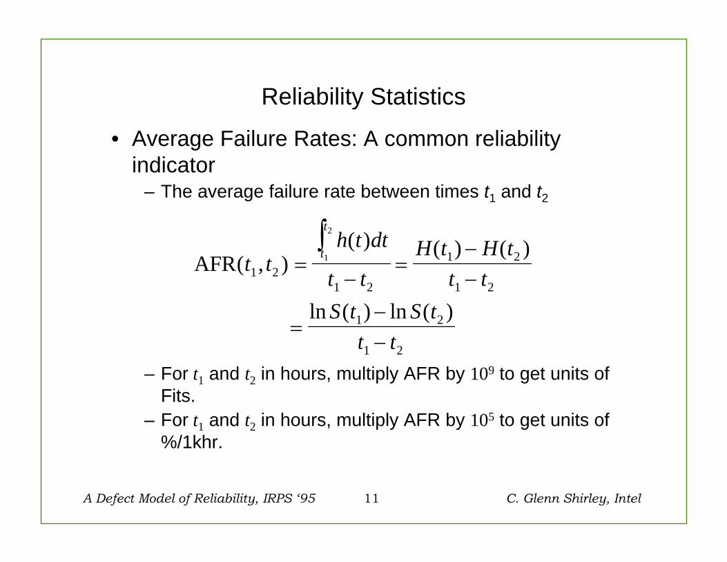
• Average Failure Rates: A common reliability indicator
– The average failure rate between times t1 and t2
– For t1 and t2 in hours, multiply AFR by 109 to get units of Fits.
– For t1 and t2 in hours, multiply AFR by 105 to get units of %/1khr.
AFR( , )( ) ( ) ( )
ln ( ) ln ( )
t th t dt
t tH t H t
t tS t S t
t t
t
t
1 21 2
1 2
1 2
1 2
1 2
1
2
=−
=−−
=−−
∫
A Defect Model of Reliability, IRPS ‘95 12 C. Glenn Shirley, Intel
Reliability Statistics
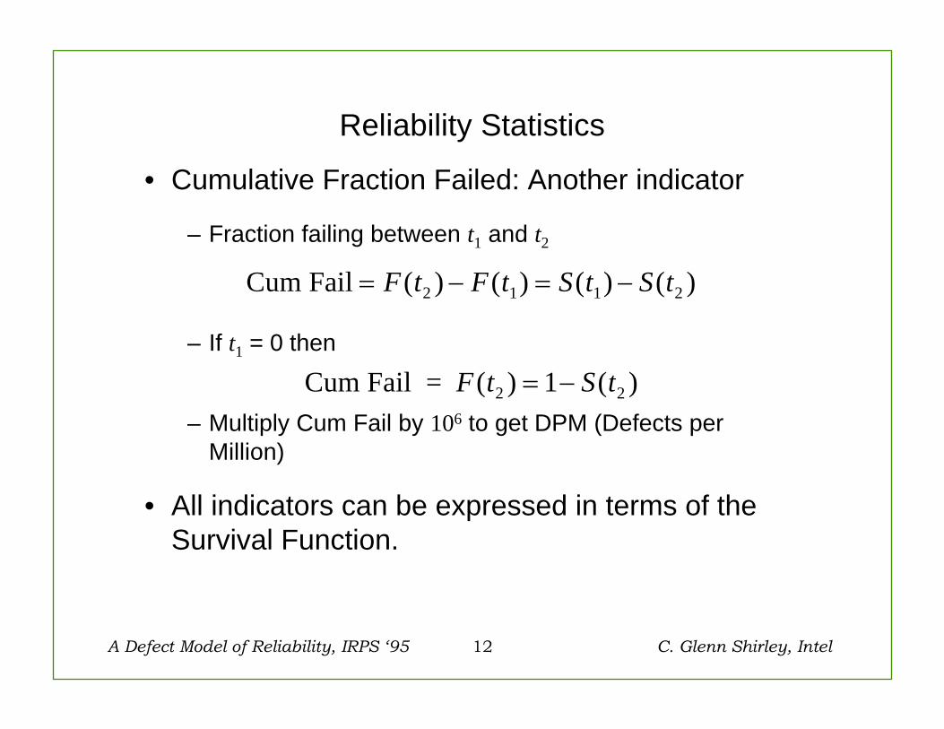
• Cumulative Fraction Failed: Another indicator
– Fraction failing between t1 and t2
– If t1 = 0 then
– Multiply Cum Fail by 106 to get DPM (Defects per Million)
• All indicators can be expressed in terms of the Survival Function.
Cum Fail = − = −F t F t S t S t( ) ( ) ( ) ( )2 1 1 2
Cum Fail = F t S t( ) ( )2 21= −

A Defect Model of Reliability, IRPS ‘95 13 C. Glenn Shirley, Intel
Reliability Statistics
• Multiple failure mechanisms– If the earliest occurrence of a mechanism is fatal, then
the device is logically a chain:
– This is the usual case for semiconductor components. That is, there is no functional redundancy.
DefectMechanism
1
DefectMechanism
2
DefectMechanism
3
IntrinsicMechanism
1
IntrinsicMechanism
2
IntrinsicMechanism
3
Etc.
A Defect Model of Reliability, IRPS ‘95 14 C. Glenn Shirley, Intel
Reliability Statistics
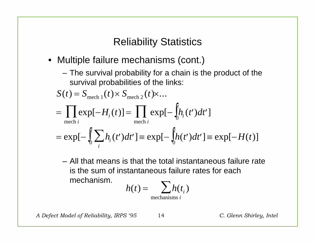
• Multiple failure mechanisms (cont.)– The survival probability for a chain is the product of the
survival probabilities of the links:
– All that means is that the total instantaneous failure rate is the sum of instantaneous failure rates for each mechanism.
S t S t S t
H t h t dt
h t dt h t dt H t
ii
i
t
i
ii
tt
( ) ( ) ( ) ...
exp[ ( )] exp[ ( ) ]
exp[ ( ) ] exp[ ( ) ] exp[ ( )]
= × ×
= − = − ′ ′
= − ′ ′ ≡ − ′ ′ ≡ −
∏ ∫∏
∑ ∫∫
mech 1 mech 2
mech mech 0
00
h t h tii
( ) ( )= ∑mechanisms

A Defect Model of Reliability, IRPS ‘95 15 C. Glenn Shirley, Intel
Intrinsic versus Defect Mechanisms
• Intrinsic mechanisms are due to non-defect-related manufacturing or design errors.
– Typically associated with gross areas of the wafer.
• The total survival function may be written
• The focus in this tutorial is on defect-related mechanisms.
– These are the main concern in the manufacturing environment.
S t S t S t
S t S t
( ) ( ) ( ) ...
( ) ( ) ...
= × ×
× × ×intrinsic mech 1 intrinsic mech 2
defect mech 1 defect mech 2

A Defect Model of Reliability, IRPS ‘95 16 C. Glenn Shirley, Intel
Defect Reliability• Factory production reliability issues are dominated by
defects.
• The same kinds of defects that degrade yield, degrade reliability.
– Yield is measured before any stress: At “Sort” (wafer-level functional test) and pre-burn-in class test.
– Reliability is measured by post-burn-in class test.
• Since the “yield” and “reliability” defects are from the same source, yield and defect reliability are related.
• Yield is routinely measured - it can be used to predict reliability.
• Yield fallout is easier to measure than reliability fallout: It is larger.
A Defect Model of Reliability, IRPS ‘95 17 C. Glenn Shirley, Intel
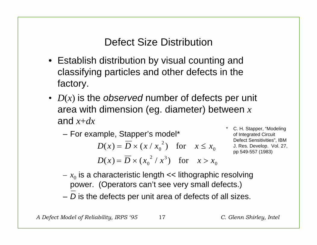
Defect Size Distribution
• Establish distribution by visual counting and classifying particles and other defects in the factory.
• D(x) is the observed number of defects per unit area with dimension (eg. diameter) between xand x+dx
– For example, Stapper’s model*
– x0 is a characteristic length << lithographic resolving power. (Operators can’t see very small defects.)
– D is the defects per unit area of defects of all sizes.
D x D x x x x( ) ( / )= × ≤02
0for
D x D x x x x( ) ( / )= × >02 3
0for
* C. H. Stapper, “Modeling of Integrated Circuit Defect Sensitivities”, IBMJ. Res. Develop. Vol. 27, pp 549-557 (1983)
A Defect Model of Reliability, IRPS ‘95 18 C. Glenn Shirley, Intel
Probability of “Yield” and “Reliability” Defects.
• “Yield” defects prevent operation of the device at before any stress (t = 0).
• Latent “reliability” defects will eventually kill the device (that is, at t > 0).
• In simple cases, the probability of occurrence of a given defect type can be calculated as a function of defect size, assuming random spatial distribution of defects.*
• We’ll calculate the probability of “Yield” defects and “Reliability plus Yield” defects falling on a metal comb.
* See, for example, C. H. Stapper, “Modeling of defects in integrated circuit photolithographic patterns.” IBM J. Res. Develop. Vol. 28, pp 461-475 (1984)
A Defect Model of Reliability, IRPS ‘95 19 C. Glenn Shirley, Intel
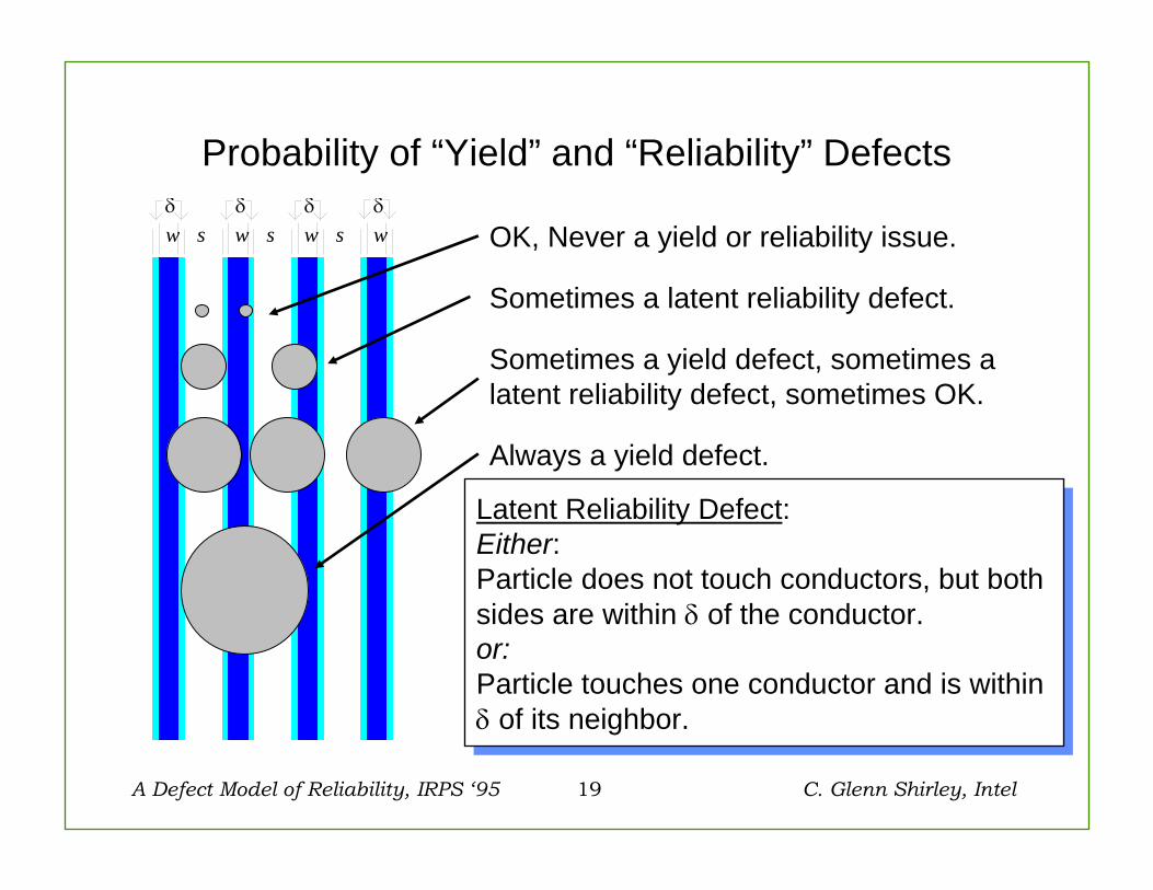
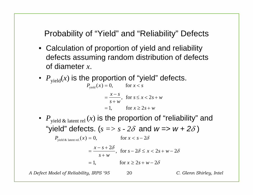
Probability of “Yield” and “Reliability” Defects
s s swww wδδδ δ
Latent Reliability Defect:Either:Particle does not touch conductors, but both sides are within δ of the conductor.or:Particle touches one conductor and is within δ of its neighbor.
Latent Reliability Defect:Either:Particle does not touch conductors, but both sides are within δ of the conductor.or:Particle touches one conductor and is within δ of its neighbor.
OK, Never a yield or reliability issue.
Sometimes a latent reliability defect.
Sometimes a yield defect, sometimes alatent reliability defect, sometimes OK.
Always a yield defect.
A Defect Model of Reliability, IRPS ‘95 20 C. Glenn Shirley, Intel
Probability of “Yield” and “Reliability” Defects
• Calculation of proportion of yield and reliability defects assuming random distribution of defects of diameter x.
• Pyield(x) is the proportion of “yield” defects.
• Pyield & latent rel (x) is the proportion of “reliability” and “yield” defects. (s => s - 2δ and w => w + 2δ )
P x x s
x ss w
s x s w
x s w
yield & latent rel. for
, for
, for
( ) ,= < −
=− +
+− ≤ < + −
= ≥ + −
0 2
2 2 2 2
1 2 2
δ
δδ δ
δ
P x x sx ss w
s x s w
x s w
yield for
, for
, for
( ) ,= <
=−+
≤ < +
= ≥ +
0
2
1 2

A Defect Model of Reliability, IRPS ‘95 21 C. Glenn Shirley, Intel
Yield and Reliability Defect Densities
• Combine– Defect size distribution.– Probability of type of defect vs defect size.
• Calculate the defect density of defects– which are fatal to device at t = 0:
– and those which are latent reliability defects:
D D x P x dx Dxs w syield yield= =
+
∞
∫ ( ) ( )( )0
0
2 2
D D x P x dxDx
s w s s w srelrel = =− + −
−+
⎡⎣⎢
⎤⎦⎥
∞∫ ( ) ( )( )( ) ( )
00 2
12 2 2
12δ δ

A Defect Model of Reliability, IRPS ‘95 22 C. Glenn Shirley, Intel
Yield and Reliability Defect Densities
Defect SizeDistribution
Proportion ofDefects P(x)
Shorting lines: Pyield(x)
Proportion ofLatent Rel. DefectsPrel(x) x0
Latent or shorting lines:Prel(x) + Pyield(x)
ss-2δ 2s+w2s+w-2δ
Defect Size
D x Dx x( ) /= 02 3
A Defect Model of Reliability, IRPS ‘95 23 C. Glenn Shirley, Intel
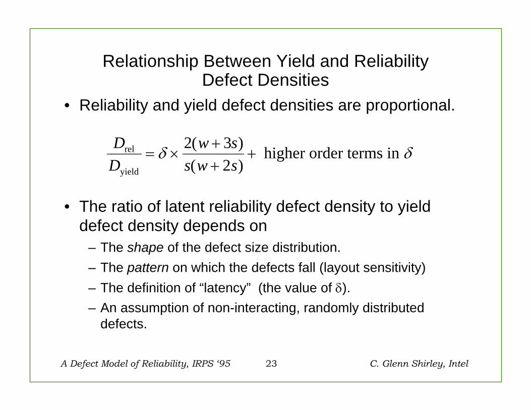
Relationship Between Yield and Reliability Defect Densities
• Reliability and yield defect densities are proportional.
• The ratio of latent reliability defect density to yield defect density depends on
– The shape of the defect size distribution.– The pattern on which the defects fall (layout sensitivity)– The definition of “latency” (the value of δ).– An assumption of non-interacting, randomly distributed
defects.
DD
w ss w s
rel
yield
higher order terms in = ×++
+δ δ2 32
( )( )
A Defect Model of Reliability, IRPS ‘95 24 C. Glenn Shirley, Intel
Relationship Between Yield and Reliability Defect Densities
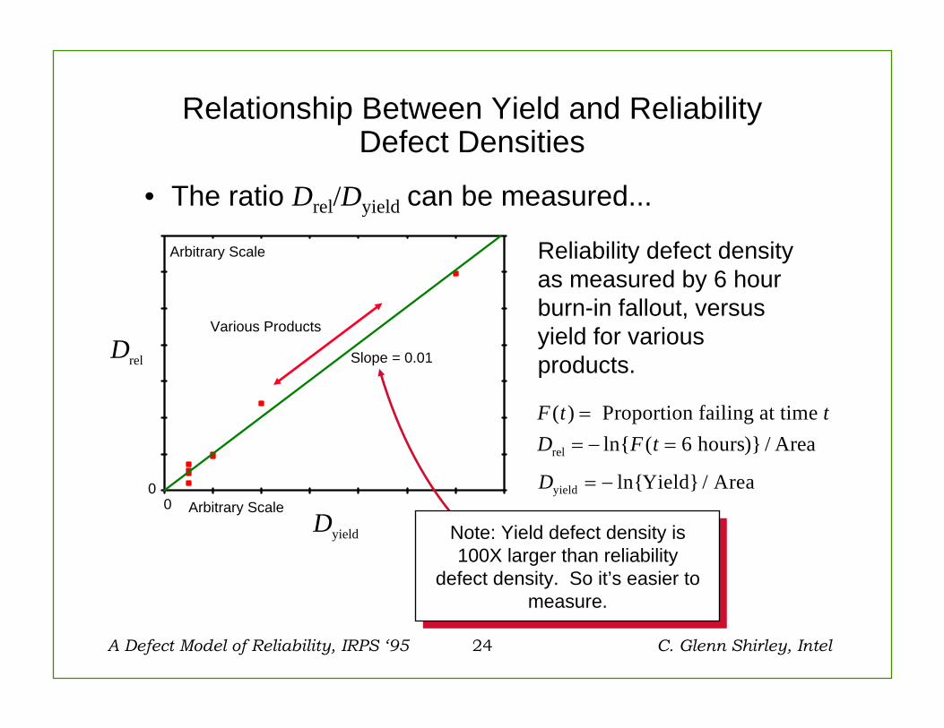
• The ratio Drel/Dyield can be measured...
Reliability defect density as measured by 6 hour burn-in fallout, versus yield for various products.
F t tD F t
( )ln{ ( )} /
== − =
Proportion failing at time hours Arearel 6
Dyield Yield Area= − ln{ } /
Drel
Dyield
Arbitrary Scale0
0
Arbitrary Scale
Slope = 0.01
Various Products
Note: Yield defect density is 100X larger than reliability
defect density. So it’s easier to measure.
Note: Yield defect density is 100X larger than reliability
defect density. So it’s easier to measure.

A Defect Model of Reliability, IRPS ‘95 25 C. Glenn Shirley, Intel
Simulation of Defect Reliability
• In general, analytical calculation of reliability and yield defectivities is complex because of
– Complex defect size distributions.
– Non-circular defects with orientation distributions.
– Complex substrate patterns.
• Often it is easier to use Monte Carlo methods to evaluate defectivities by simulation.
• We’ll discuss simulation more when we look at an assembly-related example a bit later.
A Defect Model of Reliability, IRPS ‘95 26 C. Glenn Shirley, Intel
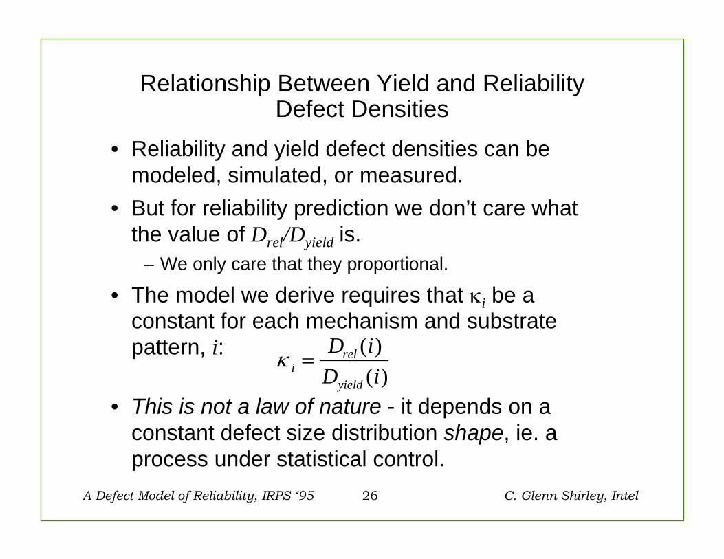
Relationship Between Yield and Reliability Defect Densities
• Reliability and yield defect densities can be modeled, simulated, or measured.
• But for reliability prediction we don’t care what the value of Drel/Dyield is.
– We only care that they proportional.
• The model we derive requires that κi be a constant for each mechanism and substrate pattern, i:
• This is not a law of nature - it depends on a constant defect size distribution shape, ie. a process under statistical control.
κ irel
yield
D iD i
=( )( )
A Defect Model of Reliability, IRPS ‘95 27 C. Glenn Shirley, Intel
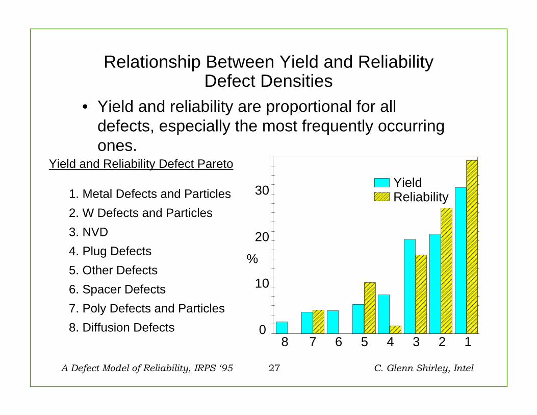
Relationship Between Yield and Reliability Defect Densities
• Yield and reliability are proportional for all defects, especially the most frequently occurring ones.
0
10
20
30
%
YieldReliability
12345678
1. Metal Defects and Particles2. W Defects and Particles3. NVD4. Plug Defects5. Other Defects6. Spacer Defects7. Poly Defects and Particles8. Diffusion Defects
Yield and Reliability Defect Pareto
A Defect Model of Reliability, IRPS ‘95 28 C. Glenn Shirley, Intel
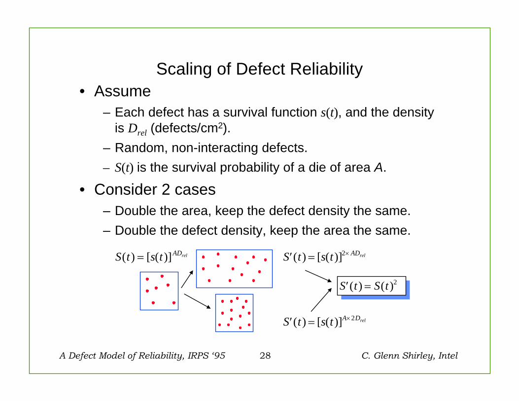
Scaling of Defect Reliability
S t s t ADrel( ) [ ( )]= ′ = ×S t s t ADrel( ) [ ( )]2
′ = ×S t s t A Drel( ) [ ( )] 2
′ =S t S t( ) ( )2
• Assume– Each defect has a survival function s(t), and the density
is Drel (defects/cm2).– Random, non-interacting defects.– S(t) is the survival probability of a die of area A.
• Consider 2 cases– Double the area, keep the defect density the same.– Double the defect density, keep the area the same.
A Defect Model of Reliability, IRPS ‘95 29 C. Glenn Shirley, Intel
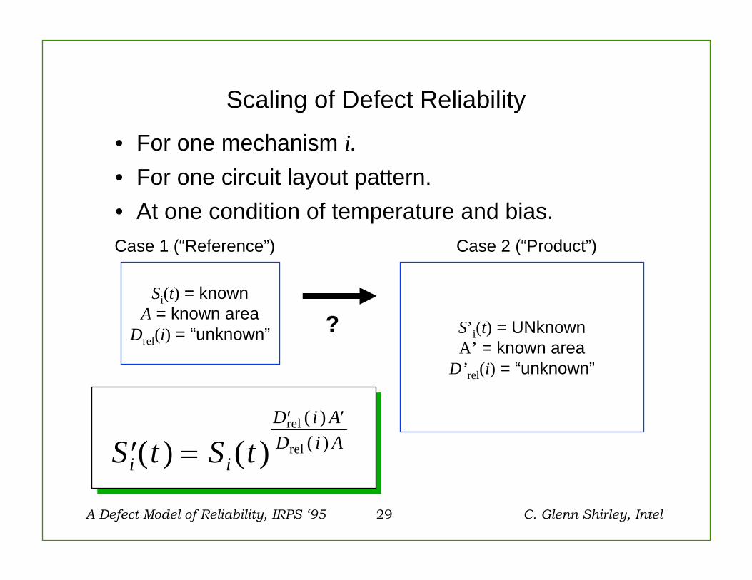
Scaling of Defect Reliability
• For one mechanism i.• For one circuit layout pattern.• At one condition of temperature and bias.
Si(t) = knownA = known area
Drel(i) = “unknown” S’i(t) = UNknownA’ = known area
D’rel(i) = “unknown”
?
Case 1 (“Reference”) Case 2 (“Product”)
′ =′ ′
S t S ti i
D i AD i A( ) ( )
( )( )
rel
rel
A Defect Model of Reliability, IRPS ‘95 30 C. Glenn Shirley, Intel
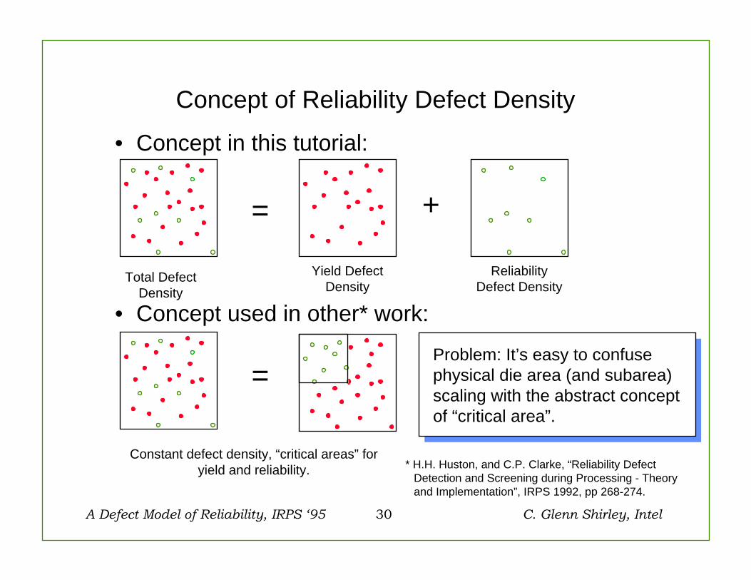
Concept of Reliability Defect Density
• Concept in this tutorial:
• Concept used in other* work:
= +
Total DefectDensity
Yield DefectDensity
ReliabilityDefect Density
=
Constant defect density, “critical areas” for yield and reliability. * H.H. Huston, and C.P. Clarke, “Reliability Defect
Detection and Screening during Processing - Theory and Implementation”, IRPS 1992, pp 268-274.
Problem: It’s easy to confuse physical die area (and subarea) scaling with the abstract concept of “critical area”.
Problem: It’s easy to confuse physical die area (and subarea) scaling with the abstract concept of “critical area”.
A Defect Model of Reliability, IRPS ‘95 31 C. Glenn Shirley, Intel
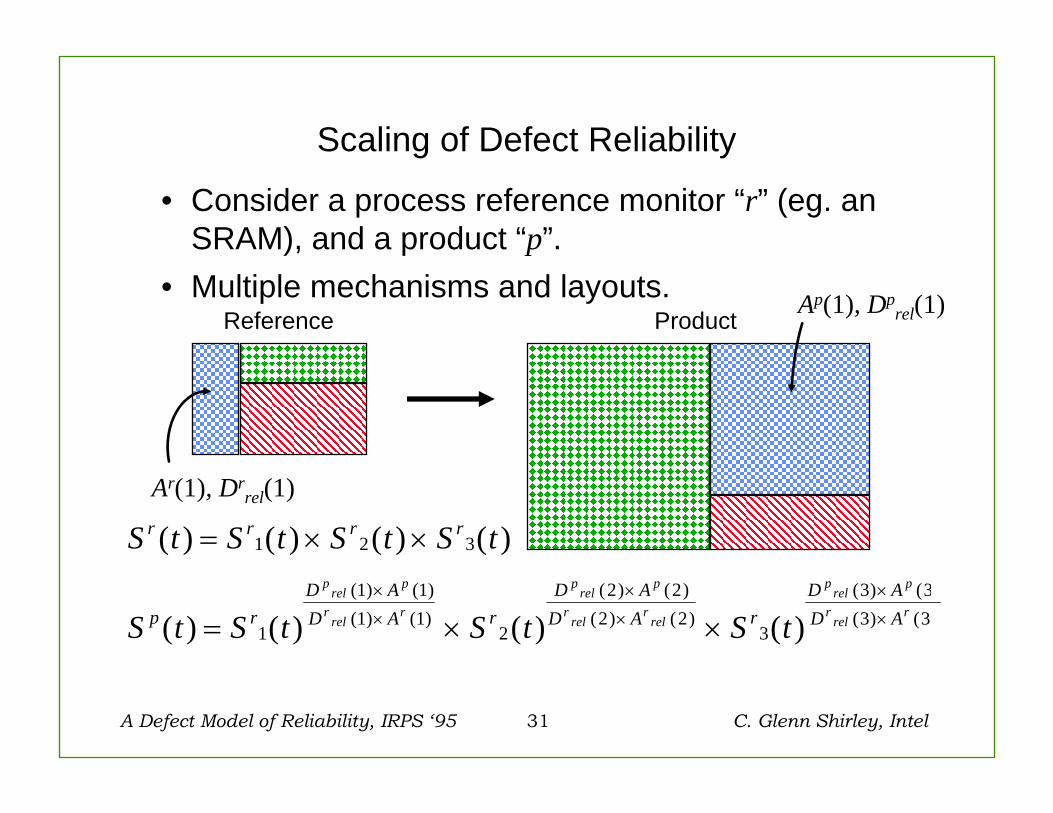
Scaling of Defect Reliability
• Consider a process reference monitor “r” (eg. an SRAM), and a product “p”.
• Multiple mechanisms and layouts.Reference Product
S t S t S t S t
S t S t S t S t
r r r r
p rD AD A r
D AD A r
D AD A
prel
p
rrel
r
prel
p
rrel
rrel
prel
p
rrel
r
( ) ( ) ( ) ( )
( ) ( ) ( ) ( )(1) (1)(1) (1)
( ) ( )( ) ( )
( ) (( ) (
= × ×
= × ××
×
×
×
×
×
1 2 3
1 2
2 22 2
3
3 33 3
Ar(1), Drrel(1)
Ap(1), Dprel(1)
A Defect Model of Reliability, IRPS ‘95 32 C. Glenn Shirley, Intel
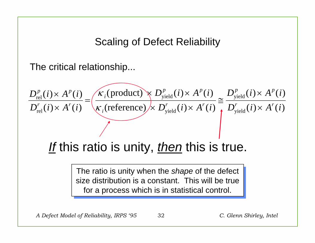
Scaling of Defect Reliability
D i A iD i A i
D i A iD i A i
D i A iD i A i
p p
r ri
p p
ir r
p p
r rrel
rel
yield
yield
yield
yield
product)(reference)
( ) ( )( ) ( )
( ( ) ( )( ) ( )
( ) ( )( ) ( )
××
=× ×
× ×≅
×
×
κκ
If this ratio is unity, then this is true.
The ratio is unity when the shape of the defect size distribution is a constant. This will be true
for a process which is in statistical control.
The ratio is unity when the shape of the defect size distribution is a constant. This will be true
for a process which is in statistical control.
The critical relationship...
A Defect Model of Reliability, IRPS ‘95 33 C. Glenn Shirley, Intel
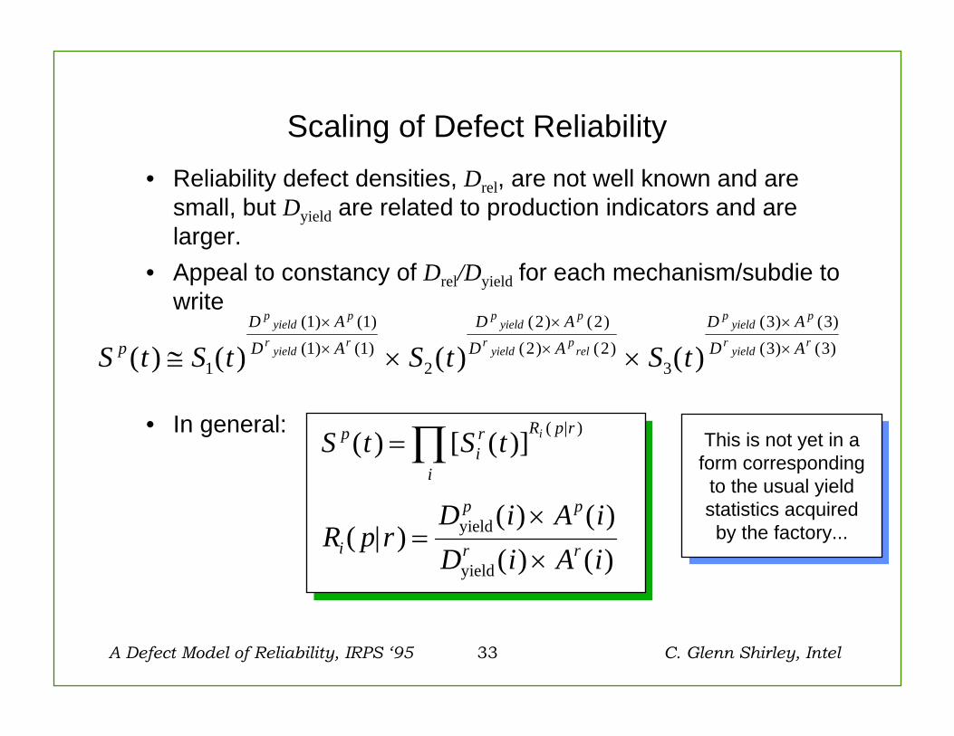
• Reliability defect densities, Drel, are not well known and are small, but Dyield are related to production indicators and are larger.
• Appeal to constancy of Drel/Dyield for each mechanism/subdie to write
• In general:
S t S t S t S tpD AD A
D AD A
D AD A
pyield
p
ryield
r
pyield
p
ryield
prel
pyield
p
ryield
r
( ) ( ) ( ) ( )(1) (1)(1) (1)
( ) ( )( ) ( )
( ) ( )( ) ( )≅ × ×
×
×
×
×
×
×1 2
2 22 2
3
3 33 3
Scaling of Defect Reliability
This is not yet in a form corresponding
to the usual yield statistics acquired by the factory...
This is not yet in a form corresponding
to the usual yield statistics acquired by the factory...
S t S t
R p rD i A iD i A i
pir
i
R p r
i
p p
r r
i( ) [ ( )]
( | )( ) ( )( ) ( )
( | )=
=×
×
∏
yield
yield

A Defect Model of Reliability, IRPS ‘95 34 C. Glenn Shirley, Intel
Y Y D A D A
D A
Y Y D j A j Y D A
D A YY
DD j A j
AA A j
p p p p p p
p p
p p p p
j
p p p
p pp
p
p
p p
ip
p p
j
= × − × −
× −
= × −⎛
⎝⎜
⎞
⎠⎟ = × − ×
× = −⎛⎝⎜
⎞⎠⎟
≡ ≡
∑
∑∑
intrinsic yield yield
yield
intrinsic yield intrinsic yield
yieldintrinsic
yield
exp[ ( ) ( )] exp[ ( ) ( )]
exp[ ( ) ( )]
exp ( ) ( ) exp( )
ln
( ) ( )( )
1 1 2 2
3 3
Yield Statistics
• Assuming Poisson statistics, the yield for the compound die is given by
Subdie area-weighteddefect density.
Total die area.
A Defect Model of Reliability, IRPS ‘95 35 C. Glenn Shirley, Intel
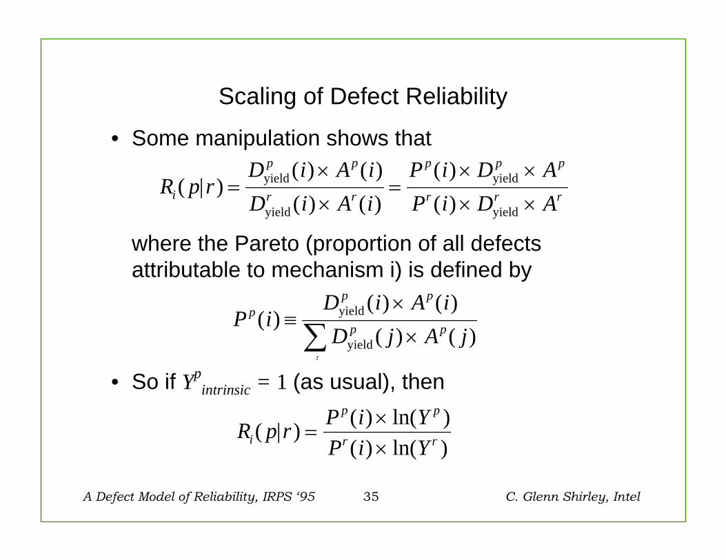
Scaling of Defect Reliability
• Some manipulation shows that
where the Pareto (proportion of all defects attributable to mechanism i) is defined by
• So if Ypintrinsic = 1 (as usual), then
R p rD i A iD i A i
P i D AP i D Ai
p p
r r
p p p
r r r( | )( ) ( )( ) ( )
( )( )
=×
×=
× ×
× ×yield
yield
yield
yield
P iD i A iD j A j
pp p
p p
j
( )( ) ( )( ) ( )
≡×
×∑yield
yield
R p r P i YP i Yi
p p
r r( | ) ( ) ln( )( ) ln( )
=××
A Defect Model of Reliability, IRPS ‘95 36 C. Glenn Shirley, Intel
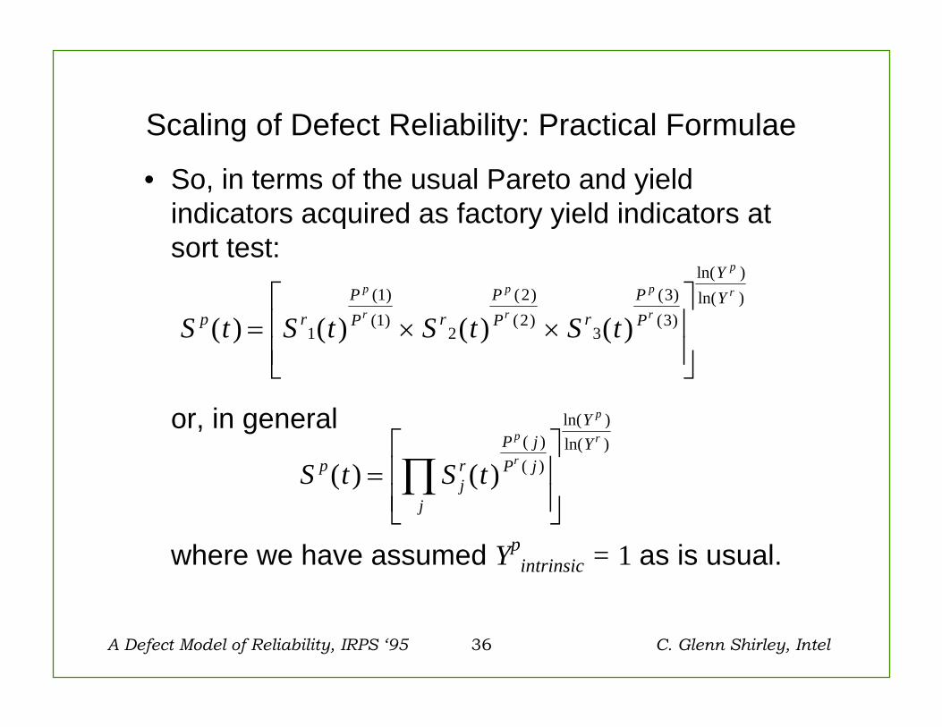
Scaling of Defect Reliability: Practical Formulae
• So, in terms of the usual Pareto and yield indicators acquired as factory yield indicators at sort test:
or, in general
where we have assumed Ypintrinsic = 1 as is usual.
S t S t S t S tp rPP r
PP r
PP
YYp
r
p
r
p
r
p
r
( ) ( ) ( ) ( )(1)(1)
( )( )
( )( )
ln( )ln( )
= × ×⎡
⎣⎢⎢
⎤
⎦⎥⎥
1 2
22
3
33
S t S tpjr
P jP j
j
YYp
r
p
r
( ) ( )( )( )
ln( )ln( )
=⎡
⎣⎢⎢
⎤
⎦⎥⎥
∏
A Defect Model of Reliability, IRPS ‘95 37 C. Glenn Shirley, Intel
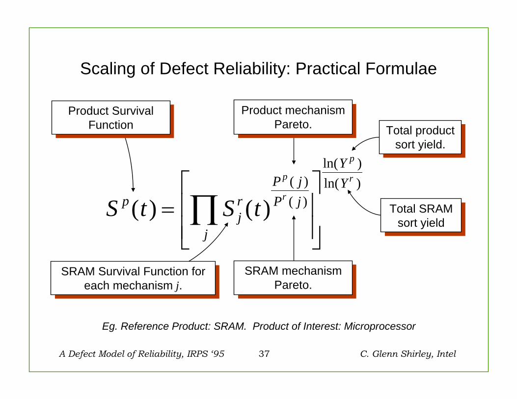
Scaling of Defect Reliability: Practical Formulae
S t S tpjr
P jP j
j
YYp
r
p
r
( ) ( )( )( )
ln( )ln( )
=⎡
⎣⎢⎢
⎤
⎦⎥⎥
∏ Total SRAMsort yield
Total SRAMsort yield
Eg. Reference Product: SRAM. Product of Interest: Microprocessor
SRAM mechanismPareto.
SRAM mechanismPareto.
Product mechanismPareto.
Product mechanismPareto.
Total product sort yield.
Total product sort yield.
Product Survival Function
Product Survival Function
SRAM Survival Function foreach mechanism j.
SRAM Survival Function foreach mechanism j.

A Defect Model of Reliability, IRPS ‘95 38 C. Glenn Shirley, Intel
• If the defect paretos are the same for reference and “unknown” product, then
so
where the total reference (usually SRAM) survival function is
Scaling of Defect Reliability: Practical Formulae
Usually a good approximation
since only one or two mechanisms
dominate.
Usually a good approximation
since only one or two mechanisms
dominate.
P i P i ip r( ) ( )= , for each
S t S tp rYY
p
r( ) ( )
ln( )ln( )=
S t S trjr
j
( ) ( )= ∏
A Defect Model of Reliability, IRPS ‘95 39 C. Glenn Shirley, Intel
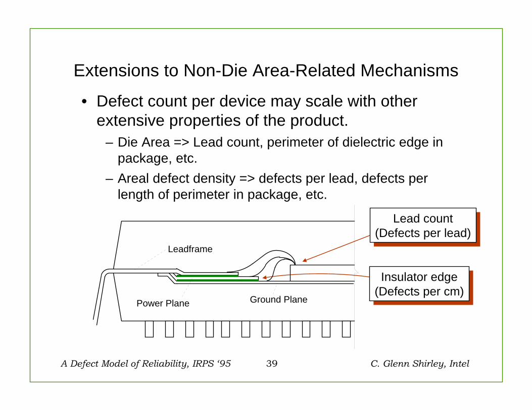
Extensions to Non-Die Area-Related Mechanisms
• Defect count per device may scale with other extensive properties of the product.
– Die Area => Lead count, perimeter of dielectric edge in package, etc.
– Areal defect density => defects per lead, defects per length of perimeter in package, etc.
Leadframe
Power Plane Ground Plane
Lead count(Defects per lead)
Lead count(Defects per lead)
Insulator edge(Defects per cm)Insulator edge
(Defects per cm)
A Defect Model of Reliability, IRPS ‘95 40 C. Glenn Shirley, Intel
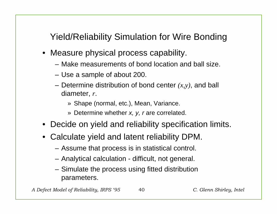
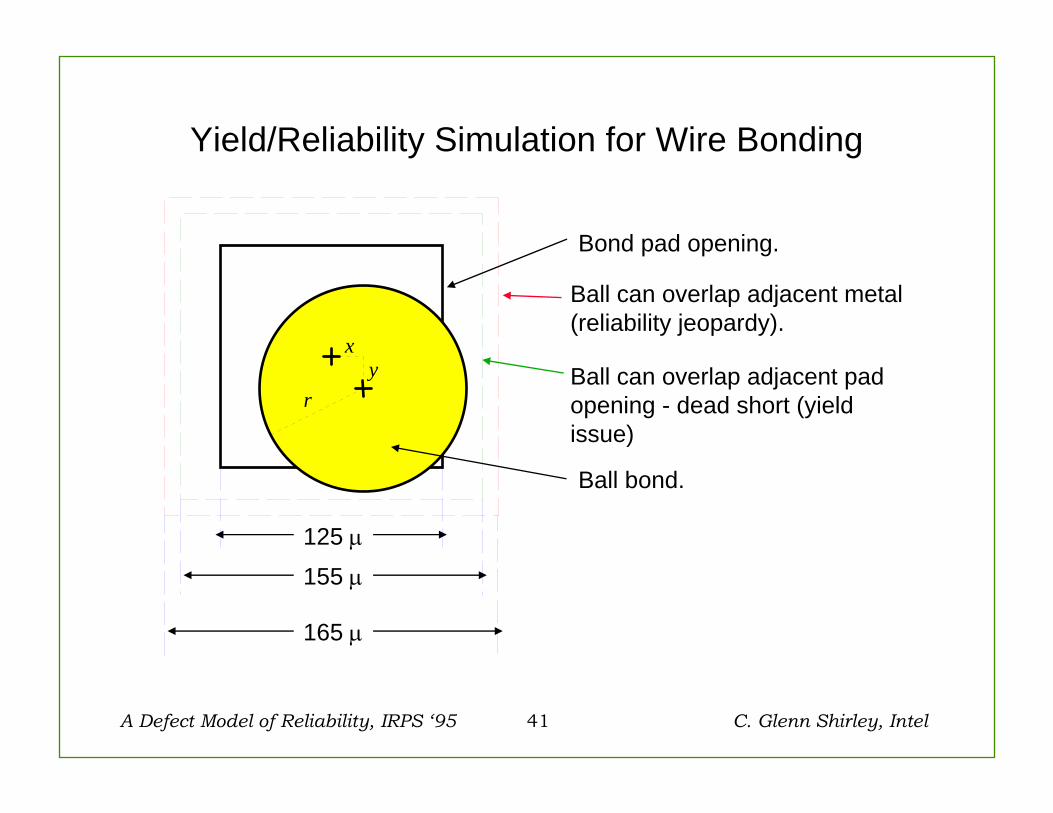
Yield/Reliability Simulation for Wire Bonding
• Measure physical process capability.– Make measurements of bond location and ball size.– Use a sample of about 200.– Determine distribution of bond center (x,y), and ball
diameter, r.» Shape (normal, etc.), Mean, Variance.» Determine whether x, y, r are correlated.
• Decide on yield and reliability specification limits.• Calculate yield and latent reliability DPM.
– Assume that process is in statistical control.– Analytical calculation - difficult, not general.– Simulate the process using fitted distribution
parameters.
A Defect Model of Reliability, IRPS ‘95 41 C. Glenn Shirley, Intel
Yield/Reliability Simulation for Wire Bonding
xy
r
Bond pad opening.
Ball bond.
Ball can overlap adjacent metal (reliability jeopardy).
Ball can overlap adjacent pad opening - dead short (yield issue)
165 μ
125 μ
155 μ

A Defect Model of Reliability, IRPS ‘95 42 C. Glenn Shirley, Intel
Yield/Reliability Simulation for Wire Bonding
-15 -10 -5 0 5 10 15 0.01
0.1
1
10 20 30 40 50 60 70 80 90
99
99.9
99.99
X: Mean = -0.89, SD = 4.34
Y: Mean = -2.17, SD = 6.75
Cum %
Distance from Center of Pad (microns)
40 42 44 46 48 50 52 54 56 58 60 0.01
0.1
1
10 20 30 40 50 60 70 80 90
99
99.9
99.99
Ideal Process: Mean = 49.32, SD = 2.25
Actual: Mean = 49.73, SD = 3.17
Cum %
Ball Radius (microns)
-20 -15 -10 -5 0 5 10 15 20 -20
-15
-10
-5
0
5
10
15
20
X-Position (microns)
Y-Position (microns)
(x,y) Distributionsr Distribution
• x, y, and r distributions are normal and uncorrelated.
• The parameters of the process in “statistical control” are
• x, y, and r distributions are normal and uncorrelated.
• The parameters of the process in “statistical control” are
x Mean x SD y Mean y SD r Mean r SD0 4.34 0 6.75 49.3 2.25
Outliers

A Defect Model of Reliability, IRPS ‘95 43 C. Glenn Shirley, Intel
Yield/Reliability Simulation for Wire Bonding
r
x
y
d
d
d/2
• Individual bonds are points clustering around the target.
• Bonds inside pyramid pass the criterion.
• Bonds outside the pyramid fail the criterion.
• Integrate an elipsoidal probability function centered on the target over the volume intersected by the pyramid to get DPM. Difficult to do in general. OR..
• Use random number generator to simulate millions of bonds using distribution parameters determined from 200-unit experiment. This is easy!
A Defect Model of Reliability, IRPS ‘95 44 C. Glenn Shirley, Intel
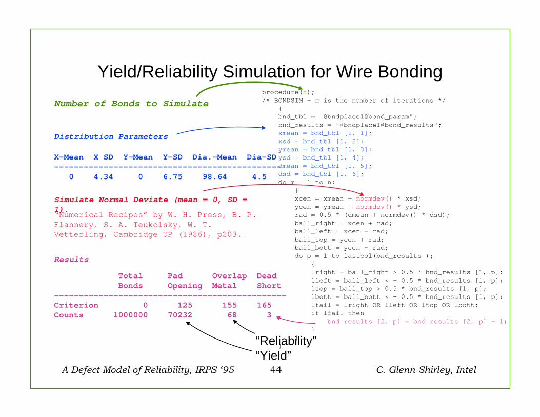
Yield/Reliability Simulation for Wire Bonding
Total Pad Overlap DeadBonds Opening Metal Short
-----------------------------------------------Criterion 0 125 155 165Counts 1000000 70232 68 3
X-Mean X SD Y-Mean Y-SD Dia.-Mean Dia-SD----------------------------------------------
0 4.34 0 6.75 98.64 4.5
procedure(n);/* BONDSIM - n is the number of iterations */
{bnd_tbl = "@bndplace1@bond_param";bnd_results = "@bndplace1@bond_results";xmean = bnd_tbl [1, 1];xsd = bnd_tbl [1, 2];ymean = bnd_tbl [1, 3];ysd = bnd_tbl [1, 4];dmean = bnd_tbl [1, 5];dsd = bnd_tbl [1, 6];do m = 1 to n;
{xcen = xmean + normdev() * xsd;ycen = ymean + normdev() * ysd;rad = 0.5 * (dmean + normdev() * dsd);ball_right = xcen + rad;ball_left = xcen - rad;ball_top = ycen + rad;ball_bott = ycen - rad;do p = 1 to lastcol(bnd_results );
{lright = ball_right > 0.5 * bnd_results [1, p];lleft = ball_left < - 0.5 * bnd_results [1, p];ltop = ball_top > 0.5 * bnd_results [1, p];lbott = ball_bott < - 0.5 * bnd_results [1, p];lfail = lright OR lleft OR ltop OR lbott;if lfail then
bnd_results [2, p] = bnd_results [2, p] + 1;}
}}
Number of Bonds to Simulate
Distribution Parameters
“Numerical Recipes” by W. H. Press, B. P. Flannery, S. A. Teukolsky, W. T. Vetterling, Cambridge UP (1986), p203.
Simulate Normal Deviate (mean = 0, SD = 1).
Results
“Reliability”“Yield”
A Defect Model of Reliability, IRPS ‘95 45 C. Glenn Shirley, Intel
Scaling of Defect Reliability: Summary• Yield and reliability defect densities may be calculated,
simulated, or measured, but...• The model requires an assumption (or null hypothesis) of
– Random, non interacting defects.– An invariant ratio of Yield to Reliability defect densities.
• The defect-related part of the survival function scales with the density of latent reliability defects and die (or affected subdie) area.
• By hypothesis, yield and reliability defect densities are proportional, so the defect part of the survival function ALSO scales with yield defect density.
• The “practical” form of the model involves sort yield and sort Pareto data. Simplification obtains if yield defect Paretos are invariant.
A Defect Model of Reliability, IRPS ‘95 46 C. Glenn Shirley, Intel
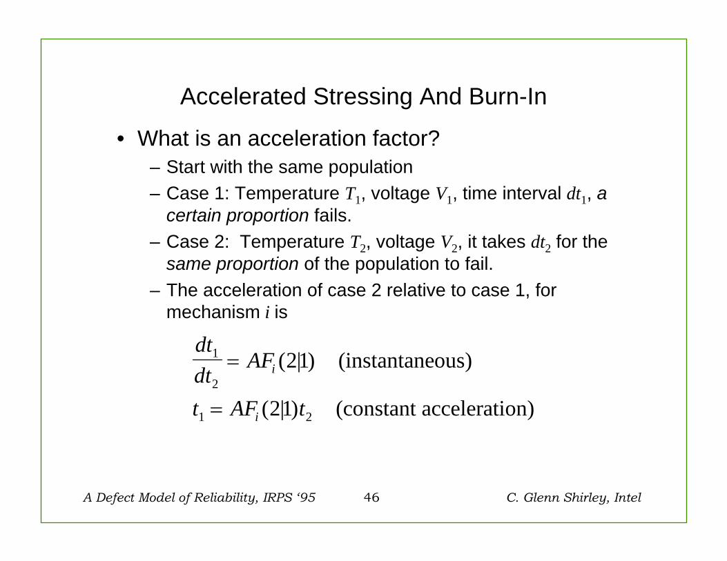
Accelerated Stressing And Burn-In
• What is an acceleration factor?– Start with the same population– Case 1: Temperature T1, voltage V1, time interval dt1, a
certain proportion fails.– Case 2: Temperature T2, voltage V2, it takes dt2 for the
same proportion of the population to fail.– The acceleration of case 2 relative to case 1, for
mechanism i is
dtdt
AF
t AF t
i
i
1
2
1 2
21
21
=
=
( | )
( | )
(instantaneous)
(constant acceleration)
A Defect Model of Reliability, IRPS ‘95 47 C. Glenn Shirley, Intel
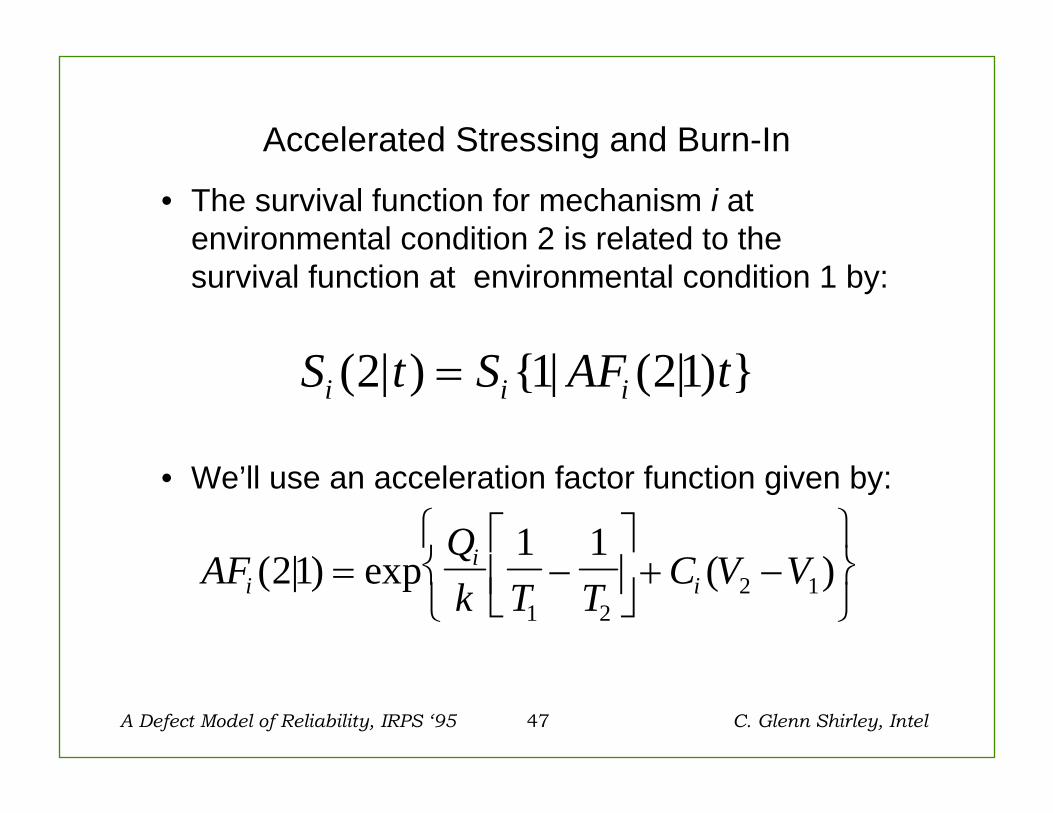
Accelerated Stressing and Burn-In
• The survival function for mechanism i at environmental condition 2 is related to the survival function at environmental condition 1 by:
• We’ll use an acceleration factor function given by:
S t S AF ti i i( | ) { | ( | ) }2 1 21=
AFQk T T
C V Vii
i( | ) exp ( )211 1
1 22 1= −
⎡
⎣⎢⎤
⎦⎥+ −
⎧⎨⎩
⎫⎬⎭
A Defect Model of Reliability, IRPS ‘95 48 C. Glenn Shirley, Intel
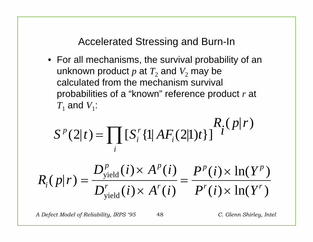
Accelerated Stressing and Burn-In
• For all mechanisms, the survival probability of an unknown product p at T2 and V2 may be calculated from the mechanism survival probabilities of a “known” reference product r at T1 and V1:
S t S AF tRi p r
pir
ii
( | ) [ { | ( | ) }]( | )
2 1 21= ∏
R p rD i A iD i A i
P i YP i Yi
p p
r r
p p
r r( | )( ) ( )( ) ( )
( ) ln( )( ) ln( )
=×
×=
××
yield
yield
A Defect Model of Reliability, IRPS ‘95 49 C. Glenn Shirley, Intel
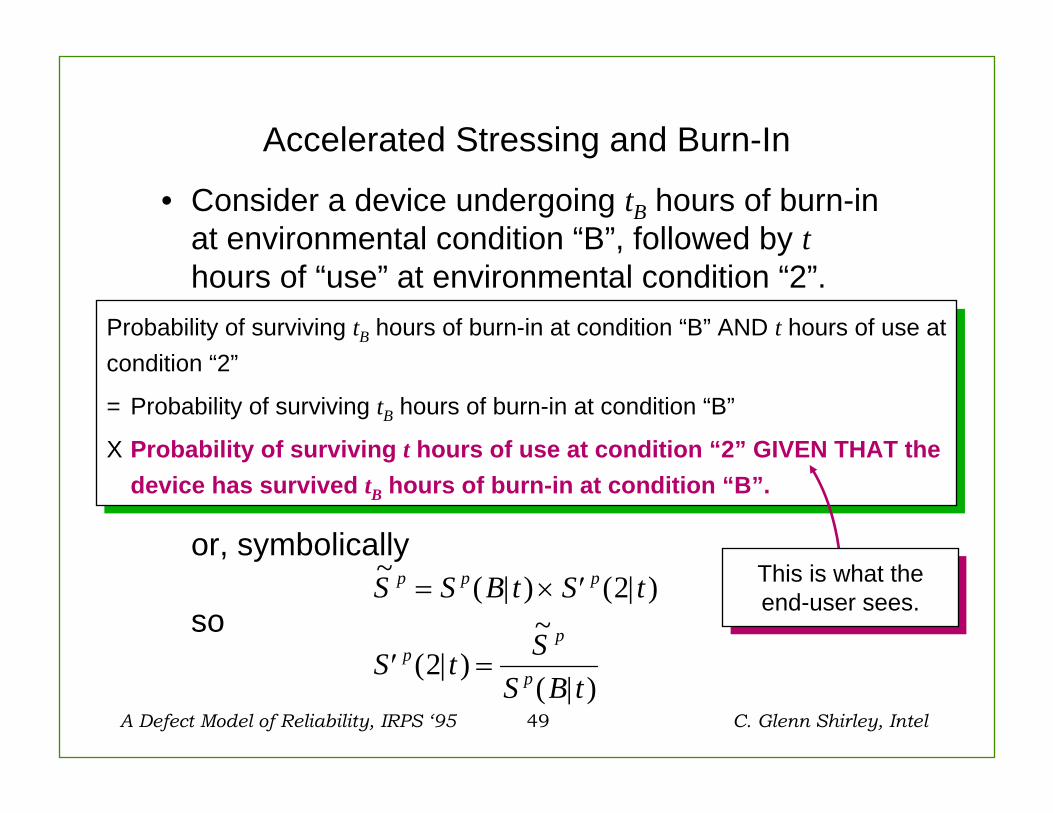
Accelerated Stressing and Burn-In
• Consider a device undergoing tB hours of burn-in at environmental condition “B”, followed by thours of “use” at environmental condition “2”.
or, symbolically
so
Probability of surviving tB hours of burn-in at condition “B” AND t hours of use at condition “2”
= Probability of surviving tB hours of burn-in at condition “B”
X Probability of surviving t hours of use at condition “2” GIVEN THAT the device has survived tB hours of burn-in at condition “B”.
Probability of surviving tB hours of burn-in at condition “B” AND t hours of use at condition “2”
= Probability of surviving tB hours of burn-in at condition “B”
X Probability of surviving t hours of use at condition “2” GIVEN THAT the device has survived tB hours of burn-in at condition “B”.
~ ( | ) ( | )
( | )~
( | )
S S B t S t
S t SS B t
p p p
pp
p
= × ′
′ =
2
2
This is what the end-user sees.
This is what the end-user sees.
A Defect Model of Reliability, IRPS ‘95 50 C. Glenn Shirley, Intel
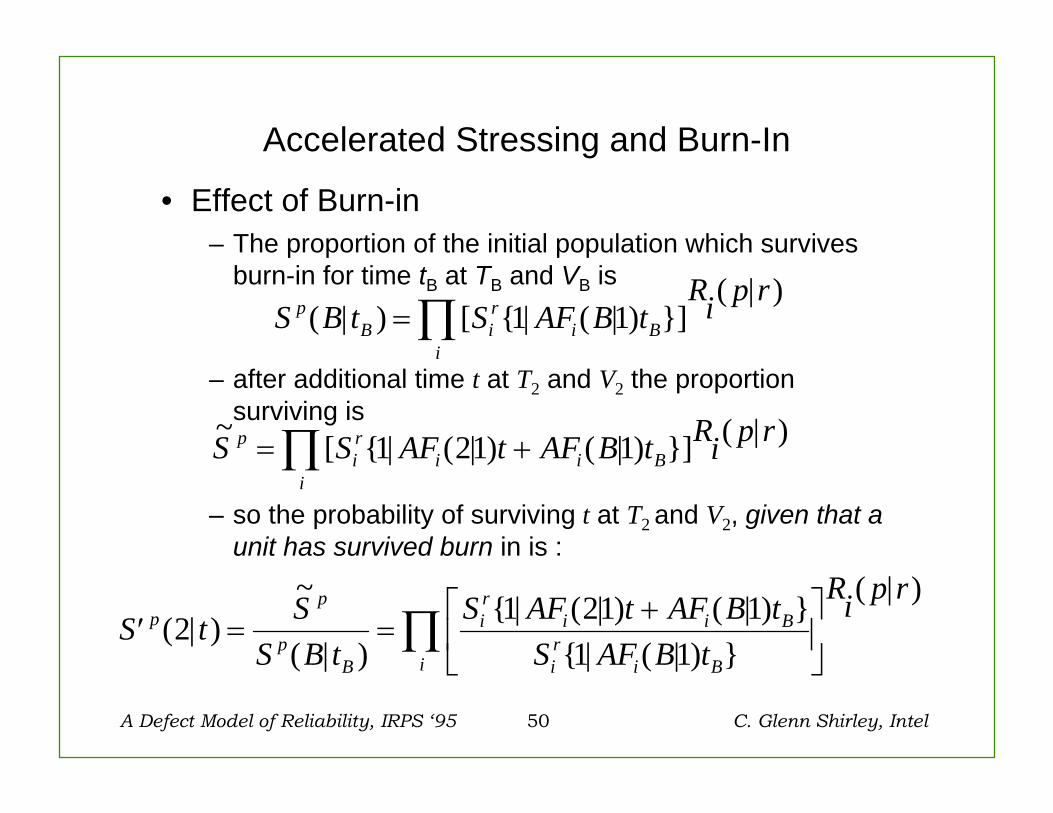
Accelerated Stressing and Burn-In
• Effect of Burn-in– The proportion of the initial population which survives
burn-in for time tB at TB and VB is
– after additional time t at T2 and V2 the proportion surviving is
– so the probability of surviving t at T2 and V2, given that a unit has survived burn in is :
S B t S AF B tRi p r
pB i
ri
iB( | ) [ { | ( | ) }]
( | )= ∏ 1 1
~ [ { | ( | ) ( | ) }] ( | )S S AF t AF B t Ri p rpir
i i Bi
= +∏ 1 21 1
′ = =+⎡
⎣⎢
⎤
⎦⎥∏S t S
S B tS AF t AF B t
S AF B t
Ri p rp
p
pB
ir
i i B
ir
i Bi
( | )~
( | ){ | ( | ) ( | ) }
{ | ( | ) }
( | )2 1 21 1
1 1
A Defect Model of Reliability, IRPS ‘95 51 C. Glenn Shirley, Intel
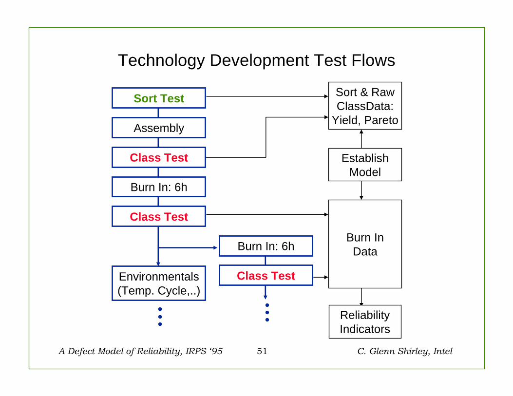
Technology Development Test Flows
Class Test
Assembly
Sort Test
Class Test
Burn In: 6h
Environmentals(Temp. Cycle,..)
Class Test
Burn In: 6hBurn In
Data
Sort & RawClassData:
Yield, Pareto
EstablishModel
ReliabilityIndicators
A Defect Model of Reliability, IRPS ‘95 52 C. Glenn Shirley, Intel
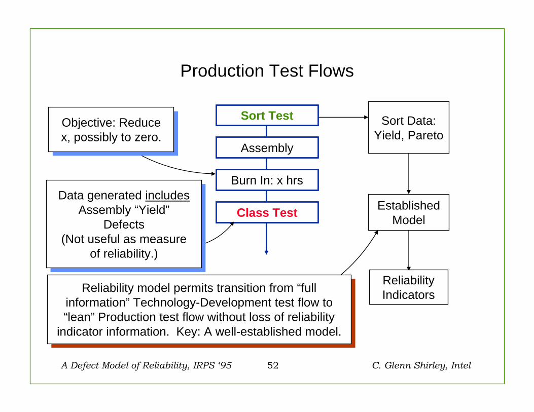
Production Test Flows
Assembly
Sort Test
Class Test
Burn In: x hrs
Sort Data:Yield, Pareto
ReliabilityIndicators
EstablishedModel
Objective: Reduce x, possibly to zero.
Objective: Reduce x, possibly to zero.
Data generated includesAssembly “Yield”
Defects(Not useful as measure
of reliability.)
Data generated includesAssembly “Yield”
Defects(Not useful as measure
of reliability.)
Reliability model permits transition from “full information” Technology-Development test flow to “lean” Production test flow without loss of reliability
indicator information. Key: A well-established model.
Reliability model permits transition from “full information” Technology-Development test flow to “lean” Production test flow without loss of reliability
indicator information. Key: A well-established model.

A Defect Model of Reliability, IRPS ‘95 53 C. Glenn Shirley, Intel
Test Programs
• Sort test is a wafer-level room temperature test.
• Class test is a unit level test using temperature-controlled hander.
• Sort and Class tests can stressunits, particularly the high-voltage test.
– Nominal temperature/volts is done last.
– The stress in the test must be taken account of in low voltage burn-in (for acceleration studies).
Typical Class TestTemperatures:
Hot: 90 CCold: -10 C
RoomVoltages:
LowHigh
Nominal
Typical Sort TestTemperatures:
RoomVoltages:
LowHigh
A Defect Model of Reliability, IRPS ‘95 54 C. Glenn Shirley, Intel
Analysis of Reliability Data• How do we get the “reference” survival function?• Production burn-in data and extended life test data
from a variety of products fabricated using a specific process are accumulated. This body of data is the “baseline lot” reliability data.
• Baseline data is consolidated using “known”acceleration models and defect scaling to produce a “reference lot” reliability data.
• Reference lot data is calculated at single reference values of defect density, die area, temperature and bias.
• Parametric fits to reference lot data gives “reference model distributions”.

A Defect Model of Reliability, IRPS ‘95 55 C. Glenn Shirley, Intel
Analysis of Reliability Data
Lot 1Area1, DD1, Tj1, V1
Lot 2
Area2, DD2, Tj2, V2
Lot N
AreaN, DDN, TjN, VN. . . . . . . .
SCALE TO ONE REFERENCE AREA, DD, Tj, and V
BASELINE LOT DATA
REFERENCE LOT DATAat reference values of
Area, DD, Tj, V
(DD = Yield Defect Density)

A Defect Model of Reliability, IRPS ‘95 56 C. Glenn Shirley, Intel
Typical Minimum Data Requirements for Determination of Process Reference Models
• 4 lots of SRAM, 4000 units at V = 140% of nominal, and 125C.
• Several lots at other bias/voltage conditions to determine acceleration parameters.
– nominal bias, room temperature– sometimes assign Q, C based on “known” mechanism.
• All lots Class tested before burn-in (“clean burn-in”)• Readouts at 6, 48, 168, 500, 1000, 2000 hours.• Known Yield and Defect Pareto for each lot.• All failures validated, all failure signatures traceable to
a physically analyzed failure.– “A Q and a C for every failure”.
A Defect Model of Reliability, IRPS ‘95 57 C. Glenn Shirley, Intel
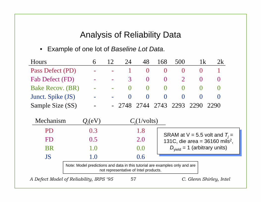
Analysis of Reliability Data• Example of one lot of Baseline Lot Data.
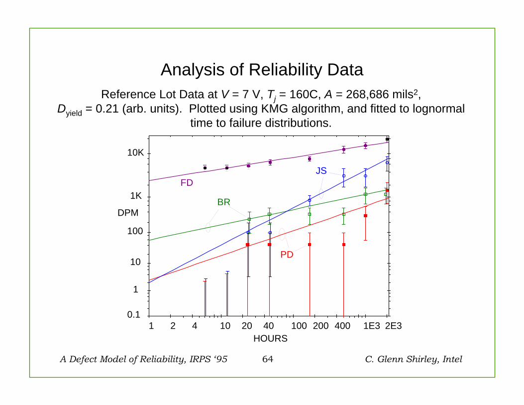
Hours 6 12 24 48 168 500 1k 2kPass Defect (PD) - - 1 0 0 0 0 1Fab Defect (FD) - - 3 0 0 2 0 0Bake Recov. (BR) - - 0 0 0 0 0 0Junct. Spike (JS) - - 0 0 0 0 0 0Sample Size (SS) - - 2748 2744 2743 2293 2290 2290
PD 0.3 1.8FD 0.5 2.0BR 1.0 0.0JS 1.0 0.6
Mechanism Qi(eV) Ci(1/volts)
SRAM at V = 5.5 volt and Tj = 131C, die area = 36160 mils2,
Dyield = 1 (arbitrary units)
SRAM at V = 5.5 volt and Tj = 131C, die area = 36160 mils2,
Dyield = 1 (arbitrary units)
Note: Model predictions and data in this tutorial are examples only and arenot representative of Intel products.
A Defect Model of Reliability, IRPS ‘95 58 C. Glenn Shirley, Intel
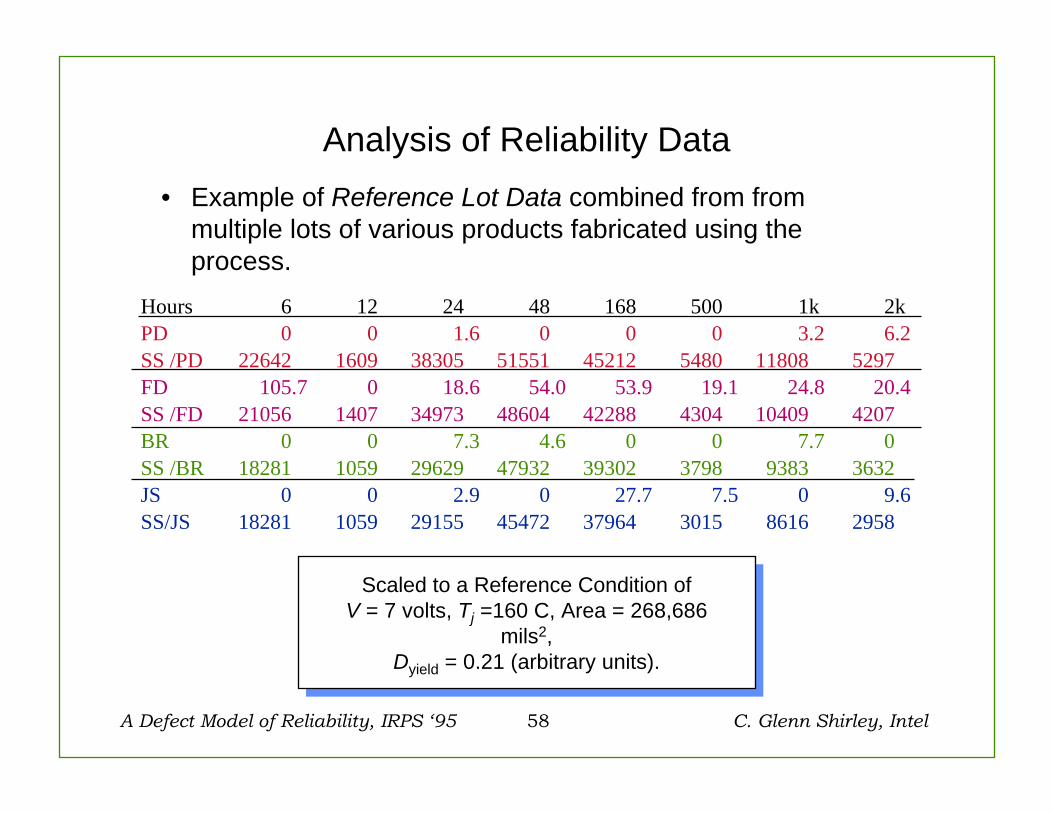
Analysis of Reliability Data• Example of Reference Lot Data combined from from
multiple lots of various products fabricated using the process.
Hours 6 12 24 48 168 500 1k 2kPD 0 0 1.6 0 0 0 3.2 6.2SS /PD 22642 1609 38305 51551 45212 5480 11808 5297FD 105.7 0 18.6 54.0 53.9 19.1 24.8 20.4SS /FD 21056 1407 34973 48604 42288 4304 10409 4207BR 0 0 7.3 4.6 0 0 7.7 0SS /BR 18281 1059 29629 47932 39302 3798 9383 3632JS 0 0 2.9 0 27.7 7.5 0 9.6SS/JS 18281 1059 29155 45472 37964 3015 8616 2958
Scaled to a Reference Condition ofV = 7 volts, Tj =160 C, Area = 268,686
mils2,Dyield = 0.21 (arbitrary units).
Scaled to a Reference Condition ofV = 7 volts, Tj =160 C, Area = 268,686
mils2,Dyield = 0.21 (arbitrary units).
A Defect Model of Reliability, IRPS ‘95 59 C. Glenn Shirley, Intel
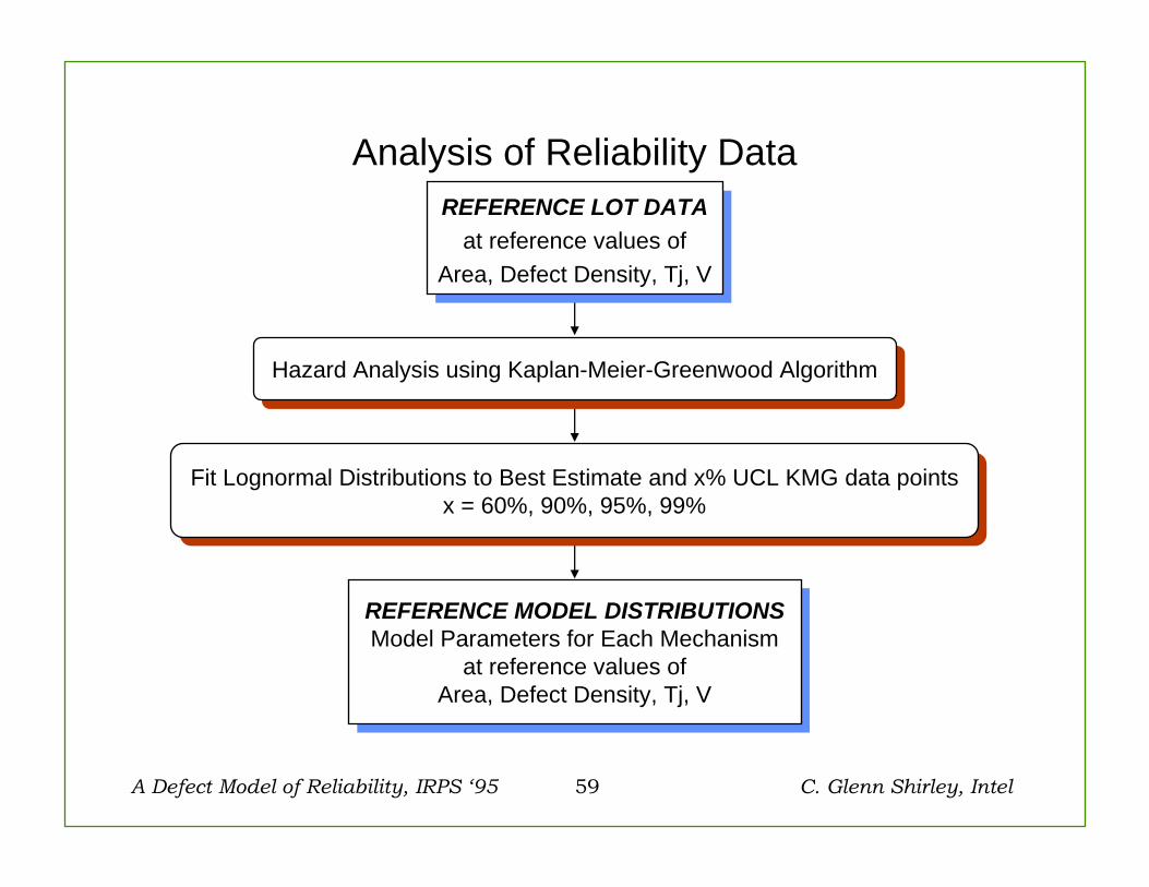
Analysis of Reliability DataREFERENCE LOT DATA
at reference values ofArea, Defect Density, Tj, V
REFERENCE LOT DATAat reference values of
Area, Defect Density, Tj, V
Hazard Analysis using Kaplan-Meier-Greenwood AlgorithmHazard Analysis using Kaplan-Meier-Greenwood Algorithm
Fit Lognormal Distributions to Best Estimate and x% UCL KMG data pointsx = 60%, 90%, 95%, 99%
Fit Lognormal Distributions to Best Estimate and x% UCL KMG data pointsx = 60%, 90%, 95%, 99%
REFERENCE MODEL DISTRIBUTIONSModel Parameters for Each Mechanism
at reference values ofArea, Defect Density, Tj, V
REFERENCE MODEL DISTRIBUTIONSModel Parameters for Each Mechanism
at reference values ofArea, Defect Density, Tj, V

A Defect Model of Reliability, IRPS ‘95 60 C. Glenn Shirley, Intel
Statistical Interlude: Hazard Analysis
• Data produced by burn-in and life-test flows is nearly always censored (has removals).
– Because material is diverted into other stresses in TD.– Because failures are often invalidated.– Because of multiple failure mechanisms.
• A simple method of analysis. For each mechanism:
– Calculate instantaneous hazard.– Find cumulative hazard.– Use F = 1-exp(-H) to find cumulative failures.– Plot F vs time on log probability plot.
A Defect Model of Reliability, IRPS ‘95 61 C. Glenn Shirley, Intel
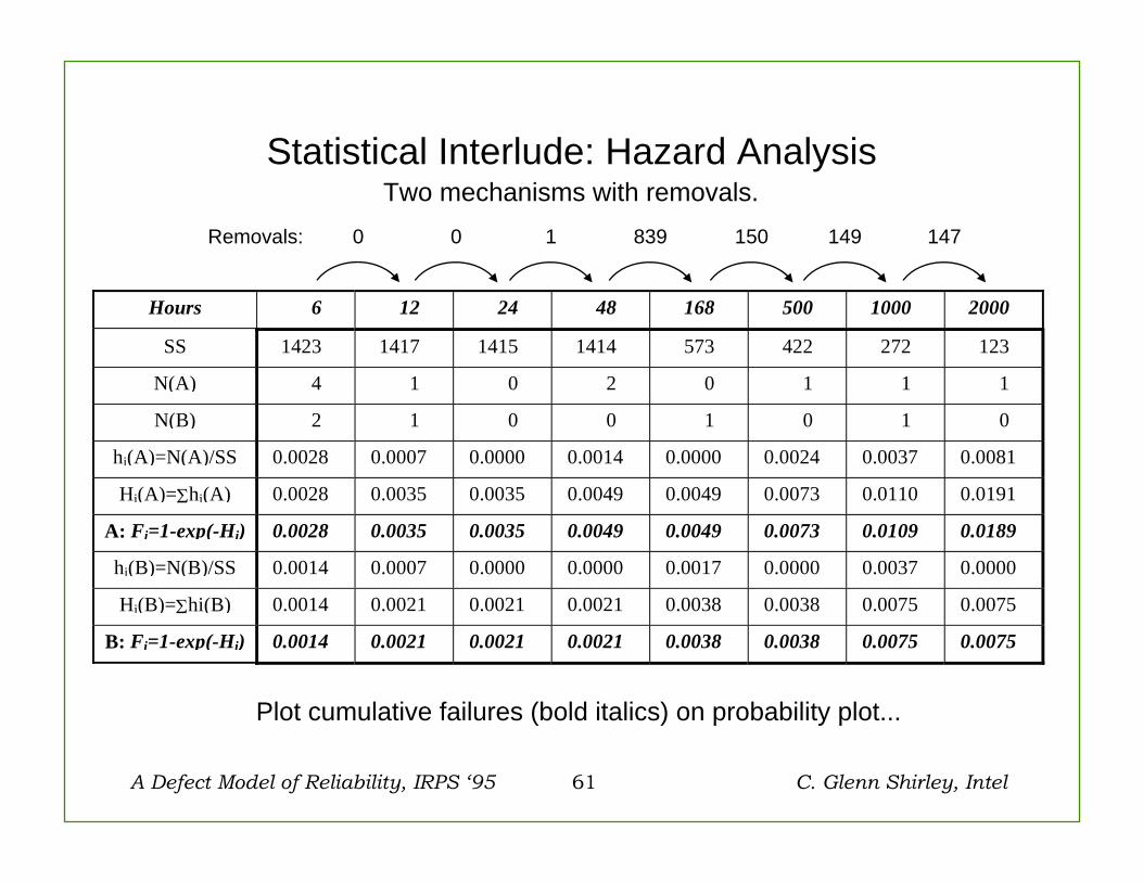
Hours 6 12 24 48 168 500 1000 2000
SS 1423 1417 1415 1414 573 422 272 123
N(A) 4 1 0 2 0 1 1 1
N(B) 2 1 0 0 1 0 1 0
hi(A)=N(A)/SS 0.0028 0.0007 0.0000 0.0014 0.0000 0.0024 0.0037 0.0081
Hi(A)=Σhi(A) 0.0028 0.0035 0.0035 0.0049 0.0049 0.0073 0.0110 0.0191
A: Fi=1-exp(-Hi) 0.0028 0.0035 0.0035 0.0049 0.0049 0.0073 0.0109 0.0189
hi(B)=N(B)/SS 0.0014 0.0007 0.0000 0.0000 0.0017 0.0000 0.0037 0.0000
Hi(B)=Σhi(B) 0.0014 0.0021 0.0021 0.0021 0.0038 0.0038 0.0075 0.0075
B: Fi=1-exp(-Hi) 0.0014 0.0021 0.0021 0.0021 0.0038 0.0038 0.0075 0.0075
1 839 150 149 1470 0Removals:
Two mechanisms with removals.
Plot cumulative failures (bold italics) on probability plot...
Statistical Interlude: Hazard Analysis
A Defect Model of Reliability, IRPS ‘95 62 C. Glenn Shirley, Intel
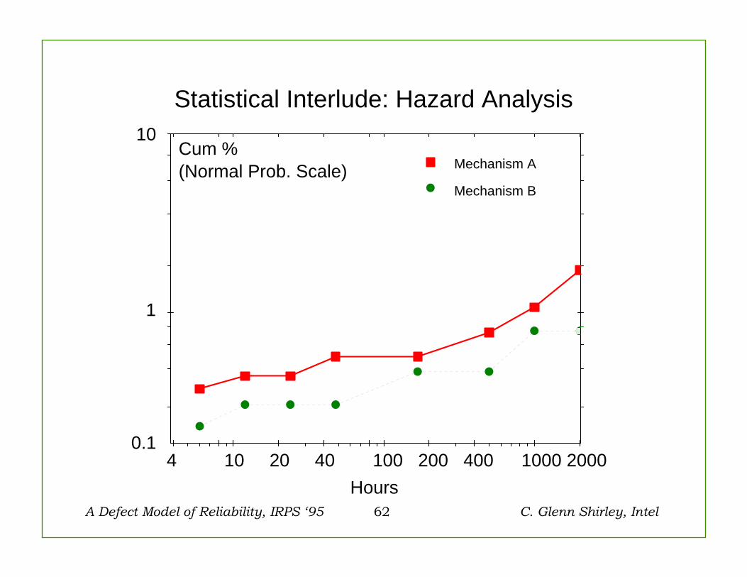
4 10 20 40 100 200 400 1000 2000
1
10
0.1
Hours
Cum %(Normal Prob. Scale) Mechanism A
Mechanism B
Statistical Interlude: Hazard Analysis

A Defect Model of Reliability, IRPS ‘95 63 C. Glenn Shirley, Intel
Analysis of Reliability Data
• The Kaplan-Meier-Greenwood (KMG) method handles censored readout data and provides confidence intervals. See Nelson*.
• Plot, lognormally, KMG estimates of cum fails. • Least-squares fit of straight line through KMG
plot points provides statistical model parameters.
y F x t
t
i i i i= =
= = − ×
=
−Φ 1
50
1
( ); ln( )
/
exp( )
slope; intercept σ μ σ
μ* W. Nelson, “Accelerated Testing,” John Wiley & Sons (1989), pp 145-151.
Inverse Normal Probability Function
Inverse Normal Probability Function
A Defect Model of Reliability, IRPS ‘95 64 C. Glenn Shirley, Intel
Analysis of Reliability Data
1 2 4 10 20 40 100 200 400 1E3 2E30.1
1
10
100
1K
10K
DPM
HOURS
PD
JSFD
BR
Reference Lot Data at V = 7 V, Tj = 160C, A = 268,686 mils2, Dyield = 0.21 (arb. units). Plotted using KMG algorithm, and fitted to lognormal
time to failure distributions.
A Defect Model of Reliability, IRPS ‘95 65 C. Glenn Shirley, Intel
Analysis of Reliability Data
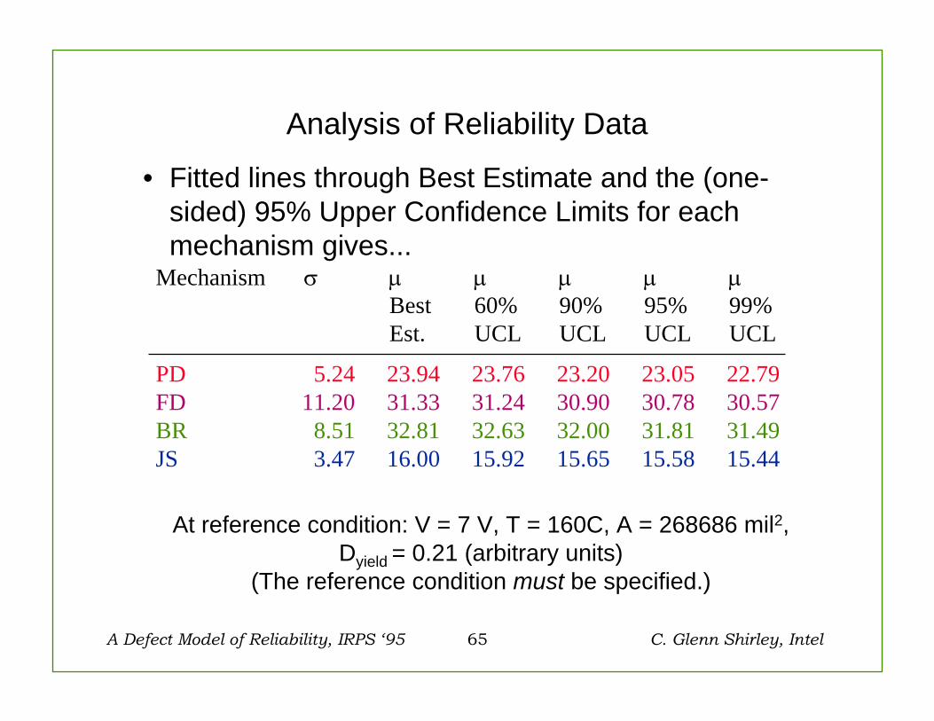
• Fitted lines through Best Estimate and the (one-sided) 95% Upper Confidence Limits for each mechanism gives...
PD 5.24 23.94 23.76 23.20 23.05 22.79FD 11.20 31.33 31.24 30.90 30.78 30.57BR 8.51 32.81 32.63 32.00 31.81 31.49JS 3.47 16.00 15.92 15.65 15.58 15.44
Mechanism σ μ μ μ μ μBest 60% 90% 95% 99%Est. UCL UCL UCL UCL
At reference condition: V = 7 V, T = 160C, A = 268686 mil2,Dyield = 0.21 (arbitrary units)
(The reference condition must be specified.)

A Defect Model of Reliability, IRPS ‘95 66 C. Glenn Shirley, Intel
Analysis of Reliability Data
• Substitution of parameters into the lognormal distribution gives the “reference” survival function at time t in environmental condition “2” for the process:
where μ and σ for the mechanism are known at the reference condition “1”.
• This would be substituted, for example, into
S t AF tir i i
i
( | ) ln[ ( | ) ]2 1 21= −
−⎛⎝⎜
⎞⎠⎟Φ
μσ
S t S AF tRi p r
pir
ii
( | ) [ { | ( | ) }]( | )
2 1 21= ∏ R p r P i YP i Yi
p p
r r( | ) ( ) ln( )( ) ln( )
=××
A Defect Model of Reliability, IRPS ‘95 67 C. Glenn Shirley, Intel
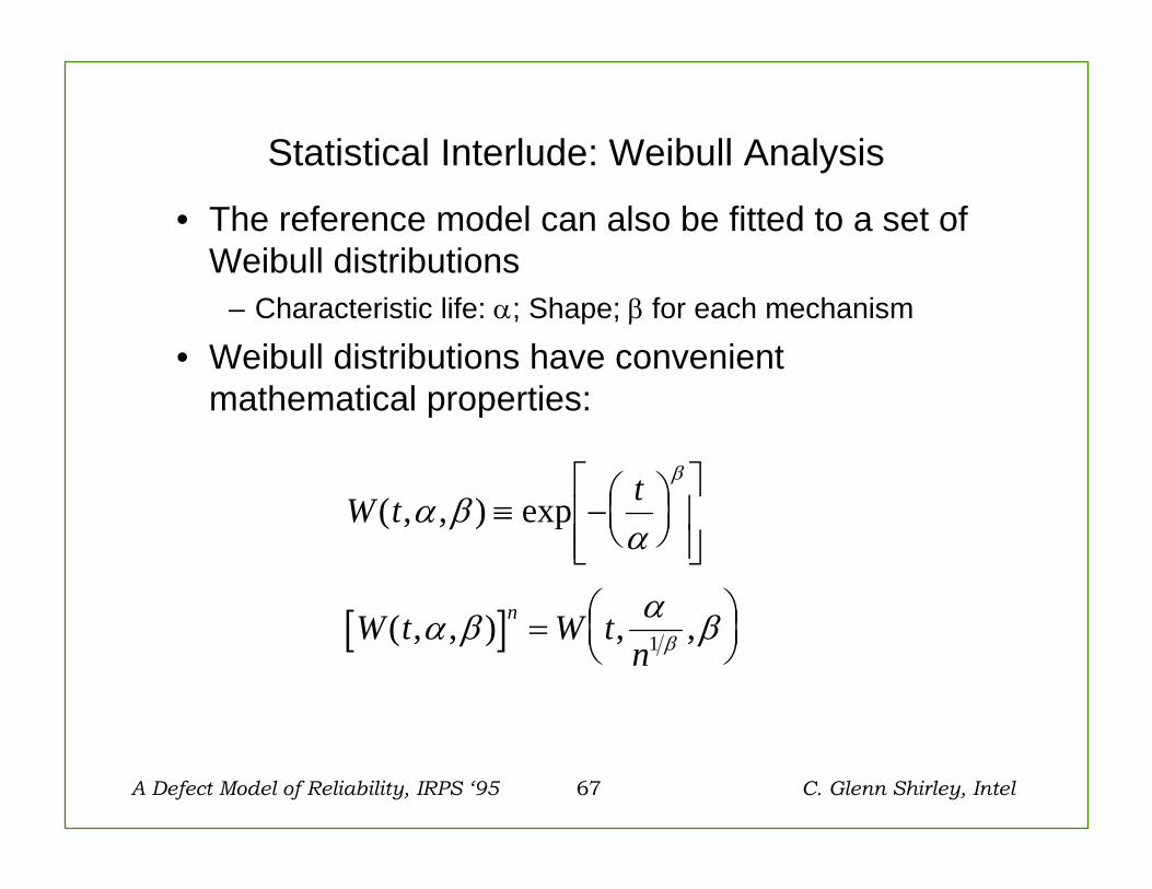
Statistical Interlude: Weibull Analysis
• The reference model can also be fitted to a set of Weibull distributions
– Characteristic life: α; Shape; β for each mechanism
• Weibull distributions have convenient mathematical properties:
[ ]
W t t
W t W tn
n
( , , ) exp
( , , ) , ,
α βα
α β α β
β
β
≡ −⎛⎝⎜
⎞⎠⎟
⎡
⎣⎢⎢
⎤
⎦⎥⎥
= ⎛⎝⎜
⎞⎠⎟1
A Defect Model of Reliability, IRPS ‘95 68 C. Glenn Shirley, Intel
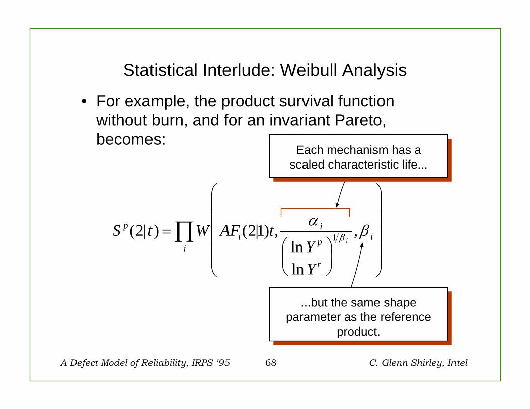
Statistical Interlude: Weibull Analysis
• For example, the product survival function without burn, and for an invariant Pareto, becomes:
S t W AF tYY
pi
i
p
r
ii
i( | ) ( | ) ,
lnln
,2 21 1=⎛⎝⎜
⎞⎠⎟
⎛
⎝
⎜⎜⎜⎜⎜
⎞
⎠
⎟⎟⎟⎟⎟
∏ α ββ
...but the same shape parameter as the reference
product.
...but the same shape parameter as the reference
product.
Each mechanism has a scaled characteristic life...Each mechanism has a
scaled characteristic life...
A Defect Model of Reliability, IRPS ‘95 69 C. Glenn Shirley, Intel
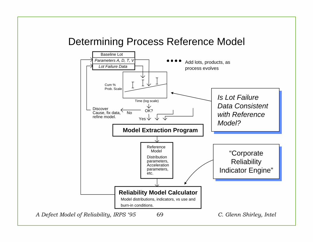
Determining Process Reference ModelBaseline Lot
Lot Failure DataParameters A, D, T, V
Time (log scale)
Cum %Prob. Scale
Model Extraction Program
OK?NoDiscoverCause, fix data,
Yes
Add lots, products, asprocess evolves
refine model.
Reliability Model CalculatorModel distributions, indicators, vs use andburn-in conditions.
ReferenceModel
Distributionparameters,Accelerationparameters,etc.
Is Lot Failure Data Consistent with Reference Model?
Is Lot Failure Data Consistent with Reference Model?
“Corporate Reliability
Indicator Engine”
“Corporate Reliability
Indicator Engine”
A Defect Model of Reliability, IRPS ‘95 70 C. Glenn Shirley, Intel
Refinement of Process Reference Models
• Add product lots to baseline lot set.– Reveal mechanisms missed by SRAM model.
• Check for consistency with reference model.– Some lots class tested at a single-point (6 hr, 125C,
140%V), full F/A, known lot iso, at a minimum.– If failure rates are higher than predicted by model, a
“red flag” is indicated.
• Refine the reference model– Re-extract using Model Extraction Software.– Re-extract and install model
» Immediately if change is significant.» On annual cycle if product is consistent with model.
A Defect Model of Reliability, IRPS ‘95 71 C. Glenn Shirley, Intel
Reliability Prediction
• Effect of burn in on SRAM reliability.
• Model predictions vs individual lot data from baseline data set.
• Calculation of standard reliability indicators.
A Defect Model of Reliability, IRPS ‘95 72 C. Glenn Shirley, Intel
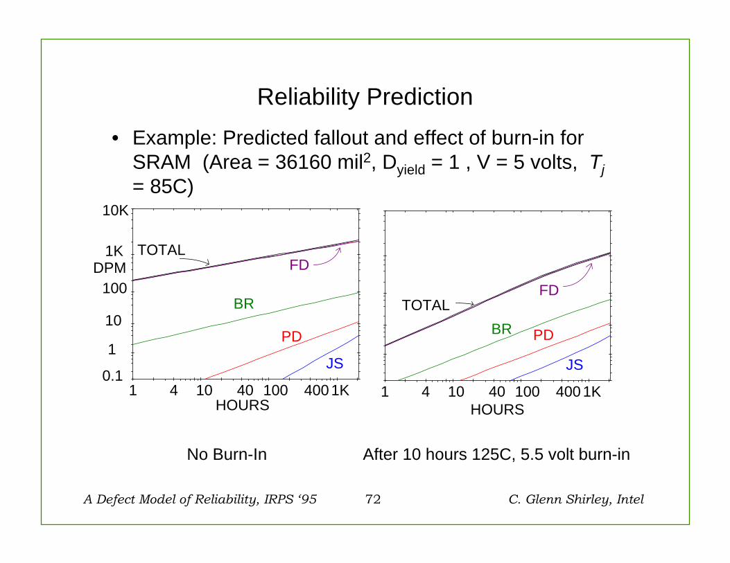
Reliability Prediction• Example: Predicted fallout and effect of burn-in for
SRAM (Area = 36160 mil2, Dyield = 1 , V = 5 volts, Tj= 85C)
1 4 10 40 100 400 1K0.1
1
10
100
1K
10K
DPM
HOURS
TOTALFD
BR
PD
JS
1 4 10 40 100 400 1KHOURS
TOTALFD
BR PD
JS
No Burn-In After 10 hours 125C, 5.5 volt burn-in

A Defect Model of Reliability, IRPS ‘95 73 C. Glenn Shirley, Intel
Reliability Prediction
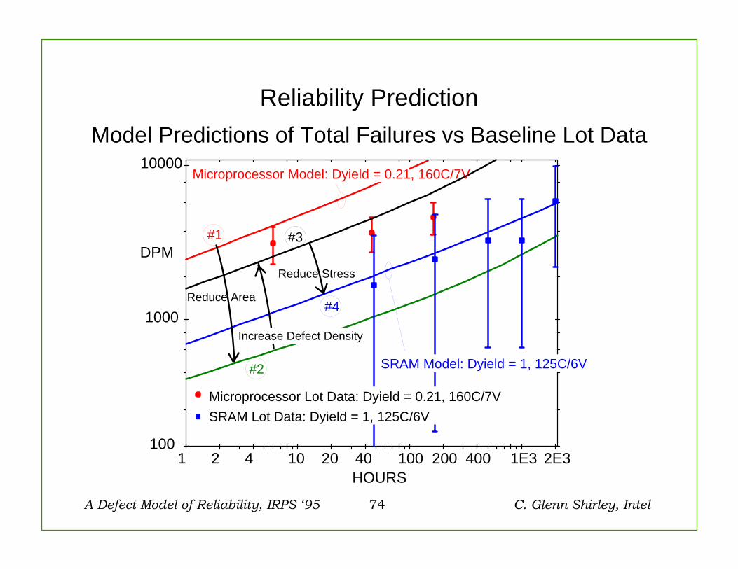
• Model predictions of the reference model based on the entire baseline lot data set versusindividual data sets selected from the baseline data set.
• A sequence of conditions ranging from conditions of microprocessor data for a particular lot to conditions of SRAM data for a particular lot...
Note: Model predictions and data are examples only and arenot representative of Intel products.
1 268,686 0.21 160 7 Microprocessor lot data2 36,160 0.21 160 73 36,160 1.00 160 74 36,160 1.00 125 6 SRAM lot data
No. A(mil2) Dyld T(C) V(volts)
A Defect Model of Reliability, IRPS ‘95 74 C. Glenn Shirley, Intel
Reliability Prediction
1 2 4 10 20 40 100 200 400 1E3 2E3100
1000
10000
DPM
HOURS
Reduce Area
Reduce Stress
#1
#2
#3
#4
SRAM Model: Dyield = 1, 125C/6V
Microprocessor Lot Data: Dyield = 0.21, 160C/7VSRAM Lot Data: Dyield = 1, 125C/6V
Microprocessor Model: Dyield = 0.21, 160C/7V
Increase Defect Density
Model Predictions of Total Failures vs Baseline Lot Data
A Defect Model of Reliability, IRPS ‘95 75 C. Glenn Shirley, Intel
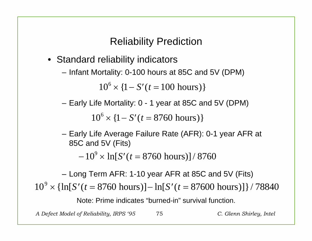
Reliability Prediction
• Standard reliability indicators– Infant Mortality: 0-100 hours at 85C and 5V (DPM)
– Early Life Mortality: 0 - 1 year at 85C and 5V (DPM)
– Early Life Average Failure Rate (AFR): 0-1 year AFR at 85C and 5V (Fits)
– Long Term AFR: 1-10 year AFR at 85C and 5V (Fits)
10 1 1006 × − ′ ={ ( )}S t hours
10 1 87606 × − ′ ={ ( )}S t hours
− × ′ =10 8760 87609 ln[ ( ] /S t hours)
10 8760 87600 788409 × ′ = − ′ ={ln[ ( )] ln[ ( )]} /S t S t hours hoursNote: Prime indicates “burned-in” survival function.
A Defect Model of Reliability, IRPS ‘95 76 C. Glenn Shirley, Intel
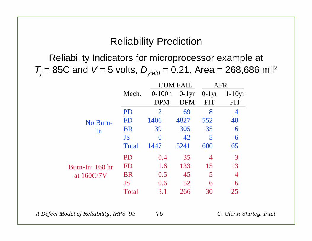
Reliability PredictionReliability Indicators for microprocessor example at
Tj = 85C and V = 5 volts, Dyield = 0.21, Area = 268,686 mil2
No Burn-In
Burn-In: 168 hrat 160C/7V
PD 2 69 8 4FD 1406 4827 552 48BR 39 305 35 6JS 0 42 5 6Total 1447 5241 600 65PD 0.4 35 4 3FD 1.6 133 15 13BR 0.5 45 5 4JS 0.6 52 6 6Total 3.1 266 30 25
CUM FAIL AFRMech. 0-100h 0-1yr 0-1yr 1-10yr
DPM DPM FIT FIT

A Defect Model of Reliability, IRPS ‘95 77 C. Glenn Shirley, Intel
Benefits• Estimation of the reliability characteristics of any
product, including the contributions of various mechanisms.
• Estimation of failure rates of complex products without full reliance on failure analysis, or complete data.
• Estimation of the effect of die area, array area, etc. on the reliability characteristics of any proposed or new product using no, or minimal, data.
• Quantify the reliability benefits of process continuous improvement through defect density reduction.
• Calculate the effect of burn-in.• Calculate reliability indicators useful to customers, at
any desired level of confidence.
A Defect Model of Reliability,: Clustering Effects, IRPS ‘95 C. Glenn Shirley, Intel 1
Supplementary Slides on Clustering Effects

A Defect Model of Reliability,: Clustering Effects, IRPS ‘95 C. Glenn Shirley, Intel 2
Effects of Defect Clustering
• Random defects:
• Clustered defects:
= +
Total DefectDensity
Yield DefectDensity
ReliabilityDefect Density
= +
Total DefectDensity
Yield DefectDensity
ReliabilityDefect Density
A Defect Model of Reliability,: Clustering Effects, IRPS ‘95 C. Glenn Shirley, Intel 3
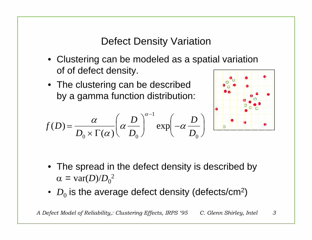
Defect Density Variation
• Clustering can be modeled as a spatial variation of of defect density.
• The clustering can be describedby a gamma function distribution:
• The spread in the defect density is described by α = var(D)/D0
2
• D0 is the average defect density (defects/cm2)
f DD
DD
DD
( )( )
exp=×
⎛⎝⎜
⎞⎠⎟ −
⎛⎝⎜
⎞⎠⎟
−α
αα α
α
0 0
1
0Γ
A Defect Model of Reliability,: Clustering Effects, IRPS ‘95 C. Glenn Shirley, Intel 4
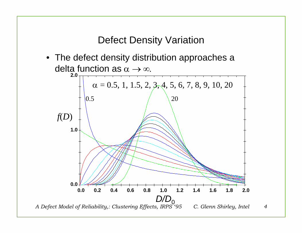
Defect Density Variation
• The defect density distribution approaches a delta function as α → ∞.
0.0 0.2 0.4 0.6 0.8 1.0 1.2 1.4 1.6 1.8 2.0 0.0
1.0
2.0
200.5
D/D0
f(D)
α = 0.5, 1, 1.5, 2, 3, 4, 5, 6, 7, 8, 9, 10, 20

A Defect Model of Reliability,: Clustering Effects, IRPS ‘95 C. Glenn Shirley, Intel 5
Yield Function with Clustering
• The yield function is the probability of occurrence of one defect on a die of area A:
• In the limit of no clustering (uniform D), this becomes
Y DA f D dDD A
= − =+⎛
⎝⎜⎞⎠⎟
∞
∫ exp( ) ( ) 1
1 00
α
α
1
1 00
+⎛⎝⎜
⎞⎠⎟
⎯ →⎯⎯ −→∞D AD A
α
α α exp( )

A Defect Model of Reliability,: Clustering Effects, IRPS ‘95 C. Glenn Shirley, Intel 6
Yield Function with Clustering
• Clustering of defects gives higher yields than predicted by random defect model...
0.0 1.0 2.0 3.0
.4
.8
1
20
0.5
α = 0.5, 1, 1.5, 2, 3, 4, 5, 6, 7, 8, 9, 10, 20
Yield
D0A
A Defect Model of Reliability,: Clustering Effects, IRPS ‘95 C. Glenn Shirley, Intel 7
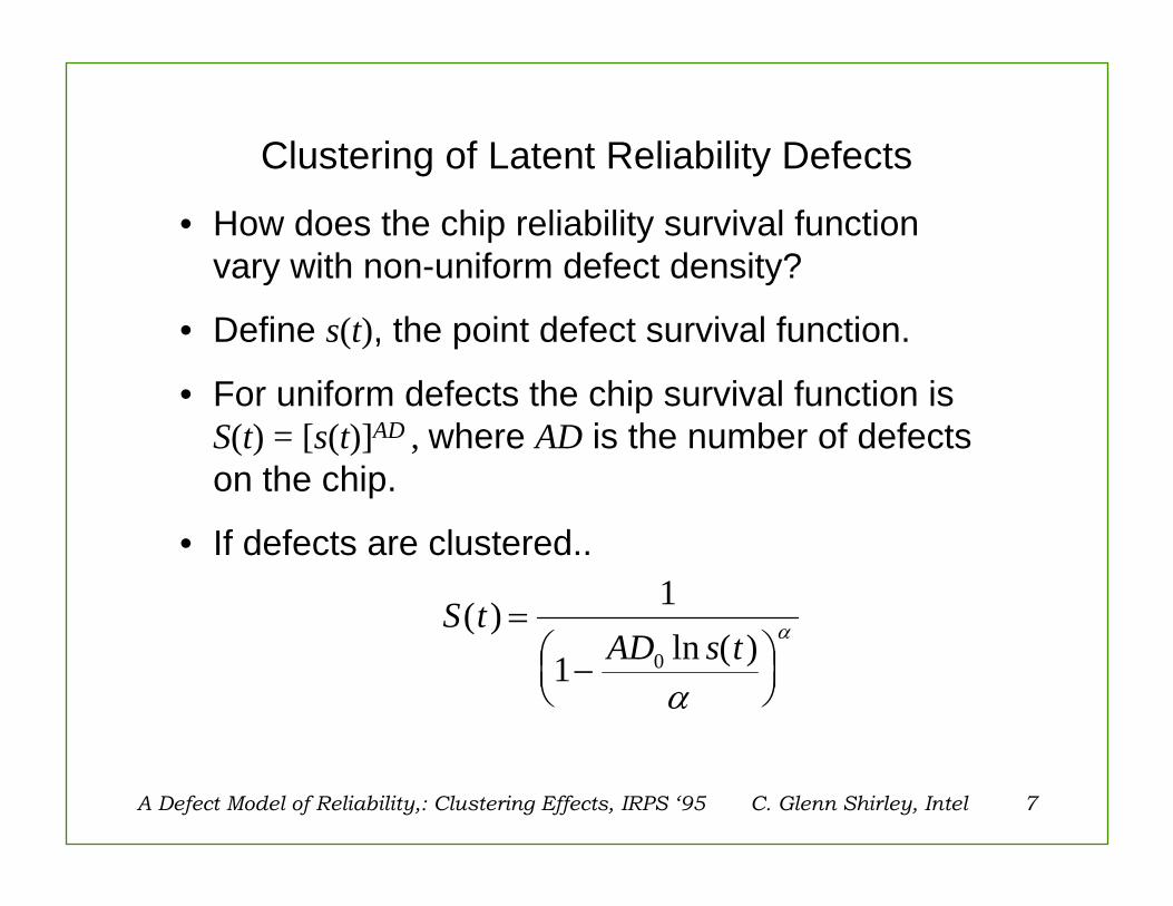
Clustering of Latent Reliability Defects
• How does the chip reliability survival function vary with non-uniform defect density?
• Define s(t), the point defect survival function.
• For uniform defects the chip survival function isS(t) = [s(t)]AD , where AD is the number of defects on the chip.
• If defects are clustered..
S tAD s t
( )ln ( )
=−⎛
⎝⎜⎞⎠⎟
1
1 0
α
α
A Defect Model of Reliability,: Clustering Effects, IRPS ‘95 C. Glenn Shirley, Intel 8
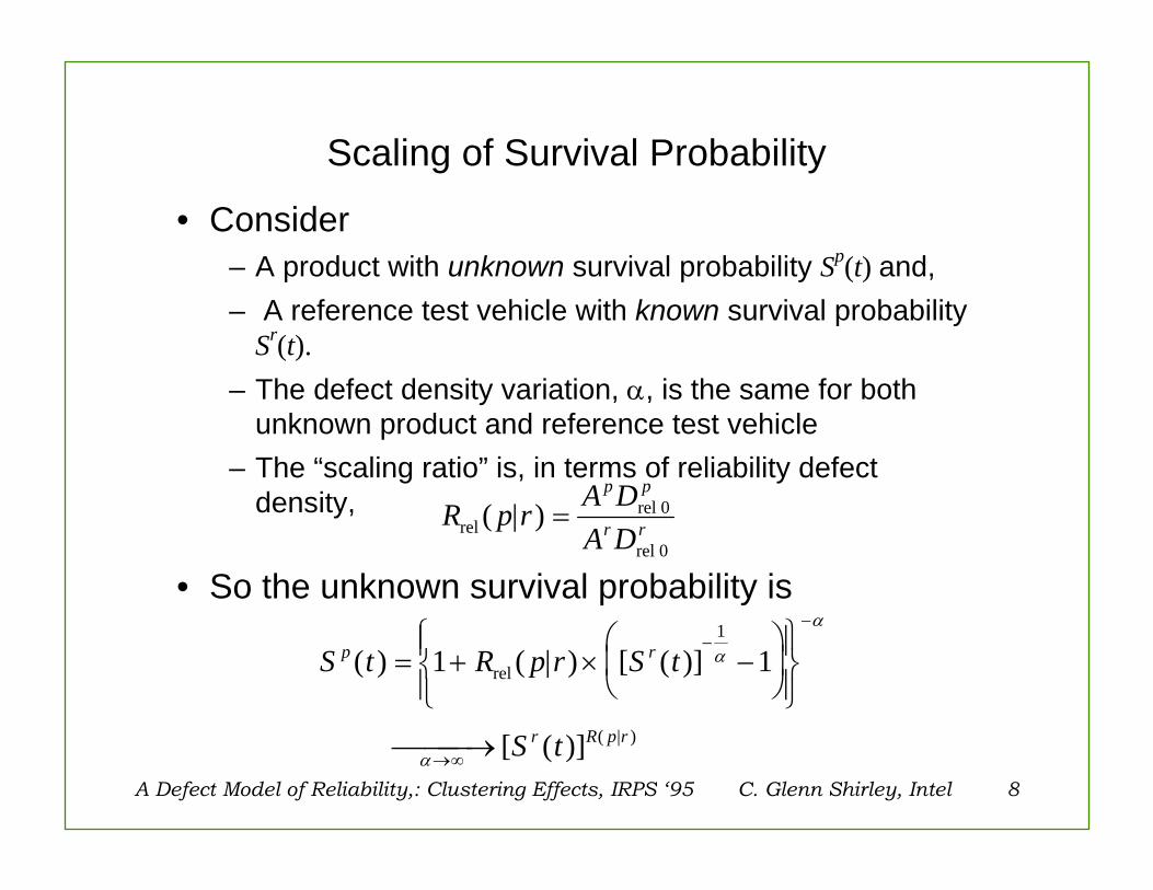
Scaling of Survival Probability
• Consider– A product with unknown survival probability Sp(t) and,– A reference test vehicle with known survival probability
Sr(t).– The defect density variation, α, is the same for both
unknown product and reference test vehicle– The “scaling ratio” is, in terms of reliability defect
density,
• So the unknown survival probability is
S t R p r S t
S t
p r
r R p r
( ) ( | ) [ ( )]
[ ( )] ( | )
= + × −⎛
⎝⎜
⎞
⎠⎟
⎧⎨⎪
⎩⎪
⎫⎬⎪
⎭⎪
⎯ →⎯⎯
−−
→∞
1 11
relα
α
α
R p r A DA D
p p
r rrelrel 0
rel 0
( | ) =
A Defect Model of Reliability,: Clustering Effects, IRPS ‘95 C. Glenn Shirley, Intel 9
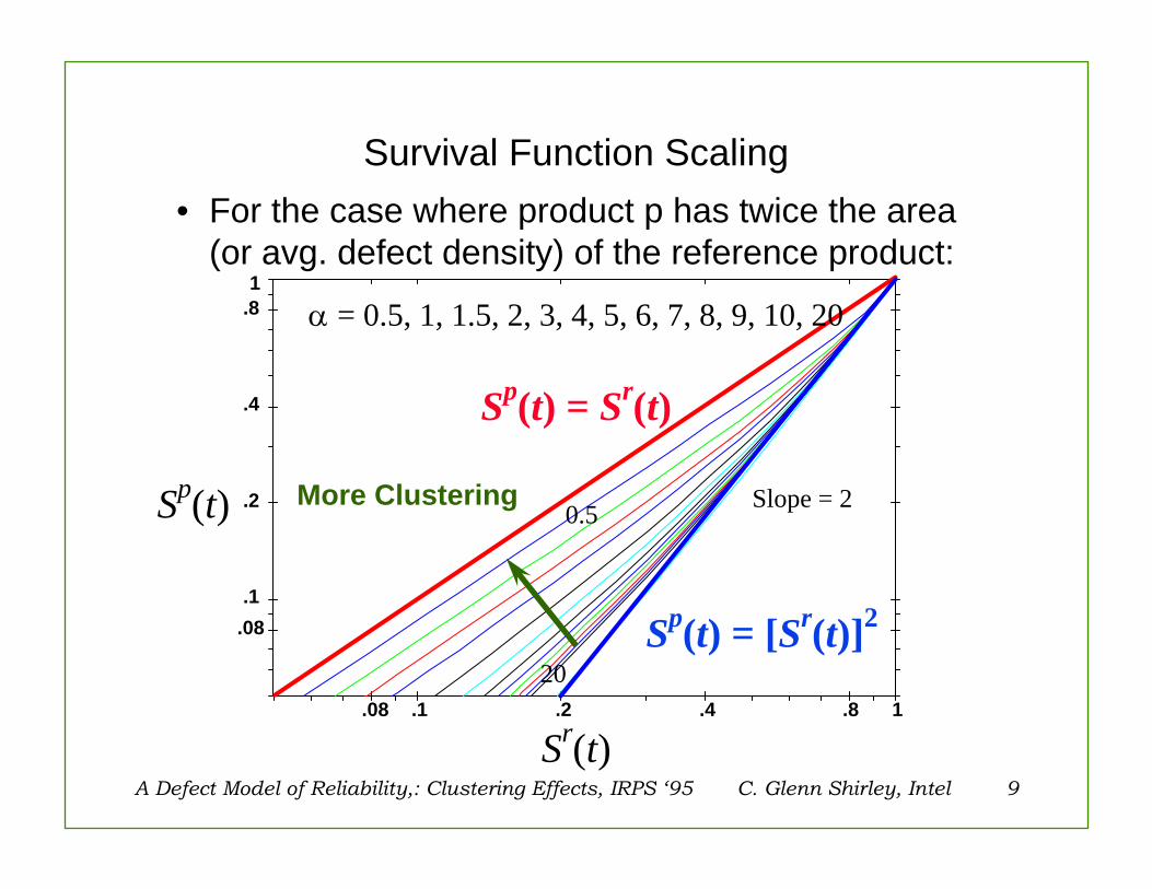
Survival Function Scaling
.08 .1 .2 .4 .8 1
.08 .1
.2
.4
.8 1
20
0.5 Slope = 2
α = 0.5, 1, 1.5, 2, 3, 4, 5, 6, 7, 8, 9, 10, 20
• For the case where product p has twice the area (or avg. defect density) of the reference product:
Sp(t)
Sr(t)
Sp(t) = Sr(t)
Sp(t) = [Sr(t)]2
More Clustering

A Defect Model of Reliability,: Clustering Effects, IRPS ‘95 C. Glenn Shirley, Intel 10
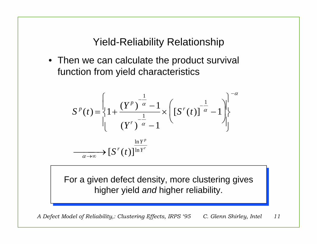
Yield-Reliability Relationship
• From the yield formulae
• I f we make the fundamental assumption
• And assume the dispersion in reliability and yield defect densities are the same
R p rA DA D
Y
Y
YY
p p
r r
p
r
p
ryieldyield 0
yield 0
( | ) ( )
( )
lnln
= =−
−⎯ →⎯⎯
−
− →∞
1
11
1
α
αα
R p rA DA D
A DA D
R p rp p
r r
p p
r rreliabilityreliability 0
reliability 0
yield 0
yield 0yield( | ) ( | )= ≅ =
α α α= ≅reliability yield
A Defect Model of Reliability,: Clustering Effects, IRPS ‘95 C. Glenn Shirley, Intel 11
Yield-Reliability Relationship
• Then we can calculate the product survival function from yield characteristics
S t Y
YS t
S t
pp
r
r
rYY
p
r
( ) ( )
( )[ ( )]
[ ( )]lnln
= +−
−× −
⎛
⎝⎜
⎞
⎠⎟
⎧
⎨⎪
⎩⎪
⎫
⎬⎪
⎭⎪
⎯ →⎯⎯
−
−
−
−
→∞
1 1
11
1
1
1α
α
α
α
α
For a given defect density, more clustering gives higher yield and higher reliability.
For a given defect density, more clustering gives higher yield and higher reliability.

A Defect Model of Reliability,: Clustering Effects, IRPS ‘95 C. Glenn Shirley, Intel 12
Extension to Multiple Mechanisms
S t Y
YS t
P Y
P YS t
S t
p ip
ir
ir
i
ip p
ir r
ir
i
ir
PP
i
YY
i
i
i
i
ip
ir
p
r
( ) ( )
( )[ ( )]
[( ) ]
[( ) ][ ( )]
( )
lnln
= +−
−
× −⎛
⎝⎜⎜
⎞
⎠⎟⎟
⎧
⎨⎪
⎩⎪
⎫
⎬⎪
⎭⎪
= +−
−× −
⎛
⎝⎜
⎞
⎠⎟
⎧⎨⎪
⎩⎪
⎫⎬⎪
⎭⎪
⎯ →⎯⎯⎛
⎝⎜⎜
⎞
⎠⎟⎟
−
−
−
−
−
−
−
−
→∞
∏
∏
∏
1 1
11
1 1
11
1
1
1
1
1
1
α
α
α
α
α
α
α
α
α
Y p and Y r are the total yields (all mechanisms).
P pi and P ri are yield Paretos.
α is the defect density dispersion parameter (all mechanisms)
Y p and Y r are the total yields (all mechanisms).
P pi and P ri are yield Paretos.
α is the defect density dispersion parameter (all mechanisms)