A Demometric Analysis of Ulpian´s Table

A Demometric Analysis of Ulpian’s Table

Peter Pflaumer1 1Department of Statistics, Technical University of Dortmund

Abstract Ulpian’s table is a famous ancient text that is preserved in edited form in Justinian’s Digest, a compendium of Roman law compiled by order of the emperor Justinian I in the sixth century AD. This passage probably provides a rough estimation of Roman life expectancy in the early third century AD. The paper begins with a discussion of the demographic properties and peculiarities of Ulpian´s table. Then the Gompertz distri-bution and some of its extensions are used to fit life expectation functions to Ulpian´s data. The model can be used to estimate important demographic functions and parameters of the Roman life table. Inter alia, the average and median remaining life expectancies are calculated, and compared with the results of other investigations, e.g., Frier’s life table for the Roman Empire. It turns out that Ulpian´s life table is characterized by a steep decline of the life expectancy function in the advanced age classes, which is much steeper than in life expectancy functions of other life tables based on data. The modal or normal age at death, which is between 55 and 60 years, is comparatively high. Key Words: Life Table, Mortality Law, Gompertz-Makeham, Roman Demography

1. Introduction

Almost all historians now assume that Roman life expectancy at birth was approximately 25 years (see, e.g., Frier 2000, p. 788). One source for Roman mortality figures is Ulpian’s table. This table was a tool to compute the capital value of a legacy of alimenta, taking into account the age of the legatee (see, e.g., Sanchez-Moreno Ellart, 2013). It is the first methodological mortality table known to man, and was not only written but also used in legal practice, although life expectancy certainly fluctuated from period to period, region to region, and class to class. Ulpian’s table is the first piece of evidence for calculating the value of life annuities on a rational basis. In medieval Europe, the prices of life annuities were typically quoted without reference to age. It still took a long time until the bases for the calculations for life annuities were known. In the seventeenth century, the Dutch prime minister Jan de Witt (1625-1672) and the famous astronomer Edmond Halley (1656-1742) calculated the correct premiums for life annuities for the first time.

2. Ulpian’s table and its analysis

Domitius Ulpianus was a famous Roman jurist who lived in the second century AD. He was also a Prefect of the Praetorian Guard. Ulpian was killed by his enemies in the Praetorian Guard in 228. Under Justinian I, Roman emperor from 527 to 565, the existing Roman law was compiled. The Digest (Digesta) was one part of the “Corpus Juris Civilis”, the body of the civil law. The Digest, published in 533, consists of extracts from leading jurists organized by subject. In about one third of the texts Ulpian is quoted. His

JSM 2014 - Social Statistics Section

405

brought to you by COREView metadata, citation and similar papers at core.ac.uk

provided by Eldorado - Ressourcen aus und für Lehre, Studium und Forschung

https://core.ac.uk/display/46916048?utm_source=pdf&utm_medium=banner&utm_campaign=pdf-decoration-v1

writings survive only in these extracts within the Digest. The particular extract of interest by Ulpian is that quoted by Aemilius Macer, a Roman jurist, who wrote after the time of Ulpian. One of his works is “Ad Legem de Vicesima Hereditatum” (On the Law of the Twentieth Portion of an Inheritance). This mainly deals with a commentary on the “Lex Julia de Vicesima Hereditatum”, an Augustan law of 6 AD that put a 5% tax on inheritances. Macer’s text provides a scheme presented by Ulpian to compute tax for life-time annuities and usufructs (Frier 1982). Ulpian’s scheme can be summarized as a table which illustrates the relation between age and the present value of a life-time annuity of one. If the interest rate is zero, which is in general assumed, the present value corresponds to the life expectancy at age x. Ulpian’s table is often associated with the Falcidian Law of 40 BC (cf., e.g., Müller 1906, De Vries & Zwalve 2004, Mays 1971a), which is named after the Roman Tribune Falcidius. This law prevented testators giving more than 75% of their wealth as life annuities to third parties; a testator was obliged to leave at least one fourth of his estate to his heirs. In this use, the table should estimate the so-called “quarta Falcidia” (but see Parkin 1992 pp. 29ff. or Frier 1982 for a complete interpretation of that passage in Macer’s writing). Roman lawyers could obtain the value of a life-time annuity or a usufruct by multiplying its annual value by the appropriate factor at age x ( see Table 1). Table 1: Ulpian’s table Age x [0,20) [20,25) [25,30) [30,35) [35,40) [40,50) [50,55) [55,60) 60+ Life expectancy at age x

30 28 25 22 20 59 - x 9 7 5

In most cases, the life expectancy at age x in Ulpian’s table is regarded as the average number of years lived after age x, which in continuous form is given by: 0 1

( ) ( )( )

= ∫e x l z dzl x x

ω,

where l(x) is the ratio of people who survive to age x, with l(0)=1 and ω the maximum age. Some researchers (e.g., De Vries & Zwalve 2004, Dupaquier 1973, Frier 1982) consider the life expectancy to be the median life expectancy1 (median or probable length of life) at age x. This is the number of years elapsed before half of the population of age x has died. Formally, the median life expectancy e(x) can be computed by: l(x e(x))

0.5l(x)+

= .

Figure 1 shows a graphical representation of Ulpian’s table. Ulpian’s table is a step function. The jump discontinuities are -2 at ages 20, 35, 55, and 60. They are -3 at ages 25 and 30, and between the ages of 40 and 50 they are -1. These jump discontinuities are not realistic, since the decrease in life expectancy at an age x cannot exceed 1.

1 Strictly speaking, the expression mean or average life expectancy is a pleonasm (because mean is the same as expectation), whereas the expression median life expectancy is an inconsistency (median is not mean). However, I often use these two expressions in order to distinguish clearly between the two interpretations of the figures in Ulpian’s table.


406

20 30 40 50 60 70

05

1015

2025

30

Age x

Life

exp

ecta

ncy

at a

ge x

Figure 1: Ulpian’s table as a step function

A well-known relationship exists between the mean life expectancy 0e(x) and the force of

mortality (x)μ :

0ed (x)1dx(x) 0

0e(x)

+μ = ≥ ,

which implies that 0ed (x)

1dx

= − if (x) 0μ = .

Assuming a Gompertz distribution with k>0 (see section 4), it is possible to show a similar result for the median life expectancy at age x: de(x) 1

(x)dx 1k ln 2

= − μ+

⋅

.

If (x) 0μ = then de(x)1

dx= − ; for the modal age x=m the derivative is:

de(x) 1(x)dx 1

k ln2

= − μ+

⋅

= 1k 1

k ln 2

−+

⋅

= 10.4091 1

ln 2

− ≈ −+

.

If we approximate Ulpian’s table by a continuous linear function between the ages of 40

and 50, then an unrealistic result of a zero mortality rate appears, since 0ed (x)

1dx

= − (see

Figure 2, lower part). Ciecka (2012) shows this fact for a discrete life table in which the life expectancy at age x decreases by one year. Zero mortality rates at these ages were probably not intended by the originators of Ulpian’s table. Why should they assume this in the light of their daily evidence about deaths in this age class? Therefore, we suppose a


407

step function in this age class (with a one-year length), too. In this case, the force of

mortality is a step function with 1(x)

0e(x)μ = , since

0ed (x)0

dx= (see Figure 2, upper part).

Figure 3 compares the force of mortality function of Ulpian’s table with the functions of Süssmilch’s life table and a life table produced from Roman epitaph information. Johann Peter Süssmilch (1707-1767), one of the founding fathers of demography in Germany, published a life table with a life expectancy at birth of about 29 years2. His life table represents the typical European mortality situation in the eighteenth century. The force of mortality function has been calculated with the age-specific death probabilities qx, using

( )(x) ln 1 qxμ = − − . The Roman mortality pattern has been obtained from the data of 9,980 epitaphs, which were collected by Szilágyi (1963). The force of mortality was estimated from age-specific death rates and was then smoothed by the hazard rate function of the Gompertz distribution (x) A exp(k x)μ = ⋅ ⋅ with A=0.0312 and k=0.0165.

Figure 2: Force of mortality functions of Ulpian’s table

2 Süssmilch, J P (1775): Die göttliche Ordnung in den Veränderungen des menschlichen Geschlechts, aus der

Geburt, dem Tode, und der Fortpflanzung erwiesen, 4. Ausgabe, Berlin.


408

0 10 20 30 40 50 60 70

0.00

0.05

0.10

0.15

0.20

Age x

Forc

e of

mor

talit

y

UlpianSüßmilchRome

Figure 3: Comparison of different force of mortality functions (Ulpian’s table, Süssmilch’s life table, Roman epitaph population life table)

We will begin our comparison with Frier’s (1982) answer to Hopkins’ (1966) criticism that the table is not demographically possible. “In one sense it is undeniable that Ulpian’s table is not demographically possible, at least if we apply to it modern standard. Life expectancy obviously does not drop in rigid quinquennial leaps, nor does it keep to integers of years. But these are relatively trivial matters, more style than substance” (Frier 1982, p. 229). Frier sees it as a problem that the table does not realistically reflect life expectancy for infant and child mortality, for mortality between 40 and 60 years of age or for mortality after the age of 60. The reasons for these demographic inconsistencies, according to Frier, could be the difficulties with data collection in the classes of the very young and the very old, or the fact that the young age classes may easily have been ignored, because children do not usually receive annuities. Langner (1998, p. 308) mentions that the decision on the survival of a newborn child in Rome lay within the family and was not subject to public law. Thus infant mortality cannot be compared with today’s definition. Therefore it is not appropriate to begin the table with the age of zero. The table is valid at the earliest from the age of one. The zero mortality rates between 40 and 50 are an unintentional result, and only arise if one takes a continuous linear function. The results disappear if one assumes a step function. The problem would not have arisen if the creators of the table had proposed a step function with only one constant value between the ages of 40 and 50. If we ignore infant mortality, the main difference between Ulpian’s table and an eighteenth century life table is the higher mortality from the age of 5 and the steep mortality increase from the age of 45 (see Figure 3). Up to the age of 40 the force of mortality functions from Ulpian’s table and from a Roman epitaph population are very


409

similar. Is this an indication that the compilers of Ulpian’s table partly used genuine data from tombstones in Roman cemeteries, as De Vries and Zwalve (2004) assume? How can the unusually steep increase be explained? Is the mortality increase beyond the age of 45 based on empirical data or on the ancient idea that life ends at the age of 70 or 80? Solon’s verses on the ten ages of man end with … “But if he completes ten ages of seven years each, full measure, death, when it comes, can no longer be said to come too soon”. Solon, Athens’ first great statesman, composed these verses about 600 BC. He fixed the life span with ten seven-year periods, and in his view old age begins in the ninth seven-year period, that is after the age of 56 years (see “The Works of Philo”). In the Bible the psalmist put it as follows (Ps. 90:10): “The days of our lives are seventy years; And if by reason of strength they are eighty years, Yet their boast is only labor and sorrow; For it is soon cut off, and we fly away”. These views about life span were widely held in Antiquity3 . In summary, Ulpian’s table is, in a strict sense, not a demographically correct mortality table. But it was not designed for demographic purposes. It aimed to estimate the value of annuities and usufructs; and it had to be accurate only within the legal limits of its use (Frier 1982, p. 230). The most striking fact is the steep increase of the force of mortality, or the probability of death, in the advanced age classes. This steep increase causes a steep decline in the life expectancy function. This decline is much steeper than in life expectancy functions of other life tables based on data. Nothing is written about the origin of Ulpian’s table. It is not known whether Ulpian himself was the originator of the table. Hildebrand (1866) believes that Ulpian’s table is based on statistical bases because of the legal background to its use. De Vries and Zwalve (2004, p. 297) are convinced that Ulpian’s table was a deliberate attempt to construct a fairly accurate life expectancy table using simple mathematical methods, and that the compilers of the table must have used genuine demographic data. However, Hopkins (1966) writes that Ulpian’s table is neither empirically based nor demographically possible. Parkin (1992, pp. 38-39) states that there is no evidence for, and no need to see, an empirical basis for the figures that are given; they are based on good guesswork. Ulpian’s table was the topic of many investigations over the years. Niklaus Bernoulli discusses Ulpian’s table at length in Chapter V of his doctoral dissertation “De Usu Artis Conjectandi in Jure” as early as 1709 (Kohli 1975). Ulpian’s table was the official annuity table of the Tuscan Government in Northern Italy until early in the nineteenth century (Kopf 1926).

3. Frier’s life table

Frier describes his life table construction in detail (see Frier 1982 pp. 238ff.). He uses a two-stage estimation procedure. In the first stage, he fits two exponential curves to Ulpian’s data. The first curve is a regression for ages 15 to 50, and the second is a regression for ages 40 to 70. He determines specific survivorship rates l(x) from these curves, assuming that Ulpian’s values are median life expectancies. In the second stage, he estimates the survivor function, using the survivorship data obtained in the first stage. Since his first chosen survivor function model is not “entirely immune to demographic

3 Baltrusch, E (2004): Nachttopf bei Gerichtssitzungen, Wie die Antike den alten Menschen sah und mit ihm

umging, fundiert, Das Wissenschaftsmagazin der Freien Universität Berlin, 1.


410

criticism” (Frier, 1982, p. 242), he takes a second approach that applies the following function:

610ln ln 1.094289867 - 0.0035846422·x510 l*(x)

⎛ ⎞⎛ ⎞⎜ ⎟⎜ ⎟ =⎜ ⎟⎜ ⎟−⎝ ⎠⎝ ⎠

Frier leaves it largely unclear why he uses this special function4. His resulting final life table is based on this function for l(x) values for ages between 15 and 55 (Frier 1982, p. 244). From this life table function he derives the age specific death rates q(x). Values for ages greater than 60 have been corrected with “more conventional” figures, taken from Coale and Demeny (1966) and Weiss (1973), as Frier confirms (Frier 1982, p. 246). The l(x) values for ages 0 to 15 are supplied by the Coale-Demeny Model West, level 2 (Coale & Demeny 1966), by adding together the male and female l(x) values and dividing them by 2. Frier states that this assumption is justified by the close relationship that appears to exist between his life table’s q(x)-values from ages 15 to 50 on the one hand, and Model West, level 2 male and female q(x)-values for the same interval (Frier 1982, pp. 245f.). Frier (1982, p. 246) concludes “I must add, however, that very little is known about the exact pattern of juvenile mortality in anthropological societies, and the portion of my [Frier’s] Life Table from ages 0 to 10 is therefore plainly the weakest point of it”. Other studies support Frier’s hypotheses. In a graphical analysis, Langner (1998, p. 309) compares Ulpian’s table with Model West life expectancy tables of different levels, and he finds that the similarity is greatest when using Model West, level 2. However, Frier (2000) considers, in a later article, the Model West, level 3 life table as a mortality schedule for the Roman empire. Female and male life expectancies at birth are, in these life tables, 25 and 22.8. In summary, one can say that Frier’s life table is a mixture of an analytical function and empirical data from model life tables. All in all, his life table is very similar to the Model West, level 2 life table of Coale and Demeny (1966). However, Woods (2007 pp. 375f.) criticizes the use of Coale and Demeny life tables for populations with a life expectancy at birth below 35, because these life tables are essentially extrapolations from the patterns found in empirical life tables with substantially higher life expectancies at birth. Instead, he suggests for these populations two sets of high mortality life tables (Woods 2007, pp. 379f.). Solving Frier’s equation for l*(x) yields a double exponential function:

( )* 5 6 0.003585 xl (x) 10 10 exp 2.9871e− ⋅= − ⋅ − ⋅ 0 x 72.6≤ ≤ with *l (0) 49564.54= . Frier’s survivor function is therefore:

( ) ( )5 6 0.003585 x10 10 exp 2.9871e

0.003585 xl(x) 2 20 exp 2.9871e49564.54

− ⋅− ⋅ − ⋅− ⋅= ≈ − ⋅ − ⋅ 0 x 72.6≤ ≤

with l(0) 1= . This survivor function can be approximated very well by the following simple function:

0.8586xl(x) 172

⎛ ⎞= −⎜ ⎟⎝ ⎠

,

which is the so-called Achard-Moivre (cf. Achard 1902) life table function mxl(x) 1⎛ ⎞

= −⎜ ⎟ω⎝ ⎠0 x≤ ≤ ω , m>0.

4 ( )*l x is a life table function for ages between 0<x<72.6 with ( )*l 0 49564.54=


411

The Achard-Moivre life table function is a generalization of de Moivre’s life table function:

xl(x) 1⎛ ⎞= −⎜ ⎟ω⎝ ⎠ 0 x≤ ≤ ω , where m=1.

It is easy to show that the following properties apply:

- Force of mortality function: m(x)

xμ =

ω−

- Mean life expectancy function: 0 x 1 me(x)

m 1 (x) m 1ω−

= = ⋅+ μ +

- Median life expectancy function: ( ) ( )1

me(x) x 2 x−

= ω− − ω−

The death density function dl(x)dx

− is skewed to the left if m<1(median>mean), skewed to

the right if m>1 (median<mean), and symmetrical if m=1 (median=mean). In the case of life table rectangularization, the parameter m tends to zero ( )m 0→ , and the

median life expectancy approaches lim e(x) xm 0

= ω−→

=0e(x) .

The rectangularization of life tables is defined as a trend towards a more rectangular shape of the survival curve due to increased survival and a concentration of deaths at around the mean age at death. There are three cases in which median and mean life expectancy at age x are more or less equal: modern, nearly rectangular, life tables with low mortality; life tables with nearly linear survivor functions; and, thirdly, the case put forward by Lexis (1878), who supposes that adult age is normally distributed around the modal or normal age. Mean, median, and mode do not significantly differ if infant mortality is low. Figure 4 shows the approximation accuracy of the Achard-Moivre function.

Figure 4: Frier’s survivor function and its approximation by the Achard-Moivre law


412

Figure 5 compares the median life expectancies.

20 30 40 50 60 70

05

1015

2025

3035

Age x

Life

exp

ecta

ncy

at a

ge x

Frier´s life tableUlpianFrier´s survivor function

Figure 5: Median life expectancies

It is obvious that Frier’s survivor function (or its Achard-Moivre approximation) leads to a better fit than his corrected life table values. The empirical corrections reduce the slope of the life expectancy at ages greater than 45. His proposed life table is criticized because it does not fit Ulpian’s table very well for ages greater than 45. Presumably Frier (1982) made these empirical corrections for higher ages in order to avoid the final life table being limited by an upper value of 72.6 years (see Figure 4). His function has the disadvantage that it is not a good model for l(x) values for x greater than 70. It approaches l(x)=0 too fast. The approach should be smoother. This function is obviously not appropriate as a life table function for old ages. In addition, it looks complex and only has a little demographic justification. Therefore we use more appropriate functions in the next sections. Unlike Frier’s two-stage procedure – the first stage being to estimate the life expectancy function and the second being to estimate the survivor function with data from the first stage – our approach is a one-stage procedure. It fits the life expectancy function of a specific survivor model to Ulpian’s data.

4. Gompertz distribution

In 1825 Benjamin Gompertz proposed a life table function that is one of the oldest and most famous models of demography. It states that the mortality intensity increases exponentially with age in adulthood. “This simple law has proved to be a remarkably good model in different populations and in different epochs, and many subsequent laws are modifications of it” (Forfar 2004). It does not adequately describe mortality over the whole span of life in populations with high infant mortality. The model allows one, in principle, to give a full description of a life table for adults using only two parameters, both of which are easy to estimate from data (cf., e.g., Pflaumer 2011).


413

The Gompertz distribution is usually defined by its force of mortality function as: k x(x) A e ⋅μ = ⋅ , for x > 0, k>A>0. A represents the general mortality level, and k is the age-

specific growth rate of the force of mortality. The survival function is given by

( ) exp ( ) exp0

⎛ ⎞ ⎛ ⎞⋅⎜ ⎟= − = − ⋅∫ ⎜ ⎟⎜ ⎟ ⎝ ⎠⎝ ⎠

x A A k xl x u du ek k

μ . From the death density dl(x)f (x) (x) l(x)

dx= − = μ ⋅ it

is easy to derive the modal value: ln⎛ ⎞⎜ ⎟⎝ ⎠= −

Akm

k. Since − ⋅= ⋅ k mA k e , it is possible to

present the survival function by: ( )( ) exp − ⋅ ⋅ −⎛ ⎞= −⎜ ⎟⎝ ⎠

k m k x ml x e e . In human populations it can

be assumed that 0− ⋅ ≈k me , so that the survivor function can be approximated for by: ( )( )( ) exp exp ⎛ ⎞⋅ − ⋅= − = − ⋅⎜ ⎟

⎝ ⎠Ak x m k xl x e ek

x−∞< <∞ , which is the survivor function of the

Gumbel (minimum) distribution or the extreme value type I distribution for the minimum. The most frequently used life table parameter is the life expectancy at age x, which is the average number of years of life remaining for persons who have attained a given age x. The life expectancy at age x is not easy to calculate for the Gompertz distribution. Only approximating formulae can be obtained. It can be approximated by:

0

ln exp( )

exp( )

⎛ ⎞+ + ⋅ − ⋅ ⋅⎜ ⎟⎝ ⎠

= −⎛ ⎞⋅− ⋅⎜ ⎟⎝ ⎠

A Ak x k xk k

kA A k xek k

e x

γ ( )

( )( ) exp ( )

( )exp

+ ⋅ − − ⋅ −

= − − ⋅ ⋅ −−

k x m k x mk

k m k x me e

γ

(cf., e.g., Pollard 1991,

1998),

with 0.577221566...=γ (the Euler-Mascheroni constant). Putting x=0, one gets the life expectancy at birth:

0

A A Aln lnk k k

k ke(0)

⎛ ⎞ ⎛ ⎞+ − +⎜ ⎟ ⎜ ⎟⎝ ⎠ ⎝ ⎠= − ≈ −

γ γm

k= −

γ .

The median survival time ( )e x can be computed by l(x e(x)) 0.5l(x)+

= .

Using the Gompertz distribution and solving it for the median survival time at age x yields

( )ln 2lnln ln 2

( )

⋅⎛ ⎞⋅ + ⋅⎜ ⎟⋅ ⋅+ ⎜ ⎟⎝ ⎠= − = −

k xA e kk x k me e A

e x x xk k

.

The derivative of ( )e x with respect to x is ( )( ) 1

1ln 2

= − ⋅ −+

de xk x mdx e

with ( )1 0− < <de x

dx.

We used non-linear least squares to estimate the parameters (the non-linear regression procedure of STATISTIX 10.0, a statistical software package). In model 1 (median model), the dependent variable was the median life expectancy for x lying between 20 and 70. The lower age limit follows from the Gompertz law of mortality, which is only valid for adult ages. The upper limit was chosen to be 70 because of our previous considerations about old age. The estimation results are shown in Table 2.


414

Table 2: Estimation results of Gompertz model 1 (median) Dependant variable ( )e x Independant variable x=20, 21, ….70 Lower Upper Parameter Estimate Std Error 95% C.I. 95% C.I. m 54.24751 0.600946 53.03986 55.45515 k 0.058923 2.7758E-03 0.053345 0.064501 Convergence criterion met after 30 iterations. Residual SS (SSE) 93.741 Residual MS (MSE) 1.9131 Standard Deviation 1.3831 Degrees of Freedom 49 AICc 37.555 Pseudo R² 0.9724 Cases Included 51 Missing Cases 0

The general mortality level parameter is A= 0.002410, since k mA k e− ⋅= ⋅ . The restriction to the upper limit of x=65 (46 cases) yielded similar results. We obtained m=54.4 and k=0.06 with a pseudo R²=0.9679. In model 2, the dependent variable is the mean life expectancy. Since the simple approximation formula led to bad and unrealistic results, we used the following extension (details of the derivation of better approximations can be found in, for example, Abramowitz and Stegun 1964 or Pflaumer 2011):

( ) ( ) ( ) ( )( )

0

( )

2 3 4( ) ( ) ( ) ( )4 18 96( )

exp( )

− ⋅ ⋅ −

⋅ − ⋅ − ⋅ − ⋅ −+ ⋅ − − + − +

= −−k m k x m

k x m k x m k x m k x mk x m e e e e

ke xe e

γ

.

The upper age limit had to be reduced to 65, because of the poor fit with an upper limit of 70. The mean life expectancy based on the given approximation formula produced an unrealistically steep slope at ages beyond the modal age m. The use of the mean life expectancy in model 2 (mean model) did not change the results dramatically. The modal value m and the growth rate k are slightly higher (see Table 3).

Table 3: Estimation results of Gompertz model 2 (mean)

Dependant variable 0e(x)

Independant variable x=20, 21, ….65 Lower Upper Parameter Estimate Std Error 95% C.I. 95% C.I. m 55.51341 0.731144 54.03989 56.98693 k 0.067994 4.3846E-03 0.059157 0.076831 Convergence criterion met after 8 iterations. Residual SS (SSE) 92.922 Residual MS (MSE) 2.1119 Standard Deviation 1.4532 Degrees of Freedom 44 AICc 38.915 Pseudo R² 0.9676 Cases Included 46 Missing Cases 0

The general mortality level parameter is calculated as A= 0.001560.


415

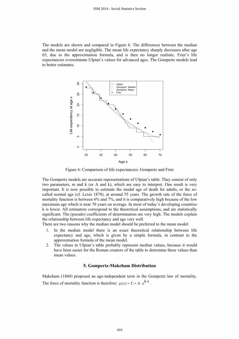
The models are shown and compared in Figure 6. The differences between the median and the mean model are negligible. The mean life expectancy sharply decreases after age 65, due to the approximation formula, and is then no longer realistic. Frier’s life expectancies overestimate Ulpian’s values for advanced ages. The Gompertz models lead to better estimates.

20 30 40 50 60 70

05

1015

2025

30

Age x

Life

exp

ecta

ncy

at a

ge x

UlpianGompertz: MedianGompertz: MeanFrier

Figure 6: Comparison of life expectancies: Gompertz and Frier

The Gompertz models are accurate representations of Ulpian’s table. They consist of only two parameters, m and k (or A and k), which are easy to interpret. One result is very important. It is now possible to estimate the modal age of death for adults, or the so-called normal age (cf. Lexis 1878), at around 55 years. The growth rate of the force of mortality function is between 6% and 7%, and it is comparatively high because of the low maximum age which is near 70 years on average. In most of today’s developing countries k is lower. All estimators correspond to the theoretical assumptions, and are statistically significant. The (pseudo) coefficients of determination are very high. The models explain the relationship between life expectancy and age very well. There are two reasons why the median model should be preferred to the mean model:

1. In the median model there is an exact theoretical relationship between life expectancy and age, which is given by a simple formula, in contrast to the approximation formula of the mean model.

2. The values in Ulpian’s table probably represent median values, because it would have been easier for the Roman creators of the table to determine these values than mean values.

5. Gompertz-Makeham Distribution

Makeham (1860) proposed an age-independent term in the Gompertz law of mortality. The force of mortality function is therefore: k x(x) C A e ⋅μ = + ⋅ .


416

The term C>0, which is independent of age, represents non-senescent deaths, such as deaths from accidents. The resulting survivorship function of the Gompertz-Makeham or Makeham model is:

A A k xl(x) exp e C xk k

⎛ ⎞⋅= − ⋅ − ⋅⎜ ⎟⎝ ⎠

with the modal value

k·(k - 4·C)) - 2·C + kln2 Ak

m

⎛ ⎞⎜ ⎟⎜ ⎟⋅⎝ ⎠= for k 4 C> ⋅ .

There is no explicit relationship between the median life expectancy and the age: ( )( )A exp k x e(x) C k e(x) A exp(k x) k ln 2 0⋅ ⋅ + + ⋅ ⋅ − ⋅ ⋅ − ⋅ = ,

but an inverse relationship can be deduced:

( )( )( )

k ln 2 C e(x)ln

A exp k e(x) 1x

k

⎛ ⎞⋅ − ⋅⎜ ⎟⎜ ⎟⋅ ⋅ −⎝ ⎠= .

We use this relationship in order to estimate the parameters of the model, where x is the regressand and e(x) is the regressor. The estimation results are given in Table 4. Solving the implicit function for x=20, 21, 22, ..70 yields a life expectancy function whose graph is shown in Figure 7. Table 4: Estimation results of the Gompertz-Makeham model (median) Dependant variable x=20, 21, ….70 Independant variable ( )e x Lower Upper Parameter Estimate Std Error 95% C.I. 95% C.I. A 2.85193E-04 2.0225E-04 -1.21453E-04 6.91839E-04 C 0.014106 3.3308E-03 7.40943E-03 0.020803 k 0.091553 0.010841 0.069757 0.113350 Convergence criterion met after 14 iterations. Residual SS (SSE) 280.08 Residual MS (MSE) 5.8349 Standard Deviation 2.4156 Degrees of Freedom 48 AICc 95.735 Pseudo R² 0.9747 Cases Included 51 Missing Cases 0 The parameter A is not statistically significant for the chosen level. Comparing some of the statistical properties of the Gompertz and the Makeham models is difficult or even impossible, because the Makeham model parameters were obtained by estimating an inverse function. The growth rate k must be higher, because of the age-independent term in the force of mortality function. The Gompertz and the Makeham function graphs do not differ very much. Makeham values are higher for middle age classes and lower for older age classes. Finally, we will compare the Makeham model using median life expectancies with the Makeham model using mean life expectancies. Mays (1971a,b) determined values for the Makeham constants through approximations and series expansions. The final values were obtained by Mays as follows (we use other symbols): A= 0.0000213685 , C= 0.01613025 , and k= ln(1.14536554) 0.1357238348= . With these values it is possible to calculate the mean and the modal life expectancy by numerical integration.


417

20 30 40 50 60 70

05

1015

2025

30

Age x

Life

exp

ecta

ncy

at a

ge x

UlpianGompertz: MedianMakeham: MedianFrier

Figure 7: Comparison of median life expectancies: Gompertz, Makeham, and Frier

The graphs of the median and the mean life expectancies are depicted in Figure 8. The mean values are slightly higher than the median values except for ages above 55. The Makeham mean model yields a modal value of about 62 years, whereas the Makeham median model yields a modal value of about 58 years. The Gompertz models and the Makeham models provide similar results if we look at the patterns of the functions. The main differences are the higher modal values. The values of the parameters in the Makeham mean model must be carefully interpreted, since the fit of Mays’ parameters is based on only three selected ages.

20 30 40 50 60 70

05

1015

2025

30

Age x

Life

exp

ecta

ncy

at a

ge x

UlpianMakeham: MeanMakeham: Median

Figure 8: Comparison of median and mean life expectancies (Makeham)

6. Conclusion

Our results show that we cannot definitively decide which is the best model, and we have only analyzed a limited number of models. We could use other models or change our


418

models by using varying sets of observations (e.g., ages from 30 to 70 and their corresponding life expectancies), or by varying our estimation procedures (e.g., it is possible to estimate the Gompertz parameters by linear least squares if one uses the logarithmic transformation of the force of mortality function). According to the principle of parsimony, which states that, among competing models and hypotheses, the model or hypothesis with the fewest assumptions or parameters should be selected, we chose the simple Gompertz median model for further analysis5.

References Abramowitz, M; Stegun, I A (1964): Handbook of mathematical functions, Washington, D.C. Achard M A (1902): Note sur le changement de taux dans le calcul des annuités viagères, Bulletin de

l’Institut des Actuaires Français, Vol 2. Ciecka, J E (2012): Ulpian’s table and the value of life annuities and usufructs, J. of Legal Econ., 19(1): 7-15. Coale, A J; Demeny, P (1966): Regional model life tables and stable populations, New York, NY. De Vries, T; Zwalve, W J (2004): Roman actuarial science and Ulpian’s life expectancy table, in: de Ligt, L;

Hemelrijk, E A; Singor, H W (eds): Roman rule and civic life: Local and regional perspectives, Amsterdam, 277-297.

Dupaquier J (1973): Sur une table (prétendument) florentine d’espérance de vie, Annales Économies, Sociétés, Civilisations, 28e année, No. 4, 1066-1070.

Forfar, D O (2004): Mortality Laws, Encyclopedia of Actuarial Science, Chichester. Frier, B W (1982): Roman life expectancy: Ulpian’s evidence, Harvard Studies in Classical Philology , 86:

213-51. Frier, B W (2000): Demography, in: Bowman, A K; Garnsey, P; Rathbone, D (eds): The Cambridge Ancient

History XI: The High Empire, A.D. 70–192, Second edition, Cambridge, 787-816. Gompertz, B (1825): On the nature of the function expressive of the law of human mortality, Philosophical Transactions of the Royal Society of London, Ser. A, 115, 513-585. Hildebrand, B (1866): Die amtliche Bevölkerungsstatistik im alten Rom, Jahrbücher für Nationalökonomie

und Statistik, 6: 81-96. Hopkins, K (1966): On the probable age structure of the Roman population, Populal. Studies, 20(2):245-264. Kohli, K (1975): Kommentar zur Dissertation von Niklaus Bernoulli: De Usu Artis Conjectandi in Jure, Die

Werke von Jakob Bernoulli, 3: 541-556. Kopf, E W (1926): The early history of the annuity, Proc. of the Casualty Actuarial Society, 13(27): 225-266. Langner, G (1998): Schätzung von Säuglingssterblichkeit und Lebenserwartung im Zeitalter des Imperium

Romanum, Methodenkritische Untersuchung, Historical Social Research, 23: 299-326. Lexis, W (1878): Sur la durée normale de la vie humaine et sur la théorie de la stabilité des rapports

statistiques, Annales de Démographie Internationale 2: 447-460. Makeham W M (1860): On the law of mortality and the construction of annuity tables, J. Inst. Actuaries and

Assur. Mag., 8: 301-310. Mays, W (1971a): Die Ulpian-Tafel, Blätter der DGVFM, 10(2): 271-292. Mays, W (1971b): Ulpian´s table, The Actuary, The Newsletter of the Society of Actuaries, 5(6). Müller A (1906): Ansätze zum Versicherungswesen in der römischen Kaiserzeit, Zeitschrift für die gesamte

Versicherungswissenschaft 2: 209-219. Parkin, T G (1992): Demography and Roman Society, Baltimore, Maryland. Pflaumer, P (2011): Methods for estimating selected life table parameters using the Gompertz distribution,

JSM Proceedings, Social Statistics Section. Alexandria, VA: American Statistical Association, 733-747. Pollard, J H (1991): Fun with Gompertz, Genus, XLVII-n.1-2, 1-20. Pollard, J (1998): An old tool – Modern applications, Actuarial Studies and Demography, Research Paper

No. 001/98, August. Sanchez-Moreno Ellart, C (2013): Ulpianic life table, The Encyclopedia of Ancient History, Edited by Bagnall, R S et al., New York, 6908-6910. Szilágyi, J (1963): Die Sterblichkeit in den Städten Mittel- und Süditaliens sowie Hispanien (in der

römischen Kaiserzeit), Acta Archaeologica Academiae Scientiarum Hungaricae 15: 129-224. Weiss, K (1973): Demographic models for anthropology, Washington, D.C., 1973. Woods, R (2007): Ancient and early modern mortality: Experience and understanding, The Economic

History Review, New Series, 60(2): 373-399. 5 The research will be continued in a paper, which is planned to be presented at the JSM 2015.


419

Documents

A Demometric Analysis of Ulpian´s Table