A DETERMINISTIC MODEL OF SCHISTOSOMIASIS WITH …milner/PDF/zhaomilner3.pdf · A DETERMINISTIC MODEL OF SCHISTOSOMIASIS WITH ... in tropical countries in Africa, ... A DETERMINISTIC

MATHEMATICAL BIOSCIENCES http://www.mbejournal.org/AND ENGINEERINGVolume 5, Number 3, July 2008 pp. 505–522

A DETERMINISTIC MODEL OF SCHISTOSOMIASIS WITHSPATIAL STRUCTURE

Fabio Augusto Milner

Department of Mathematics, Purdue University150 North University Street, West Lafayette, IN 47907-2067

Ruijun Zhao

Department of Mathematics, Purdue University150 North University Street, West Lafayette, IN 47907-2067

(Communicated by Stephen Gourley)

Abstract. It has been observed in several settings that schistosomiasis is lessprevalent in segments of river with fast current than in those with slow current.Some believe that this can be attributed to flush-away of intermediate hostsnails. However, free-swimming parasite larvae are very active in searching forsuitable hosts, which indicates that the flush-away of larvae may also be veryimportant. In this paper, the authors establish a model with spatial structurethat characterizes the density change of parasites following the flush-away oflarvae. It is shown that the reproductive number, which is an indicator ofprevalence of parasitism, is a decreasing function of the river current velocity.Moreover, numerical simulations suggest that the mean parasite load is lowwhen the velocity of river current flow is sufficiently high.

1. Introduction. Schistosomiasis, a parasite (schistosome)-induced disease, is alsoknown as bilharzia after Theodor Bilharz, who first identified the parasite in Egyptin 1851. Infection is widespread with a relatively low mortality rate but a highmorbidity rate, causing severe debilitating illness. The disease is generally associ-ated with rural poverty. An estimated 170 million people suffered it in sub-SaharanAfrica in 2004, and so did a further 30 million in North Africa, Asia, and SouthAmerica [26].

Schistosomes have to go through an intermediate host (snails in most cases)to complete their life cycle: from eggs, to miracidia, to cercariae, finally to adultflukes. Unlike direct parasites, schistosomes have two stages of reproduction - sexualproduction in humans and asexual amplification in snails. Mathematical modelingand analysis of schistosomiasis has drawn the attention of many researchers sincethe first paper by Macdonald in 1965 [15]. Thereafter, Anderson and May [2,3], Cohen [6], Nasell [16], Dobson [7], Adler and Kretzschmar [1], Pugliese [17],and many other researchers built excellent unstructured models and developed adecent understanding of transmission mechanism of schistosomiasis. However, manyimportant biological facts (e.g., age/size- or spatial factors) are overlooked in thesemodels. For example, snails tend to cease production eventually, and they quickly

2000 Mathematics Subject Classification. Primary: 92D30, 92D40; Secondary: 93C15, 93C20.Key words and phrases. schistosomiasis, reproductive numbers, delay differential equations.The first author is supported in part by NSF grant DMS-0314575.

505

506 FABIO AUGUSTO MILNER AND RUIJUN ZHAO

die after infection [12, 20]; children of school age usually exhibit higher prevalenceof schistosome infections than other groups [5, 24]; there are fewer incidences ofinfections reported by adventurers who traveled to northern parts of Omo River(faster flow) than by those to southern parts (slower flow) [19]. Recently, someage-structured models were proposed [9, 24] and optimal control strategies werediscussed. However, there is no mathematical model of schistosomiasis with spatialstructure.

In this paper, we focus on how the speed of a river affects the transmission dy-namics of schistosomiasis by assuming flush-away of only free-swimming miracidiaand cercariae, and nothing else. In the literature, lower incidences of schistosomiasisalong a river with higher speed occur with fewer snails in the aquatic environment[23]. Utzinger et al. believed that Biomphalaria pfeifferi have preference for acertain range of river current velocity, and they claimed a paucity of snails as areason for low incidences [23]. Moreover, spatial microhabitat selection by B. pfeif-feri also depends on the water depth [23]. On the other hand, when infected snailsare prevalent, environmentally triggered downward swimming can quickly bring lar-vae (planktonic cercariae) to the bed, promoting contact with benthic intermediatehosts [11]. Compared with snails, miracidia and cercariae spend most of their lifein search for hosts and move along with water flow. Thus, the flush-away of par-asite larvae plays an important role in the host-parasite system. Furthermore, westudy a control strategy related to treatment and prevention of infected humansand estimate a minimal effort to eradicate the disease.

The present paper is structured as follows: in the next section, a mathematicalmodel with spatial structure is given; in Section 3, its well-posedness is established;in Section 4, a reduced model (ODE model, spatially uniform) is studied analyti-cally and numerically; in Section 5, the full model is analyzed and simulations areprovided; finally, we present some discussion and conclusions.

2. A mathematical model with spatial structure. Schistosomiasis is foundin tropical countries in Africa, the Caribbean, eastern South America, east Asia,and in the Middle East. It is prevalent in villages near rivers or lakes. Since thepurpose of our paper is to study the influence of river velocity on the transmissiondynamics of schistosomiasis, we assume the aquatic habitat to be a river, whichhas a geometry of line segment [0, L]. Moreover, we assume that the origin of theriver (x = 0) is free of parasites, and humans can have an active impact only on acompact region [0, L].

In the following, we make assumptions as in [25].(H0) Human beings and snails grow logistically in the absence of parasites with

corresponding carrying capacities.(H1) The rate of parasite-induced human mortality is linearly proportional to the

number of parasites a person harbors.(H2) Infected snails do not reproduce and have high potential mortality.(H3) Distribution of parasites among human beings is overdispersed.(H4) Birth rates of hosts are greater than their death rates, bj − µj0 > 0, j = h, s.(H5) Productivity of cercariae by each infected snail is independent of the dose of

miracidia exposed.The biological justification and mathematical methodology can be seen in [2,

3, 12, 14, 20, 21, 22]. We further assume that only miracidia and cercariae arespatially dependent. Human beings are active everywhere in the habitat, so that

A DETERMINISTIC MODEL OF SCHISTOSOMIASIS WITH SPATIAL STRUCTURE 507

their contribution to the environment can be treated as homogeneous. The same istrue for parasites, because they reside inside the human body. We further assumesnails are more or less uniformly distributed along the river, because they live inthe river bed.

Miracidia and cercariae swim in the river with certain directional preference,such as towards to light [11], and toward intermediate host snails. In this paper, weneglect all these motions and assume that the larvae are flushed away by the riverflow. In fact, a cercaria can swim up to 5 meters per day, and a miracidium canswim up to 50 meters per day [13]. The speed of larvae swimming is at least a 3-order magnitude less than a typical river velocity. It can be ignored. For simplicity,the river velocity is assumed to be a positive constant.

Let H(t), P (t), S(t), I(t) denote the total numbers of human beings, adult par-asites, uninfected snails and infected snails at time t, respectively. Let m(x, t),c(x, t) denote the density of free-living miracidia, free-living cercariae at time t and

location x, respectively. Let C(t) =∫ L

0

c(x, t)dx, M(t) =∫ L

0

m(x, t)dx denote the

total numbers of miracidia and cercariae at time t, respectively. All demographicand epidemiological parameters are listed in Table 1, and most of them are identifiedin [8, 25].

Table 1. Parameter definitions

Parameter Definitionbh per capita birth rate of human beingsµh0 per capita natural death rate of human beingsµh1 extra per capita death rate of human beings due to overcrowdingLh carrying capacity of environment for human beingsα parasite-induced death rate of human beings per parasiteβ production rate of cercariae per infected snailλ attachment rate of cercariae to human beingsκ “clumping parameter” of binomial distribution of adult parasitesµp per capita death rate of parasitesr treatment-induced rate of parasitesbs per capita birth rate of snailsµs0 per capita natural death rate of snailsµs1 additional per capita death rate of snails due to overcrowdingLs carrying capacity of environment for snailsρ contact rate (per snail) of uninfected snails with miracidiads parasite-induced death rate of snailsbp mean number of eggs (miracidia) laid per parasiteζ “efficacy” of cercariae in infecting humans (0 ≤ ζ ≤ 1)µm per capita death rate of miracidiaµc per capita death rate of cercariaev river current velocity


A mathematical model of schistosomiasis with spatial concerns consists of thefollowing system of differential equations:

dH

dt= (bh − µh0 − µh1H)H − αP,

dP

dt= ζHC − α(κ+1

κ )(

P 2

H

)− (µh0 + µh1H + µp + α + r)P,

dS

dt= (bs − µs0 − µs1(S + I))S − ρMS,

dI

dt= ρMS − (µs0 + µs1(S + I) + ds)I,

∂m

∂t= −v

∂m

∂x+ bpP − µmm,

∂c

∂t= −v

∂c

∂x+ βI − µcc,

(1)

along with homogeneous Dirichlet boundary conditions on the inflow boundary forthe two partial differential equations

m(0, t) = 0, c(0, t) = 0, (2)

and nonnegative initial distributions

H(0) = H0, P (0) = P0, S(0) = S0, I(0) = I0,m(x, 0) = m0(x), c(x, 0) = c0(x). (3)

Remark 1. System (1) is not self-consistent in that the loss of miracidia andcercariae penetrating into hosts is not reflected in the change of densities of thesetwo larvae. In fact, free-living miracidia and cercariae live at most 48 hours in freshwater, and they lose ability to penetrate into hosts after first several hours when theyare active in searching hosts [13]. On the other hand, this special treatment allowsus to reduce the six-dimensional System (1) to a four-dimensional delay differentialequations after explicitly solving the two hyperbolic equations.

Remark 2. Boundary conditions (2) can be modified into some nonnegative func-tions, in which the model can be applied to study how a contaminated river byschistosomiasis can affect its downstream regions.

3. Well-posedness. To determine the well-posedness of System (1), we reduce itto an equivalent lower-order dimensional system.

Since equations (1.v) and (1.vi) are first-order hyperbolic equations, we can solvethem exactly along characteristic lines x = τ + vt, where τ is a parameter. Denotem(t) = m(τ + vt, t). Then equation (1.v) becomes

dm

dt+ µmm = bpP. (4)

Since the habitat has finite length L, we can group characteristic lines as above x =vt and below x = vt. The solution of equation (4) in the region {(x, t)|vt < x < L}is

m(t) = e−µmtm(0) + bp

∫ t

0

e−µm(t−s)P (s)ds, (5)


and the solution of equation (4) in the region {(x, t)|0 < x < vt} is

m(t) = e−µmx

v m(t− x

v) + bp

∫ t

xv

e−µm(t−s)P (s)ds. (6)

Thus the solution of equation (1.v) is

m(x, t) =

e−µmtm0(x− vt) + bp

∫ t

0

e−µm(t−s)P (s)ds if x > vt,

bp

∫ xv

0

e−µmsP (t− s)ds if x ≤ vt.

(7)

The total number of miracidia at time t can be obtained by integrating equation(7) from x = 0 to x = L,

M(t) =

bp

∫ vt

0

∫ xv

0

e−µmsP (t− s)dsdx if t <L

v,

+∫ L

vt

[e−µmtm0(x− vt) + bp

∫ t

0

e−µm(t−s)P (s)ds

]dx

bp

∫ L

0

∫ xv

0

e−µmsP (t− s)dsdx if t ≥ L

v.

(8)

Similarly, the solution of equation (1.vi) is

c(x, t) =

e−µctc0(x− vt) + β

∫ t

0

e−µc(t−s)I(s)ds if x > vt,

β

∫ xv

0

e−µcsI(t− s)ds if x ≤ vt,

(9)

and total number of cercariae at time t is

C(t) =

β

∫ vt

0

∫ xv

0

e−µcsI(t− s)dsdx if t < Lv ,

+∫ L

vt

[e−µctc0(x− vt) + β

∫ t

0

e−µc(t−s)I(s)ds

]dx

β

∫ L

0

∫ xv

0

e−µcsI(t− s)dsdx if t ≥ Lv .

(10)

As in [25], we investigate an equivalent system by introducing two new unknowns:mean parasite load per person R = P/H and total number of snail populationT = S+I. Substituting equation (8) and equation (10) into System (1) and carryingout some calculation and simplification, we have the following delay differential


equations:

dH

dt= (bh − µh0 − µh1H)H − αRH,

dR

dt= ζC(S(·), T (·))− α

κR2 − (bh + µp + α + r)R,

dS

dt= (bs − µs0 − µs1T )S − ρM(H(·), R(·))S,

dT

dt= (bs − µs0 − µs1T )T − (bs + ds)(T − S),

(11)

where M(H(·), R(·)) and C(S(·), T (·)) have the same expressions as in (8) and (10)except replacing P and I by HR and T − S, respectively.

Lemma 3.1. If H(0), R(0), and S(0) are positive and T (0) > S(0), then solutionsof Eqs. (11) are positive, and T (t) > S(t) as long as they exists.

Proof. Equation (11.i) and equation (11.iii) imply that H and S are nonnegative ifthe initial data are nonnegative. Subtracting equation (11.iii) from equation (11.iv),then

d(T − S)dt

= (bs − µs0 − µs1T )(T − S)− (bs + ds)(T − S) + ρM(H(·), R(·)). (12)

It is clear from equation (8) that ∀t > 0; if R(s), 0 < s < t is nonnegative, then M(t)is nonnegative. equation (12) implies that if M(t) is nonnegative, then (T −S)(t) isnonnegative. Moreover, from equation (10), if (T − S)(s), 0 < s < t is nonnegative,then C(t) is nonnegative, and equation (11.ii) implies R(t) is nonnegative.

Therefore, when H(0) > 0 and S(0) > 0, if either R(0) > 0 or T (0) > S(0),then for small ε > 0 we certainly have H,R, S,M, C and T − S positive on (0, ε).It is clear that equation (11.i) gives the positivity of H, equation (11.iii) gives thepositivity of S, and then equation (11.iv) gives the positivity of T as long as theyexist. Hence, it suffices to show that T −S must remain positive as long as it exists,since that is sufficient (in fact, equivalent) to establish the positivity of R.

Suppose that T−S vanishes for some positive time, and let t be the smallest suchtime. Then, T−S is positive on [0, t) and T (t) = S(t). It follows that C(t) > 0 fromequation (10). Then, R is positive on [0, t] from equation (11.ii) and then equation(12) implies that T − S is positive on [0, t], contradicting T (t) = S(t). Thus T − Sremains positive as long as it exists, and so do R, M and C. Moreover, m(x, t) andc(x, t) are also positive if R(t),H(t), T (t) − S(t) are positive. This completes thepositivity of the solution to System (11).

Lemma 3.2. If H(0), R(0), and S(0) are positive and T (0) > S(0), then solutionsof equation (11) H(t), R(t), S(t) and T (t) are uniformly bounded as long as theyexist.


Proof. For convenience, we introduce three new notations:

δ = bh + µp + α + r,

ξ = L +v

µc(e−

µcv L − 1),

η = L +v

µm(e−

µmv L − 1).

(13)

It is evident that equation (11.i) and equation (11.iv) imply that H ≤ Lh andT ≤ Ls. Moreover, S ≤ Ls and I ≤ Ls.

For the boundedness of C(t), it suffices to check for t > L/v,

C(t) = β

∫ L

0

∫ xv

0

e−µcs(T (t− s)− S(t− s))dsdx

≤ βLs

µc

∫ L

0

(1− e−µcxv )dx

=βξLs

µc.

(14)

From equation (11.ii), we have an estimationdR

dt= ζC(S(·), T (·))− α

κR2 − δR ≤ ζβξLs

µc− δR.

The boundedness of R follows immediately

R ≤ R0e−δt +

ζβξLs

µc(1− e−δt) ≤ R0 +

ζβξLs

µc. (15)

Similarly, it suffices to check the boundedness of M(t) for t > ÃL/v,

M(t) = bp

∫ L

0

∫ xv

0

e−µmsR(t− s)H(t− s))dsdx

≤ bpηLh

µm

[R0 +

ζβξLs

µc

].

(16)

Concerning the existence and uniqueness of solution of the problem, we consultsome results by Driver in [4]. Consider a system of Volterra functional differentialequations

x′(t) = F(t,x(·)), t ≤ t0, (17)in which x = (x1, . . . , xn), F = (f1, . . . , fn) and x′i(t) = fi(t, x1(s), . . . , xn(s); α ≤s ≤ t) for t ≤ t0, α ≤ −∞, α ≤ t0, and i = 1, . . . , n.

Lemma 3.3. (Driver (1962)) Let F(t,x(·) be continuous in t and locally Lipschitzin x and let φ ∈ C([α, t0] → D). Then there exists an h > 0 such that a uniquesolution x(t) = x(t, t0, φ) exists for α ≤ t ≤ t0 + h.

Rewriting System (11) into a form of equation (17), it is easy to show thatF(t,x) is locally Lipschitz in x and is independent of t by observing equation (10),equation (8) and System (11). The local existence and uniqueness of solutions canbe obtained by Lemma 3.3. The global existence and uniqueness of solutions is


guaranteed by the uniform boundedness. Then, the following theorem has beenproved.

Theorem 3.4. System (1), or equivalently, System (11) admits a unique solutionfor all time. Moreover, if H(0) and S(0) are positive and either T (0) > S(0), orM(0) > 0, or R(0) > 0, or C(0) > 0, then H,R, S, m and c are positive and T > Sas long as they exist.

Remark 3. It is worthy to point out that the domain of φ is {0} for t ≤ Lv and

[0, Lv ] for t > L

v when we apply Lemma 3.3 to prove Theorem 3.4.

4. Special case: Model in spatially uniform distribution. At first glance,it seems strange to talk about a case where all species are uniformly distributedin space, since the homogeneous in-flow boundary conditions for miracidia andcercariae will force a disease-free solution. However, spatially uniform distributioncan happen at steady states if nonhomogeneous in-flow boundary conditions areimposed.

Instead of looking at System (1), we study an equivalent system in which theunknowns are H, R, S, T, m and c,

dH


dR

dt= ζLc− α

κR2 − (bh + µp + α + r)R,

dS

dt= (bs − µs0 − µs1(S + I))S − ρLmS,

dT

dt= (bs − µs0 − µs1T )T − (bs + ds)(T − S),

dm

dt= bpP − µmm,

dc

dt= βI − µcc.

(18)

It is clear that System (18) admits four parasite-free steady states:

E0 = (H0, R0, S0, T0,m0, c0) = (0, 0, 0, 0,0,0),E1 = (H1, R1, S1, T1,m1, c1) = (0, 0, Ls, Ls,0,0),E2 = (H2, R2, S2, T2,m2, c2) = (Lh, 0, 0, 0,0,0),EDFE = (HDFE , RDFE , SDFE , TDFE ,mDFE , cDFE) = (Lh, 0, Ls, Ls,0,0).

where, EDFE represents (H, P, S, I, m, c) = (Lh, 0, Ls, 0,0,0) for System (1). E0

is the trivial equilibrium, while E1 and E2 are semitrivial in that they represent,respectively, the ultimate state of a logistic population of snails and of humans inthe absence of parasitism.

Carrying out the similar calculations as in [25], at steady states of System (18),H satisfies a cubic equation

H3 + a2H2 + a1H + a0 = 0, (19)


where

a2 = −Lh,

a1 =αµm(bs − µs0)

ρbpLµh1+

αµs1µcµ2m(bs + ds)

κζβρ2b2pL

3,

a0 = −αµs1µcµ2m(bh − µh0)(bs + ds)

κζβµh1ρ2b2pL

3− (bh + µp + α + r)αµs1µcµ

2m(bs + ds)

ζβµh1ρ2b2pL

3,

Define

Q =3a1 − a2

2

9, U =

9a1a2 − 27a0 − 2a32

54, D = Q3 + R2. (20)

Theorem 4.1. Let D, Q and U be defined in equation (20), and consider D andU as functions of treatment rate r.

• If Q > 0 or if Q < 0, U(0) > 0 and D(0) > 0, then equation (19) admits onlyone positive root;

• If Q < 0, and if D(0) < 0, then equation (19) admits three, then two, andfinally one positive root as r increases.

• If Q < 0, U(0) < 0 and D(0) > 0, then equation (19) admits one, two, thenthree, two, and finally one positive root as r increases.

Remark 4. It can be easily seen from System (18) that if a root H∗ of equa-

tion (19) satisfies 0 < H∗ < Lh and rs >ρbpL(bh − µh0)

αµm(1 − H∗

Lh)H∗ (or rs >

ρbpLLh(bh − µh0)4αµm

), then System (18) has an interior equilibrium with human pop-

ulation size H∗.

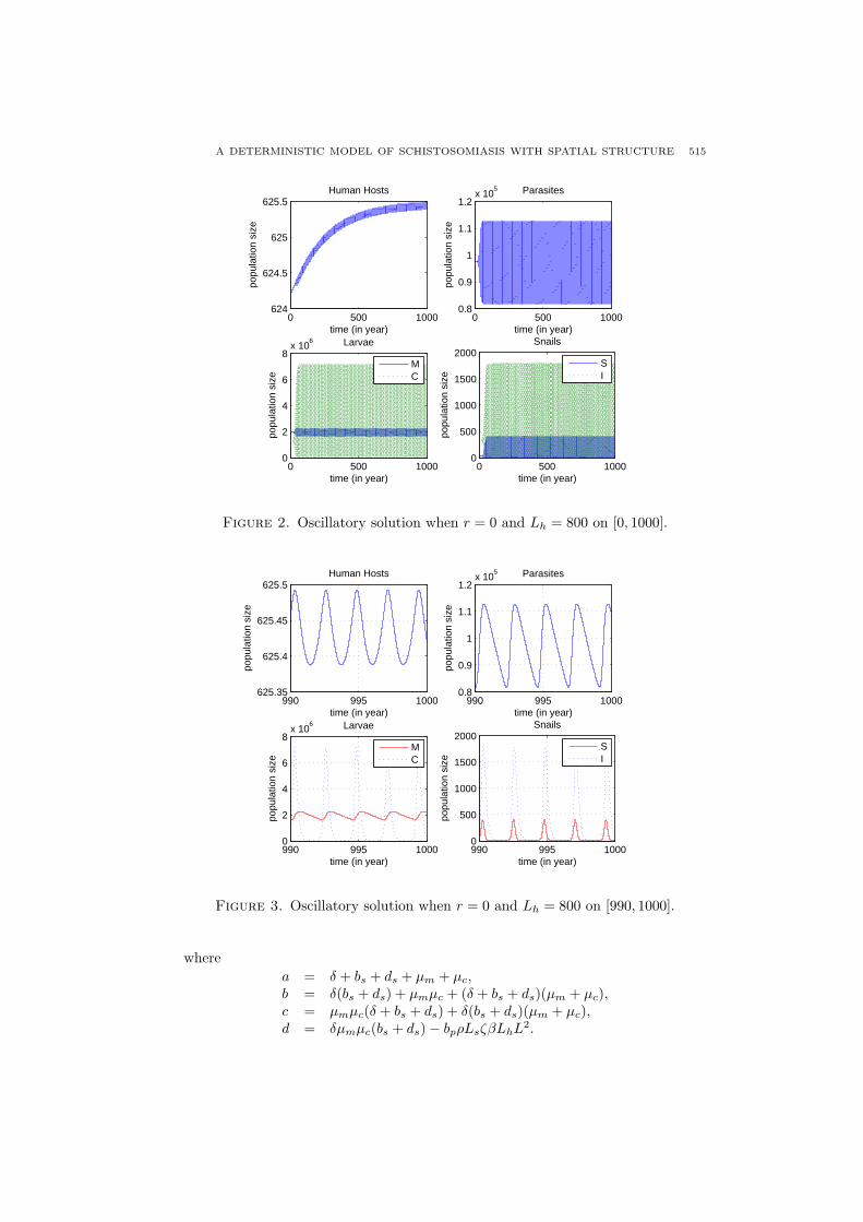
As pointed out in [25], it is hopeless to do an analytical stability analysis andso we run some numerical simulations and generate a bifurcation diagram with twoparameters Lh and r while the rest are fixed. Figure 1 shows a bifurcation diagram,where the parameters are chosen as L = 1, µh0 = 1/70, bh = 3/140, α = 0.00001,ζ = 0.000027, κ = 0.243, µp = 0.2, µs0 = 0.5, bs = 80, Ls = 20000, ρ = 0.00004,ds = 6.0, µm = 180, µc = 180, β = 4000µc, bp = 20µm. Figure 2 and Figure 3show an oscillatory solution when parameters are in the region V, and simulationsare done under r = 0 and Lh = 800.

By analyzing the Jacobian matrices of System (18) at E0, E1, E2, we can obtainsimilar results as in [25].

Theorem 4.2. E0, E1 and E2 are unstable.

Define a reproductive number for parasitism

R∗0 =ζβρbpLhLsL

2

µmµc(bs + ds)(bh + µp + α + r). (21)

Theorem 4.3. If R∗0 < 1, then EDFE is locally asymptotically stable; if R∗0 > 1then EDFE is unstable.


0 0.2 0.4 0.6 0.8 1 1.2 1.40

200

400

600

800

1000

1200Bifurcation Diagram

Treatment rate, r

Car

ryin

g ca

paci

ty fo

r hu

man

bei

ngs

L h

V

IV

II

III

VI

I

Figure 1. Bifurcation Diagram. In region I, there is no interiorequilibrium and EDFE is globally asymptotically stable. In regionII, there is one interior equilibrium, of which H∗ corresponds to thesmallest root of equation (19) in terms of magnitude, and it is glob-ally asymptotically stable. In region III, there is also one globallyasymptotically stable interior equilibrium, of which H∗ correspondsto the largest root. In region IV, there are three interior equilibria,of which the largest and the smallest roots are locally asymptoti-cally stable. In region V, there are also three interior equilibria, ofwhich two largest are unstable so that oscillatory solutions occur.In region VI, there is only one interior equilibrium but unstable, sooscillatory solutions exist.

Proof. The Jacobian of System (1) in spatially uniform distribution at the equilib-rium EDFE is

J1(EDFE) =

−(bh − µh0) −α 0 0 0 00 −δ 0 0 0 ζLLh

0 0 −(bs − µs0) −(bs − µs0) −ρLLs 00 0 0 −(bs + ds) ρLLs 00 bp 0 0 −µm 00 0 0 β 0 −µc

.

The characteristic polynomial of J1(EDFE) is

f(λ) = (λ + (bh − µh0))(λ + (bs − µs0))[(λ + δ)(λ + bs + ds)(λ + µm)(λ + µc)− bpρLsζβLhL2]. (22)

It is clear that λ = −(bh−µh0) and λ = −(bs−µs0) are two roots of f(λ) and theyare negative from our assumptions. Whether f(λ) has positive roots is determinedby the forth order factor

f1(λ) = (λ + δ)(λ + bs + ds)(λ + µm)(λ + µc)− bpρLsζβLhL2

= λ4 + aλ3 + bλ2 + cλ + d,(23)


0 500 1000624

624.5

625

625.5

time (in year)

popu

latio

n si

ze

Human Hosts

0 500 10000.8

0.9

1

1.1

1.2x 10

5 Parasites

time (in year)

popu

latio

n si

ze

0 500 10000

2

4

6

8x 10

6

time (in year)

popu

latio

n si

ze

Larvae

MC

0 500 10000

500

1000

1500

2000

time (in year)

popu

latio

n si

ze

Snails

SI

Figure 2. Oscillatory solution when r = 0 and Lh = 800 on [0, 1000].

990 995 1000625.35

625.4

625.45

625.5

time (in year)

popu

latio

n si

ze

Human Hosts

990 995 10000.8

0.9

1

1.1

1.2x 10

5

time (in year)

popu

latio

n si

ze

Parasites

990 995 10000

2

4

6

8x 10

6

time (in year)

popu

latio

n si

ze

Larvae

MC

990 995 10000

500

1000

1500

2000

time (in year)

popu

latio

n si

ze

Snails

SI

Figure 3. Oscillatory solution when r = 0 and Lh = 800 on [990, 1000].

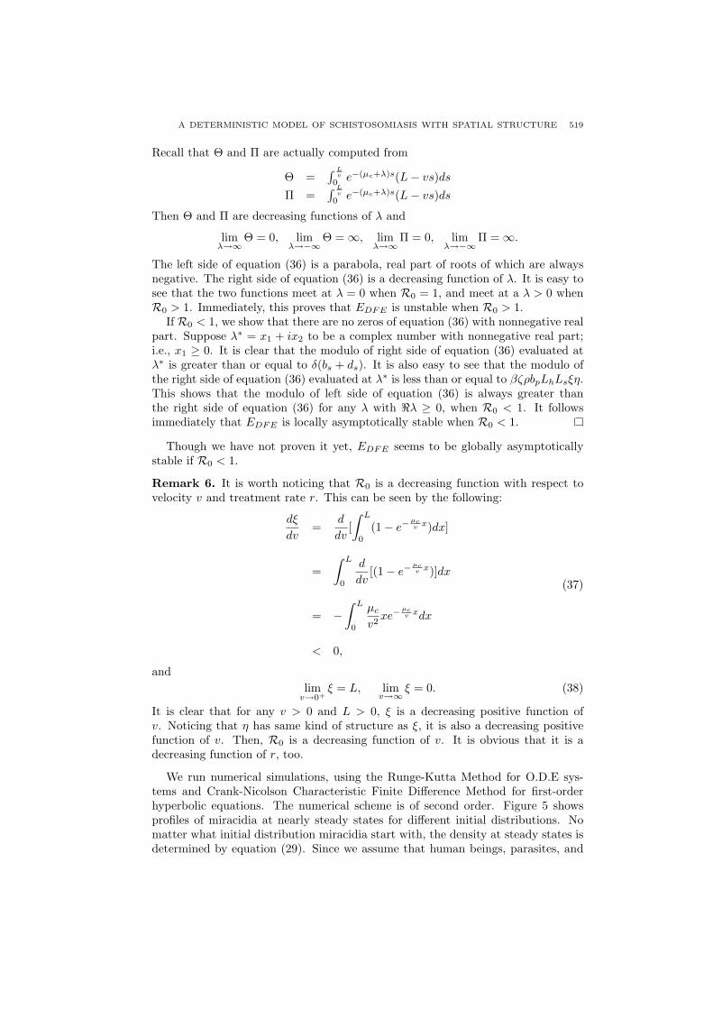
wherea = δ + bs + ds + µm + µc,b = δ(bs + ds) + µmµc + (δ + bs + ds)(µm + µc),c = µmµc(δ + bs + ds) + δ(bs + ds)(µm + µc),d = δµmµc(bs + ds)− bpρLsζβLhL2.


Following a theorem we owe to Strelitz (1977), the polynomial f1(λ) is stable ifand only if a > 0, b > 0, 0 < c < ab, 0 < d < (abc − c2)/a2. Note it is clear thata > 0, b > 0, c > 0. If R∗0 < 1 (which implies d < 0), then EDFE is unstable. IfR∗0 > 1, then d > 0, we have to check the other restrictions to test whether f1(λ)is stable or not.Carrying out multiplications and simplifications, it is clear that

ab− c = [δ(bs + ds)(δ + bs + ds) + (µm + µc)(δ + bs + ds)2

+µmµc(µm + µc) + (δ + bs + ds)(µm + µc)2

> 0.(24)

Moreover notice that

abc− c2 = c(ab− c)= δµmµc(bs + ds)(δ + bs + ds)2 + (δ + bs + ds)(µm + µc)δ2(bs + ds)2

+µmµc(µm + µc)(δ + bs + ds)3 + δ(bs + ds)(µm + µc)2(δ + bs + ds)2

+(µm + µc)(δ + bs + ds)µ2mµ2

c + δµmµc(bs + ds)(µm + µc)2

+µmµc(µm + µc)2(δ + bs + ds)2

+δ(bs + ds)(δ + bs + ds)(µm + µc)3,(25)

a2d = (δ + bs + ds + µm + µc)2[δµmµc(bs + ds)− bpρLsζβLhL2]+2δµmµc(bs + ds)(µm + µc)(δ + bs + ds)−bpρLsζβLhL2(δ + bs + ds + µm + µc)2.

(26)

Thus,

abc− c2 − a2d= (abc− c2)− a2d≥ (µm + µc)(δ + bs + ds)δ2(bs + ds)2 + δ(bs + ds)(δ + bs + ds)2(µm + µc)2

+(µm + µc)(δ + bs + ds)µ2mµ2

c + µmµc(µm + µc)2(δ + bs + ds)2

+(µm + µc)(δ + bs + ds)[µmµc(δ + bs + ds)2 + δ(bs + ds)(µ2m + µ2

c)]> 0.

(27)If R∗0 < 1, the characteristic polynomial f1(λ) is stable by Strelitz, and so is f(λ).Then, EDFE is locally asymptotical stable.

Remark 5. We conjecture that EDFE is actually a globally asymptotical steadystate if R∗0 < 1. Numerical simulations verified that the reproductive number isindeed a threshold for the system. As shown in Figure 4, if R∗0 > 1, the parasitismpersists, but if R∗0 < 1, then parasitism disappears.

5. Model with spatial structure. In Section 3, we established the existence anduniqueness of solution of System (11). In this section we focus on some stabilityand bifurcation analysis.

From System (1), at steady states, m satisfies

−vdm

dx+ bpP − µmm = 0, (28)

together with in-flow boundary condition

m(0) = 0.


0 500 1000 15000.02

0.025

0.03

0.035

0.04

0.045

0.05

0.055

0.06

0.065

0.07

time (in year)

aver

age

load

Mean Parasite Load / Person

0 5 10 15 200

5

10

15

time (in year)

aver

age

load

Mean Parasite Load / Person

Figure 4. Mean parasite load per person for different reproductivenumber R∗0. On the left graph, R∗0 = 1.000622; on the right graph,R∗0 = 0.999378, where Lh = 800, and r are chosen to match R∗0.

It is not hard to solve m explicitly as

m(x) =bpP

µm(1− e−

µmv x). (29)

Similarly, at steady states, c can be solved as

c(x) =βI

µc(1− e−

µcv x). (30)

Thus M =∫ L

0m(x)dx and C =

∫ L

0c(x)dx are given by

M =bpη

µmP, C =

βξ

µcI, (31)

where ξ and η are defined in equation (13).As shown in previous section, the existence of interior equilibria of System (1)

can be established as in Theorem 4.1. Moreover, an analytical stability analysis atthese interior equilibria is almost impossible. We turn our attention to the disease-free equilibria of System (11). Allow us to abuse notations: let E0, E1, E1, EDFE

again represent the disease free equilibria of System (11), where

E0 = (H0, R0, S0, T0) = (0, 0, 0, 0),E1 = (H1, R1, S1, T11) = (0, 0, Ls, Ls),E2 = (H2, R2, S2, T2) = (Lh, 0, 0, 0),EDFE = (HDFE , RDFE , SDFE , TDFE) = (Lh, 0, Ls, Ls).


Theorem 5.1. E0, E1 and E2 are unstable.

Proof. The linearization of (11) at an equilibrium (H∗, R∗, S∗, T∗) gives the followingcharacteristic equation:

det

a11 −αH∗ 0 00 a22 −ζβΠ ζβΠ

−ρbpΘR∗S∗ −ρbpΘH∗S∗ a33 −µs1S∗0 0 bs + ds a44

= 0. (32)

whereΘ = L

µm+λ + v(µm+λ)2 (e−

(µm+λ)Lv − 1),

Π = Lµc+λ + v

(µc+λ)2 (e−(µc+λ)L

v − 1),a11 = −λ + (bh − µh0)− 2µh1H∗ − αR∗,a22 = −λ− 2α

κ R∗ − δ,a33 = −λ + (bs + µs0)− µs1T∗ − ρbpηH∗R∗,a44 = −λ + (bs − µs0)− 2µs1T∗ − (bs + ds)

The characteristic polynomial (32) has positive roots at E0, E1 and E2 under ourassumptions; then we prove the conclusion.

Define the reproductive number for System (1) as

R0 =ζβρbpLhLsξη

µcµm(bs + ds)(bh + µp + α + r). (33)

Theorem 5.2. If R0 < 1, then EDFE is locally asymptotically stable; if R0 > 1then EDFE is unstable.

Proof. It turns out that it is easier to analyze an equivalent delay differential equa-tions of System (11) as follows

dH


dP

dt= ζHC(I(·))− α(κ+1

κ )(

P 2

H

)− (µh0 + µh1H + µp + α + r)P,

dS

dt= (bs − µs0 − µs1(S + I))S − ρM(P (·))S,

dI

dt= ρM(P (·))S − (µs0 + µs1(S + I) + ds)I.

(34)

The linearization of (34) at an equilibrium EDEF gives the following characteristicequation:

det

−λ− (bh − µh0) −α 0 00 −λ− δ 0 βζLhΠ0 −ρbpLsΘ −λ− (bs − µs0) −(bs − µs0)0 ρbpLsΘ 0 −λ− (bs + ds)

= 0.

(35)It is clear (for instance, by exchanging second and third rows and columns) thatλ1 = −(bh − µh0) and λ2 = −(bs − µs0) are two zeros of (35), and other zeros of(35) are determined by

λ2 + (δ + bs + ds)λ + δ(bs + ds) = βζρbpLhLsΘΠ. (36)


Recall that Θ and Π are actually computed from

Θ =∫ L

v

0e−(µc+λ)s(L− vs)ds

Π =∫ L

v

0e−(µc+λ)s(L− vs)ds

Then Θ and Π are decreasing functions of λ and

limλ→∞

Θ = 0, limλ→−∞

Θ = ∞, limλ→∞

Π = 0, limλ→−∞

Π = ∞.

The left side of equation (36) is a parabola, real part of roots of which are alwaysnegative. The right side of equation (36) is a decreasing function of λ. It is easy tosee that the two functions meet at λ = 0 when R0 = 1, and meet at a λ > 0 whenR0 > 1. Immediately, this proves that EDFE is unstable when R0 > 1.

If R0 < 1, we show that there are no zeros of equation (36) with nonnegative realpart. Suppose λ∗ = x1 + ix2 to be a complex number with nonnegative real part;i.e., x1 ≥ 0. It is clear that the modulo of right side of equation (36) evaluated atλ∗ is greater than or equal to δ(bs + ds). It is also easy to see that the modulo ofthe right side of equation (36) evaluated at λ∗ is less than or equal to βζρbpLhLsξη.This shows that the modulo of left side of equation (36) is always greater thanthe right side of equation (36) for any λ with <λ ≥ 0, when R0 < 1. It followsimmediately that EDFE is locally asymptotically stable when R0 < 1.

Though we have not proven it yet, EDFE seems to be globally asymptoticallystable if R0 < 1.

Remark 6. It is worth noticing that R0 is a decreasing function with respect tovelocity v and treatment rate r. This can be seen by the following:

dξ

dv=

d

dv[∫ L

0

(1− e−µcv x)dx]

=∫ L

0

d

dv[(1− e−

µcv x)]dx

= −∫ L

0

µc

v2xe−

µcv xdx

< 0,

(37)

andlim

v→0+ξ = L, lim

v→∞ξ = 0. (38)

It is clear that for any v > 0 and L > 0, ξ is a decreasing positive function ofv. Noticing that η has same kind of structure as ξ, it is also a decreasing positivefunction of v. Then, R0 is a decreasing function of v. It is obvious that it is adecreasing function of r, too.

We run numerical simulations, using the Runge-Kutta Method for O.D.E sys-tems and Crank-Nicolson Characteristic Finite Difference Method for first-orderhyperbolic equations. The numerical scheme is of second order. Figure 5 showsprofiles of miracidia at nearly steady states for different initial distributions. Nomatter what initial distribution miracidia start with, the density at steady states isdetermined by equation (29). Since we assume that human beings, parasites, and


00.5

11.5

2

0

0.5

10

2

4

6

8

10

12

x 105

time t

Miracidia

space x

dens

ity m

(x,t)

00.5

11.5

2

0

0.5

10

2

4

6

8

10

12

x 105

time t

Miracidia

space x

dens

ity m

(x,t)

Figure 5. Density plots of miracidia: on the top graph, miracidiastart with a sine function; on the bottom graph, miracidia startwith a cubic function. Parameters are chosen as Lh = 800, v = 1,and the rest are same as in Section 3, except µm = 1, µc = 1.

snails are spatially independent, the profiles of cercariae at steady states should besimilar to those of miracidia.

6. Discussions and conclusions. Endemic schistosomiasis is usually associatedwith a large human population and relatively slow river flow [19]. A large number ofhuman beings provides a big reservoir for destination hosts, and by contaminatingthe nearby aquatic environment, the residents create a desirable habitat for snails.


We suggest that the carrying capacity for snails should be smaller when the speedof river flow is faster, and logistic growth of hosts in a spatial structured model isnecessary. On one hand, fast river flows can flush away snails so that miracidia areinhibited from infecting snails. The asexual reproduction of schistosomiasis couldbe reduced in this manner. On the other hand, river flows flush away not onlysnails but also parasite larvae. In fact miracidia and cercariae are very active free-swimming larva they find it easier to follow river flows than do snails. Swimminglarvae are drawn to light, so that they strive to stay on the surface of river [11],making it more likely they will be flushed away. The direction of larval swimming islargely vertical [13]. This supports our one-dimensional model, in which the spatialmotion is due only to the flush-away convection term.

As for control of schistosomiasis, some suggest treating infected humans and pre-venting further infections in endemic regions; others prefer to curtail snail popula-tion either by exterminating the snails or by reducing environmental contamination[18]. Both strategies have advantages and disadvantages, and they have workedsuccessfully in controlling or eradicating schistosomiasis in the past [18]. In ourmodel, we assume treatment and prevention approaches among humans as the onlycontrol method. We proved that the reproductive number decreases as treatmentefforts increase, and numerical simulation shows that the mean parasite load perperson decreases even with a very small amount of treatment. Based on this, wecan estimate a lowest effort

r0 >ζβρbpLhLsξη

µcµm(bs + ds)− bh − µp − α

to eradicate the disease by making R0 < 1. Moreover, other control strategies, suchas killing snails, can be incorporated into our model with a small modification, andresults still hold.

Our spatial structured model (1) turns out to be solid. On one hand, the repro-ductive number for schistosomiasis decreases as the velocity of river flows increases.This can be given as an alternate explanation for why low incidences of schistoso-miasis are accompanied by fast river flows. On the other hand, the density of larvaeshould vary along a river. Figure 5 shows that the density of larvae is low near theorigin of a river, but high at the end of the river.

In our model the velocity of river flows is assumed to be a constant. A simpleextension of our model is to assume the velocity as a piecewise constant function,which can be caused by different topographies of river beds. To fully understand thereal situation, two-dimensional, even three-dimensional model should be proposed,since the distribution of species are different either along a river or across a river.Fully partial differential equations, in which every species are spatially dependent,will be the subject of a further investigation. The main purpose of our model is toprovide explanations for biological phenomena, and the model achieved our goal forschistosomiasis.

Acknowledgments. The authors wish to thank Horst Thieme and Zhilan Fengfor useful discussions, and the anonymous referee for valuable comments.

REFERENCES

[1] F. R. Adler and M. Kretzschmar, Aggregation and stability in parasite-host models, Parasitol.104 (1992) 199-205.

[2] R. M. Anderson and R. M. May, Regulation and stability of host-parasite populations inter-actions: I. regulatory processes, J. Anim. Ecol. 47 (1978) 219-47.


[3] —, Prevalence of schistosome infections within molluscan populations: Observed patternsand theoretical predictions, Parasitol. 79 (1979) 63-94.

[4] T. A. Burton, “Volterra Integral and Differential Equations,” Elsevier, 2005.[5] M. S. Chan, H. L. Guyatt, D. A. Bundy, M. Booth, A. J. Fulford, and G. F. Medley,The de-

velopment of an age structured model for schistosomiasis transmission dynamics and controland its validation for Schistosoma mansoni, Epidemiol. Infect. 115 (1995) 325-44.

[6] J. E. Cohen, Mathematical models of schistosomiasis, Ann. Rev. Ecol. Syst. 8 (1977) 209-33.[7] A. P. Dobson, The population biology of parasite-induced changes in host behavior, The Quar-

terly Reviews of Biology 63 (1977) 139-65.[8] Z. Feng and F. A. Milner, A new mathemaical model of schistosomiasis, Mathematical models

in medical and health science (Nashvill, TN, 1997). Innov. Appl. Math., Vanderbilt Univ.Press, Nashville, TN (1998) 117-28.

[9] Z. Feng, C.-C. Li, and F. A. Milner, Schistosomiasis models with density dependence and ageof infection in snail dynamics, Math. Biosci. 177-178 (2002) 271-86.

[10] Z. Feng, A. Eppert, F. A. Milner, and D. J. Minchella, Estimation of parameters governingthe transmission dynamics of schistosomes, Appl. Math. Lett. 17 (2004) 1105-12.

[11] J. Fingerut, C. Zimmer, and R. Zimmer, Larval swimming overpowers turbulent mixing andfacilitates transmission of a marine parasite, Ecology 84 (2003) 2502-15.

[12] C. Gerard and A. Theron, Age/size- and time-specific effects of Schistosoma mansoni onenergy allocation patterns of its snail host Biomphalaria glabrata, Oecologia 112 (1997) 447-52.

[13] W. R. Jobin, “Dams and Disease: Ecological Design and Health Impacts of Large Dams,Canals and Irrigation Systems,” Taylor & Francis, 1999.

[14] V. A. Kostizin, Symbiose, parasitisme et evolution (etude mathematique), Hermann, Paris,(1934) 369408; translated in “The Golden Age of Theoretical Ecology” (Eds. F. Scudo and J.Ziegler), Lecture Notes in Biomathematics, Vol. 52, Springer-erlag, Berlin, 1978.

[15] G. MacDonald, The dynamics of helminth infection, with special reference to schistosomiasis,Trans. R. Soc. Trop. Med. Hyg. 59 (1965) 489-506.

[16] I. Nasell, A hybrid model of schistosomiasis with snail latency, Theor. Popul. Biol. 10 (1976)47-69.

[17] A. Pugliese, R. Rosa, and M. L. Damaggio, Analysis of a model for macroparasitic infectionwith variable aggregation and clumped infections, J. Math. Bio. 36 (1998) 419-47.

[18] A. G. P. Ross, P. B. Bartley, A. C. Sleign, R. R. Olds, Y. Li, G. M. Williams, and D. P.McManus, Schistosomiasis, N. Engl. J. Med. 346 (2002) 1212-20.

[19] E. Schwartz, P. Kozarsky, M. Wilson, and M. Cetron, Schistosome infection among riverrafters on Omo River, Ethiopia, J. Travel. Med. 12 (2005) 3-8.

[20] R. E. Sorensen and D. J. Minchella, Snail-trematode life history interactions: past trends andfuture directions, Parasitol. 123 (2001) S3-S18.

[21] B. M. Sturrock, The influence of infection with Schistosoma mansoni on the growth rate andreproduction of Biomphalaria pfeifferi, Ann. Trop. Mde. Parasitol. 60 (1966) 187-97.

[22] A. Theron, Dynamics of the cercarial production of Schistosoma mansoni in relation with themiracidial dose exposure to the snail host Biomphalaria glabrata, Annales de ParasitologieHumaine et Comparee 60 (1985) 665-74.

[23] J. Utzinger, C. Mayombana, T. Smith, and M. Tanner, Spatial microhabitat selection byBiomphalaria pfeifferi in a small perennial river in Tanzania, Hydrobiologia 356 (1997)53-60.

[24] P. Zhang, Z. Feng, and F. A. Milner, A schistosomiasis model with an age-structure in humanhosts and its application to treatment strategies Math. Biosci. 205 (2007) 83-107.

[25] R. Zhao and F. A. Milner, A mathematical model of Schistosoma mansoni in Biomphalariaglabrata with control strategies, to appear in Bulletin of Mathematical Biology.

[26] WHO, http://www.who.int/tdr/publications/publications/pr17.htm Seventeenth Pro-gramme Report of the UNICEF/UNDP/World Bank/WHO Special Programme for Research& Training in Tropical Diseases.

Received on June 29, 2007. Accepted on March 15, 2008E-mail address: [email protected]

E-mail address: [email protected]

Documents

A DETERMINISTIC MODEL OF SCHISTOSOMIASIS WITH …milner/PDF/zhaomilner3.pdf · A DETERMINISTIC MODEL OF SCHISTOSOMIASIS WITH ... in tropical countries in Africa, ... A DETERMINISTIC