A Developmental Model for the Evolution of Artificial Neural Networks

A Developmental Model for theEvolution of Artificial NeuralNetworks

J. C. Astor∗C. AdamiComputation and Neural Systems

and Kellogg Radiation LaboratoryCalifornia Institute of TechnologyPasadena, CA 91125, USA

Keywordsartificial neural network, (distributed)genetic algorithms, neurogenesis, geneexpression, artificial chemistry, ar-tificial life, Java

Abstract We present a model of decentralized growth anddevelopment for artificial neural networks (ANNs), inspiredby developmental biology and the physiology of nervoussystems. In this model, each individual artificial neuron is anautonomous unit whose behavior is determined only by thegenetic information it harbors and local concentrations ofsubstrates. The chemicals and substrates, in turn, aremodeled by a simple artificial chemistry. While the system isdesigned to allow for the evolution of complex networks, wedemonstrate the power of the artificial chemistry by analyzingengineered (handwritten) genomes that lead to the growth ofsimple networks with behaviors known from physiology. Toevolve more complex structures, a Java-based, platform-independent, asynchronous, distributed genetic algorithm(GA) has been implemented that allows users to participatein evolutionary experiments via the World Wide Web.

1 Introduction

Ever since the birth of computational neuroscience with the introduction of the ab-stract neuron by McCulloch and Pitts in 1943 [19], a widening gap has separated themathematical modeling of neural processing—inspired by Turing’s notions of universalcomputation—and the physiology of real biological neurons and the networks theyform. The McCulloch–Pitts neuron marked the beginning of over half a century ofresearch in the field of artificial neural networks (ANNs) and computational neuro-science. Although the goals of mathematical modelers and neuroscientists roughlycoincide, the gap between the approaches is growing mainly because they differ infocus. Whereas neuroscientists search for a complete understanding of neurophysio-logical phenomena, the effort in the field of ANNs focuses mostly on finding better toolsto engineer more powerful ANNs. The current state of affairs reflects this dichotomy:Neurophysiological simulation test beds [4] cannot solve engineering problems, andsophisticated ANN models [7, 11] do not explain the miracle of biological informationprocessing.

Compared to real nervous systems, classical ANN models are seriously falling shortowing to the fact that they are engineered to solve particular classification problemsand analyzed according to standard theory based mainly on statistics and global errorreduction. As such, they can hardly be considered universal. Rather, such modelsdefine the network architecture a priori, which is in most cases a fixed structure ofhomogeneous computation units.

∗ Present address: Siemens Business Services GmbH & Co. OHG, Otto-Hahn-Ring 6, 81739 Munich, Germany

c© 2001 Massachusetts Institute of Technology Artificial Life 6: 189–218 (2000)

J. C. Astor and C. Adami Evolution of Artificial Neural Networks

Models that support problem-dependent network changes during simulation are fewand far between, but see [7, 9]. Other approaches try to shape networks for a particularproblem by evolving ANNs either directly [1], or indirectly via a growth process [10, 13].The latter allows for more efficient—and adaptable—storage of structure information.Indeed, the idea that development is the key to the generation of complex systemsslowly seems to be getting a hold [14].

Some research has [17, 21, 22] included a kind of artificial chemistry that allowsa more natural and realistic development. An important step was taken by Fleischer[8], who recognized the importance of development and morphology in natural neuralnetworks and succeeded in growing networks with interesting topology, morphology,and function within an artificial computational chemistry based on difference equations.Still, in these models neurons are unevolvable homogeneous structures in a more orless fixed architecture that appears to limit their relevance to natural nervous systems.This situation is motivation enough to design, implement, and evaluate a more flexibleand evolvable ANN model, with the goal of shrinking the gap between models based onneurophysiology and engineered ANNs. The approach we take here is rooted in the ar-tificial life paradigm: to start with a low-level description inspired (if not directly copied)from the biological archetype, and to design the system in such a way that the complexhigher-order structures can emerge without unduly constraining their evolution [2, 16].

The developmental aspect has often been ignored or considered half-heartedly. Also,the heterogeneity of neurons was never taken into account in a flexible way. It istherefore possible that more complex and universal information-processing structurescan be grown from a model that, at a minimum, follows the four basic principles ofmolecular and evolutionary biology: coding, development, locality, and heterogeneity,discussed below. While models for ANNs currently exist that implement a selection ofthem, the inclusion of all four opens the possibility that, given enough evolutionarytime, novel and powerful ANN structures can emerge that are closer to the naturalnervous systems we endeavor to understand. The four principles thus are

• Coding. The model should encode networks in such way that evolutionaryprinciples can be applied.

• Development. The model should be capable of growing a network by a completelydecentralized growth process, based exclusively on the cell and its interactions.

• Locality. Each neuron must act autonomously and be determined only by itsgenetic code and the state of its local environment.

• Heterogeneity. The model must have the capability to describe different,heterogeneous neurons in the same network.

While eschewing the simulation of every aspect of cellular biochemistry (thus re-taining a certain number of logical abstractions in the artificial neuron), the adherenceto the fundamental tenets of molecular and evolutionary principles—albeit in an ar-tificial medium—represents the most promising unexplored avenue in the search forintelligent information-processing structures. One of the key features of a model im-plementing the above principles will be the absence of explicit activation functions,learning rules, or connection structures. Rather, such characteristics should emerge inthe adaptive process.

The model presented here takes certain levels of our physical world into account andis endowed with a kind of artificial physics and biochemistry. Applied to the substrates,this allows the simulation of local gene expression in artificial neural cells that finallyresults in information-processing structures.

190 Artificial Life Volume 6, Number 3


Plate 1. Hexagonal grid with boundary elements. Diffusion occurs from a local concentration peak at grid element N.

Gene expression is the main cause for the behavior of neurons in this model. With-out gene expression, neurons do not become excited or inhibit; they do not split orgrow dendritic or axonal extensions, nor do they change synaptic weights. Thus, thisbehavior must be encoded in the genome of the somatic cell from which the networkgrows. While each neural cell has a genotype, we choose to have certain physiologicaltraits (like the continuous production of a cell-specific diffusive protein and the trans-mission of cell stimulation) “hardwired” (i.e., implicit and not evolvable). Also, specialneurons called actuators and sensor cells are used as interface to the outside world,which are static, unevolvable, and devoid of any genetic information.

In the following section we introduce the model, its artificial physics and biochem-istry, as well as the genetic programming language that allows for growth, development,gene regulation, and evolution. We present hand-written example genomes in Sec-tion 3, discuss their structure, and analyze the physiology of the networks they give riseto. Section 4 discusses the distributed genetic algorithm (GA), its genetic operators andthe client–server structure used to set up worldwide evolution experiments. We closewith a discussion of the present status of the system as well as future developments.

2 Model

2.1 Artificial Physics and ChemistryThe model is defined on a kind of “tissue” on which information-processing structurescan grow. The arrangement of spatial units in this world must meet the principleof locality in an appropriate way, implying that neighboring locations always havethe same distance to each other. The simplest geometry that achieves this goal is ahexagonal grid (Plate 1). Each hexagon harbors certain concentrations of substrates,measured as a percentage value of saturation between 0.0 and 1.0. As all sites areequidistant in the hexagonal lattice, the diffusion of substrate k in cell i can be modeleddiscretely as

Cik(t + 1) = D

6

6∑j=1

(Cik(t)− CNi, j k(t)

), (1)

Artificial Life Volume 6, Number 3 191


where Cik(t) is the concentration of substrate k in site i, D is a diffusion coefficient(D < 0.5 to avoid substrate oscillation), and Ni, j represents the j th neighbor of gridelement i. Accordingly, a local concentration of substrate will diffuse through thetissue under conservation of mass. The tissue itself is surrounded by special boundaryelements that absorb substrates (Plate 1), thus modeling diffusion in infinite space. Notethat hexagons are sites that may harbor neuron cells but otherwise only represent aconvenient equidistant discretization of space to facilitate the distribution of chemicalsvia diffusion.

Each hexagon of the discretized space—whether it harbors a neuron cell or not—contains concentrations of substrates. Substrate has to be produced by (neuron) cellsand does not just exist a priori. The artificial biochemistry model distinguishes four dif-ferent classes of substrates: external, internal, cell-type proteins, and neurotransmitters(see below). Each substrate has an identification (e.g., EP0, IP0, eNT ) and belongsto a particular class of substrates that defines its properties.

External proteins are not constrained by the confines of the cell in which they areproduced. They undergo diffusion and spread over the lattice according to Equa-tion (1). As such, they can be used as indirect messenger substrates just like hormonesin biochemistry. At each grid element, the concentration of an external protein canbe measured. By comparing all concentration values of neighboring cells, a local gra-dient can be calculated pointing in the direction from which the external protein isemanating.

Internal proteins are non-diffusive and, as they cannot cross the cell membrane, stayinside the cell in which they have been produced. Internal proteins can still play therole of internal messengers, however. After production, they decay with a fixed rate atevery time step.

Cell-type proteins are external proteins produced by every neuron and are specific toits type. The protein’s production is part of the implicit behavior of neurons. Cell-typeproteins are diffusive just like external proteins.

Neurotransmitters are a special type of internal protein that play an important rolein the direct information exchange between neurons.

2.2 Artificial CellThe tissue shown in Figure 1 can harbor different cell types and connections. A neuralcell (neuron) is represented by the hexagon it occupies, including its connections (den-dritic or axonic) to other cells. Each particular neuron belongs to one of three classes:actuator cells, sensor cells, or common neurons. Actuator and sensor cells build the in-terface to a simulated outside environment to which the network adapts and on whichit computes. Compared to classical ANN models, actuator and sensor cells replace theinput and output layer of the network, while the common neurons (subsequently justcalled neurons) represent hidden neurons.

Neurons of all three types can be excited to a real-valued level between 0.0 and1.0 and can take part in the information transfer via dendritic or axonal connections.Each type of cell is also characterized by its own cell-type protein, which it producescontinuously at a certain rate. These cell-type proteins diffuse over the tissue (Figure 1)and can signal cell existence to other cells. They can be compared to the role ofgrowth factors in the development of real nervous systems. Even though we knowfrom biology that not every cell type produces its own diffusive messenger substrate,membrane proteins exist that make the different cell types “chemically” distinguishable.

2.2.1 NeuronsA neuron’s function is mostly determined by its hereditary information and the localconcentrations of substrates. This aspect will be explained in depth in Section 2.3. Even



so, as mentioned before, a neuron’s artificial physiology is not completely malleable;a certain number of features are hard-coded. For example, the aforementioned cell-type protein production is fixed. Furthermore, a neuron produces at every time step(i.e., simulation cycle) specific amounts of a particular neurotransmitter and “injects”it via its axons into cells to which it is connected. Either each neuron can use its de-fault neurotransmitter called eNT, or gene expression can define the usage of anotherneurotransmitter. However, a particular neuron uses only one type of neurotransmit-ter (Dale’s Law). The specific amount [NTx ]ij of neurotransmitter NTx injected at theconnection between neuron i and neuron j at time step t is

[NTx ]ij = ai, (2)

where ai is the current activation value (0.0 ≤ ai ≤ 1.0) of neuron i at time step t , andNTx stands for the specific neurotransmitter chosen. Consequently, neuron j receives aflux of neurotransmitter from one of its dendrites. Each dendrite has a neurotransmitter-specific weight (an amplification factor) wij . As we shall see later, the manipulation ofweights is in response to gene expression only, rather than being defined a priori.

At each time step, thus, a neuron harbors certain amounts of (possibly different)neurotransmitters received from weighted dendritic influx. This is comparable to theweighted sum of inputs in classical ANNs. However, unlike in standard ANN models,this does not imply an automatic activation stimulation (i.e., firing) of the neuron, unlesssuch behavior is explicitly encoded in the neuron’s genome. Thus, there is no implicitactivation function or learning rule. Weights remain always at the amplification value 1.0(their initial value) if not modified through gene expression.

2.2.2 Actuators and Sensor CellsActuators and sensor cells do not carry genetic information; they are used solely asinterfaces to the environment (input–output units). They represent sources and sinks ofsignal. Consequently, their behavior is hard-wired (i.e., implicit) and does not dependon gene expression.

Sensor cells can simply be set to a certain activation level. This is usually doneevery time step in accordance to the signal received from the environment. Sensorcells provide information about their activation just like neurons do: They inject theappropriate amounts of neurotransmitter in response to their activation into all neuroncells to which they are connected. As sensor cells do not carry genes, they always usethe default neurotransmitter eNT.

At every time step, actuators receive a flux of neurotransmitters from their dendriticsynapses. The weights of their dendrites cannot be modified (again as they are notsubject to gene regulation) and remain always at 1.0 (the initial value). As neurotrans-mitters cannot be produced through gene expression, the amount of neurotransmittera cell harbors at a particular time step must be due to injection by pre-synaptic neu-rons, and therefore neurotransmitter concentration is an input signal. Each actuator kbecomes stimulated at time step t according to

ak(t) =∑j,x

[NTx ]j (t), (3)

where [NTx ]j (t) is the dendritic influx concentration of neurotransmitter NTx from neu-ron j at time t . Of course, as the activation value always has to be in the range[0.0;1.0] , ak(t) is taken modulo 1.

Table 1 summarizes the cell types and how they interact with other computationalelements used in the model.



Table 1. Features of different cell types in an artificial tissue:A: participates in diffusion; B: can be stimulated; C: behaviordepends on gene expression; D: can have axons; E: can havedendrites; F: produces a diffusible cell-type protein.

Type A B C D E FNeuron x x x x x xSensor x x x xActuator x x x xGrid element xBoundary element

2.3 Genetic Code and Gene RegulationPerhaps the most important aspect of this neurogenesis model is not that form andfunction are determined by genes, but that these genes are regulated and regulateeach other. One of the more profound insights in evolutionary biology seems to bethat starting with the late Phanerozoic, only few proteins and enzymes have beencreated de novo while evolution has proceeded at a torrid pace [5, 6]. It can thus bespeculated that from a certain level of complexity on, evolution proceeds mainly byadjusting the mechanisms of gene regulation. In order to tap this enormous potential,the regulation of genes (by means of activation and repression of expression) is centralto this model.

Each neural cell carries a genome that encodes its behavior. Genomes consist ofgenes that can be viewed as a genetic program that can either be executed (expressed)or not. The genetic program is written in a customized genetic language that we beginto describe below, that is designed to be both flexible and evolvable, and that permitsregulation. Regulation is achieved via gene conditions that determine the level ofexpression of a gene (e.g., the rate of production of any type of protein or substrate).

2.3.1 Conditional RegulationA gene condition is a combination of several condition atoms, usually related to localconcentrations of substrates. The expression of a gene (an ensemble of expressioncommands) can result in different behaviors such as the production of a protein, celldivision, axon/dendrite growth, cell stimulation, and so forth. Thus, gene conditionsmodel the influence of external concentrations on the expression level of the gene, thatis, they model activation and suppression sites. Figure 1 illustrates the structure of thisgenetic code.

C. Atom 3Gene 1

Gene 4

Gene 3

Gene 2N

Genome Gene 2

Expression 1 Expression 2

C. Atom 1 C. Atom 2

Figure 1. Genetic structure of neural cells. Gene conditions (consisting of condition atoms related to substrates)trigger gene expression leading to cell division, axon/dendrite growth, substrate production, stimulation, and soforth.



Table 2. Condition atoms with veto power. Here,CTPx stands for the cell-type protein CTPx, while[PTx] is the current local concentration of proteinPTx. CTPx can be replaced by any kind of cell-typeprotein, whereas PTx can be any type of protein (ei-ther cell-type, internal, external, or neurotransmitterprotein).

Type Represses its gene if . . .SUP[CTPx] cell is not of type CTPx

NSUP[CTPx] cell is of type CTPx

ANY[PTx] [PTx] = 0

NNY[PTx] [PTx] 6= 0

Table 3. Evaluative condition atoms calculate expression levels from an initial condi-tion 2 and the current local concentration of assigned protein (here: PTx). [PTx]can stand for any kind of protein (either cell-type, internal, external, or neurotrans-mitter protein). To handle values outside the limits [0.0;1.0] , R1

0() takes the valuemodulus 1, to keep it in the desired range.

Type Evaluation value 8SUB[PTx] 8(2,SUB[PTx]) = R1

0 (2−[PTx] )

ADD[PTx] 8(2,ADD[PTx]) = R10 (2+[PTx] )

MUL[PTx] 8(2,MUL[PTx]) = 2∗[PTx]

AND[PTx] 8(2,AND[PTx]) = min(2,[PTx] )

NAND[PTx] 8(2,NAND[PTx]) = 1−min(2,[PTx] )

OR[PTx] 8(2,OR[PTx]) = max(2,[PTx] )

NOR[PTx] 8(2,NOR[PTx]) = 1−max(2,[PTx] )

NOC 8(2,NOC) = 2; the neutral condition

NNY[PTx] 8(2,NNY[PTx]) = 2, if [PTx] = 0

ANY[PTx] 8(2,ANY[PTx]) = 2, if [PTx] 6= 0

There are two different classes of condition atoms: repressive and evaluative atoms.Repressive condition atoms. Members of this class can completely silence the expres-sion of genes to which they are assigned by means of a Boolean condition that—if itturns out to be false—vetoes the expression of the associated gene regardless of othercondition atoms in the same gene condition. Examples of repressive condition atomscan be found in Table 2.Evaluative condition atoms. Such condition atoms always lead to real-valued resultsin the range of [0.0;1.0] . To evaluate a condition atom of this type, two parametersare necessary: an initial condition1 and the local concentration of a particular protein,both in the range [0.0;1.0] . An evaluative condition atom computes its result usingboth parameters according to its type. Table 3 gives an overview of all such conditionatoms.

Let C be a vector of condition atoms of length n, and ai a particular condition atomat position i, 1 < i ≤ n:

C = (a1,a2, . . . ,an). (4)

1 Initial conditions will be explained below.



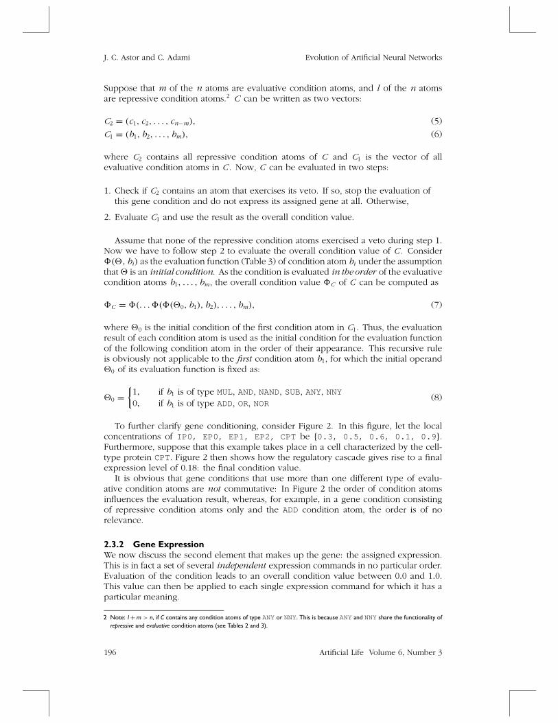
Suppose that m of the n atoms are evaluative condition atoms, and l of the n atomsare repressive condition atoms.2 C can be written as two vectors:

C2 = (c1, c2, . . . , cn−m), (5)

C1 = (b1, b2, . . . , bm), (6)

where C2 contains all repressive condition atoms of C and C1 is the vector of allevaluative condition atoms in C . Now, C can be evaluated in two steps:

1. Check if C2 contains an atom that exercises its veto. If so, stop the evaluation ofthis gene condition and do not express its assigned gene at all. Otherwise,

2. Evaluate C1 and use the result as the overall condition value.

Assume that none of the repressive condition atoms exercised a veto during step 1.Now we have to follow step 2 to evaluate the overall condition value of C . Consider8(2, bi) as the evaluation function (Table 3) of condition atom bi under the assumptionthat2 is an initial condition. As the condition is evaluated in the order of the evaluativecondition atoms b1, . . . , bm, the overall condition value 8C of C can be computed as

8C = 8(. . . 8(8(20, b1), b2), . . . , bm), (7)

where 20 is the initial condition of the first condition atom in C1. Thus, the evaluationresult of each condition atom is used as the initial condition for the evaluation functionof the following condition atom in the order of their appearance. This recursive ruleis obviously not applicable to the first condition atom b1, for which the initial operand20 of its evaluation function is fixed as:

20 ={1, if b1 is of type MUL, AND, NAND, SUB, ANY, NNY

0, if b1 is of type ADD, OR, NOR(8)

To further clarify gene conditioning, consider Figure 2. In this figure, let the localconcentrations of IP0, EP0, EP1, EP2, CPT be {0.3, 0.5, 0.6, 0.1, 0.9 }.Furthermore, suppose that this example takes place in a cell characterized by the cell-type protein CPT. Figure 2 then shows how the regulatory cascade gives rise to a finalexpression level of 0.18: the final condition value.

It is obvious that gene conditions that use more than one different type of evalu-ative condition atoms are not commutative: In Figure 2 the order of condition atomsinfluences the evaluation result, whereas, for example, in a gene condition consistingof repressive condition atoms only and the ADD condition atom, the order is of norelevance.

2.3.2 Gene ExpressionWe now discuss the second element that makes up the gene: the assigned expression.This is in fact a set of several independent expression commands in no particular order.Evaluation of the condition leads to an overall condition value between 0.0 and 1.0.This value can then be applied to each single expression command for which it has aparticular meaning.

2 Note: l+m > n, if C contains any condition atoms of type ANYor NNY. This is because ANYand NNYshare the functionality ofrepressive and evaluative condition atoms (see Tables 2 and 3).



Overall condition value:Φ Φ

SUB

0.2

MUL

0.18

0.18(0.3, 0.1) (0.2, 0.6)

SUB[EP2] MUL[EP1]

ANY

C :

C :

1

=> okay => okay

[EP0]=0.5

C :2

Cell is

of Type CPT

SUP[CPT]ANY[EP0]

SUP[CPT]MUL[EP1]SUB[EP2]ANY[EP0]ADD[IP0]

Θ = 00

Φ

0.3

ANY[EP0]

(0.3, 0.5)Φ

0.3

ADD(0, 0.3)

ADD[IP0]

Figure 2. A gene condition C can be represented as two chains of subconditions: C1 contains the repressive conditionatoms, C2 contains all evaluative condition atoms. First, C1 is checked for condition atoms leading to complete generepression. If there are none—like in this example—C2 is evaluated numerically and determines the overall conditionvalue.

In the following, we discuss every expression command in detail. An overview isgiven in Table 4.

2.3.3 Developmental CommandsTo encode the growth process, special processes are necessary. Developmental com-mands control the construction of new connections between neurons, as well as celldivision.

Table 4. Overview of expression commands. Growing axons/dendrites follow the substrate gradientuntil a local maximum is reached then connect to the cell if one exists at that location. Strengthen-ing/weakening is a percentage increase/decrease of connection weights, determined by the product ofthe last neurotransmitter (here NTx) influx at each connection and the value of the gene condition.The cell-type protein assigned to a cell division command determines the type of the future offspringcell. In this example, the offspring will be of type CTPx and therefore produce cell-type protein CTPxcontinuously. “Relaxing” weights means bringing the specific weights for neurotransmitter NTx influxslightly closer to the initial value 1.0.

Expression Command description Influence ofcondition value

PRD[XY] produce substrate XY production quantityGDR[XY] grow dendrite following gradient of XY probability to growGRA[XY] grow axon following gradient of XY probability to growSPL[CTPx] divide. Offspring is of type CTPx probability to splitEXT excitatory stimulus increase rateINH inhibitory stimulus decrease rateMOD+[NTx] increase connection weights strengthening factorMOD-[NTx] decrease connection weights weakening factorRLX[NTx] relax weights slightly multiplierDFN[NTx] define the type of neurotransmitter noneNOP null action, neutrality



The growth of axons and dendrites must be guided in some way to their target. Invivo this is accomplished either by guidance via surface proteins or with the help ofdiffusible growth factors. To implement the latter, two expression commands exist inthis model:

• GDR(grow dendrite), and

• GRA(grow axon).

In the genome, these commands are always used in conjunction with a diffusible sub-strate, like external proteins or cell-type proteins (e.g., GDR[CTP0]). Once expressed,a connection—either a dendrite or an axon—starts to grow following the local gradientof the substrate (here the protein CTP0). If the growing connection reaches the locationwith the highest local concentration of the particular substrate, it tries to connect to thecell. If no cell is present at this location, or the cell is not of the right type (e.g., itdoes not make sense to connect a dendrite to an actuator), the growing connectiondies. In all other cases, the connection will be established. Plate 2 shows an exampleof dendritic growth.

Another important feature of development is cell division. In this model, a neuroncell can create an offspring cell via the expression command SPL, which is always usedin combination with a cell-type protein. For example, the expression of the commandSPL[CPT0] gives rise to the following behavior: First, one of the surrounding freegrid elements (those locations that do not harbor a neuron cell) is chosen randomly.It is subsequently transformed to a neuron under conservation of its current diffusiblesubstrates. Finally, after separation from the mother cell, the new offspring cell bearsthe same genotype as its mother, except that it can be of a different type (indicated bythe cell-type protein). In vivo, differentiation through cell lineage is very common.

The role condition values play for the expression of developmental commands issubject to the configuration of the simulation environment. The most important caseseems to be its interpretation as a probability for gene expression, leading to condi-tioned development. For instance, a gene like ADD[EP0] -> GDR[CPT0] would leadto dendritic growth as a function of the concentration of the diffusible substrate EP0,just like growth factors do in vivo.

2.3.4 LearningAs is well known, the actual concentrations of neurotransmitter inside of a neurondepend on the weighted influx. A specific weight for each type of neurotransmitter isassigned to each dendritic connection. Initially, the weight of a new connection is setto 1.0, which is considered the relaxed state. However, it can be manipulated by threedifferent expression commands:

• MOD+[NTx] strengthens dendritic connections,

• MOD-[NTx] weakens dendritic connections,

• RLX[NTx] relaxes dendritic connections.

Each command is specific to a neurotransmitter. In this example the commands in-fluence weights used for influx of neurotransmitter NTx. The first two commands—ifexpressed in neuron j—change each synaptic weight in accordance to

∀i: 1wij [NTx] = ±(wij [NTx] ∗ ai ∗ c) , (9)



dendritic connection.concentrations of SPT0, it starts to grow a

gradient of SPT0, ...

f) t=9 ... and establishes the dendritic connection.the sensor cell ...

a) t=4. The sensor cell just started to produce SPT0. b) t=5. Once the neuron cell has detected non-zero

e) t=8. Finally, the growing dendrite approaches

c) t=6. The growing dendrite follows the d) t=7 ... while the sensor cell-type protein keepson diffusing.

Plate 2. A neuron cell starts to grow a dendritic connection following the gradient of the sensor cell-type proteinSPT0. Finally, a new dendrite becomes established. The gene that was responsible for this behavior is of theform . . . , ANY[SPT0] -> GDR[SPTO], . . . . Note that due to the coarse-grained coloring scheme white gridelements do not imply 0.0 concentrations of SPT0 at this location.

where wij [NTx] is the current specific weight of type NTx between neuron i and neu-ron j , ai is the activation of neuron i, and c is the overall condition value of the genethat expresses the MOD+(respectively MOD-) command. As the multipliers ai and c areranged in [0.0;1.0] and furthermore all weights wij [NTx] are set to 1.0 initially, it canbe concluded that

∀i, j : wij [NTx] ≥ 0 . (10)

Non-negative weights may appear to be a limitation, because they do not allow realinhibitive influence. The usage of several types of neurotransmitter, however, makesinhibitive stimulation possible anyway (Figure 3).



w = 0.4

eNT

NTx

eNT

w = 0.1

34

14

expression24

w = 0.3

neuron

neuron

a = 0.82

SUB[NTx]ADD[eNT]

EXT

Genome

neuron

neuron 1

4

2

3

a = 0.7

a = 1.03

1

Genegene

condition

gene

Figure 3. Simple inhibitive connection. The dendritic input from neuron1 and neuron2 produces an eNT concentra-tion of 0.31. Neuron4, however, does not become excited because the NTx concentration represses the gene.

Unlike MOD+and MOD-, the RLX expression command relaxes weights. In lieu ofshaping them, RLX changes individual weight characteristics towards their initial value1.0. Applying RLX to the specific neurotransmitter NTx in neuron j has the followingeffect:

RLX[NTx] H⇒ ∀i 1wij [NTx] =+wij [NTx] ∗ Cp ∗ Cc, if wij [NTx] > 1.0−wij [NTx] ∗ Cp ∗ Cc, if wij [NTx] < 1.00.0, otherwise ,

(11)

where wij [NTx] is the specific weight controlling the flux of neurotransmitter NTx be-tween neuron i and neuron j , Cp is a fixed percentage constant and Cc is the overallcondition value of the gene that expresses the RLX[NTx] command. An internal mech-anism avoids oscillation around 1.0, by ensuring that if a weight is currently greater than1.0 then its future value will be ≥ 1.0 also (and vice versa for weights less than 1.0).

2.3.5 StimulationTwo commands influence cell stimulation in a simple and direct way. Dependingon the value of the gene condition, EXT increases the activation level, while INHcommand decreases it. Both commands do this with respect to the activation range[0.0;1.0] . If during the same time step EXT or INH are expressed more than once,then the effective change of activation is just the sum of all single increases (respec-tively, decreases). Thus, a gene like ADD[IP0] MUL[EP1] -> EXT EXT where thecurrent concentrations of IP0 and EP1 are 0.4 and 0.3 would lead to an activationincrease of 0.24. Unless it is already completely inactive, the cell activation normallydecreases at each time step with an adjustable rate if no stimulation command is ex-pressed.

Obviously, cell stimulation does not necessarily depend on the weighted sum of in-puts. Influences of every kind can manipulate the degree of activation of a cell. Ofcourse, if the modeling of a neuron cell in accordance to classical ANN models isnecessary, this can still be achieved by using neurotransmitter-related condition atomsonly in gene conditions. For example, a gene like ADD[eNT] -> EXT stimulates theneuron according to the weighted sum of inputs (of the default neurotransmitter), justas standard ANN models do. Keep in mind, however, that in vivo, hormones, neuro-



modulators, and other substrates can have a tremendous influence on cell stimulation.This can be easily modeled with, for example, a gene like: ADD[eNT] MUL[EP0] ->EXT. Here, the neuron becomes stimulated according to the weighted sum of inputsand the current concentration of a “neuromodulator” EP0.

2.3.6 Other CommandsCommand PRD, when expressed, produces new substrate (i.e., increases the concentra-tion of a particular substrate). By definition, only the synthesis of external and internalproteins is allowed, as neurotransmitters and cell-type proteins have an implicit role inthe model.

For the expression command PRD, the overall condition value simply determineshow much of the assigned substrate has to be produced. For example, if the currentconcentrations of IP2 and eNT are 0.6 and 0.1, the gene ADD[IP2] AND[eNT] ->PRD[EP2] produces 0.1 of EP2.

Another command is DFN[NT] where NT stands for any neurotransmitter. Onceexpressed, it changes the defined neurotransmitter used for dendritic-axonal injection.The condition value is of no importance for this expression command, as long as it is notequal to 0.0. This command is added because it is known that in vivo, some neuronschange the type of neurotransmitter used at their synapses. Starting with several types,the maturation process of each neuron eventually defines the right type.

Finally, the last expression command to mention is NOP—the neutral command—which takes the role of a placeholder for future genetic changes (i.e., mutations).

2.4 Simulation of the OrganismThe tissue of cells produced by gene expression and cell growth is termed an artificialorganism. It receives input from the environment (the outside world) and can act onit by signaling to the environment via its actuators. In the simplest case, the organismreceives and generates patterns of activation.

A simulation always starts by creating sensor and actuator cells. Their number isdetermined only by the complexity of the outside world and is not coded for in thegenome. In other words, these cells really represent possible signals and actuations inthe world, not actual signals and actuations performed by the organism. An organismchooses to receive input or perform an actuation by connecting to these cells. Ifneeded, an additional reinforcement cell can be created. This is a special sensor cell(with its own cell-type protein) used to provide a reinforcement signal from the worldabout the behavior of the organism. Whether or not this signal is used depends on thegenome.

At the start of simulation for each new artificial organism, one initial neuron is placedin the center of the grid. After initialization, the simulation begins. Input from theworld is provided to the sensor cells, cell-type proteins and external proteins diffuse,and neurons execute their genetic code. This is done synchronously to guaranteeconsistency in the artificial chemistry.

Depending on its gene expression, a neuron starts growing axons and dendrites,produces offspring cells, and might initiate cell differentiation. Gene expressions maylead to protein production cascades, stimulation, and ultimately information exchangebetween neurons. After every simulation cycle the network’s “fitness” is determinedby comparing any inputs and outputs to what is expected in this particular world, pro-ducing a real-valued reinforcement signal between 0.0 (punishment) and 1.0 (reward).This signal can be used by the organism if a reinforcement sensor is present and if theorganism chooses to connect to it.



3 Examples: Genes and Networks

The best way to validate and evaluate this model would be to let the system evolveANNs for specific environments. This, however, is not done yet for reasons discussedlater on. Except for some experiments in which simple logical functions were evolvedfrom scratch [3], most genomes were handwritten. To show that the model is able togive rise to networks that perform some key behaviors known from biology, examplesof handwritten genotypes and the resulting phenotypes are given in the following,performing self-limiting growth, networks that perform logical functions, and classicalconditioning. Other examples of physiologically important structures that have beenreproduced are the regeneration of injured networks, pacemaker behavior, as well assensitization and habituation behavior [3].

3.1 Self-limiting GrowthThe development of natural systems is based on a decentralized growth process thatarises from local gene expression in each single cell. This, combined with the factthat inhibition is necessary to avoid unbounded growth, means that self-inhibition is anessential property the model has to encompass. For example, self-limitation is essentialto avoid cancerous growth. The following genome shows how self-limited growth canbe achieved in a simple way in a completely local manner. In the genome below, Crefers to the regulatory (conditional) part of the gene, and E is the code to be expressed:

Gene 1 C: SUP[cpt] NNY[ip0]E: PRD[ep0] PRD[ip0]

Gene 2 C: ADD[ep0]E: SPL[acpt0]

Gene 3 C: NNY[ip0]E: GRA[acpt0] PRD[ip0]

Gene 4 C: ANY[ip0]E: PRD[ip0]

The first gene is expressed initially by the stem cell that produces cell-type proteincpt . As no internal protein ip0 is present initially, gene 1 is expressed and leads tothe production of the external protein ep0 and the internal protein ip0 . Just like everyexternal protein, ep0 diffuses within the tissue so that the initial peak concentrationin the stem cell becomes weaker while surrounding cells receive concentrations ofep0 . Gene 4 guarantees that once a cell harbors any ip0 it is going to produce ip0constantly from then on. This, however, suppresses gene 1, which consequently willnever produce ep0 again. The internal protein ip0 also suppresses gene 3, whoseexpression leads to axon growth and ip0 production. Thus, a cell in which initially noip0 is present starts growing an axon and then suppresses itself continuously via gene 4.

Gene 2 can lead to cell division. Every executed split command creates a newoffspring cell of type acpt0 . However, cell division occurs only with a probability thatis proportional to the current concentration of ep0 . Thus, as ep0 diffuses away overtime, cell division becomes less and less probable. Consequently the growth processremains limited. This effect can be observed in Plate 3, which shows snapshots takenfrom a simulation of the genome above.

3.2 Logical FunctionsResearch in neurobiology has shown [15] that some neural structures essentially im-plement fixed logical functions. Using two different kinds of neurotransmitter, logicalgates can be simulated easily within the present model (Figure 4).



t=2

t=300

t=5

t=10 t=50

t=150

Plate 3. Self-limiting growth. An initially high peak of a diffusible substrate facilitates cell division. As the substratevanishes over time, fewer cell divisions occur.

The basic logic operations AND, OR, NOT are sufficient for the construction ofany logical function. For example, the genome shown below constructs the functionD = (A → B) ∨ C , where A, B, C are sensor signals and D is the resulting actuatorsignal. To model this logical function, one has to combine an implication gate (i.e.,¬A ∨ B) with an OR gate.

Using both the genetic fragments of Figure 5, a genotype can be constructed thatgrows the appropriate ANN structure and describes the stimulation behavior:

Gene 1 C: SUP[cpt] NNY[ip0] ANY[spt0] ANY[apt0]E: SPL[acpt0] GRA[apt0] GDR[spt0] PRD[ip0]



ANY[NT1] -> EXT

Genes:

NT0

NT1

OR

ANY[NT0] -> EXT

Gene:

Simple binary-logic gates:

Simple fuzzy-logic gates:

NT0

NT1

NT0

NT1

ORNT0

NT1

AND

ANY[NT0] ANY[NT1] -> EXT

ADD[NT0] OR[NT1] -> EXT

AND

ADD[NT0] AND[NT1] -> EXT

NOTNT0

NAND[NT0] -> EXT

Gene:

NOTNT0

NNY[NT0] -> EXT

Gene:

Gene: Gene:

Figure 4. Logical gates and the genomes that perform them. Any logical gate can be simulated easily in the modelas long as the incoming signals use two different types of neurotransmitter.

NT1

from A:

from B:

A->B D

from C:

NT1

Genes:

ANY[NT1] -> EXT

Genes:

eNT

eNT

ANY[eNT] ANY[NT1] -> EXT

NNY[eNT] -> EXT

ANY[eNT] -> EXT

Figure 5. The stimulation model for an ANN structure performing D = (A→ B) ∨ C.

Gene 2 C: SUP[acpt0] NNY[ip0] ANY[spt2] ANY[cpt]E: GRA[cpt] SPL[acpt1] GDR[spt2] DFN[NT1] PRD[ip0]

Gene 3 C: SUP[acpt1] ANY[spt1] NNY[ip0] ANY[acpt0]E: DFN[NT1] GRA[acpt0] PRD[ip0] GDR[spt1]

Gene 4 C: ANY[ip0]E: PRD[ip0]

Gene 5 C: SUP[cpt] ANY[NT1]E: EXT

Gene 6 C: ANY[eNT] NSUP[acpt0]



A

spt2

spt1

D

spt0

acpt1

NT1

NT1

Sensors: A->B

acpt0 cpt

(A->B) v C Actuator

apt0

C

B

A

Figure 6. Schematic representation of the ANN realization of D = (A→ B) ∨ C. The type of neurotransmitter ismarked next to the axon if a nondefault neurotransmitter is used. Cells are named by the cell-type protein theyproduce. The cell of type acpt1 is used as “neurotransmitter-switch.”

E: EXTGene 7 C: SUP[acpt0] ANY[eNT] ANY[NT1]

E: EXTGene 8 C: SUP[acpt0] NNY[eNT]

E: EXT

Genes 1–3 lead to the morphological structure of the network. The neuron of cell-type protein cpt produces an offspring cell of type acpt0 that models A→ B, whilethe cpt cell represents the OR gate. Three different cell types are needed because thelogical function requires different kinds of neurotransmitter whereas the sensors useonly eNT. Thus, an intermediate cell is necessary to overcome this problem. Gene 4is the usual suppression gene that becomes active once one of the first three genes isexpressed. Genes 5 through 8 encode the stimulation behavior in accordance to thedifferent types of cells.

The genome for this task might, at first sight, appear rather long. However, oneshould keep in mind that it describes the construction of a fully deterministic struc-ture, which is more difficult for a growth model than for an approach based on di-rect encoding. Furthermore, simpler genomes can be built that model the same log-ical function. This example is intended to show that every logical function can beconstructed by connecting simple gates leading to hierarchical structures not unlikethose found in real networks. A schematic representation of the resulting structure isshown in Figure 6. As the paths of the input signals from the sensors to the com-putation units are of different lengths, a particular input has to be present at thesensors for several subsequent time steps before a stable output signal will be pro-duced.

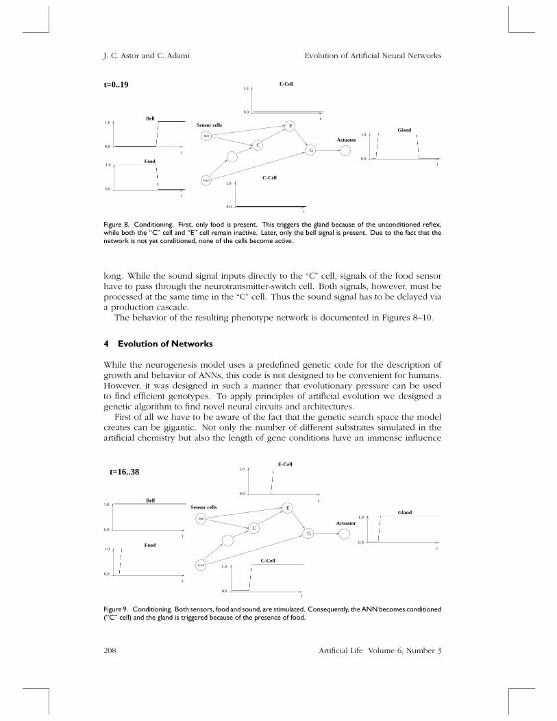
3.3 Classical ConditioningPlate 4 documents the development of a simple ANN that displays conditioned re-flex behavior as in Pavlov’s classical experiment [18]. Suppose the sensor on thelower left side in Plate 4 is stimulated at the sound of a bell. Further, suppose theupper left sensor is an optical stimulus representing the presence (or absence) offood. Finally, let us imagine that the actuator on the right side triggers a salivarygland if food is present. This behavior is the unconditioned reflex. The above net-work can learn to associate this reflex with a condition: the sound of the bell. If



t=0 cycles

t=10 cycles

t=6 cycles

t=8 cycles

Plate 4. Development of the network for classical conditioning.

presence of food and the ringing of the bell are associated repeatedly, the networkwill learn to trigger the gland even if only the bell rings. If after the conditioningthe bell rings without presence of food, the association will gradually, but steadily,weaken.

Such a behavior can be modeled using different kinds of cell types. One cell (“C” cell)is activated if the network is in the conditioned state, which means that the acousti-cal and optical stimulus have been present together before. Another cell (“E” cell) isactivated if the acoustical stimulus is currently present and the network is in the con-ditioned state at the same time. If so, a cell (“G” cell) representing the trigger of thesalivary gland is activated. Of course, the “G” cell also has to be activated if only foodis present. This is the unconditioned reflex. A schematic drawing of the network isshown in Figure 7.

The genome that encodes the development and behavior of this network is shownbelow.

Gene 1 C: NNY[ip0] SUP[cpt] ANY[spt0]E: SPL[acpt0] PRD[ip0] SPL[acpt2] GDR[spt0] DFN[NT1]

Gene 2 C: NNY[ip0] SUP[acpt0] ANY[spt1] ANY[cpt]E: PRD[ip0] GDR[spt1] GRA[cpt] DFN[NT1]

Gene 3 C: ANY[spt1] SUP[acpt2] NNY[ip0] ANY[apt0]E: SPL[acpt1] GDR[spt1] PRD[ip0] GRA[apt0]

Gene 4 C: ANY[acpt2] SUP[acpt1] ANY[spt0] NNY[ip0]E: GRA[acpt2] GDR[spt0] GDR[cpt] PRD[ip0]

Gene 5 C: ANY[ip0]



E

G

C

Bell

eNTNT-switch

eNT

eNT

eNT

eNT eNT

NT1

Sensor cells Actuator

Food

acpt1

acpt2

acpt0

spt0

spt1

apt0

cptNT1

Figure 7. A schematic representation of the network for classical conditioning. The types of neurotransmitter usedare marked next to the axons. The cell-type protein used by each cell is indicated near the cell body.

E: PRD[ip0]Gene 6 C: NSUP[cpt] NSUP[acpt1] ADD[eNT]

E: EXTGene 7 C: SUP[acpt1] ADD[NT1] MUL[eNT]

E: EXTGene 8 C: ADD[eNT]

E: PRD[ip1]Gene 9 C: ADD[ip1]

E: PRD[ip2]Gene 10 C: SUP[cpt] ADD[NT1] MUL[ip2]

E: PRD[ep0]Gene 11 C: SUP[cpt] ADD[ep0]

E: EXT

Genes 1 to 4 control cell division into the different types that are needed, as wellas the growth of axons and dendrites. Gene 5 is the usual stop gene. To be able todistinguish between two different kinds of signals, two types of neurotransmitter haveto be used. The “C” cell, for example, uses NT1 as neurotransmitter so that the “E” cellcan check for inputs from the acoustical sensor and from the “C” cell at the same time.The manifestation of this can be seen in the genotype: The cells of type acpt0 andcpt use NT1 instead of the default neurotransmitter eNT (note the expression commandDNF[NT1] ).

The “C” cell also has to make the distinction between two signals: the acoustical andthe food sensor input. As sensor cells use by definition only the default neurotransmit-ter, a kind of neurotransmitter-switch cell is needed between the food sensor and the“C” cell. This is why an additional cell of type acpt0 is needed (gene 2).

While gene 6 takes care of the unconditioned reflex stimulation, genes 7–11 con-trol the conditioning. If food is present and the bell rings, gene 10 produces certainamounts of external protein ep0 (through a time-delay cascade via genes 8 and 9).The concentration of ep0 influences cell stimulation (gene 11). Due to diffusion, ep0diminishes over time, so the conditioning decreases accordingly.

The time delay of eNT inputs via genes 8 and 9 and finally 10 is necessary becausethe dendritic paths from both sensors (food and sound) to the “C” cell are not equally



t=0..19

t

1.0

0.0

t

1.0

0.0

t

1.0

0.0

t

1.0

0.0

t

0.0

1.0

Food

Bell

Sensor cells

ActuatorC

E

G

Bell

Food

E-Cell

C-Cell

Gland

Figure 8. Conditioning. First, only food is present. This triggers the gland because of the unconditioned reflex,while both the “C” cell and “E” cell remain inactive. Later, only the bell signal is present. Due to the fact that thenetwork is not yet conditioned, none of the cells become active.

long. While the sound signal inputs directly to the “C” cell, signals of the food sensorhave to pass through the neurotransmitter-switch cell. Both signals, however, must beprocessed at the same time in the “C” cell. Thus the sound signal has to be delayed viaa production cascade.

The behavior of the resulting phenotype network is documented in Figures 8–10.

4 Evolution of Networks

While the neurogenesis model uses a predefined genetic code for the description ofgrowth and behavior of ANNs, this code is not designed to be convenient for humans.However, it was designed in such a manner that evolutionary pressure can be usedto find efficient genotypes. To apply principles of artificial evolution we designed agenetic algorithm to find novel neural circuits and architectures.

First of all we have to be aware of the fact that the genetic search space the modelcreates can be gigantic. Not only the number of different substrates simulated in theartificial chemistry but also the length of gene conditions have an immense influence

t=16..38

t

1.0

0.0

t

0.0

1.0

t

1.0

0.0

t

1.0

0.0

t

1.0

0.0

Food

Bell

C

E

G

Sensor cells

Actuator

E-Cell

Gland

C-Cell

Food

Bell

Figure 9. Conditioning. Both sensors, food and sound, are stimulated. Consequently, the ANN becomes conditioned(“C” cell) and the gland is triggered because of the presence of food.



t=50..64

t

1.0

0.0

t

1.0

0.0

t

0.0

1.0

t

1.0

0.0

t

1.0

0.0

Food

Bell

C

E

G

Sensor cells

Actuator

Food

Bell

E-Cell

C-Cell

Gland

Figure 10. Conditioning. Being in the conditioned state, the food sensor suddenly becomes inactive while the bellkeeps on ringing. Thus, the activation of the “C” cell becomes weaker. This implies a decrease of activation of the“E” cell that eventually results in a decline of gland activity.

on the number of possible different genotypes. The size of the genetic space is animportant issue for the design of a GA. The bigger it is, the more computation has to bespent on evolutionary search in order to find genotypes that code for interesting ANNs.To compound matters, unlike in usual ANN models, a computational overhead arisesdue to the simulated biological world. In a neurogenesis model such as this, the mapfrom genotype to phenotype is highly implicit as the networks are grown from singlestem cells in a developmental process that involves an enormous computational effort:Substrates are created through gene expression; they undergo diffusion within thetissue; gene conditions have to be evaluated; and so on. Thus, extensive computationis necessary until the fitness of a particular genotype can be determined, and even moreto apply evolutionary search. An increase in computational power can be achieved bya distributed GA that allows a massively parallel search. Details of the implementationof the GA are relegated to Section 5.

4.1 Fitness EvaluationThe fitness of a particular genotype can only be assessed through the fitness of thephenotype it gives rise to in a particular environment. The phenotype’s fitness itselfis defined as the average reinforcement signal received from its environment (see Sec-tion 2.4).

Three levels of assessment determine if an organism passes or fails the evaluationrequest:

1. Knockout criteria: It seems to be reasonable to assign an organism a zero fitness ifit does not fulfill some minimal criteria. For example, organisms in which theactuator and sensor cells are not connected (no dendrite/axon grew to them) areassigned zero fitness by default. Furthermore, organisms in which the actuators areconstantly activated or inactivated are not considered fit either, as no computationcan be achieved. Such organisms are replaced immediately.

2. Organisms that passed the first level are compared with each other on the secondlevel: All organisms occupy a particular position on a ranked list of decreasingfitness. If the relative fitness of the organism that sent the evaluation request isbelow a fixed percentage threshold rank (i.e., it is better than most), then it passesautomatically (Figure 11).



Genotype)rel.

Φ( Genotype)

θj-1 nj-1

νj+1n

j+1

Φ(ζ)with phenotype fitness

Genotype ζ

sends evaluation request

Φ(

of assessment

Position Genotype

0

1

n

ψ

π

ζ

ϖ

j

n0

n

n

1

n

ordered

by decreasing

percentage threshold

}pass

jn

2nd level

Figure 11. Organisms belonging to the elite (defined by a percentage threshold) always survive their evaluationrequest. In this case, organism ζ does not pass the comparison test (i.e., the second level of assessment).

3. As the threshold-based assessment is rather rough, organisms that do not pass thisstep get a second chance: They survive by chance with a probability

P(X < e−c∗prel) (12)

where X is taken from a uniform probability distribution over range [0.0;1.0] , cis a constant, and prel is the relative position (based on fitness) in the ranked list ofall genotypes.

Obviously, the size of the population does not matter in applying these criteria and cantherefore vary over time.

4.2 Genetic OperatorsSelection, recombination and mutation are the genetic operations that are used to buildnew genotypes from a genetic pool. As new genotypes can be constructed in manydifferent ways (by combining the aforementioned operations together with replica-tion), the genetic operations will be presented first before the description of the actualconstruction mechanism follows (Section 4.3).

4.2.1 SelectionOccasionally, the GA-server has to select genotypes from its database. According to theprinciples of artificial evolution, selection has to be based on the fitness of genotypes.As genotype fitness cannot be measured objectively, usually a selection mechanismis applied that chooses genotypes with a probability proportional to their phenotypefitness. Accordingly, the GA server uses a roulette wheel selection.

4.2.2 RecombinationTo recombine two genotypes they have to be aligned. Subsequently, one or morecrossing points have to be chosen at which the hereditary information is exchanged.However, crossover points can only be chosen within genes, so that each gene isprotected and cannot be torn apart across two genotypes. In other words, differentgenes do not swap code fragments. This principle is also found in nature: Only whole



genes undergo recombinational exchange and never parts of genes. The number ofcrossovers is chosen from a binomial probability distribution with an expectation valueclose to one.

Due to mutation (see below) genotypes can differ in length. Naturally, in the caseof crossover of genotypes of different length, the crossover points are chosen inside ofthe overlapping area of the two genotypes.

4.2.3 MutationMutation is necessary to produce diversity in the genetic population. It is applied by theGA-server as a genetic operation and changes a randomly chosen genotype “slightly”(as explained below). In this model, mutation can take place in two ways:

• Point mutations: These are restricted to one gene. A randomly chosen conditionatom or expression command of a randomly chosen gene changes to its nearestneighbor in genetic space. This means that if, for example, the condition atomADD[IP2] has been chosen, mutation changes either the substrate (e.g., toADD[IP1] ) or the operation (e.g., to MUL[IP2] ) but never both.

• Genome mutation: Another important kind of mutation that is found in nature aswell is mutation on the genome level: deletion, insertion, and doubling of entiregenes. For example, successful genes (e.g., structure genes that build a layer ofneurons) can be doubled while other useless genes may vanish entirely. Genedoubling has become a success story in evolution. Indeed, it was shown recently[20] that initially simple morphological genes (sometimes even entire genomes)often doubled during evolution, only to subsequently specialize.

4.3 Construction of GenotypesWhen a genotype has to be replaced because of low fitness or if the size of the popu-lation grows, a new genotype must be constructed. This can be done in several ways:from a random genome, by recombination, by pure “asexual” reproduction (i.e., repli-cation), with or without point mutation, gene insertion, doubling, or deletion. Thereis no way to determine a priori which of them plays the most important role. Forexample, we do not know if recombination of two fit genotypes is in principle betterthan constructing new genotypes with asexual copies of fit organisms. In nature, bothprinciples are applied. Therefore, the different possibilities should all be integratedusing tunable probabilities. Figure 12 describes the algorithm used to construct newgenotypes in this GA as a probability tree.

5 Implementation

A distributed GA can be implemented in two ways: either by using a massively parallelmachine, or by distributing the system over a network of computers. For our purpose,the latter seems to be the better choice, especially if the GA is not limited to a local areanetwork (LAN) and allows platform-independent use. The importance of heterogeneouscomputer networks has been increasing enormously during the last decade and willmost probably be the architecture of the future. Designing the distributed GA as anopen system on a wide area network (WAN, e.g., the Internet) enables us to tap theunused CPU power of a very large number of computers, bringing an extraordinarilycomputationally expensive task into the realm of possibility.

The basic design can be described as follows: Using Sun’s Java technology, anasynchronous, distributed GA system was built that allows a massively parallel searchfor genomes based on evolutionary principles. It consists mainly of a central server



genotype

has to be constructed

construct a new

one by

"sexual" recombination

construct a new

one by

"asexual" reproduction

choose one

from the population

as second parent p2

g=recombination(p1, p2)

new genotype: new genotype:

g=copy(p)

gene insertion

occurs on g

gene deletion

occurs on g

gene insertion

occurs on g

gene deletion

occurs on g

a new

random genome

new genotype g built

point mutation

occurs on g

gene doubling

occurs on g

1-P(recombNewProb)

1-P(newGenomeProb)P(newGenomeProb)

P(recombNewProb)

P(recombProb) 1-P(recombProb)

1-P(pointMutProb_recomb)

P(pointMutProb_recomb)

1-P(delMutProb_recomb)

point mutation

occurs on g

gene doubling

occurs on g

P(dblGenProb_recomb)

1-P(dblGenProb_recomb)

P(addGenProb_recomb)

1-P(addGenProb_recomb)

P(delGenProb_recomb)

1-P(pointMutProb_NotRecomb)

1-P(pointMutProb_NotRecomb)

1-P(dblGenProb_NotRecomb)

1-P(dblGenProb_NotRecomb)

1-P(addGenProb_NotRecomb)

1-P(addGenProb_NotRecomb)

1-P(delGenProb_NotRecomb)

choose one

from the population

choose one

from the population

as first parent p1: as first parent p1: as parent p:as parent p:

build a

random genome

build a

Figure 12. Starting from the top, the diagram describes the different ways to construct a new genotype. Whileunlabeled arrows carry the probability one, constants are assigned to others describing the probability of the arrow tobe chosen. The genetic operations selection (“choose from population”), recombination, and mutation are definedas described in the previous sections.

application and many clients, each of which hosts one individual of the current GApopulation. While the central server drives the evolution via genetic operations (i.e.,recombination, selection, and mutation), the clients represent the population, which ischanging continuously in size and location. By starting a client locally, it can latch ontothe server, and by being a host for one genotype it becomes part of the evolutionaryprocess. It can, of course, detach itself from the evolutionary process at any time. Inthis case, data about the hosted genotype (and the phenotype it has grown) are sent



Central GA-server,

131.215.48.50

somewhere

Organism as Appletin a browser, onarchitecture ’foo’, Organism as Applet

157.215.120.2in a browser, e.g., on

e.g., on Sun SPARC

Ensemble of currently

active organisms

an i86-PCOrganism, e.g., on

Sun SPARC 141.7.12.105Organism, e.g., on

Ensemble of currently

suspended organisms

Plate 5. Genotype evaluation in clients of different architecture, using TCP for communication with the asyn-chronous GA.

back to the server where they will be stored until another client receives the data onits registration request.

In the following, we will use both the terms organism and phenotype synonymouslyfor the cell structure that has been grown from one stem cell of a particular genotype.We use the term new organism for a newly created stem cell that has yet to perform anygene expression. Note that each organism is distinguished by its particular genotypeand contains it as its genome inside. Thus, an organism always contains the hereditaryinformation from which it was grown. Consequently, the server only has to maintain adatabase of organisms.

As Java is supposed to be platform independent, clients can be started from everycomputer for which an accurate Java virtual machine or browser exists and can thencommunicate via the Transport Control Protocol (TCP) with the central server (Plate 5).

To make the system as flexible as possible the clients can be designed as hybrids,which means that they can be started either as a Java Applet by choosing a specificHTML (Hypertext Markup Language) page from a particular WWW server, or as a Javaapplication with the help of a bootloader program that dynamically downloads theclient and starts it as a Java application; in the latter case, no browser is necessary.

This dynamical and platform-independent design balances Java’s disadvantage inbeing a slow, interpreted language. Increasing computer performance and faster exe-cution of Java byte code via just-in-time (JIT) compilation will make Java even bettersuited for this purpose in the future.

5.1 Communication Between Clients and GA ServerA client automatically sends a request-to-register to the central GA server after it isstarted and receives from the server a (new) organism ζ . The client then starts up a



often

S

S suspended

Database of

organisms

A A✕ all

Database of

organismsarbitrarily

2.) ... otherwise, construct a new organism

new client central GA-server

register request

evaluation request

STOP

o.k.

{ Comparison

1.) Take a suspended one if any, or ...

(new) organism reply

new organism or ’go on’ reply

check-out request (organism)

Figure 13. Communication between GA server and client hosting an organism.

simulation as described in Section 2.4. After a certain number of simulation cycles, itsends the organism’s fitness 8(ζ) to the server. By comparing 8(ζ) to the fitness ofother phenotypes in the database (as described in Section 4.1), the server decides ifit is worthwhile to keep this organism or if the client should be assigned a differentone. If the server has to send a different organism, it either takes a suspended one outof its database, or constructs one through the processes of recombination or asexualcopying from genotypes of known fitness already present in the population (Figure 13).Fitter genotypes are more likely to be selected for recombination or asexual copyingthan genotypes of lower fitness. This leads to an increase of the average fitness ofphenotypes over time.

A particular client repeats its evaluation request arbitrarily often and always eitherobtains the permission to go on with the same organism or receives a different organismto evaluate. If the client (or better: the human who started the local client) decides toend its participation, it just sends the phenotype back to the GA server, which stores itin its database of currently suspended organisms.

5.2 Participating in Evolution ExperimentsTo facilitate the participation in evolutionary experiments across the Internet, sitehttp://norgev.alife.org has been created, from which the Java application canbe downloaded. This site also offers instructions and more detailed system require-ments.

5.3 Performance and System LimitationsUp to now, only very simple ANNs for logical basic functions have been evolved denovo [3]. The system was able to accomplish this in a short amount of time with apopulation of about 40 genotypes running on about 10 Sun SPARC Stations 2. Whilethis experiment showed that the genetic algorithm works for small populations, it hasnever had to deal with populations of a large size.

If the system is to be opened to the whole Internet community, a more appropriatedatabase organization may be necessary. While the implementation with Java hash



tables might be good enough for small populations, it is surely restrictive for largepopulations. Instead, the system ought to be connected to a professional databasesystem in order to be able to deal with high rates of server requests and large amountsof data.

The current implementation uses Java on both sides: Clients (Java Applets) and serverare fully based on Java technology aided by the remote method invocation technique.However, in principle there is no need for the server to be implemented in JAVA. Abetter approach would be to implement the GA server as a plain CORBA server in anative language such as C++. This would provide a significant performance boost onthe server side and, furthermore, would allow easier access for other applications dueto the open CORBA standard.

The system has been implemented with the help of Java Development Kit (JDK)1.1.5. It has been tested on three different kinds of operating systems: MS-Windows95, Solaris 2.5.1, and FreeBSD 2.2.2. Using the Java virtual machines included in theJDK 1.1.5 (FreeBSD and Win95) and JDK 1.1.3 (Solaris) the system appears to workfine. However, no tests have been done on any versions newer than JDK 1.1.5. Totake advantage of the new system improvements of Java 2 (such as the aforementionedCORBA architecture), the entire system would have to be migrated.

Although computer performance increases continuously, Java—as an interpretedlanguage—is still slow and its computational power therefore very limited comparedto compiled program code. As a consequence, we chose to fix the size of the artificialtissue to 12 × 12, even if any arbitrary size can be chosen. Even if the emergenceof the JIT compilation techniques by themselves improved the system’s performance,more computational power on the client side seems to be necessary to overcome thelimitations mentioned. Increasing the size of the tissue would have several advantagesand allow the growth and evolution of larger networks. Also, artifacts caused by theboundary elements and the rough granulation (which affects the smooth diffusion ofsubstrates) might be avoided in such larger tissues.

6 Conclusions

There are many steps that remain to be taken in the future. First of all, the systemhas to be evaluated in more depth. Experiments should be performed that attempt toevolve simple ANNs for a given world, rather than the simple examples presented herethat were largely world independent. Finally, evolution experiments should be startedin earnest to validate the central premise of this work, namely that complex networkswith novel characteristics can emerge within the present setting.

Apart from this, there is no doubt that the genetic language (the artificial chemistry),invented rather spontaneously and without much rigorous and quantitative testing, canbe optimized. For example, it would be interesting to see if the set of condition atomscan be reduced to a minimum. Simple considerations about the size of genetic spaceand the fitness landscape it gives rise to [3] show that reducing the number of differentcondition atoms would make the computational overhead much less daunting.

Further, certain enhancements might be suitable for future versions of the model.Fleischer [8] showed the importance of a dynamic morphology for the development ofnatural-like systems. At present, our model does not feature morphology. Cells arelocated at the same place from their birth on. Cell death does not exist. Additionalexpression commands that allow, for example, cells to move along a chemical gradientwould be a good way to incorporate morphology into the model. Cell death could beanother interesting issue that would bring the model closer to real neural development.

One of the driving principles of this model is that of locality. First and fore-most, the behavior of each neuron is determined by local concentrations. A more



sophisticated model would take other local structures (besides neurons) into accountas well. Dendrites and axons exist in the current model only as shortcuts betweenneurons. They do not, at present, have any local structural features. For future ver-sions maybe a separate part of the genome could describe the behavior and structureof dendrites and axons. If so, synaptic changes could be coded and based on lo-cal conditions rather than cell-global conditions. For instance, external proteins couldthen directly affect synapses at the site of the synapse just like neuromodulators do invivo.

During natural cell division, cellular substrates are not divided equally between pre-cursor and progeny cell. Differences in both cells can lead to different gene expressionsthat are important for development based on cell lineage. Currently, this is not the waycell division takes place in the model. Even more unrealistically, the progeny cell sim-ply inherits all substrates of the grid element that it replaces. This could be refined infuture versions.

To bring the model closer to biology, a possible consideration is to consider includingcell membranes in the model. At the moment, a cell membrane exists only in the sensethat internal proteins and neurotransmitters cannot diffuse out of the cell. All other typesof substrate can go into and out of the cell plasma. Natural cell membranes are knownto be functional (they trigger cell-internal events) and highly selective, and thereforethey influence the cell’s information processing to a high degree. It is, however, difficultto tell if including this would improve the model or if computational performance wouldonly suffer even more from the increase of complexity.

This work introduced a developmental and behavioral model based on artificial geneexpression that shares key properties with natural neural development. The heart of themodel is the coding scheme of genotypes. The genetic code allows for the descriptionof information-processing structures that show behavior similar to certain natural sys-tems, within a coding scheme that borrows heavily from the gene-regulation paradigm.Without undue effort, genotypes for ANNs can be constructed that are believed to be es-sential [12, 15] for higher self-organizing information-processing systems, such as deter-ministic structure development, self-limiting cell growth, regenerative structures, growthfollowing gradients of diffusive substrates, computation of logical functions, pacemakerbehavior, and simple adaptation (sensitization, habituation, associative classical condi-tioning). Assuming that these phenomena are essential for natural intelligence, it maybe surmised that the model allows—in principle—the description of more complexinformation-processing structures.

Our primary thrust in reducing the gap between the physiology of neurons andthe abstract models that are supposed to model them was to reduce the mathemati-cal abstraction of neurons by reverting to more low-level structures, in the hope thatabstract neurons would emerge. This is the classical artificial life approach that hasserved well in many other applications. Unfortunately (but predictably) the freedomgained is associated with large genotypes (noncompact descriptions) and an expo-nentially large genetic search space. We described how an evolutionary search forgenomes coding for information-processing network structures can be distributed ina platform-independent manner such that the unused CPU power of the Internet canbe tapped to search for ANNs that reduce the gap between the abstract models andneurophysiology.

Experiments on a large scale remain to be done and the model needs to becomemore sophisticated. However, this approach shows that physiology and architecturecan be encoded in one genotype, such that it gives rise to the development of ANNsbased on local interactions only. Further, the platform-independent and fully WWW-distributed system is a new and sophisticated strategy to approach problems based onevolutionary search.



AcknowledgmentsThis work was supported in part by the NSF under grant PHY-9723972, as well as afellowship of the Studienstiftung des Deutschen Volkes to J.A.

References1. Ackley, D. H., & Littman, M. L. (1992). Interactions between learning and evolution. In

C. G. Langton, C. Taylor, J. D. Farmer, & S. Rasmussen (Eds.), Artificial life II(pp. 487–509). Redwood City, CA: Addison-Wesley.

2. Adami, C. (1998). Introduction to artificial life. Santa Clara, CA: TELOS Springer.

3. Astor, J. C. (1998). A developmental model for the evolution of artificial neural networks:Design, implementation, and evaluation. Diploma thesis, University of Heidelberg,Germany.

4. Bower, J. M. (1995). The book of GENESIS: Exploring realistic neural models with theGEneral NEural SImulation System. Santa Clara, CA: TELOS Springer.

5. Britten, R. J., & Davidson, E. H. (1969). Gene regulation for higher cells: A theory. Science,165, 349–357.

6. Britten, R. J., & Davidson, E. H. (1971). Repetitive and non-repetitive DNA sequences and aspeculation on the origins of evolutionary novelty. Quarterly Review of Biology, 46,111–138.

7. Fahlman, S. E., & Lebiere, C. (1990). The cascade-correlation learning architecture. InD. S. Touretzky (Ed.), Advances in neural information processing systems 2 (pp. 524–532).San Mateo, CA: Morgan Kaufmann.

8. Fleischer, K. (1995). A Multiple-mechanism developmental model for definingself-organizing geometric structures. Unpublished doctoral dissertation, California Instituteof Technology.

9. Fritzke, B. (1992). Growing cell structures—A self-organizing network in k dimensions. InI. Aleksander & J. Taylor (Eds.), Artificial neural networks II (pp. 1051–1056). Amsterdam:North-Holland.

10. Gruau, F. (1992). Genetic synthesis of Boolean neural networks with a cell rewritingdevelopmental process. In D. Whitley & J. D. Schaffer (Eds.), Combination of geneticalgorithms and neural networks. IEEE Computer Society Press.

11. Hopfield, J. J. (1982). Neural networks and physical systems with emergent collectivecomputational abilities. Proceedings of the National Academy of Sciences, 79, 2554–2558.

12. Kandel, E. R., & Schwartz, J. J. (1991). Principles of neural science. Amsterdam: Elsevier.

13. Kitano, H. (1990). Designing neural network using genetic algorithm with graph generationsystem. Complex Systems, 4, 461–476.

14. Kitano, H. (1998). Building complex systems using developmental process: An engineeringapproach. Lecture Notes on Computer Science, 1478, 218–229.

15. Koch, C., & Poggio, T. (1982). Biophysics of computation: Neurons, synapses andmembranes. In G. M. Edelman, W. E. Gall, & W. M. Cowan (Eds.), Synaptic function(pp. 637–697). New York: Wiley.

16. Langton, C. G. (Ed.). (1995). Artificial life: An overview. Cambridge, MA: MIT Press.

17. Michel, O. (1996). An artificial life approach for the synthesis of autonomous agents. InJ. M. Alliot, E. Lutton, & E. Ronald (Eds.), Artificial evolution, Lecture Notes in ComputerScience 1063 (pp: 220–231). Berlin: Springer.

18. Pavlov, I. P. (1927). Conditioned reflexes: An investigation of the physiological activity of thecerebral cortex. London: Oxford University Press.

19. Pitts, W., & McCulloch, W. S. (1943). A logical calculus of the ideas immanent in nervousactivity. Bulletin of Mathematical Biophysics, 5, 115–133.



20. Postlethwait, J. H., Yan, Y. L., Gates, M. A., Horne, S., Amores, A., Brownlie, A., Donovan,A., Egan, E. S., Force, A., Gong, Z. Y., Goutel, C., Fritz, A., Kelsh, R., Knapik, E., Liao, E.,Paw, B., Ransom, D., Singer, A., Thomson, M., Abduljabbar, T. S., Yelick, P., Beier, D., Joly,J. S., Larhammar, D., Rosa, F., Westerfield, M., Zon, L. I., Johnson, S. L., & Talbot, W. S.(1998). Vertebrate genome evolution and the zebrafish gene map. Nature Genetics, 18,345–349.

21. Vaario, J. (1994). Modeling adaptive self-organization. In R. Brooks & P. Maes (Eds.),Proceedings of Artificial Life IV (pp. 313–318). Cambridge, MA: MIT Press.

22. Vaario, J., & Shimohara, K. (1995). On formation of structures. In Advances in artificial life.Lecture Notes in Computer Science 929 (pp. 421–435). Berlin: Springer.


Documents

A Developmental Model for the Evolution of Artificial Neural Networks