A DIAGRAMMATIC MULTIVARIATE ALEXANDER INVARIANT

OF TANGLES

K. GRACE KENNEDY

Abstract. Recently, Bigelow defined a diagrammatic method for calculating

the Alexander polynomial of a knot or link by resolving crossings in a planaralgebra. I will present my multivariate version of Bigelow’s calculation. The

advantage to my algorithm is that it generalizes to a multivariate tangle in-variant up to Reidemeister I. I will conclude with a possible link to subfactor

planar algebras from the work of Jones and Penneys.

1. Introduction

Ever since their introduction in Jones’s Planar Algebras I [13], planar algebrashave been linked to knot invariants. Here we present a planar algebra that wewill use to describe the multivariate Alexander polynomial. It is the same planaralgebra that Bigelow used for the single variable Alexander polynomial [5]. Alexan-der discovered what would become known as the Alexander polynomial of a knotand published it in his 1928 paper “Topological Invariants of Knots and Links.”He included the description of a skein relation under Section 12 “Miscellaneoustheorems” [2]. In 1969, Conway rediscovered the skein relation

− = (q − q−1) ,

which could be used for both identifying when a knot invariant was equivalent toAlexander’s and for calculating the invariant by making local changes to crossings.A year later, Conway discovered the Conway potential function, or the multivariateAlexander polynomial [8], which is more effective at distinguishing links than thesingle variable invariant. In 1993, Murakami published a list of axioms for the mul-tivariate Alexander polynomial in his paper “A State Model for the Multi-variableAlexander Polynomial” [15]. This contribution was analogous to the discovery ofthe skein relation for the single variable version. One could then determine if amultivariate link invariant was the one defined by Conway and could also calculatethe invariant using the axioms to make local changes.

Archibald generalized the multivariate Alexander polynomial to a tangle invari-ant and published it in her thesis [3]. In 2010, Bigelow presented a single variable,diagrammatic tangle invariant that is also a generalization of the Alexander poly-nomial [5]. For his method, one considers oriented knots and links as 1-tangles withthe single unclosed strand having endpoints on the boundary of a disk. This rep-resents the knot or link formed by the closure of the 1-tangle. The knot invariantis calculated by sending knots and links as 1-tangles into a certain planar algebra.The algorithm is not specific to 1-tangles, so it generalizes easily to tangles with

1

2 K. GRACE KENNEDY

more than one unclosed strand. In this paper, we present a multivariate versionof Bigelow’s algorithm. There is strong evidence to suggest that our multivariatetangle invariant is the same as the one defined by Archibald [3].

Definitions of the planar algebra we use and the tangle planar algebra are inSection 2. The planar algebra that we will define is the Motzkin planar algebradefined by Jones [12]. The Motzkin algebra was also recently studied by Benkartand Halverson in [4] and is related to the planar rook algebra in Flath, Halverson,and Herbig [9] and Bigelow, Ramos, and Yi [6]. The goal of Section 2 is to give thereader a good understanding of an unshaded planar algebra in order to follow therest of the paper or to go on to read about shaded planar algebras and subfactorplanar algebras. Not all of the background is essential for following the rest of thepaper but is included to give some context to the planar algebra presented here. Formore on shaded planar algebras and subfactors, see [13]. References [12] and [10]each provide a good, condensed explanation of shaded planar algebras.

Section 3 will be a presentation of a multivariate version of Bigelow’s algorithmfor the Alexander polynomial. Sections 4 and 5 will be dedicated to verifying thatthis is indeed a knot invariant and in fact the same multivariate knot invariantdefined by Conway in 1970. In Section 6 we conclude with how to extend thismultivariate Alexander polynomial to an invariant of tangles and some ideas forfuture research, including a connection to infinite index subfactors from the workof Jones and Penneys [11].

I would like to thank my advisor, Professor Stephen Bigelow for his help andguidance and also the math department at the University of California, Santa Bar-bara. Thank you to David Penneys for pointing out how this research relates tosubfactor theory. And thank you to Cardiff University and the Marie Curie TrainingNetwork for funding during the write up of these results.

2. Three planar algebras

Shaded planar algebras were originally introduced by Vaughan Jones to studysubfactors [13], although there are several papers that give definitions of planaralgebras that do not involve functional analysis [14], [10]. Here we only need theunshaded definition given in [14].

First, we define a planar tangle or a planar tangle diagram. A planar tangle is adisk with endpoints marked along the boundary and r ≥ 0 internal disks each withkl, l = 1, 2, . . . r endpoints. Strings with no crossings connect the endpoints markedon the disks. There is also a marked point on the boundary of each internal andexternal disk. For instance, Example 1 provides two examples of planar tangles.

Example 1.

D1

D2

or D1

D2

D3

A DIAGRAMMATIC MULTIVARIATE ALEXANDER INVARIANT OF TANGLES 3

Definition 1. An unshaded planar algebra P is a sequence of vector spaces {Pk}∞k=0

along with an assignment for every planar tangle to a linear map between tensorproducts of the vector spaces. A planar tangle with K endpoints on the outer bound-ary of the diagram and r ≥ 0 internal disks with kl, l = 1, 2, . . . r endpoints on theboundaries represents a linear map from Pk1 ⊗ . . . ⊗ Pkl to PK . Composition ofmaps is associative as long as the maps are composable.

The set of planar tangles defines the planar operad. The first planar tangle inExample 1 represents a linear map from P6 ⊗ P6 to P8. The second planar tanglerepresents a linear map from P6 ⊗ P5 ⊗ P2 to P7. It is frequently helpful to thinkof the basis vectors of the various vector spaces as pictures that can be glued intothe planar tangles. The Temperley-Lieb planar algebra is a good example to keepin mind.

Example 2. The Temperley-Lieb planar algebra has vector spaces P2n = TL2n,the Temperley-Lieb algebra with n−strands, and P2n+1 = 0 for n ≥ 0. The planartangles act on the basis vectors of each TL2n by gluing the diagrams into the tangles,lining up the marked points and strands, and erasing the boundary of each internaldisk.

Most people first see the Temperley-Lieb diagrams drawn in boxes that can bestacked on top of one another like the braid group [17], [1]. The diagrams in TL2n

have 2n endpoints on the boundary of a disk (or box) and n strands that connectthe endpoints without crossings up to isotopy. A closed strand can be deleted atthe expense of scaling the diagram by a constant.

Stacking Temperley-Lieb diagrams on top of one another can also be done inplanar algebras using the multiplication tangle:

D1

D2

.

In a general planar algebra, the multiplication tangle is an operation from P2n⊗P2n to P2n. There is also a dual tangle and a trace tangle (below respectively):

D and D .

4 K. GRACE KENNEDY

The first planar tangle is a map from P2n to itself, which corresponds to rotationby π radians. The second is a map from from P2n to P0.

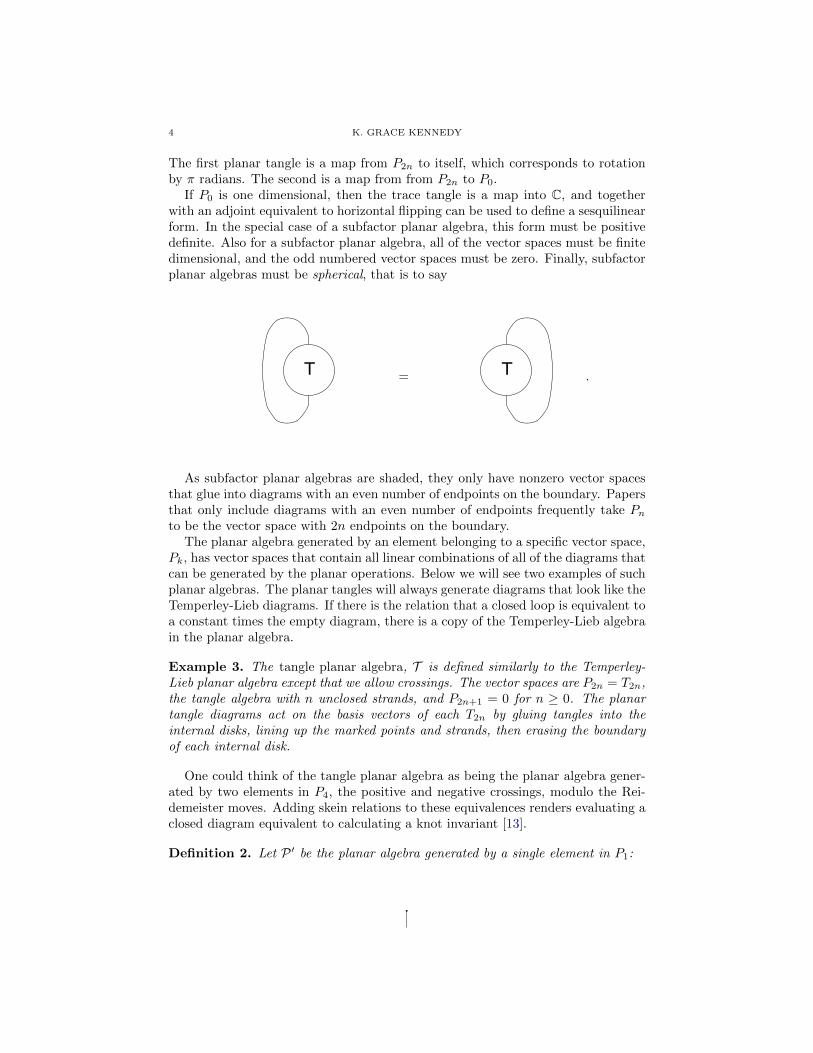
If P0 is one dimensional, then the trace tangle is a map into C, and togetherwith an adjoint equivalent to horizontal flipping can be used to define a sesquilinearform. In the special case of a subfactor planar algebra, this form must be positivedefinite. Also for a subfactor planar algebra, all of the vector spaces must be finitedimensional, and the odd numbered vector spaces must be zero. Finally, subfactorplanar algebras must be spherical, that is to say

T = T .

As subfactor planar algebras are shaded, they only have nonzero vector spacesthat glue into diagrams with an even number of endpoints on the boundary. Papersthat only include diagrams with an even number of endpoints frequently take Pnto be the vector space with 2n endpoints on the boundary.

The planar algebra generated by an element belonging to a specific vector space,Pk, has vector spaces that contain all linear combinations of all of the diagrams thatcan be generated by the planar operations. Below we will see two examples of suchplanar algebras. The planar tangles will always generate diagrams that look like theTemperley-Lieb diagrams. If there is the relation that a closed loop is equivalent toa constant times the empty diagram, there is a copy of the Temperley-Lieb algebrain the planar algebra.

Example 3. The tangle planar algebra, T is defined similarly to the Temperley-Lieb planar algebra except that we allow crossings. The vector spaces are P2n = T2n,the tangle algebra with n unclosed strands, and P2n+1 = 0 for n ≥ 0. The planartangle diagrams act on the basis vectors of each T2n by gluing tangles into theinternal disks, lining up the marked points and strands, then erasing the boundaryof each internal disk.

One could think of the tangle planar algebra as being the planar algebra gener-ated by two elements in P4, the positive and negative crossings, modulo the Rei-demeister moves. Adding skein relations to these equivalences renders evaluating aclosed diagram equivalent to calculating a knot invariant [13].

Definition 2. Let P ′ be the planar algebra generated by a single element in P1:

A DIAGRAMMATIC MULTIVARIATE ALEXANDER INVARIANT OF TANGLES 5

with relations in P0 and P4 respectively

= 0, = , and + = 0.

To ease notation, these relations make use of the definition of the dotted strand inDefinition 3 (below).

Definition 3. Define the dotted strand in P2 as

= − .

So the vector space Pk has basis vectors indexed by disks with k endpointson the boundary and strings with no crossings and one or two endpoints on theboundary. For the basis vectors, we require all strands with two endpoints on theboundary be dotted. Requiring that there be no dots gives another basis. Thevector spaces Pk are finite dimensional. Since a closed loop is equal to zero, P0 is 1-dimensional with every non-zero element equal to a multiple of the empty diagram.However, the inner product is not positive definite, and P1 being non-zero lets usknow immediately this is not a subfactor planar algebra.

The definition of the dotted strand is included to make the last relation lesscumbersome to write. It would otherwise include eight terms. This notation givesthe following two relations given in Bigelow’s Lemma 3.4 [5]:

Lemma 1. Where the internal dot is as in Definition 3, we have the following tworelations:

= 0

and

= .

The planar algebra P ′ was defined by Bigelow to give the diagrammatic algorithmfor the Alexander polynomial in [5]. It was also defined in Halverson and Benkart’s“Motzkin Algebras” in [4] and as a specific example of a planar algebra by Jonesin [12]. It has also come up in the theory of infinite index subfactors in the workof Jones and Penneys [11], [16], which we will briefly discuss in Section 6. In thefollowing section, we will outline how to send tangles into this planar algebra andretrieve the multivariate Alexander polynomial.

3. Algorithm and theorem

We will think of oriented knots and links as existing in the second vector spaceof the tangle planar algebra, the vector space of tangles with only one unclosedstrand. Each component has an orientation and is assigned a color, or variable.The knot or link we are considering is the one we get from making the obviousclosure.

6 K. GRACE KENNEDY

Figure 1.

q1

q2

q3

This is an example of a three-component link with colors q1, q2, and q3.

Definition 4. Let T be the set of oriented tangles written like elements in thetangle planar algebra with loose strands having endpoints on the boundary of a disk.Define ∆m : T→ P ′ to be the map from oriented tangles to P ′ that resolves positiveand negative crossings as follows:

qo qu= qo +qo +(qu−q−1u ) +q−1o −q−1o

qu qo= q−1o +q−1o −(qu−q−1u ) +qo −qo .

When we let the same variable be associated to every component then we haveLemmas 5.1-5.4 from [5]:

Lemma 2. The map ∆m on a knot or link where the same variable, q, is associatedto each component satisfies the skein relation

− = (q − q−1)

and all Reidemeister II and III moves and the following versions of ReidemeisterI:

= = −q−1

= = −q .

Lemma 2 tells us that up to a normalizing coefficient, the resolution of crossingsin Definition 4 is a single variable tangle invariant that satisfies the skein relationfor the Alexander polynomial. Restricting ourselves to oriented knots and links in

A DIAGRAMMATIC MULTIVARIATE ALEXANDER INVARIANT OF TANGLES 7

T2, the slight inconsistency with the first Reidemeister move can be dealt with bya simple normalizing coefficient. Define the turning number of a knot or link, T , tobe the number of positively oriented loops minus the number of negatively orientedloops denoted τ(T ). This brings us to Bigelow’s main result, Theorem 5.5 from [5].

Theorem 1. Where each strand has the same color, define

∆′(T ) = (−q)−τ(T )∆m(T ).

If T is an oriented tangle in T2, then ∆′(T ) is the Alexander polynomial of T̂ , theclosure of T .

The normalizing coefficient is a little more complicated for the multivariate ver-sion, but not much. The rotation number of a knot with color qi, denoted rot(qi),is the change in the angle in the counterclockwise direction when following a com-ponent in a link projection in the direction of the orientation divided by 2π.

Theorem 2. Define

∆′m : T2 −→ P2

T 7−→ N(T )∆m(T )

where N(T ) is the normalizing coefficient

N(T ) =( ∏

colors, qi

(−qi)−rot(qi))/

(ql − q−1l ),

and ql is the color of the strand with endpoints on the boundary of the disk. Thismap is the multivariate Alexander polynomial for a knot or link. Moreover, ∆m onhigher tangle vector spaces gives a tangle invariant up to Reidemeister I.

The subject of the next two sections will be proving Theorem 2. First in Section4 we must show that ∆′m respects the Reidemeister relations II and III exactly, andin T2, Reidemeister I is satisfied up to the given normalizing coefficient. Section 5will be dedicated to showing that this map on T2 satisfies the Murakami relations.

4. We do have a tangle invariant

In order to prove Theorem 2, we need to show that the Reidemeister movesare satisfied. Recall the resolutions that we must check satisfy the Reidemeisterrelations:

qo qu= qo +qo +(qu−q−1u ) +q−1o −q−1o

qu qo= q−1o +q−1o −(qu−q−1u ) +qo −qo .

Proof. Showing that these resolutions satisfy the given versions of Reidemeister Iinvolves only one strand, and this was covered in the proof in [5]. For ReidemeisterII and III, we must show all different versions since we are dealing with orientedlinks. This can be done by first showing two of the four versions of Reidemeister II,then two versions of Reidemeister III, and finally using these Reidemeister movesto check the remaining versions of Reidemeister II then III.

8 K. GRACE KENNEDY

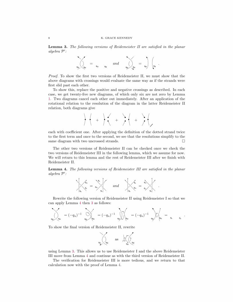
Lemma 3. The following versions of Reidemeister II are satisfied in the planaralgebra P ′:

qoqu

=qoqu

andqo qu

=qo qu

.

Proof. To show the first two versions of Reidemeister II, we must show that theabove diagrams with crossings would evaluate the same way as if the strands werefirst slid past each other.

To show this, replace the positive and negative crossings as described. In eachcase, we get twenty-five new diagrams, of which only six are not zero by Lemma1. Two diagrams cancel each other out immediately. After an application of therotational relation to the resolution of the diagram in the latter Reidemeister IIrelation, both diagrams give

+ + +

each with coefficient one. After applying the definition of the dotted strand twiceto the first term and once to the second, we see that the resolutions simplify to thesame diagram with two uncrossed strands. �

The other two versions of Reidemeister II can be checked once we check thetwo versions of Reidemeister III in the following lemma, which we assume for now.We will return to this lemma and the rest of Reidemeister III after we finish withReidemeister II.

Lemma 4. The following versions of Reidemeister III are satisfied in the planaralgebra P ′:

qo

qm

qu=

qo

qu

qm andqo

qm

qu

=qo

qm

qu.

Rewrite the following version of Reidemeister II using Reidemeister I so that wecan apply Lemma 4 then 3 as follows:

qo qu

= (−qu)−1

qo qu

= (−qu)−1qo qu

= (−qu)−1qo qu

=qo qu

.

To show the final version of Reidemeister II, rewrite

qoqu

asqoqu

using Lemma 3. This allows us to use Reidemeister I and the above ReidemeisterIII move from Lemma 4 and continue as with the third version of Reidemeister II.

The verification for Reidemeister III is more tedious, and we return to thatcalculation now with the proof of Lemma 4.

A DIAGRAMMATIC MULTIVARIATE ALEXANDER INVARIANT OF TANGLES 9

Proof. Resolving the crossings of the diagrams in the first version of ReidemeisterIII

qo

qm

quand

qo

qu

qm

gives a linear combination of 125 diagrams each. All but fifteen from both linearcombinations are zero. And these fifteen diagrams cancel each other out. The onlydiagrams with coefficients that require some verification to check that they cancelare

and .

The direct calculation of the other version of Reidemeister III is almost the same.There are only fifteen non-zero diagrams that all cancel. �

Any other version of the third Reidemeister move can be checked by applicationsof the second Reidemeister move so that any other version of Reidemeister III comesdown to the ones checked directly. For instance, rewrite this version of ReidemeisterIII in the following way:

qo

qm

qu=

qoqm

qu=

qoqm

qu.

Now one only has to apply the first Reidemeister III move from Lemma 4 and twoversions of Reidemeister II. �

5. The algorithm gives the multivariate Alexander polynomial

We will check that our algorithm gives the multivariate Alexander polynomialby checking the axioms from Murakami’s 1993 paper “A State Model for the Multi-variable Alexander Polynomial” [15]. All of the relations are straightforward exceptMurakami’s third relation, which is a relation in the algebra of colored braids withthree strands oriented upward. We will define this relation using colored versionsof σ1 and σ2 as positive generators and e is the “identity,” or three strands with nocrossings. In the braid group multiplication from left to right should be interpretedas stacking from top to bottom.

Definition 5. Murakami’s six axioms for a function ∆ on knots and links to bethe multivariate Alexander polynomial are:

(1) The single variable skein relation for two strands with the same color.(2)

(qaqb + q−1a q−1b )qbqa

=qa qb

+qa qb

(3) Define g+(x) = x + x−1 and g−(x) = x − x−1. From left to right alongthe bottom the colors of the strands in the algebra of colored braids are qa,qb, and qc. When we write ∆ of a braid in brackets, we mean ∆ of a link

10 K. GRACE KENNEDY

with that braid in it. Each of the links in this relation is exactly the sameeverywhere except for locally differing by these braids.

g+(qc)g−(qb)∆([σ1σ2σ2σ1])− g−(qb)g+(qa)∆([σ2σ1σ1σ2])−g−(q−1c qa)

[∆([σ1σ1σ2σ2]) + ∆([σ2σ2σ1σ1])

]+ g−(q−1c qbqa)g+(qa)∆([σ2σ2])

−g+(qc)g−(qcqbq−1a )∆([σ1σ1])− g−(q−2c q2a)∆([e])

= ZERO

(4) If L is the trivial knot with color qa, then ∆(L) = 1qa−q−1

a.

(5)

qa

qb

= (qa − q−1a )qa

(6) If L is the split union of a link and trivial knot, then ∆(L) is zero.

Proof. Note that Murakami’s axioms can be used to evaluate any 1-tangle in a disk.Indeed, one can rewrite the 1-tangle as an almost closed braid with only the standhaving endpoints on the boundary of the disk left unclosed. Murakami’s axiomsare independent of how one writes a link as the closure of a braid. The first threerelations can be used to reduce any link to a linear combination of disjoint unions ofconnected sums of Hopf links, and the remaining relations can be used to evaluatethese types of links [15].

These axioms are equally applicable to a 1-tangle written as an almost closedbraid. Indeed, the first three relations do not involve the portion of any strandconnecting the top of the braid to the bottom of the braid. Relations 4-6 can beapplied to any disjoint union of connected sums of Hopf links written as a 1-tangleto reduce the tangle to zero or a polynomial times the unclosed strand. So themultivariate Alexander polynomial of any 1-tangle is evaluable using Murakami’srelations, and the algorithm is independent of the choice of how to write the knotor link as a 1-tangle.

It is straightforward to check most of these relations. Relation 1 is the singlevariable skein relation shown by Bigelow [5]. Relation 4 is satisfied by the nor-malizing coefficient. Relation 6 comes directly from the first relation of the planaralgebra that a closed loop is zero. Relations 2 and 5 are no more difficult than thesecond Reidemeister move and can be checked by hand.

Proving Murakami’s third relation is significantly harder. We must define a rep-resentation on CB3, the algebra of colored braids with three strands. Let b be alinear combination of colored braids in CB3, and Lb will represent a linear combina-tion of knots or links that are identical everywhere except where they differ locallyaccording to b. We must define a representation, φ, so that φ(b) = 0 implies that∆′m(Lb) = 0. It might be worth noting a difference in convention here. Murakamihas all of his braids oriented downward, whereas ours are oriented upward. Wehope pointing this out directly will avoid some frustration over convention.

Definition 6. Let CB3 be the algebra of colored braids. That is to say braids whereeach strand has a color or label from {qa, qb, qc}. So there are now six versions ofσ1:

σ11 =

qa qb qc

, σ21 =

qaqbqc

, σ31 =

qaqb qc

, σ41 =

qaqb qc

, σ51 =

qa qbqc

, σ61 =

qa qbqc

.

A DIAGRAMMATIC MULTIVARIATE ALEXANDER INVARIANT OF TANGLES 11

The second generator follows the same conventions; σ12 is labeled qa, qb, and qc from

left to right across the bottom, σ22 is labeled qc, qb, qa, and so on.

Formally, you can stack any diagrams on top of one another, but the braid re-lations only exist for braids with a consistent coloring throughout the strand. Thisincludes the “identity,” e.

Let P6 be the sixth vector space of P ′. Define V to be the subspace of P6

generated by basis elements:

v1 = , v2 = , v3 = , v4 = ,

v5 = , v6 = , v7 = , v8 = .

The representation φ will be defined by resolving crossings of a braid in CB3 andsending it into P6 and then into M8(V,C). Call the map from CB3 into P6 thatresolves crossings, ρ. For all b ∈ CB3, ρ(vibvj) is equal to a coefficient, bi,j timesa single diagram. This is because with the given relations in P6, there is only oneway of connecting the strands of vi and vj by Lemma 1. The representation φ isdefined by:

(φ(b))i,j = bi,j .

Since bi,j = 0 if vi and vj have a different number of dotted strands also byLemma 1, the matrix φ(b) is a nice block matrix. The matrix for σ1

1 is

φ(σ11) =

qa 0 0 0 0 0 0 00 qb − q−1b q−1a 0 0 0 0 00 qa 0 0 0 0 0 00 0 0 qa 0 0 0 00 0 0 0 0 qa 0 00 0 0 0 q−1a qb − q−1b 0 00 0 0 0 0 0 −q−1a 00 0 0 0 0 0 0 −q−1a

.

All of the versions of σ1 are of the same form. Changing the coloring of the strandsonly permutes the variables. So the matrix φ(σ2

1) is

φ(σ21) =

qc 0 0 0 0 0 0 00 qb − q−1b q−1c 0 0 0 0 00 qc 0 0 0 0 0 00 0 0 qc 0 0 0 00 0 0 0 0 qc 0 00 0 0 0 q−1c qb − q−1b 0 00 0 0 0 0 0 −q−1c 00 0 0 0 0 0 0 −q−1c

.

The other versions of the generator σ2 are calculated in the same way, and σ12 ,

12 K. GRACE KENNEDY

which is labeled along the bottom with strands colored qa, qb, and qc, is

qb 0 0 0 0 0 0 00 qb 0 0 0 0 0 00 0 qc − q−1c q−1b 0 0 0 00 0 qb 0 0 0 0 00 0 0 0 −q−1b 0 0 00 0 0 0 0 0 qb 00 0 0 0 0 q−1b qc − q−1c 00 0 0 0 0 0 0 −q−1b

.

We must show (φ(uv))i,j = (φ(u)φ(v))i,j for u, v ∈ CB3. To do this, first notethat ρ(e) in P6 is equal to Σ8

k=1vk and v2k = vk for all k. Then the i, j entry ofφ(uv) is equal to the coefficient of viu(id)vvj = Σ8

k=1viuvkvvj = Σ8k=1viuv

2kvvj .

So (φ(uv))i,j = Σ8k=1(φ(u))i,k(φ(v))k,j , or the ith row of φ(u) dotted with the jth

column of φ(v), which is (φ(u)φ(v))i,j . So the proposed representation of CB3 ismultiplicative.

To finish showing that we have a representation of of CB3, we need to checkthe third Reidemeister move holds. In the uncolored braid group, this relation iswritten σ1σ2σ1 = σ2σ1σ2. We must make sure to use the appropriate versions ofthe generators so that the two braids have a consistent coloring along the strands.Labeling the bottom of the strands from left to right qa, qb, and qc, we must verifythat φ(σ3

1σ42σ

11) = φ(σ5

2σ61σ

12). Calculating the appropriate versions of σ1 and σ2,

the third Reidemeister move is easy to check in Mathematica. This shows that wehave a representation of the colored braid group.

Suppose Lb is a linear combination of knots or links that are identical exceptlocally where they differ by the terms in a linear combination of braids in CB3,b. Further suppose that φ(b) = 0. That ∆′m(Lb) = 0 follows from the fact ρ(e) =Σ8k=1vk:

∆′m(Lb) = ∆′m

bK

= ∆′m

bK

Σk=1vk8

= ∆′m(0) = 0 .

We have a representation of CB3 with the desired property. Checking Mu-rakami’s third relation is now an easy problem for Mathematica to do, and wesee that the representation of the linear combination of braids in Murakami’sthird relation is zero. I will include this Mathematica notebook on my websitehttp://www.math.ucsb.edu/∼kgracekennedy/. We have shown the Murakami re-lations hold and that we have an algorithm to calculate the multivariate Alexanderpolynomial of a link.

�

A DIAGRAMMATIC MULTIVARIATE ALEXANDER INVARIANT OF TANGLES 13

6. Conclusion

The resolutions of crossings defined in this paper give a new way to calculatethe multivariate Alexander polynomial of a link. The algorithm generalizes nicelyto a tangle invariant up to Reidemeister I. The tangle invariant is not a singlepolynomial but rather a linear combination of diagrams with coefficients that arepolynomials. There are several open questions about this invariant and the planaralgebra, such as is this the same tangle invariant as the one given by Archibaldin [3]. There is strong evidence to suggest that it is.

Anyone interested in planar algebras would probably like to know if this has anyrelation to subfactor theory. The planar algebra P ′ is not a subfactor planar algebra,but it is closely related to the Temperley-Lieb planar algebra. For example, if wetake a diagram in P ′ with no dots, we can “thicken” the strands. Broken strandsbecome shaded caps and cups, and through strands, or strands with one endpointon the top and one on the bottom, become two strands that bound a shaded region.For instance,

becomes

.

Diagrams with n boundary points on the top and bottom with only broken strandsand through strands form a subalgebra of the Temperley-Lieb algebra with nstrands [7]. These diagrams came up in the recent work of Jones and Penneyson infinite index subfactors. These subalgebras of the Temperley-Lieb algebrasalways appear injectively in the standard invariant of finite and infinite index sub-factors [11]. It is still unknown if there exists an infinite index subfactor for whichthe standard invariant is exactly these subalgebras [11], [16].

References

1. Samson Abramsky, Temperley-Lieb Algebra: From Knot Theory to Logic and Computationvia Quantum Mechanics, Quantum (2009), 45.

2. J. W. Alexander, Topological Invariants of Knots and Links, Transactions of the American

Mathematical Society 30 (1928), 275–306.3. Jana Archibald, The Multivariable Alexander Polynomial on Tangles, University of Toronto

Thesis (2010).4. Georgia Benkart and Tom Halverson, Motzkin Algebras, Arxiv preprint math/1106.5277

(2011).

5. Stephen Bigelow, A Diagrammatic Alexander Invariant of Tangles, Accepted for publicationat the Journal of Knot Theory and Its Ramifications.

6. Stephen Bigelow, Eric Ramos, and Ren Yi, The Alexander and Jones Polynomials Through

Representations of Rook Algebras, Arxiv preprint math/1110.0538v1 (2011).7. Alain Connes and David E. Evans, Embedding of U(1)-Current Algebras in Noncommutative

Algebras of Classical Statistical Mechanics, Comm. Math. Phys. 121 (1989), no. 3, 507–525.

MR 990778 (90k:46149)8. J H Conway, An Enumeration of Knots and Links, and Some of Their Algebraic Properties,

Computational Problems in Abstract Algebra Proc Conf Oxford 1967 329358 (1970), 329–

358.9. Daniel Flath, Tom Halverson, and Katheryn Herbig, The Planar Rook Algebra and Pascal’s

Triangle, L’Enseignement Mathmatique 55 (2009), 77–92.10. A Guionnet, V F R Jones, and D Shlyakhtenko, Random Matrices, Free Probability, Planar

Algebras and Subfactors, Elements (2007), 1–20.

14 K. GRACE KENNEDY

11. V F R Jones and David Penneys, Infinite Index Subfactors and the GICAR Algebras, http:

//math.berkeley.edu/~dpenneys/GICAR.pdf, 2011.

12. Vaughan F. R. Jones, Jones’s notes on planar algebras, http://math.berkeley.edu/~vfr/

VANDERBILT/pl21.pdf, 2011.

13. V.F.R. Jones, Planar Algebras, I, Arxiv preprint math/9909027 (1999).

14. Scott Morrison, Emily Peters, and Noah Snyder, Skein Theory for the D2n Planar Algebras,Journal of Pure and Applied Algebra 214 (2010), no. 2, 117–139.

15. Jun Murakami, A State Model for the Multi-variable Alexander Polynomial, Pacific Journal

of Mathematics 157 (1993), no. 1, 109–135.16. David Penneys, A Planar Calculus for Infinite Index Subfactors, Arxiv preprint

arXiv:1110.3504v1 (2011).

17. B. Westbury, The Representation Theory of the Temperley-Lieb Algebras, MathematischeZeitschrift 219 (1995), 539–565, 10.1007/BF02572380.

E-mail address: kgracekennedy@math.ucsb.edu