Embed Size (px)
Citation preview
Geometry & Topology 10 (2006) 1347–1372 1347arXiv version: fonts, pagination and layout may vary from GT published version
A dilogarithmic formulafor the Cheeger–Chern–Simons class
JOHAN L DUPONT
CHRISTIAN K ZICKERT
We present a simplification of Neumann’s formula for the universal Cheeger–Chern–Simons class of the second Chern polynomial. Our approach is completelyalgebraic, and the final formula can be applied directly on a homology class in thebar complex.
57M27; 57T30
Introduction
In the famous papers [1] and [2], J Cheeger, S Chern and J Simons define characteristicclasses for flat G–bundles. Each such characteristic class is given by a correspondinguniversal cohomology class in H∗(BGδ,C/Z), where δ denotes discrete topology.The cohomology of the classifying space of a discrete group is isomorphic to theEilenberg–Maclane group cohomology, and it has been a long standing problem to findexplicit formulas for the universal classes directly in terms of the bar complex. In [3],the first author proved that the universal Cheeger–Chern–Simons (C–C–S) class forthe group SL(2,C) associated to the second Chern polynomial is given up to a Q/Zindeterminacy by a dilogarithmic formula defined on the Bloch group B(C).
An element of B(C) is a formal sum of cross-ratios (see below), but the cross-ratio alonedoes not seem to carry enough information to get rid of the Q/Z indeterminacy on thereal part. Neumann [7] constructs an extended Bloch group B(C), where elements,in addition to the cross-ratio, also contain information of two choices of logarithms.It follows from Neumann’s article that this additional information is exactly what isneeded to remove the Q/Z indeterminacy. He shows that there is an isomorphism
λ : H3(PSL(2,C)) ∼= B(C),
and furthermore that there is a natural extension of the dilogarithmic formula from [3]to B(C) such that the composition of λ with the dilogarithm is exactly the universal
Published: 26 September 2006 DOI: 10.2140/gt.2006.10.1347
1348 Johan L Dupont and Christian K Zickert
C–C–S class. The formula also gives a combinatorial formula for the volume andthe Chern–Simons invariant of a complete hyperbolic manifold M with finite volume,since the C–C–S class evaluated on the canonical flat PSL(2,C)–bundle over M equalsi(Vol +iCS). This is shown by Neumann and Yang [8].
The isomorphism λ is defined by representing an element of H3(PSL(2,C)) by a“quasisimplicial complex,” and the appropriate choices of logarithms required to obtainan element in B(C) are found by studying combinatorial properties of this complex. Weconstruct a map similar to Neumann’s using SL(2,C) instead of PSL(2,C) and the moreextended Bloch group from [7, Section 8] instead of the extended Bloch group. We thusanswer affirmatively a question raised about the relation of this group to H3(SL(2,C))[7, page 443]. The definition of our map uses only simple homological algebra, and weobtain a formula which enables us to calculate the universal C–C–S class directly froma representative of a homology class in the bar complex. All geometry is replaced byalgebra which vastly simplifies the proofs.
We give a brief overview of the contents: In Section 1 we review the basic theory of theC–C–S classes, group homology and the Bloch group. Many details are included inorder to make the paper self-contained. In Section 2 we recall Neumann’s definitionof the (more) extended Bloch group. This overlaps with Neumann’s paper but for thesake of completeness, we include most of the details. In Section 3, we construct amap λ : H3(SL(2,C))→ B(C) by describing a way of detecting the appropriate twochoices of logarithms directly from a tuple of group elements. The idea is that the extrainformation can be found in C2\{0} rather than S2 using the Hopf map. In Section 4we show that our map actually calculates the C–C–S class and show that λ is surjectivewith kernel of order 2. Finally, we show in the appendix that our definition of theextended Bloch group agrees with that of Neumann.
Remark The reader should keep in mind that whenever we mention the extendedBloch group, we always mean the more extended Bloch group from [7, Section 8].Neumann uses the notation EB(C) for this group but we will use the notation B(C)even though this conflicts with the notation in [7].
Acknowledgements
This work was partially supported by The Danish Natural Science Research Council(Statens Naturvidenskabelige Forskningsrad), Denmark.
Geometry & Topology 10 (2006)
A dilogarithmic formula for the Cheeger–Chern–Simons class 1349
1 Preliminaries
In this section we review some basic theory and introduce our terminology. Throughout,F always denotes either R or C.
1.1 The Cheeger–Chern–Simons classes
We here recall some facts about the C–C–S classes that we shall need. For theirconstruction and basic properties, we refer to [1] or [2].
Let G be a Lie group with finitely many components and let Ik(G,F) denote the groupof invariant polynomials. Recall from classical Chern–Weil theory that there is a naturalhomomorphism
W : Ik(G,F)→ H2k(BG,F).
Let r denote the map H∗(BG,Z)→ H∗(BG,F) induced by the inclusion. The C–C–Sclasses are defined from the following data:
(1) An invariant polynomial P ∈ Ik(G,F).
(2) A class u ∈ H2k(BG,Z) satisfying W(P) = ru.
Let Kk(G,F) = {(P, u) ∈ Ik(G,F)× H2k(BG,Z) | W(P) = ru}.
Let Gδ denote the underlying discrete group of G. In [1] and [2], the authors describe away of associating a cohomology class P(u) in H2k−1(BGδ,F/Z) to an element (P, u)in Kk(G,F). This association is natural in the following sense:
Theorem 1.1 Let φ : G → H be a Lie group homomorphism between Lie groupswith finitely many components. The diagram below is commutative.
Kk(H,F)φ∗
//
C–C–S��
Kk(G,F)
C–C–S��
H2k−1(BHδ,F/Z)φ∗
// H2k−1(BGδ,F/Z)
Remark 1.2 In the following we shall only be interested in the C–C–S classescorresponding to the second Chern polynomial and the first Pontrjagin polynomial. Inboth cases u is just the corresponding Chern class or Pontrjagin class, and we simplydenote the associated C–C–S classes C2 and P1 .
Geometry & Topology 10 (2006)
1350 Johan L Dupont and Christian K Zickert
1.2 The homology of a group
Let G be a group. For a right G–module A, we let AG denote the group A ⊗Z[G] Z,where Z is regarded as a trivial G–module. The homology of G is by definition thehomology of the complex (P∗)G , where P∗ is a projective resolution of Z by rightG–modules. The following general construction of a projective resolution is of particularinterest to us: For X a set, let C∗(X) be the acyclic complex of free abelian groups,which in dimension n is generated by (n + 1)–tuples of elements in X . The differentialis given by
∂(x0, . . . , xn) =n∑
i=0
(−1)i(x0, . . . , xi, . . . , xn).
In particular for X = G, the diagonal left G–action on tuples makes C∗(G) into acomplex of G–modules (considered as right modules in the standard way) and C∗(G)augmented by the map C0(G)→ Z given by (g0) 7→ 1 is a free resolution of Z. Thecomplex C∗(G)G thus calculates the homology of G.
There is another description of this complex. Consider the complex B∗(G) of freeabelian groups, which in dimension n is generated by symbols [g1| · · · |gn] and withdifferential given by
∂[g1| · · · |gn] = [g2| · · · |gn] +n−1∑i=1
(−1)i[g1| · · · |gigi+1| · · · |gn]
+ (−1)n[g1| · · · |gn−1].
This complex is isomorphic to C∗(G)G via the map
(1–1) [g1| · · · |gn] 7→ (1, g1, g1g2, . . . , g1g2 · · · gn)
with inverse
(1–2) (g0, . . . , gn) 7→ [g−10 g1| · · · |g−1
n−1gn].
Hence, we can represent a homology class in Hn(G) either by a chain in Cn(G) or bya cycle in Bn(G). These two ways of representing homology classes are called thehomogenous and the inhomogenous representation, respectively.
Let M be a left G–module. The cohomology H∗(G,M) is defined as the homology ofthe complex HomZ[G](P∗,M), where P∗ , this time, is a projective resolution of Z byleft G–modules. Regarding a divisible abelian group A as a trivial G–module, we haveby the universal coefficient theorem a natural isomorphism
Hn(G,A) = Hom(Hn(G),A).
Geometry & Topology 10 (2006)
A dilogarithmic formula for the Cheeger–Chern–Simons class 1351
It is well known that the homology of a group is isomorphic to the singular homologyof its classifying space, and since the abelian group F/Z is obviously divisible, we canregard the C–C–S classes as homomorphisms from H3(G) to F/Z. It is an interestingproblem to try to find explicit formulas for the C–C–S classes directly in terms of theresolution C∗(G) (or some subcomplex). We shall investigate this in the followingsections.
We conclude the section with a little lemma that will be useful later. For each g ∈ Gthere is a map sg : C∗(G)→ C∗(G) given by sg(g0, . . . , gn) = (g, g0, . . . , gn).
Lemma 1.3 Let D∗(G) be a G–subcomplex of C∗(G). Suppose that for each cycle σin D∗(G), there exists a point g(σ) in G such that sg(σ)σ is in Dn+1(G). Then D∗(G) isacyclic and D∗(G)G calculates the homology of G.
Proof Note that ∂sg(g0, . . . , gn) = (g0, . . . , gn)− sg(∂(g0, . . . , gn)). Let σ be a cyclein D∗(G). Since ∂σ = 0 we have σ = ∂sg(σ)σ , that is, σ is a boundary.
1.3 The Bloch group
In all the following, we let G denote the group SL(2,C).
Definition 1.4 The pre-Bloch group P(C) is an abelian group generated by symbols[z], z ∈ C\{0, 1} subject to the relation
(1–3) [x]− [y] +[y
x
]−[1− x−1
1− y−1
]+[1− x
1− y
]= 0.
This relation is called the five term relation.
In [3] and [6] the five term relation is different, but this is because of the differentdefinition of the cross-ratio (1–4).
Definition 1.5 The Bloch group B(C) is the kernel of the homomorphism
ν : P(C)→ C∗ ∧ C∗
to the second exterior power of the abelian group C∗ defined by mapping a generator[z] to z ∧ (1− z).
Geometry & Topology 10 (2006)
1352 Johan L Dupont and Christian K Zickert
There is an important interpretation of the pre-Bloch group in terms of a homologygroup. Recall the notation from Section 1.2. Let C 6=∗ (S2) denote the subcomplex ofC∗(S2) consisting of tuples of distinct elements. Recall that G = SL(2,C) acts onS2 = C ∪ {∞} by Mobius transformations, that is,(
a bc d
)z =
az + bcz + d
.
Via this action, the complex C 6=∗ (S2) becomes a complex of G–modules. The action is3–transitive and four distinct points z0, . . . , z3 are determined up to the action by thecross-ratio
(1–4) z = [z0 : z1 : z2 : z3] :=(z0 − z3)(z1 − z2)(z0 − z2)(z1 − z3)
.
Note that in [3] and [6] the cross-ratio is defined to be the reciprocal of (1–4). It followsthat C 6=3 (S2)G is just the free abelian group on C\{0, 1}. One easily checks that thefive term relation is equivalent to the relation
4∑i=0
(−1)i[z0 : · · · : zi : · · · : z4] = 0.
This means that the kernel of the cross-ratio map σ : C 6=3 (S2)→ P(C) is exactly theboundaries. Since C 6=2 (S2)G = Z by 3–transitivity, C 6=3 (S2)G consists entirely of cycles,and σ induces an isomorphism
σ : H3(C 6=∗ (S2)G)→ P(C).
We have the following relations in the pre-Bloch group [6, Lemma 5.11]:
[x] =[ 1
1− x
]=[1− 1
x
]= −
[1x
]= −
[ xx− 1
]= −[1− x]
If we extend the cross-ratio by setting [z0 : z1 : z2 : z3] = 0 if there are equals amongz0, . . . , z3 , it follows from the above relations that σ can be extended to H3(C∗(S2)G).We omit the details. We can now define a map
λ : H3(G)→ P(C)
as the composition
H3(G) // H3(C∗(S2)G)σ // P(C)
where the left map is induced by
C3(G)→ C3(S2), (g0, . . . , g3) 7→ (g0∞, g1∞, g2∞, g3∞).
Geometry & Topology 10 (2006)
A dilogarithmic formula for the Cheeger–Chern–Simons class 1353
In [6] it is shown that λ has image in the Bloch group and that the following sequence,which is essentially due to Bloch and Wigner, is exact.
(1–5) 0 // Q/Z // H3(G) λ // B(C) // 0
Using the isomorphism Q/Z = lim−→Z/nZ = lim−→H3(Z/nZ), the left map is the limitmap induced by the maps Z/nZ→ G given by sending 1 to the matrix of a rotation by2π/n.
1.4 Rogers’ dilogarithm
We here review a result in [3] relating the C–C–S class P1 to a dilogarithm function viathe Bloch group.
Rogers’ dilogarithm is the following function defined on the open interval (0, 1):
(1–6) L(z) = −12
Log(z) Log( 1
1− z
)+ Li2(z)− π2
6Here Li2(z) = −
∫ z0
Log(1−t)t dt is the classical dilogarithm function. As in [9] we have
subtracted π2/6 from the original Rogers’ dilogarithm in order to make it satisfy (1–8).L is real analytic and satisfies the functional equations
L(x) + L(1− x) = −π2
6(1–7)
L(x)− L(y) + L(y
x
)− L(1− x−1
1− y−1
)+ L(1− x
1− y
)= 0, y < x.(1–8)
We can extend L (discontinuously) to R by setting
L(1) = 0, L(0) = −π2
6and L(x) =
{−L(1/x) for x > 1
−L(x/(x− 1)) for x < 0
and define a map L : C3(SL(2,R))→ R by
(1–9) (g0, . . . , g3)→ L([g0∞ : · · · : g3∞]).
This is clearly well-defined (recall that cross-ratios are defined to be zero when thereare equals) since all cross-ratios are real. Also, a few calculations using the functionalequations show that the map takes boundaries to multiples of π2/6, that is, it is a3–cocycle modulo π2/6. The theorem below can be found in [3]. The minus sign thereis due to the differing definition of the cross-ratio.
Theorem 1.6 14π2 L equals the Cheeger–Chern–Simons class P1 modulo 1/24.
Geometry & Topology 10 (2006)
1354 Johan L Dupont and Christian K Zickert
Since the restriction of the second Chern polynomial to the Lie algebra of SL(2,R)is minus the Pontrjagin polynomial, it follows from Theorem 1.1 that we have acommutative diagram:
(1–10)
H3(SL(2,R))−bP1 //
��
R/Z
��
H3(SL(2,C))bC2 // C/Z
By Theorem 1.6, P1 is (modulo 1/24) just a dilogarithm via the Bloch group. We wishto find a similar expression for C2 by extending L to H3(SL(2,C)). This is partiallysolved in [3] by studying a homomorphism c : B(C) → C/Q, known as the Blochregulator, and showing that the composition below is 2C2 .
H3(SL(2,C)) λ // B(C) c // C/Q
We shall improve this by showing that there is a commutative diagram
H3(SL(2,C))bλ //
��
B(C)− 1
2π2bL
//
��
C/Z
��
H3(SL(2,C))/(Q/Z) λ // B(C) c // C/Q
so that the top composition is 2C2 . Here B(C) is Neumann’s extended Bloch group(see [7] or Section 2). In other words, C2 is a dilogarithm via the extended Bloch groupexactly as P1 is a dilogarithm via the Bloch group.
2 The extended Bloch group
In this section we review Neumann’s definition of the extended Bloch group. Asmentioned in the introduction the reader should keep in mind that our extended Blochgroup is what Neumann calls the more extended Bloch group.
We shall use the conventions that the argument Arg z of a complex number alwaysdenotes the main argument (−π < Arg z ≤ π ) and the logarithm Log z always denotesthe logarithm having Arg z as imaginary part.
The idea is to construct a Riemann surface C covering C\{0, 1} and then construct theextended pre-Bloch group P(C) as in Definition 1.4, with an appropriate lift of the fiveterm relation.
Geometry & Topology 10 (2006)
A dilogarithmic formula for the Cheeger–Chern–Simons class 1355
Let C denote the universal abelian cover of C\{0, 1}. There is a nice way of representingpoints in C. Let Ccut denote C\{0, 1} cut open along each of the intervals (−∞, 0)and (1,∞) so that each real number r outside of [0, 1] occurs twice in Ccut . We shalldenote these two occurrences of r by r + 0i and r − 0i respectively. It is now easy tosee that C is isomorphic to the surface obtained from Ccut × 2Z× 2Z by the followingidentifications:
(x + 0i, 2p, 2q) ∼ (x− 0i, 2p + 2, 2q) for x ∈ (−∞, 0)
(x + 0i, 2p, 2q) ∼ (x− 0i, 2p, 2q + 2) for x ∈ (1,∞).
This means that points in C are of the form (z, p, q) with z ∈ C\{0, 1} and p, q evenintegers. Note that C can be regarded as the Riemann surface for the function
C\{0, 1} → C2, z 7→(
Log z,Log( 1
1− z
)).
We shall show below that L can be extended holomorphically to be defined on C, andthen we shall simply define the extended five term relation to be the smallest possibleextension of the relation (1–8).
Consider the set
FT :={(
x, y,yx,
1− x−1
1− y−1 ,1− x1− y
)}⊂ (C\{0, 1})5
of five-tuples involved in the five term relation. Also let
FT0 = {(x0, . . . , x4) ∈ FT | 0 < x1 < x0 < 1}
be the set of five-tuples involved in the functional equation (1–8). Define the setFT ⊂ C× · · · × C to be the component of the preimage of FT that contains all points((x0; 0, 0), . . . , (x4; 0, 0)
)with (x0, . . . , x4) ∈ FT0 .
Remark 2.1 This notation conflicts with the notation in [7]. Our FT is what Neumanncalls FT00 in [7, Section 8]. This is shown in the appendix.
Definition 2.2 The extended pre-Bloch group P(C) is the abelian group generated bysymbols [z; p, q], with (z; p, q) ∈ C, subject to the relation
4∑i=0
(−1)i[xi; pi, qi] = 0 for ((x0; p0, q0), . . . , (x4; p4, q4)) ∈ FT.
This relation is called the extended five term relation.
Geometry & Topology 10 (2006)
1356 Johan L Dupont and Christian K Zickert
Definition 2.3 The extended Bloch group B(C) is the kernel of the homomorphism(which is well-defined by [7, Lemma 2.3])
ν : P(C)→ C ∧ C
defined on generators by [z; p, q] 7→ (Log z + pπi) ∧ (−Log(1− z) + qπi).
We now extend L to C. First note that the expression in (1–6) is well-defined for allz ∈ C\{0, 1}, and that L extended this way is holomorphic except at real points outsidethe interval between 0 and 1.
Define L(z; p, q) = L(z) +πi2
(q Log(z)− p Log
( 11− z
)).
Remark 2.4 Neumann calls this map R (probably for Rogers), but in fact Rogersoriginally called his dilogarithm L. Also, the name L is more consistent with ourconvention that all extended groups and maps be labelled with a hat.
Proposition 2.5 (Neumann [7, Proposition 2.5]) 12π2 L gives a well-defined and
holomorphic map C → C/Z. Also the extended five term relation is a functionalequation so that 1
2π2 L gives a homomorphism P(C)→ C/Z.
2.1 Geometry of the extended pre-Bloch group
We first recall some geometric properties of the cross-ratio. Let z0, z1, z2, z3 be fourdistinct ordered points in C ∪ {∞}. Regarding C ∪ {∞} as the boundary of thestandard compactification of hyperbolic 3–space H3 , the four points define a uniqueideal hyperbolic simplex [z0, . . . , z3] which is determined up to orientation preservingcongruence by the cross-ratio
(2–1) z = [z0 : z1 : z2 : z3] :=(z0 − z3)(z1 − z2)(z0 − z2)(z1 − z3)
.
Clearly z ∈ C\{0, 1} and since [0 :∞ : 1 : z] = z, every z ∈ C\{0, 1} can be realizedas the cross-ratio of an ideal hyperbolic simplex. It is well known that z is real if andonly if the four points lie on a circle (that is circle or straight line) and in this case thesimplex is called flat.
We orient H3 such that the cross-ratio of a nonflat simplex has positive imaginary partif and only if the orientation induced by the vertex ordering agrees with the orientationinherited from H3 . There is a nice geometric interpretation of the argument of z. Ifthe imaginary part of z is greater than or equal to zero then Arg z is the dihedral angle
Geometry & Topology 10 (2006)
A dilogarithmic formula for the Cheeger–Chern–Simons class 1357
of the simplex corresponding to the edge [z0z1]. Otherwise, that is if the orientationdisagrees with the orientation of H3 , it is minus the dihedral angle.
It easily follows from (2–1) that an even permutation of the zi ’s replaces z by one ofthree so-called cross-ratio parameters:
z, z′ =1
1− zand z′′ = 1− 1
z
In particular the dihedral angle corresponding to the edges [z1z2] and [z1z3] are Arg(z′)and Arg(z′′) respectively, (or their negatives if the vertex ordering does not agree withthe orientation of H3 ). Since a product of two disjoint transpositions clearly keeps thecross-ratio fixed, we see that the dihedral angles of opposite edges are the same. Notethat since zz′z′′ = −1 the sum of the dihedral angles is always π . This is not surprisingsince a horosphere at an ideal vertex of a hyperbolic simplex intersects the simplex in aEuclidean triangle.
Definition 2.6 A combinatorial flattening of an ideal simplex with cross-ratio z is atriple (w0,w1,w2) of complex numbers with w0 + w1 + w2 = 0, where w0 and w1 arechoices of logarithms of z and z′ . We call w0,w1 and w2 log-parameters.
Note that w2 ± πi is a choice of logarithm of z′′ . The set of combinatorial flatteningsof ideal simplices is in bijective correspondence with C by the map l given by
(2–2) l(w0,w1,w2) =(
z;w0 − Log z
πi,
w1 − Log( 11−z )
πi
)where z = ew0 . This means that the extended pre-Bloch group can be regarded as beinggenerated by combinatorial flattenings of ideal simplices, whereas the pre-Bloch groupcan be regarded as being generated by congruence classes of ideal simplices. Let usdiscuss the five term relation in this geometric setup.
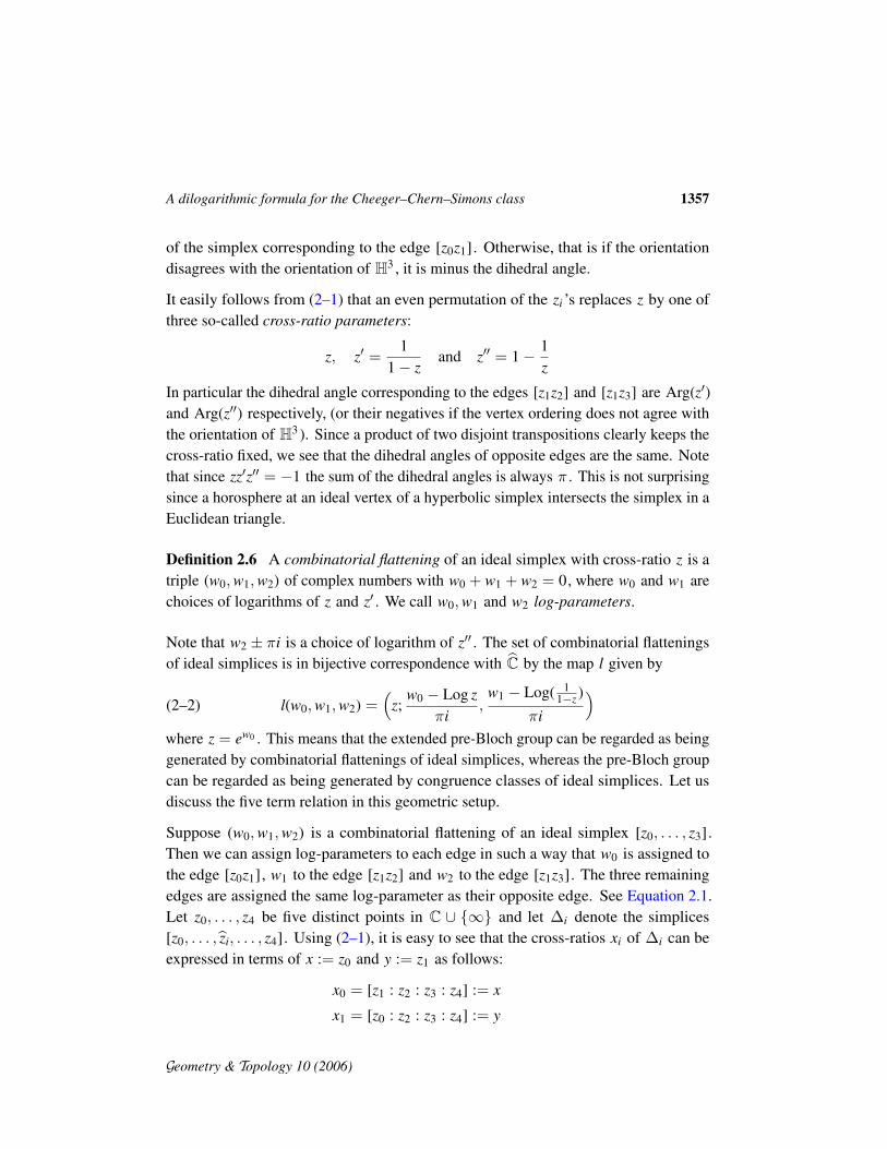
Suppose (w0,w1,w2) is a combinatorial flattening of an ideal simplex [z0, . . . , z3].Then we can assign log-parameters to each edge in such a way that w0 is assigned tothe edge [z0z1], w1 to the edge [z1z2] and w2 to the edge [z1z3]. The three remainingedges are assigned the same log-parameter as their opposite edge. See Equation 2.1.Let z0, . . . , z4 be five distinct points in C ∪ {∞} and let ∆i denote the simplices[z0, . . . , zi, . . . , z4]. Using (2–1), it is easy to see that the cross-ratios xi of ∆i can beexpressed in terms of x := z0 and y := z1 as follows:
x0 = [z1 : z2 : z3 : z4] := x
x1 = [z0 : z2 : z3 : z4] := y
Geometry & Topology 10 (2006)
1358 Johan L Dupont and Christian K Zickert
x2 = [z0 : z1 : z3 : z4] =yx
x3 = [z0 : z1 : z2 : z4] =1− x−1
1− y−1
x4 = [z0 : z1 : z2 : z3] =1− x1− y
z0 z1
z2z3 w0
w0
w1 w1
w2w2
Figure 1: Assignment of log-parameters to edges of an ideal simplex
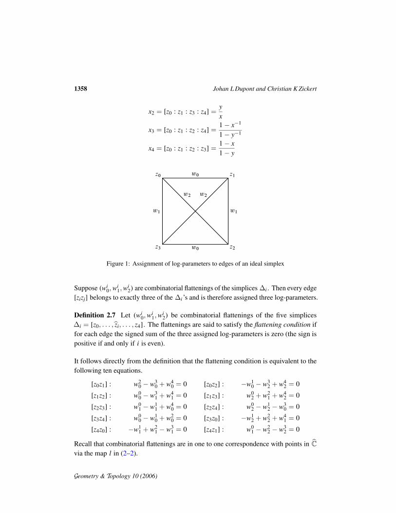
Suppose (wi0,w
i1,w
i2) are combinatorial flattenings of the simplices ∆i . Then every edge
[zizj] belongs to exactly three of the ∆i ’s and is therefore assigned three log-parameters.
Definition 2.7 Let (wi0,w
i1,w
i2) be combinatorial flattenings of the five simplices
∆i = [z0, . . . , zi, . . . , z4]. The flattenings are said to satisfy the flattening condition iffor each edge the signed sum of the three assigned log-parameters is zero (the sign ispositive if and only if i is even).
It follows directly from the definition that the flattening condition is equivalent to thefollowing ten equations.
[z0z1] : w20 − w3
0 + w40 = 0 [z0z2] : −w1
0 − w32 + w4
2 = 0
[z1z2] : w00 − w3
1 + w41 = 0 [z1z3] : w0
2 + w21 + w4
2 = 0
[z2z3] : w01 − w1
1 + w40 = 0 [z2z4] : w0
2 − w12 − w3
0 = 0
[z3z4] : w00 − w1
0 + w20 = 0 [z3z0] : −w1
2 + w22 + w4
1 = 0
[z4z0] : −w11 + w2
1 − w31 = 0 [z4z1] : w0
1 − w22 − w3
2 = 0
Recall that combinatorial flattenings are in one to one correspondence with points in Cvia the map l in (2–2).
Geometry & Topology 10 (2006)
A dilogarithmic formula for the Cheeger–Chern–Simons class 1359
Theorem 2.8 (Neumann [7, Lemma 3.4]) Flattenings (wi0,w
i1,w
i2) satisfy the flatten-
ing condition if and only if∑4
i=0(−1)i[l(wi0,w
i1,w
i2)] = 0 in P(C).
This means that the flattening condition is equivalent to the extended five term relation.
3 Mappings via configurations in C2\{0}
In this section we explore the idea that the extra information needed to remove theQ/Z indeterminacy in Dupont’s formula for the C–C–S class C2 can be detected byconfigurations in C2\{0} instead of S2 . Let h denote the Hopf map h : C2\{0} →S2 = C ∪ {∞} given by
(z,w) 7→ z/w.
We will show that for certain tuples (v0, . . . , v3) of points in C2\{0}, there is a naturalchoice of combinatorial flattening of the ideal simplex [hv0, . . . , hv3]. This means thatsuch a tuple gives an element in P(C). We also describe a way of associating such atuple to a tuple of group elements in such a way that we obtain a map
λ : H3(G)→ P(C).
Recall from Section 1.3 that there is a map σ : C 6=3 (S2)G → P(C). We saw thatboundaries were mapped to zero and that the induced map
σ : H3(C 6=∗ (S2)G)→ P(C)
is an isomorphism. We shall elaborate on this and construct a G–complex Ch6=∗ (C2)
and a map σ : Ch6=3 (C2)G → P(C) giving rise to a commutative diagram:
H3(Ch6=∗ (C2)G)
bσ //
h��
P(C)
��
H3(C 6=∗ (S2)G)σ // P(C)
We define the complex Ch6=∗ (C2) as the subcomplex of C∗(C2\{0}) consisting of tuples
mapping to different elements in S2 by the Hopf map h. The G–module structure isgiven by the natural G–action on C2\{0}, and since this action is h–equivariant, hinduces a G–map Ch6=
∗ (C2)→ C 6=∗ (S2) and hence a map
h : H3(Ch6=∗ (C2)G)→ H3(C 6=∗ (S2)G).
Geometry & Topology 10 (2006)
1360 Johan L Dupont and Christian K Zickert
3.1 Mapping to the extended pre-Bloch group
We now assign to each 4–tuple (v0, v1, v2, v3) ∈ Ch6=3 (C2) a combinatorial flattening of
the ideal simplex [hv0, hv1, hv2, hv3] in such a way that the combinatorial flatteningsassigned to tuples (v0, . . . , vi, . . . v4) satisfy the flattening condition. This will give us amap
σ : H3(Ch6=∗ (C2)G)→ P(C).
The key step is to observe that the cross-ratio parameters z and 11−z of a simplex
[hv0, hv1, hv2, hv3] can be expressed in terms of determinants
z := [hv0 : hv1 : hv2 : hv3] =
(v1
0v2
0− v1
3v2
3
)(
v10
v20− v1
2v2
2
)(
v11
v21− v1
2v2
2
)(
v11
v21− v1
3v2
3
) =det(v0, v3) det(v1, v2)det(v0, v2) det(v1, v3)
where the upper indices refer to first or second coordinate in C2 . Similarly,
11− z
= [hv0 : hv2 : hv0 : hv3] =
(v1
1v2
1− v1
3v2
3
)(
v11
v21− v1
0v2
0
)(
v12
v22− v1
0v2
0
)(
v12
v22− v1
3v2
3
) =det(v1, v3) det(v0, v2)det(v0, v1) det(v2, v3)
.
Since obviously hvi 6= hvj if and only if det(vi, vj) 6= 0, all these determinants arenonzero. This suggests that we can assign a flattening to (v0, v1, v2, v3) by setting
w0 = Log det(v0, v3) + Log det(v1, v2)− Log det(v0, v2)− Log det(v1, v3)
w1 = Log det(v0, v2) + Log det(v1, v3)− Log det(v0, v1)− Log det(v2, v3)
w2 = Log det(v0, v1) + Log det(v2, v3)− Log det(v0, v3)− Log det(v1, v2).
This defines a map σ : Ch6=3 (C2)→ P(C) by
(3–1) (v0, v1, v2, v3) 7→ [l(w0,w1,w2)].
Now suppose (w00,w
01,w
02), . . . , (w4
0,w41,w
42) are flattenings defined as above of simplices
[hv0, . . . , hvi, . . . , hv4]. We must check that these flattenings satisfy the flatteningcondition. This is equivalent to checking that all the ten equations listed belowDefinition 2.7 are satisfied. We check the first of these and leave the others to the reader.Using the notation (v,w) := Log det(v,w) we have
Geometry & Topology 10 (2006)
A dilogarithmic formula for the Cheeger–Chern–Simons class 1361
w20 = (v0, v4) + (v1, v3)− (v0, v3)− (v1, v4)
w30 = (v0, v4) + (v1, v2)− (v0, v2)− (v1, v4)
w40 = (v0, v3) + (v1, v2)− (v0, v2)− (v1, v3)
from which it follows that the equation w20 − w3
0 + w40 = 0 is satisfied.
Having verified all the ten equations, it now follows from Theorem 2.8 that σ sendsboundaries to zero. Since σ obviously factors through Ch6=
3 (C2)G , we obtain a mapσ : H3(Ch6=
∗ (C2)G)→ P(C).
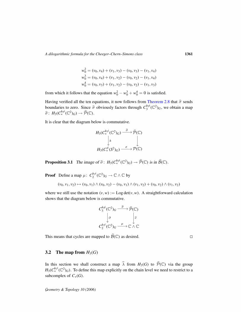
It is clear that the diagram below is commutative.
H3(Ch6=∗ (C2)G)
bσ //
h��
P(C)
��
H3(C 6=∗ (S2)G)σ // P(C)
Proposition 3.1 The image of σ : H3(Ch6=∗ (C2)G)→ P(C) is in B(C).
Proof Define a map µ : Ch6=2 (C2)G → C ∧ C by
(v0, v1, v2) 7→ (v0, v1) ∧ (v0, v2)− (v0, v1) ∧ (v1, v2) + (v0, v2) ∧ (v1, v2)
where we still use the notation (v,w) := Log det(v,w). A straightforward calculationshows that the diagram below is commutative.
Ch6=3 (C2)G
bσ //
∂��
P(C)
b�
Ch6=2 (C2)G
µ// C ∧ C
This means that cycles are mapped to B(C) as desired.
3.2 The map from H3(G)
In this section we shall construct a map λ from H3(G) to P(C) via the groupH3(Ch6=
∗ (C2)G). To define this map explicitly on the chain level we need to restrict to asubcomplex of C∗(G).
Geometry & Topology 10 (2006)
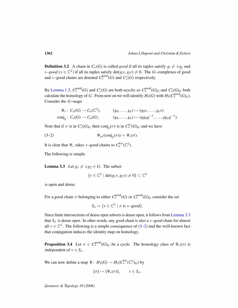
1362 Johan L Dupont and Christian K Zickert
Definition 3.2 A chain in C∗(G) is called good if all its tuples satisfy gi 6= ±gj andv–good (v ∈ C2 ) if all its tuples satisfy det(giv, gjv) 6= 0. The G–complexes of goodand v–good chains are denoted Cgood
∗ (G) and Cv∗(G) respectively.
By Lemma 1.3, Cgood∗ (G) and Cv
∗(G) are both acyclic so Cgood∗ (G)G and Cv
∗(G)G bothcalculate the homology of G. From now on we will identify H3(G) with H3(Cgood
∗ (G)G).Consider the G–maps
Ψv : Cn(G)→ Cn(C2), (g0, . . . , gn) 7→ (g0v, . . . , gnv)
conjg : Cn(G)→ Cn(G), (g0, . . . , gn) 7→ (gg0g−1, . . . , ggng−1).
Note that if σ is in Cv∗(G)G then conjg(σ) is in Cgv
∗ (G)G and we have
(3–2) Ψgv(conjg(σ)) = Ψv(σ).
It is clear that Ψv takes v–good chains to Ch6=n (C2).
The following is simple.
Lemma 3.3 Let g1 6= ±g2 ∈ G. The subset
{v ∈ C2 | det(g1v, g2v) 6= 0} ⊂ C2
is open and dense.
For a good chain σ belonging to either Cgood∗ (G) or Cgood
∗ (G)G consider the set
Sσ = {v ∈ C2 | σ is v–good}.
Since finite intersections of dense open subsets is dense open, it follows from Lemma 3.3that Sσ is dense open. In other words, any good chain is also a v–good chain for almostall v ∈ C2 . The following is a simple consequence of (3–2) and the well-known factthat conjugation induces the identity map on homology.
Proposition 3.4 Let σ ∈ Cgood∗ (G)G be a cycle. The homology class of Ψv(σ) is
independent of v ∈ Sσ .
We can now define a map Ψ : H3(G)→ H3(Ch6=∗ (C2)G) by
[σ] 7→ [Ψv(σ)], v ∈ Sσ.
Geometry & Topology 10 (2006)
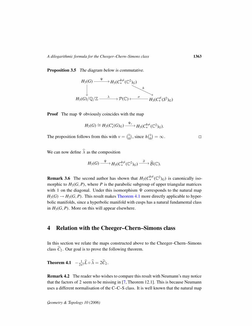
A dilogarithmic formula for the Cheeger–Chern–Simons class 1363
Proposition 3.5 The diagram below is commutative.
H3(G) Ψ //
��
H3(Ch6=∗ (C2)G)
h
''PPPPPPPPPPPP
H3(G)/Q/Z λ // P(C) H3(C 6=∗ (S2)G)σoo
Proof The map Ψ obviously coincides with the map
H3(G) ∼= H3(Cv∗(G)G) Ψv // H3(Ch6=
∗ (C2)G).
The proposition follows from this with v =(1
0
), since h
(10
)=∞.
We can now define λ as the composition
H3(G) Ψ // H3(Ch6=∗ (C2)G)
bσ // B(C).
Remark 3.6 The second author has shown that H3(Ch6=∗ (C2)G) is canonically iso-
morphic to H3(G,P), where P is the parabolic subgroup of upper triangular matriceswith 1 on the diagonal. Under this isomorphism Ψ corresponds to the natural mapH3(G)→ H3(G,P). This result makes Theorem 4.1 more directly applicable to hyper-bolic manifolds, since a hyperbolic manifold with cusps has a natural fundamental classin H3(G,P). More on this will appear elsewhere.
4 Relation with the Cheeger–Chern–Simons class
In this section we relate the maps constructed above to the Cheeger–Chern–Simonsclass C2 . Our goal is to prove the following theorem.
Theorem 4.1 − 12π2 L ◦ λ = 2C2 .
Remark 4.2 The reader who wishes to compare this result with Neumann’s may noticethat the factors of 2 seem to be missing in [7, Theorem 12.1]. This is because Neumannuses a different normalisation of the C–C–S class. It is well known that the natural map
Geometry & Topology 10 (2006)
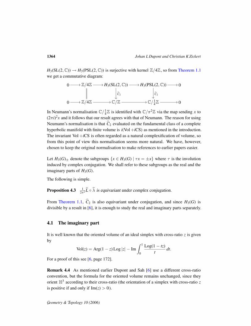
1364 Johan L Dupont and Christian K Zickert
H3(SL(2,C))→ H3(PSL(2,C)) is surjective with kernel Z/4Z, so from Theorem 1.1we get a commutative diagram:
0 // Z/4Z // H3(SL(2,C))
bC2��
// H3(PSL(2,C))
bC2��
// 0
0 // Z/4Z // C/Z // C/14Z // 0
In Neumann’s normalisation C/14Z is identified with C/π2Z via the map sending x to
(2πi)2x and it follows that our result agrees with that of Neumann. The reason for usingNeumann’s normalisation is that C2 evaluated on the fundamental class of a completehyperbolic manifold with finite volume is i(Vol +iCS) as mentioned in the introduction.The invariant Vol +iCS is often regarded as a natural complexification of volume, sofrom this point of view this normalisation seems more natural. We have, however,chosen to keep the original normalisation to make references to earlier papers easier.
Let H3(G)± denote the subgroups {x ∈ H3(G) | τx = ±x} where τ is the involutioninduced by complex conjugation. We shall refer to these subgroups as the real and theimaginary parts of H3(G).
The following is simple.
Proposition 4.3 12π2 L ◦ λ is equivariant under complex conjugation.
From Theorem 1.1, C2 is also equivariant under conjugation, and since H3(G) isdivisible by a result in [6], it is enough to study the real and imaginary parts separately.
4.1 The imaginary part
It is well known that the oriented volume of an ideal simplex with cross-ratio z is givenby
Vol(z) = Arg(1− z) Log |z| − Im∫ 1
0
Log(1− tz)t
dt.
For a proof of this see [6, page 172].
Remark 4.4 As mentioned earlier Dupont and Sah [6] use a different cross-ratioconvention, but the formula for the oriented volume remains unchanged, since theyorient H3 according to their cross-ratio (the orientation of a simplex with cross-ratio zis positive if and only if Im(z) > 0).
Geometry & Topology 10 (2006)
A dilogarithmic formula for the Cheeger–Chern–Simons class 1365
The five term relation (1–3) is easily seen to be a functional equation for Vol. Thismeans that Vol is well-defined on the pre-Bloch group and therefore also on the extendedpre-Bloch group.
Theorem 4.5 (Dupont [3, Proposition 3.1]) Im C2 = − 14π2 Vol ◦λ.
Proposition 4.6 The restriction of Im L : P(C)→ R to B(C) equals Vol.
Proof Let τ =∑
(−1)εi[zi; pi, qi] ∈ B(C). Since
Im L([z; p, q]) =12(
Arg(z) Log |1− z|+ Log |z|Arg(1− z))
− Im∫ 1
0
Log(1− tz)t
dt +π
2p Log |1− z|+ π
2q Log |z|
Vol(z)− ImL([z; p, q]) =12(
Log |z|Arg(1− z)− Arg(z) Log |1− z|)
we have
− π
2p Log |1− z| − π
2q Log |z|.
Let φ denote the composition
C ∧ C = (R ∧ R)⊕ (iR ∧ iR)⊕ (R⊗ iR)→ R⊗ iR→ iR
where the left map is projection and the right map is multiplication. A simple calculationshows that
φ(ν([z; p, q])
)= −i Log |z|Arg(1− z) + i Arg(z) Log |1− z|
+ pπi Log |1− z|+ qπi Log |z| = −2i(
Vol(z)− Im L([z; p, q])).
Since ν(τ ) = 0, we have Vol(τ ) = Im L(τ ) as desired.
4.2 The real part
Let GR = SL(2,R). The key step is the following theorem of Dupont, Parry and Sah[5, 10].
Theorem 4.7 The inclusion GR → G induces an isomorphism
H3(GR) ∼= H3(G)+.
Geometry & Topology 10 (2006)

1366 Johan L Dupont and Christian K Zickert
This means that it is enough to study real cycles. The idea is that every homology classin H3(GR) has a representative such that the image of L ◦ λ is the same as the image ofthe cocycle L from (1–9).
In the following the reader should bear in mind the relationship between the homogenousand the inhomogenous representations of cycles given by the equations (1–1) and (1–2).
Definition 4.8 An element(
a bc d
)∈ GR is called positive if c is positive and nonzero if
c is nonzero. A chain in Bn(GR) is called positive if all its group elements are positive.
If (g1, g2, g3) is a triple of positive elements that are so small (close to the identity) thatalso g1g2 , g2g3 and g1g2g3 are positive, we have
• (v0, v1, v2, v3) :=((1
0
), g1(1
0
), g1g2
(10
), g1g2g3
(10
))is in Ch6=
3 (C2).
• det(vi, vj) > 0 for i < j.
• ∞ > g1∞ > g1g2∞ > g1g2g3∞.
The third property ensures that the cross-ratio z of the associated flat ideal simplexis strictly between 0 and 1, and the second property ensures that the log-parametersw0,w1,w2 satisfy that l(w0,w1,w2) = (z; 0, 0). This means that if α is an inhomogenousrepresentation of a class in H3(GR) with all group elements sufficiently small andpositive then
(4–1)1
2π2 L ◦ λ(α) =1
2π2 L(α).
As we shall see below, every homology class in H3(GR) has such a representative.
The following is essentially just an application of barycentric subdivision, and we referto [3, Proposition 2.8] for a proof.
Lemma 4.9 Let H be a contractible Lie group and U a neighborhood of the identity.Every cycle in B∗(H) is homologous to a cycle consisting of elements in U .
Let GR be the universal covering group of GR . Parry and Sah [9] analyse theHochshild–Serre spectral sequence for the exact sequence
0→ Z→ GR → GR → 0
and obtain:
Proposition 4.10 H3(GR)→ H3(GR) is surjective.
Geometry & Topology 10 (2006)
A dilogarithmic formula for the Cheeger–Chern–Simons class 1367
Since GR is homotopy equivalent to a circle, GR is contractible, and by Lemma 4.9 andProposition 4.10, every homology class in H3(GR) has an inhomogenous representativewith all group elements arbitrarily small.Let U be an open neighborhood of the identity in GR satisfying that any product of upto three positive elements is positive.
We now show that every sufficiently small cycle in B3(GR) is homologous to a positivecycle with all elements in U . This implies that every homology class has a representativesatisfying (4–1).
Define an ordering of elements in GR by
g1 < g2 ⇐⇒ g−11 g2 is positive.
This ordering is neither total nor transitive, but as we shall see, this can be fixed. Thefollowing is simple.
Lemma 4.11 For every natural number n there exists an open subset Un of U satisfyingthat g ∈ Un if and only if g−1 ∈ Un and that any product of up to n positive elementsin Un is a positive element in U .
Fix neighborhoods Un as above. We may assume that Un ⊂ Un−1 and that the productof any two elements in Un is in Un−1 .
Definition 4.12 Let k ≤ n. A k–chain in Bk(GR) is called a Un –k–chain if it isnonzero and all its group elements lie in Un . A k–chain in Ck(GR) is called a Un –k–chain if it maps to a Un –k–chain in Bk(GR). The set of Un –k–chains in Ck(GR) isdenoted Ck(GR)Un .
Proposition 4.13 Let g0, . . . , gn ∈ GR satisfy that all elements g−1i−1gi are in Un and
nonzero. There exists a unique permutation σ ∈ Sn+1 such that gσ(0) < · · · < gσ(n) .
Proof The assumption on the gi ’s implies that the restriction of the ordering to{g0, . . . , gn} is transitive, and since
(a bc d
)−1 =(
d −b−c a
), we have either gi < gj or
gi > gj . This means that we can use the bubble sort algorithm to produce the desiredpermutation.
We thereby obtain GR –maps
Ψk : Ck(GR)Un → Ck(GR).
Geometry & Topology 10 (2006)
1368 Johan L Dupont and Christian K Zickert
Note that the image of Ψk consists of chains whose images in Bk(GR) consist entirelyof positive elements in U . Note also that the boundary map takes Ck(GR)Un toCk−1(GR)Un−1 .
Proposition 4.14 Let τ ∈ Ck(GR)Un , k ≤ n, represent a cycle in Bk(GR). Then Ψk(τ )and τ represent homologous cycles in Bk(GR).
Proof By the uniqueness in Proposition 4.13, the maps Ψk give rise to a chain map indimensions up to n. By a standard argument, there exist GR –maps Sk : Ck(GR)Un →Ck+1(GR), k = 0, . . . , n, such that
∂Sk + Sk−1∂ = Ψk − id.
This proves the assertion.
Proof of Theorem 4.1 By Proposition 4.14 and Lemma 4.9 we have that every ho-mology class in H3(GR) has an inhomogenous representative satisfying (4–1). Re-call from diagram (1–10) that the restriction of C2 to H3(GR) equals −P1 . Byequation (4–1), Proposition 4.6, Theorem 4.5 and Theorem 1.6, we have that− 1
2π2 L ◦ λ − 2C2 has image in 112Z/Z = Z/12Z. As mentioned earlier H3(G)
is divisible, which means that it has no nontrivial finite quotient. Thus 2C2 = − 12π2 L◦ λ
as required.
The rest of this section is devoted to a proof of Theorem 4.15 below, but in order to provethis theorem, we need to recall some properties of C2 and the relationship betweenB(C) and B(C).
Recall from (1–5) that Q/Z can be regarded as a subgroup of H3(SL(2,C)). It is knownthat the restriction of C2 to this subgroup is just the inclusion ι of Q/Z in C/Z. Inother words, we have a commutative diagram:
(4–2)
Q/Z � � //� s
ι&&LLLLLLLLLL
H3(SL(2,C))
bC2��
C/Z
For a proof of this see [4, Theorem 10.2, remarks on page 60].
Neumann shows in [7, Corollary 8.3] that B(C) and B(C) are related by an exactsequence
(4–3) 0 // Q/Z bχ// B(C) // B(C) // 0
Geometry & Topology 10 (2006)
A dilogarithmic formula for the Cheeger–Chern–Simons class 1369
where χ is the map given by
χ(z) = [e2πiz; 0, 2]− [e2πiz; 0, 0].
Theorem 4.15 The map λ : H3(SL(2,C))→ B(C) is surjective with kernel Z/2Z.
Proof Suppose λ(α) = 0. By composing with the map to B(C), we see from (1–5)that α is in Q/Z. By (4–2) and Theorem 4.1, we have
0 = − 12π2 L ◦ λ(α) = 2C2(α) = 2α.
Hence, α is either zero or the unique element in Q/Z of order 2.
Let α ∈ B(C). A simple calculation shows that we have
− 12π2 L ◦ χ = ι,
and using (4–2) we get a commutative diagram:
(4–4)
Q/Z //
2bχ%%LLLLLLLLLL
H3(SL(2,C))
b�
B(C)
Let π denote the natural map B(C)→ B(C), and let x be an element in H3(SL(2,C))satisfying π(α) = λ(x). By (4–3), there exists z in Q/Z such that
λ(x)− α = χ(z),
and by (4–4), we have λ(x− 12 z) = α .
Appendix
We conclude by proving that our definition of B(C) is equivalent to Neumann’s definitionof the more extended Bloch group EB(C). This actually follows directly from the briefremark in parentheses on the bottom of page 417 in [7], but we give the details to savethe reader some trouble. Recall the definition of FT from Section 2. Neumann defines
FT+ := {(x0, . . . , x4) ∈ FT | Im xi > 0}
and defines FT00 to be the component of the preimage of FT that contains all points
(4–5)((x0; p0, q0), (x1; p1, q1), (x2; p1 − p0, q2),
Geometry & Topology 10 (2006)
1370 Johan L Dupont and Christian K Zickert
(x3; p1 − p0 + q1 − q0, q2 − q1), (x4; q1 − q0, q2 − q1 − p0))
with (x0, . . . , x4) ∈ FT+ and the pi ’s and qi ’s even integers. He then defines the moreextended Bloch group EB(C), as in Definition 2.2, to be the abelian group generated bysymbols [z; p, q], subject to the relation
4∑i=0
(−1)i[xi; pi, qi] = 0 for((x0; p0, q0), . . . , (x4; p4, q4)
)∈ FT00.
Proposition 4.16 B(C) = EB(C).
This follows immediately from the following lemma.
Lemma 4.17 FT00 = FT.
Proof Let (x0, . . . , x4) be a fixed point in FT+ and let
P = ((x0; 0, 0), . . . , (x4; 0, 0)) ∈ FT00.
Consider the curve in FT00 starting in P obtained by keeping x1 fixed and letting x0
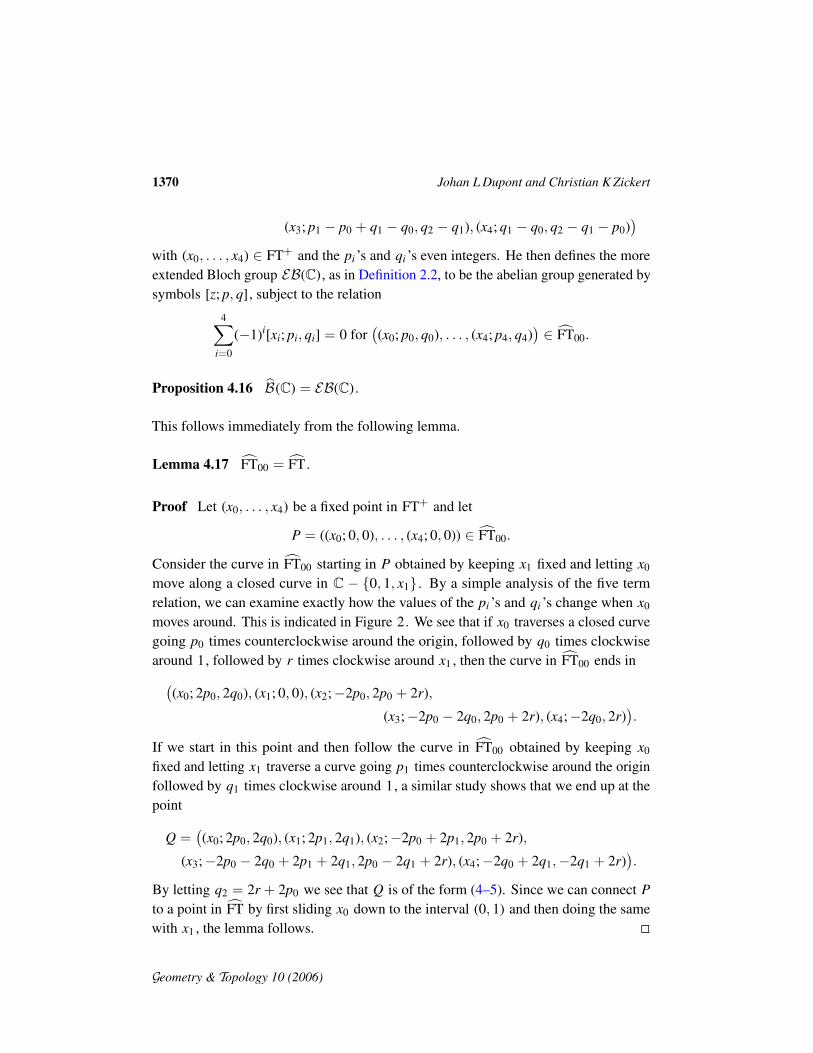
move along a closed curve in C − {0, 1, x1}. By a simple analysis of the five termrelation, we can examine exactly how the values of the pi ’s and qi ’s change when x0
moves around. This is indicated in Figure 2. We see that if x0 traverses a closed curvegoing p0 times counterclockwise around the origin, followed by q0 times clockwisearound 1, followed by r times clockwise around x1 , then the curve in FT00 ends in(
(x0; 2p0, 2q0), (x1; 0, 0), (x2;−2p0, 2p0 + 2r),
(x3;−2p0 − 2q0, 2p0 + 2r), (x4;−2q0, 2r)).
If we start in this point and then follow the curve in FT00 obtained by keeping x0
fixed and letting x1 traverse a curve going p1 times counterclockwise around the originfollowed by q1 times clockwise around 1, a similar study shows that we end up at thepoint
Q =((x0; 2p0, 2q0), (x1; 2p1, 2q1), (x2;−2p0 + 2p1, 2p0 + 2r),
(x3;−2p0 − 2q0 + 2p1 + 2q1, 2p0 − 2q1 + 2r), (x4;−2q0 + 2q1,−2q1 + 2r)).
By letting q2 = 2r + 2p0 we see that Q is of the form (4–5). Since we can connect Pto a point in FT by first sliding x0 down to the interval (0, 1) and then doing the samewith x1 , the lemma follows.
Geometry & Topology 10 (2006)
A dilogarithmic formula for the Cheeger–Chern–Simons class 1371
O
x1
1
x0
p0
p2
p3
p4
q0
q2
q4
q3
Figure 2: The lines in the figure are the cuts of the function sending z to (Log(z),Log( 11−z )) in
the xi –plane, i = 0, 2, 3, 4, when y = x1 is fixed. The relevant values of pi and qi increase by2 whenever x0 crosses the relevant line in the direction indicated by the arrows.
References
[1] J Cheeger, J Simons, Differential characters and geometric invariants, from: “Geome-try and topology (College Park, Md., 1983/84)”, Lecture Notes in Math. 1167, Springer,Berlin (1985) 50–80 MR827262
[2] S S Chern, J Simons, Characteristic forms and geometric invariants, Ann. of Math.(2) 99 (1974) 48–69 MR0353327
[3] J L Dupont, The dilogarithm as a characteristic class for flat bundles, J. Pure Appl.Algebra 44 (1987) 137–164 MR885101
[4] J L Dupont, Scissors congruences, group homology and characteristic classes, NankaiTracts in Mathematics 1, World Scientific Publishing Co., River Edge, NJ (2001)MR1832859
[5] J L Dupont, W Parry, C-H Sah, Homology of classical Lie groups made discreteII: H2,H3, and relations with scissors congruences, J. Algebra 113 (1988) 215–260MR928063
[6] J L Dupont, C H Sah, Scissors congruences II, J. Pure Appl. Algebra 25 (1982)159–195 MR662760
[7] W D Neumann, Extended Bloch group and the Cheeger–Chern–Simons class, Geom.Topol. 8 (2004) 413–474 MR2033484
[8] W D Neumann, J Yang, Bloch invariants of hyperbolic 3–manifolds, Duke Math. J. 96(1999) 29–59 MR1663915
Geometry & Topology 10 (2006)
1372 Johan L Dupont and Christian K Zickert
[9] W Parry, C-H Sah, Third homology of SL(2,R) made discrete, J. Pure Appl. Algebra30 (1983) 181–209 MR722372
[10] C-H Sah, Homology of classical Lie groups made discrete III, J. Pure Appl. Algebra 56(1989) 269–312 MR982639
Department of Mathematics, University of AarhusDK-8000 Èrhus, Denmark
Department of Mathematics, Columbia UniversityNew York, NY 10027, USA
[email protected], [email protected]
Proposed: Shigeyuki Morita Received: 2 August 2005Seconded: Joan Birman, Robion Kirby Revised: 2 August 2006
Geometry & Topology 10 (2006)