A dispersion and norm preserving finite difference scheme with transparentboundary conditions for the Dirac equation in (1+1)D

Rene Hammera,∗, Walter Potza, Anton Arnoldb

aInstitut fur Physik, Karl-Franzens-Universitat Graz, Universitatsplatz 5, 8010 Graz, AustriabInstitut fur Analysis und Scientific Computing, TU-Wien, Wiedner Hauptstr. 8, 1040 Wien, Austria

Abstract

A finite difference scheme is presented for the Dirac equation in (1+1)D. It can handle space- and time-dependent mass and potential terms and utilizes exact discrete transparent boundary conditions (DTBCs).Based on a space- and time-staggered leap-frog scheme it avoids fermion doubling and preserves the disper-sion relation of the continuum problem for mass zero (Weyl equation) exactly.Considering boundary regions, each with a constant mass and potential term, the associated DTBCs arederived by first applying this finite difference scheme and then using the Z-transform in the discrete timevariable. The resulting constant coefficient difference equation in space can be solved exactly on each of thetwo semi-infinite exterior domains. Admitting only solutions in l2 which vanish at infinity is equivalent toimposing outgoing boundary conditions. An inverse Z-transformation leads to exact DTBCs in form of aconvolution in discrete time which suppress spurious reflections at the boundaries and enforce stability ofthe whole space-time scheme.An exactly preserved functional for the norm of the Dirac spinor on the staggered grid is presented. Sim-ulations of Gaussian wave packets, leaving the computational domain without reflection, demonstrate thequality of the DTBCs numerically, as well as the importance of a faithful representation of the energy-momentum dispersion relation on a grid.

Keywords: Dirac equation, finite difference, leap-frog, fermion doubling

1. Introduction

We start out with a brief summary regarding important properties of the Dirac equation, its role playedin physics, existing numerical schemes for its solution, and the issue of open boundaries.

1.1. The Dirac equation

Next to its fundamental role in relativistic quantum mechanics and field theory, which provide the foun-dation of modern nuclear and high energy physics [1, 2], the Dirac equation has received a rapidly growingimportance in condensed matter systems as well. Especially, in the context of the recent experimental real-ization of graphene [3], 2D and 3D topological insulators [4, 5], and optical lattices [6–8] the Dirac equationdescribes the underlying physics as an effective field theory. Historically it was proposed by Dirac with hisingenious idea of linearizing the square root of the relativistic energy momentum relation by the introductionof Dirac matrices and multi-component wave functions, nowadays known as Dirac spinors. Imposing thecondition that the twofold application of this Dirac operator onto the spinor must yield the Klein-Gordonequation, leads to the Clifford algebra for the Dirac matrices. In (1+1)D and (2+1)D the minimum dimen-sion for a representation of this group is two, whereas in (3+1)D the Dirac spinor must have a minimum

∗Corresponding authorEmail addresses: rene.hammer@uni-graz.at (Rene Hammer), walter.poetz@uni-graz.at (Walter Potz),

anton.arnold@tuwien.ac.at (Anton Arnold)

Preprint submitted to Elsevier September 13, 2013

of four components. However, one can work with two components if one accepts higher–order derivativesin space and time [1, 2]. The latter has lead to the prediction of anti-matter and the concept of the filledFermi sea in many-particle physics. Alternatively, the Dirac equation emerges from an investigation of thetransformation properties of spinors under the Lorentz group [9]. In condensed matter physics Dirac-likeequations arise in context of low-energy two-band effective models, e.g. in k · p perturbation theory or thetight-binding approximations [5]. Indeed, the study of Dirac fermion realizations has developed into one ofthe most exciting current topics of condensed matter physics [5].

In this work we restrict ourselves to a study of the (1+1)D Dirac equation and present a numerically stablescheme for its solution under open boundary conditions. The latter are motivated by a particle transportsituation, as well as the fact that, unlike for the Schrodinger particle, a deep one-particle potential doesnot ensure confinement for Dirac particles. In its Schrodinger form, also called the standard or Pauli-Diracform, the (1+1)D Dirac equation may be written as (using c = 1, e = 1, and ~ = 1)

i∂tψ(x, t) = Hψ(x, t) , H = m(x, t)σz − i∂xσx − V (x, t)112 . (1)

The σi’s are the 2×2 Hermitian anti-commuting Pauli-matrices, and 112 is the identity matrix. x ∈ R, t ∈ R+,

and ψ =

(uv

)

∈ C2 is the complex 2-spinor. m,V ∈ R represent, respectively, a space- and time-dependent

mass and scalar potential. For constant coefficients, Fourier-transformation in the space and time variableand solving the eigenvalue problem gives the energy spectrum E± = ±

√

m2 + p2. In the physical groundstate all negative energy states are filled with fermions. Empty negative energy states are reinterpreted asfilled hole states (anti-particles) with positive energy, in analogy to multi-band systems in (non-relativistic)condensed matter physics [1]. The norm of the spinor is defined as |ψ(x, t)|2 =

√

|u(x, t)|2 + |v(x, t)|2, andits square can be interpreted as the probability density in space for given time t. The norm is conservedbecause Eq. eqrefdirac-eq is of Schrodinger form and H is Hermitian [1]. Global gauge-invariance holds asfor the case of the Schrodinger equation: the addition of a constant V simply adds a phase to the solution.The free Dirac equation has various other symmetries [1, 10]. First there are the continuous transformationsof spatial rotation (only meaningful for more than one space dimension) which, with the Lorentz boost, formthe Lorentz group. Together with space and time translations, they form the Poincare group. The latteris the fundamental group in particle physics, but is of minor importance in solid state physics because thecrystal lattice necessarily breaks these continuous symmetries. The discrete symmetries holding for arbitraryconstants m ∈ R, V ∈ R are space reflection (parity) and time reversal symmetry which will also be presentin the finite difference scheme.

1.2. Numerical aspects

Several schemes have been proposed and used for particle transport simulations based on the time-dependent Dirac equation. For a numerical treatment one has to discretize the continuum problem either inreal- or Fourier-space, or a combination thereof. Real-space schemes are, for example, the finite-difference[11–13] and finite-element methods [14], whereas the spectral methods [15] are examples for the momentumspace approach. Split-operator methods separate the time-evolution operator into several parts, with eachof them depending only on either momentum or position [16, 17]. There also exists a coordinate space split-operator method which transforms the Dirac equation into an advection equation and uses its characteristicsolutions [18]. While having the advantage of a natural implementation of space- and time dependentpotential and mass terms, the finite-difference and finite-element schemes have to deal with the issue offermion doubling, which means that, for a given sign of the energy, there are two (or more) extrema in them 6= 0 energy-momentum dispersion relation instead of the single one of the continuum problem [12]. In factthe ’Nielsen-Ninomiya no-go theorem’ forbids the existence of a single fermion flavor for chirally invariantfermions on a regular grid without breaking either translational invariance, locality, or Hermiticity [19]. In(1+1)D one can get rid of the fermion doubling using a staggered grid for the two spinor components. Thisis equivalent to taking the left-sided first-order derivative operator for one component of the spinor and theright-sided for the other one [12]. One obtains a monotonic dispersion relation with only one minimum.Here we present a scheme which provides an even better result by applying staggering to both the space

2

and the time coordinate. This yields a numerical scheme which preserves the exact dispersion relation ofthe continuum problem for the special choice of the ratio between time and space grid r := ∆t/∆x = 1and mass m = 0. For m,V 6= 0 and r = 1 the dispersion relation improves for all possible wave-numbersk ∈ [−π/∆x, π/∆x] with the refinement of the grid. For ∆x→ 0 the numerical dispersion relation becomesidentical to the continuum one. This is not true for most finite difference schemes in general and, to ourknowledge, no finite difference scheme with this property for the Dirac equation has been reported before.

Let us mention that numerical methods for the (1+1)D non-linear Dirac (NLD) equation also got someattention in the literature [20]. Besides being an interesting playground on its own, it might also have somephysical relevance by incorporating electron self-interaction into the Dirac equation. Scalar self-interactionleads to the Soler model [21], whereas vector-like inclusion of the self-interaction leads to the Thirring model[22]. Interestingly, the latter is S-dual to the quantum sine-Gordon model [22]. In contrast to the linearDirac equation it provides solitary wave solutions, standing wave solutions, and collapse after collision oftwo solitary waves [20]. As already for the Dirac equation, analytic solutions are rare, most of the behaviorof the NLD equation can only be investigated numerically [20]. For this purpose plenty of algorithms can befound in the literature. Without claim to completeness, they are of Crank-Nicholson type [23–25], explicitfinite difference schemes [20, 26], spectral schemes [27, 28], Runge-Kutta methods [29, 30], and moving meshmethods [31].

Remarkably, for the finite difference method no effort was made so far to eliminate the spurious solutions,e.g. by staggering the grid for the spinor components. Being well aware of the different behavior of the NLDequation, we think our scheme could also have some relevance there. At least it could serve to solve the linearpart in the operator-splitting method, thus avoiding the transformation to Fourier space. From a physicsperspective, however, the most natural way for the incorporation of self-consistency (e.g., self-interaction)is to solve the standard Dirac equation self-consistently and in parallel to the differential equations for theexternal potentials which appear in the former. A brief discussion will be given in the Conclusions in Sect.5.

1.3. Boundary conditions

For a numerical treatment of a differential equation, such as the Dirac equation, the number of degrees offreedom must be finite. In addition to the discretization of the time and space variable in a real-space schemeone has to restrict the simulation domain to a finite region in time and space. Then, appropriate boundaryconditions are needed to ensure that the solution obtained within the finite domain is (at least) a goodapproximation to the solution of the whole space problem. Generally, the time-dependent Dirac equation issolved as an initial-value problem in time. The standard approach for the derivation of spatial transparentboundary conditions (TBCs), e.g. for the Schrodinger equation, has been to solve the continuous exteriorproblem by using the Laplace-transformation in time and to discretize the continuous TBCs afterwards [32].To avoid stability problems [33] and spurious reflections at the boundary from inconsistent discretizationschemes, recently, a new improved approach in which the whole domain is discretized first and then solvedexactly in the constant-coefficient exterior domains using a Z-transform in time has been developed for theSchrodinger equation [34, 37]. In this way one maintains the stability properties of the scheme on the wholespace and avoids inconsistent discretization for the simulation region and the boundary conditions. Theresulting discrete transparent boundary conditions (DTBCs) which are non-local in time are exact in thesense that they do not introduce a procedural error. An alternative approach which, in most cases is easierto handle because an inverse Z-transform can be avoided, is to discretize in space only, derive TBCs, anddiscretize in time thereafter. This has been done with good results for hyperbolic systems [38–40]. Howeverfor the proposed scheme, where the good properties regarding dispersion and conservation of norm arisefrom the simultaneous discretization of space and time in an interlaced manner, paying the extra price inform of an inverse Z-transformation is well justified. Therefore we follow the fully discrete approach of [34]to develop TBCs for the time- and space-staggered leap-frog scheme. Furthermore, in order to preserve thecovariant symmetry of the Dirac equation on a space-time grid, time and space coordinates must be treatedon an equal footing. This is particularly important in higher dimensions.

As a major difference to the Schrodinger equation one should mention that a massless relativistic particlecannot be trapped by a scalar one-particle potential [1]. The same holds for massive relativistic particles

3

with energy E, when the potential depth V is such that E + mc2 > V > E − mc2. This phenomenonis related to the Klein paradox and is due to the two-band-nature of the dispersion relation, consistingof an electron and a positron band. One is necessarily dealing with a scattering problem whenever thereare no bound states supported by the Hamiltonian. Then, for initial data which are compactly supportedon the computational domain, the solution always reaches the boundary after a finite time. For simulationtimes beyond that threshold, open boundary conditions are required to close the finite difference scheme in aparticle transport situation, similar to non-relativistic particle transport simulations in nano devices [35, 36].

2. Continuous transparent boundary conditions for the Dirac equation in (1+1)D

In this section we derive continuous TBCs for the Dirac equation Eq. (1). We divide the entire spaceinto the computational domain (0, L), and the semi-infinite exterior domains (−∞, 0] and [L,∞). The massis assumed to be constant m(x, t) = m and the potential is constant in space V (x, t) = V (t) in the exteriordomains. This reduces to the case V = 0 with the following gauge change of the spinor:

ψ(x, t) = eiV(t)χ(x, t) with V(t) =∫ t

0

V (s)ds . (2)

With χ = (u, v), in the exterior, we have

i

(u(x, t)v(x, t)

)

t

=

(m −i∂x−i∂x −m

)(u(x, t)v(x, t)

)

. (3)

The multiplication with σx and a Laplace transformation with respect to the time variable leads to

(u(x, s)v(x, s)

)

x

=

(0 −s+ im

−s− im 0

)(u(x, s)v(x, s)

)

. (4)

Eq. (4) has the general solution

(u(x, s)v(x, s)

)

= c1

(−s+ im

− +√s2 +m2

)

e−+√s2+m2x + c2

(−s+ im+√s2 +m2

)

e+√s2+m2x , (5)

where +√

is written for the square root with positive real part. Because the solution must be in L2(R)the constant c2 must vanish on the right exterior domain. For the same reason c1 must be zero on the leftexterior domain. Therefore, the boundary conditions on the right boundary are

∂xu(x, s)∣∣x=L

= − +√

s2 +m2 u(L, s) and ∂xv(x, s)∣∣x=L

= − +√

s2 +m2 v(L, s) . (6)

On the left boundary one gets

∂xu(x, s)∣∣x=0

=+√

s2 +m2 u(0, s) and ∂xv(x, s)∣∣x=0

=+√

s2 +m2 v(0, s) . (7)

The structure for both spinor components and both boundaries is the same, so we proceed with u on theright boundary. First we derive boundary conditions as a Neumann-to-Dirichlet map by writing

u(L, s) = − 1+√s2 +m2

∂xu(x, s)∣∣x=L

. (8)

Then the inverse Laplace transformation leads to the convolution at the right boundary:

u(L, t) = −J0(mt) ∗t ∂xu(x, t)∣∣x=L

= −∫ t

0

J0(mτ)∂xu(L, t− τ) dτ , (9)

4

with J0 being the Bessel function of first kind. Analogously for the left boundary:

u(0, t) = J0(mt) ∗t ∂xu(x, t)∣∣x=0

. (10)

Finally, this leads with the gauge Eq. (2) for V 6= 0 to the TBCs in the form of a Neumann-to-Dirichletmap:

ψ(L, t) = −eiVr(t){

J0(mt) ∗t[

∂xψ(x, t)∣∣x=L

e−iVr(t)]}

. . . right TBC , (11)

ψ(0, t) = eiVl(t){

J0(mt) ∗t[

∂xψ(x, t)∣∣x=0

e−iVr(t)]}

. . . left TBC . (12)

For the derivation of TBCs in the form of a Dirichlet-to-Neumann map we write:

∂xu(x, s)∣∣x=L

= −g(s)u(L, s) , (13)

with:

g(s) :=+√

s2 +m2 =

(

s2 +m2

+√s2 +m2

− s

)

+ s . (14)

We use

f(s) :=1

+√s2 +m2

L−1

→ f(t) = J0(mt) (15)

and

s2f(s)− sf(0)L−1

→ m2J ′′0 (mt) . (16)

This leads to the following inverse Laplace transform of g(s):

g(s)L−1

→ g(t) = m2[J ′′0 (mt) + J0(mt)

]+ δ′ =

m2

2

[J2(mt) + J0(mt)

]+ δ′ , (17)

where δ′ is the first derivative of the delta distribution. Then the TBC as a Dirichlet-to-Neumann map onthe right boundary is

∂xψ(x, t)∣∣x=L

= −eiVr(t){m2

2

[J2(mt) + J0(mt)

]∗t ψ(L, t)e−iVr(t) + ∂tψ(L, t)e

−iVr(t)}

. (18)

On the left boundary one gets

∂xψ(x, t)∣∣x=0

= eiVr(t){m2

2

[J2(mt) + J0(mt)

]∗t ψ(0, t)e−iVr(t) + ∂tψ(0, t)e

−iVr(t)}

. (19)

Discretizations of Eqs. (11) and (12) or Eqs. (18) and (19) can serve as boundary conditions for arbitraryfinite difference discretizations of the Dirac equation Eq. (1). But one has to be aware of the fact thatinconsistent discretization of the differential equation and the associated boundary conditions usually leadsto spurious reflections or even instability. As already mentioned in the introduction we will therefore firstapply the discretization scheme to Eq. (1) for the the boundary regions also and derive the associated TBCsby Z-transformation. Eqs. (11), (12), (18), and (19) serve as a guide to gain intuition for the behavior ofthe convolution coefficients.

5

3. Time- and space-staggered leap-frog scheme

Leap-frog time-stepping, in combination with a staggered spatial grid, plays a special role among thefinite difference methods because, in addition to the elimination of the fermion-doubling problem, it provesto be dispersion relation preserving in (1+1)D for the ‘golden ratio’ of r = ∆t/∆x = 1, m = 0, and V = 0(Weyl equation). Moreover, for m 6= 0 and/or V 6= 0 the dispersion relation is still monotone and improveswith a refinement of the grid. It is identical to the exact analytic dispersion when ∆t,∆x → 0, for fixedr = 1. This is particularly important for simulations where the whole possible range of the wave numbersk ∈

[− π

∆x ,π∆x

]is used, for example, in strong external fields. An initial wave-packet which consists only

of wave-components near k = 0 may acquire high wave number components due to strong spatial and/ortemporal changes of potential and/or mass.

For schemes with non-monotonic dispersion a problem can also arise at the boundary. The modes of sucha scheme consist of additional, spurious, numerically generated modes on the lattice which, nevertheless,must be accounted for in the DTBCs for consistency. This requires special attention at the boundary becauseimproper realization of the boundary condition may lead to ‘energy’ transfer between the modes, spuriousreflections, and eventually instability (see e.g. [40]). A correct dispersion relation means correct phase andgroup velocity on the grid and is essential for faithful long-time propagation studies. We now present sucha scheme.

3.1. The discretization scheme

We shall consider the following leap-frog discretization of the Dirac equation in Pauli-Dirac form givenin Eq.(1):

un+1/2j − u

n−1/2j

∆t+ i(mn

j − V nj )un+1/2j + u

n−1/2j

2+

(Dvn)j∆x

= 0 , (20)

vn+1j−1/2 − vnj−1/2

∆t− i(m

n+1/2j−1/2 + V

n+1/2j−1/2 )

vn+1j−1/2 + vnj−1/2

2+

(Dun+1/2)j−1/2

∆x= 0 , (21)

with j ∈ Z, n ∈ N. Here we used the notation ψ(x, t) =[u(x, t), v(x, t)

]with u(xj , t

n−1/2) ≈ un−1/2j and

v(xj−1/2, tn) ≈ vnj−1/2. The symmetric spatial difference operator is defined as (Dvn)j = vnj+1/2 − vnj−1/2

and (Dun+1/2)j−1/2 = un+1/2j − u

n+1/2j−1 . For the mass and potential term we use the averages gnj =

(gn+1/2j + g

n−1/2j

)/2 for the integer spacial grid-points and g

n+1/2j−1/2 =

(

gn+1j−1/2 + gnj−1/2

)

/2 for the half-

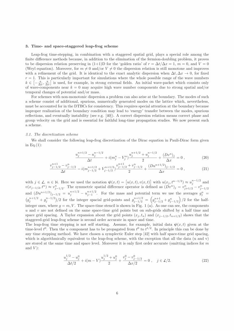
integer ones, where g = m,V . The space-time stencil is shown in Fig. 1 (a). As one can see, the componentsu and v are not defined on the same space-time grid points but on sub-grids shifted by a half time andspace grid spacing. A Taylor expansion about the grid points (xj , tn) and (xj−1/2, tn+1/2) shows that thestaggered-grid leap-frog scheme is second order accurate in space and time.The leap-frog time stepping is not self starting. Assume, for example, initial data ψ(x, t) given at thetime-level t0. Then the u component has to be propagated from t0 to t1/2. In principle this can be done byany time stepping method. We have chosen a symplectic Euler step [42] with half space-time grid spacing,which is algorithmically equivalent to the leap-frog scheme, with the exception that all the data (u and v)are stored at the same time and space level. Moreover it is only first order accurate (omitting indices for mand V ):

u1/2j − u0j∆t/2

+ i(m− V )u1/2j + u0j

2+v0j − v0j−1/2

∆x/2= 0 , j ∈ Z/2. (22)

6

Figure 1: (color online). (a) Staggered-grid scheme for Dirac equation in Pauli-Dirac form with leap-frog time-stepping; (b)the algorithmically equivalent (except for starting procedure) symplectic Euler time-stepping.

After this first initialization step the u-component is stored only at integer and the v-component at halfinteger spatial points. With a relabeling of the indices, the algorithm Eq. (21) can be written as follows:

un+1j − unj

∆t+ i(m− V )

un+1j + unj

2+vnj − vnj−1

∆x= 0 ,

vn+1j − vnj

∆t− i(m+ V )

vn+1j + vnj

2+un+1j+1 − un+1

j

∆x= 0 , (23)

with j ∈ Z, n ∈ N0. Here we use the approximations unj ≈ u(xj−1/4, tn−1/4), vnj ≈ v(xj+1/4, t

n+1/4) (seeFig. 1 (b)). Rearranging of terms leads to the following equations for the explicit recursive update

un+1j =

2− i(m− V )∆t

2 + i(m− V )∆tunj − 2∆t/∆x

2 + i(m− V )∆t

(

vnj − vnj−1

)

, (24)

vn+1j =

2 + i(m+ V )∆t

2− i(m+ V )∆tvnj − 2∆t/∆x

2− i(m+ V )∆t

(

un+1j+1 − un+1

j

)

. (25)

The starting procedure for the leap-frog scheme with a symplectic Euler step of half grid-size is especiallysuitable since symplectic Euler is algorithmically equivalent to the leap-frog staggered-grid scheme and hasthe same dispersion relation for equal ratio r.

3.2. Von Neumann stability analysis

For constant coefficients in Eq. (23), Fourier analysis can be used to perform a von Neumann stabilityanalysis and to derive the dispersion relation for the whole space problem. A Fourier transform in space ofEq. (23) leads to

(1∆t +

i(m−V )2 0

e−ik∆x−1∆x

1∆t −

i(m+V )2

)

︸ ︷︷ ︸

=:A

(un+1

vn+1

)

+

(

− 1∆t +

i(m−V )2

1−eik∆x

∆x

0 − 1∆t −

i(m+V )2

)

︸ ︷︷ ︸

=:B=−A∗

(un

vn

)

= 0 . (26)

Using the definitions ξ = k∆x, µ = m∆t, ν = V∆t, and r = ∆t/∆x the eigenvalues of the amplificationmatrix

G = −A−1B = A−1A∗ =

(2i−ν+µ2i+ν−µ

2ir(eiξ−1)2i+ν−µ

2r(1−e−iξ)(2+iν−iµ)4−ν2−4νi+µ2

4+ν2−µ2+4µi+8r2[cos ξ−1]4−ν2−4νi+µ2

)

(27)

are computed by means of

λ± = P/2±√(P/2

)2 −Q , (28)

7

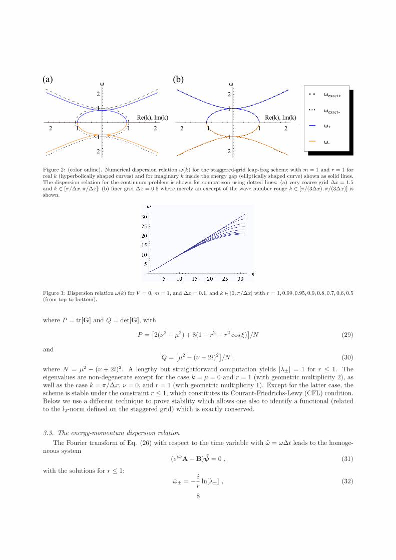
Figure 2: (color online). Numerical dispersion relation ω(k) for the staggered-grid leap-frog scheme with m = 1 and r = 1 forreal k (hyperbolically shaped curves) and for imaginary k inside the energy gap (elliptically shaped curve) shown as solid lines.The dispersion relation for the continuum problem is shown for comparison using dotted lines: (a) very coarse grid ∆x = 1.5and k ∈ [π/∆x, π/∆x]; (b) finer grid ∆x = 0.5 where merely an excerpt of the wave number range k ∈ [π/(3∆x), π/(3∆x)] isshown.

Figure 3: Dispersion relation ω(k) for V = 0, m = 1, and ∆x = 0.1, and k ∈ [0, π/∆x] with r = 1, 0.99, 0.95, 0.9, 0.8, 0.7, 0.6, 0.5(from top to bottom).

where P = tr[G] and Q = det[G], with

P =[2(ν2 − µ2) + 8(1− r2 + r2 cos ξ)

]/N (29)

andQ =

[µ2 − (ν − 2i)2

]/N , (30)

where N = µ2 − (ν + 2i)2. A lengthy but straightforward computation yields |λ±| = 1 for r ≤ 1. Theeigenvalues are non-degenerate except for the case k = µ = 0 and r = 1 (with geometric multiplicity 2), aswell as the case k = π/∆x, ν = 0, and r = 1 (with geometric multiplicity 1). Except for the latter case, thescheme is stable under the constraint r ≤ 1, which constitutes its Courant-Friedrichs-Lewy (CFL) condition.Below we use a different technique to prove stability which allows one also to identify a functional (relatedto the l2-norm defined on the staggered grid) which is exactly conserved.

3.3. The energy-momentum dispersion relation

The Fourier transform of Eq. (26) with respect to the time variable with ω = ω∆t leads to the homoge-neous system

(eiωA+B)ψ = 0 , (31)

with the solutions for r ≤ 1:

ω± = − i

rln[λ±] , (32)

8

where λ± is given in Eq. (28). By setting µ, ν = 0 they reduce to

ω± = − i

rln

{

1 + r2(cos ξ − 1

)±√[

r2(cos ξ − 1

)+ 1]2

− 1

}

, (33)

and with the choice r = 1 they read

ω± = −i ln(

cos ξ ±√

cos2 ξ − 1)

= −i ln(

cos ξ ± i sin ξ)

= ±ξ . (34)

Thus for µ, ν = 0, and r = 1 the linear dispersion of the continuum problem (Weyl equation) is exactlypreserved.

The connection to the phase of the growth factor (i.e. eigenvalues of G) can be established via

ω± = − i

rln[λ±] = − i

r[ln |λ±|+ i arg(λ±) + 2πin] =

1

r[arg(λ±) + 2πn] . (35)

In Fig. 2 the dispersion relation for a rather coarse grid with ∆x = 1.5 is compared to that of a finer oneusing ∆x = 0.5, for m = 1, V = 0, and r = 1. Clearly, the quality of the numerical dispersion relationimproves for a finer grid and, for all wave-numbers k ∈ [−π/∆x, π/∆x], it approaches the continuum formin the limit ∆x → 0 and r = 1. In Fig. 3 the dispersion relation for fixed values of m and V is shown forseveral values of r and ∆x = 0.1.

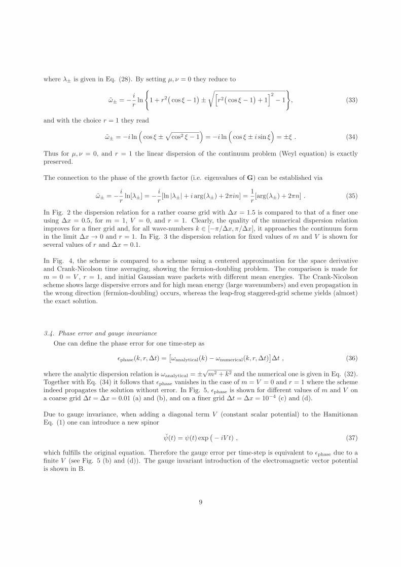
In Fig. 4, the scheme is compared to a scheme using a centered approximation for the space derivativeand Crank-Nicolson time averaging, showing the fermion-doubling problem. The comparison is made form = 0 = V , r = 1, and initial Gaussian wave packets with different mean energies. The Crank-Nicolsonscheme shows large dispersive errors and for high mean energy (large wavenumbers) and even propagation inthe wrong direction (fermion-doubling) occurs, whereas the leap-frog staggered-grid scheme yields (almost)the exact solution.

3.4. Phase error and gauge invariance

One can define the phase error for one time-step as

ǫphase(k, r,∆t) =[ωanalytical(k)− ωnumerical(k, r,∆t)

]∆t , (36)

where the analytic dispersion relation is ωanalytical = ±√m2 + k2 and the numerical one is given in Eq. (32).

Together with Eq. (34) it follows that ǫphase vanishes in the case of m = V = 0 and r = 1 where the schemeindeed propagates the solution without error. In Fig. 5, ǫphase is shown for different values of m and V ona coarse grid ∆t = ∆x = 0.01 (a) and (b), and on a finer grid ∆t = ∆x = 10−4 (c) and (d).

Due to gauge invariance, when adding a diagonal term V (constant scalar potential) to the HamitionanEq. (1) one can introduce a new spinor

ψ(t) = ψ(t) exp(− iV t) , (37)

which fulfills the original equation. Therefore the gauge error per time-step is equivalent to ǫphase due to afinite V (see Fig. 5 (b) and (d)). The gauge invariant introduction of the electromagnetic vector potentialis shown in B.

9

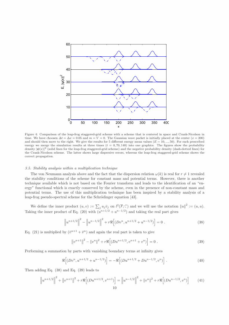
Figure 4: Comparison of the leap-frog staggered-grid scheme with a scheme that is centered in space and Crank-Nicolson intime. We have choosen ∆t = ∆x = 0.05 and m = V = 0. The Gaussian wave packet is initially placed at the center (x = 200)and should then move to the right. We give the results for 5 different energy mean values (E = 10, ..., 50). For each prescribedenergy we merge the simulation results at three times (t = 0, 70, 140) into one graphics. The figures show the probabilitydensity |ψ(x)|2 (solid lines for the leap-frog staggered-grid scheme) and the negative probability density (dash-dotted lines) forthe Crank-Nicolson scheme. The latter shows large dispersive errors, whereas the leap-frog staggered-grid scheme shows thecorrect propagation.

3.5. Stability analysis within a multiplication technique

The von Neumann analysis above and the fact that the dispersion relation ω(k) is real for r 6= 1 revealedthe stability conditions of the scheme for constant mass and potential terms. However, there is anothertechnique available which is not based on the Fourier transform and leads to the identification of an “en-ergy” functional which is exactly conserved by the scheme, even in the presence of non-constant mass andpotential terms. The use of this multiplication technique has been inspired by a stability analysis of aleap-frog pseudo-spectral scheme for the Schrodinger equation [43].

We define the inner product (u, v) :=∑

j uj vj on l2(Z;C) and we will use the notation ‖u‖2 := (u, u).

Taking the inner product of Eq. (20) with (un+1/2 + un−1/2) and taking the real part gives

∥∥∥un+1/2

∥∥∥

2

−∥∥∥un−1/2

∥∥∥

2

+ rℜ[

(Dvn, un+1/2 + un−1/2)]

= 0 . (38)

Eq. (21) is multiplied by (vn+1 + vn) and again the real part is taken to give

∥∥vn+1

∥∥2 − ‖vn‖2 + rℜ

[

(Dun+1/2, vn+1 + vn)]

= 0 . (39)

Performing a summation by parts with vanishing boundary terms at infinity gives

ℜ[

(Dvn, un+1/2 + un−1/2)]

= −ℜ[

(Dun+1/2 +Dun−1/2, vn)]

. (40)

Then adding Eq. (38) and Eq. (39) leads to

∥∥∥un+1/2

∥∥∥

2

+∥∥vn+1

∥∥2+ rℜ

[

(Dun+1/2, vn+1)]

=∥∥∥un−1/2

∥∥∥

2

+ ‖vn‖2 + rℜ[

(Dun−1/2, vn)]

(41)

10

Figure 5: The dependence of the phase error ǫphase on the wave vector k ∈ [0, π/∆x] for V = 0, m = 1, 2, 3, 4, 5 (from bottom

to top): (a) coarse grid ∆t = ∆x = 0.01, (c) fine grid ∆t = ∆x = 10−4; for V = 1, 2, 3, 4, 5 (from bottom to top), m = 0: (b)coarse grid ∆t = ∆x = 0.01, (d) fine grid ∆t = ∆x = 10−4. In (d) the functions exceed the plot-range, where the maxima forV = (1, 2, 3, 4, 5) are ǫphase = (1, 2, 3, 4, 5) ∗ 10−4 at k = 104π.

and one immediately identifies the conserved functional

Enr :=

∥∥∥un+1/2

∥∥∥

2

+∥∥vn+1

∥∥2+ rℜ

[

(Dun+1/2, vn+1)]

= const = E0r . (42)

With this result one obtains the stability condition for the scheme by using

∣∣∣ℜ[

(Dun+1/2, vn+1)]∣∣∣ ≤

∥∥∥un+1/2

∥∥∥

2

+∥∥vn+1

∥∥2. (43)

This gives the estimate∥∥∥un+1/2

∥∥∥

2

+∥∥vn+1

∥∥2 ≤ E0

r

1− r∀ n , (44)

for r < 1. The case r = 1 must be treated separately and one rewrites En1 as

En1 =

∑

j

|un+1/2j |2 + |vn+1

j+1/2|2 + ℜ

∑

j

(un+1/2j+1 − u

n+1/2j

)vn+1j+1/2 (45)

=1

2

∑

j

|un+1/2j − vn+1

j+1/2|2 +

1

2

∑

j

|un+1/2j+1 + vn+1

j+1/2|2 . (46)

11

Alternatively, when shifting indices, one obtains

En1 =

1

2

∑

j

|un+1/2j + vn+1

j−1/2|2 +

1

2

∑

j

|un+1/2j − vn+1

j+1/2|2 . (47)

Using 14 ‖a1 + a2‖2 ≤ 1

4

(‖a1 + b‖+ ‖a2 − b‖

)2 ≤ 12 ‖a1 + b‖2 + 1

2 ‖a2 − b‖2 gives

from Eq. (46):∥∥∥un+1/2

∥∥∥

2

:=∑

j

∣∣∣∣∣

un+1/2j + u

n+1/2j+1

2

∣∣∣∣∣

2

≤ En1 = E0

1 ∀n (48)

from Eq. (47):∥∥vn+1

∥∥2:=∑

j

∣∣∣∣∣

vn+1j−1/2 + vn+1

j+1/2

2

∣∣∣∣∣

2

≤ En1 = E0

1 ∀n

⇒∥∥∥un+1/2

∥∥∥

2

+∥∥vn+1

∥∥2 ≤ 2E0

1 . (49)

One easily verifies that ‖u‖ is a norm on l2(Z). Indeed, u = 0 implies uj = (−1)jλ for some λ ∈ C. Andu ∈ l2 then yields u = 0.

This allows us to conclude that the scheme is stable for all r = ∆t/∆x ≤ 1. Moreover we have identifiedthe functional which is conserved by the scheme (see Eq. (42)). In fact, it is conserved for arbitrary timeand space dependent m,V ∈ R.

3.6. Time-reversal invariance

The time reversal invariance of the scheme can easily be seen in Eqs. (20) and (21). One has to set∆t → −∆t and replace the role of the old and new time-levels n − 1/2 ↔ n + 1/2 and n ↔ n + 1. Thenone observes that the scheme for the backward propagation has exactly the same form as for the forwardpropagation and concludes the scheme is time-reversal invariant.

4. Discrete transparent boundary conditions for the staggered-grid leap-frog scheme

Having discussed the properties of the leap-frog scheme we now turn to the derivation of the associatedTBCs. Again, we divide the entire space into the computational domain (0, L), a left semi-infinite exteriordomain (−∞, 0], and a right semi-infinite exterior domain [L,∞). This corresponds to a typical devicesimulation geometry (scattering scenario) in which the nano-device is placed in the computational domainand the (macroscopic) contacts are represented by the exterior domains. We make the following simplifyingassumptions:

• The initial data ψ0(x) = ψ(0, x) is compactly supported inside the computational domain.

• In each exterior domain the mass m(x, t) = m and potential V (x, t) = V are constant in t and x.

Both assumption are made for simplicity but can be loosened when needed, as will be discussed below.

We first Z-transform Eq. (23) in t-direction on each of the exterior domains, j ∈ {. . . ,−2,−1, 0} andj ∈ {J, J +1, J +2, . . .}, and solve the resulting finite difference equations explicitly. Using the definition of

the Z-transform b(z) := Z(bn) =∞∑

n=0bnz

−n, its shifting property Z(bn+1) =∞∑

n=0bn+1z

−n =∞∑

n=1bnz

−n+1 =

12

zb(z)− zb0, and setting b0 = 0 (since the initial spinor is compactly supported on (0, L) ) we obtain

(1∆t (z − 1) + i(m−V )

2 (z + 1) 1∆x

z∆x 0

)(uj(z)vj(z)

)

(50)

+

(0 − 1

∆x

− z∆x

1∆t (z − 1)− i(m+V )

2 (z + 1)

)(uj−1(z)vj−1(z)

)

= 0 .

Translation from grid point j to j + 1 therefore is given by

(ujvj

)

=

(

1 ∆x∆t

1−zz + i(m+V )∆x

21+zz

∆x∆t (1− z)− i(m−V )∆x

2 (1 + z) 1 + ∆x2

z

[(1−z)2

∆t2 + iV 1−z2

∆t + (m2−V 2)(z+1)2

4

]

)(uj−1

vj−1

)

.

(51)

This can also be written as

(uj − uj−1

vj − vj−1

)

=

(

0 ∆x∆t

1−zz + i(m+V )∆x

21+zz

∆x∆t (1− z)− i(m−V )∆x

2 (1 + z) ∆x2

z

[(1−z)2

∆t2 + iV 1−z2

∆t + (m2−V 2)(z+1)2

4

]

)

︸ ︷︷ ︸

=:M

(uj−1

vj−1

)

,

(52)

where M :=

(0 ab c

)

fulfills ab = c. Solving the system Eq. (52) leads to

uj+1 − (2 + c)uj + uj−1 = 0 , (53)

whose characteristic equation has the roots:

τ1,2 = 1 +c

2±√

c+c2

4. (54)

The same result is obtained for the component v. Since τ1τ2 = 1, there is one decaying mode (as j → ∞)with |τ1| ≤ 1 and one increasing mode with |τ2| ≥ 1. In order to have a solution in l2(Z) one has to choosethe mode with |τ1| ≤ 1. At each boundary only one spinor component couples to the contact region. Thespinor components u and v, respectively, only need a right and a left TBC (see Eq. (23) and Fig. 1)

v0(z) = τ1(z)v1(z) (55)

uJ(z) = τ1(z)uJ−1(z)

Then, the inverse Z-transformed boundary conditions are in the form of a convolution in the discrete timevariable:

vn0 =n∑

k=0

τ(n−k)1 vk1 . (56)

unJ =n∑

k=0

τ(n−k)1 ukJ−1 . (57)

τ1(z) is a non-rational function of z, hence there is no easy way of finding an analytic expression for itsinverse Z-transformed in general. However, the poles and branch-points in the z-plane, which determine thegeneral behavior of their inverse Z-transformed in (discrete) real time n, can be identified. We give a brief

13

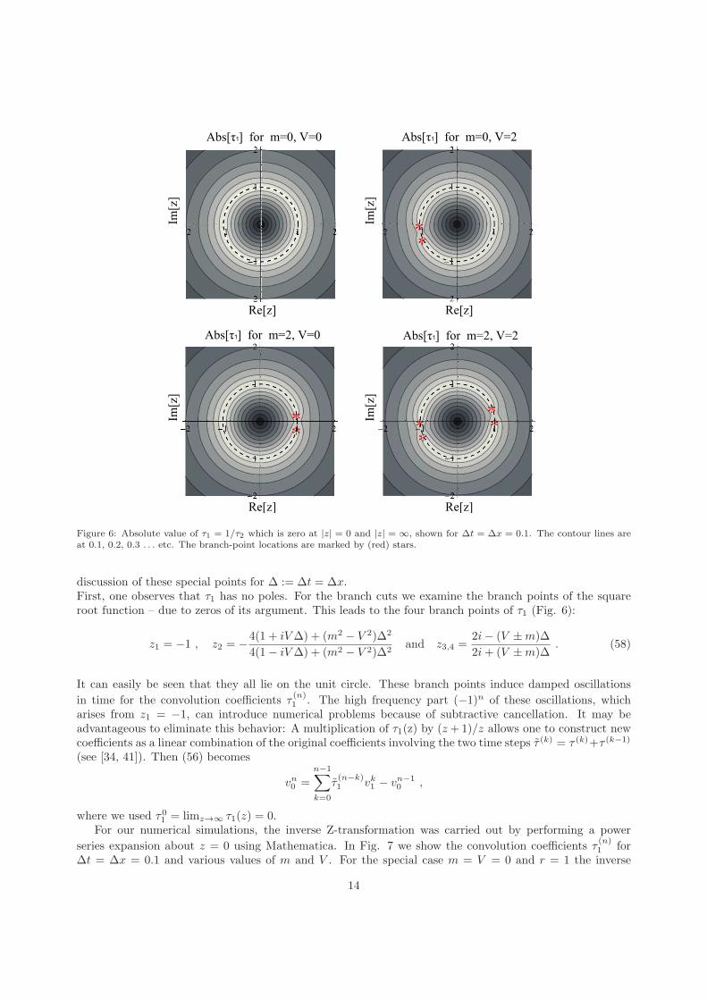
Figure 6: Absolute value of τ1 = 1/τ2 which is zero at |z| = 0 and |z| = ∞, shown for ∆t = ∆x = 0.1. The contour lines areat 0.1, 0.2, 0.3 . . . etc. The branch-point locations are marked by (red) stars.

discussion of these special points for ∆ := ∆t = ∆x.First, one observes that τ1 has no poles. For the branch cuts we examine the branch points of the squareroot function – due to zeros of its argument. This leads to the four branch points of τ1 (Fig. 6):

z1 = −1 , z2 = −4(1 + iV∆) + (m2 − V 2)∆2

4(1− iV∆) + (m2 − V 2)∆2and z3,4 =

2i− (V ±m)∆

2i+ (V ±m)∆. (58)

It can easily be seen that they all lie on the unit circle. These branch points induce damped oscillations

in time for the convolution coefficients τ(n)1 . The high frequency part (−1)n of these oscillations, which

arises from z1 = −1, can introduce numerical problems because of subtractive cancellation. It may beadvantageous to eliminate this behavior: A multiplication of τ1(z) by (z+1)/z allows one to construct newcoefficients as a linear combination of the original coefficients involving the two time steps τ (k) = τ (k)+τ (k−1)

(see [34, 41]). Then (56) becomes

vn0 =

n−1∑

k=0

τ(n−k)1 vk1 − vn−1

0 ,

where we used τ01 = limz→∞ τ1(z) = 0.For our numerical simulations, the inverse Z-transformation was carried out by performing a power

series expansion about z = 0 using Mathematica. In Fig. 7 we show the convolution coefficients τ(n)1 for

∆t = ∆x = 0.1 and various values of m and V . For the special case m = V = 0 and r = 1 the inverse

14

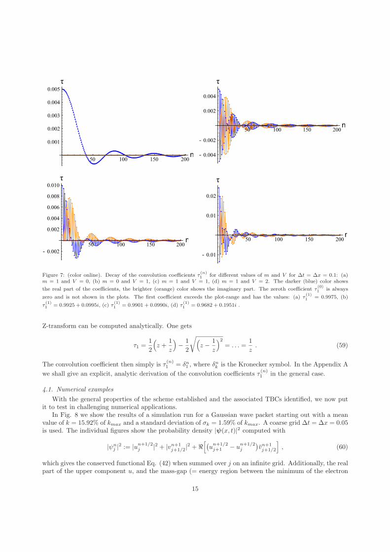
Figure 7: (color online). Decay of the convolution coefficients τ(n)1 for different values of m and V for ∆t = ∆x = 0.1: (a)

m = 1 and V = 0, (b) m = 0 and V = 1, (c) m = 1 and V = 1, (d) m = 1 and V = 2. The darker (blue) color shows

the real part of the coefficients, the brighter (orange) color shows the imaginary part. The zeroth coefficient τ(0)1 is always

zero and is not shown in the plots. The first coefficient exceeds the plot-range and has the values: (a) τ(1)1 = 0.9975, (b)

τ(1)1 = 0.9925 + 0.0995i, (c) τ

(1)1 = 0.9901 + 0.0990i, (d) τ

(1)1 = 0.9682 + 0.1951i .

Z-transform can be computed analytically. One gets

τ1 =1

2

(

z +1

z

)

− 1

2

√(

z − 1

z

)2

= . . . =1

z. (59)

The convolution coefficient then simply is τ(n)1 = δn1 , where δ

nk is the Kronecker symbol. In the Appendix A

we shall give an explicit, analytic derivation of the convolution coefficients τ(n)1 in the general case.

4.1. Numerical examples

With the general properties of the scheme established and the associated TBCs identified, we now putit to test in challenging numerical applications.

In Fig. 8 we show the results of a simulation run for a Gaussian wave packet starting out with a meanvalue of k = 15.92% of kmax and a standard deviation of σk = 1.59% of kmax. A coarse grid ∆t = ∆x = 0.05is used. The individual figures show the probability density |ψ(x, t)|2 computed with

|ψnj |2 := |un+1/2

j |2 + |vn+1j+1/2|

2 + ℜ[(un+1/2j+1 − u

n+1/2j

)vn+1j+1/2

]

, (60)

which gives the conserved functional Eq. (42) when summed over j on an infinite grid. Additionally, the realpart of the upper component u, and the mass-gap (= energy region between the minimum of the electron

15

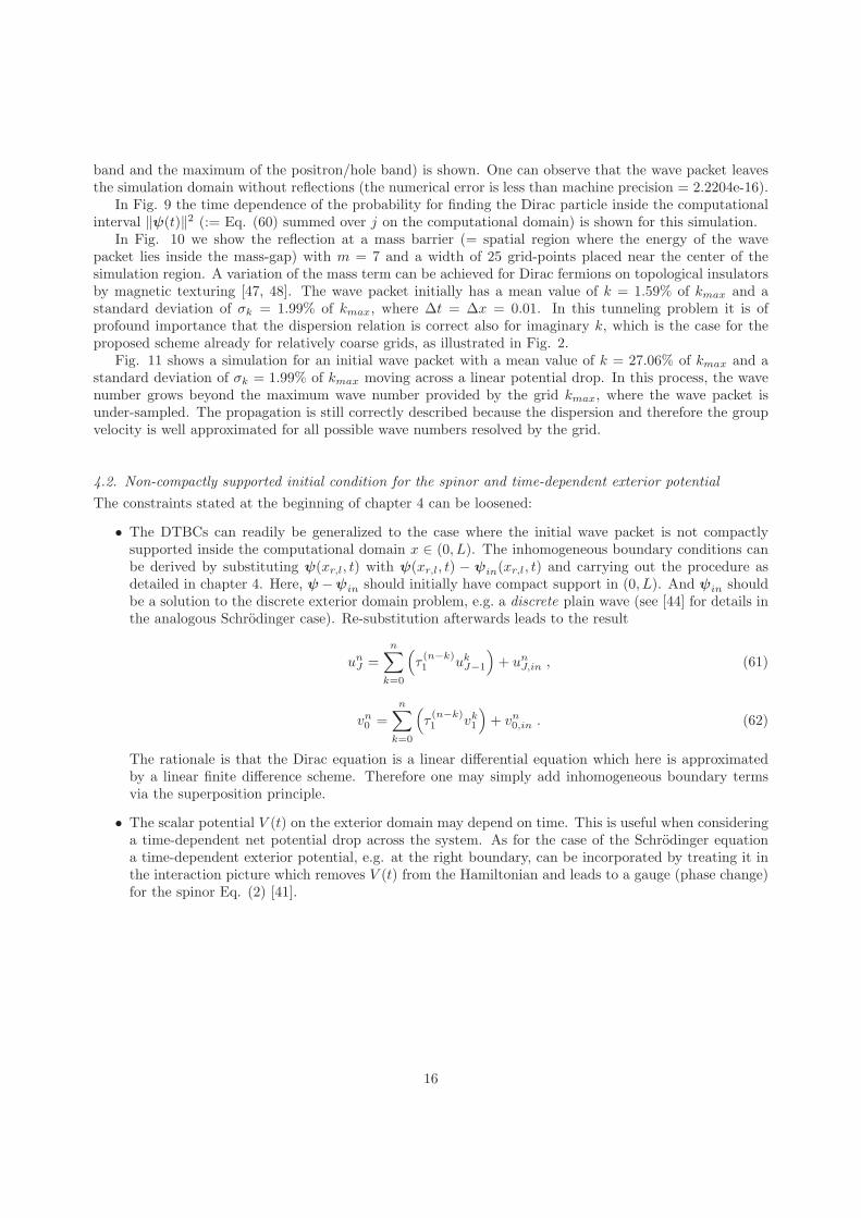
band and the maximum of the positron/hole band) is shown. One can observe that the wave packet leavesthe simulation domain without reflections (the numerical error is less than machine precision = 2.2204e-16).

In Fig. 9 the time dependence of the probability for finding the Dirac particle inside the computationalinterval ‖ψ(t)‖2 (:= Eq. (60) summed over j on the computational domain) is shown for this simulation.

In Fig. 10 we show the reflection at a mass barrier (= spatial region where the energy of the wavepacket lies inside the mass-gap) with m = 7 and a width of 25 grid-points placed near the center of thesimulation region. A variation of the mass term can be achieved for Dirac fermions on topological insulatorsby magnetic texturing [47, 48]. The wave packet initially has a mean value of k = 1.59% of kmax and astandard deviation of σk = 1.99% of kmax, where ∆t = ∆x = 0.01. In this tunneling problem it is ofprofound importance that the dispersion relation is correct also for imaginary k, which is the case for theproposed scheme already for relatively coarse grids, as illustrated in Fig. 2.

Fig. 11 shows a simulation for an initial wave packet with a mean value of k = 27.06% of kmax and astandard deviation of σk = 1.99% of kmax moving across a linear potential drop. In this process, the wavenumber grows beyond the maximum wave number provided by the grid kmax, where the wave packet isunder-sampled. The propagation is still correctly described because the dispersion and therefore the groupvelocity is well approximated for all possible wave numbers resolved by the grid.

4.2. Non-compactly supported initial condition for the spinor and time-dependent exterior potential

The constraints stated at the beginning of chapter 4 can be loosened:

• The DTBCs can readily be generalized to the case where the initial wave packet is not compactlysupported inside the computational domain x ∈ (0, L). The inhomogeneous boundary conditions canbe derived by substituting ψ(xr,l, t) with ψ(xr,l, t) − ψin(xr,l, t) and carrying out the procedure asdetailed in chapter 4. Here, ψ −ψin should initially have compact support in (0, L). And ψin shouldbe a solution to the discrete exterior domain problem, e.g. a discrete plain wave (see [44] for details inthe analogous Schrodinger case). Re-substitution afterwards leads to the result

unJ =

n∑

k=0

(

τ(n−k)1 ukJ−1

)

+ unJ,in , (61)

vn0 =

n∑

k=0

(

τ(n−k)1 vk1

)

+ vn0,in . (62)

The rationale is that the Dirac equation is a linear differential equation which here is approximatedby a linear finite difference scheme. Therefore one may simply add inhomogeneous boundary termsvia the superposition principle.

• The scalar potential V (t) on the exterior domain may depend on time. This is useful when consideringa time-dependent net potential drop across the system. As for the case of the Schrodinger equationa time-dependent exterior potential, e.g. at the right boundary, can be incorporated by treating it inthe interaction picture which removes V (t) from the Hamiltonian and leads to a gauge (phase change)for the spinor Eq. (2) [41].

16

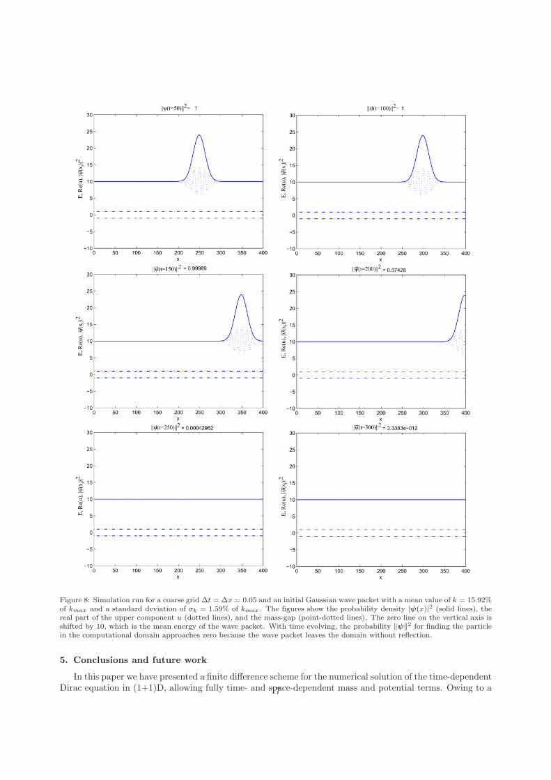
Figure 8: Simulation run for a coarse grid ∆t = ∆x = 0.05 and an initial Gaussian wave packet with a mean value of k = 15.92%of kmax and a standard deviation of σk = 1.59% of kmax. The figures show the probability density |ψ(x)|2 (solid lines), thereal part of the upper component u (dotted lines), and the mass-gap (point-dotted lines). The zero line on the vertical axis isshifted by 10, which is the mean energy of the wave packet. With time evolving, the probability ‖ψ‖2 for finding the particlein the computational domain approaches zero because the wave packet leaves the domain without reflection.

5. Conclusions and future work

In this paper we have presented a finite difference scheme for the numerical solution of the time-dependentDirac equation in (1+1)D, allowing fully time- and space-dependent mass and potential terms. Owing to a17

Figure 9: Time dependence of the spinor norm ‖ψ(t)‖ of the simulation run shown in Fig. 8: logarithmic scale (left) and linearscale (right).

combined staggering of the grid both in space and time, unphysical additional Dirac cones are avoided and,for the special case of the Weyl equation, the linear dispersion is preserved exactly for all wave numberssupported by the grid. In the case of finite mass and/or potential terms the dispersion relation improvesfor all wave numbers, approaching the continuum dispersion relation exactly, when the grid is refined. Thisis a relevant feature when modeling Dirac fermions on a lattice, such as Dirac fermions propagating ontopological insulator surfaces, graphen, or in quantum spin Hall states. The electromagnetic potentialsaccounting for an external electromagnetic field are included in gauge invariant fashion. A stability analysisof the scheme was performed and a functional, exactly conserved by the scheme, was identified. It providesa valid norm for the spinor on the proposed staggered grid.

Furthermore, we have derived exact DTBCs to close the finite difference scheme for constant mass andpotential in the boundary regions. With these BCs one is in the position to deal with particle transportscenarios and to account for the multi-band nature of the Dirac equation which may cause inter-bandtransfer rather than quantum confinement. For completeness, DTBCs were also derived for the (1+1) Dirac(differential) equation in Schrodinger form.

Using the norm for a measure, numerical simulations of Gaussian wave packets show them leaving thecomputational domain without reflections (with an error below computer precision), thus verifying thequality of the DTBCs numerically. The importance of a faithful representation of the energy-momentumdispersion relation, in particular, avoiding fermion doubling, is exemplified in numerical simulations.

The assumptions of constant mass and potential on the exterior domain can be loosened. It is howeverdesirable that an analytic solution on the discrete exterior domain can be found. The case of purely time-dependent exterior potential can be treated by using a proper phase change of the spinor. Initial conditionsfor which the initial wave packet is not compactly supported on the computational domain can be handledas well, leading to inhomogeneous terms in the boundary conditions. There are various ways to extend theproposed leap-frog scheme to the (2+1)D Dirac equation where it retains many of its attractive features[45, 46, 49]. The formulation of DTBCs for the (2+1)D Dirac equation in the spirit of this paper is thesubject of future work [49].

In view of existing work on non-linear versions of the Dirac equation accounting, for example, for self-interaction corrections in a single equation, we wish to point out that a self-consistent treatment of sucheffects can be treated readily (and in more generality) within the present approach based on the stan-dard Dirac equation and a parallel self-consistent update of the effective electromagnetic potentials. In asemi-classical picture, for example, the latter may be accomplished within Maxwell’s theory for the elec-

18

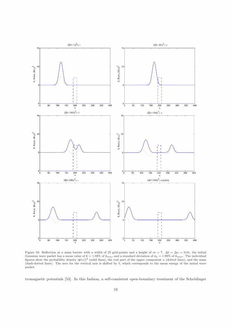
Figure 10: Reflection at a mass barrier with a width of 25 grid-points and a height of m = 7. ∆t = ∆x = 0.01, the initialGaussian wave packet has a mean value of k = 1.59% of kmax and a standard deviation of σk = 1.99% of kmax. The individualfigures show the probability density |ψ(x)|2 (solid lines), the real part of the upper component u (dotted lines), and the mass(dash-dotted lines). The zero for the vertical axis is shifted by 5, which corresponds to the mean energy of the initial wavepacket.

tromagnetic potentials [53]. In this fashion, a self-consistent open-boundary treatment of the Schrodinger

19

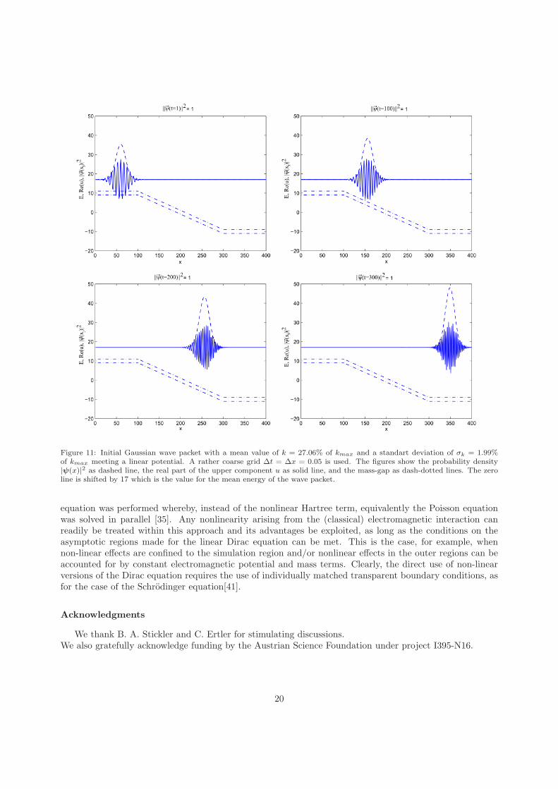
Figure 11: Initial Gaussian wave packet with a mean value of k = 27.06% of kmax and a standart deviation of σk = 1.99%of kmax meeting a linear potential. A rather coarse grid ∆t = ∆x = 0.05 is used. The figures show the probability density|ψ(x)|2 as dashed line, the real part of the upper component u as solid line, and the mass-gap as dash-dotted lines. The zeroline is shifted by 17 which is the value for the mean energy of the wave packet.

equation was performed whereby, instead of the nonlinear Hartree term, equivalently the Poisson equationwas solved in parallel [35]. Any nonlinearity arising from the (classical) electromagnetic interaction canreadily be treated within this approach and its advantages be exploited, as long as the conditions on theasymptotic regions made for the linear Dirac equation can be met. This is the case, for example, whennon-linear effects are confined to the simulation region and/or nonlinear effects in the outer regions can beaccounted for by constant electromagnetic potential and mass terms. Clearly, the direct use of non-linearversions of the Dirac equation requires the use of individually matched transparent boundary conditions, asfor the case of the Schrodinger equation[41].

Acknowledgments

We thank B. A. Stickler and C. Ertler for stimulating discussions.We also gratefully acknowledge funding by the Austrian Science Foundation under project I395-N16.

20

Appendix A. Analytic derivation of the convolution coefficients τ(n)1 for the general case

We shall first consider the case m = V = 0 where (54) reads

τ1(z) = 1 +1

2r2z(z − 1)2 − z − 1

2r2z

√

z2 − 2µz + 1 ,

with µ := 1 − 2r2. Here, the branch of the square root is chosen such that τ1(z) = O(|z|−1) as z → ∞.Using

Z−1

{√

z2 − 2µz + 1

z

}

= Pn−2(µ)− 2µPn−1(µ) + Pn(µ) =1

n[Pn−2(µ)− µPn−1(µ)] , (A.1)

where Pn denotes the Legendre polynomials (with the convention P−1 = P−2 := 0), we obtain

τ(n)1 = (1− 1

r2)δn0 +

1

2r2δn1 − 1

2r2

[

Pn+1(µ)− (2µ+ 1)(Pn(µ)− Pn−1(µ))− Pn−2(µ)]

, n ≥ 0 .

And this simplifies to τ(n)1 = δn1 for r = 1.

Next we shall discuss the general case with m, V ∈ R. Here we have

τ1(z) = 1 +c

2z− 1

2z

√c√c+ 4z ,

where c(z) := z c(z) = αz2+βz+γ is a quadratic polynomial given by (52). Using again (A.1), both square

root factors can be inverse Z-transformed. And the explicit formula for the coefficients τ(n)1 would then

involve a discrete convolution.

But we shall proceed differently here and rather derive a recursion relation for τ(n)1 (similar as in §3 of

[50]). A lengthy, but straightforward computation shows that τ1(z) := z τ1(z) satisfies the inhomogeneousdifferential equation

c(c+ 4z) τ ′1 − [2α2z3 + 3α(β + 2)z2 + (β2 + 4β + 2αγ)z + (β + 2)γ] τ1 = 2z(γ − αz2) . (A.2)

Since all coefficients in (A.2) are polynomials we shall use the Laurent series of τ1, i.e. τ1 =∑∞

n=0 s(n)z−n,

with τ(n)1 = s(n−1). A comparison of the coefficients then yields:

s(0) =1

α, s(1) = −β + 2

α2, s(2) =

β2 + 4β + 5− αγ

α3,

and the exact recursion

(n+5)α2s(n+3)+(2n+7)α(β+2)s(n+2)+(n+2)(β2+4β+2αγ)s(n+1)+(2n+1)(β+2)γs(n)+(n−1)γ2s(n−1) = 0 ,

for n ≥ 0 with the convention s(−1) := 0.

21

Appendix B. Gauge-invariant introduction of the electromagnetic vector potential

Dirac equation Eq. (1) sofar has been written for a charged massive particle in a scalar potential. For ageneral account of external electromagnetic fields and/or self-interaction both scalar and vector potential areneeded. A gauge invariant introduction of the electromagnetic vector potential A(x, t) is executed by replac-

ing the complex 2-spinor ψ =

(u(x, t)v(x, t)

)

in Eq. (1) by ψ(x, t) exp{−ia(x, t)} =

(u(x, t) exp{−ia(x, t)}v(x, t) exp{−ia(x, t)}

)

,

with[51, 52]

a(x, t) :=q

~c

∫ x

xo

dyA(y, t) .

Position xo is arbitrary but constant. Under this Peierls substitution the canonical momentum p := ~

i∂∂x

in Eq. (1) is replaced by the kinetic momentum p − qcA(x, t) =

~

i∂∂x − q

cA(x, t). Under local gauge trans-

formation A(x, t) → A(x, t) + ∂∂xΛ(x, t), Φ(x, t) → Φ(x, t)− ∂

c∂tΛ(x, t), the spinor acquires the phase factorexp{−i q

~c (Λ(x, t)− Λ(xo, t))}, and the electromagnetic fields E and B remain invariant.

Here it should be pointed out that in a (1+1)D model, orbital forces are confined to one spatial direc-tion (i.e., x), while non-vanishing torque on the spin degree of freedom (in a Larmor term) arising fromAx(x, t) = A(x, t) requires a non-vanishing B field component in the plane orthogonal to x. Note, however,that the two-component nature of an effective Dirac model may not arise from the spin degree of freedom.Most notable example in 2+1D is graphene [3]. This shows that the physical interpretation of the effectiveDirac equation and the way an electromagnetic field couples to the system is determined by the underlyingbasic theory.

We now discuss the consequences of the Peierls substitution on the leap-frog scheme Eqs. (20) and (21).Again, we have V (x, t) = −Φ(x, t), and for any grid point xj , tn we define anj := a(xj , tn). The leap-frogscheme for non-zero vector potential is obtained by the substitution

un−1/2j → u

n−1/2j := u

n−1/2j exp{−ian−1/2

j } ,vnj−1/2 → vnj−1/2 := vnj−1/2 exp{−ianj−1/2} . (B.1)

Likewise, the stability analysis for zero vector potential detailed above can immediately be extended to thecase of a non-vanishing vector potential by the substitution Eq. (B.1) and noting that the vector potentialA(x, t) is real valued. Hence, a strictly conserved functional En

r is identified by this substitution applied tothe expression for En

r in Eq. (42) for arbitrary time t and space x dependent m,V,A ∈ R. It follows thatthe scheme remains stable for all r = ∆t/∆x ≤ 1.

Expressed in terms of spinor components u and v the scheme in presence of an external electromagneticpotential takes the form

f+(an+1/2j , a

n−1/2j )

[

un+1/2j − u

n−1/2j

∆t+ i

(

mnj − V n

j −an+1/2j − a

n−1/2j

∆t

)un+1/2j + u

n−1/2j

2

]

+ if−(an+1/2j , a

n−1/2j )(mn

j − V nj )un+1/2j − u

n−1/2j

2

+ f+(anj+1/2, anj−1/2)

[

(Dvn)j∆x

− ianj+1/2 − anj−1/2

∆x

vnj+1/2 + vnj−1/2

2

]

= 0 , (B.2)

22

f+(an+1j−1/2, a

nj−1/2)

[vn+1j−1/2 − vnj−1/2

∆t− i(m

n+1/2j−1/2 + V

n+1/2j−1/2 +

an+1j−1/2 − anj−1/2

∆t)vn+1j−1/2 + vnj−1/2

2

]

− if−(an+1j−1/2, a

nj−1/2)(m

n+1/2j−1/2 + V

n+1/2j−1/2 )

vn+1j−1/2 − vnj−1/2

2

+ f+(an+1/2j , a

n+1/2j−1 )

[

(Dun+1/2)j−1/2

∆x− i

an+1/2j − a

n+1/2j−1

∆x

un+1/2j + u

n+1/2j−1

2

]

= 0 . (B.3)

Here we have used the definition f±(a1, a2) := (e−ia1±e−ia2)/2. As in the main text, we set c = ~ = 1 = −q.For slowly varying vector potential (or within first order in ∆t) one may approximate these equations by

un+1/2j − u

n−1/2j

∆t+ i(mn

j − V nj )un+1/2j + u

n−1/2j

2

+

[(Dvn)j∆x

+ iAnj

vnj+1/2 + vnj−1/2

2

]

= 0 , (B.4)

vn+1j−1/2 − vnj−1/2

∆t− i(m

n+1/2j−1/2 + V

n+1/2j−1/2 )

vn+1j−1/2 + vnj−1/2

2

+

[(Dun+1/2)j−1/2

∆x+ iA

n+1/2j−1/2

un+1/2j + u

n+1/2j−1

2

]

= 0 . (B.5)

Here we have used the following abbreviations on the two sub-lattices: V nj := V n

j +an+1/2j −a

n−1/2j

∆t and

Vn+1/2j−1/2 = V

n+1/2j−1/2 +

an+1

j−1/2−an

j−1/2

∆t denote the net scalar potential associated with the E field after introduction

of the vector potential, and Anj =

anj−1/2−an

j+1/2

∆x and An+1/2j−1/2 =

an+1/2j−1

−an+1/2j

∆x are the vector potential, as

defined by symmetric spatial derivatives of a(x, t). Note that we use q = −1.The approximate scheme (B.4) and (B.5) may have been guessed directly by inspection of Eqs. (20) and

(21). Going the present way, however, not only has given the way for precise implementation of the vectorpotential into the latter but also has taken care of the stability analysis for this general case. Finding anexactly conserved functional for the approximate scheme is complicated by the fact that the vector potentialleads to additional coupling between the spinor components u and v.

23

[1] W. Greiner, Relativistic quantum mechanics: wave equations, 3rd ed., Springer Berlin (2000).[2] B. Thaller, The Dirac Equation, Springer Berlin (1992).[3] A. H. Castro-Neto, F. Guinea, N. M. R. Peres, K. S. Novoselov and A. K. Geim, The electronic properties of graphene,

Reviews of Modern Physics 81 (2009) 109-162.[4] B. A. Bernevig, T. L. Hughes, and S. C. Zhang, Quantum Spin Hall Effect and Topological Phase Transition in HgTe

Quantum Wells, Science 314 (2006) 1757-1761.[5] X. L. Qi and S. C. Zhang, Topological insulators and superconductors, Reviews of Modern Physics 83 (2011) 1057-1110.[6] L. Lamata, J. Casanova, R. Gerritsma, C. F. Roos, J. J. Garcıa-Ripoll and E. Solano, Relativistic quantum mechanics

with trapped ions, New Journal of Physics 13 (2011) 1367-2630.[7] D. Witthaut, T. Salger, S. Kling, C. Crossert and M. Weitz, Effective Dirac dynamics of ultracold atoms in bichromatic

optical lattices, Physical Review A 84 (2011) 033601.[8] N. Szpak and R. Schutzhold, Optical lattice quantum simulator for quantum electrodynamics in strong external fields:

spontaneous pair creation and the Sauter-Schwinger effect, New Journal of Physics 14 (2012) 035001.[9] L. H. Ryder, Quantum field theory, 2nd ed., University Press Cambridge (1996).

[10] B. Thaller, Advanced Visual Quantum Mechanics, Springer New York (2005).[11] O. Busic, N. Grun, and W. Scheid, A new treatment of the fermion doubling problem, Physics Letters A 254 (1999)

337-340.[12] R. Stacey, Eliminating lattice fermion doubling, Physical Review D 26, (1982) 468-472.[13] J. Tworzydlo, C. W. Groth, and C. W. J. Beenakker, Finite difference method for transport properties of massless Dirac

fermions, Physical Review B 78 (2008) 235438.[14] C. Muller, N. Grun, and W. Scheid, Finite element formulation of the Dirac equation and the problem of fermion doubling,

Physics Letters A 242 (1998) 245-250.[15] K. Momberger and A. Belkacem, Numerical treatment of the time-dependent Dirac equation in momentum space for

atomic processes in relativistic heavy-ion collisions, Physical Review A 53 (1996) 1605-1622.[16] J. W. Braun, Q. Su, and R. Grobe, Numerical approach to solve the time-dependent Dirac equation, Physical Review A

59 (1999) 604-612.[17] G. R. Mocken and C. H. Keitel, Quantum dynamics of relativistic electrons, Journal of Computational Physics 199 (2004)

558-588.[18] F. Fillion-Gourdeau, E. Lorin, and A. D. Bandrauk, Numerical Solution of the Time-Dependent Dirac Equation in Coor-

dinate Space without Fermion-Doubling, Comp. Phys. Comm. 183 (2012) 1403-1415.[19] H. B. Nielsen and M. Ninomiya, A no-go theorem for regularizing chiral fermions, Physics Letters B 105 (1981) 219-223.[20] J. Xu, S. Shao, and H. Tang, Numerical methods for non-linear Dirac equation, J. Comp. Phys. 245 (2013) 131-149.[21] M. Soler, Classical, stable, nonlinear spinor field with positive rest energy, Phys. Rev. D 1 (1970) 27662769.[22] S. Coleman, Quantum sine-Gordon equation as the massive Thirring model, Phys. Rev. D 11 (1975) 20882097.[23] A. Alvarez and B. Carreras, Interaction dynamics for the solitary waves of a nonlinear Diracmode, Physics Letters 86A

(1981) 327-332.[24] A. Alvarez, P.Y. Kuo, L. Vzquez, The numerical study of a nonlinear one-dimensional Dirac equation, Appl. Math.

Comput. 13 (1983) 115.[25] A. Alvarez, Linearized CrankNicholson scheme for nonlinear Dirac equations, J. Comput. Phys. 99 (1992) 348350.[26] P. Gordon, Nonsymmetric difference equations, SIAM J. Appl. Math. 13 (1965) 667673.[27] J. De Frutos, J.M. Sanz-Serna, Split-step spectral schemes for nonlinear Dirac systems, J. Comput. Phys. 83 (1989) 407423.[28] Z.Q. Wang, B.Y. Guo, Modified Legendre rational spectral method for the whole line, J. Comput. Math. 22 (2004) 457474.[29] J.L. Hong, C. Li, Multi-symplectic RungeKutta methods for nonlinear Dirac equations, J. Comput. Phys. 211 (2006)

448472.[30] S.H. Shao, H.Z. Tang, Higher-order accurate RungeKutta discontinuous Galerkin methods for a nonlinear Dirac model,

Discrete Cont. Dyn. Syst. B 6 (2006) 623640.[31] H. Wang, H. Tang, An efficient adaptive mesh redistribution method for a non-linear Dirac equation, Journal of Compu-

tational Physics 222 (2007) 176193.[32] V. A. Baskakov and A.V. Popov, Implementation of transparent boundaries for numerical solution of the Schrodinger

equation, Wave Motion 14 (1991) 123-128.[33] B. Mayfield, University of Rhode Island, Providence, Ph.D. thesis (1989).[34] A. Arnold, M. Ehrhardt, and I. Sofronov, Discrete transparent boundary conditions for the Schrodinger equation: fast

calculation, approximation, and stability, Communications in Mathematical Sciences 1 (2003) 501-556.[35] M. A. Talebian and W. Potz, Open boundary conditions for a time-dependent analysis of the resonant tunneling structure,

Applied Physics Letters 69 (1996) 1148-1150.[36] W. Potz, Scattering theory for mesoscopic quantum systems with non-trivial spatial asymptotics in one dimension, Journal

of Mathematical Physics 36 (1995) 1707.[37] A. Zisowsky, A. Arnold, M. Ehrhardt, and T. Koprucki, Discrete transparent boundary conditions for transient kp-

Schrodinger equations with application to quantum heterostructures, Journal of Applied Mathematics and Mechanics 11(2005) 793-805.

[38] I. Alonso-Mallo and N. Reguera, Weak Ill-Posedness of Spatial Discretizations of Absorbing Boundary Conditions forSchrodinger-Type Equations, SIAM Journal on Numerical Analysis 40 (2002) 134-158.

[39] C. Lubich and A. Schadle, Fast Convolution for Nonreflecting Boundary Conditions, SIAM Journal on Scientific Computing24 (2002) 161-182.

[40] C. W. Rowley and T. Colonius, Discretely Nonreflecting Boundary Conditions for Linear Hyperbolic Systems, Journal of

24

Computational Physics 157 (2000) 500-538.[41] X. Antoine, A. Arnold, C. Besse, M. Ehrhardt, and A. Schadle, A Review of Transparent and Artificial Boundary

Conditions Techniques for Linear and Nonlinear Schroodinger Equations, Communications in Computational Physics 4(2008) 729-796.

[42] E. Hairer, C. Lubich, and G. Wanner, Geometric numerical integration illustrated by the Stormer/Verlet method, ActaNumerica 12 (2003) 399-450.

[43] A. Borzı and E. Decker, Analysis of a leap-frog pseudospectral scheme for the Schrodinger equation, Journal of Compu-tational and Applied Mathematics 193 (2006) 65-88.

[44] A. Arnold, Mathematical concepts of open quantum boundary conditions, Transp. Theory Stat. Phys. 30/4-6 (2001)561-584.

[45] R. Hammer and W. Potz, Staggered-grid leap-frog scheme for the (2+1)D Dirac equation, accepted in Computer PhysicsCommunications, http://dx.doi.org/10.1016/j.cpc.2013.08.013

[46] R. Hammer, C. Ertler, and W. Potz, Dirac fermion wave guide networks on topological insulator surfaces, arXiv:1205.6941(2012).

[47] R. Hammer, C. Ertler, and W. Potz, Solitonic Dirac fermion wave guide networks on topological insulator surfaces, Appl.Phys. Lett. 102, (2013) 193514-1 - 193514-4.

[48] R. Hammer and W. Potz, Dynamics of domain-wall Dirac fermions on a topological insulator: a chiral fermion beamsplitter, arXiv:1306.6139

[49] A manuscript showing the extension of the (1+1)D scheme to a (2+1)D scheme which conserves the monotone dispersionrelation (= having a single Dirac cone) is in preparation.

[50] M. Ehrhardt and A. Arnold, Discrete Transparent Boundary Conditions for the Schrodinger Equation, Revista di Matem-atica della Universita di Parma 6/4 (2001) 57-108.

[51] R. Peierls, Zur theorie des diamagnetismus von leitungselektronen, Z. Phys. 80 (1933) 763-791.[52] M. Graf und P. Vogl, Electromagnetic fields and dielectric response in empirical tight-binding theory, Phys. Rev. B 51

(1995) 49404949, and references therein.[53] J.D. Jackson, Classical Electrodynamics, 2nd edition (Wiley, New York, 1975).

25