Embed Size (px)
Citation preview

iii
VISUAL AND PERSISTENT
CO-DESIGN MODELING FOR NETWORK SYSTEMS
by
Weilong Hu
A Dissertation Presented in Partial Fulfillment of the Requirements for the Degree
Doctor of Philosophy
ARIZONA STATE UNIVERSITY
August 2007

iv
ABSTRACT
Network systems are challenging to model because of the complexity inherent in
the software and hardware designs as well as the numerous ways that they may be
synthesized. A desired goal towards describing computer network systems is: visual and
persistent modeling of combined software and hardware components. Furthermore, the
co-design modeling approach is poised to provide advanced capabilities to support
separate and combined specifications of software and hardware layers of network
systems.
The Distributed Object Computing (DOC) approach offers an abstraction for
modeling any network system in terms of logical specification of software and hardware
components and the mappings of the former to the latter. The abstraction defines software
(Distributed Cooperative Objects (DCO)), hardware (Loosely Coupled Network (LCN)),
and Object System Mapping (OSM) models. These models can be described and
simulated in DEVS/DOC – a DEVS-based environment for simulating DOC models.
However, neither DOC nor DEVS offers visual and persistent model concepts and
methods. In contrast, Scalable Entity Structure Modeler (SESM) framework supports a
unified logical, visual, and persistence component-based model development for
specifying families of complex system designs, but it lacks direct support for co-design.
Considering the limitations of DEVS/DOC, SESM, and other modeling
approaches, this dissertation develops an approach called SESM/DOC where logical co-
design model specifications can be developed visually and stored in relational databases.
This approach introduces visual and persistent co-design capabilities for describing a
family of logical models for network systems. The SESM/DOC has been devised to

v
support consistent logical, visual, and persistent modeling for the DCO, LCN, and OSM
models. A prototype has been developed (i) to support separate visual working sections
for software and hardware modeling and their synthesis, (ii) to store logical co-design
models, and (iii) to automatically generate partial equivalent DEVS/DOC models. For the
purposes of demonstration, an example of search engine systems is considered. The
example is modeled in SESM/DOC and simulated in DEVS/DOC. The role of the
proposed co-design modeling approach and its application for development of network
system designs is examined and select future research directions are briefly described.

vi
ACKNOWLEDGMENTS
I would like to thank my advisor, Dr. Hessam Sarjoughian, for introducing me to
the research area of modeling and simulation, for insight advice and good guidance, for
friendship and continuous inspirations.
Sincerely thanks to my other committee members, Dr. James Collofello, Dr.
Susan Urban, and Dr. Guoliang Xue, for their time and efforts in reviewing my Ph.D.
proposal and dissertation and in the discussions and help.
Thanks to the National Science Foundation (DMI-0075557 and DMI-0432439),
Intel Research Council, and the Boeing Company, for partial support of this research.

vii
TABLE OF CONTENTS
Page
LIST OF TABLES ………………………………………………………………………..x
LSIT OF FIGURES……………………………………………………………………...xii
CHAPTER
1 INTRODUCTION ...................................................................................................... 1
1.1 The Problem........................................................................................................ 1
1.2 Current Approaches and Challenges................................................................... 3
1.3 Contributions....................................................................................................... 8
1.4 Dissertation Outline .......................................................................................... 10
2 BACKGROUND AND RELATED WORKS .......................................................... 13
2.1 System Engineering Overview ......................................................................... 13
2.1.1 System Design .......................................................................................... 15
2.1.2 Simulation-based System Design ............................................................ 17
2.2 Modeling and Simulation Concepts.................................................................. 19
2.2.1 System Formalisms................................................................................... 21
2.2.2 Basic Model Types ................................................................................... 22
2.2.3 System Morphisms.................................................................................... 24
2.2.4 Verification and Validation....................................................................... 26
2.3 Software Engineering ....................................................................................... 27
2.3.1 Use of Software Engineering in Simulation Tools ................................... 31
2.4 Model-Driven Engineering ............................................................................... 34
2.4.1 Model-Integrated Computing (MIC) ........................................................ 36

viii
2.4.2 Model-Driven Architecture (MDA).......................................................... 38
2.4.3 Model Design Methods and Tools ............................................................ 40
2.5 Summary........................................................................................................... 51
3 MODELING AND SIMULATION APPROACHES AND TOOLS ....................... 52
3.1 Scalable Entity Structure Modeler Concepts and Approach ............................ 52
3.1.1 Framework and Related Modeling and Simulation Architecture ............. 54
3.1.2 Model Example......................................................................................... 56
3.2 Discrete Event System Specification................................................................ 61
3.2.1 Concepts and Approach ............................................................................ 61
3.2.2 DEVSJAVA Simulation Environment ..................................................... 63
3.2.3 Simulation Model Example ...................................................................... 68
3.3 Distributed Object Computing Modeling Approach ........................................ 70
3.3.1 Abstract Model.......................................................................................... 70
3.3.2 DEVS Realization of DOC ....................................................................... 75
3.3.3 Network System Simulation with DEVS/DOC ........................................ 76
3.3.4 Discussion of Network System Simulation Tools .................................... 81
3.4 Summary........................................................................................................... 83
4 COMPONENT-BASED LAYERED STRUCTURE MODELING APPROACH
FOR CO-DESIGN NETWORK SYSTEMS .................................................................... 85
4.1 Co-Design Modeling Approach for Network Systems..................................... 85
4.2 Layered Structure Decomposition for Network Systems ................................. 88
4.2.1 Model Types in Scalable Entity Structure Modeling................................ 88
4.2.2 Constraints in Distributed Computing Modeling...................................... 93
ix
4.2.3 Layered Structure Decomposition for Distributed Computing Systems .. 94
4.3 Model Bases for Layered Structure Modeling................................................ 100
4.3.1 Model Types for Co-design .................................................................... 102
4.3.2 Network System Model Constraints ....................................................... 104
4.4 Summary......................................................................................................... 107
5 CO-DESIGN VISUAL AND PERSISTENT MODELS PRESENTATION FOR
NETWORK SYSTEMS.................................................................................................. 109
5.1 Visual Modeling ............................................................................................. 109
5.1.1 Model Components................................................................................. 110
5.1.2 Model Relationship................................................................................. 111
5.1.3 Tree Structure and Block Diagram Views .............................................. 114
5.1.4 Multiple Layer Model Representation .................................................... 116
5.2 Model Persistence ........................................................................................... 117
5.3 Summary......................................................................................................... 125
6 DISTRIBUTED CO-DESIGN MODELING EXAMPLE...................................... 127
6.1 The Search Engine Network System Problem................................................ 127
6.2 Model Design.................................................................................................. 129
6.2.1 Primitive and Composite Components ................................................... 129
6.2.2 Hardware Model ..................................................................................... 130
6.2.3 Software Model....................................................................................... 139
6.2.4 Object System Mapping Design ............................................................. 142
6.3 V&V Based on Model Types and Model Constraints .................................... 143
6.4 Semi-automatic Simulation Code Generation ................................................ 145
x
6.5 System Analysis.............................................................................................. 147
6.5.1 System Simulation Experiments Set-Up................................................. 148
6.5.2 Alternative Hardware Network Analysis................................................ 149
6.5.3 Alternative Software Network Analysis ................................................. 152
6.6 Summary.......................................................................................................... 156
7 CONCLUSION....................................................................................................... 158
7.1 A Comparison of SESM/DOC......................................................................... 158
7.1.1 Modeling and Simulation Environments ................................................ 158
7.1.2 Relating SESM/DOC with Other Network System Modeling ............... 161
7.1.3 SESM/DOC and V&V............................................................................ 164
7.2 Summary.......................................................................................................... 165
7.3 Future Works ................................................................................................... 170

xi
LIST OF TABLES
Table Page
1. Design Process Functions ............................................................................................. 16
2. System Knowledge Hierarchy ...................................................................................... 19
3. System Specification Hierarchy.................................................................................... 20
4. System Morphism Precondition in System Specification Hierarchy............................ 24
5. SESM Structural complexity Metrics ........................................................................... 59
6. XML and DEVSJAVA Code Generated In SESM....................................................... 60
7. DEVSJAVA 3.0 Modules............................................................................................. 64
8. DEVSJAVA AntiVirusSystem Source Code................................................................ 68
9. DEVSDOC AntiVirusSystem Source Code ................................................................. 77
10. Selected Hardware, Software, and Experimentation Components ............................. 80
11. Multiple Model Bases for Distributed Object Computing System........................... 102
12. OSM Mapping Table ................................................................................................ 122
13. Software Model Type Table ..................................................................................... 123
14. Hardware Model Type Table .................................................................................... 124
15. SESM/DOC Network Models................................................................................... 130
16. Generated XML File ................................................................................................. 145
17. Generated DEVS/DOC Code.................................................................................... 146
18. Experiments Settings ................................................................................................ 148
19. Search Requests Distribution.................................................................................... 150
20. Comparison of selected general purpose modeling and simulation tools................. 159
21. Comparison of network system modeling and simulation tools............................... 161
xii
22. Modeling and Simulation Supports in Network Protocol Layers............................. 163

xiii
TABLE OF FIGURES
Figure Page
1. System Design with Modeling and Simulation ............................................................ 18
2. State Transitions in Homomorphic Systems................................................................. 25
3. Software Engineering Layers........................................................................................ 28
4. Motivation of MVC ...................................................................................................... 32
5. MVC Example .............................................................................................................. 33
6. Model-Integrated Computing Life Cycle...................................................................... 37
7. Model-Driven Architecture Procedure ......................................................................... 39
8. Basic SESM ER Diagram ............................................................................................. 54
9. SESM Architecture ....................................................................................................... 55
10. Modeling and Simulation with SESM ........................................................................ 56
11. Visual Model of detectUnit and killUnit .................................................................... 57
12. Template Model of WorkStation Composite Model .................................................. 58
13. Persistent Model.......................................................................................................... 58
14. DEVSJAVA 2.63 Container Specification ................................................................. 65
15. GenCol Container Specification ................................................................................. 65
16. viewableAtomic and viewableDigraph....................................................................... 66
17. Simulator Utilities....................................................................................................... 66
18. Graphical View of An Atomic Model in DEVSJAVA 3.0......................................... 67
19. AntiVirusSystem Simulation View in DEVSJAVA GUI........................................... 69
20. Distributed Object Computing Approach ................................................................... 71
21. DEVS/DOC Structure................................................................................................. 76

xiv
22. AntiVirus System Example with DEVS/DOC ........................................................... 77
23. Shared Bus Topology.................................................................................................. 79
24. Distributed Co-Design Network System .................................................................... 86
25. Conceptual Approach for SESM/DOC....................................................................... 96
26. Model Coupling and Model Mapping ...................................................................... 100
27. Block Diagram Visual Model ................................................................................... 110
28. Link Group Model .................................................................................................... 111
29. The Non-arrowed Segment Line for Model Connection .......................................... 113
30. OSM Model .............................................................................................................. 113
31. Alternative OSM Model ........................................................................................... 114
32. SESM Model Tree Structure..................................................................................... 115
33. Model Specialization ................................................................................................ 115
34. Multiple Sections for Visual Modeling..................................................................... 116
35. DOC Data Schema - Kernel...................................................................................... 118
36. DOC Data Schema – Ports, Coupling, State Variable and Statistics........................ 119
37. DOC Data Schema – OSM Model............................................................................ 120
38. Search Engine Network System................................................................................ 127
39. Primitive Hardware Model Development................................................................. 131
40. Adding Hardware Components into Hardware Group Model.................................. 132
41. Hardware Group Model ............................................................................................ 133
42. “H” Style Hardware Layer........................................................................................ 134
43. Instance Template Model Tree Structure for “H” Style Hardware Model ............... 135
44. “I” Style Network System......................................................................................... 135

xv
45. “I” Style Hardware Layer ......................................................................................... 136
46. Structural complexity Metrics for “H” Style System .............................................. 137
47. Structural complex Metrics for “I” Style System ..................................................... 137
48. Hardware Specialization ........................................................................................... 138
49. Adding State Variables for Hardware Specialization ............................................... 139
50. Adding Software Models into Software Layer Model.............................................. 140
51. Software Model Coupling......................................................................................... 141
52. “H” Style OSM Model.............................................................................................. 143
53. “I” Style OSM Model ............................................................................................... 143
54. Experiments Boundary.............................................................................................. 149
55. Data Analysis for “I” Style and “H” Style................................................................ 152
56. Star Network Topology............................................................................................. 153
57. Data Analysis for Alternative Software Applications .............................................. 156
58. Hybrid Reference Model for Computer Network Protocol Stack ............................ 162

1 INTRODUCTION
1.1 The Problem
Networks of computer hardware and software systems have grown rapidly in their
complexity and scale due to advances in computer science and software engineering.
Examples of such systems are search engines, global information systems, and command
and control engineering enterprises. These systems are complex and are stretching the
capabilities of the most advanced analysis and design approaches and their state-of-the-
art tools.
Integral to building such systems is the desire to increase the performance-to-cost
ratio. A key phenomenon is the continuing shift from central computing technologies to
their distributed counterparts. One aspect of these modern network systems is that their
highly intricate dynamics are rooted in architectural design choices, constraints, and the
technologies that are used to build them. The difficulties of designing a large-scale and
complex network system (e.g., an enterprise system supporting large-scale distributed
event processing in the domain of information management) provide challenging research
questions for simulation-based system modeling. Developing solutions to these questions
is considered important fundamental research with key implications in the engineering of
network systems for commercial and government uses.
Another aspect of a modern network system is that software components may be
mapped onto alternative networked hardware components. Therefore, a basic concept in
computer-aided system design is to distinguish between software and hardware

2
components while allowing the flexibility to synthesize these different components to
create the desired system architectures.
To create network systems and in particular support simulation-based system
design, it is advantageous to bring together concepts, methods, and practices from
modeling and simulation, software engineering, and system engineering. Modeling and
simulation has been widely applied in system engineering which provides an overarching
framework for defining, developing and deploying systems (Sage & Armstrong, 2000).
Analysis and design are essential parts of system engineering as well as software
engineering. Today’s system engineers must handle systems that are by orders of
magnitude more complex than those they could deal with just a few years ago. In order to
develop design and analysis models for network systems, a system has to be decomposed
hierarchically into its comparatively simpler sub-systems (or components). Intelligent
decomposition of a system is prerequisite to success in developing network systems.
Furthermore, the design of the individual components is generally difficult.
Decomposition of a system into a set of cohesive software and hardware components
remains challenging for scientists and engineers. Similarly, it is difficult to select and fit a
component appropriately into a system’s architecture. The structure and behavior of the
components of a system affect the overall system and, conversely, the structure and
behavior of the system influences the choices of the components.
The above problems are conceptually similar to those that have been considered
for embedded systems. To allow combined model-based software and hardware design,
the concept of co-design was developed. It allows designers to simultaneously account

3
for requirements that span to both the software and to the hardware on which the software
is expected to execute. Embedded systems have their own unique requirements but also
share some basic concepts with those of distributed network systems. The separation of
embedded software and hardware and the successful application of co-design offer a
strong case for their use in architecting network systems. Indeed, a co-design
methodology has been developed for simulation-based analysis and design of systems.
The approach supports system architects in simulation and to in evaluation of design
choices. Engineers can try different designs with the convenience and systematic use of
co-design simulation models that separate and integrate software and hardware parts of
systems. Enabling the design of network systems, however, requires co-design
capabilities that are rigorous and simple to use.
1.2 Current Approaches and Challenges
Engineering of the above network system architectures is of interest to analysts
and designers alike. System architects must deal with the complexity of network systems
and the limitations of existing modeling approaches from both software and simulation
design perspectives. To overcome the restrictions and inadequacies of techniques and
methods for describing a system’s structure and behavior, researchers are pursuing
solutions that can simplify system design, such as system modeling and simulation.
A model is a set of instructions, rules, equations, or constraints to present the
structure or behavioral properties of a system (Blanchard, 2004). Simulation makes one
system (model or models) do the essential work of another system. There are many

4
reasons for using modeling and simulation in system design (Wymore, 1993). Modeling
and simulation play an important role before the system is built, while the system is being
built, and after the system is completed. For large-scale and complex systems, modeling
and simulation is particularly important because testing these kinds of real systems is
often not possible and/or is expensive. One school of research is primarily interested in
software and system modeling such as MDD (Model-Driven Design) (Muth, 2005), UML
(Object Management Group, 2007), Service Oriented Architecture (Anand,
Pandmanabhuni, & Ganesh, 2005), Grid Computing (Darema 2005), SysML(Hause,
Thom, & Moore, 2005), and Raphosady (Gery, Harel, & Palachi, 2002). Another school
of research is pursuing simulation-based approaches with strong emphasis on developing
models that can be simulated dynamically, such as SMART (simulation and modeling for
acquisitions, requirements, and training) (Lunceford, 2002), and DEVS (Discrete Event
System Specification) (Sarjoughian & Cellier, 2001; Zeigler, Praehofer, & Kim, 2000).
Some of these approaches are advocating developing simulation models that can be
mapped (semi-)automatically to specifications that can serve as blueprint for engineering
the real systems (Godding, Sarjoughian, & Kempf, 2007; Hu & Zeigler, 2005). More
broadly, it is important to develop suitable modeling frameworks, processes, and tools
that enable modelers to describe a family of network system designs and evaluate their
static and dynamic aspects during concept and architecture development phases of system
engineering. Such capabilities are indispensable in engineering network systems that
could have alternative architectures based on requirements that are generally not unique.

5
The scalability and complexity of modern systems force system engineers to rely
increasingly on modeling and simulation technology (Zeigler, Praehofer, & Kim, 2000).
To support analysis tradeoffs amongst competing architecture designs and the
requirements posed by customer and users, models can be developed and in some cases
simulated (Davis & Anderson, 2004; Johnson & Mckeon, 1998; National Research
Council, 2002; Schmidt, 2006). Simulation modeling is often the only means by which
the inherent system complexity can be studied in a dynamical setting.
It is important to note that separation of software and hardware components has
been studied for many years in the context of embedded systems (Graaf, Lormans, &
Toetenel, 2003; Lee, 2000; Olson, Rozenblit, & Jacak, 2007; Rozenblit & Buchenrieder,
1995; Seo, Lee, Hwang, & Jeon, 2006). In particular, modeling and simulation methods
and tools (Bai & Dey, 2001; Herzen & Lerer, 2006) have been developed to describe and
simulate systems on chips. More recently, modeling and simulation has been proposed to
aid design and performance analysis for distributed computing systems (Butler, 1995;
Hild, 2000; Hild, Sarjoughian, & Zeigler, 2002; Sarjoughian, Hild, & Zeigler, 2000).
There are many modeling approaches; some of which are general-purpose while
others are tailored for specific domains. Some support logical modeling while others also
support visualizing models or offer simple means for constructing model structures or
specifying basic behavior. A number of tools have been developed for simulating
networks among which are NS-2 (Information Sciences Institute, 2004), OPNET
(OPNET Technologies, 2004) , and QualNet (Jaikaeo & Shen, 2005).
6
Among the above modeling approaches and tools, Scalable Entity Structure
Modeler (SESM) and DEVS/DOC are of particular importance in this work. SESM offers
a unified logical, visual, and persistent modeling framework (Fu, 2002; Sarjoughian,
2005; Sarjoughian, 2007). It provides a unified foundation for describing alternative
hierarchical logical models of systems with direct support for visual modeling and
persistent model storage. The logical models can be transformed to partial source code
(Bendre & Sarjoughian, 2005) and the structural complexity of models stored in the
repository can be measured (Mohan, 2003). Models can be specified using decomposition
and specialization with coupling to synthesize hierarchical models in a modular fashion.
A key aspect of SESM is to support large-scale design models visually and support reuse
of models using a persistent model database. However, it does not inherently support co-
design – i.e., separating software and hardware and integrating them to describe network
systems.
Distributed Object Computing (DOC) is defined as a set of abstract models
describing the software layer/hardware layer and their mapping (Butler, 1995). DOC
provides the concepts for logical co-design specification of Distributed Cooperative
Object (DCO), Loosely Coupled Network (LCN), and Distributed Cooperative Object
(DCO), and the Object System Mapping (OSM) between them. DEVS/DOC introduces
the concept of simulation modeling by developing a concrete, formal specification of the
abstract DOC models and implementing a suite of software and hardware components in
DEVSJAVA (Hild, Sarjoughian, & Zeigler, 2002; Hu & Sarjoughian, 2005). It supports
modeling and simulating DOC models in the DEVSJAVA environment. However,
7
DEVS/DOC does not support visual modeling and model persistence and thus measuring
the structural complexity of systems. Instead, modelers are required to specify their
models using the abstractions provided by DEVS and DOC and develop simulation code
with Integrated Development Environments (IDE) such as Eclipse (Clayberg & Rubel,
2006). Given the strengths and limitations of SESM and DOC with respect to network
system co-design, it is desirable to develop an approach where software and hardware
models can be specified separately and systematically integrated.
Given the above brief overview of the current modeling and simulation
approaches, there remain existing challenges for the co-design modeling of large-scale
network systems as outlined below:
• How to design visual models for a distributed network system with respect
to software and hardware parts. One important key to this is the visual
modeling specifications for the separation of the network software model
and hardware model, and the synthesis of the co-design
(software/hardware) network.
• How to specify, organize and decompose a large number of network
components so that the models can show different aspects of their
relationship properties in a limited visual space.
• How to specify models for the network system to provide model
reusability and management to a large number of models with regard to its
software and hardware components. The specification of persistent co-

8
design models should not only support the separation of software and
hardware models, but should also to support their synthesis.
• The different constraints from software and hardware components in a
network system need to be enforced in co-design modeling. Any violation
to these constraints in visual model design should be checked so that
verification and validation can be performed for co-design modeling based
on model constraints.
• The network system complexity should be measured for its software and
hardware components, and also as an integrated system. The complexity
measurement should include the quantity of models, model components,
and the number of coupling relationships between the models.
• Partial co-design simulation models need to be generated from visual and
persistent model design. The completed code should be simulated in a
simulation environment so that the system model can provide analysis
results with regard to the different software/hardware configurations.
1.3 Contributions
This dissertation provides a visual and persistent co-design modeling approach for
specifying distributed network systems. A prototype environment is developed to
implement this approach to help system engineers design large-scale and complex
network systems with the separation and synthesis of system software and hardware
components.
9
Compared with other modeling and simulation approaches such as UML,
SMART, DEVS, etc., the visual and persistent co-design modeling approach provides a
layered structure for network systems to specify the separation and synthesis of software
and hardware components. Model styles are defined to support this layered structure
modeling to help separate software and hardware aspects of a system and their
configurable integration. The designed models are saved and managed in a database
management system. Constraints from software and hardware components are specified
and enforced. Different from other network system modeling and simulation frameworks
such as NS-2, OPNET, QualNet, and DEVSJAVA; the developed prototype environment,
SESM/DOC, provides a visual and persistent modeling approach and a set of co-design
working sections for software/hardware visual and persistent co-design. It provides both
block structure and tree structure for visual model design and models are managed in a
database instead of flat files. These working sections guarantee the separation of different
model layers and provide the facility to perform the system integration. Early stage model
verification and validation can be performed based on the enforced model constraints.
System complexity can be measured and partial simulation code for software, hardware,
and an integrated system can be generated.
A set of search engine network models are implemented in SESM/DOC following
the visual and persistent co-design approach. Different design options are realized and
models are analyzed with simulations to illustrate the capabilities to design different
software and hardware and their configurable synthesis in a network system.

10
1.4 Dissertation Outline
In the following, a brief overview of each chapter is provided. In Chapter 1, we
have discussed the problems and challenges that occur in modeling large-scale and
complex network systems. We reviewed some relevant and important aspects of
modeling and simulation, gave a brief discussion for related work, and outlined the
contributions of this dissertation.
Chapter 2 begins with a background of system design and focuses on the role of
modeling and simulation. Then, the system theory basis for modeling and simulation is
presented. It describes why models can be used as representations of real or imagined
systems. The system-theoretic framework provides foundational system morphisms and
system formalisms. Some basic modeling concepts (logical model, visual model,
persistent model, simulation model, and modeling verification and validation) which will
be used in the proposed approach will be described in this chapter. In this dissertation, a
software environment for modeling is proposed, so in this chapter a discussion about the
relationship between software engineering and modeling and simulation is provided.
Some popular modeling and simulation software tools are also examined in this chapter.
This chapter concludes with model-driven engineering concepts.
In Chapter 3, the basic elements of the proposed SESM/DOC modeling approach
and some of their implementations are introduced. These elements are SESM, Discrete
Event System Specification (DEVS), and Distributed Object Computing (DOC) abstract
models. DEVSJAVA, SESM/CM, and DEVS/DOC are realizations of DEVS, SESM

11
DEVS/DOC in the JavaTM programming language. The account of these modeling and
simulation elements provides a basis for SESM/DOC which is an extension of SESM and
DOC. DEVSJAVA is important because it is used for supporting the development of
DOC models in DEVS. The partial simulation model generated through SESM/DOC is
specified in DEVS/DOC. A comparison of DEVS/DOC and other simulation tools is
presented.
In Chapter 4, the SESM/DOC approach is introduced from the logical modeling
perspective. The details of component-based software and hardware layered structure
modeling are presented with consideration for the different model types that were devised
for SESM. A simple network example is used to illustrate the basic aspects of specifying
logical design of network systems and what is desired from a modeling tool perspective.
Based on the distributed co-design system properties and the features of a desired
distributed co-design modeler, details are presented that account for layered structure
decomposition of a distributed computing system, the constraints in a distributed
computing system, and the model bases that can support storage of logical software,
hardware, and their combinations. The distributed co-design system model types and the
constraints related to these different model types are described. Finally, there is a
discussion about describing SESM/DOC models.
In Chapter 5, visual modeling and persistent modeling are introduced. Described
here are the concepts of model working sections where a modeler is provided with visual
models to develop the DOC, LCN, or OSM model. The integrated input and output ports,
bidirectional coupling and multiple-model tree structures are devised to support visual

12
co-design modeling. For the co-design model repository, specialized database schemas
for DOC, LCN, and OSM models are developed and described.
In Chapter 6, a search engine network example is developed to illustrate model
development in SESM/DOC. First, the modeling of search engine networks is considered.
Second, the hardware models, software model, and integrated system models are
developed sequentially to illustrate how distributed hardware and software aspects as
well as the combined software/hardware network system can be modeled. Third, it is
shown how a family of models can be developed with specialized models; and thus
enabling the design of alternative model candidates systematically. Fourth, the
SESM/DOC modeling supporting for adding state variables, obtaining complexity
metrics, and generating partial simulation code is discussed. Fifth, the V&V issue is
addressed and partial code generation is presented. Finally, different network models (e.g.,
same software model with different network hardware topologies and configurations,
same network hardware with different software configurations) are simulated and
evaluated in terms of scalability and performance traits.
In Chapter 7, a comparison of SESM/DOC is made and the importance of supporting
co-design modeling for network systems is summarized. This includes the key aspects of
the SESM/DOC co-design modeling such as separation of software and hardware layers
of network systems with support for visual and persistent component-based modeling.
The dissertation concludes with a discussion of future extension of the SESM/DOC
environment and research directions.

2 BACKGROUND AND RELATED WORKS
In Chapter 1, we introduced one of the problems in system engineering, how to
efficiently design a large-scale and complex software/hardware co-design network
system. In Chapter 2, we go into some details that illustrate the modeling and simulation
approaches used in system design.
2.1 System Engineering Overview
With the pervasiveness of computers, the problems that we handle become more
and more complicated, and the scope of these problems becomes larger and larger. These
problems need to be reviewed from a system point of view. A system is a construct or
collection of different elements that together produce results not obtainable by just an
individual element. The elements, or parts, can include people, hardware, software,
facilities, polices and documents (Blanchard, 2004). These kinds of system problems
produce, at minimum, the following challenges (Sage & Armstrong, 2000):
• Many considerations and interrelationships within the system
• Many different and perhaps controversial value judgments
• Knowledge of several different disciplines
• Knowledge at the different levels of principles, practices, and perspectives
• Considerations involving product definition, development, and
deployment
• Risks and uncertainties which are difficult to predict
• A fragmented decision making structure
14
The list of the challenges can be endless. The only way to handle these challenges
is through system engineering. System engineering is a field that originated around the
time of World War II. Large or highly complex engineering projects, such as the
development of a new airliner or warship, are often broken down into stages and
managed throughout the entire life of the product or system. System engineering is the
intellectual, academic, and professional discipline with the concern that the responsibility
to ensure that all requirements for a system are satisfied throughout the life cycle of the
system (Wymore, 1993). System engineering is a bridge between the system problems
and their solutions provided by technology by performing the following functions (Sage
& Armstrong, 2000):
• develop statements of system problems comprehensively, precisely
without ambiguities, without eliminating the ideal in favor of the merely
practical
• resolve top level problems into simpler problems that can be solved by
current technologies
• integrate the solutions to the simpler problems into systems to solve the
top level problem
System engineering ensures that a system satisfies all of its requirements. These
requirements are in six categories: input/output, technology, performance, cost, tradeoff,
and system test. These have been defined in terms of system design (Wymore, 1993).
System engineering includes three major concerns: structure, function and purpose.
System engineering structure is the management of technology for the formulation,
15
analysis and interpretation of the impacts of policies based on the need of different
stakeholders. The purpose of system engineering is to organize the system engineers to
work harmoniously on a large-scale system to make sure that the components of the
system cooperate and finish the system tasks. For a large-scale and complex system,
system engineers follow some essential steps to handle the complexity:
1) decompose a large issue into smaller, more easily understandable parts;
2) study the individual parts;
3) aggregation of the results to find a solution to the original major issue.
Since system engineering usually handles large-scale and complex systems,
understanding the system knowledge is important for the design and analysis of system.
2.1.1 System Design
To design a system is to develop a model on the basis of which a real system can
be built, developed, or deployed that will satisfy all its requirements (Wymore, 1993).
System design is the process or the art of defining the software and hardware architecture,
components, modules, interfaces, and data for a system to satisfy specified requirements.
From the system theory point of view, the system design problem can be described as
stating the input-output relationships, the design constraints, and the performance and
cost figures of merit (Asimow, 1962; Chapman, Bahill, & Wymore, 1992; Skyttner,
2001; Wymore, 1993). System design is important for system engineering which focuses
on defining customer needs and required functionality early in the development cycle,
documenting requirements, then proceeding with design synthesis and system validation

16
while considering the complete problem: operations, cost and schedule, performance,
training and support, test, manufacturing and disposal (Asimow, 1962).
The task of system design includes the decomposition, statement of the design
problem, the architectures, and the functional and the physical representation of the
system. These functions can be formalized as detailed functions with both inputs and
outputs (Buede, 2000). Table 1 gives the name of functions and their input and output
information.
Table 1
Design Process Functions
Design Functions Inputs Outputs Define design problem Stakeholders’ requirements Originating requirements,
operational concept
Develop system functional architecture
Original requirements, operational concept
Functional architecture
Develop system physical architecture
Originating requirements Physical architecture
Develop interface Functional architecture Interface architecture Develop qualification system
Originating requirements Qualification system, design documentation
For large-scale and complex systems such as a large-scale networks system, the
system design is a very complicated task and it is a NP-complete problem (Chapman,
Rozenblit, & Bahill, 2001). The network system is a complicated system due to
tremendous factors which must be considered during the network system design. System
design is a creative process; that means it is usually applied to a system to be created –
one that has not existed before or one that is to replace an existing system. Modeling and
simulation methodologies and tools play the highly important role in scalable system

17
design and analysis, and make the design and analysis procedure better and faster through
the above mentioned methods (Zeigler, Praehofer, & Kim, 2000).
2.1.2 Simulation-based System Design
Usually, given the real system (or the imagined system), the system designer will
abstract some of the specifications of the system or system components based on their
needs to set up specified logical models. The designer can then transform logical models
into simulation models and run simulations. During the procedure of creating alternative
models and running simulations, designers can gain an understanding of which design
solutions best satisfy the requirements. This is important for the designer’s decision
making. The visual model and the physical model extend the procedure with model
visualization and the ability to manage model data in the database.
The design process can be described as a set of iterations of trying out alternative
models. Based on the requirements, designers set up a set of initial models and carry out
the simulation. After obtaining the simulation results, designers analyze the data and
compare the results to the system requirements. Then, a second set of models is made and
further simulations are run to get data fromthe new model. The analysis results, again, are
compared to the requirements. This kind of model-simulate-analysis procedure will be
iterated many times until the analysis results from modeling and simulation match the
requirements or the “best” models are found (Wasson, 2006). The whole system design
process can be simplified as a closed loop with modeling and simulation as shown in
Figure 1.

18
Figure 1. System Design with Modeling and Simulation
A well-defined model should specify both the structure and behavioral properties
of a system. Additionally, in order to better assist designers, there are some requirements
and “better to be” for modeling and simulation:
• specification models can be distinguished from one another, depend upon
the desired resolution and the aspect of the system that is being modeled;
• models can be assembled and grouped with each other into one of the two
basic categorized models: basic model unit and composed model;
• logical models can be transformed into simulation models, which can then
be simulated in a simulation engine;
• logical models should be stored to help with reuse;
• model data can be transformed into forms that can be simulated;
• visual models, logical models and physical models need to be consistent in
the same system;
• models and simulation needs to be verified and validated;

19
These requirements for modeling and simulation in system design help designers
reduce the number of design iterations shown in Figure 1. For example, with the physical
model data repository, designers can reuse part of a previous designed model set for a
new iteration and avoid the reinvention of the wheel. Furthermore, the verification and
validation (V&V) can help designers have the confidence in the accreditation of the
modeling and simulation (Hwang & Zeigler, 2006).
A well-defined modeling and simulation methodology and its tools also help with
the handling of the design of a large-scale complex system. For example, the
decomposition ability of a well-defined modeling and simulation framework can provide
varieties of resolutions and aspects of a large-scale and complex system, which is
important for designers.
2.2 Modeling and Simulation Concepts
The separation of different levels of system knowledge is essential to modeling
and simulation (Zeigler, Praehofer, & Kim, 2000). Depending on different purposes,
system knowledge can be grouped into different levels (Klir, 1985), as in Table 2.
Table 2
System Knowledge Hierarchy
Level Name Knowledge 0 Source Variables and how to observe variables 1 Data Data collected from a source system 2 Generative Means to generate data 3 Structure Components and coupling relations in a system

20
The transitions among different levels can be used to define some fundamental
problems in system engineering (Zeigler, Praehofer, & Kim, 2000), such as system
analysis and system design.
System analysis: Trying to understand the system behavioral characteristics by
generating data under certain instructions. No more detailed knowledge is obtained but
something that we may not have been aware of before may come to light. The knowledge
transition is from a higher level to a lower level.
System design: Trying to define system components by analysis system
requirements. In system design we may have the requirements for the data and need to
come up with the design of the system’s structural or functional components. The
knowledge transition is from a lower level to a higher level.
A specification prescribes, in a complete, precise, verifiable manner, the
requirements, design, behavior, or characteristics of a system or system component (SEI,
2000). A system specifications prescribe a system in a complete, precise and verifiable
manner. Table 3 shows a level set for specifications based upon timing information.
Table 3
System Specification Hierarchy
Level Specification Name Description Contents 0 Observation frame Observation of variables over a time base
1 I/O behavior Collection of time-indexed data, consists of input/output pairs
2 I/O function Initial state, procedure of generating the output with initial state and input
3 State transition Inputs effects on state, the relation of next state and input and current state, the output
21
even generated by a state
4 Structure system Components and coupling, component and their sub hierarchical structure
Table 3 introduces two more concepts than Table 2, time and state. Time and state
are highly related to each other in a system. The system specification hierarchy provides
the basis for system morphisms (Zeigler, Praehofer, & Kim, 2000).
2.2.1 System Formalisms
There are many ways to describe a system. A variety of approaches exist for
modeling the behavior of dynamic systems. System theory offers discrete-time,
continuous, and discrete-event modeling approaches. The traditional differential equation
systems, which have continuous states and continuous time, are formulated as
Differential Equation System Specifications (DESS). Systems operated on a discrete time
base such as automata are formulated as Discrete Time System Specifications (DTSS). If
a system operated on a discrete event base, it is formulated as DEVS. DEVS is important
to simulate the discrete event system. It also provides a computational basis for
implementing behaviors that are expressed in DTSS and DESS. From a system
engineering point of view, DEVS is presented in a more general form in system theory.
The benefit of DEVS for control and design is clear today with a variety of discrete event
dynamic system formalisms such as Petri nets, min-max algebra, and generalized semi-
Markov processes (GSMP). The basic motivation that makes DEVS an attractive
formalism is that DEVS is intrinsically tuned to the capabilities and limitations of digital
computers (Zeigler, Praehofer, & Kim, 2000). There are three kinds of simulation

22
strategies employed in DEVS: event scheduling, activity scanning, and process
interaction. These simulation strategies are also called DEVS “world views” (Zeigler,
Praehofer, & Kim, 2000).
2.2.2 Basic Model Types
The most important modeling types in this dissertation are: the logical model, the
visual model, the persistent model, and the simulation model. These distinct logical,
visual, and persistent modeling concepts are important toward systemically describing
structure and behavior of complex systems (Sarjoughian, 2005). The separation of model
types also helps with automatic simulation model (or code) generation.
Logical Model – The logical model is the mathematical expression of a real
system. It provides the model information with mathematical specifications, for example,
DEVS model specifications (Zeigler, Praehofer, & Kim, 2000). Usually, the logical
model is the foundation of other basic model types (Banks, Carson, Nelson, & Nicol,
2004; Fishwick, 1995; Fujimoto, 2000; Wymore, 1993).
Visual Model – The visual model is the visual presentation of the logical model
and the most human friendly presentation of the logical model. The visual model can be
both static (graphic) and dynamic (animated). A static visual model usually presents the
structure of the logical model, while a dynamic visual model presents the behavior of the
logical model. For the system designer, the visual model is the most convenient way to
describe the logical model which they have in their mind. Also, it is the easiest way to
review a the logical model coming from different designers.

23
Persistent Model – The persistent model is the data presentation of the logical
model. The persistent model can be reposited in either a database or flat files. The
persistent model can be described by data schema. For example, the ER diagram is the
description of the persistent model stored in a relational database. Persistent modeling
involves the actual design of a database according to the requirements that are established
during creation of logical modeling (Stephens & Plew, 2006). The persistent model is
stored in the database as tables. By designing different queries for the persistent model in
the database, the designer can ask for different aspects of the logical model. For example,
a persistent model of an antivirus system can be stored as several tables in a database. By
making different queries, the designer can get different information which may not be
obtained from the visual models, such as the information of what kind of variables a
particular port can receive. With the storage of the persistent model, the designer can
reuse the logical model designed previously and make models persistent.
Simulation Model – The simulation model is the code representation of the logical
model. The simulation model is aimed to run in a simulator (or simulation environment)
to show the data structure and behavior properties of the logical model. The simulation
model is important in terms of model validation. The logical model behavior can only be
validated by analyzing the simulation results. Also, the simulation model is an essential
part of the modeling and simulation process in system design due to its ability to provide
simulation data for analysis. Practically, the purpose of creating a logical model is to
simulate it and show how the model behaves so that the designer can make decisions
about the structure and behavioral specifications and implementations of the real system.

24
2.2.3 System Morphisms
Modern modeling and simulation (M&S) is based on system theory (Zeigler,
Praehofer, & Kim, 2000). The use of system engineering in analysis and design helps the
development of modeling and simulation. System theory provides a sound theory basis to
support modeling and simulation methodology.
The system morphism is an abstraction of a structure-preserving process between
two system structures. Within the concerns of system specification hierarchy, a system
morphism is a relation that places elements of system descriptions into correspondence as
outlined in Table 3. In fact, morphism is the description of the similarity between pairs of
systems at the same system specification level.
Establishing a consistent and correct similarity relationship among systems and
models is essential for modeling and simulation. Table 4 shows morphism relations
between systems in a system specification hierarchy.
Table 4
System Morphism Precondition in System Specification Hierarchy
Specification level
Specification name
Morphical preconditions for two systems
0 Observation frame
Systems’ inputs, outputs and time base can be put into correspondence
1 I/O behavior Morphic at level 0, time-indexed input/output pairs constituting their I/O behaviors match up in one-one fashion
2 I/O function Morphic at level 0, the I/O functions associated with corresponding states are the same
3 State transition Homomorphic 4 Coupled
component Corresponding components are morphic, the coupling among them are equal

25
Homomorphism is a concept that applies to each of the specification levels shown
in Table 4. For example, in Level 3 (State transition) there is a concept called
“homomorphic”, which is the most important morphism (Zeigler, Praehofer, & Kim,
2000). Theories of homomorphism provide the basis to specify relationships among
models and systems which are “similar” to one another. Homomorphism is important to
modeling and simulation. It offers a formal basis for showing that a system or model has
the functional capability of another under three general settings: homomorphism (a model
that is a simplification or elaboration of another), isomorphism (two models are
essentially the same models except for their notation and ports), and copies (two models
are the same, including their interfaces). To illustrate how two systems are homomorphic,
we need the help from the following figure (Zeigler, Praehofer, & Kim, 2000).
Figure 2. State Transitions in Homomorphic Systems
In Figure 2, S1 and S2 are two systems with multiple states specified at Level 3.
When S1 goes through a state sequence a-b-c-d, then S2 will go through a corresponding
state sequence A-B-C-D. The states in S1 and S2 are not necessary identical. If whenever
S1 specifies a transition, for example, from state b to state c, S2 will make the transition

26
involving corresponding states B and C. Then, there is a homomorphism between S1 and
S2. That means any state trajectory in system S2 will be properly reproduced in S1.
2.2.4 Verification and Validation
Assuring the use of a modeling and simulation methodology requires the
measurement and assessment of a variety of quality characteristics, such as accuracy,
execution efficiency, maintainability, portability, reusability, and usability (human-
computer interface)(Schulz, Rozenblit, & Buchenrieder, 2002). Here the accuracy, which
needs the verification, validation and accreditation of modeling and simulation, is the
important part of the model development process if models are to be accepted and used to
support decision making for system design. There are many definitions for verification
and validation (V&V) and accreditation (Sargent, 2000; Schilesinger, 1979). In this
dissertation, their definitions for modeling and simulation are (Zeigler & Sarjoughian,
2002):
Verification: The process of determining that a model implementation and its
associated data accurately represent the developer’s conceptual description and
specification.
Validation: The process of determining the degree to which a model and its
associated data are an accurate representation of the real-world from the perspective of
the intended uses of the model.
Accreditation: The certification that a model, simulation, or federation
(federation: sets of federates; federate: simulations, supporting utilities, or interfaces to

27
live systems (Institute of Electrical and Electronics Engineers, 2000)) of models and
simulations and its associated data are acceptable for use for a specific purpose.
To summarize, model verification is concerned with whether the implementation
of the model is right. Model validation is concerned whether the model is the right model.
And accreditation is concerned with whether the modeling and simulation is acceptable
for use. To know the principles for verification, validation and accreditation (VV&A) of
modeling and simulation (M&S), it is important to understand the foundations of VV&A.
Osman Balci and the Department of Defense provide some guidelines for the details of
the verification, validation and accreditation of modeling and simulation (Balci, 1997).
For example, a simulation model is built with respect to the M&S objectives. Errors
should be detected as early as possible in the M&S life cycle. Successfully testing each
sub-model (module) does not necessarily imply overall model credibility.
2.3 Software Engineering
Software engineering plays an important role in system modeling and simulation.
More and more applications use software tools to present the logical model and use
software simulators to run simulations.
Nowadays, with the scale and complexity growth in system engineering, more
and more computer technology is involved in system design. This makes software
engineering play an important role in system engineering. Software engineering, as
defined by IEEE, is the application of a systematic, disciplined, quantifiable approach to
the development, operation, and maintenance of software; that is, the application of

28
engineering to software (IEEE, 1993). There are two kinds of software engineering
applications in system engineering. One is that more and more embedded software are
built in system hardware components; the other is that more and more software
technology is used in the system level design. Software engineering, from one point of
view, is a consequence of system engineering (Pressman, 2005).
These kinds of software applications distinguish the software engineering in
system design from traditional “pure” software engineering in the sense that the software
works together with the hardware, the communication among the software components
are realized by the hardware components in a system so that the design of the software
architecture depends on the constraints from the hardware.
Figure 3. Software Engineering Layers
The whole software engineering is a layered technology (Pressman, 2005). Figure
3 shows the layers in software engineering. The foundation for software engineering is
the system requirements and a set of quality concerns. These provide the requirements
and constraints to software engineering. The process layer defines a procedure for tasks,
activities, and milestones which are required in the software development life cycle.
Methods in software engineering provide the details of building a software product. The

29
method layer includes all of the major tasks in software development such as
requirements analysis, design modeling, program construction, and testing. The tools
layer provides support for the process and methods. Tools can be integrated so that the
information can be shared within the software system and the support of software
development, computer-aided software engineering can be created (Pressman, 2005).
Modern complex systems including software, hardware, databases, and
documentation, can be defined as a computer-based systems, which are a set of elements
organized to accomplish some predefined goal by processing information (Pressman,
2005). With the involvement of software engineering, the system designer needs to
handle the issues related to software engineering such as software process models,
software analysis and design, and software testing.
Software Process Models: All software development tasks and activities follow a
software development process models. A process model provides the rational and timely
development for software products. With the development of software engineering, there
have been many process models applied to for software development. These include the
waterfall model, the incremental model, and the evolutionary models.
The waterfall model is the most traditional software development process model.
It follows the sequence: requirements analysis-design-coding-testing. It is good for the
situations where requirements are fixed and the work needs to be done in a linear manner.
The incremental process model also follows the linear process, but with an iterative
flavor. In each linear sequence, the incremental model provides deliverable “increments”
of the software product (McDermid & Rook, 1993). Incremental development is useful
30
when software engineers are not available for a complete version of the software product
by the business deadline. The evolutionary process model is iterative. It enables software
engineers to develop increasingly more complete versions of software products. The
prototyping model and the spiral model are two typical evolutionary models. The intent
of the evolutionary model is to develop software with flexibility, extensibility and high
speed. It is important for software engineers to maintain a balance between customer
satisfaction and development speed.
Software Design: Software design is the essential part of the software
development process. A good design not only makes the development process smooth,
but also provides positive effects to software product quality. Based on the requirements
analysis, software design creates a set of design models to represent software components
and the relationship among the components. These design models provide detailed
information about basic issues in developing software products such as data structures,
architectures, and interfaces.
There are three major steps in software design: software system architecture
design, system interface design, and components design. Software architecture is the
overall structure of the software product and the way that the components of the software
integrate together (Shaw & Garlan, 1996). Software architecture is important in the sense
that it determines how the software system can be created and how the system works.
Software interface defines how the software system interacts with other systems. There
are three kinds of interface: software system to software system, software system to
hardware system, and software system to people. After the architecture design and

31
interface design, the last design step is the detailed components design which will give
the detailed instruction for programming.
Software Testing: Software testing is used to uncover the errors made during the
design and construction process. It is the major element of the concept of software
verification and validation (V&V). Software verification is the activity that ensures that
the software product implements a particular function correctly. Validation ensures that
the software product is traceable to customer requirements (Pressman, 2005). Besides
software testing, V&V also includes software quality assurance activities such as formal
technical reviews, quality and configuration audits, and performance monitoring.
Software testing is an essential part of V&V.
During software development, software testing strategies and testing techniques
are helpful for test planning and implementation. Software testing strategy integrates
software test cases into a well-defined series of testing steps. The examples of typical
software strategy are unit testing, integration testing, and top-down integration. Software
testing techniques are the detailed methods to design test cases during software testing. A
good testing technique should provide test case operability, observability, controllability,
and simplicity. Basic software testing techniques include black-box and white-box
testing, basic path testing, and control structure testing. (Pressman, 2005)
2.3.1 Use of Software Engineering in Simulation Tools
As a way of implementation, software engineering plays an essential role in
modeling and simulation. The relationship between the concepts of software and the

32
model is very tight and, as a result, sometimes it is hard to separate them. A software
module may be looked at as a model because its execution presents a set of particular
behavioral properties. Also, in the object-oriented programming paradigm, a model can
be implemented by one or more classes. This kind of closed relationship makes a good
software design helpful to modeling and simulation. The modeling and simulation
provides requirements and constraints for software development. Model-View-Control
(MVC) and testing are two elements in software engineering with regard to modeling and
simulation.
Model-View-Control (MVC): MVC is an architectural design patterns. Design
patterns provide standard solutions to common problems in software design. These
solutions can be reused in same design scenarios. MVC design pattern breaks the system
into three parts: the model, the view and the controller. Originally, MVC was developed
to map the traditional input, processing, and output roles into the GUI realm as in Figure
4.
Figure 4. Motivation of MVC
MVC has been widely used in software system deign to obtain the separation of
different functional software modules (Eker et al., 2003; Ferayorni & Sarjoughian, 2007;
Gamma, Helm, Johnson, & Vissides, 1995; Nutaro & Hammonds, 2004; Sarjoughian &
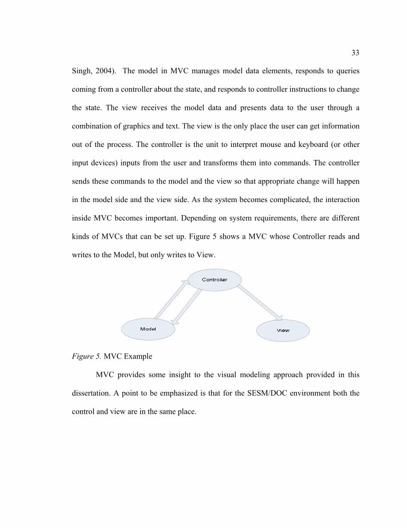
33
Singh, 2004). The model in MVC manages model data elements, responds to queries
coming from a controller about the state, and responds to controller instructions to change
the state. The view receives the model data and presents data to the user through a
combination of graphics and text. The view is the only place the user can get information
out of the process. The controller is the unit to interpret mouse and keyboard (or other
input devices) inputs from the user and transforms them into commands. The controller
sends these commands to the model and the view so that appropriate change will happen
in the model side and the view side. As the system becomes complicated, the interaction
inside MVC becomes important. Depending on system requirements, there are different
kinds of MVCs that can be set up. Figure 5 shows a MVC whose Controller reads and
writes to the Model, but only writes to View.
Figure 5. MVC Example
MVC provides some insight to the visual modeling approach provided in this
dissertation. A point to be emphasized is that for the SESM/DOC environment both the
control and view are in the same place.

34
2.4 Model-Driven Engineering
There is always a gap between the field of system design and the field of
modeling and simulation. On one hand, system designers have the domain knowledge of
the system but they may not have the training for writing the simulation model code to
run the simulation. On the other hand, modeling and simulation people have the skills to
write the simulation model code, but they don’t know how to set up the logical model and
how to make verification and validation according to particular domain knowledge. The
consequence is that either the system designer spends too much time learning to write the
simulation code (which may not properly reflect the logical model), or the system
designer spends too much time communicating with the simulation people to make sure
the simulation people understand the rationale inside the model. The result of this kind of
communication always leads to unsatisfactory simulation code due to the lack of domain
knowledge background on the part of the simulation people. In reality, even within the
people who have the domain knowledge, their levels of capability to handle the problem
related to domain knowledge are different. It is commonly accepted within industry, such
as the network industry, that fewer than 10% of engineers working in the field have
sufficient knowledge and experience to tackle the complexity in the design phases; that is
to say, only this group of people can process the knowledge and overview of the elusive
system architecture that allows them to identify the details in network nodes, network
services, protocols, and messages that will be affected by changing network
functionalities. The other 90% of engineers are capable of performing the execution

35
phase which means they can only operate the system (Muth, 2005). This generalization
serves as one of the motivations behind the attempts to automate the generation of the
code for proprietary programming language, which later gradually becomes a reality for
standardized language.
Another major challenge regarding system design in modeling and simulation is
how to transform models among different platforms. In recent years, some popular
middleware platforms such as J2EE (SUN, 2005), .NET(Microsoft, 2006) and
CORBA(Object Management Group, 2005) have grown rapidly. These platforms contain
thousands of classes and methods with many intricate dependencies and subtle side
effects. Designers have to expend extra effort manually porting application code to
different platforms. This process is time consuming and error prone.
Model-driven engineering (MDE) is the bridge between the domain knowledge
and the modeling and simulation. Several MDE methodologies are provided to try to
solve the above problems by integrating the process of design and lower level
implementation. Computer-Aided Software Engineering (CASE), Model-Integrated
Computing (MIC), and Model-Driven Architecture (MDA) are the three major ones
among the MDE methodologies.
Computer-Aided Software Engineering (CASE) began in the 1980s. It provides
general purpose graphical programming representations such as state machines, structure
diagrams, and dataflow diagrams to the designer in order to describe their thoughts for
the system (Schmidt, 2006). This helps designers to avoid detailed language
implementation. However, CASE has some fatal problems. One is that there is still a gap

36
between the designer and the people who do the detail implementation. The programmers
have to read the graphical representations to understand the design before they start to do
the modeling and simulation. It is very easy for a misunderstanding to occur in this
process. The other problem is the implementation code is not generated automatically,
which means people still need to manually code. This is tedious and time consuming.
Those problems make CASE have relatively little impact on commercial system
development. EDEN (Erdogan, McFarr, & Maglidt, 1989) and AVAT (Dai & Scott,
1995) are examples of CASE. Therefore, the current most popular MDE methodologies
are MIC and MDA.
2.4.1 Model-Integrated Computing (MIC)
Model-Integrated Computing (MIC) has been developed over a decade at the
Institute for Software Integrated System (ISIS), Vanderbilt University. This approach
extends the usage scope of models so that they can form the “backbone” of the model-
and-simulation integration process. The key elements in MIC are (Schmidt, 2006):
Domain-Specific modeling language (DSML) – DSML is a kind of language
whose type systems formalize the structure, behavior, and constraints of particular
application domains, such as the computer network systems, the supply chain networks,
and online financial services. It uses meta-models which is the basic unit model defining
the relationships among concepts within a domain and precisely specifies the semantics
and constraints associated with these domain concepts. Using DSML, designers can
express design intent declaratively rather than imperatively. For example, when a

37
designer wants to design an antivirus system, what he needs to do is just declare what
kind of processor (single thread or multiple threads) should be in the system; he has no
need to code the command line by line to implement it.
Transformation engine and generators – Transformation engine and generators
can analyze certain aspects of models and then synthesize other type of artifacts such as
the simulation model source code, and XML description. The source code generated can
be run in a simulator. The transformation engine and generator can also help designers
check to determine if the models specified in DSML are correct according to the domain
constraints by running the simulation code. The life cycle of MIC (Gokhale, Batarajan,
Schmidt, & Wang, 2002) is illustrated in Figure 6.
Figure 6. Model-Integrated Computing Life Cycle
Model-Integrated Computing helps the system designer avoid the trouble of the
implementation of their models. A well-defined DSML can automatically generate the
simulation code. With MIC, system designers can shift their focus of modeling and
simulation from implementation technology domain towards the concepts and semantics
in the problem domain. The debugging and the model checking can be done in the

38
modeling level but not the detailed code level. Even for the people who are familiar with
implementation of the simulation model, the MDE reduces costs and shortens the time to
market. Automatic generation of code is always faster than manual generation. Examples
of MIC are CoSMIC and ECSL (Krishnakumar, Gokhale, & Karsai, 2006).
However, there are still some drawbacks to MIC in practice. First, the application
of a particular DSML is very limited because it is only for one domain. Second, the
designer has to learn how to use the DSML to describe logical models. DSML is much
easier than a general purpose language like C++. However, if designers need to do design
for several domains then they have to be familiar with a different DSML and the learning
curve becomes bigger.
2.4.2 Model-Driven Architecture (MDA)
Model-Driven Architecture (MDA) was defined and trademarked by the Object
Management Group (OMG) in 2002. Unlike MIC, MDA presents systems using OMG’s
general-purpose Unified Modeling Language (UML) (and its according profile, which is
the extensions of UML) and transforms these models into artifacts which can run on
different platforms such as EJB, .NET, and the CORBA Component Model (CCM).
Using MDA, the system designers can use the UML present logical model. This
makes the logical models have unified syntax and can be shared between designers
easily. A UML presented logical model is known as Platform Independent Model (PIM).
UML is a malleable language and provides a build-in extension mechanism. Adding with
build-ins, UML can support middleware-specific modeling. This extension of UML is

39
called UML profiles (Frankel, 2003). UML profiles can help transform a Platform
Independent Model (PIM) to a Platform Specific Model (PSM). The further step is to
transform PSM to a source code which can run in the particular platform. The procedure
in MDA is shown in Figure 7.
Figure 7. Model-Driven Architecture Procedure
In MDA, designers use their expertise to develop PIM. They do not need to worry
about the platform issues and coding details – this highly improves the productivity. The
UML in MDA helps to standardize the logical model. The same PIM can be
automatically transformed into a variable PSM for different purposes. This makes the
design more portable. The MDA framework raises the level of abstraction of the system
design. IBM Rational Rose XDE is a MDA example which combines a modeling
environment with a code-oriented tool set to create solutions in a variety of architectural
styles (Brown, 2004). Another MDA example is MODEST (Model-Driven Enterprise
System Transformer), which was developed by Chronos Software, Inc (Rutherford &
Wolf, 2003).
MDA makes a big step for the integration of design and implementation.
However, there are still major drawbacks in MDA. First, as the language to define a PIM,
UML has some limitations. UML is designed along with the object-oriented concepts. So

40
to define a non-object-oriented model, designers need to create a new meta-model, which
is error prone and time consuming. UML shows its strength as a unified language but as
the side effect it looses the particularity in a particular domain. Using UML to present a
set of domain knowledge is not easy. In order to generate the executable code, MDA
needs two steps of transformation: transformation from PIM to PSM and transformation
from PSM to code. This means that MDA can only provide a code template which needs
extra work (manually) to add some behavior functions to run. Used in the modeling and
simulation field, MDA cannot realize the real model-and-simulate paradigm.
2.4.3 Model Design Methods and Tools
The model design plays an important role in model driven engineering. The
model design for a system is not trivial. The model designer needs the knowledge of
system engineering, software engineering, and the system domain knowledge, etc. There
are methodologies and tools to help people to specify and design the model. In this
section we will introduce some of them.
Entity Relationship (ER) Modeling: Entity Relationship Modeling is a type of
conceptual data model which is used in relational database design (Chen, 1976). The
graphic view of ER model is ER diagram, which represents the conceptual database as
viewed by the end user. The ER model has three main components: entities, attributes,
and relationships. An entity refers to a table or an object in the database. Attributes are
particular properties that describe the entity. Each entity has at lease one attribute. A
relationship refers to an association between entities. ER modeling translates different

41
views of data among database designers, programmers, and database users. The ER
diagram defines data processing and constraint requirements in order to help meet the
different views and implement the database. Through the ER diagram, the data model
entities, the attributes these entities contain, and the relationships among these entities are
clearly presented.
System Entity Structure (SES): System Entity Structure is a structural knowledge
representation that systematically organizes a family of possible structures of a system
(Zeigler, Praehofer, & Kim, 2000). This kind of family includes system entities as well as
the decomposition and coupling relationships. In SES, an entity is a model of a real world
object. The decomposition is the process of how an entity can be broken into sub-entities.
These sub-entities may be decomposed further. The coupling relationship specifies how
sub-entities in an entity can relate together and reconstitute the entity. SES is based on
system theory and gives the hierarchical decomposition structure of a system. SES aids in
the design and analysis of a complex system by breaking it down into finite small and
easy subsystems.
Extensible Markup Language (XML): Another data modeling language is XML.
XML is a general-purpose markup language. Its primary purpose is to facilitate the
sharing of data across different information systems, particularly via the Internet. XML
allows a user to define a model in a markup language and share the model information in
different platforms.
XML is a simplified subset of the Standard Generalized Markup Language
(SGML) and is designed to be relatively human-legible. By adding semantic constraints,

42
application languages can be implemented in XML. These include XHTML, RSS,
Scalable Vector Graphics, and thousands of others. Moreover, XML is sometimes used as
the specification language for such application languages. XML is recommended by the
World Wide Web Consortium (W3C). It is a fee-free open standard. The W3C
recommendation specifies both the lexical grammar and the requirements for parsing.
(World Wide Web Consortium, 1998)
Unified Modeling Language (UML): The Unified Modeling Language is a
standardized specification language for object modeling in the field of software
engineering (World Wide Web Consortium, 1998). UML is officially defined at the
Object Management Group (OMG) by the UML metamodel, a Meta-Object Facility
(MOF) metamodel. It is a general-purpose modeling language that includes a graphical
notation used to create an abstract model of a system, referred to as a UML model. UML
was designed to specify, visualize, construct, and document software-intensive systems.
UML has been a catalyst for the evolution of model-driven technologies, which include
Model Driven Development (MDD), Model Driven Engineering (MDE), and Model
Driven Architecture (MDA). By establishing an industry consensus on a graphic notation
to represent common concepts like classes, components, generalization, aggregation, and
behaviors, UML has allowed software developers to concentrate more on design and
architecture.
UML is not restricted to modeling software. It is also used for data modeling,
business process modeling, systems engineering modeling, and representing
organizational structures. UML is extensible, offering both profiles and stereotype
43
mechanisms for customization. The semantics of extension by profiles has been improved
with the UML 2.0 major revision. The current version of UML (early 2007) is Version
2.1.1.
Systems Modeling Language (SysML): Systems Modeling Language is a domain
specific modeling language for system engineering. It supports the specification, analysis,
design, verification and validation of systems. SysML has improvements over UML such
as: having more flexible and expressive symatics, easier to being learned and applied, and
supporting common kinds of table allocations. SysmML reduces UML's size and
software bias while extending its semantics to model requirements and parametric
constraints. (Hause, Thom, & Moore, 2005)
Scalable Entity Structure Modeler (SESM): Scalable Entity Structure Modeler
(Fu, 2002) is a framework aimed at hierarchical component-based modeling. Its
specification capabilities are derived from ER, System Entity Structure (SES), and
Object-Oriented (OO) modeling approaches. It introduces visual modeling and the
transformation of logical models into simulation models. In its realization, SESM is a
modeling engine for developing specifications that have formal logical syntax and
semantics as well as visual and persistent representations. The simulation model can be
partially generated based on the models which are stored in the database.
Many modeling and simulation software products are used in academia and
industry. Some popular generic system modeling and simulation tools are MATLAB
(Higham & Higham, 2000), Simulink (Karris, 2006), DEVSJAVA (Arizona Center for
Integrative Modeling and Simulation, 2007) and PowerDEVS (Kofman, Lapadula, &
44
Pagliero, 2003). The work in this dissertation provides co-design modeling methods to
support distributed network modeling and focus more on network modeling and
simulation. There are a variety of simulation environments that support the modeling of
computer networks such as NS-2 (Information Sciences Institute, 2004), GloMoSim
(Global Mobile Information Systems Simulation Library, 2005), OPNET (OPNET
Technologies, 2004), QualNet (Jaikaeo & Shen, 2005; OPNET Technologies, 2004),
TOSSIM (Levis, Lee, Welsh, & Culler, 2003), etc.
NS-2: NS-2 is a discrete event simulator for networking research. It provides
support for simulation of Transmission Control Protocol (TCP), routing, and multicast
protocols over wired and wireless networks. (Information Sciences Institute, 2004)
In the application layer, NS-2 provides two basic types of applications: traffic
generators and simulated applications. There are currently two “simulate application”
classes derived from NS-2 Application class: Application/ File Transfer Protocol (FTP)
and Application/Telnet. These classes work by advancing the count of packets available
to be sent by a TCP transport agent. The actual transmission of available packets is still
controlled by TCP’s flow and congestion control algorithm. In NS-2, all of the
applications are limited to implementations of low level computer networks with the
TCP/UDP constrains. NS-2 supports simulation applications for detailed computer
networks in the lower level.
In the transport layer, with the support of transport layer agents, NS-2 provides a
strong support for the transport protocol simulation. The network level packet header
field helps the routing in the NS-2 network layer.

45
The NS-2 link layer can potentially have many functionalities, such as queuing
and link-level retransmission. The need of to have a wide variety of link-level schemes
leads to the division of functionality into two components: Queue and LL (link-layer).
The Queue object, simulating the interface queue, belongs to a Queue class in NS-2. The
LL object implements a particular data link protocol, such as Automatic Repeat Request
(ARQ). By combining both the sending and receiving functionalities into one module, the
LL object can also support other mechanisms such as piggybacking.
At the bottom of the NS-2 protocol stack, the physical layer is composed of two
simulation objects: the Channel and Classifier/Mac. The Channel object simulates the
shared medium and supports the medium access mechanisms of the MAC objects on the
sending side of the transmission. On the receiving side, the Classifier/Mac is responsible
for delivering and optionally replicating packets to the receiving MAC objects.(Chung &
Claypool, 2005; Fall & Kannan, 2005).
NS-2 has strong support for the layers under the application layer. However, in
the application layer, NS-2 only provides limited facilities for the user to define
customized services. In NS-2, the node module is the main part that supports the
applications. A node is composed of three parts: address classifier, Port classifier and
agents. The address classifier is used to support unicast (although NS-2 also supports
multicast, by default, the node is unicast) packet forwarding. The address classifier
contains a slot table for forwarding packets to foreign nodes. All packets not destined for
this node (and hence forwarded to the port classifier) are sent to the default target, which
points to an agent. In NS-2, an agent supports packet generation and reception.

46
This kind node structure does not provide the management of the work processed
in the node so it is hard for the modeler to model and simulate what is going on inside the
node when the system is running. It is also hard to present the dynamic behavior of the
node unless the extra code is added by the modeler which means the modeling of
software is ad hoc and not supported with well-defined specification. Furthermore, there
is a strong dependency among some of the NS modules. As a result, it can be challenging
to model new protocols or to make changes to existing protocol models. Given its
complexity and low-level detailed models, it is necessary to have the knowledge of NS-2
at the software implementation and design level for serious simulation. NS-2 supports the
fine grain modeling of protocols rather than the quantum level modeling (Information
Sciences Institute, 2004). NS-2 is not intended for disciplined integration of hardware and
software simulation modeling. It supports simulating software communication protocols
for network devices instead of simulating a set of software applications distributed across
processors and network devices.
From a usability aspect, NS-2, which is a Unix-based environment, does not offer
a user friendly simulation environment. All of the simulation results are stored in data
files (simulation logs). The stepping and control is hard to implement. NS-2 is based on
C, which does not provide a purely object-oriented way to set up a model hierarchy.
Consequently, the use of NS-2 can require additional time and effort for developing
models that are not already available.
GloMoSim: GloMoSim is a library-based sequential and parallel simulator. It is
designed as a set of library modules, each of which simulates a specific communication

47
protocol in the protocol stack. GloMoSim supports its application layer service for
wireless network systems. Users can get the low level statistics In the GloMoSim
application layer such as the total number of packets sent and the total number of packets
dropped. GloMoSim supports wireless FTP and telnet application. The statistics that can
be obtained are the start/end time, bytes sent/received and throughput. For the transport
layer in GloMoSim, there are various protocols which can be used individually or
concurrently. Protocols such as IP with Ad hoc On Demand Distance Vector (AODV),
Bellman-Ford, Dynamic Source Routing (DSR), and Fisheye, are supported in the
GloMoSim network layer, and Carrier Sense Multiple Access (CSMA), IEEE 802.11 and
Multiple Access with Collision Avoidance (MACA) are supported in the link layer. In the
physical layer, GloMoSim’s models are implemented based on the DSSS PHY reference
configuration in the IEEE 802.11 standard (Gerla, Zhang, Tang, & Wang, 1999; Global
Mobile Information Systems Simulation Library, 2005; Pei, 1997).
The library in GloMoSim is written in PARSEC, a C-based parallel simulation
language. Users have to hard code their own protocols or models if they are not found in
the library. Only limited network service models are provided, especially in the
application layer.
OPNET: OPNET is a commercial network simulator which was first introduced
in 1986. It provides a comprehensive development environment supporting the modeling
of communication networks and distributed systems. OPNET has a very user friendly
GUI to help the user to build its models (OPNET Technologies, 2004).

48
In the application layer, the Application Characterization Environment (ACE) in
OPNET directly addresses the end-to-end application performance analysis issues. This
ACE environment focuses on the application performance monitor instead of providing a
flexible mechanism for users to model different user-defined applications in the lower
levels. Another package in OPNET, the ACE Decode Module (ADM) provides some pre-
defined application model and protocols but to modify and customize them in lower
levels is a challenge. OPNET also supports the transport layer and can be used to study
the impact of TCP and UDP. The analysis data in the transport layer includes data
volume sent and received, connection establish/abort counts, and UDP end-to-end latency
(Highland System Inc., 2005). OPNET shows its strength in the network layer. Many
detailed studies can be made in this layer with OPNET such as different routing
protocols. In the link layer, OPNET can be used for both wired networks and wireless
networks (Chan, 2005; Zhong, Rabaey, Guo, & Shah, 2001). In the physical layer,
OPNET is used to analyze the throughput and received power (Highland System Inc.,
2005). The downside is that OPNET has limited scalability. Currently, it only can
perform well with no more than hundreds of nodes in the network.
QualNET: QualNet is a high speed network modeling tool used to simulate a wide
range of computer networks. It is a commercial derivative of GloMoSim. Its simulation
kernel runs a large library of detailed protocol models. In the application layer, QualNet
generates traffic based on network protocols such as ftp, and telnet. Users can choose the
application layer protocols from the GUI which is connected to the model library. The
transport layer in QualNet is in charge of TCP and UDP protocols. QualNet currently
49
only provides routing protocols in its network layer. The link layer manages the packets
store and forward with multiple access control protocols for IEEE 802.11, and 802.3. The
physical layer provides a noise model and parameters specific to 802.11b, it also has a
omnidirectional antenna model for wireless network (Jaikaeo & Shen, 2005). QualNet
shows its strength in large-scale network simulation. However, as was the case in
GloMoSim, models which can not be found in the library are hard to add for the
simulation.
TOSSIM: TOSSIM is a simulator for embedded systems in sensor networks. Its
primary goal is to provide a high fidelity simulation of TinyOS applications. For this
reason, TOSSIM focuses on simulating the open source TinyOS and its execution. So the
applications that run in TOSSIM are the applications that belong to TinyOS. Also,
TOSSIM simulates the network at the bit level. Currently, TOSSIM simulates the 40Kbit
RFM mica networking stack, including the MAC, encoding, timing, and synchronous
acknowledgements (Levis & Lee, 2003; Levis, Lee, Welsh, & Culler, 2003).
In the real world, numerous systems can be studied as network systems, such as
computer networks, supply chain networks, work-follow management, and transportation
systems. These are all constructed from two building blocks: nodes and links. The node is
a processing/computing unit, and the link is the transportation media. The above
simulation environments show their strength for modeling and simulating the link— the
transportation media part of the system. However, they do not provide enough facilities
for modeling and simulating the nodes— the processing/computing unit. There are two
reasons for this. First, all of these simulation environments are not intended for

50
disciplined integration of hardware and software simulation modeling. They do not
separate the implementation of hardware and software. The detailed study of the services
in the nodes requires the separation of the models for hardware (resources) and software
(services). The second reason is that all of the simulation environments are designed for
the study of the computer network protocols. The nodes (or application layer) in these
protocols only provide the traffic generation based on basic network protocols such as
FTP, and telnet. This limits the usage of these simulation environments only for computer
network transportation protocols.
Most of the simulation environments above do not provide a purely inheritance
hierarchy relationship for the models. In the above simulation environments, only
OPNET provides a formal object-oriented view for models. Some of the simulation
environments provide users friendly GUIs such as GloMoSim, OPNET, QualNet, others,
such as NS-2, do not. Some of them are good for large-scale simulations, such as
QualNet, while some are not, such as OPNET.
DEVS/DOC: The DEVS/DOC approach extends the generic DEVS modeling
concepts and models to support co-design specification of network systems. This co-
design approach enables modelers, for example, to model a computer network in terms of
separate sets of hardware and software components and software to hardware mappings.
With this approach, the hardware and software layers can be independently specified and
the software to hardware mapping can be used to configure alternative system designs.
The flexibility is important for evaluating alternative hardware topologies (e.g.,
computing resources offered by individual nodes and their combination) given software

51
functionality and quality attributes (e.g., desirable quality of service afforded by
individual software components and their combination) (Hild, Sarjoughian, & Zeigler,
2002).
2.5 Summary
This chapter describes the background and related work for modeling and
simulation in the context of system analysis and design. Related concepts in system
engineering, system theory, and modeling simulation are reviewed. A survey of the
related modeling and simulation frameworks and approaches are given in this chapter to
illustrate their strengths and limitations. Compared to the work in this dissertation, these
modeling approaches in the survey do not have clear boundaries to systematically define
the software and hardware in a network system from the visual and persistent modeling
point of view. They do not provide the descriptions of the relationship between the
software and hardware model visually. In a word, they fall short of specifying the
separation and synthesis of software and hardware components in a co-design network
system through visual and persistent modeling.

3 MODELING AND SIMULATION APPROACHES AND TOOLS
In the previous chapters, we briefly introduced SESM, DEVS, and DEVS/DOC.
These are the basic elements for the co-design modeling approach developed in this
dissertation. Each will be introduced in detail as appropriate.
3.1 Scalable Entity Structure Modeler Concepts and Approach
Scalable Entity Structure Modeler is a modeling methodology for component-
based modeling of large-scale and complex systems (Fu, 2002; Sarjoughian, 2001).
SESM provides modeling of a system using three complementary model types: Template
Model (TM), Instance Template Model (ITM), and Instance Model (IM). A Template
Model is defined as either a primitive or a composite component with input and output
ports and port values. A primitive template model specification contains state variables
and a name. The primitive model is the basic model unit in SESM and cannot be
decomposed. A composite model has one or more primitive models or other composite
models. The relationship between two connected model (primitive or composite model)
ports is called a link (Sarjoughian, Fu, Bendre, & Flasher, 2007). A composite template
model specification has links, a name, and it can be defined to have a hierarchy of length
of two. The composite model can be decomposed into other composite models or
primitive models. This primitive-composite modeling structure allows the system
designer to decompose the large-scale complex system and deploy the component models.
The difference between an instance template model and a template model is that
an instance template model can have a finite hierarchy with a length greater than two.
The instance template models introducing multiple-levels of hierarchy using
53
decomposition and specification. An instance model is an instantiation of an instance
template model where the multiplicity of instances of a model is specified. Usually, a
designer creates the template models, instance template models, and instance models in a
sequential manner. In the instance model generation stage, the decision of which
specified model component to use is made.
The primitive-composite model structure provides the system designer the facility
to decompose a large-scale complex system into a finite number of simple systems. The
relationship between the three model types gives the system designer the ability to
specify different resolutions of the system model. This decomposition helps the system
designer create alternative models according to its desired resolution, which are important
in the modeling of large heterogeneous systems.
SESM aims to help designers with system design by creating and verifying
models for scalable systems such as a network system. SESM captures three sets of
system model properties: structure, structural complexity and behavior. Model structure
includes the model’s name, input and output ports, the coupling relationship between
multiple models, and the composition relationship between multiple models. Structural
complexity captures the model’s structure scale, such as the number of parts. Complexity
is important for large-scale systems and hierarchical system models (Bendre &
Sarjoughian, 2005; Mohan, 2003; Sarjoughian, 2005). Model behavior includes model
input and output value types, and state variables (Bendre, 2004; Bendre & Sarjoughian,
2005).

54
The goal of the SESM model engine is to handle the modeling of a family of
modular, hierarchical models at different levels of abstraction. The support from a
database is important for this kind of large-scale modeling in terms of persistence, the
persistent model data management, and model transformation. SESM saves the logical
models as persistent models using the schemas shown in Figure 8 (Bendre, 2004; Fu,
2002; Mohan, 2003; Sarjoughian, 2005).
Figure 8. Basic SESM ER Diagram
3.1.1 Framework and Related Modeling and Simulation Architecture
SESM, as a modeling framework, has the following architecture shown in Figure
9. The SESM client includes the user interface through which designers can design and
view models. The SESM server stores the models into a database. Clients can read the
model data from the database and its “write” requests can be passed through the server to
TemplateModel
componentOf
ITMtoIM
TMItoSIM
InstanceModel componentOfI
0,1
1,11,N
0,N
1,1
0,N
0,1
0,N
0,1
InstanceTM
0,N
TMtoITM InstanceTM

55
the database. The server can both “write” and “read” to the database. Figure 9 shows the
data flow in the SESM architecture.
Figure 9. SESM Architecture
In the SESM environment, system designers input the information and constraints
of the desired models. In Figure 9, the model engine captures the properties of logical
models according to the designers’ commands and stores the logical models as the
persistent model in the relational database. Designers can then view the corresponding
visual model. In the SESM server, there is a translator which translates the system-
theoretic model specification to XML or DEVSJAVA.
The translator can generate the partial simulation model, which after some
extension to capture the behavior property, can run in a simulation environment.
Currently, the SESM environment can generate a simulation code in DEVSJAVA. The
primitive model in SESM is transformed into a DEVSJAVA atomic model and the
composite model in SESM is transformed into a DEVSJAVA coupled model. The atomic
model is partially generated and the coupled model is completely generated (in the sense
to present the coupling relationship). DEVSJAVA models can be completed and
simulated using the DEVSJAVA simulation engine as shown in Figure 10. By analyzing

56
the simulation results coming from DEVSJAVA, the designer gains a much better
understanding about which design solution is the desired one based on the results of the
simulation models. The whole process discussed above is very important to designers for
decision making. It helps them choose the better alternative model for the system.
The logical model is designed as the visual model, and saved in database as the
persistent model. With the translator, the logical model can be transformed into the
simulation model which runs in the simulation engine. The modeling transformations in
SESM are shown in Figure 10.
Figure 10. Modeling and Simulation with SESM
3.1.2 Model Example
A simplified AntiVirus system is illustrated here in SESM to show how SESM
can be used to design models. An Anti-Virus system is intended to protect a network of
computers from potential virus attacks. The primary objective of this system is to keep
the computers on the network secured and virus-free. A simplified model of an AntiVirus
system consists of a detectUnit and a killUnit. The detectUnit aims to find a virus and

57
sends it to the killUnit. The killUnit then kills the virus and sends the clean file out. If
there is no virus, the detectUnit will send the file out.
The following is the detectUnit logical model example using the DEVS
specifications:
Inports = {in, alertSignal}
Outports = {out, outVirus}
States = {idle, busy}
External transaction function: receive files and detect virus;
Internal transaction function: change state;
Output function: send out virus or clean files.
The user of SESM first designs the logical model of the primitive model:
detectUnit and killUnit, as shown in Figure 11.
Figure 11. Visual Model of detectUnit and killUnit
With these two primitive models, a composite AntiVirusSystem can be built in
SESM, as shown in Figure 12. The input/output variables can be added into the model
input/output ports. SESM also supports non-simulatable models which are models can be
defined in DEVSJAVA but cannot be simulated. An example is the model containers.
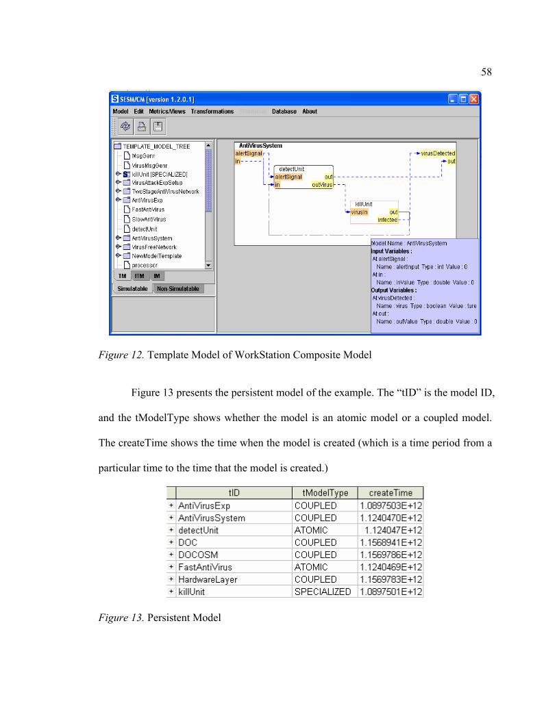
58
Figure 12. Template Model of WorkStation Composite Model
Figure 13 presents the persistent model of the example. The “tID” is the model ID,
and the tModelType shows whether the model is an atomic model or a coupled model.
The createTime shows the time when the model is created (which is a time period from a
particular time to the time that the model is created.)
Figure 13. Persistent Model

59
Given the persistent model support, SESM also provides structural complexity
metrics for the system model. A simple example for the WorkStation in the AntiVirus
system is shown in Table 5. The value in the metrics gives the name and type of the
model and the number of model attributes.
Table 5
SESM Structural complexity Metrics
Attribute Value
Model Name AntiVirusSystem Model Type Composite Children Immediate 2 Total 2 Ports Input 2 Output 2 Total 4 Couplings Internal 2 External input 2 External output 2 Total 6
With the structural complexity metrics, we can obtain information such as how
many primitive models the system has, how many composite models the system has, and
how many couplings the system has. Through the translator, the modeler can have the
XML specification of the model and DEVSJAVA source code template of the model, as
shown in Table 6.

60
Table 6
XML and DEVSJAVA Code Generated In SESM
XML detectUnit Model
<model> <atomicModel name="detectUnit"> <inport name="alertSignal"> <inportVariable name="alertSignal"> <inportVariableType name="entity"> <inportVariableValue>alertInput</inportVariableValue> </inportVariableType> </inportVariable> </inport> </inport> <outport name="out"> <outportVariable name="out">
…….
DEVSJAVA detectUnit Model
public class detectUnit extends ViewableAtomic{ public Processor(){ this("detectUnit", 0.0); } public detectUnit (String name, processing_time){
super(name); this.processing_time = processing_time; addInport("alertSignal"); addInport("in");
…......
SESM can be used to design models but it does not distinguish between the
software model and hardware model in a system. It is difficult for the modeler to design a
software model and a hardware model separately. The lack of separation of software
models and hardware models puts limitations on the application of SESM in co-design
system modeling. For example, in the previous AntiVirus system, the detectUnit created
in SESM does not tell people whether it is software (a software application for detecting

61
viruses like the Norton antivirus system) or hardware (an antivirus firewall). This brings
problems when modelers add state variables or input/output ports into the model. For
example, if the detectUnit is a software model, then how much memory the software
requires should be added as a state variable. However, if it is a hardware model (the
firewall) then the processing speed and bandwidth should be a concern. In co-design
system modeling, it is important to extend SESM to systematically model the software
and the hardware.
3.2 Discrete Event System Specification
Discrete Event System Specification (DEVS) is the specification for presenting
the structural and behavioral property of discrete event systems. With the popularity of
applications of computers in system engineering, discrete event modeling becomes an
attractive formalism due to its relationship with digital computing (Sarjoughian & Cellier,
2001; Zeigler, Praehofer, & Kim, 2000).
3.2.1 Concepts and Approach
DEVS classifies models as one of the two types: the atomic model and the
coupled model. The atomic model presents the basic level of DEVS formalism with
specifications of the basic components of the system. The coupled model, which is
composed by at least one atomic model and coupling relationship among these models,
realizes the compositional constructs for structuring DEVS models into system structure
hierarchies. Both atomic and coupled models can be simulated using sequential
computation or various forms of parallelism. In a DEVS atomic model, there are five

62
methods (external transaction function, internal transaction function, confluent function,
output function, and the time advanced function) which handle the state changes within
the atomic model. The DEVS coupled model designates how (less complicated) models
can be coupled together and how they interact with each other. The specificaiton of
DEVS is in following structure:
M = <X, S, Y, δint, δext, δcon, λ, ta>
Where
X is the set of input values
S is a set of states
Y is the set of output values
δint: S→S is the internal transition function
δext: Q*Xb→S is the external transition function, where
Q = {(s, e)|s∈S, 0 ≤ e ≤ ta(s)} is the total state set
e is the time elapsed since last transition
δcon: Q*Xb→S is the confluent transition function
λ: S→Y is the output function
ta: S→R+0, ∞ is the time advance function
As the basic model unit, the atomic DEVS model defines the states and the
associated time bases. The DEVS coupled model designates how systems can be coupled
together. A typical model in DEVSJAVA has two sets of input/output ports: input ports
and output ports. Briefly, the external transition function dictates the model’s new state

63
when an external event occurs (input coming from the input ports). The internal transition
function dictates the system’s new state when no event occurred since the last transition.
The output function generates output through output ports and the confluent transition
function decides the next state in case of collision between external and internal events.
The time advanced function tells how long the model would stay in the current state if
left without interruption.
3.2.2 DEVSJAVA Simulation Environment
Many implementations of the DEVS framework have been developed in popular
programming languages including Java. DEVSJAVA is a Java implementation of DEVS
specification. The DEVSJAVA 2.7 and 3.0 environments (in this dissertation the
DEVSJAVA 3.0 will be used) are new generations of DEVS-based modeling and
simulation environments that separate the modeling and simulation engines and the user
interface. These environments offer new capabilities not found in DEVSJAVA 2.63,
such as model type discovery and run-time execution using a logical clock or a wall clock
(Cho, Zeigler, Cho, & Sarjoughian, 2000). DEVSJAVA 2.7 and 3.0 offer strong
separation between modeling and simulation engines. This is important for supporting
distributed simulation using alternative technologies such as CORBA (Object
Management Group, 2005) and HLA (Institute of Electrical and Electronics Engineers,
2000). One of the key DEVSJAVA Application Programming Interfaces (APIs) is GenCol
which provides the collections for models (Park, Zeigler, & Sarjoughian, 2001) . Table 7
shows the important modules in DEVSJAVA and each of their purposes.

64
Table 7
DEVSJAVA 3.0 Modules
Module Purpose GenCol non-simulation structure modeling genDevs.modeling atomic and coupled model specification genDevs.simulation abstract atomic and coupled simulator specification simView simulation visualization
DEVSJAVA 3.0 provides the API which contains the base class entity, that serves
as the root class for the modeling (genDevs.modeling), simulation (genDevs.simulation), and
visualization (simView) modules (Park, Zeigler, & Sarjoughian, 2001). This module
provides more collection facilities than the Java Development Kit (JDK) 5.0 collection
API. GenCol has its own container classes using the entity class from the Container library
from DEVSJAVA 2.6.3, as shown in Figure 14. Figure 15 presents the classes in GenCol
and their relationships. The combination of Java Collection API and GenCol APIs,
therefore, offer all of the functionality that was in Container API used in DEVSJAVA
2.6.3 as well as others needed for the new modeling and simulation packages in
DEVSJAVA 3.0. DEVSJAVA 3.0 also provides interfaces for designing alternative
models with different behaviors.

65
entitycontainer
bagorder message
set
relation
function
list
Figure 14. DEVSJAVA 2.63 Container Specification
GenCol
ZFunction
ZFunction Interface
Function
Function Interface
JDK 5.0
Hashtable
BagPair
ensembleBagname : Stringh : Hashtablesize : Integer
getTheClass()printClassMethods().................()tellAll()
relation
Relation Interface
ZRelation
ZRelation Interface
entity
Entity Interface
Object
Figure 15. GenCol Container Specification
In DEVSJAVA 3.0, the modeling module provides basic modeling elements
including atomic and coupled models such as the base class devs. The devs class extends
class entity with methods to add input and output ports so that a model can send and
receive messages. Extending from devs, the atomic class provides state assignment and
functions to process external and internal events. With DEVSJAVA 3.0, all atomic
models can run as a separate component with the viewableAtomic and all coupled models

66
can be executed as a separate system with viewableDigraph (as shown in Figure 16). The
other basic modeling elements in the modeling module are ports and coupled, which allow
coupling of atomic and coupled models.
devsdigraph atomic viewableAtomicviewableDigraph
Object
Enti tyInterface
entity
Figure 16. viewableAtomic and viewableDigraph
Similar to the modeling module, the simulation module contains classes that
execute the atomic and coupled models which includes the transmission of messages. The
classes in the simulation package are realizations of the DEVS parallel abstract simulator
(Arizona Center for Integrative Modeling and Simulation, 2007). The atomicSimulator and
coupledSimulator are two of the key classes for handling the timing of atomic and coupled
models and their exchange of output and input events. The simulator design is shown in
Figure 17.
atomicSimulationInterface
atomicSimulator
coreSimulatorInterface
coordinator
coordinatorInterface
coupledCoordinator
coupledCoordinatorInterface
Figure 17. Simulator Utilities
Figure 18 shows another aspect which cannot be found in DEVSJAVA 2.63, the
visualization module. The module is supported by the SimView package, which provides
services for visualizing the simulation of the atomic and coupled models (viewableAtomic

67
and viewableCoupled), configuring simulation models, and executing and viewing the
simulation dynamics.
Figure 18. Graphical View of An Atomic Model in DEVSJAVA 3.0
As an example, an atomic LCN model called hub is depicted in DEVSJAVA in
Figure 18. This DEVSJAVA Simulation Viewer generated by SimView has two
functionalities: model display and simulation control. As shown in Figure 18, a user uses
the “configure” button to choose the model packages. “DOC” and “hub” at the top of
Figure 18 shows that the “hub” model in “DOC” package is chosen for display. In the
middle part of the simulation viewer is the display of the chosen model. A model
component can receive input messages on one or all of its input ports (e.g., inLink1) and
concurrently produce output messages on its output ports (e.g., outLink2). The states of the
hub atomic model (e.g., execution phase (passive) and the duration in which the hub stays
in phase passive (∞)) can be viewed at run time. The execution speed of the hub can be
controlled via the “real time factor”. The “step”, “run” and “restart” buttons in the bottom
of the simulation viewer are for the simulation control purposes. The “step” button can
show the single simulation step based upon a single simulation event.

68
3.2.3 Simulation Model Example
The AntiVirus system in Section 3.1.2 is illustrated here for the DEVSJAVA
framework. The AntiVirus system is an anti-virus network system including a
“detectUnit” model to detect virus messages passing into it, and a “killUnit” model which
can get rid of the virus messages. These two models compose a coupled model, the
“AntiVirusSystem”. Table 8 shows samples of the DEVSJAVA source code for both the
atomic model “VirusProcQ” and the coupled model “AntiVirusSystem”.
Table 8
DEVSJAVA AntiVirusSystem Source Code
Atomic Model: detectUnit public class VirusProcQ extends ViewableAtomic { protected entity job1; protected entity jobx; protected Queue q; public VirusProcQ(String name) { super(name); addInport("inVirus"); addOutport("out"); addOutport("virusDet"); } public void initialize() { q = new Queue(); phase = "passive"; sigma = INFINITY; job1 = new entity("nil"); super.initialize(); } public void deltext(double e, message x) { Continue(e); if (phaseIs("passive")) { for (int i = 0; i < x.getLength(); i++) { if (messageOnPort(x, "inVirus", i)) { job1 = x.getValOnPort("inVirus", i); Random ra = new Random(); ……… Coupled Model: AntiVirusSystem public class SimpleVirusNet

69
extends ViewableDigraph { public SimpleVirusNet() { super("AntiVirusSystem"); addInport("in"); addInport("alertSignal"); addOutport("out"); addOutport("virusDetected"); ViewableDigraph rv1 = new RouterVirus("detectUnit", "detectproc"); ViewableDigraph rv2 = new killUnit("killUnit", "killproc"); add(rv1); add(rv2); initialize(); addCoupling(this, "in", rv1, "in"); addCoupling(this, "alertSignal", rv1, "alertSignal"); addCoupling(this, "alertSignal", rv2, "alertSignal"); addCoupling(rv1, "out", rv2, "in"); addCoupling(rv1, "outVirus", rv2, "virusin"); ………
Figure 19. AntiVirusSystem Simulation View in DEVSJAVA GUI
DEVSJAVA 3.0 also provides a GUI where the user can run the simulation.
Figure 19 is the AntiVirusSystem in the simulation view of DEVSJAVA. DEVSJAVA
provides the system designer a framework to code their model with a general purpose
70
programming language and run simulations for their model. It requires designers be
familiar with DEVS specification and have Java programming skills. DEVSJAVA does
not provide multiple aspects of a model, and does not provide mechanisms to manage the
view of a large-scale system model for designers. The models in DEVSJAVA do not
have the separation between a software model and a hardware model. For example, in the
above AntiVirus System, the detectUnit and killUnit could be described as both software
and hardware. The lack of separation of a software layer and a hardware layer has the
following problem: it is difficult for the designer to quickly design software and hardware
with the concerns for the unique properties of software and hardware.
3.3 Distributed Object Computing Modeling Approach
Distributed Object Computing (DOC) methodology is presented by James M.
Butler (Butler, 1995). DOC provides a conceptual basis for modeling distributed object
computing systems as a set of software components mapped onto a set of networked
hardware nodes.
3.3.1 Abstract Model
DOC provides three abstractions to model a system’s software and hardware layers
and their interactions. The software layer is captured as a distributed cooperative object
(DCO) model. The hardware layer represents a loosely coupled network (LCN) model of
processing nodes, network gates, and interconnecting communications. These enable the
distributed cooperating software components to interact. The distributed DCO software

71
assigned to LCN hardware forms an object system mapping (OSM) (Butler, 1995). The
architecture of DOC is presented in Figure 20.
Figure 20. Distributed Object Computing Approach
The fundamental concept in DOC is the separation of software and hardware
components, which sets up the layered-structure, and the mapping from one layer
(software layer) to another layer (hardware layer). The DCO software abstraction is
described in terms of computational domains, software objects, message arcs, and
invocation arcs. In a computational domain, there is a set of software objects that
comprise an independent executable program. Following the traditional object-orientation
concept, software objects in DCO represent software components which are composed of
data members (attributes) and functions (methods) that operate on the attributes.
Invocation arcs in DOC define client–server type software object interactions. Message
arcs define peer-to-peer type software object interactions. The representation for DCO is
a 9-tuple set S containing a set D of domains, a set T of software objects, a set A of
directed invocation arcs, a set G of directed message arcs, and mapping functions u, v, x,
y, and z. Function z maps software objects of T onto a set of domains D. Functions x and

72
y map the calling ends of invocation arcs A onto software objects of T and the target ends
of A onto a power set of T. Functions u and v map the source ends of message arcs G onto
the software objects of T. Following is the equations specification of DCO. The details of
these equations can be found in (Butler, 1995):
S ≡ (D, T, A, G, u, v, x, y, z)
u : γ → τ ; γ∈ G, τ ∈ T
v : γ → L; γ ∈ G, L ⊆ T, |L| ≥ 2
x : α → τ; α ∈ A, τ ∈ T
y : α → L; α ∈ A, L ⊆ T, L ≠ Ø
z : τ → L ; τ ∈ T, L ⊆ D, L ≠ Ø
The software object has a working mode parameter that defines its multi-threaded
behavior: none, object, or method. This working mode determines the level of execution
concurrency the software object supports. At the none level, only one request per object
may execute at a given time; each additional request to the object gets queued. At the
object level, only one request per method may execute concurrently; additional requests
against an executing method get queued. At the method level, all requests to the software
object may execute concurrently (Butler, 1995; Hild, 2000; Hild, Sarjoughian, & Zeigler,
2002).
The LCN hardware representation of networks system results in the specifications
of processors, routers, and links. LCN processors are capable of performing
computational work for DCO software objects and transmitting and receiving software
object interaction messages by providing computational resources (CPU, memory,

73
bandwidth, buffer size, etc). LCN routers interconnect two or more network links and
operate in one of two modes, a network router and a network interface of a processor. In
an LCN router, packet address information is used to make routing decisions and switch a
packet down a specific link. LCN links provide a communication path between
processors and routers. The mathematic representations of LCN can be described as a 5-
tuple set H containing a set P of processors, a set K of network gates, a set N of network
links, and mapping functions f and g of processors and gates, respectively, onto a power
set of network links. This representation is summarized in the following equations (Butler,
1995):
H ≡ (P, K, N, f, g)
f : π → L; π ∈ P, L ⊆ N, L ≠ Ø
g : φ → L; φ ∈ K, L ⊆ N, L ≠ Ø
DCO concepts provide the layer of the target software architecture. LCN concepts
provide the layer of the target hardware architecture that imposes time and space
constraints, but lacks a specification of dynamic behavior. So, individually, neither of the
two layers can provide the value in modeling the structure and behavior of a distributed
object computing system. The third concept in DOC is the Object System Mapping
(OSM), which refers to the mapping from the DCO layer onto the LCN layer. By this
layer-to-layer mapping, the abstract behavior dynamics of the software layer are
combined with and constrained by the capacity of the resource and the topology of the
hardware layer and the hardware is related to the model dynamic behavior. With OSM,
the software layer and hardware layer can work together to specify the model’s structure

74
and behavior properties. The mathematical OSM representation is a 5-tuple set Ψ
containing an LCN representation H, a DCO representation S, a set of communication
modes C, and mapping functions λ and μ. Function λ maps DCO software objects Ts
onto LCN processors PH. Function μ maps DCO invocation arcs As and message arcs Gs
onto communication modes C. A communication mode c is defined by random variables
representing packet size P, packet overhead V, and acknowledgment packet size R. This
representation is summarized in the following four equations for which, details can be
found in (Butler, 1995):
Ψ ≡ ( H, S, λ, C, μ)
λ : τ → π; ∀ τ ∈ Ts, π ∈ PH
c = (P, V, R); c ∈ C, P > V ≥ 0, R ≥ 0
μ : ω → c; ∀ω ∈ {As ∪ Gs}, c ∈ C
DOC methodology provides a layered solution for large-scale network systems
design and analysis. With the separation of the software layer and hardware layer,
designers have more flexibility to design and analyze systems. To design and analyze the
software components, the designer can keep the hardware layer unchanged, then the
performance of different software components can be studied based on the same
hardware configuration. Also, to study different hardware configurations, the same
software can be kept to run in alternative hardware layers. This layered-structure not only
decomposes the large-scale system to lower the structural complexity by layering, but
also provides designers the ability to focus on the specific layer. The contribution or the
limitation to the system performance from the software layer or the hardware layer can be

75
studied separately. This allows the designer choose the “better” software or hardware
components so that a “better” design solution can be made.
3.3.2 DEVS Realization of DOC
As the first implementation of DOC using DEVS, DEVS/DOC 1.0 was created at
the in University of Arizona (Hild, 2000; Hild, Sarjoughian, & Zeigler, 2002). The latest
version of DOC implementation is DEVS/DOC 2.0 modeling and simulation
environment. The DEVS is used to develop the specifications of DOC components, then
these specifications are implemented by DEVSJAVA 3.0 and the experimental frame
concept is used to define the simulation experiments (Hu & Sarjoughian, 2005).
In DEVS/DOC, essentially, DOC provides the layered architecture concept for
distributed object computing. DEVS formalism provides a system theoretic basis for
specifying component behaviors in distributed object computing. DEVSJAVA enables
object-oriented modeling, concurrent simulations, and web-enabled simulations. The Java
technology makes the models in DEVS/DOC have well-defined inheritance hierarchy
relationship. This helps designers describe models using UML so that DEVS/DOC has
the potential to work with other standard modeling and simulation framework such as the
Eclipse Modeling Framework (EMF). Also, the polymorphism brought by DEVSJAVA
enables DEVS/DOC to have different configurations on the same model at the same time
so that the modeler can reconfigure the network easily. DEVSJAVA gives DEVS/DOC
the object-oriented advantages for modeling and simulation use. In DEVS/DOC building

76
blocks, there is an experimental frame concept to provide a formal structure when
specifying the simulation performance to be observed for analysis.
The UML shown in Figure 21 shows the relationship between DEVSJAVA and
DOC and some of the detailed design in DOC elements. These conceptual constructs,
DOC, DEVS, and Java, are harmoniously combined together to provide designers a better
way to design and analyze better network systems in an easy way. By providing a
layered-structure, DEVS/DOC lends itself as a sound environment for the modeling and
simulation of network systems.
DEVSJAVA 3.0
DOC
DCO LCN
modelingsimView
atomicviewableAtomic
dcoArc method
cpu
diskSW : QueuememSW : QueuecpuSpeed : double................memSize : double
ini t() : voiddeltext() : voiddelint() : void..........()out() : message
link
digraphviewableDigraph
processor
GenCol
entity
swObject
activeJobs : ZRelationqueuedJobs : ZRelationin i tMsg : msg................fi reJobs : Queue
deltext() : voiddelin() : voidselectM ethod() : method...............()turnLoggingOn() : void
ZFunction
router
Figure 21. DEVS/DOC Structure
3.3.3 Network System Simulation with DEVS/DOC
The AntiVirus System example is also implemented in DEVS/DOC to illustrate
the unique features of the layered-structure, as shown in Figure 22 and Table 9. In Figure
22, the detectUnit and killUnit in Figure 12 is defined as detectSoftware1 and

77
killSoftware. These two software applications run in the same hardware
AntiVirusProcessor.
Figure 22. AntiVirus System Example with DEVS/DOC
This separation of the software and hardware model make it much easier for the
modeler to design different features of the model such as the software model needs to
have the required memory size and the hardware model needs to have the CPU speed.
This is both for the state variables and the functions. Without the separation of the
software and hardware, it is hard to define the functions in models. The function shown
in the software model in Table 9 cannot be visually supported by SESM.
Table 9
DEVSDOC AntiVirusSystem Source Code
Software public void deltext(double e, message x) { if (!timerMsgs.isEmpty()) holdIn("active",timerMsgs_reset(e)); String M="", nl='\n'+" "; for (int i=0; i<x.getLength();i++) { if (messageOnPort(x,"doneJobs",i)) {

78
job doneJob = (job)x.getValOnPort("doneJobs",i); if (this.eq(doneJob.get_swObjectName())) { doneJob.toString(); int workLeft = doneJob.get_workLeft()
Hardware public processor(String N, double HS, double LS, double BW, double BS, double CS, double MS, int MPS) { super(N); atomic CPU = new cpu(N+"_cpu", CS, MS); add(CPU); make(N, HS, LS, BW, BS, MPS, CPU); } public void make(String N, double HS, double LS, double BW, double BS, int MPS, atomic CPU) { addInport("inLink"); addInport("inMsgs"); addInport("inSW"); addInport("inJobs"); addInport("control"); addOutport("outLink"); …..
DEVS/DOC is not devised for simulating embedded systems which focuses on
one piece of software running in one piece of hardware. DEVS/DOC is a simulator for a
distributed computing system which handles multiple pieces of software interacting with
multiple pieces of hardware. However, DOC does not provide a view of different
resolutions for the designer according to different system decompositions. Also, DOC
does not provide a database interface, and it does not provide a friendly graphic modeling
tool for the designer to use.
Large-scale network simulation is important today (Riley & Ammar, 2002). Like
other simulation tools such as NS-2, DEVS/DOC can help to create user-defined
protocols for existing models. In DEVS/DOC, the network interface class and the link

79
class provide the CSMA/CD (Carrier Sense Multiple Access with Collision Detection)
protocols (Tanenbaum, 1996) for the network model.
CSMA/CD protocol varies with different back off schemas. (When there is a
collision in the media, the nodes will wait for a particular time to send their packets
again. This kind waiting is called back off. The length of the waiting time depends on
what schema the node uses) (Tanenbaum, 1996). The three different back off schemas
that will be briefly described in this chapter are: the random back off schema (RBO), the
one by one back off schema A (OBOA), and the one by one back off schema B (OBOB).
RBO, also called “Binary Exponential Back off Schema” is the most popular one used in
IEEE 802.3 (Ethernet). The key algorithm states that after n collisions, a random number
between 0 and 2n -1 slot is chosen for the retransmission.
In Figure 23, a shared bus network topology is used to show the capability of
DEVS/DOC to handle network systems. The clients send requests to the server through
the Hub-ethernet and the Link. The server responds to the request and sends it to the
clients.
Figure 23. Shared Bus Topology

80
With the hardware support set to a 2.4GHz CPU and 1GB of memory, the
maximum number of nodes (server and client) is 1000 (1 server and 999 clients). Table
10 shows the configurations of the simulation models.
Table 10
Selected Hardware, Software, and Experimentation Components
Attribute Value Unit ethernet speed 106 bit/sec processor internal bandwidth infinity bit/sec H
ub
Ethe
rnet
buffer size infinity bit Attribute Value Unit cpu speed 108 operations/sec cpu memory size 64*106 bytes/sec maximum packet size 31*103 bit processor internal bandwidth infinity bits/sec processor network interface speed 2*109 bits/sec buffer size infinity bit
Proc
esso
r
packet header size 20 byte Attribute Value Unit size 2*106 byte self-starting duty cycle infinity sec
Softw
are
thread mode none/method Attribute Value Unit time for discovering LCN topology
1 sec
Acce
ptor
number of times to invoke task 1 NA
The performance of the BEBS, OBOA and OBOB CSMA/CD protocols is
strongly affected by the scale of network tremendously. Their performance and analysis
are discussed in (Hu & Sarjoughian, 2005).

81
3.3.4 Discussion of Network System Simulation Tools
As mentioned in Chapter 2, there are a variety of simulation environments, such
as NS-2, GloMoSim, OPNET, and QualNet (Global Mobile Information Systems
Simulation Library, 2005; Information Sciences Institute, 2004; Jaikaeo & Shen, 2005;
OPNET Technologies, 2004) that support the modeling of computer networks. The most
important difference between DEVS/DOC and other simulators is that DEVS/DOC
provides the specifications for the separation and integration of the software and
hardware models. This helps DEVS/DOC model and simulate the software activities in
the network application layer (Tanenbaum, 1996). This separation also provides the
possibility that modeler can configure and consider multiple design options of the
software and hardware models separately and together.
As a discrete event modeling and simulation environment, DEVS/DOC shows its
strengths. For example, as we discussed in Chapter 2, although NS-2 provides many
detailed prebuilt models, there is a strong dependency among some of the NS-2 modules.
This makes it challenging to model new protocols or to make changes to existing protocol
models. That is, given its complexity and low-level detailed models, it is necessary to
have the knowledge of NS-2 at the software implementation and design levels for serious
simulation (Information Sciences Institute, 2004). DEVS/DOC is similar to other
environments such as NS-2 and provides modelers with ready-to-use hardware modules
such as the cpu, the router, and the link. However, unlike NS-2 and others such as
OPNET (OPNET Technologies, 2004) which also provides many detailed prebuilt

82
models, it provides greater flexibility and simplicity for creating customized hardware
modules as well as software modules and then composing them within a well-defined
simulation framework. DEVS/DOC is designed for modeling and simulating the
hardware and the software of a network separately. This makes DEVS/DOC better suited
than other simulations tools for integration of hardware and software simulation
modeling.
From a usability aspect, DEVS/DOC provides detailed state information for all of
the components in the networks, including the interaction between them, concurrently.
Thus, the user can observe and analyze the dynamic interaction relationship among
network components at any given logical state. With NS-2, it is difficult because it is
hard to give a continuous spotlight to the state information in NS-2.
Like some other simulation environments such as GloMoSim (Global Mobile
Information Systems Simulation Library, 2005), DEVSJAVA 3.0 provides the control
function in its GUI part where a modeler can choose models, set up simulation
parameters (such as the time factor) and execute the simulations. The simulation view in
DEVSJAVA 3.0 is important. It is one of the functionalities that makes DEVSJAVA 3.0
distinguishable from other simulation environments. Through the view function,
modelers can observe the status (the information such as the changing of state and local
timing) of the component models at any time while the simulation is running. In other
simulation environments such as NS-2, this kind of information can be obtained in the
log file after the simulation is complete (Information Sciences Institute, 2004; Shaukat &
Sarjoughian, 2007). Moreover, the interactions among the model execution can be

83
observed dynamically in DEVS/DOC. This provides a better understanding of the
relationship between models. It is difficult for other simulation environments such as NS-
2 to provide this feature (Information Sciences Institute, 2004). Another important feature
of DEVS/DOC is that the modeler can use other model environments such as SESM
(Scalable Entity Structure Modeler) (Cyberspace Center, 1997) to design the model and
then automatically generate partial DEVS/DOC code, which can be run using a DEVS
simulation engine. The comparison of NS-2 and DEVS/DOC indicates that the latter is
more suitable for system-level network simulations and experimentations with user
friendly interfaces.
3.4 Summary
This chapter describes some details of the SESM modeling framework, DEVS
formalism, DEVSJAVA simulation environment, and the DOC abstract model. The study
highlights SESM’s visual modeling, model storage, and structural complexity
measurement. However, SESM does not support co-design modeling. DEVS provides a
specification for discrete event systems and DEVSJAVA provides a simulation engine
with a dynamic simulation view. DEVSJAVA does not provide visual and persistent
modeling and, for network co-design, it does not provide the specification to define the
software and hardware models.
This chapter also presents one part of the work in this dissertation, DEVS/DOC, a
modeling and simulation approach which is a realization of the DOC abstract model
through DEVSJAVA 3.0. This work plays an important role in this dissertation in the
84
sense that it provides an environment for simulating the models designed in the
SESM/DOC (which will be detailed in Chapters 4, 5, and 6). The simulation is necessary
for evaluation dynamics of alternative design options for the software, hardware, and
system models. An evaluation between DEVS/DOC and other network simulators is
presented based upon the features provided to users and the simulation capability for the
co-design of a network system, to illustrate the strengths and limitations of DEVS/DOC.
The comparison shows that the capability to separate and synthesize software and
hardware models makes DEVS/DOC strong in the network application layer modeling
and simulation. However, it lacks the support for visual and persistent modeling and the
measurement for co-design system structural complexity.

4 COMPONENT-BASED LAYERED STRUCTURE MODELING APPROACH
FOR CO-DESIGN NETWORK SYSTEMS
In this chapter, a component-based layered structure modeling approach for a
software and hardware co-design network system is introduced. The specifications to
separate and synthesize the software and the hardware model layers will be given and the
layered structure model types and the model constraints will be defined.
4.1 Co-Design Modeling Approach for Network Systems
We have seen that DEVSJAVA, SESM, and DEVS/DOC have their strengths in
different aspects of modeling and simulation. Before they can be used in modeling a
distributed co-design system, each of them needs to be extended.
Compared to traditional embedded systems, a distributed network system
provides services through a network. A network system includes different kinds of
hardware and different types of software applications. The interactions between the
entities in the system are complicated. Consequently, the modeling approach for
distributed co-design system needs to provide facilities to support model design for
software models and hardware models separately. Also, it has to support the assignment
of software models to hardware models which results in the overall system model.
Modeling and simulating a search engine network is both interesting and
challenging. Distributed network topology is used by most of the popular search engines
such as Google, Yahoo, and MSN. Developing these search engines entails overcoming
difficulties such as workload balancing and performance (Hu & Sarjoughian, 2005) that
are related to the search engines’ software applications, hardware configurations, and

86
topologies. Modeling and simulation of the software and hardware parts in engine
networks is important for analysis and design purposes. A search engine system can be
described as a distributed network system. On the client side, the clients can use different
hardware such as PCs, laptops, PDAs (Personal Data Assistants) and smart phones. On
these hardware devices, different software applications can be executed to make different
search requests such as text file search, video file search, and database queries. On the
server side, the servers can be workstations, super computers, clusters, and server farms.
On the server hardware, there are different software applications to provide different
services to requests such as text file search service, database query service, and map
search service. The communication between the server side and client side goes through
the link and router hardware, as shown in Figure 24.
Figure 24. Distributed Co-Design Network System

87
This is a complex system, and there are many design choices for synthesis
between the software and hardware components. Many factors affect network
performance. Software applications require different kinds of resources. Alternative
hardware protocols distribute the traffic in different patterns. Even a single ad hoc change
of the hardware parameter will affect the network collision number, bandwidth utility,
and system delay (Young, Cook, & Mahabadi, 2003). All of these affect the search
engine network performance, which is key to identifying how fast the clients can get back
the search results. When the search engine is running, all of the factors interact to make
the system hard to analyze. To gain insight into the behavior of a particular network
protocol, or hardware parameter set-up, or to gain a better understanding of how a
particular search software model affects the whole system, an analysis of the system by
separating the hardware and software layer is necessary.
This kind of complex distributed co-design system requires a powerful
environment for its modeling and simulation. Given such a complex system, a modeler
can benefit from the following capabilities:
1) separately representing software and hardware parts;
2) visually modeling the system parts and their synthesis;
3) supporting model repository and reusability;
4) providing measurements for structural complexity of all the models;
5) automatically generating simulation code.
These requirements are needed to specify software and hardware models
separately within a particular set of constraints. This approach needs to be implemented

88
as a modeling environment that can ensure that the relationships among the logical
models, the visual models, and the persistent models are properly handled. The
integration of the SESM and the DOC models will lead to a distributed co-design
modeling approach. In this chapter, the approach to specifying the multiple layer logical
models will be described and used as the foundation of the proposed distributed co-
design SESM/DOC tool.
4.2 Layered Structure Decomposition for Network Systems
To design distributed computing models, the software components and the
hardware components must be separated. This raises the topic of layered structure
decomposition. To understand the layered structure decomposition, let’s look at the
physical decomposition in SESM first.
4.2.1 Model Types in Scalable Entity Structure Modeling
Based on system theory and abstraction concepts, SESM describes a system in
terms of TM, ITM, and IM (as discussed in Chapter 3). Each of these models uses the
basic is-a and has-a relationships to define a system in terms of its components,
composition, and specialization. In this chapter, we will introduce the logical model
specification of the template model, instant template model, and the SESM axioms
(Sarjoughian, 2001). These formalisms can be used for modeling both software and
hardware layers.

89
Notations:
Model: m, n
Model Name: m.name
Model Structure: m.structure
Model Behavior: m.behavior
Model Ports : m.ports = }m..., ,m ,{mk21 portportport
Decomposition: D(m)
Specialization : S(m)
Internal Coupling : C(m.PortOut , n.PortIn)
External Coupling: C(m.PortIn, n.PortIn) or C(m.PortOut , n.PortOut)
Isomorphic: ≅
Model Base (MB): A model base is a set of unique models. The uniqueness is
based on the model name. A unique name in a model base can belong only to one model.
Another way to understand this is to say that a model in a model base is distinguishable
from other models in the same model base by a unique name. This is a “one-to-one”
relationship. The model in a model base can be a primitive model or a composite model.
MB = {m | m.name ≠ n.name ⇔ m ≠ n, m, n∈MB }
In Chapter 3, we introduced three complementary types of models: the template
model (TM), the instance template model (ITM), and the instance model (IM). We also
saw the difference among the three types of models. The notations above work together
with the three model types to provide modelers with different model resolutions. For
example, the general model base can be divided into three distinct model bases for TM,

90
ITM, and IM (MBTM, MBITM and MBIM). These model bases have different naming
conventions. MBTM has a one-level naming convention: the model name (m.name) in
MBTM is the model’s name. MBITM has a two-level naming convention: the model name
(m.name) in MBITM includes its template model name and the ID in the instance template
model. MBIM has a three-level naming system: the model name (m.name) in MBIM includes
the name for the instance template model and the instance model ID. The model base
constraint shown above applies in each of these model bases.
MBTM = {m | m.templateName ≠ n.templateName ⇔ m ≠ n, n∈ MBTM }
MBITM = {m | (m.templateName + m.instanceTemplateID) ≠ (n.templateName +
n.instanceTemplateID) ⇔ m ≠ n, n∈ MBITM }
MBIM = {m | (m.templateName + m.instantTemplateID + m.instantID) ≠ (n.templateName +
n.instanceTemplateID+ n.instanceID) ⇔ m ≠ n, n∈ MBIM }
Primitive Model: In a model base, a primitive model is a model that can not be
decomposed. It has no knowledge about any relationship with other models. A primitive
model can be specialized into one of a finite number of primitive models (specialization
models). These specialization models differ in terms of their behaviors. The relationship
between a model and its specialized models is is-a. In a system, the set of all of the
primitive models is referred to as the primitive model base (PMB). In a PMB, a model
cannot be decomposed.
PMB = {m | ∀ D(m) = Ø, m∈MB }

91
Composite Model: A composite model in a model base is a model that can be
decomposed into a finite number of composite models or primitive models or a
combination that includes composite and primitive models. A composite model has
knowledge of its internal structure (what components it has, how these components are
connected to each other, and how these components are connected to the composite
model itself). Relationships between the components and relationships between the part
and whole is called coupling. The relationship between a composite model and its
components is has-a. In a system, the set of all the composite models is referred to the
composite model base (CMB). In a CMB, every model has a unique decomposition.
CMB = {m | ∀ D(m) ≠ Ø, m∈MB }
There are axioms listed in the following:
Uniformity: Any two models with the same name have identical structures (or
isomorphic sub-trees).
∀ m, n ∈MB
m.name =n.name ⇔ ( (m.structure = n.structure) ∨ (D(m) ≅ D(n) )
Scope: A model (primitive model, composite model) has no knowledge about the
relationship outside of its boundary. For example, a primitive model has knowledge about
its own state and functions but it has no idea of its relationship to other models.
Decomposition D(m): A composite model can be decomposed into a set of
components and the coupling relationships among the components, as well as the
coupling relationships between the components and the composite model.

92
Typing: A primitive model may be used as a basic element of a composite model.
In a composite model, the siblings (the components in the same decomposition level) can
be of different types (primitive or composite). A composite model can be a component of
another composite model. This can be shown by the definition of primitive and composite
models.
∀ m∈PMB, ∀ D(m) = Ø
∀ m∈CMB, ∀ D(m) ≠ Ø
Strict Hierarchy: No model can appear more than once down any path of the
model hierarchy tree.
∀ m∈MB, m∈D(m),
m ∉D(D(m))
Specialization: A specialization model inherits the ports interface and structure of
its generalization parent, which is called a specialized model. The difference between the
specialization models that inherit from the same specialized model is the behaviors. Only
atomic models can be specialized.
Model Coupling: In SESM, model coupling presents the relationship between two
models and the direct interaction between two individual models can be realized with a
coupling. In a layered structure modeling approach, the model coupling represents the
relationship between two ports from two models. We can say “model A couples with
model B” (which is not precise) or “model A’s output port is coupled into model B’s input
port.” That means that the entities involved in a coupling relationship can be ports or

93
models. In SESM, when a model couples with another, it means at least one of its ports is
coupled with the other model’s port.
There are two types of couplings: internal coupling (Ci) and external coupling
(Ce). Internal coupling connects two siblings in the same hierarchy level. It starts from
one output port of one model and ends at the input port of another model. External
coupling connects a composite model and its component. It starts from the composite
model’s input port and ends at the component model’s input port. Alternatively, it starts
from component’s output port and ends at composite model’s output port. A model can
not have a model coupling between its own ports. For two models that are coupled, the
coupling can be bidirectional and the cardinality is “many to many.” For two ports that
are coupled, the cardinality of the coupling relationship is “one-to-one”.
4.2.2 Constraints in Distributed Computing Modeling
DOC provides the separation between software and hardware. The DOC abstract
model has a set of well-defined constraints for specifying hybrid software and hardware
models. These modeling constraints must be realized in SESM/DOC and may be
presented by the following notations.
Software/Hardware Separation: In a distributed computing system, software
components and hardware components need to be separated. The software components
share the same structure (member data and member functions based on object-oriented
model abstraction). The functionality of the software application components may be
different. They are required to be executed on hardware components. Software

94
components can be changed without affecting the hardware components. Hardware
components provide the resources for software execution. Alternatively, the hardware
components can be independent. Both software and hardware are separated from each
other so that their models can be defined individually.
Software Interaction: There is no direct interaction between two software
components. The interaction between software components is indirect. All software
interactions have to go through the one or more hardware components.
Software/Hardware Mapping Direction: There is a mapping relationship between
software components and hardware components. This mapping is unidirectional: from
software to hardware. The mapping assigns software components to hardware
components.
Software/Hardware Mapping Cardinality: The cardinality of software and
hardware mapping is many-to-one. Multiple software components can be mapped onto
one hardware component. A software component can only be mapped into one hardware
component.
4.2.3 Layered Structure Decomposition for Distributed Computing Systems
As we have seen above, in order to design logically correct distributed computing
models we must introduce the DOC abstract model into SESM. The above constraints
need to be defined in terms of SESM models.
First, SESM has no facilities adequate for presenting the separation between
software and hardware model components. The concepts of composite model,

95
decomposition (D(m)), and specialization (S(m)) provide has-a and is-a relationships for
system components. The relationship between software and hardware is conceptually
different than decomposition and specialization relationships. Software running on
hardware has neither the is-a nor the has-a relationship with the hardware and, similarly,
hardware running a software program has neither an is-a or a has-a relationship with the
software. The coupling relationship defined in SESM needs to be extended for modeling
software to hardware assignments. In SESM, model coupling presents the information
transportation between models by defining the unidirectional coupling between ports.
This coupling relationship must be extended to describe the relationship between
software and hardware components. The coupling relationship does not have the Software
Interaction, Software/Hardware Mapping Direction, and Software/Hardware Mapping
Cardinality modeling constraints. In distributed computing systems, the relationship
between software and hardware components is not as simple as the has-a relationship of a
composite models and so external coupling is not sufficient. Also, there is no simple
composite relation between the software and hardware components. The relationship
between software components and hardware components is very important in a
distributed computing system. To handle it, a new specification must be defined in
SESM/DOC.
Second, the visual model description in SESM cannot be used to separate
software and hardware models. The SESM visual modeling cannot describe the
relationship between software components and hardware components. The SESM visual
does not provide the separation for DCO, LCN and OSM in a network system. In a
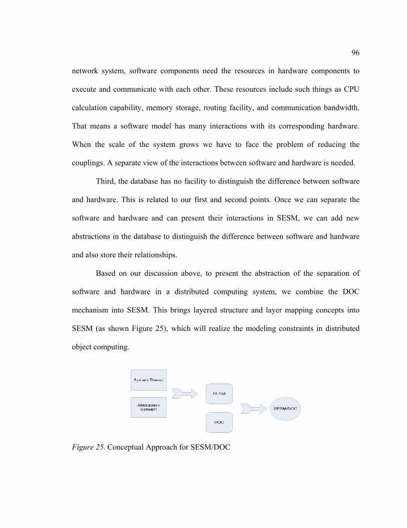
96
network system, software components need the resources in hardware components to
execute and communicate with each other. These resources include such things as CPU
calculation capability, memory storage, routing facility, and communication bandwidth.
That means a software model has many interactions with its corresponding hardware.
When the scale of the system grows we have to face the problem of reducing the
couplings. A separate view of the interactions between software and hardware is needed.
Third, the database has no facility to distinguish the difference between software
and hardware. This is related to our first and second points. Once we can separate the
software and hardware and can present their interactions in SESM, we can add new
abstractions in the database to distinguish the difference between software and hardware
and also store their relationships.
Based on our discussion above, to present the abstraction of the separation of
software and hardware in a distributed computing system, we combine the DOC
mechanism into SESM. This brings layered structure and layer mapping concepts into
SESM (as shown Figure 25), which will realize the modeling constraints in distributed
object computing.
Figure 25. Conceptual Approach for SESM/DOC

97
The following are the basic concepts that are defined for the layered structure
decomposition.
Notations:
Model Layer – ML
Mapping – M(MLs, MLh)
MLs–msoftware;
MLh – mhardware;
Definitions:
Model Layer (ML): In the co-design modeling approach, the software components
and hardware components belong to the software layer (MLs) and the hardware layer
(MLh). A model layer is defined as a group of models that share the same or similar
structural and behavioral properties. The models in the software layer have similar
structure and behavioral properties in that they all are in the computation domain and
they all have methods, tasks, and arcs (Butler, 1995). Each software component uses the
same means to communicate with the hardware components. Also all of them have to
load themselves into hardware. The hardware models in the hardware layer have
connections among themselves. They are all physical devices and have bandwidth and
computing and transportation capability. The models in one layer have a uniform way to
interact with the models in aother layer.
A model layer is different from a composite model. It has additional constraints
than a composite model. Models in a composite model do not need to share the same
structural or behavior properties. Component of a composite model can have coupling

98
relationships. A composite model allows its components to interact with models not in
the composite model. We have the following relationship for modeling the constraints
among the SESM/DOC models.
MLs ⊂ MB, MLh ⊂ MB,
∀ m ∈ MLs, m∉ MLh
∀ n ∈ MLh, n∉ MLs
Axiom:
Model Mapping: The concept of a model layer helps to separate the software
models and hardware models. So, instead of studying the interaction between individual
models in the software and hardware layers, emphasis is given to the interaction between
the layers. We call the relationship between layers mapping.
In co-design modeling, mapping is considered to be distinct from coupling.
Coupling entails information transportation between two models. In mapping, the
software component consumes the resources of a hardware component (e.g., CPU
computation power and memory). So, mapping is defined as an assignment relationship.
It is unidirectional. Mapping has more constraints than coupling. The mapping between
layers is unidirectional (from software layer to hardware layer). The cardinality of
mapping is “many to one” (that is, multiple software components can map to one
hardware component). Model mapping connects two model layers. For example, the
communication between two software models needs to go through the hardware layer by
system mapping. In the same layer, there may also exist direct interaction between
models, such as the coupling between two hardware models in a hardware layer. As both

99
individual models and ports can be the basic elements involved in model coupling, model
layers, individual models, and ports are needed as the basic elements to define mapping.
The model-layer mapping is realized by the mapping between individual models
belonging to different layers.
mi ∈ MLs, nj∈ MLh,
M(MLs,MLh) = {M(m1, n1), ..., M(mi, nj)}
M(m,n) = { )n ,(mC11 portInportOut1 , )n ,(mC
22 portInportOut2 ,…, )n ,(mCji portInportOuti }
Here, i and j are the number of the models involved in the mapping between the
software and hardware layers respectively.
Figure 26 shows the difference between model coupling and model mapping.
Model coupling presents the relationships between “ports”. Internal coupling shows the
information flow from one model’s output port to another model’s input port. External
coupling shows the information flow from either one model’s input port to another
model’s input port or one model’s output port to another model’s output port. Model
coupling describes the relationship between ports. When the concern is only for the
relationship between two models, coupling can be used to represent the general
connection between two models. For model mapping, it is the representation of the
assignment from one model layer to another model layer. The definitions and axioms
introduced in this chapter will be used in developing the SESM/DOC modeling approach.

100
Figure 26. Model Coupling and Model Mapping
4.3 Model Bases for Layered Structure Modeling
In SESM, there are three model bases for a designed model (MBTM, MBITM,
MBIM). These model bases separate models based on whether the model is a template
model, an instance template model or an instance model. In a co-design system, putting
all of the models that belong to different model layers into the model bases is not an
appropriate co-design. This section defines model bases that account for the above
requirements.
Modularity is an important feature in layered structure system modeling. It
provides clear boundaries to different layers. In SESM/DOC, we define multiple model
bases for distributed object computing system modeling. Inherent with SESM,
SESM/DOC has the facilities to create a Template Model (TM), an Instance Template

101
Model (ITM), and a Model Instance (MI). Inherent with DOC, the three layers specified
in DOC are supported by SESM/DOC.
Software layer (SESM/DCO): alternative software design models are supported
using a predefined software model with constraints on its execution on specific hardware
components.
Hardware layer (SESM/LCN): alternative hardware design models are supported
using a predefined collection of hardware model components that comply with
constraints that dictate which model components may be connected to one another.
Object System Mapping (SESM/OSM): alternative co-design models are
supported under a set of constraints that dictate legitimate software to hardware mappings
Each of these has its own model types and model constraints. For the multiple
model bases of a distributed object computing system, the first level of multiple model
bases will be the software model base (SMB), the hardware model base (HMB), and the
object system mapping model base (OMB). In each of the above model bases, there are
three sub-models according to the separated layers – the template model, the instance
template model and the instance model. So, for software models, there are the software
template model base (SMBTM), the software instance template model base (SMBITM), and
the software instance model base (SMBIM). In total, nine model bases are defined to
support distributed co-design modeling, as shown in Table 11.

102
Table 11
Multiple Model Bases for Distributed Object Computing System
Software Model Hardware Model Object Mapping Template Model SMBTM HMBTM OMBTM
Instance Template Model SMBITM HMBITM OMBITM Instance Model SMBIM HMBIM OMBIM
4.3.1 Model Types for Co-design
As discussed in Chapter 3, a distributed object computing system has its own
elements. When we combine SESM and DOC, these DOC elements should be classified
into SESM model bases. To handle large-scale and complex systems, a “Group Model”
concept is defined as a composite model which contains the same types of models. We
introduce the model types based on their model bases.
Hardware Layer Model Types
According to DEVS/DOC specification, SESM/DOC supports the following
hardware models:
1. Hardware Layer Model (HLM);
2. Processor (which includes CPU, Routing Unit, Transport Unit) Model (PM);
3. Network Interface Model (NIM);
4. Link Model (LM);
5. Router Model (RM);
6. Processor Group Model (PGM);
7. Network Interface Group Model (NIGM);

103
8. Link Group Model (LGM);
9. Router Group Model (RGM);
10. Processor and Network Interface Model (PNM);
11. Processor and Network Interface Group Model (PNGM).
Software Layer Model Types
Software layer in DEVS/DOC specification has two model types:
1. Software Layer Model (SLM); 2. Software Application Model (SAM)
SLM is a composite model which is composed from one or more SAMs. Each
SAM is a primitive model which represents the abstraction of a software application
which can run on an appropriate hardware component.
Object System Mapping Model Types
Unlike the software layer and hardware layers, the OSM layer is not a physical
layer. It represents the abstraction of mapping from the software layer to the hardware
layer in DEVS/DOC. It supports three model types: SLM, HLM and the system model.
The first two model types are defined in previous chapters. The last one is a SESM
composite model with certain constraints. For example, the mapping direction can only
go from the software layer to the hardware layer.

104
Beside the above model types, modelers can define their own model types based
on the system that is to be modeled. These user-defined model types should work
together with the pre-defined model types.
4.3.2 Network System Model Constraints
It is important for a modeling approach and its realization to define constraints on
composite model specifications. For example, a model may not contain other models as
components or only certain types of models may be connected. DOC, as a layered
distributed system design specification, brings co-design modeling constraints to SESM.
In DOC’s layered structure, we have a set of model types for describing software and
hardware aspects of a distributed network system as described above. These model types
are abstractions of particular entities, such as software application or router. Their
structures and behaviors are defined according to the DOC and DEVS specifications.
To support co-design model specification, the SESM framework is extended to
support the DOC model typing and constraints. The model typing in SESM/DOC entails
three sets of model constraints. One is the composition relationship between two models
that answers the question of which model can contain or be contained by which other
kinds of models. The second set is the coupling relationship between two models that
answers the question of which two model types can be connected (coupled). These
constraints guarantee the right relationship between different DOC models according to
the predefined model types. The third set is the mapping relationship between two model
layers that answers the question about model assignment for co-design.
105
Hardware Layer Model Constraints
SESM/DOC supports the following composition constraints.
1. HLM can contain only group models (PGM, NIGM, LGM, RGM);
2. PGM can contain only PM;
3. NIGM can contain only NIM;
4. LGM can contain only LM;
5. RGM can contain only RM;
6. PNGM can contain only PNM;
7. PNM can contain only one PM and one NIM;
8. RM, NIM, LM, RM are primitive models
These model types and the connections between them will present different
network topologies. In SESM, the connections are represented by couplings. The
connection constraints between different model types are implemented by model
coupling constraints as follows:
1. HLM can be coupled only with group models
2. PM can be coupled only with PGM;
3. NIM can be coupled only with NIGM;
4. LM can be coupled only with LGM;
5. RM can be coupled only with RGM;

106
6. RGM can be coupled only with RM and NIGM;
7. NIGM can be coupled only with NIM, RGM, LGM, PM, PNGM and RGM;
8. LGM can be coupled only with NIGM;
9. RGM can be coupled only with NIGM.
Software Layer Model Constraints
SESM/DOC supports the following model composition constraints in software
layer:
1. SLM can only contain SAM;
2. SLM has to contain at least one SAM;
3. SAM is a primitive model.
SESM/DOC also supports the following model coupling constraints in the
software layer:
1. SLM can only be coupled with SAM
2. SAM can only be coupled with SLM
Object System Mapping Model Constraints
The composite constraint in the OSM states that the system model contains and
only contains one SLM and one HLM. The mapping constraint in OSM states that the
only mapping in the system model is the mapping from SLM to HLM.

107
With SESM/DOC, modelers are given the flexibility to define their own models.
Modelers can define new models for computer network applications such as the search
engine network described earlier in this chapter. Even for distributed object computing
co-design, they can still redefine the model components and create different groupings.
For example, in the above hardware models we have a processor model (PM) and a
network interface card model (NIC). These two models can be combined as a
processorNIC model. This assumes each processor has one network interface card to
connect to the network. Accordingly, the hardware constraints need to be adopted to
match the hardware layer model types.
4.4 Summary
In this chapter, a component-based layered structure modeling approach is
presented for co-design modeling of distributed network systems. Model layer and model
mapping concepts are defined to specify the separation and synthesis of software and
hardware components for the co-design modeling. Based on the DOC abstract model, a
set of new model types are defined for the software and hardware parts of a distributed
system. The group model concept is defined to help organize the same type of models.
Based on these model types, a set of model constraints are specified to guarantee the
correctness of the structure of the co-design network models. Multiple model bases are
defined to support different model resolutions appropriate for software/hardware co-
design system modeling.

108
Compared to the other modeling approaches discussed in Chapters 2 and 3, the
layered structure modeling approach provides a well-defined specification for the
separation and synthesis of the software and the hardware model components. This
specification gives the software models and the hardware models distinct boundaries, so
that they can be separately defined, developed, and synthesized. The software and
hardware co-design provides a set of well-defined model components and relationships to
specify distributed computer network systems.
This specification is based on co-design modeling concepts and model types. The
logical layered structure modeling approach presented here provides the basis for
developing the visual and persistent modeling capabilities described in Chapter 5.

5 CO-DESIGN VISUAL AND PERSISTENT MODELS PRESENTATION FOR
NETWORK SYSTEMS
Visual modeling is an intuitive way for modelers to specify logical models. Visual
modeling languages can enforce syntax and semantics of modeling formalisms such as
DEVS/DOC (Burmester, Giese, & Henkler, 2005; Harel, 1987; Object Management
Group, 2007; Sarjoughian, 2001). It is also good for the people who do not want to go to
the code level to design models. Persistent modeling is a modeling approach that uses a
database for model repository. It affords large-scale model management and helps with
the model reusability and model structural complexity measurement. Co-design model
representation and repository are very important in separating the design and repository
of the software layer and the hardware layer in network system. Current modeling
approaches do not visually separate the design of the software and hardware models for a
network system and do not store/manage the co-design models in a database as supported
in SESM. In this chapter, the approach for the co-design modeling visual representation
and repository for network systems will be presented.
5.1 Visual Modeling
The co-design visual modeling needs to represent two kinds of information: the
model components and the relationships between the model components. To visually
present the logical models defined in Chapter 4, the SESM visual modeling approach is
extended to be used in SESM/DOC.

110
5.1.1 Model Components
Based on this discussion, we will use the visual modeling elements of SESM to
represent the primitive and composite logical model components defined in Chapter 4.
The block diagram in SESM can be used both in primitive and coupled models, as shown
in Figure 27. In Figure 27, there are three models, two primitive “Router” models, and
one composite “RouterGroup” model.
Figure 27. Block Diagram Visual Model
For large-scale and complex distributed object computing systems, the number of
system entities can be large. For example, in a distributed network system, there may be
hundreds of processors and hundreds of routers. To present all of these models one by
one is impractical given the limitations of visual space on the computer screen. In
SESM/DOC, it is important to visually create a group model to group the same kind of
models, such as the “LinkGroup01” shown in Figure 28, which groups five “Link01”
models. This helps to organize the models with the same model type.

111
Figure 28. Link Group Model
5.1.2 Model Relationship
In both SESM and DEVS/DOC, the relationship between two models is presented
by coupling. In SESM, the coupling in SESM is a dashed line with an arrow pointing to
the direction of the information. For complicated systems, there are usually more
connections between models and this could require many couplings. As described in
Chapter 3, visual representation of a large number of couplings in a composite model can
be difficult to view. It is important to organize the model couplings so that the model
view is clear in a limited visual space. In SESM/DOC the approaches to reduce the
number of couplings uses the concepts of the integrated port and bidirectional
connection.
A model can have many ports which can lead to many couplings to other models.
In SESM/DOC, the coupling relationship is based on the logical model presented in
Chapter 4, so one integrated port can be created to identify which model is involved in
the coupling relationship. In SESM and DEVS, the coupling relationship is tightly related
112
to the model ports. For internal coupling, the coupling has to be from one output port to
one input port. For external coupling, the coupling has to be either from one input port to
another input port or one output port to another output port. To show the connection
relationship between models using the non-arrowed segmented line, we do not need to
know the about the input or output ports. The only thing we need to know is from/to
which model we are connecting. So in SESM/DOC, a model only needs to have one kind
of port, the identity port which integrates at least one component port to be used for the
model connection. This port is defined as an integrated port. This integrated port
integrates all of the ports of the model (Xie, 2004). For the integrated port, the arrowed
dashed line in SESM is not sufficient to present the information flow, so in SESM/DOC,
a bidirectional information flow is presented using a non-arrow dashed line.
In order to make the visual model easy to read for a primitive model, we design
two integrated ports: one on its left and one on its right. Each of them is both input port
and output port. For a composite model, depending upon the components it has, it can
have multiple ports which can be connected to its components and other models. The
integrated port and bidirectional coupling approaches reduce the complexity in visual
model design by reducing the number of couplings. The model connection tells which
models are involved in a particular model connection, as shown Figure 29.

113
Figure 29. The Non-arrowed Segment Line for Model Connection
In Figure 30, two features of SESM/DOC are presented. The first one is the
grouping model which is the composite model including multiple same type models. For
example, LinkGroup01 has five link models inside it. The second feature is the non-
arrowed dashed line showing the connections. The connection among hardware in DOC
gives the topology of the distributed network. The grouping model helps to organize the
visual model deployment and helps to reduce the complexity. In the OSM model layer,
the mapping relation has an arrow to show how a software model is mapped onto a
hardware model through the identity port of a software layer and the integrated port of a
hardware layer, as shown in Figure 30.
Figure 30. OSM Model

114
Every dashed arrowed line in the mapping relationship is not trivial. For example,
the system in Figure 31 is a different from the system shown in Figure 30. There are two
software applications (SoftwareApplication03 and SoftwareApplication04) running in the
same processor (the first processor02 model in processor group) in Figure 31. That means
the CPU and memory in the processor will be shared by two software applications. In
Figure 30, however, each software application runs on its own processor. This
visualization of model connections significantly reduces the complexity of the system
model for a large-scale and complex system, and makes a graphical representation of the
models simpler to view and manipulate. In next chapter we will show examples of visual
models for the search engine network system.
Figure 31. Alternative OSM Model
5.1.3 Tree Structure and Block Diagram Views
Besides the block diagram model we saw above, SESM/DOC also provides a tree
structure view of models, as shown in Figure 32. In the tree structure view, every model
in the mode base is a node. The primitive ones are the leaves of the tree. From the tree
structure view, it is easy to tell the model relationships across multiple levels, while in a
block diagram view, the composite model’s component and their relationships can be

115
viewed. The information of the model specialization relationship is presented in both the
tree structure and the block diagram. In the former, the letter “S” is used for identify
specialized models. In the block diagram and the tree structure different colors are used
to help identify models. In Figure 33 we can see the Processor02 model is specialized as
a singleCoreProcessor and doubleCoreProcessor which are both Processor02 but with
different properties.
Figure 32. SESM Model Tree Structure
Figure 33. Model Specialization

116
5.1.4 Multiple Layer Model Representation
To support the DOC abstract model in SESM, separating the visual models for
software and hardware layers is important. It is necessary to have distinct views of the
layers. When a modeler is working in a software section, all of the model candidates in
the current model tree are software models. This should also be true for hardware models.
Based on the separation of the logical software and hardware model layers, SESM/DOC
provides three working sections for the visual model representation: the software model
working section, the hardware model working section, and the system model working
section. The system modeler can switch among these three sections as needed. Each of
the sections has a unique block diagram and model tree (the software, the hardware and
the system tree structure), as shown in Figure 34.
Figure 34. Multiple Sections for Visual Modeling
In Figure 34, the current section is for the software layer. All of the models
created and edited in this section are software models. The modeler will not have access
to hardware or system models. This ensures that the modeler will not mistakenly define
software, hardware and system models.
117
5.2 Model Persistence
As described in Chapter 3, SESM stores all of the logical models in its database.
This is a much better approach than the file system in DEVS/DOC where models are
saves as individual files. From a modeler’s perspective, it is difficult to see the
relationship between models through a file system. According to the separation of the
logical model and in order to provide the modularity and be consistent with the model
constraints for system co-design discussed in Chapter 4, SESM/DOC provides three sets
of database tables for software, hardware, and system models. This separation in the
database systematically manages the DOC abstract model for both the logical and visual
models.
Figures 35, 36, and 37 show database schema designs that are extended for DOC
models (Elamvazhuthi, Sarjoughian, & Hu, 2007).

118
NSMTemplatensmID : INTEGERcreateTime : DOUBLE PRECISION
<<PK>> PK_NSMTemplate53()
componentOfItOwner : VARCHAR(50)tiOwner : INTEGERiOwner : INTEGERtComponent : VARCHAR(50)tiComponent : INTEGERiComponent : INTEGER
<<FK>> FK_componentOfI83()<<PK>> PK_componentOfI57()<<FK>> FK_componentOfI98()<<Unique>> TC_componentOfI403()
IMtemplate : VARCHAR(50)templateI : INTEGERiID : INTEGERmodelName : SMALLINTcreateTime : DOUBLE PRECISION
<<PK>> PK_modelInstance43()<<FK>> FK_modelInstance69()<<FK>> FK_modelInstance81()
1
0..*
1
0..*
Owner/Composite Models
<<Identif y ing>>
ITMtoSMItTemplate : VARCHAR(50)tiTemplate : INTEGERtSpecialization : VARCHAR(50)tiSpecialization : INTEGERiSpecialization : INTEGERname : VARCHAR(1)type : VARCHAR(1)Type_tID : VARCHAR(50)
<<FK>> FK_MTItoSMI68()<<PK>> PK_MTItoSMI44()<<FK>> FK_MTItoSMI92()<<Unique>> TC_MTItoSMI390()
0..1
1
0..1
1
<<Identifying>>
componentOftOwner : VARCHAR(50)tComponent : VARCHAR(50)tiComponent : INTEGERname : VARCHAR(1)type : VARCHAR(1)Type_tID : VARCHAR(50)
<<FK>> FK_componentOf59()<<PK>> PK_componentOf39()<<FK>> FK_componentOf65()
ITMtID : VARCHAR(50)tiID : INTEGERcreateTime : DOUBLE PRECISIONname : VARCHAR(1)type : VARCHAR(1)Type_tID : VARCHAR(50)
<<PK>> PK_ModelTI38()<<FK>> FK_ModelTI62()<<FK>> FK_ITM109()
1 0..11 0..1
<<Identifying>>
1
0..*
1
0..*
<<Identifying>> 1
0..*
1
0..*
<<Identifying>>
specializationtemplate : VARCHAR(50)
<<PK>> PK_specialization13()<<FK>> FK_specialization40()
stateVariablesowner : VARCHAR(50)varName : VARCHAR(50)varValue : VARCHAR(255)varType : VARCHAR(1)modelType : VARCHAR(3)
<<PK>> PK_stateVariables8()<<FK>> FK_stateVariables94()<<FK>> FK_stateVariables106()
0..*
0..1
<<PartiallyDepende...
Ty pename : VARCHAR(50)ty pe : VARCHAR(1)
<<PK>> PK_Ty pe59()<<FK>> FK_Ty pe111()<<Unique>> TC_Ty pe476()
TMtID : VARCHAR(50)tModelType : VARCHAR(50)createTime : TIMESTAMP
<<PK>> PK_ModelTemplate1()<<Unique>> TC_ModelTemplate1()
1
0..*
1
0..*
<<Identifying>>1
1..*
1
1..*
<<Identif y ing>>
1
0..*
1
0..*
<<Identifying>>
0..*
1
0..*
1
<<Identifying>>
1
1
1
1<<Identifying>>
Figure 35. DOC Data Schema - Kernel

119
couplingtOwnerF : VARCHAR(50)tNameF : VARCHAR(1)tTy peF : VARCHAR(50)tiOwnerF : VARCHAR(1)name : VARCHAR(1)tOwnerT : VARCHAR(50)tNameT : VARCHAR(1)tTy peT : VARCHAR(50)tiOwnerT : VARCHAR(1)
<<FK>> FK_coupling56()<<PK>> PK_coupling47()<<FK>> FK_coupling97()<<Unique>> TC_coupling401()
IPTtOwner : VARCHAR(50)tName : VARCHAR(1)tTy pe : VARCHAR(50)tiOwner : VARCHAR(1)
<<PK>> PK_PortTI34()<<FK>> FK_PortTI55()
10..* 10..*
FromCoupling
<<Identifying>>
11
11
ToCoupling
<<Identifying>>
PTowner : VARCHAR(50)tName : VARCHAR(1)tTy pe : VARCHAR(50)createTime : DOUBLE PRECISION
<<PK>> PK_PortTemplate32()<<FK>> FK_PortTemplate53()
1
1..*
1
1..*
<<Identifying>>
stateVariablesowner : VARCHAR(50)v arName : VARCHAR(50)v arValue : VARCHAR(255)v arTy pe : VARCHAR(1)modelTy pe : VARCHAR(3)
<<PK>> PK_stateVariables8()<<FK>> FK_stateVariables94()<<FK>> FK_stateVariables106()
StatisticstModelType : VARCHAR(50)numChildren : INTEGERtotalChildren : INTEGERinPort : INTEGERoutPort : INTEGEReic : INTEGEReioc : INTEGERic : INTEGERname : VARCHAR(50)
<<PK>> PK_Statistics27()<<FK>> FK_Statistics43()
TMtID : VARCHAR(50)tModelTy pe : VARCHAR(50)createTime : TIMESTAMP
<<PK>> PK_ModelTemplate1()<<Unique>> TC_ModelTemplate1()
1
0..*
1
0..*
<<Identifying>>
1
0..*
1
0..*
<<Identifying>>
1
1
1
1
Stats Info
<<Identifying>>
Figure 36. DOC Data Schema – Ports, Coupling, State Variable and Statistics
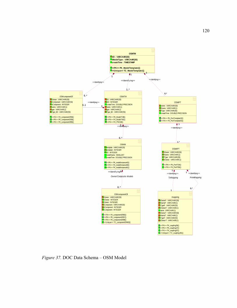
120
OSMcomponentOfItOwner : VARCHAR(50)tiOwner : INTEGERiOwner : INTEGERtComponent : VARCHAR(50)tiComponent : INTEGERiComponent : INTEGER
<<FK>> FK_componentOfI83()<<PK>> PK_componentOfI57()<<FK>> FK_componentOfI98()<<Unique>> TC_componentOfI403()
OSMIMtemplate : VARCHAR(50)templateI : INTEGERiID : INTEGERmodelName : SMALLINTcreateTime : DOUBLE PRECISION
<<PK>> PK_modelInstance43()<<FK>> FK_modelInstance69()<<FK>> FK_modelInstance81()
1
0..*
1
0..*
Owner/Composite Models
<<Identif y ing>>
OSMcomponentOftOwner : VARCHAR(50)tComponent : VARCHAR(50)tiComponent : INTEGERname : VARCHAR(1)type : VARCHAR(1)Type_tID : VARCHAR(50)
<<FK>> FK_componentOf59()<<PK>> PK_componentOf39()<<FK>> FK_componentOf65()
OSMITMtID : VARCHAR(50)tiID : INTEGERcreateTime : DOUBLE PRECISIONname : VARCHAR(1)type : VARCHAR(1)Type_tID : VARCHAR(50)
<<PK>> PK_ModelTI38()<<FK>> FK_ModelTI62()<<FK>> FK_ITM109()
10..1 10..1<<Identifying>>
1
0..*
1
0..*
<<Identifying>>
OSMTMtID : VARCHAR(50)tModelType : VARCHAR(50)createTime : TIMESTAMP
<<PK>> PK_ModelTemplate1()<<Unique>> TC_ModelTemplate1()
1
0..*
1
0..*
<<Identifying>>
1
1..*
1
1..*
<<Identif y ing>>
OSMPTowner : VARCHAR(50)tName : VARCHAR(1)tType : VARCHAR(50)createTime : DOUBLE PRECISION
<<PK>> PK_PortTemplate32()<<FK>> FK_PortTemplate53()
1
0..*
1
0..*
<<Identifying>>
OSMIPTtOwner : VARCHAR(50)tName : VARCHAR(1)tType : VARCHAR(50)tiOwner : VARCHAR(1)
<<PK>> PK_PortTI34()<<FK>> FK_PortTI55()
1
1..*
1
1..*
<<Identifying>>
mappingtOwnerF : VARCHAR(50)tNameF : VARCHAR(1)tTypeF : VARCHAR(50)tiOwnerF : VARCHAR(1)name : VARCHAR(1)tOwnerT : VARCHAR(50)tNameT : VARCHAR(1)tTypeT : VARCHAR(50)tiOwnerT : VARCHAR(1)
<<FK>> FK_coupling56()<<PK>> PK_coupling47()<<FK>> FK_coupling97()<<Unique>> TC_coupling401()
1
0..*
1
0..*
FromMapping
<<Identifying>>1
1
1
1
ToMapping
<<Identifying>>
Figure 37. DOC Data Schema – OSM Model
121
Figure 35 shows the kernel data schema for software models and hardware
models. In this figure, the “TM” stores the template models for software or hardware
models. For example, the decomposition relationship for a composite model is stored in
the table of “componentOf”. The “ITM” table has the records of the instance template
model discussed in the Chapter 3. The “Type” table has the network systems co-design
model typing information which enforces the network systems co-design modeling
constraints. Every composition relationship and coupling relationship will be checked
again this “Type” table to guarantee the correct model type is used. Figure 35 also shows
the specialization information and the state variables are also stored in the data tables.
Figure 36 provides the data schema with the model ports, couplings and state
variables. It also contains the structural complexity metrics for one of the software,
hardware, or system models in the “Statistics” table which is in charge of the
measurement of co-design system structural complexity based on quantity information
such as the number of model components, the number of model ports, and the number of
couplings.
The OSM data schema is similar to the software and hardware data schema but
with some differences. As shown in Figure 37, the OSM data schema does not have a
coupling table. It has a “mapping” table which stores alternative software models to
hardware models assignments as shown in Table 12. The components of the OSM
template model are the models chosen from the software and hardware layer.

122
Table 12
OSM Mapping Table
The specifications of this mapping table is:
1. “mapping” table is the table for object system mapping model mapping
2. “OSMtOwnerF” is a foreign key referring to “OSMname” from
OSMmodelTemplate. It is the name of the model from which the mapping
starts.
3. “OSMtiOwnerF” is a foreign key referring to “OSMtiID” from OSMmodelTI.
4. “OSMtNameF” is a foreign key referring “name” from OSMportTemplate. It
is the name of the port from which the mapping starts.
5. “OSMtTypeF” a foreign key referring to “OSMtType” from
OSMportTemplate.
6. “OSMtOwnerT” is a foreign key referring to “OSMname” from
OSMmodelTemplate. It is the name of the model at which the mapping ends.
7. “OSMtiOwnerT” is a foreign key referring to “OSMtiID” from OSMmodelTI.
8. “OSMtNameT” is a foreign key from referring to “OSMtName” from
OSMportTemplate. It is the name of the port at which the mapping ends.
9. “OSMtTypeT” a foreign key referring to “OSMtType” from
OSMportTemplate.
mapping
OSMtOwnerF OSMtiOwnerF OSMtNameF OSMtTypeF OSMtOwnerT OSMtiOwnerT tNameT tTypeT

123
10. The primary key is a multiple-field primary key which includes “OSMtOwnerF”,
“OSMtiOwnerF”, “OSMtNameF”, “OSMtTypeF”, “OSMtOwnerT”,
“OSMtiOwnerT”, “OSMtNameT”, and “OSMtTypeT”.
Figures 35, 36, and 37 show that SESM/DOC almost triples the number of tables
in SESM to separate the persistent models of the software, hardware, and object system.
However, they are not mere duplications. Based on the SESM/DOC constraints we
discussed above, the model typing issues play an important role in the database. In other
words, the SESM/DOC database needs to guarantee the model typing correctness. Also,
the separation of the DCO, LCN, and OSM models in different tables provides the
modularity for persistent model manipulation. When the hardware schema is changed, the
model data of the software model and the system model will not be affected.
In the SESM/DOC database, the DOC constraints are guaranteed by two typing
tables: software type table and hardware type table, as shown in Tables 13 and 14. Each
of the tables has two columns, one is for the model ID and the other is for the model
types.
Table 13
Software Model Type Table
SWModelID SWModelType
Text File Server SOFTWARE Two Servers Two Clients Software Layer SWLAYER … …
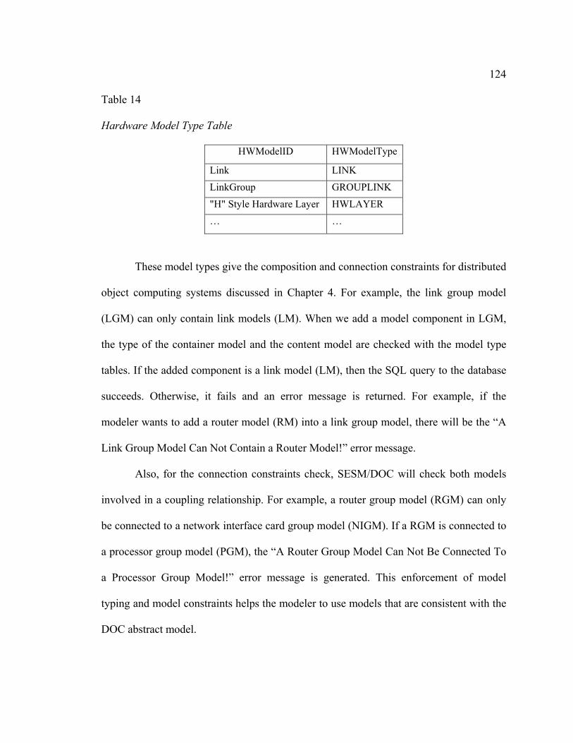
124
Table 14
Hardware Model Type Table
HWModelID HWModelType
Link LINK LinkGroup GROUPLINK "H" Style Hardware Layer HWLAYER … …
These model types give the composition and connection constraints for distributed
object computing systems discussed in Chapter 4. For example, the link group model
(LGM) can only contain link models (LM). When we add a model component in LGM,
the type of the container model and the content model are checked with the model type
tables. If the added component is a link model (LM), then the SQL query to the database
succeeds. Otherwise, it fails and an error message is returned. For example, if the
modeler wants to add a router model (RM) into a link group model, there will be the “A
Link Group Model Can Not Contain a Router Model!” error message.
Also, for the connection constraints check, SESM/DOC will check both models
involved in a coupling relationship. For example, a router group model (RGM) can only
be connected to a network interface card group model (NIGM). If a RGM is connected to
a processor group model (PGM), the “A Router Group Model Can Not Be Connected To
a Processor Group Model!” error message is generated. This enforcement of model
typing and model constraints helps the modeler to use models that are consistent with the
DOC abstract model.

125
Besides checking the composite and connection constraints, a model type is also
important in object system mapping. In Chapter 6, when a system model is created, only
one software layer model and one hardware layer model can be added as the system
model’s components. Furthermore, only a software layer model and a hardware layer
model can be involved in a system mapping relationship. For example, if we try to map
two hardware layer models, an error message will be generated.
The new database schema in SESM/DOC helps the modeler with model
development and management. The separated database table sets provide the modularity
for co-design persistent modeling because once software model or hardware model types
or constraints change, they will not affect each other. Therefore, new model types can be
added into the model type table. This helps SESM/DOC to be extended in future.
5.3 Summary
This chapter provides the visual and persistent modeling capabilities that are
necessary for network system co-design. The visual modeling approach enables the visual
separation and synthesis of different model layers defined in Chapter 4. The separate
working sections are defined to help with the software/hardware visual model designs. To
deal with the scalability and structural complexity of model visualization, the
bidirectional model coupling, integrated port and group model concepts are developed.
This approach reduces the complexity for large-scale network system modeling and
reduces the difficulty modelers could experience when there are a large number of
couplings. Database schemas are developed to separate the models in the software, the

126
hardware, and the system model layers. The mapping table in the OSM schema supports
synthesis of the software and hardware models. The software model and hardware model
type tables help ensure co-design modeling relationships are defined. The tables also
support the obtainment of the structural complexity metrics for the software, hardware,
and system models.

6 DISTRIBUTED CO-DESIGN MODELING EXAMPLE
In this Chapter, the distributed co-design modeling example of the search engine
system mentioned in Chapter 4 will be used to show how the capabilities of the
SESM/DOC modeling environment helps a modeler to develop a distributed network
system.
6.1 The Search Engine Network System Problem
The co-design modeling approach developed in Chapters 4 and 5 is used for the
search engine system described next. A search engine network is an interesting system to
be modeled and simulated (see Figure 38). To analyze or design this search engine
network system, one needs to consider the software applications, the network hardware,
and how they can be synthesized. The details specific to the software, the hardware and
the assignment of software on hardware determine important aspects of the system such
as performance (i.e., percentage of successful data transmission). This requires the
modeling of such system to separate the software parts and hardware parts.
Figure 38. Search Engine Network System

128
A simplified search engine network system is shown in Figure 38. Because the
topology of this network example looks like a letter “H”, it is called an “H” style network
system. In Figure 38, there are search engine servers which provide the search results,
clients who make search requests, and the network between the servers and clients. The
servers and clients are composed of both software and hardware. The clients use some
designated software to make the search requests. Then, these requests go through the
links and arrive at servers through the network routers. Depending on different search
keywords in the requests, the requests will be directed to specific servers which are in
charge of handling different categories of search requests, including the particular search
key word. For example, the request “African Mountain” will be directed to the server
which is in charge of the index from “A” to “L”.
In order to narrow the search range and get the most related search results faster,
the clients can add more key words, such as “African Mountain” plus “English”, meaning
the search is about the English file for “African Mountain”. The software in the server
handles the search requests. Different requests (classified by their keywords) received by
the same server will be treated by different applications within the server. For example,
the search of “African Mountain” plus “English” and “African Mountain” plus “Chinese”
will be treated by different applications in the same server.
In Figure 38, there are there are two search engine servers that provide searching
services. Here we choose Figure 38 as an example to develop the distributed co-design
model in SESM/DOC. As discussed in Chapter 4, clients use their software to make the

129
search requests. In response to the different requests received, the server will provide
different searching results.
Different server methods are used to provide different responses in order to
narrow the search range and get the most related search results faster. In our example,
one server is in charge of the video request and the other is in charge of the text request.
Alternative hardware configuration and topology also change the network performance.
6.2 Model Design
Models are designed in different working sections in SESM/DOC. First, the
hardware and software component models are defined. Then, the model relationship
between the hardware and software models is given.
6.2.1 Primitive and Composite Components
For this search engine network system, we need to begin by classifying which
parts of the system should be modeled as “software” and “hardware” components. The
classification work can be done based on the DOC, LCN, and OSM layers defined in
earlier chapters. As we discussed in Chapter 5, in SESM/DOC we provide some grouping
models to help integrate the same type of models, which make the visual models simpler
to view. For system model integration, we provided a “software layer model” and a
“hardware layer model” which are the basic elements for the OSM model. Based on the
DOC abstract model in Chapter 3 and the logical model in Chapter 4, we have the
candidate models shown in Table 15.
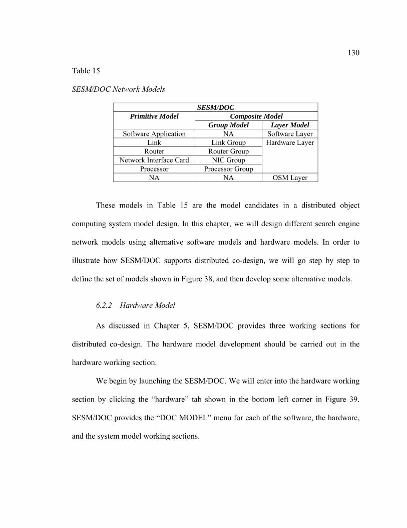
130
Table 15 SESM/DOC Network Models
SESM/DOC Composite Model Primitive Model
Group Model Layer Model Software Application NA Software Layer
Link Link Group Router Router Group
Network Interface Card NIC Group Processor Processor Group
Hardware Layer
NA NA OSM Layer
These models in Table 15 are the model candidates in a distributed object
computing system model design. In this chapter, we will design different search engine
network models using alternative software models and hardware models. In order to
illustrate how SESM/DOC supports distributed co-design, we will go step by step to
define the set of models shown in Figure 38, and then develop some alternative models.
6.2.2 Hardware Model
As discussed in Chapter 5, SESM/DOC provides three working sections for
distributed co-design. The hardware model development should be carried out in the
hardware working section.
We begin by launching the SESM/DOC. We will enter into the hardware working
section by clicking the “hardware” tab shown in the bottom left corner in Figure 39.
SESM/DOC provides the “DOC MODEL” menu for each of the software, the hardware,
and the system model working sections.

131
In the hardware working section, one can click “DOC MODEL”, and choose to
create a predefined hardware template model. The hardware model types defined in
Chapter 4 are shown as the model candidates. Once a model template is chosen, a name
for this hardware template model must be entered. This name will be saved in the
database as this model’s ID (the ID for the template model is the primary key in the
template model table). Also, once a model type is chosen, the model type is stored so that
this model has the appropriate model constraints defined for it (see Chapter 4). We
choose to create a processor and give the name, “SearchProcessor”, as shown in Figure
39.
Figure 39. Primitive Hardware Model Development
For this processor model, we add integrated ports to it. For name convention, the
group model ports are named as “xx*P?”. Here “xx” means the abbreviation of the group
(for example, LinkGroup is LG). The symbol “*” indicates if the port is on the left or
right in the visual graphic model. The symbol “?” represents the port number. “SPLP”

132
means “SearchProcessor Left Port”, and, “SPRP” means “SearchProcessor Right Port”.
The ports can be added through the “add port” function in the “Edit” menu bar or through
the tree structure and block views.
Composite models can be created based on the primitive models. We create a
processor group model to combine all of the processors needed in the search engine
network system model. Following the same steps of creating a primitive template model,
we have a “ProcGroup” processor group model. Now one can add processor components
into this processor group model from a drop down list, as shown in Figure 40.
Figure 40. Adding Hardware Components into Hardware Group Model
When any component model is added, the model composite constraints discussed
in Chapter 4 are checked to see whether this operation will violate any model composite
constraints. According to the hardware model composite constraint “PGM can only
contain PM”, there is no violation and the processor models can be successfully added as

133
components in processor group model. Otherwise, the add operation fails and an error
message will be shown as “DOC Composite Constraint Violation: A PGM can only
contain PM”.
We add four processors and specify the couplings among the processors and the
processor group. As the hardware composite constraints are checked, the hardware
coupling constraints are also checked to ensure the coupling relationship is correct.
Otherwise, the coupling operation fails and an error message will be displayed.
According to the hardware model coupling constraints in Chapter 4, the couplings
between processors and processors and the processor group are correct. So, the complete
processor group is created as shown in Figure 41.
Figure 41. Hardware Group Model
In Figure 38, the network system uses both “star” and “bus” topologies. We name
the hardware layer model after the “H” system, as shown in Figure 42. In Figure 42, we
see all the group models and their coupling relationships. The group model defined in

134
Chapter 4 contains the same types of models. Figure 43 shows the instance template
model tree structure. From Figure 43 we can see in the NIGM named “NICGroup”, there
are 10 network interface cards and 3 specializations. The letter “u” after the specialized
model name indicates that the model has not chosen which specialization will be used.
These 10 network interface cards are in Figure 38. They are coupled with links,
processors and routers to build up the search engine system shown in Figure 38. In fact,
with the group modeling and model coupling approaches, SESM/DOC can design any
topology for computer network systems. Using the integrated ports and bidirectional
dashed lines, the model visual presentation is clear for a large number of models.
Figure 42. “H” Style Hardware Layer

135
Figure 43. Instance Template Model Tree Structure for “H” Style Hardware Model
Figure 44 is an alternative hardware topology of the search engine network. Based
on the shape of the network, as we did for “H” style network, we name this alternative
one “I” style. This network has the same functionality as the one in Figure 38. The only
difference is the network topology.
Figure 44. “I” Style Network System

136
The model of the “I” style hardware network is shown in Figure 45. This model
has the “I”NICGroup model instead of the NICGroup model in the “H” style network.
Also, the “I”LinkGroup replaces the LinkGroup model and the “I”RouterGroup replaces
the RouterGroup model.
Figure 45. “I” Style Hardware Layer
For these two different networks, using SESM/DOC complex metrics, we can
obtain an analysis to compare the two hardware models. Figure 46 shows the structural
complexity metrics of “H” style hardware models and Figure 47 shows the structural
complex metrics of “I” style hardware models.

137
Figure 46. Structural complexity Metrics for “H” Style System
Figure 47. Structural complex Metrics for “I” Style System
From the two metrics, we can see that complexity of the “I” style is smaller than
the “H” style. For example, the total number of models in “I” style is 17 while the “H”
style has 25. Furthermore, the “I” style has 16 total couplings while the “H” style has 24
couplings. We examine the performance differences of these two models after they are
simulated.

138
SESM/DOC provides the model specialization facility. It is important for the
models to share the same structural properties and yet have different behavioral
properties. For example, as mentioned in Chapter 3, the network interface card (NIC)
model is in charge of the network CSMA/CD (Carrier Sense Multiple Access with
Collision Detection) protocols for the network model. The CSMA/CD protocol varies
with different back off schemas: random back off schema (RBO), also called “Binary
Exponential Back off Schema”, one by one back off schema (OBOA), and one by one
back off schema (OBOB). Based on the different back off schema, the NIC model can be
specified with one of three specifications: NIC_RBO, NIC_OBOA and NIC_OBOB, as
shown in Figure 48.
Figure 48. Hardware Specialization

139
To differentiate the specification for the network interface cards, we add the state
variable “BackOffMode” into the NIC and give it different values. For example, for
“NIC_OBOA”, we give the state variable “BackOffMode”, which is a string type, the
value as “OBOA”, for “NIC_OBOB” we give “OBOB”, and for “NIC_RBO” we give
“RBO”, as shown in Figure 49.
Figure 49. Adding State Variables for Hardware Specialization
6.2.3 Software Model
Similar to the hardware layer model specification, all software models can be
specified using the model abstractions that are provided in the software working section.
In Figure 38, there are four software models — two server applications and two client
applications. We launch SESM/DOC and enter the software working section by clicking
the “Software” tab in the bottom left. In the software working section, the choice of
software in the DOC MODEL allows the creation of software models. Following a

140
similar process as the hardware model design, a software layer model named “Two
Servers Two Clients Software Layer” is created. We also create software application
models for the servers and clients shown in the Figure 38. As discussed in Chapter 3, the
software model can have three working modes: none, object, and method. This working
mode parameter determines the multi-thread level that the software object supports. The
working mode is important for the server software application. So, for each server
application, it can be specified as one of three specialized models which stand for the
software objects with different working modes.
Now, the software application models can be added to the software layer model
as shown in Figure 50. In the software model working section, all of the models that the
modeler can access are the software models. So, when adding the software components
into the software layer model, the listed candidate models are all software models.
Figure 50. Adding Software Models into Software Layer Model
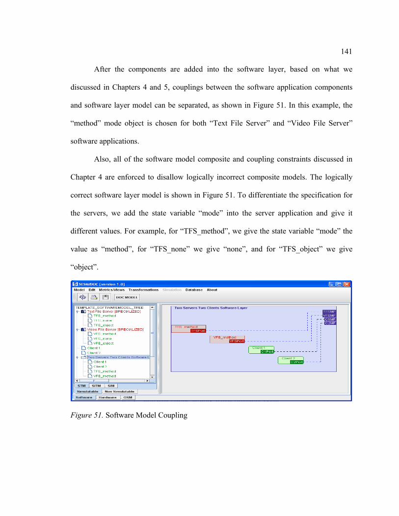
141
After the components are added into the software layer, based on what we
discussed in Chapters 4 and 5, couplings between the software application components
and software layer model can be separated, as shown in Figure 51. In this example, the
“method” mode object is chosen for both “Text File Server” and “Video File Server”
software applications.
Also, all of the software model composite and coupling constraints discussed in
Chapter 4 are enforced to disallow logically incorrect composite models. The logically
correct software layer model is shown in Figure 51. To differentiate the specification for
the servers, we add the state variable “mode” into the server application and give it
different values. For example, for “TFS_method”, we give the state variable “mode” the
value as “method”, for “TFS_none” we give “none”, and for “TFS_object” we give
“object”.
Figure 51. Software Model Coupling
142
6.2.4 Object System Mapping Design
In previous sections, we described how modelers use SESM/DOC to create
software and hardware models. In a distributed object computing system, the separation
is only one step of the system design. Another important step is object system mapping
That is, when one synthesizes the distinct software and hardware models. This synthesis
specifies a software layer model assignment to a hardware layer model.
In SESM/DOC, model synthesis happens in the OSM working section. The OSM
model creation is similar to hardware or software model creation except that the OSM
mode generation happens in the OSM working section and with the OSM model tree
structure. The unique part is adding components into the system model, and how to add
system mapping.
There are only two components in a system model – one software layer model and
one hardware layer model. These software layer and hardware layer models are not
generated in the OSM working section. In fact, they are generated in the DCO and LCN
working sections. As discussed in Chapter 5, the OSM integration can choose models in
the DCO and LCN tree structure to add into the OSM model. Figure 52 shows the co-
design model for the “H” style network model and Figure 53 shows the co-design for the
“I” style network model. The system model is the combination of the software, hardware,
and object system mapping models.

143
Figure 52. “H” Style OSM Model
Figure 53. “I” Style OSM Model
6.3 V&V Based on Model Types and Model Constraints
The model types and model constraints, defined in section 4.3, are helpful for to
the model design verification and validation. The modeler defines the constraints in an
effort to ensure the model relationships are correct. SESM/DOC uses these constraints to
provide help for verifying that the models generated are logically correct with respect to
the DOC abstract model.
In the search engine network example, each individual model is developed as a
particular model type. When the modeler attempts to created a relationship between
models (either a composite relationship or an assignment relationship), the relationship
144
must be verified to comply with the model constraints. Otherwise, the model design is
deemed incorrect regardless of the particular aspect of the system that is being modeled.
In Figure 40, the modeler adds components into a hardware group model, the
processor group. According to the model composite constraints, which state that a
processor group only contains processor models, the only model that can be added is the
SearchProcessor. If a router model is added, SESM/DOC provides an error message to
let the modeler know that this composition relationship is not valid. Although this is a
simple constraint, it is necessary to be enforced. It helps with the model verification and
validation process. Figure 42 shows five composite models (the “H” style hardware layer
model, the ProcGroup model, the NICGroup model, the LinkGroup model, and the
RouterGroup model). All of these composite models are valid since they satisfy the
model composite constraints.
The coupling relationships in this search engine network must also be verified
based on model coupling constraints. For example, in Figure 42, the ProcGroup model
needs to be coupled with the NICGroup model. If the ProcGroup is coupled with the
LinkGroup directly, such a coupling is invalid since the ProcGroup cannot be coupled
directly with a LinkGroup. In the same model, the NICGroup model plays an important
role by providing the media access control as discussed in Chapter 3. It must be inserted
between the PrcoGroup and LinkGroup. This application of model types and model
constraints aims to avoid some model design problems in a co-design network system.

145
6.4 Semi-automatic Simulation Code Generation
The SESM/DOC environment provides semi-automatic code generation using the
facilities provided by SESM. Both the XML code and the DEVS/DOC code can be semi-
automatically generated through a set of translators which query the information provided
by persistent models in the database. Since models for the software, hardware, and object
system models are needed, SESM/DOC provides separated name spaces (e.g.
directories). The software, the hardware, and the system model code are stored in
different directories. This allows the software, the hardware and the OSM models to have
identical names. For example, “File Server” can be the name of a software, a hardware,
or on OSM model. This naming convention avoids name collisions by providing different
name spaces for the models in different model layers. Tables 16 and 17 show the
generated XML file for “H” style hardware layer model, the DEVS/DOC code generated
for the network interface card (primitive model) and the “H” style network co-design
system model (composite model).
Table 16 Generated XML File
A piece of XML file for “H” style hardware layer model
<coupledModel name="H Style Hardware Layer_0"> <inport name="HLP1"> </inport> <inport name="HLP2"> …... <outport name="PGRP3"> </atomicModel> <atomicModel name="Processor_3">

146
<inport name="LPort"> </inport> <outport name="RPort"> </outport> </atomicModel> ……. <specialized name="NIC_1"> <atomicModel name="NIC_RBO_u"> ……..
Table 17 Generated DEVS/DOC Code
network interface card model
public class nic extends ViewableAtomic{ protected double processing_time; public nic(){this("nic", 0.0); } public nic(String name, double
processing_time){ super(name); ……….. addInport("in1"); addOutport("out1"); initialize(); } public void initialize(){ super.initialize(); phase = "passive"; sigma = INFINITY; } ……………… public message out(){ } ………
“H” style network co-design system model public class H Style Network Co-Design Model extends ViewableDiagraph{
public H Style Network Co-Design

147
Model(){ public H Style Network Co-Design
Model(String name){ super(name); ……… ViewableDiagraph Two Servers Two
Clients Software Layer_1 = new Two Servers Two Clients Software Layer();
ViewableDeagraph "H" Style Hardware Layer_1 = new "H" Style Hardware Layer();
add(Two Servers Two Clients
Software Layer_1); add("H" Style Hardware Layer_1); addCoupling(Two Servers Two
Clients Software Layer_1, "C1MP", "H" Style Hardware Layer_1, "HLP3");
.............
In SESM/DOC, the code generated for the primitive model is the partial code. It
contains the model’s input/output interface. The code generated for the composite model
represents all components and their relationships. Given the semi-automatically generated
code, code can be finished manually to produce the simulation models. Each of the
software, hardware, and OSM layer models, can be completed using non-visual tools
(e.g, Eclipse). The completed code can then be simulated in DEVS/DOC.
6.5 System Analysis
The system development includes both design and analysis. There can be multiple
model candidates. Each model candidate has its own software and hardware
topologies/configurations, assignment of software components to hardware components
given alternative aspects of a system, or level of detail contained in individual

148
components of the system model. One of the benefits of the separation of software and
hardware is that it is straightforward to consider how software or hardware affects one
another or the system model. In particular, simulation models can be generated,
simulated, and analyzed for purposes such as the performance modeling which is
described next.
6.5.1 System Simulation Experiments Set-Up
Each of the experiments provides a search engine application: the clients choose a
search key word and then make a search in the networks, the request will be routed to the
right server which provides the search service to the search request. To be a meaningful
computer network, it must have at least one server, one client, two processors, one link
and two network interfaces. OSM allows multiple software mappings to the same
hardware, so the possible experiments of software/hardware component ratios can be
found in the up-right zone within hardware/software boundaries, as shown in Figure 54.
In this section, five experiments are studied. The component configurations for the five
experiments are shown in Table 18. Based on the table below, the five experiments can
be traced in Figure 54.
Table 18 Experiments Settings
LCN Layer DCO Layer
component Processor Link Router Network interface sever client
OSM
Experiment1 10 2 1 10 2 8
Experiment2 10 5 2 10 2 8
Software for both servers and clients mapping to

149
Experiment3 16 15 0 16 1 15
Experiment4 16 15 0 16 1 15
Experiment5 3,…,103 1 0 3,…,103 1 2,…,999
processors
Figure 54. Experiments Boundary
In the following sections, the results of the five experiments are examined. The
first two experiments show how the change of hardware topology (with the same
software running inside) affects the system performance. The third experiment shows
how different software configurations in the same hardware topology affect the system’s
performance. The fourth experiment shows the performance changes due to the ad hoc
reconfiguration of the system. The last experiment addresses the scalability issue. All of
the experiments are done on a PC with a P4 3.2 GHz CPU, and 1 GB memory. Data are
collected based on 10 time runs of each simulation.
6.5.2 Alternative Hardware Network Analysis
As discussed above, manipulating hardware and software separately is one benefit
the modeler and the designer can get from SESM/DOC. In this chapter, two experiments
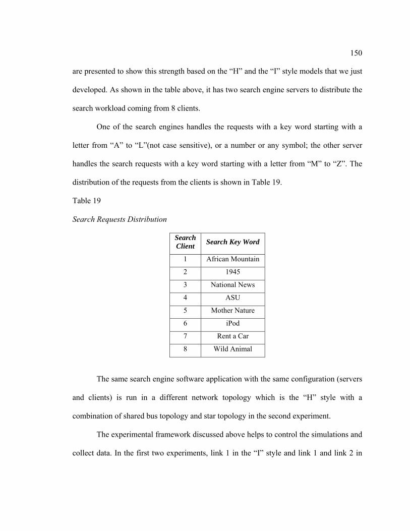
150
are presented to show this strength based on the “H” and the “I” style models that we just
developed. As shown in the table above, it has two search engine servers to distribute the
search workload coming from 8 clients.
One of the search engines handles the requests with a key word starting with a
letter from “A” to “L”(not case sensitive), or a number or any symbol; the other server
handles the search requests with a key word starting with a letter from “M” to “Z”. The
distribution of the requests from the clients is shown in Table 19.
Table 19
Search Requests Distribution
Search Client Search Key Word
1 African Mountain
2 1945
3 National News
4 ASU
5 Mother Nature
6 iPod
7 Rent a Car
8 Wild Animal
The same search engine software application with the same configuration (servers
and clients) is run in a different network topology which is the “H” style with a
combination of shared bus topology and star topology in the second experiment.
The experimental framework discussed above helps to control the simulations and
collect data. In the first two experiments, link 1 in the “I” style and link 1 and link 2 in

151
the “H” style are the objects to be studied. They are the links connected to the search
engine server and the behavior of these links is important to the performance of the whole
network.
From Figure 55 (a), the successful transmission in link 1 of the “I” style is equal
to the sum of the successful transmissions in link 1 and link 2 of the Hybrid Topology B.
This is due to an equal transmission load in these two networks. From Figure 55 (b) it can
be seen that, there are collisions in the “I” style but not in the “H” style. This is because
the traffic in the “H” style is distributed in different links, and the chance for the packets
to collide is much less than in the “I” style. This can also be obtained from the data in
sections (c) and (d) of the figure. The links’ Ethernet busy time is much shorter in the
“H” style than in the “I” style and the bandwidth utilization in the links of the “H” style is
also lower than in the “I” style. Figure 55 helps to arrive at the conclusion that by
distributing the network traffic, the “H” style gains shorter Ethernet busy time and much
less collisions than the “I” style, while at the same time sacrificing the lower bandwidth.
These comparisons are based on the same traffic load.

152
0
2
4
6
8
10
12
14
16
18
I H
succ
essf
ul tr
ansm
issi
on
Link 1
Link 2
Link 1
(a) successful transmission
0
2
4
6
8
10
12
I Link 1 H Link 1 H Link 2
colli
sion
num
ber
(b) collision number
0
0.005
0.01
0.015
0.02
0.025
I Link 1 H Link 1 H Link 2
ethe
rnet
bus
y tim
e
(c) ethernet busy time
0
10
20
30
40
50
60
70
80
I Link 1 H Link 1 H Link 2
band
wid
th u
tiliz
atio
n
(d) bandwidth utilization
Figure 55. Data Analysis for “I” Style and “H” Style
6.5.3 Alternative Software Network Analysis
With SESM/DOC, the hardware can be changed without any changes in the
software to achieve a different performance. Furthermore, the different software can be
exchanged to run on the same hardware to derive alternative system behaviors. In this

153
section, alternative software applications are simulated with a consistent hardware
topology.
In order to avoid the noise from unnecessary collisions and obtain more clear
data, a pure star network topology is chosen in experiment 3 to be the host where the
software applications can run as shown in Figure 56.
Figure 56. Star Network Topology
As discussed above, the software component in DEVS/DOC provides three
working modes: none, object, and method. In none mode, one software component can
only execute one job at a time and any additional requests are queued. It does not matter
how many methods the software component can provide, only one job can be executed at
one time. In object mode, one software component can have one job per defined method
concurrently active and, for the method mode, all the incoming requests can be executed
once they arrive at the hardware where the software is running. Returning back to the
search engine network example, the search engine software has up to three methods to

154
answer different search requests. Unlike the previous experiments, in experiment 3, the
search engine provides both the key word driven search, and the “key word plus format”
search. This can better help those clients who know more details about what they want by
providing more focused search results faster. In experiment 3, the server software
provides three methods to separate the request by the format they need. The first one is
for a text file, the second one is for a video file and the third one is for a binary file. The
15 clients in this experiment are divided into three groups and each has 5 clients. Each of
the three groups makes requests for a certain file format (text, video, and binary)
The server in experiment 3 handles the key word with the start letter from “A” to
“L” and any numbers and symbols. It also handles the three different file format requests
with three methods. The simulation runs 10 times for each software application mode.
As shown in Figure 57 (a) and (b), the work load in cpu during the 3 modes are
the same but they have a different multi-tasking degree due to their mode. This is because
in DEVS/DOC, a penalty mechanism is implemented in the object and method mode
which makes the object and method mode take a longer time to swap jobs in their multi-
tasking cpu. This mechanism leads to more CPU busy time as shown in Figure 57 (c),
with the same work load.
In the search engine example, one requirement is that the clients should get their
search results back in a similar time. Clients have no priority in the system. To be fair, the
response time should not vary too much. With 10 simulation runs for each of the three
modes; the max, min and average of the response time deviations are shown in Figure 57
(d). As discussed above, in none mode, only one job can be executed in a given time, the

155
other jobs have to wait. However, in object and method mode, multiple jobs can be
executed at the same time with a Round-Robin mechanism. This guarantees that all the
clients will be treated fair.
0
0.0001
0.0002
0.0003
0.0004
0.0005
0.0006
0.0007
0.0008
none object method
CPU
wor
k lo
ad
(a) CPU work load
0
2
4
6
8
10
12
14
16
none object method
degr
ee o
f mul
ti-ta
skin
g
(b) degree of multi-tasking
1.45
1.46
1.47
1.48
1.49
1.5
1.51
none object method
CPU
bus
y tim
e (s
econ
d)
(c) CPU busy time

156
(d) response time standard deviation
Figure 57. Data Analysis for Alternative Software Applications
6.6 Summary
This chapter considers search engine network systems and develops models of
these systems to illustrate how the co-design concepts, the model specifications, and the
approaches provided in Chapters 3, 4, and 5, work together to design a network system
model. These examples show that the co-design modeling approach enables the visual
design of network systems through the separation and synthesis of models from the
software/hardware model layers.
The examples show that the co-design persistent modeling approach makes the
SESM/DOC environment different from all other modeling and simulation environments
such as NS-2, OPNET, and TOSSIM, which store their models as files but not in the
database. Compared to SESM, SESM/DOC provides the capability to separate the model

157
repository for different model layers. The model types and the model constraints are
enforced in the SESM/DOC persistent modeling approach so that the visual modeling has
the syntax and semantic information. This persistent modeling approach provides help to
early stage model verification and validation which is based on these model types and
constraints. The use of the database also provides a measurement of the models structural
complexity.
Through the examples, it has been show that SESM/DOC provides flexibility for
modelers to consider the different software and hardware configurations and topologies.
This is due to the underlying SESM support for modeling families of models instead of
supporting the development of individual models. SESM/DOC extends this capability for
network co-design. The examples in Chapter 6 illustrate that the visual and persistent
approaches in SESM/DOC help the network systems co-design modeling. The modeler
can try different design options in the software and hardware models separately. This
separation is a big benefit due to the complexity of the distributed co-design network.
The partial co-design simulation code can be automatically generated and the structural
complexity of the network models can be calculated based on the software parts and
hardware parts.
7 CONCLUSION
7.1 A Comparison of SESM/DOC
This dissertation proposed a co-design modeling approach with a built-in
capability to visually develop models of network systems. To support model persistence,
the models are stored in a relational database. This approach has been prototyped and has
resulted in the SESM/DOC environment. In this section, the dissertation work is
examined in three parts. First, a selection of modeling and simulation approaches is
reviewed. Second, the SESM/DOC is compared with other approaches and tools that are
aimed at modeling and simulation of computer network systems. This entails some
informal considerations for using modeling tools. Finally, the role of the SESM/DOC in
supporting early-stage M&S verification and validation is briefly examined.
7.1.1 Modeling and Simulation Environments
To compare SESM/DOC, it is helpful to first consider modeling and simulation
approaches and environments that are not specialized for network systems. This
separation of modeling and simulation from one another is important in differentiating
visual model development and animation of simulation models. Table 21 is used to show
that different M&S approaches offer different types of support to the modelers and
simulationists (Sarjoughian, Fu, Bendre, & Flasher, 2007). The purpose of this table is
two-fold. First, it shows that modeling and simulation environments can be compared by
considering their capabilities along. Second, experiments (use-cases) may be developed
to assess the ‘operational’ aspects of these tools. For example, an approach and its tool
159
could be considered relatively simple for defining different kinds of models in a well
constrained domain from pre-built components. Another approach and tool, however,
could be difficult to use since models must be written in a programming language.
Clearly, developing a comprehensive evaluation across many modeling and
simulation tools both from capabilities and operational aspects is very important.
Undertaking such studies is outside the scope of this dissertation. Nonetheless, since
Table 20 compares SESM with a select group of other popular and influential modeling
and simulation tools, and that SESM/DOC is targeted for co-design modeling, we can
highlight some key differences between SESM/DOC and other approaches and
environments that are commonly used for modeling computer network systems.
Table 20. Comparison of selected general purpose modeling and simulation tools (Sarjoughian, Fu,
Bendre, & Flasher, 2007)
Modeling Simulation Tools Logical Visual Flat
Files Database Input/Output
Animation Run-time
Visual Trajectory Tracking
Formal Specification
DEVSJAVA Y N Y N Y N DEVS, OO Tracking Environment
Y N Y N N Y DEVS, OO
Ptolemy II Y Y Y N Y Y CSP, OO, CT, DE, DT
Simulink Y Y Y N Y Y Block models, OO
SESM Y Y Y Y N N System Theory, ER, OO, SES,
XML

160
A modeling engine supports the creation and edit of logical models by guiding
and enforcing structural and behavioral syntax and semantics of a modeling approach. It
provides specifications of models that can be simulated. A simulation engine is
responsible for executing the models that have well-defined specifications. For example,
an environment such as DEVSJAVA can be considered to be a simulation engine. This is
because this simulation engine is built to execute any model that is defined according to
the DEVS specification. For other tools such Ptolemy II (Eker, Janneck, Lee, Liu, Liu,
Ludvig, Neuendorffer, Sachs, & Xiong, 2003) and Simulink (Mathworks, 2007), it is
difficult to view them primarily as either a modeling or a simulation engine. SESM is a
modeling engine. This is because if we consider model development, then SESM offers
more capabilities since models have logical, visual, and persistent database schema
representations. On the other hand, if we consider domain-specific modeling, then
Simulink and Ptolemy II offer powerful pre-built models from which complex models
can be synthesized without much effort. Similarly, DEVSJAVA, Tracking Environment
(Singh & Sarjoughian, 2007), and Ptolemy II, for example, support animation.
For co-design modeling and simulation approaches and tools, SESM/DOC can be
used to describe a family of models with structures that conform to the DOC as well as
the SESM axioms. SESM/DOC is considered a modeling engine while DEVS/DOC is
considered primarily a simulation engine. The models created in a modeling engine need
to persist in some fashion. Some tools such as DEVSJAVA and NS-2 store their models
in flat files. The use of a database management system such as the one in SESM/DOC is
important when a family of alternative models must be developed and managed. A

161
database helps to manage a large number of models and it simplifies the measurement of
the structural complexity of the models.
7.1.2 Relating SESM/DOC with Other Network System Modeling
SESM/DOC extends SESM and emphasizes network systems co-design
modeling. Table 21 presents a comparison of SESM/DOC and other network system
modeling and simulation tools.
Table 21
Comparison of network system modeling and simulation tools
Co-design Modeling
Logical Visual Persistent
Simulation Formal Specification
DEVS/DOC Y N N Y DEVS, DOC, OO
DEVS-NS N N N Y DEVS, Queuing Theory, OO
NS-2 N N N Y Queuing Theory, OO OPNET N Y/N N Y Queuing Theory, OO SESM/DOC Y Y Y N Systems Theory, ER, OO,
SES, XML, DOC
From a co-design logical modeling point of view, both DEVS/DOC and
SESM/DOC are based on co-design logical modeling; others are not. DEVS-NS, NS-2,
and OPNET can be used to develop software or hardware models, but not in a systematic
way. The DOC abstract model in DEVS/DOC and SESM/DOC provide a set of well-
defined concepts for co-design logical modeling. For the visual modeling, DEVS/DOC,
DEVS-NS, and NS-2 provide a simulation view but not visual modeling. The model
design in these tools requires representing models in programming languages. OPNET is

162
marked as “Y/N” because although OPNENT supports visual models development, it
does not separate the software and hardware model design. Furthermore, a highly desired
capability for a visual modeling engine is to generate code that can be simulated with a
simulation engine. As a modeling engine, SESM/DOC can generate partial simulation
code. The partial simulation code must be completed using existing IDE tools before it
can be simulated in DEVS/DOC.
The latest version of the DESV/DOC environment is a portion of the work in this
dissertation. To compare DEVS/DOC with these tools for logical model design support,
the protocol stack plays an important role. All the computer networks modeling and
simulation environments provide facilities to implement the protocol stack
functionalities. Due to the critique of the description of the pure ISO/OSI model and
TCP/IP reference model, the hybrid reference model is used to present the protocol stack
of computer networks, as shown in Figure 58 (Tanenbaum, 1996).
Figure 58. Hybrid Reference Model for Computer Network Protocol Stack
A detailed study of approaches such as NS-2, GloMoSim, OPNET, and QualNet,
is provided in Chapter 2. These are compared in terms of the modeling which they

163
support for each network protocol stack layer. In Chapter 3, the DEVS/DOC
implementation details are provided. DEVS/DOC shows its strength for application layer
modeling with its specifications focusing on the separation and synthesis of
software/hardware co-design. In the application layer, DEVS/DOC provides a
computation unit for both software (DCO) and hardware (LCN) parts - the “swObject”
and the “processor” class. These allow the DEVS/DOC computation unit to have more
features in comparison with the node definition for NS-2, GloMoSim, and OPNET.
DEVS/DOC not only provides the generation of traffic (generating messages and jobs
through the network) but also has the facilities for processing the thread modes (i.e.,
none, object, and method) of software components. Supported by DCO (message and
pdu) and LCN (link, hub_ethernet, transport, and router) components, DEVS/DOC
provides multiple routing protocols and segment structures in the transport layer.
DEVS/DOC also provides unicast, broadcast and multicast in the network layer and the
media access control protocol in the link layer. In comparison, the NS-2 models are
detailed to capture realistic functionality of protocol stacks. The summary of the
discussion above and those presented in Chapters 2 and 3 is given in Table 22.
Table 22
Modeling and Simulation Supports in Network Protocol Layers
Hybrid Reference Model Layers Layer1 Layer2 Layer3 Layer4 Layer5
NS-2 Weak Support Strong Support GloMoSim Weak Support Strong Support OPNET Weak Support Strong Support QualNet Weak Support Strong Support TOSSIM No Support Strong Support No Support DEVS/DOC Strong Support Weak Support No Support

164
7.1.3 SESM/DOC and V&V
In Section 6.3, we discussed how the model types and model constraints can help
with model verification and validation in the search engine network example. A complete
study about the modeling verification and validation is beyond the scope of this
dissertation. Here we give a brief discussion about the role of SESM/DOC in supporting
early-stage M&S verification and validation. The SESM/DOC logical models are a set of
model types and model constraints for modeling the software and hardware layers of
network systems. The persistent modeling approach in SESM/DOC supports these model
types and constraints by saving the typing and constraints information in tables with
corresponding model identification. These constraints are important for validating user-
defined models. During model development, the modeler’s creation of models is enforced
to be consistent with the SESM/DOC approach. For example, an action to add a SMA
into a HLM will not be allowed based on the hardware layer model composite constraint
that HLM can only contain hardware models. Similarly, every coupling connection is
checked to be consistent with the allowed coupling types. For example, an action to
couple a PGM to a RGM would fail verification per the constraint that processors must
go through network interface cards and links to connect the routers.
By ensuring that only successfully verified composite and couplings constraints
exist, the modeler is provided some level of validation of the model. The logical, visual
and persistent modeling approaches with the model types and constraints for co-design
network systems enables the modeler to complement the syntax and semantics of the

165
modeling theory with the unique information that belongs to the co-design network
systems, and helps SESM/DOC support early-stage M&S verification and validation.
However, the V&V support is limited to the constraints that the modeler explicitly
specifies prior to model development. Validation of a system goes beyond model
composition and model coupling. It requires that the modeler understand the problem,
partitioned the problem appropriately, and incorporate capabilities into the models that
meet the needs of the modeled system. While the visual and persistent modeling in
SESM/DOC relieves the modelers from some basic steps in carrying out the verification
and validation processes, many other steps must be carried out with some combination of
other tools and techniques.
7.2 Summary
The widespread use of computer technology contributes to the complexity of
modern systems in part due to the ever increasing functionality of software components,
higher raw hardware computing and communication, and the multitude of ways software
and hardware components are integrated. An embedded system, which combines the
software and hardware components into one system, is a typical kind of system in which
software and hardware interact in complex ways to achieve their intended functionality.
Development of such systems poses a wide variety of challenges to designers. In
particular modelers need to develop software and hardware component models which
generally have mutually exclusive constraints and yet have to be integrated to satisfy
mixed system requirements.

166
Similarly, powered by the rapid advance of distributed computing, and network
technology, embedded systems are networked together more and more; creating
increasingly complex structures and behaviors. For network systems, it is useful to
separate the software components and hardware components for design and analysis
purposes. The combination of software and hardware, together with distributed
processing, make the distributed co-design network challenging to design and difficult to
analyze. As a result, we examined modeling of network system from a co-design
perspective where both the separation and the synthesis of software and hardware
components in order to make rigorous system model design is required and; therefore,
they have become very important in model driven engineering, and more specifically
simulation-based design.
There are many modeling and simulation approaches to help with the process of
large-scale and complex system design and analysis. Some of them are designed for
centralized embedded systems. However, few of modeling and simulation approaches
focus on decentralized or distributed co-design network systems. Most current modeling
and simulation approaches fall short of the requirements for presenting the software
aspects and hardware aspects of the system separately, satisfying software and hardware
requirements as well as the assignment of software components to hardware components
of networks systems. Satisfying separate and combined software and hardware layers of
system requirements is important for generating models that can be simulated.
This dissertation presented a co-design approach for developing models for the
software and hardware layers models of distributed systems. Based on a set of model

167
types, this modeling approach separates software and hardware models into their logical,
visual, and persistent models. For the logical model, this approach uses DOC abstract
models (DCO, LCN, and OSM) which are specified using the DEVS specification, to
define software model and hardware model. The logical constraints belonging to
software, hardware, and their mappings are incorporated into the SESM visual and
persistent modeling. The hierarchical component-based block and tree structure visual
modeling were developed to support the distinct DOC co-design requirements. The visual
model presents the components of the model and the relationship among models through
coupling and mapping. The visual model provides different levels of model
decomposition so that different aspects and resolution of model can be viewed. Three sets
of database schemas for the software model, the hardware model and the synthesized
system model are developed. The use of schemas ensures the systematic co-design for
network systems. The separated persistent model approach provides flexibility in the
sense that changes in software model data schema and changes in hardware model data
schema do not affect each other.
Based on the proposed approach, we have developed SESM/DOC, which is an
environment to support visual and persistent modeling for distributed network systems.
The environment is an extension of SESM. The logical, visual and persistent models in
SESM are extended to support the domain-specific model concepts (DCO, LCN, and
OSM) defined in DOC. The simulation model of DEVS/DOC can be partially generated
with the SESM/DOC. This relieves modelers from having to develop DEVS/DOC source

168
code from scratch. After the partial source code is completed, the simulation model can
be executed in the DEVS/DOC environment.
In SESM/DOC, models are divided into a software layer model, a hardware layer
model, and a system layer model. These different model layers are developed within their
own working sections and support modeling complex network systems. The visual
models for software and hardware are developed in a software model working section
and a hardware model working section separately. The system model is synthesized in the
system working section. This approach helps the modeler focus on what they want to
work on, either software models, hardware models, or the synthesized system model, and
not be interrupted by different model constraints from other model layers. In the system
model working sections, the system model is synthesized by mapping a chosen software
model from software model candidates in the software working section onto a chosen
hardware model from hardware model candidates in the hardware working section. In
both the software and hardware working sections, model decomposition and
specialization can be used to generate a model family for alternative system model
design. In the composite model and system mapping model, alternative system model
design can be realized by choosing a different specialized model from the same model
family. This distinguishes SESM/DOC from other modeling tools which lack a
framework to develop alternative model specifications in a disciplined fashion.
The software, hardware and synthesized system models that are designed in
separated working sections are each saved in their own database tables. The database
implementation enables the SESM/DOC environment to handle large-scale models. The

169
database records the modeling information in the logical model so that it can be used to
calculate the number of models, ports, and couplings. This provides an important
measurement of the system structural complexity.
With the ability to specify component-based models for a network system, the
SESM/DOC modeling approach has been developed based on the abstract distributed
object computing specification. Through the distributed co-design modeling example for
the searching engine network system, the software component model, the hardware
component model and the integrated system model are developed separately. Alternative
software models and alternative hardware models can be developed and chosen based on
a set of well-defined, general-purpose hierarchical (multi-resolution/multi-aspect)
modeling constraints, and can be synthesized as a different network system. The
SESM/DOC environment has been extended for the domain of network systems and
support modeling system networks that can be specified according to the DOC abstract
model and in particular models specified for simulation in DEVS/DOC. The structural
complexity metrics provided by the database can be used to evaluate the structural
complexity of network systems. The SESM/DOC approach is targeted for complex
systems (e.g., enterprise command and control) where key architectural decisions (e.g.,
service-oriented architecture)(Tsai, Chen, Paul, Zhou, & Fan, 2006) and computing
technologies (e.g., grid computing) are key for concept development and early design
stages.
As part of this dissertation and important for SESM/DOC, we also ported the
distributed object computing abstract models with DEVSJAVA 3.0 and JDK 1.5.
170
DEVSJAVA 3.0 and JDK 1.5 provide a new set of object collections and a user
interactive console for DEVS/DOC 2.0 simulation. This new DEVS/DOC
implementation is important because once the SESM/DOC partially generated simulation
code has been completed, the network system model can be simulated.
7.3 Future Works
SESM/DOC is the approach to develop distributed co-design models by
implementing multiple modeling layers in SESM. Since SESM/DOC supports
independent modeling of software, hardware, and system level modeling, it can be
extended with new model types, and therefore, offer additional modeling capabilities.
Multiple Domains Modeling and Simulation: For a Distributed Co-design
System: The SESM/DOC co-design modeling approach has been developed based on the
abstract distributed object computing specification. It provides partial code generation
based on the DEVS specification because DEVS/DOC is the implementation of the DOC
abstract model with DEVS specification. In the future, it is good to extend SESM/DOC
with other modeling and simulation specifications so that multiple domains modeling and
simulation approaches can integrate together for distributed co-design modeling. For
example, a set of discrete time specified software models may need to be mapped into a
set of discrete event specified hardware models to build a multiple domain distributed co-
design system.
Model Dynamic Properties Presentation: SESM/DOC provides the structure
properties for a distributed co-design system. It also has the facilities to add state

171
variables into software models and hardware models. In order to present the model’s
dynamic properties, the model state transaction needs to be addressed. In a distributed co-
design system, the software and hardware have different states and the state changes in
software components may or may not lead to the state change in hardware. Also, the state
changes in the hardware components may affect the state in the software components. To
give a complete set of state transactions for software and hardware components is good
for tracking the whole system’s state changes and for analyzing the dynamic properties of
the co-design system. Presenting model state transactions is also important for distributed
co-design modeling verification and validation in the sense of checking if the state
transaction leads the system to the correct state (Schulz, Rozenblit, & Buchenrieder,
2002).
Distributed Co-design Modeling Verification and Validation: SESM/DOC is well
suited for system architecture specifications. The separation of concern afforded by
SESM/DOC is important for model validation, verification, and accreditation (VV&A).
Since verification and validation is difficult for large-scale complex systems, the
disciplined approach supported by SESM/DOC provides a foundation for separating
software and hardware as well as synthesized system software/hardware VV&A. The
current SESM/DOC provides distributed co-design modeling constraints which are
helpful to V&V. It is not trivial and important in the future to provide more rigorous
semantics and syntax modeling verification and validation for distributed co-design
modeling. Model checking approaches will need to be added into SESM/DOC to
guarantee a models’ correctness.
172
Integration with Other Approaches: SESM/DOC provides visual and persistent
modeling for a distributed co-design system. It will be helpful for SESM/DOC to
integrate with other approaches such as IBM Eclipse and DEVS Simulation Tracking
Environment to get more facilities for modeling. Eclipse can provide a powerful
Integrated Development Environment (IDE) for the modeler to complete the partially
generated simulation code from SESM/DOC. The completed simulation code can be
compiled and run in Eclipse environment. Eclipse also provides numerous plug-ins which
may be used with SESM/DOC. DEVS Simulation Tracking Environment provides a
DEVS simulator and an analysis tool which tracks model state variable status for the
simulation model.

References:
Anand, S., Pandmanabhuni, S., & Ganesh, J. (2005). Perspectives on Service Oriented Architecture. IEEE International Conference on Services Computing, Orlando, FL, USA.
Arizona Center for Integrative Modeling and Simulation. (2007). "DEVSJAVA." 2007,
from http://www.acims.arizona.edu. Asimow, M. (1962). Introduction to Design, (1st. ed.), Prentice-Hall, 394. Bai, X. & Dey, S. (2001). High-Level Crosstalk Defect Simulation for System-On-Chip
Interconnects. 19th IEEE Proceedings on VLSI Test Symposium, Marina Del Rey, CA, USA.
Balci, O. (1997). Verification, Validation and Accreditation of Simulation Models. 1997
Winter Simulation Conference, Atlanta, GA, USA. Banks, J., Carson, J., Nelson, B., & Nicol, D. (2004). Discrete-Event System Simulation,
(4th. ed.), Prentice Hall, 624. Bendre, S. (2004). Behavioral Model Specification Towards Simulation Validation Using
Relational Databases. (Master Thesis, Arizona State University) Tempe, AZ. Bendre, S. & Sarjoughian, H. S. (2005). Discrete-Event Behavioral Modeling in SESM:
Software Design and Implementation. Advanced Simulation Technology Conf. San Diego, CA, USA.: 23-28.
Blanchard, B. S. (2004). System Engineering Management, (3rd. ed.), John Wiley &
Sons, Inc., 512. Brown, A. (2004). "An Introduction to Model Driven Architecture, Part I: MDA and
Today’s Systems." Retrieved Apr. 3rd, 2006, from http://www-128.ibm.com/developerworks/rational/library/3100.html.
Buede, D. M. (2000). The Engineering Design of Systems: Models and Methods, (1st.
ed.), John Wiley & Sons, 488. Burmester, S., Giese, H., & Henkler, S. (2005). Visual Model-Driven Development of
Software Intensive Systems: A Survey of Available Techniques and Tools. IEEE Symposium on Visual Languages and Human-Centric Computing, Dallas, Texas, USA.
Butler, J. M. (1995). Quantum Modeling of Distributed Object Computing. Simulation
Digest, 24(2), 20-39.
174
Chan, S. (2005). "Academic OPNET Research and Education Projects." Retrieved Nov.30, 2005, from http://proj.ee.cityu.edu.hk/opnet/Opnet.html.
Chapman, W. L., Bahill, A. T., & Wymore, A. W. (1992). Engineering Modeling and
Design, ed.) Boca Raton, FL, CRC Press, 400. Chapman, W. L., Rozenblit, J., & Bahill, A. T. (2001). System Design is an NP-Complete
Problem. System Engineering, 4(3), 222-229. Chen, P. (1976). The Entity-Relationship Model: Toward a Unified View of Data. ACM
Transactions on Database Systems, 1(1), 9-36. Cho, Y., Zeigler, B. P., Cho, H., & Sarjoughian, H. S. (2000). Design Considerations for
Distributed Real-Time DEVS. AI, Simulation and Planning, AIS2000. Tucson, Arizona, USA.
Chung, J. & Claypool, M. (2005). "NS by Example." Retrieved Nov. 25, 2006, from
http://nile.wpi.edu/NS/. Clayberg, E. & Rubel, D. (2006). Eclipse: Building Commercial-Quality Plug-ins, (2nd.
ed.), Addison-Wesley Professional, 810. Cyberspace Center. (1997). "Introduction to Intranet Technologies and Products." 2006,
from http://www.cyber.ust.hk/handbook3/hb3main.html. Dai, H., C. & Scott, K. (1995). AVAT, A CASE Tool For Software Verification and
Validation. IEEE Seventh International Workshop on Computer-Aided Software Engineering. Toronto, Ontario, Canada.
Davis, P. K. & Anderson, R. H. (2004). Improving the Composability of DoD Models
and Simulations. JDMS: the Journal of Defense Modeling and Simulation: Applications, Methodology, Technology, 1(1), 5-17.
Eker, J., Janneck, W., Lee, E. A., Liu, J., Liu, X., Ludvig, J., Neuendorffer, S., Sachs, S.,
& Xiong, Y. (2003). Taming Heterogeneity--the Ptolemy Approach. Proceedings of the IEEE, 91(2), 127-144.
Elamvazhuthi, V., Sarjoughian, H. S., & Hu, W. (2007). UML Database Specification for
SESM. Internal Report, ACIMS, Arizona State University. Erdogan, S., McFarr, S., & Maglidt, D. (1989). EDEN: An Integrated Computer-Aided
Software Engineering Environment. IEEE Eight Annual International Conference on Computers and Communications. Phoenix, AZ, USA.

175
Fall, K. & Kannan, V. (2005). "The NS Manual." Retrieved Nov. 27, 2006, from http://www.isis.edu/nsnam/ns//doc/ns_doc.pdf.
Ferayorni, A. & Sarjoughian, H. S. (2007). Domain Driven Modeling for Simulation of
Software Architectures. Summer Computer Simulation Conference, San Diego, CA, USA.
Fishwick, P. A. (1995). Simulation Model Design and Execution: Building Digital
Worlds, (1st. ed.), Prentice Hall, 432. Frankel, D. S. (2003). Model Driven Architecture: Applying MDA to Enterprise
Computing, (1st. ed.), Wiley Publishing, Inc., 352. Fu, T. (2002). Hierarchical Modeling of Large-Scale Systems Using Relational
Databases. (Master Thesis, University of Arizona) Tucson, AZ. Fujimoto, R. (2000). Parallel and Distributed Simulation Systems, (1st. ed.),
Wiley_Interscience, 320. Gamma, E., Helm, R., Johnson, R., & Vissides, J. (1995). Design Patterns: Elements of
Reusable Object-Oriented Software, (1st. ed.), Addison-Wesley, 416. Gerla, M. B., R., Zhang, L., Tang, K., & Wang, L. (1999). TCP Over Wireless Multihop
Protocols: Simulation and Experiments. IEEE International Conference on Communications, Jaipur, India.
Gery, E., Harel, D., & Palachi, E. (2002). Phapsody: A Complete Life-Cycle Model-
Based Development System. The Third International Conference on Integrated Formal Methods, Turku, Finland.
Global Mobile Information Systems Simulation Library. (2005). "GloMoSim."
Retrieved March, 2005, from http://pcl.cs.ucla.edu/projects/glomosim. Godding, G., Sarjoughian, H. S., & Kempf, K. (2007). Application of Combined
Discrete-Event Simulation and Optimization Models in Semiconductor Enterprise Manufacturing Systems. Winter Simulation Conference, Washington D.C. USA.
Gokhale, A., Batarajan, B., Schmidt, D. C., & Wang, N. (2002). Applying Model-
Integrated Computing to Component Middleware and Enterprise Application. ACM Special Issue on Enterprise Components, Services and Business Rules.
Graaf, B., Lormans, M., & Toetenel, H. (2003). Embedded Software Engineering: The
State of The Practice. IEEE Software, 20(6), 61-69.

176
Harel, D. (1987). Statecharts: A Visual Formalism for Complex Systems. Science of Computer Programming Archive, 8(3), 231-274.
Hause, M., Thom, F., & Moore, A. (2005). Inside SysML. Computing and Control
Engineering Journal, 16(4), 10-15. Herzen, V. & Lerer, M. (2006). Grand Challenge: The Future of CMOS System-on-Chip
Hardware and Software Application Development. IEEE Workshop on Design, Application, Integration and Software, Dallas, TX, USA.
Higham, D. J. & Higham, N. J. (2000). MATLAB Guide, (1st. ed.) Philadelphia, Society
for Industrial and Applied Mathematics, 382. Highland System Inc. (2005). "Bluetooth Simulation Model Suitable for OPNET."
Retrieved Dec. 20, 2006, from http://www.highsys.com/products/Suiteooth.pdf. Hild, D. R. (2000). DEVS-Based Co-Design Modeling and Simulation Framework and Its
Supporting Environment. (Ph.D Dissertation, University of Arizona) Tucson, AZ. Hild, D. R., Sarjoughian, H. S., & Zeigler, B. P. (2002). DEVS-DOC: A Modeling and
Simulation Environment Enabling Distributed Codesign. IEEE SMC Transactions, 32(1), 78-92.
Hu, W. & Sarjoughian, H. S. (2005). Discrete-Event Simulation of Network Systems
Using Distributed Object Computing. International Symposium on Performance Evaluation of Computer and Telecommunication Systems, Philadelphia, PA, USA.
Hu, X. & Zeigler, B. P. (2005). Model Continuity in the Design of Dynamic Distributed
Real-Time Systems. IEEE Transactions on Systems, Man and Cybernetics, 35(6), 867-878.
Hwang, M. H. & Zeigler, B. P. (2006). A Modular Verification Framework using Finite
and Deterministic DEVS. 2006 DEVS Integrative M&S Symposium, Huntsville, AL, USA.
IEEE (1993). IEEE Standards Collection: Software Engineering. 610.12-1990. Information Sciences Institute. (2004). "The Network Simulator - ns-2." Retrieved
March, 2006, from http://www.isi.edu/nsnam/ns. Institute of Electrical and Electronics Engineers (2000). IEEE Standard for Modeling and
Simulation (M&S) High Level Architecture (HLA)-Object Model Template (OMT) Specification. IEEE Std 1516.

177
Institute of Electrical and Electronics Engineers (2000). IEEE Standard for Modeling and Simulation (M&S) High Level Architecture (HLA) - Framework and Rules. IEEE Std 1516-2000.
Jaikaeo, C. & Shen, C. (2005). "QualNet Tutorial." Retrieved Jan. 6, 2006, from
http://www.it.iitb.ac.in/~it601/resources/simulator_workshop/QualNet-Tutorial.pdf.
Johnson, M. & Mckeon, M. (1998). SBA: Simulation Based Acquisition: A New
Approach. Report of the Military Research Fellows DSMC, Technical Report, Defense System Management College.
Karris, S. (2006). Introduction to Simulink with Engineering Applications, (1st. ed.),
Orchard Publication, 584. Klir, G. J. (1985). Architecture of Systems Complexity, (1st. ed.) New York, Sauders,
238. Kofman, E., Lapadula, M., & Pagliero, E. (2003). "PowerDEVS: A DEVS–Based
Environment for Hybrid System Modeling and Simulation." Retrieved May 30, 2007, from http://www.fceia.unr.edu.ar/~kofman/files/lsd0306.pdf.
Krishnakumar, B., Gokhale, A., & Karsai, G. (2006). Developing Applications Using
Model-Driven Design Environments. IEEE, Computer,(2), 33-40. Lee, E. A. (2000). What's Ahead of Embedded Software. IEEE Computer, 9(33), 18-26. Levis, P. & Lee, N. (2003). "TOSSIM: A Simulator for TinyOS Networks." Retrieved
Jan.5, 2007, from http://www.cs.berkeley.edu/~pal/pubs/nido.pdf. Levis, P., Lee, N., Welsh, M., & Culler, D. (2003). TOSSIM: Accurate and Scalable
Simulation of Entire TinyOS Applications. Proceedings of the First ACM Conference on Embedded Networked Sensor Systems, Los Angeles, CA, USA.
Lunceford, D. (2002). State of SMART. Simulation and Modeling for Acquisitions,
Requirements, and Training Conference, Salt Lake City, UT, USA. Mathworks. (2007). "MATLAB/SIMULINK." 2007, from http://www.mathworks.com/. McDermid, J. & Rook, P. (1993). Software Development Process Models. Software
Engineering's Reference Book, CRC Press: 103-248.

178
Microsoft. (2006). "Net Framework." Retrieved Apr. 4, 2007, from http://msdn2.microsoft.com/en-us/netframework/default.aspx.
Mohan, S. (2003). Measuring Structural Complexities of Modular, Hierarchical Large-
scale Models. (Master Thesis, Arizona State University) Tempe, AZ. Muth, T. G. (2005). Functional Structures in Networks: AMLn - A Language for Model
Driven Development of Telecom Systems, (1st. ed.) New York, Springer Berlin Heidelberg, 280.
National Research Council (2002). Modeling and Simulation in Manufacturing and
Defense Acquisition: Pathways to Success. National Academy Press. Nutaro, J. & Hammonds, P. (2004). Combining the Model/View/Control Design Pattern
with the DEVS Formalism to Achieve Rigor and Reusability in Distributed Simulation. JDMS: The Journal of Defense Modeling and Simulation: Applications, Methodology, Technology, 1(1).
Object Management Group. (2005). "CORBA Basics." Retrieved Nov. 11th, 2005, from
http://www.omg.org/gettingstarted /corbafaq.htm. Object Management Group. (2007). "UML Resource Page." Retrieved July 2, 2007,
from http://www.uml.org/. Olson, J., Rozenblit, J., & Jacak, W. (2007). Hardware/Software Partitioning using
Bayesianbelief Networks. IEEE Transactions on Systems, Man and Cybernetics, in print.
OPNET Technologies. (2004). "OPNET Modeler." Retrieved Dec. 12th, 2006, from
http://www.opnet.com. Park, S., Zeigler, B. P., & Sarjoughian, H. S. (2001). Interface for Scalable DEVS and
Distributed Container Object Specifications. IEEE Sys. Man. Cyber. Conference. Tuscon, AZ, USA.: 93-98.
Park, S., Zeigler, B. P., & Sarjoughian, H. S. (2001). Interface for Scaleable DEVS and
Distributed Container Object Specifications. Systems, Man, and Cybernetics, Tucson, AZ.
Pei, G. (1997). "GlomoSim Simulation Layers." Retrieved Nov. 27, 2006, from
http://pcl.cs.ucla.edu/slides/api.

179
Pressman, R. S. (2005). Software Engineering: A Practitioner's Approach, (6th. ed.), McGraw-Hill, 880.
Pressman, R. S. (2005). Software Engineering: A Practitioner's Approach, (6. ed.),
McGraw-Hill, Riley, G. F. & Ammar, M. H. (2002). Simulating Large Networks - How Big is Big
Enough. International Conference on Grand Challenges for Modeling and Simulation, San Antonio, Texas, USA.
Rozenblit, J. & Buchenrieder, K. (1995). Codesign: Computer-aided Software/Hardware
Engineering, (1st. ed.), IEEE, 464. Rutherford, M. J. & Wolf, A. L. (2003). A Case for Test-Code Generation in Model-
Driven Systems. Proceedings of The Second International Conference on Generative Programming and Component Engineering GPCE, Erfurt, Germany.
Sage, A. P. & Armstrong, J. E. J. (2000). Introduction to Systems Engineering, (1st. ed.),
John Wiley & Sons, Inc., 568. Sargent, R. G. (2000). Verification, Validation and Accreditation of Simulation Models.
Proceeding of the 2000 Winter Simulation Conference, Orlando, FL, USA. Sarjoughian, H. S. (2001). An Approach for Scaleable Model Representation and
Management. Internal Report, Arizona State University. Sarjoughian, H. S. (2005). A Scalable Component-based Modeling Environment
Supporting Model Validation. Interserive/Industry Training, Simulation, and Education Conference, Orlando, FL, USA.
Sarjoughian, H. S. & Cellier, F. (2001). Discrete Event Modeling and Simulation
Technologies: A Tapestry of Systems and AI-Based Theories adn Methodologies, (1st. ed.) New York, Springer Verlag, 1-12.
Sarjoughian, H. S., Fu, T.-S., Bendre, S., & Flasher, R. (2007). A Unified Logical, Visual,
and Persistent Modeling Framework. Working Paper, Computer Science and Engineering Dept. Arizona State University, Tempe, AZ, USA.
Sarjoughian, H. S., Hild, D. R., & Zeigler, B. P. (2000). DEVS-DOC: A Co-Design
Modeling and Simulation Environment. IEEE Computer, 3(33), 110-113.

180
Sarjoughian, H. S., R. Flasher (2007). System Modeling with Mixed Object and Data Models. DEVS Symposium, Spring Simulation Multi-conference, Norfolk, VA, USA.
Sarjoughian, H. S. & Singh, R. K. (2004). Building Simulation Modeling Environments
Using Systems Theory and Software Architecture Principles. Advanced Simulation Technology Symposium (ASTC), Washington D.C., USA.
Schilesinger, S. (1979). Terminology For Model Credibility. Simulation, 32(3), 103-104. Schmidt, D. C. (2006). Model-Driven Engineering. IEEE, Computer, 39(2), 25-31. Schulz, S., Rozenblit, J., & Buchenrieder, K. (2002). Multi-Level Testing for Design
Verification of Embedded Systems. IEEE Design and Test. 19: 60-69. SEI. (2000). "SEI Open Systems Glossary." Retrieved May 10th, 2006, from
http://www.sei.cmu.edu/opensystems/glossary.html. Seo, S.-H., Lee, S.-W., Hwang, S.-H., & Jeon, J. W. (2006). Development of Platform for
Rapid Control Prototyping Technique. SICE-ICASE International Joint Conference, Busan, Korea.
Shaukat, K. & Sarjoughian, H. S. (2007). A Comparison Between DEVS and NS-2.
Internal report, ACIMS, Arizona State University. Shaw, M. & Garlan, D. (1996). Software Architecture, (1st. ed.), Prentice-Hall, 361. Singh, R. K. & Sarjoughian, H. S. (2007). Software Architecture for Object-Oriented
Simulation Modeling and Simulation Environments: Case Study and Approach. Technical Report. TR-03-09, Department of Computer Science and Engineering, Arizona State Univeristy, Tempe, AZ, USA.
Skyttner, L. (2001). General System Theory: Ideas and Applications, (1st. ed.), World
Scientific Publishing, 459. Stephens, R. & Plew, R. (2006). "Logical Versus Physical Database Modeling."
Retrieved Mar. 10th, 2006, from http://www.developer.com/tech/article.php/641521.
SUN. (2005). "JavaTM 2 Platform Standard Edition 5.0, API Specification." from
http://java.sun.com/j2se/1.5.0/docs/api/index.html. Tanenbaum, A. S. (1996). Computer Networks, (3rd. ed.), Prentice Hall, 912.

181
Tsai, W. T., Chen, Y., Paul, R., Zhou, X., & Fan, C. (2006). Simulation Verification and Validation By Dynamic Policy Specification and Enforcement. Simulation, Transactions of the Society for Modeling and Simulation International, 82(5), 295-310.
Wasson, C. S. (2006). System Analysis, Design, and Development: Concepts, Principles,
and Practices, (1st. ed.), Wiley-Interscience, 818. World Wide Web Consortium. (1998). "Extensible Markup language (XML)." Retrieved
May 25, 2007, from http://www.w3.org/XML/. Wymore, A. W. (1993). Model-Based Systems Engineering, (1st. ed.) Boca Raton, FL:
736. Xie, B. (2004). Development of Model Component Templates for Semiconductor
Manufacturing Process Simulation in DEVSJAVA. (Master of Computer Science Project, Arizona State University) Tempe, AZ.
Young, M., Cook, J., & Mahabadi, L. (2003). "Stochastic Local Search Algorithms for
Minimizing Edge Crossings in Complete Rectilinear Graphs." Retrieved Jun. 7, 2006, from http://www.cs.unm.edu/~young/final_report.pdf.
Zeigler, B. P., Praehofer, H., & Kim, T. G. (2000). Theory of Modeling and Simulation,
(2nd. ed.), New York: Academic, 510. Zeigler, B. P. & Sarjoughian, H. S. (2002). Implications of M&S Foundations for the
V&V Large Scale Complex Simulation Models. Foundations for the V&V in the 21st Century Workshop (Foundations '02). San Diego, CA, USA. From https://www.dmso.mil/public/library/projects/vva/found_02/sess_papers/a6.pdf.
Zhong, L., Rabaey, J., Guo, C., & Shah, R. (2001). Data Link Layer Design for Wireless
Sensor Networks. IEEE Communications for Network-Centric Operations, Mclean, VA, USA.


![partial] fulfillment Town](https://img.pdfslide.net/doc/110x75/61cbd0e20c1fcf7e016f4ea2/partial-fulfillment-town.jpg)