Embed Size (px)
Citation preview
A Dissimilarity Measure for Comparing Origami Crease Patterns
Seung Man Oh1, Godfried T. Toussaint1, Erik D. Demaine2 and Martin L. Demaine2
1Department of Computer Science, New York University Abu Dhabi, Saadiyat Island, UAE2Computer Science and Artificial Intelligence Laboratory, MIT, Cambridge, USA
[email protected], [email protected], [email protected], [email protected]
Keywords: Computational Origami, Graph Similarity, Geometric Graphs, Crease Patterns, Phylogenetic Trees
Abstract: A measure of dissimilarity (distance) is proposed for comparing origami crease patterns represented as ge-ometric graphs. The distance measure is determined by minimum-weight matchings calculated between theedges as well as the vertices of the graphs being compared. The distances between pairs of edges and pairsof vertices of the graph are weighted linear combinations of six parameters that constitute geometric featuresof the edges and vertices. The results of a preliminary study performed with a collection of 45 crease pat-terns obtained from Mitani’s ORIPA web page, revealed which of these features appear to be more salient forobtaining a clustering of the crease patterns that appears to agree with human intuition.
1 Introduction
The origin of the art of paper folding, known aszhezhi in China and origami in Japan is not certain,but the modern Japanese art known as Origamitraces its roots to somewhere around the 9th century(Demaine and O’Rourke, 2007), (McArthur andLang, 2013). Origami differs from other currentpaper art in that the final object is typically madepurely by folding the paper without cutting, stretch-ing, or otherwise damaging it. From its originsas a purely aesthetic game, origami evolved togain practical and theoretical significance in the20th century, as its rules were discovered and themathematical principles that govern it began to beunderstood (Lang, 1996), (Bern and Hayes, 1996),(Demaine and Demaine, 2001), (O’Rourke, 2011).Computational origami finds application today ina wide variety of endeavors including architecture(Tachi, 2010), (Liapi, 2002), pop-up books and cards(O’Rourke, 2011), folding rigid materials (Balkomet al., 2004), (Wu and You, 2011), and map folding(Arkin et al., 2004). Origami is ideally suited forsolving the problem of packaging large objectsinto a small volume, such as designing airbags forcars, creating foldable heart stints (that need toinflate once they arrive at their destination to keeparteries open in heart-attack patients), and in folding100-meter diameter telescopes into three meter boxesfor a spacecraft to deliver to outer space (Lang, 1996).
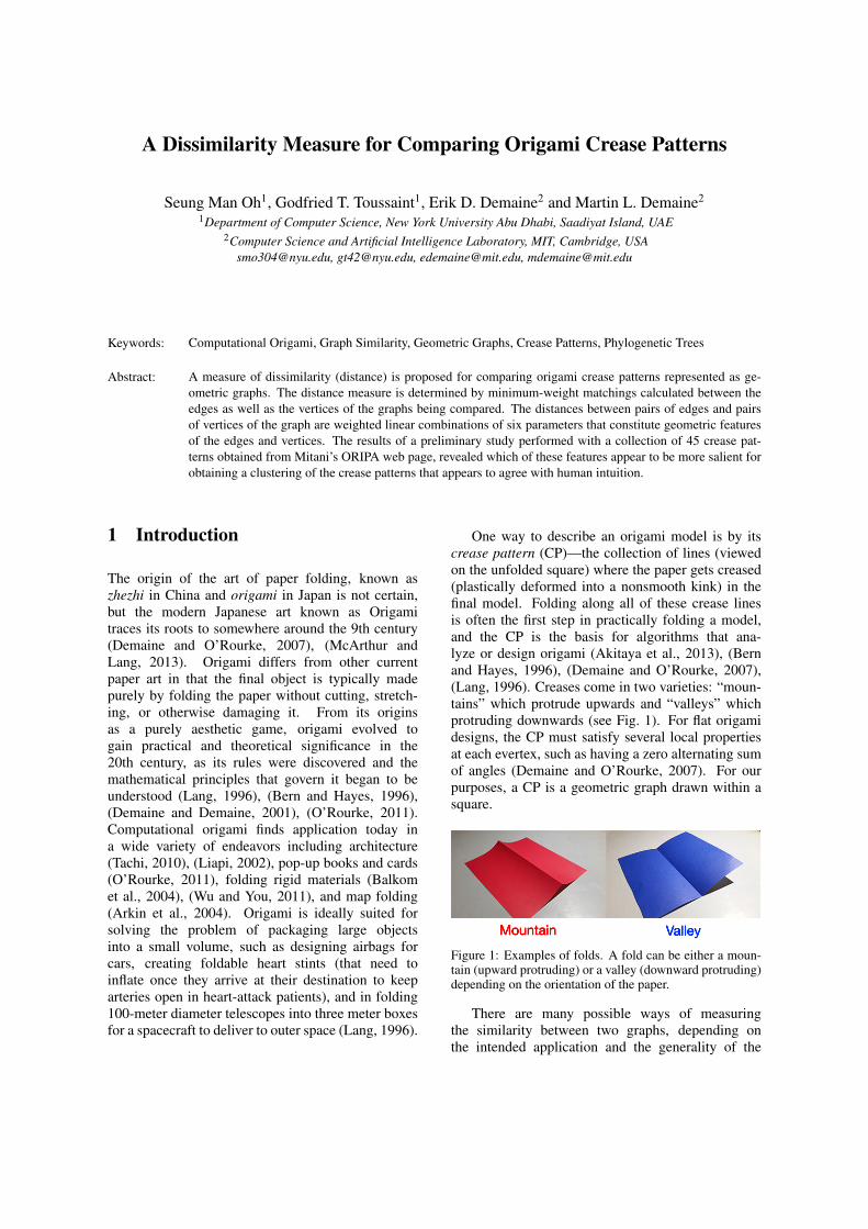
One way to describe an origami model is by itscrease pattern (CP)—the collection of lines (viewedon the unfolded square) where the paper gets creased(plastically deformed into a nonsmooth kink) in thefinal model. Folding along all of these crease linesis often the first step in practically folding a model,and the CP is the basis for algorithms that ana-lyze or design origami (Akitaya et al., 2013), (Bernand Hayes, 1996), (Demaine and O’Rourke, 2007),(Lang, 1996). Creases come in two varieties: “moun-tains” which protrude upwards and “valleys” whichprotruding downwards (see Fig. 1). For flat origamidesigns, the CP must satisfy several local propertiesat each evertex, such as having a zero alternating sumof angles (Demaine and O’Rourke, 2007). For ourpurposes, a CP is a geometric graph drawn within asquare.
Mountain Valley
Figure 1: Examples of folds. A fold can be either a moun-tain (upward protruding) or a valley (downward protruding)depending on the orientation of the paper.
There are many possible ways of measuringthe similarity between two graphs, depending onthe intended application and the generality of the
class of graphs considered. Origami crease pat-terns belong to the class of geometric graphs inwhich the locations of the vertices are fixed andspecified by their x and y coordinates, and theedges connecting pairs of vertices are straight lines(Pach, 2004). Similarity (distance) measures ingeometric graphs generally can be divided into twoapproaches: syntactic, where the graph is divided upinto geometric “features” whose relative positionsare then compared, or earth-movers distance methods(transformation or edit methods) which measure howmuch one graph needs to be changed in order tobe transformed into the other graph (Gao et al., 2010).
Gu and Guibas defined a distance functionbetween two flat-folded 1D folds as a “distanceroot mean squared error” (dRMS) metric, whichcalculates the distances between each internal pointwith every other internal point (Gu and Guibas,2011). Experiments with 40 random folding patternsconfirmed a clustering of similar patterns. Unfortu-nately this method does not generalize to 2D foldsthat contain non-horizontal or non-vertical edges. Foractual origami pieces, which can be realized in 3D or2D with internal structure, direct comparison of thefolded objects is difficult. Ronald Graham describesan idea for which he credits Stan Ulam, suggestingthat the similarity of two graphs could be measuredby decomposing the graphs into a number of pairwiseidentical subgraphs, so that the smaller the numberof subgraphs needed, the more similar are the graphs(Graham, 1987). This is an interesting approach thatapplies to very general graphs, and which has notbeen explored in practical situations, but is difficultto compute. In a dimensionality reduction approachRobles-Kelly and Hancock convert a two dimensionalgraph into a one-dimensional string, and then applythe well known edit (or Levenshtein) distance (Postand Toussaint, 2011), (Levenshtein, 1966) betweenstrings to measure the distance between the originalgraphs (Robles-Kelly and Hancock, 2005).
In a variant of the approach taken by Graham(Graham, 1987), Fei and Huan introduce a methodbased on subgraph selection (Fei and Huan, 2008).The subgraphs that appear most frequently arechosen as features, and their frequency and spatialrelationship are used to rank each subgraph. This“structure based feature selection method” was testedon several datasets of graphs that describe chemicalstructures, and was found to outperform several otherfeature selection methods.
Cheong et al. proposed a geometric graph dis-
tance that is a slight variation of the edit distance tomake it work optimally for geometric graphs ratherthan arbitrary graphs (Cheong et al., 2009) . Thisis achieved by taking into account the order of thesequence needed for performing the edits. Theirpaper assumes translations, rotations, and scaledgraphs to be dissimilar, making it unsuitable forcomparing CPs.
When the graphs being compared have the samenumber of elements, a natural approach to mea-sure their similarity is via a minimum cost perfectmatching between their elements. However, inmany applications in the real world the graphs beingcompared have unequal numbers of features, as is thecase with origami crease patterns. One approach tohandling such general situations has been to merge(or split) vertices and edges so as to make the twographs have the same number of elements, and sub-sequently apply one-to-one matching (Berretti et al.,2004), (Ambauen et al., 2003). Such an approachmakes sense in certain computer vision applications,but not for matching CPs in origami.
Here we propose a conceptually simple geomet-ric distance measure constructed from two completebipartite graphs defined between the edges (edge toedge) and nodes (vertex to vertex), respectively, of thetwo graphs being compared. In each bipartite graphthe minimum-weight perfect matching is calculated,and their costs added. The weights between pairs ofedges and pairs of vertices of the graph are weightedlinear combinations of simple geometric features ofthe edges and vertices of the crease patterns. Wepresent and discuss the results of a preliminary studyperformed with the Hungarian algorithm on a col-lection of 45 crease patterns obtained from Mitani’sORIPA web page. Using phylogenetic techniques weuncover which of these geometric features appear tobe more salient for obtaining a clustering of the creasepatterns that appears to agree with human intuition.We also suggest avenues for further research.
2 Methodology
2.1 ORIPA Dataset
An origami crease pattern database was downloadedfrom Mitani’s ORIPA homepage (Mitani, 2011). Thedataset consists of a total of 47 patterns in Oripaformat, an XML-like format that stores informationabout the edge type (mountain or valley) and the xand y coordinates of the two endpoints of every edge.
Two of the patterns were examples of bad creasepatterns, so were excluded from testing. Four pairs ofpatterns that were deemed similar were selected fora preliminary pilot study in order to test the efficacyof the procedure before using larger datasets. Byconvention, the coordinates range from -200 to 200.Since the four boundary lines of the square pieceof paper are common to all the crease patterns theydo not constitute either a mountain or a valley, andwere omitted from the graph descriptions. Similarly,“guideline” edges (shown as green dotted lines) thatare used to help the folding process were omitted asthey are not required for the actual construction ofthe final folded objects.
2.2 Dissimilarity Metric
Let CP1 and CP2 be two crease patterns (representedas geometric graphs) that are to be compared accord-ing to their dissimilarity or distance from each other.The proposed distance measure between the twocrease patterns is defined as the cost of a minimum-weight perfect matching in a complete bipartite graphK(CP1,CP2) that connects with an arc every elementof CP1 with every element of CP2. The links connect-ing two vertices in a graph are usually called eitherarcs or edges. Here we reserve the term arc for thelinks in the bipartite graphs linking the two CPs, andthe term edges for the links of the vertices in the CPs,to avoid confusion. Since the CPs are made up oftwo types of elements, namely vertices (points) andedges (creases), and these geometric objects are quitedifferent from each other, it is convenient to first com-pute the two matchings separately, and subsequentlyto add their costs together. Thus two complete bipar-tite graphs are first computed, one for matching theedges of the CPs denoted by KE(CP1,CP2), and thesecond for matching the vertices of the CPs denotedby KV (CP1,CP2). The weights of the arcs of bothbipartite graphs are linear functions of the geometricfeatures calculated from the edges and the vertices ofthe CPs. More specifically, the weight of an arc inKE(CP1,CP2) that connects some edge ε1 in CP1 withsome edge ε2 in CP2 is defined as a linear combinationof the following four features: e1 denotes the differ-ence between the lengths of ε1 and ε2, e2 is the smallerof the two angles between the lines containing ε1 andε2, e3 is the minimum Euclidean distance between apoint in ε1 and a point in ε2, and e4 indicates the edgetype (mountain or valley). Each of these features is
normalized to 1 as follows:E1 = (e1)/
√2 (1)
E2 = (e2)/2π (2)
E3 = (e3)/√
2 (3)E4 = (e4) (4)
The weight of an arc in KV (CP1,CP2) that connects avertex ω1 in CP1 with a vertex ω2 in CP2 is definedas a linear combination of the following two features:v1 denotes the difference in the degrees of ω1 and ω2,and v2 stands for the Euclidean distance between ω1and ω2. Similar to the edge distance, v2 was nor-malized by dividing by
√2. The vertex degrees were
more problematic to normalize than the distances be-cause their values ranged from 0 to more than 30, withno noteworthy distribution. However, since prelimi-nary testing with the pilot dataset showed that v1 wasa poor indicator of geometric graph dissimilarity, itwas given a negligible weight. The two normalizedfeatures are given by:
V1 = (v1) (5)
V2 = (v2)/√
2 (6)The above features for comparing the edges and ver-tices of a pair of CPs, determine the weights of thearcs in the complete bipartite graph KE(CP1,CP2).For an edge ε1 in CP1, and an edge ε2 in CP2, denotethe weight of the arc in KE(CP1,CP2) which connectsε1 and ε2 by dE(ε1,ε2). Then this weight is given bythe equation:
dE(ε1,ε2) =4
∑i=1
weiEi (7)
These weights are used to compute the minimum-weight matching in KE(CP1,CP2). Let the resultingcost be CE(CP1,CP2).
Similarly, for a vertex ω1 in CP1, and a vertex ω2in CP2, denote the weight of the arc in KV (CP1,CP2)which connects ω1 and ω2 by dV (ω1,ω2). Then thisweight is given by the equation:
dV (ω1,ω2) =2
∑j=1
wv jVi (8)
These weights are used to compute the minimum-weight matching in KV (CP1,CP2), with resulting costCV (CP1,CP2).
Finally, the overall distance (cost) between CP1 andCP2 is defined as:
D(CP1,CP2) =CE(CP1,CP2)+CV (CP1,CP2). (9)Note that the wei and wv j in the above equations areadditional weights that can be tuned so as to yieldmore meaningful clusterings of the CPs.
2.3 Computational Aspects
The minimum-weight perfect matchings of the twocomplete bipartite graphs that make up the dis-tance measure between two CPs were computed withthe Hungarian algorithm, also known as the Kuhn-Munkres algorithm (Kuhn, 1955), (Munkres, 1957).The cost matrix is constructed such that the matrix en-try in the ith row and jth column represents the cost ofassigning element i to element j. The algorithm maybe described briefly as follows. The smallest entry ineach row is subtracted from all entries of its row, andthe smallest entry in each column is subtracted fromall entries of its column. Then lines are drawn throughthe matrix such that all zero entries are covered withthe minimum number of lines. If for an n× n ma-trix n lines were drawn, the algorithm terminates; ifthe number of lines is less than n, the smallest en-try not covered by any line is subtracted from eachuncovered row, and added to each covered column.This procedure is repeated until the optimal solutionis found. If the number of elements in the two graphsbeing compared are not equal, then dummy rows orcolumns are inserted of very high cost, to make thematrices square. In the experiments reported here theMunkres python library was used (Clapper, 2008).
3 Results
3.1 Phylogenetic Trees
Phylogenetic trees were constructed to better visu-alize the results. A phylogenetic tree is a branching(also clustering or taxonomy) diagram often used inbiology to infer evolutionary relationships betweentaxa (Hodge et al., 2000). It is also useful in our casefor visualizing the clustering of the CPs in terms ofdissimilarity. The BioNJ and UPGMA phylogenetictrees available in the SplitsTree software were com-pared (Huson and Bryant, 2006). BioNJ is an editedversion of the Neighborhood-Joining (NJ) algorithm.NJ is an algorithm created by Naruya Saitou andMasatoshi Nei (Gascuel, 1997) that, given a distancematrix, iteratively finds a taxonomy. It starts with astar shaped network with all distances between eachpair of points equal, and iteratively adds nodes to jointhe closest two points until the entire tree correspondsto the given distances as closely as possible. BioNJdiffers from NJ in the selection of the two points, andusually gives better results for highly varying trees.
In contrast to the NJ methods, the UPGMA (Un-weighted Pair Group Method with Arithmetic Mean)
algorithm creates a rooted tree. The UPGMA tree“assumes a constant rate of evolution” without whichit is not a well-regarded method for obtaining sat-isfactory classification taxonomies in bioinformatics.However, for the purpose of application to CP dissim-ilarity the assumption may be ignored at present. TheUPGMA tree was primarily used because the BioNJand NJ algorithms in the most recent version of Split-sTree had some difficulty plotting the phylogenetictrees in the presence of negative distances.
3.2 Pilot Study
Four pairs of CPs that were roughly similar as judgedby the eyes of the authors were selected for the ini-tial pilot study. The patterns (4, 5), (7, 8), (19,20),and (26, 27) shown in Figure 2 were used. Individ-ual weights and some combinations were tested, andthe results used to generate phylogenetic trees. Thefitness values obtained from the BioNJ and UPGMAfilters are given in Table 1.
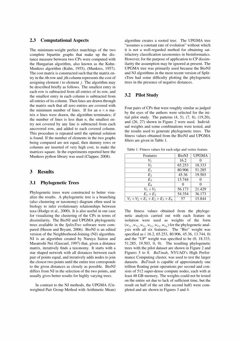
Table 1: Fitness values for each edge and vertex feature.
Features BioNJ UPGMAV1 16.2 0V2 65.253 18.333E1 80.906 51.285E2 45.36 19.503E3 13.744 0E4 0 0
V1 +V2 56.173 21.429E1 +E2 54.354 36.173
V1 +V2 +E1 +E2 +E3 +E4 57 15.844
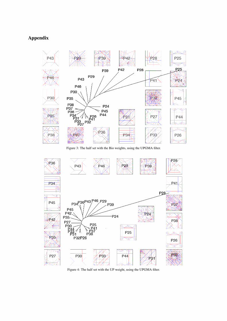
The fitness values obtained from the phyloge-netic analysis carried out with each feature inisolation were used as weights of the form(wv1 ,wv2 ,we1 ,we2 ,we3 ,we4 ) for the phylogenetic anal-ysis with all six features. The “Bio” weight wasspecified as ( 16.2, 65.253, 80.906, 45.36, 13.744, 0)and the “UP” weight was specified to be (0, 18.333,51.285, 19.503, 0, 0). The resulting phylogenetictrees with the pilot dataset are shown in Figure 2 andFigures 5 to 8. BuTinah, NYUAD’s High Perfor-mance Computing cluster, was used to test the largerdatasets. BuTinah is capable of approximately onetrillion floating point operations per second and con-sists of 512 super-dense compute nodes, each with atleast 48 GB memory. The weights could not be testedon the entire set due to lack of sufficient time, but theresult on half of the set (the second half) were com-pleted and are shown in Figures 3 and 4.
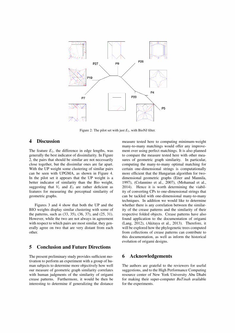
Figure 2: The pilot set with just E1, with BioNJ filter.
4 Discussion
The feature E1, the difference in edge lengths, wasgenerally the best indicator of dissimilarity. In Figure2, the pairs that should be similar are not necessarilyclose together, but the dissimilar ones are far apart.With the UP weight some clustering of similar pairscan be seen with UPGMA, as shown in Figure 4.In the pilot set it appears that the UP weight is abetter indicator of similarity than the Bio weight,suggesting that V1 and E3 are rather deficient asfeatures for measuring the perceptual similarity ofgeometric graphs.
Figures 3 and 4 show that both the UP and theBIO weights display similar clustering with some ofthe patterns, such as (33, 35), (36, 37), and (25, 31).However, while the two are not always in agreementwith respect to which pairs are most similar, they gen-erally agree on two that are very distant from eachother.
5 Conclusion and Future Directions
The present preliminary study provides sufficient mo-tivation to perform an experiment with a group of hu-man subjects to determine more objectively how wellour measure of geometric graph similarity correlateswith human judgments of the similarity of origamicrease patterns. Furthermore, it would be then beinteresting to determine if generalizing the distance
measure tested here to computing minimum-weightmany-to-many matchings would offer any improve-ment over using perfect matchings. It is also plannedto compare the measure tested here with other mea-sures of geometric graph similarity. In particular,computing the many-to-many optimal matching forcertain one-dimensional strings is computationallymore efficient that the Hungarian algorithm for two-dimensional geometric graphs (Eiter and Mannila,1997), (Colannino et al., 2007), (Mohamad et al.,2014). Hence it is worth determining the viabil-ity of converting CPs to one-dimensional strings thatcan be tackled with one-dimensional many-to-manytechniques. In addition we would like to determinewhether there is any correlation between the similar-ity of the crease patterns and the similarity of theirrespective folded objects. Crease patterns have alsofound application to the documentation of origami(Lang, 2012), (Akitaya et al., 2013). Therefore, itwill be explored how the phylogenetic trees computedfrom collections of crease patterns can contribute tothis documentation, as well as inform the historicalevolution of origami designs.
6 Acknowledgements
The authors are grateful to the reviewers for usefulsuggestions, and to the High Performance Computingresource center of New York University Abu Dhabifor making their super-computer BuTinah availablefor the experiments.
REFERENCES
Akitaya, H. A., Mitani, J., Kanamori, and Fukui, Y. (2013).Generating folding sequences from crease patterns offlat-foldable origami. In Proceedings of the SpecialInterest Group on Graphics, pages 991–1000. ACM.
Ambauen, R., Fischer, S., and Bunke, H. (2003). Graph editdistance with node splitting and merging, and its ap-plication to diatom idenfication. In Proc. 4th IAPRIntl. Conf. Graph Based Representations in PatternRecognition, pages 95–106.
Arkin, E. M., Bender, M. A., Demaine, E. D., Demaine,M. L., Mitchell, J. S. B., Sethia, S., and Skiena, S. S.(2004). When can you fold a map? ComputationalGeometry: Theory and Applications, 29(1):166–195.
Balkom, D. J., Demaine, E. D., and Demaine, M. L. (2004).Folding paper shopping bags. In Proceedings of the14th Annual Fall Workshop on Computational Geom-etry, pages 14–15. MIT, Cambridge.
Bern, M. and Hayes, B. (1996). The complexity of flatorigami. In Proceedings of the 7th Annual ACM-SIAMSymposium on Discrete Algorithms, pages 175–183,Atlanta.
Berretti, S., Del Bimbo, A., and Pala, P. (2004). A graph editdistance based on node merging. In Proceedings of theACM International Conference on Image and VideoRetrieval (CIVR), pages 464–472, Dublin, Ireland.
Cheong, O., Gudmundsson, J., Kim, H.-S., Schymura, D.,and Stehn, F. (2009). Measuring the similarity of ge-ometric graphs. In Experimental Algorithms, pages101–112. Springer.
Clapper, B. (2008). Munkres algorithm for the assignmentproblem ver.1.0.6.
Colannino, J., Damian, M., Hurtado, F., Langerman, S.,Meijer, H., Ramaswami, S., Souvaine, D., and Tou-ssaint, G. T. (2007). Efficient many-to-many pointmatching in one dimension. Graphs and Combina-torics, 23:169–178.
Demaine, E. and O’Rourke, J. (2007). Geometric Fold-ing Algorithms: Linkages, Origami, Polyhedra. Cam-bridge University Press, New York.
Demaine, E. D. and Demaine, M. L. (2001). Recent resultsin computational origami. In Origami3: Proc. of the3rd International Meeting of Origami Science, Math,and Education, pages 3–16, Monterey, California.
Eiter, T. and Mannila, H. (1997). Distance measures forpoint sets and their computation. Acta Informatica,34(2):109–133.
Fei, H. and Huan, J. (2008). Structure feature selectionfor graph classification. In Proceedings of the 17thACM conference on Information and knowledge man-agement, pages 991–1000. ACM.
Gao, X., Xiao, B., and Tao, D. (2010). A survey ofgraph edit distance. Pattern Analysis and Applica-tions, 13:113–129.
Gascuel, O. (1997). Bionj: an improved version of the njalgorithm based on a simple model of sequence data.Molecular biology and evolution, 14(7):685–695.
Graham, R. L. (1987). A similarity measure for graphs. LosAlamos Science, pages 114–121.
Gu, C. and Guibas, L. (2011). Distance between foldedobjects. In Proceedings of the European Workshop onComputational Geometry, pages 40–42.
Hodge, T., Jamie, M., and Cope, T. (2000). A myosin familytree. Journal of Cell Science, 113(19):3353–3354.
Huson, D. H. and Bryant, D. (2006). Application of phylo-genetic networks in evolutionary studies. Molecularbiology and evolution, 23(2):254–267.
Kuhn, H. W. (1955). The hungarian method for the assign-ment problem. Naval Research Logistics Quarterly,2(1-2):83–97.
Lang, R. J. (1996). A computational algorithm for origamidesign. In Proceedings of the Twelfth Annual Sym-posium on Computational Geometry, SCG ’96, pages98–105, New York, NY, USA. ACM.
Lang, R. J. (2012). Origami Design Secrets: MathematicalMethods for an Ancient Art. CRC Press.
Levenshtein, V. I. (1966). Binary codes capable of correct-ing deletions, insertions, and reversals. Soviet PhysicsDoklady, 10(8):707–710.
Liapi, K. A. (2002). Transformable architecture inspiredby the origami art: Computer visualization as a toolfor form exploration. In Proceedings of the 2002Annual Conference of the Association for ComputerAided Design In Architecture, pages 381–388.
McArthur, M. and Lang, R. J. (2013). Folding Paper: TheInfinite Possibilities of Origami. Tuttle Publishing,Hong Kong.
Mitani, J. (2011). Oripa origami pattern editor. http://mitani.cs.tsukuba.ac.jp/oripa.
Mohamad, M., Rappaport, D., and Toussaint, G. T. (2014).Minimum many-to-many matchings for computingthe distance between two sequences. Graphs andCombinatorics.
Munkres, J. (1957). Algorithms for the assignment andtransportation problems. Journal of the Society of In-dustrial and Applied Mathematics, 5(1):32–38.
O’Rourke, J. (2011). How to Fold It: The Mathematics ofLinkages, Origami and Polyhedra. Cambridge Uni-versity Press, New York.
Pach, J. (2004). Towards a Theory of Geometric Graphs.No. 342. American Mathematical Society.
Post, O. and Toussaint, G. T. (2011). The edit distance as ameasure of perceived rhythmic similarity. EmpiricalMusicology Review, 6(3):164–179.
Robles-Kelly, A. and Hancock, E. R. (2005). Graph edit dis-tance from spectral seriation. IEEE Trans. on PatternAnalysis and Machine Intelligence, 27(3):365–378.
Tachi, T. (2010). Rigid-foldable structure using bidirection-ally flat-foldable planar quadrilateral mesh. In Ad-vances in Architectural Geometry, pages 87–102.
Wu, W. and You, Z. (2011). A solution for folding rigid tallshopping bags. Proceedings of the Royal Society – A,pages 1–14.
Appendix
Figure 3: The half set with the Bio weights, using the UPGMA filter.
Figure 4: The half set with the UP weight, using the UPGMA filter.
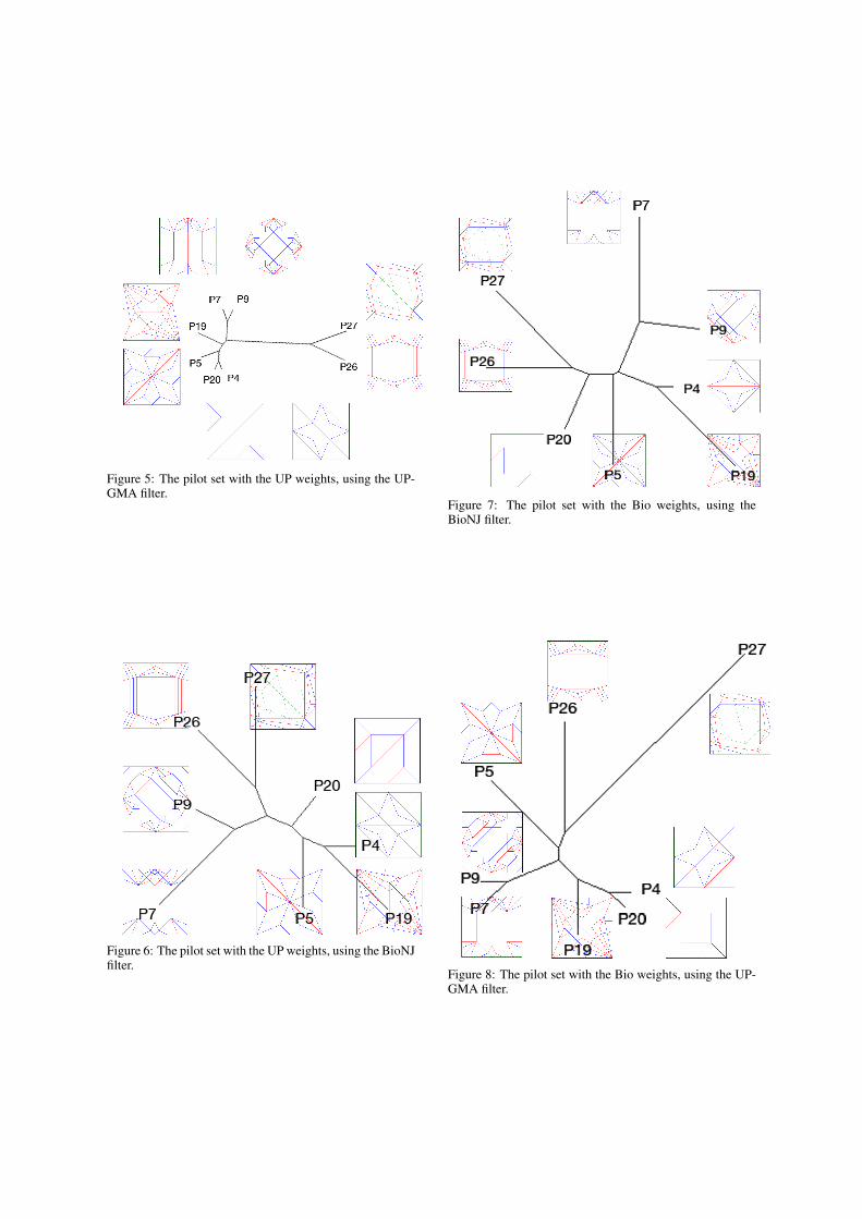
Figure 5: The pilot set with the UP weights, using the UP-GMA filter.
Figure 6: The pilot set with the UP weights, using the BioNJfilter.
Figure 7: The pilot set with the Bio weights, using theBioNJ filter.
Figure 8: The pilot set with the Bio weights, using the UP-GMA filter.