A Dynamic Analysis of Food Demand Patterns in Urban China

Hui Liao and Wen S. Chern

Department of Agricultural, Environmental and Development Economics, The Ohio State University

Selected Paper prepared for presentation at the American Agricultural Economics Association Annual Meeting, Portland, OR, July 29-August 1, 2007

Copyright 2007 by Hui Liao and Wen S. Chern. All rights reserved. Readers may make verbatim copies of this document for non-commercial purposes by any means, provided that this copyright notice appears on all such copies.

1

Abstract

Previous researchers have encountered difficulties in rationalizing the extremely

high expenditure elasticities estimated for grain demanded by urban Chinese households.

The high grain expenditure elasticities, which usually translate into high income

elasticities, are doubtful for making a long-term prediction of grain demand in China.

Unlike most previous studies using only statistic models, this study employs a dynamic

Almost Ideal Demand System (DAIDS) incorporating demographic variables to explore

the impact of habit effects as well as demographic impacts on household level food

demand pattern in urban China. Most dynamic elements and demographic variables are

found significant. The theoretical demand properties cannot be rejected in the DAIDS

model while they are frequently rejected for static models. The dynamic AIDS model

clearly provides improvement in estimating food demand elasticities as compared with

their static counterparts.

Keywords: dynamic almost ideal demand system, habit effect, grain, urban China.

2

I. Introduction

China, with its population surpassing the 1.3 billion mark in 2005, represents the

largest market for agricultural goods and is among the fastest growing economies in the

world during the last two decades. These attributes may be the main reasons that China

has attracted considerable attentions from economists in efforts to assess its abilities to

deal with �Who Will Feed China?� Understanding China�s food demand structure for

predicting its long-term food demand, especially grain demand, is essential in these

investigations. In this paper, we will focus on analyzing the expenditure elasticity of

grain demand by urban Chinese households because of its role in a long-term projection.

Most of previous studies on urban China food demand analysis used static

models, such as extended linear expenditure system (ELES, Lewis and Andrews, 1989),

linear expenditure system and quadratic expenditure system (LES and QES, Chern and

Wang, 1994), linear almost ideal demand system (LA/AIDS, Wu, et al., 1995), quadratic

almost ideal demand system (QAIDS, Liu 2003). These studies often offered conflicting

elasticity estimates (Chern, 1997). In particular, many studies found high expenditure

elasticities (nearly or greater than unity) for grain (e.g., Chen, 1996; Han and Wahl, 1998;

Chern, 1997, 2000; Liu, 2003). The high grain expenditure elasticities usually translate to

high income elasticities where, if used for forecasting, would yield doubtful predictions

for long-term grain demand in China (World Bank, 1997). Accuracy of estimating grain

demand elasticity is important because of its implication to China�s long-term food

security as well as world food security.

Grain is the Chinese traditional main staple food. Most Chinese purchase a certain

amount of grains before allocating their remaining budget among other non-staple foods,

3

such as animal products, fruits and the like. Therefore, we would expect a slow

adjustment or habit effect for grain consumption among China�s urban households.

Because static demand models assume that the consumer can immediately and fully

adjust to changes in prices and income and ignore the dynamic structure caused by habit

formation, they might lead to functional form misspecifications and a relatively low

explanatory power (Shukur, 2002). We suspect that lack of incorporating dynamic

elements leads to the doubtful high grain elasticity.

In this paper, we employ a dynamic generalization of the almost ideal demand

system (AIDS) developed by Ray (1984) to analyze the consumption patterns based on a

two-year urban China household panel data. Ray�s dynamic AIDS (DAIDS) model

incorporates habit effect elements from past consumption and is derived from a

generalized cost function used by Deaton and Muellbauer (1980). It satisfies globally

homogeneous of degree one in current price (Blanciforti et al., 1986), adding-up, and

symmetry.

This study contributes to the existing literature in three ways. First, even though

various dynamic almost ideal demand systems (Anderson and Blundell 1983 and 1984,

Ray 1984, Blanciforti et al. 1986, Shukur 2002, and Eakins and Gallagher 2003) have

been applied to demand analysis after Deaton and Muellbauer published their AIDS

model and have found improvement in elasticity estimation and functional form

specification, to our best knowledge, there is no dynamic model on food demand in

China. Our study will fill the void. Second, there are little, if any existing dynamic

models incorporate demographic variables. We will explore the dynamic effects as well

as the impact of demographic variables on the demand model specification. Third, as

stated previously, the existing literature of food demand in urban China found doubtful

high expenditure elasticities for grain (e.g., Chen, 1996; Han and Wahl, 1998; Chern,

4

1997, 2000). It is important to examine whether or not the ignorance of dynamic behavior

caused the over estimation of grain expenditure asticities. Our results indeed confirm

this suspect.

The remainder of this paper is organized as follows. In section II, we present the

dynamic almost ideal demand system by incorporating habit effects and other dynamic

parameters together with demographic variables. In section III, the two-year panel data

set used in this paper is discussed. In etric results and elasticity

estimates are reported and interprete n V, additional results from unrestricted

models incorporated with demographic variables and restricted models without

demographic variables are presented. Finally, in section VI, we draw conclusions based

on this study and propose possible future extension.

II. Methodology

Since Deaton and Muellbauer (1980) published their famous �Almost Ideal

Demand System�, AIDS had quickly becom one of the most widely used demand

models because of its theoretical consisten unctional flexibility. It satisfies the

axioms of choice and allows aggregation ove ers. Deaton and Muellbauer also

proposed to convert the nonlinear AIDS l into simplified linear AIDS (LA/AIDS)

model by using so called �stone index� to replace the nonlinear price index. Because of

its simplicity and less computation burde odel was very popular for

empirical demand analysis (Green and Alston, 1990). Green and Alston (1990, 1991)

also hinted that there might be some econometric problems associated with the �stone

index�. Eales and Unnevehr (1993) pointed out a simultaneity issue of the stone index. It

could be correlated with the error term because the budget shares appear on both side of

el

section IV, econom

d. In sectio

e

cy and f

r consum

mode

n, LA/AIDS m

5

the equation. Buse (1994) also argued that if the price index P was not exactly (linearly)

proportional to the stone index P*, there was an errors-in-variable problem coming from

the correlation between the stone index and the error term. Hahn (1994) suggested that

LA/AIDS model was �at best only locally consistent with demand theory� and it had no

satisfactory theoretical properties because �they can violate the symmetry restrictions of

consumer demand theory for most combinations of prices and expenditures.� Hahn

advised empirical demand analysts to employ AIDS instead of LA/AIDS or find other

linear models consistent with utility maximization. These arguments suggest that the

LA/AIDS estimates may be biased and inconsistent. In this paper, we will only

demonstrate the differential results from both LA/AIDS and LA/DAIDS models and

compare the difference between linear and nonlinear models.

Even though many valuable results have been obtained from the AIDS model,

Deaton and Muellbauer (1980) pointed out that influences other than current prices and

current total expenditures should be considered in the model. Among others, they

suggested generalizing and improving their AIDS model by incorporating dynamic

elements. Since then, various dynamic AIDS models have been developed and showed

improvement in demand estimation (Anderson and Blundell, 1983 and 1984; Ray, 1984;

Blanciforti et al., 1986; Shukur, 2002;

behind incorporating dynamic elements is that the static models assume consumers react

instantaneously to the new equilibrium when prices or income change. Of course, it is not

realistic in the real world. �Dynamic adjustment to price and income changes is more

plausible� (Klonaris and Hallam, 2003). Most likely, consumers will have some delay in

response to price or income changes. In other words, adjustments towards a new

equilibrium may be spread over several periods (Phlips 1983).

and Eakins and Gallagher, 2003.) The rationality

6

There are two types of lags (Gracia, Gil, and Angulo, 1998): inertia and habit

persistence. Inertia means consumers only slowly adjust their consumption behavior to

changes of prices and income. The dynamic model associated with this kind of lag is an

autoregressive specification where endogenous variable changes depend on both current

and previous exogenous variables; Habit persistence means past consumption will affect

consumers� current consumption. �In other words, past consumption exerts an important

effect on current consumption because some habits have been developed. A partial

adjustment model is behind this hypothesis where changes in consumption depend on

actual values of exogenous variables and on past consumption levels.� (Gracia, Gil, and

Angulo, 1998).

As summarized by Gracia, Gil, and Angulo (1998), there are mainly three

different ways to incorporate dynamic elements in the demand analysis: (1) modifying

the intercept term αi in the demand system equations (Blanciforti and Green,1983;

Blanciforti et al., 1986; ,

2003); (2) estimating the model in the first or four differences (Eales and Unnevehr 1988,

Moschini and Meilke 1989) and (3) using a generated dynamic framework such as

Anderson and Blundell (1983) and Ray (1984) ( Burton and Young 1992, et al.

1993, ong those dynamic models, the model

developed by Ray (1984) is derived directly from a generalized AIDS cost function and

satisfies all economic properties in duality. Ray�s model take care of the second type of

lag, habit persistence, by incorporating past consumption. In addition, as we mentioned

above, grain is the Chinese traditional main staple food. We would assume the existence

of habit persistence in grain consumption. Particularly, the way which Ray incorporates

habit effects implies habit having an income effect on current demand decision. This

Alessie and Kapteyn 1991; Edgerton 1997; Klonaris and Hallam

Kesavan

Gracia, Gil, and Angulo 1998). Am

7

feature is relevant because of our concern on expenditure elasticities. Given the relative

high Engel Coefficients in China, we would expect the model fits China data well. The

other dynamic models such as Anderson and Blundell (1983) are not relevant to this

study because we have panel data only for two years, and this encounter no problems of

serial correlation, stationarity, and co-intergration in time-series analysis.

Following Ray (1984), we define the dynamic AIDS cost function as

∏∑∑∑∑ −+−− +++++=

i

xitjtit

jtijij

iit

iiit

iit

tiipuppxpepuc 101

~

10 lnln)(21ln),(ln ηββθγαδα

Where eit-1 represents the lagged expenditure of food item i, pit stands for the current

price of item i, xt-1 = Σi eit-1 is the lagged aggregate expenditures, u is the unobservable

utility variable, and αi, δi, βi, ηi, θij, γij (=( jiij

~~γγ + )/2) are parameters to be estimated. The

parameters, θij �s, ηi�s, and δi�s are the dynamic elements of particular interest in this

study. As pointed out by Ray (1984), the ηi�s enable the consumer�s marginal budget

share of an item to change over the sample period. The θij �s enable the real expenditure

compensated cross price responses to also vary over the sample period. Furthermore, the

parameters, δi�s capture the consumption persistence, i.e. the habit effects.

By applying Shephard�s Lemma to the current price of each item and substituting

the unobservable utility variable u, we can obtain the following dynamic AIDS budget

share equations:

wit = αi + Σj (γij + θij xt-1 )ln pjt + (βi + ηi xt-1 )ln (xt / Pt*) + εit, (1)

where wit represents the expenditure share allocated to the ith food item, εit denotes the

stochastic error term, Pt* denotes the dynamic AIDS price index, and xt is the total

expenditure. Similar to its static counterpart, Pt* is given by

8

ln Pt*= α0 + Σi δi eit-1 + Σi αi ln pit + 0.5 *Σi Σj (γij + θij xt-1 )ln pit ln pjt (2)

To analyze the demographic effect, we also incorporate nine demographic

variables. These demographic variables are included by replacing the αi in equations (1)

and (2) with:

αi = αi* + αi1 HSIZE + αi2 MALE + αi2 AGE + αi3 AGE512 + αi4 EDUH + αi5

EDUM + αi6 SD + αi7 GD + αi8 HN (3)

where: HSIZE: number of household members,

MALE: gender of the householder, 1: male, 0: female;

AGE: age of householder;

AGE512: indicator of household with children between 5 and 12 years old, 1: yes,

0: otherwise;

EDUH: indicator of householder with at least a bachelor degree, 1: yes, 0:

otherwise;

EDUM: indicator of householder with at least middle school education but with

no bachelor or above degree, 1: yes, 0: otherwise;

SD: household is in Shandong province, 1: yes, 0: otherwise;

GD: household is in Guangdong province, 1: yes, 0: otherwise;

HN: household is in Henan, 1:yes, 0: otherwise.

In the following context, unless noted, αi in the system is αi in equation (3).

The static AIDS model is similar to its dynamic counterpart without all dynamic

ters. The differences lie in that there are no lagged expenditure eit-1 and lagged

terms in the static AIDS models. In other words, static AIDS

model is nested within DAIDS model by restricted δi,,θij and ηi to zeroes. The LA/AIDS

and LA/DAIDS models are the nested models using an approximation for the price index.

Specifically, the only difference is the price index ln Pt* is replaced with the Stone price

parame

aggregated expenditure xt-1

9

index, (=Σi wit lnPit) for LA/AIDS and (=Σi wit-1 lnPit) for LA/DAIDS. In order to

examine the performance of the DAIDS, it is important to compare it with other three

widely used AIDS models. These three alternative models are listed below:

LA/AIDS: wit = αi + Σj γij ln pjt + βi ln (xt / Pt*) + εit , where ln Pt

* =Σi wit lnPit

LA/DAIDS: wit = αi + Σj (γij + θij xt-1 )ln pjt + (βi + ηi xt-1 )ln (xt / Pt*) + εit,

where ln Pt* =Σi wit-1 lnPit

AIDS: wit = αi + Σj γij ln pjt + βi ln (xt / Pt*) + εit,

where ln Pt*= α0 + Σi αi ln pit + 0.5 *Σi Σj γij ln pit ln pjt

In the DAIDS model, the consumer�s perception of current period �fixed cost�

(lnPt*) depends on current prices pit and on his �standard of living� in the last period as

measured by lagged expenditure (Σi δi eit-1). The parameter δi measures the habit effects

on the price �index�, ln Pt*. We can see that in this manner, the habit effects influence the

demand function only through income effect. For most developed countries with low

Engel coefficients, the income effects can be limited and this manner of incorporating

habit effect in the model may be not �entirely satisfactory� (Blanciforti, at el. 1986). Note

that, Blanciforti, at el. (1986) proposed an alternative DAIDS model, where they replaced

the Σi δi eit-1 in Ray�s DAIDS model with δi eit-1 for individual commodity. The problem

with this method is that the economic restrictions, homogeneity and adding-up, only hold

locally. China, the largest developing country in the world, has relatively high Engel

coefficients. In 2004, Engel coefficients for urban China and rural China still stand at

37.7% and 47.2%, respectively (China Statistical Yearbook 2005.) We would expect to

see a significant income effect on food demand from the habit consumption side and

expect this model to fit China data well.

10

11

ij ij i ij

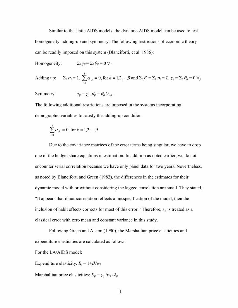
Similar to the static AIDS models, the dynamic AIDS model can be used to test

homogeneity, adding-up and symmetry. The following restrictions of economic theory

can be readily imposed on this system (Blanciforti, et al. 1986):

Homogeneity: Σj γij = Σj θij = 0 ∀i.

Adding up: Σi αi = 1, 9,,2,1for ,08

1⋅⋅⋅==∑

=

ki

ikα and Σi βi = Σi ηi = Σi γij = Σi θij = 0 ∀j

Symmetry: γij = γji, θij = θji ∀i,j.

The following additional restrictions are imposed in the systems incorporating

demographic variables to satisfy the adding-up condition:

9,,2,1for ,08

1⋅⋅⋅==∑

=

ki

ikα

Due to the covariance matrices of the error terms being singular, we have to drop

one of the budget share equations in estimation. In addition as noted earlier, we do not

encounter serial correlation because we have only panel data for two years. Nevertheless,

as noted by Blanciforti and Green (1982), the differences in the estimates for their

dynamic model with or without considering the lagged correlation are small. They stated,

�It appears that if autocorrelation reflects a misspecification of the model, then the

inclusion of habit effects corrects for most of this error.� Therefore, εit is treated as a

classical error with zero mean and constant variance in this study.

Following Green and Alston (1990), the Marshallian price elasticities and

expenditure elasticities are calculated as follows:

For the LA/AIDS model:

Expenditure elasticity: Ei = 1+βi/wi

Marshallian price elasticities: E = γ /w -λ

12

i

For the dynamic LA/AIDS model:

Expenditure elasticity: Ei = 1+(βi + ηi xt-1)/wi

Marshallian price elasticities: Eij = (γij+θij xt-1)/wi -λij

For the AIDS model:

Expenditure elasticity: Ei = 1+βi/wi

Marshallian price elasticities: Eij = [γij -βi (αj + Σk γkj ln Pk)]/wi -λij

For the dynamic AIDS model:

Expenditure elasticity: Ei = 1+(βi + ηi xt-1)/wi

Marshallian price elasticities: Eij = [(γij +θij xt-1) -(βi + ηi xt-1)(αj + Σk γkj ln Pk)]/wi -λij

Where λij is Kroneker�s delta: λij=1 for i=j and 0 otherwise, xt-1, wi, and lnPk will be

calculated at sample means.

Given the relative high Engel coefficients in China, we would expect necessity

food items have positive effects on �fixed cost� (ln Pt*) and δgrain,δoil, δeggs, and δfresh

vegetables to be positive. For meat, fish, and poultry, we would expect these more luxury

food items have negative effects on �fixed cost� and δmeat,δfish, and δpoultry to be negative.

The intuition behind these expectations is that regarding income effect, necessity items

would put more pressure on consumers when they make expenditure decisions because

they have to consume a certain amount of these food items no matter how poor they are.

�Fixed cost� for these items is therefore relatively high. For more luxury items, such

pressure is much less, because consumers may simply choose to consume less or even

none of such items if their incomes don�t allow them to do so. The �fixed cost� is

therefore relatively low. Even though δi does not enter into the elasticity computation

directly, it appears to affect the estimated magnitude of the corresponding β . As to be

shown later, a positive δi is associated with a decreased βi while a negative δi is paired

with an increased βi. These results indicate that without considering the dynamic

specification, the expenditure elasticity for a necessity good would be overestimated

while that for a luxury good would be underestimated in the static models. Because grain

is the traditional Chinese staple food, we would expect a significant positive δi of grain

that drive the grain expenditure elasticity lower.

In the AIDS model, a negative βi implies a necessity good while a positive βi

indicates a luxury good (i.e., with respect to the total expenditure of goods included in the

model). We would expect negative βi�s for grain, oil, eggs, fresh vegetables and positive

βi�s for meat, poultry and fish.

Because adding-up is automatically satisfied, we only impose homogeneity and

symmetry in the systems. Homogeneity and symmetry will be tested with Wald test in the

unrestricted model. Since static model is nested within the dynamic model, we will

perform chi-square test to justify the adoption of dynamic model.

III. Data

A panel dataset from four representative provinces, Shandong, Henan,

Guangdong, and Heilongjiang in China is used. The dataset was obtained from the urban

household surveys conducted by the National Bureau of Statistics (NBS) in China and

covers the years, 2002 and 2003. The four provinces cover Southern China (Guangdong),

Northern China (Heilongjiang), developed and offshore area (Guangdong and Shandong),

and less-developed and inland area (Henan and Heilongjiang). Guangdong is the richest

province among them. For the first time, a revision by keeping the household IDs the

13

same through consecutive year survey adopted by the NBS in 2003 facilitates the creation

14

1 The NBS of China later confirmed our finding on Jiangsu data that the same household ID doesn�t mean same household in both 2003 and 2002 dataset.

of panel data for these two years. To bring as little noise as possible into the system, we

adopt a strict same household matching criteria except for using same household ID. Two

households respectively in 2002 and 2003 datasets are treated as the same household only

when the following three criteria are met: First, household ID, province and city or

county codes, first and second (if applies) household member�s relation to householder,

and householder�s ethnic, gender, and marriage status are the same. Second, first and

second household members� age is one year more in 2003 than 2002. Third, household

members� education level in 2003 is not lower than 2002. We drop the whole Jiangsu

province data because we could not find any household in Jiangsu province that meets the

above criteria.1

The households selected in the surveys are drawn from a large population, based

on proportionate stratification, sampling one out of every 10,000 households. This

database contains detailed household-level data on food consumption. The survey

contains 1,486 variables covering urban household expenditure, income, production,

consumption, as well as household demographic variables. Detailed discussion on the

survey data can be found in Fang, et al. (1998). Totally 2,914 households from this panel

data set are used in this study.

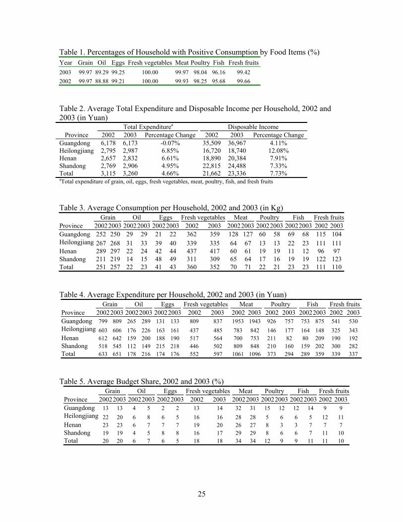
Eight important food items with extremely few households with zero consumption

are selected to avoid censoring problems. They are grain, oil, eggs, meat, poultry, fish,

fresh vegetables, and fresh fruits. The percentages of households with positive

consumption are reported in table 1. The food item with the lowest consumption

percentage is oils, with 88.88% in 2002 and 89.29% in 2003. That means there were

nearly 11% of households who didn�t consume oils in 2002 and 2003. For other food

15

Other major food items not included in this study are: starch, dry bean and bean-made product, shrimp, dry vegetable, sauces, sugar, cigarette, wine, drink, tea, dry fruit, puddings, milk, and food away from home.

items, household consumption percentages are no lower than 95%. These eight foods

accounted for about 50.78% of total food expenditures2 in these four provinces. Grain

consists of rice and flour; meat contains pork, beef and mutton; poultry includes chicken

and duck. The average total expenditure for the eight selected food items and disposable

income per household from the four provinces are reported in table 2. From 2002 to

2003, household disposable incomes increased for all four provinces ranging from 4.11%

to 12.08%. The total expenditures for the eight food items increased for all provinces as

well except Guangdong province where it was dropped merely 0.07%. The poorest

province, Heilongjiang, not only posts the highest disposable income change, also has the

biggest change in total food expenditure. On the contrary, in the richest province,

Guangdong, its disposable income was almost twice as large as that of the second highest

province, but it had is the lowest percentage change in disposable income and posted a

negative growth in total food expenditure. All of the changes in food expenditure are

smaller than the changes in total disposable income. This phenomenon is consistent with

the so-called Engel�s law. The average consumption per household of the eight selected

food items are reported in table 3. The four provinces show similar consumption patterns

in grain, oil, eggs, fresh vegetables, and fresh fruits. Households in Guangdong, the

richest province, consume far more meat, poultry, and fish. Average expenditures per

household are reported in table 4 and average budget shares per household are reported in

table 5. From table 5, we can see that in all four provinces, households allocated a large

percentage of budgets on meat, grain, and fresh vegetables. In Guangdong province,

households allocate smaller budget shares on grain and eggs while spent relatively much

2

more on poultry and fish. Compared with Heilongjiang province, households in Henan

province allocated larger budget shares on grain, eggs, and fresh vegetables but a smaller

share for fresh fruits; In Shandong province, households spent relatively more on eggs

and meat but less on oil and fresh fruits.

IV. Empirical Results and Interpretation

We estimate the four AIDS models, LA/AIDS, LA/DAIDS, AIDS, and DAIDS

incorporating nine demographic variables. Adding-up is automatically satisfied and

homogeneity and symmetry are imposed. In this section, we report and discuss the

estimation results using this model specification. Dynamic models contain lagged

expenditure for each individual food item and lagged total expenditure. The dynamic

elements are used to test whether there are habit effects in urban food consumption in

China.

An iterative Seemingly Unrelated Regressions (ITSUR) procedure in the SAS

package is employed for estimation. The parameter α0 is set to be a-priori the log of the

lowest total expenditure for the eight food items by household following Deaton and

Muellbauer (1980). The budget share function for fresh fruits is dropped in estimation to

avoid the singularity problem.

Appendix table 1 presents the full estimation results for the four AIDS models:

linear AIDS (LA/AIDS) model, linear dynamic AIDS (LA/DAIDS) model, AIDS model,

and dynamic AIDS (DAIDS) model. Most parameters including dynamic elements are

found significant at 5% significance level for all four models. But only AIDS and DAIDS

models yield reasonable signs for most parameters. In the DAIDS model, except eggs, all

16

of the estimated β�s are found significant at 5% level or lower. The estimated β�s are

negative for all necessity food items (grain, oil, eggs, and fresh vegetables) and positive

for all more luxury food items (meat, poultry, and fish) as expected. Except for the oils,

the estimated β�s from AIDS model have the same sign as DAIDS model. While

LA/AIDS and LA/DAIDS models provide mixed signs for β�s. The sign of β determines

the calculated �luxury� or �normal� food items. We can see that the signs of β�s from

DAIDS model are the most plausible. The complete sets of price elasticities estimated

from the fours models are reported in Appendix table 2. The own-price elasticities for the

four AIDS models are also reported in table 6. All of the own-price elasticities are

negative for four models as expected. The four models provide similar own price

elasticities. All four models categorize oil and poultry as elastic goods while label the

others as inelastic ones. The only noticeable own price elasticity difference lies in grain.

The absolute values of own price elasticities for grain are close to unit for LA/AIDS,

LA/DAIDS, and AIDS models. But grain�s own price elasticity from DAIDS model is

only �0.728. These results mean that price changes will only have a large effect on the

demand for oil and poultry but less influence on other goods.

The expenditure elasticities estimated for the four AIDS systems are reported in

table 7. All expenditure elasticities are positive, meaning that all food items selected are

normal goods. For the DAIDS models, grain, oils, eggs, and fresh vegetables can be

categorized as necessity items with expenditure elasticities less than one. As expenditures

on these goods may increase with rising income, but not as fast as income, the proportion

of expenditure on these goods falls as income rises. The expenditure elasticities for meat,

poultry, fish, and fresh fruits are all larger than one. Therefore, as income increases, the

expenditure for these products would raise more relative to other foods such as fresh

17

vegetables. These results also imply that the proportion of expenditure on these goods

may increase as income rises. Note that these elasticities are with respect to the total eight

food item expenditures and not total expenditures (or income). The magnitudes of income

elasticities depend upon the effect of income change on the expenditure of these eight

food items. If this income elasticity is less than unity (which is mostly likely), the income

elasticities for these eight food items would be smaller than the expenditure elasticities

estimated in this study.

In table 7, the LA/AIDS and dynamic LA/AIDS models have high grain

expenditure elasticities of 1.225 and 1.359, respectively, and low expenditure elasticities

for meat of 0.848 and 0.766 and poultry of 0.727 and 0.576. These results are similar to

previous findings of high expenditure elasticities for necessity items and low elasticities

for more luxury items from LA/AIDS models (Chern and Wang 1994; Chen 1996). As

Shukur (2002) pointed out that static LA/AIDS model might be misspecified, we are not

surprised to see these results. The AIDS model delivers much better results with a grain

expenditure elasticity of 0.831 and 1.191 for meat. Fish and poultry have the highest

expenditure elasticities, which seem to be plausible. But the grain�s elasticity still seems

doubtfully high. Most importantly, the theoretical constraints are not satisfied for the

AIDS model. Both homogeneity and symmetry are rejected at 5% level from a Wald test.

Encouragingly, the dynamic AIDS model not only delivers a much more reasonable set

of expenditure elasticities for almost all of the food items we selected but also satisfies all

the theoretical constraints. Grain has the lowest expenditure elasticity at 0.538, which

appeared to be consistent with declining per capita consumption of grain observed in

recent years in urban China. We do not believe that grain is an inferior good but expect

low expenditure elasticity. Meat, poultry, fish, and fresh fruits all have expenditure

18

elasticities larger than one, meaning that the urban households will consume more of

these food items at a higher rate than other foods when their income increases. Both

homogeneity and symmetry cannot be rejected at 5% level from the Wald test for the

DAIDS model. Furthermore, the Chi-square tests for both restricted and unrestricted

models suggest that the hypotheses test for dynamic elements being all equal to zero are

rejected at 5% level, which strongly support the employment of DAIDS to analyze the

urban China household food demand pattern.

In table 8, the estimated habit effect coefficients are presented. Most of the

estimated δ�s are found at 1% or lower significant level except fresh fruits are found at

10% significant level and eggs are not significant. The signs of the δ�s are as expected as

well, with grain, oil, eggs, fresh vegetables, and fresh fruits being positive and meat,

poultry, and fish being negative. Grain and vegetables have the largest estimated δ

coefficients at 2.681 and 2.447. These findings are similar to Ray�s (1984) where food

and clothing have positive δ�s while drinks and fuel have negative δ�s. As we mentioned

earlier, δ�s do not enter into elasticity computation directly but affect the expenditure

elasticity through βi. From table 9, we can see that positive δi lead to a decreased βi while

negative δi lead to an increased βi except for fresh fruits, which is derived from the

adding-up condition. As we noted earlier, these coefficients capture the habit effects of

lagged purchases of the individual items at previous purchases

do affect current consumption and strong habit effects exist in urban Chinese households.

Without considering these dynamic effects, the demand models may be misspecified and

elasticities for necessity items may be overestimated and more luxury food items be

underestimated. Given the trend that average income in urban China has been increasing

and Engel Coefficients decreasing steadily, we might expect the habit effects would

. These results support th

19

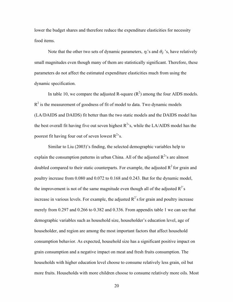
lower the budget shares and therefore reduce the expenditure elasticities for necessity

food items.

Note that the other two sets of dynamic parameters, ηi�s and θij �s, have relatively

small magnitudes even though many of them are statistically significant. Therefore, these

parameters do not affect the estimated expenditure elasticities much from using the

dynamic specification.

In table 10, we compare the adjusted R-square (R2) among the four AIDS models.

R2 is the measurement of goodness of fit of model to data. Two dynamic models

(LA/DAIDS and DAIDS) fit better than the two static models and the DAIDS model has

the best overall fit having five out seven highest R2�s, while the LA/AIDS model has the

poorest fit having four out of seven lowest R2�s.

Similar to Liu (2003)�s finding, the selected demographic variables help to

explain the consumption patterns in urban China. All of the adjusted R2�s are almost

doubled compared to their static counterparts. For example, the adjusted R2 for grain and

poultry increase from 0.080 and 0.072 to 0.168 and 0.243. But for the dynamic model,

the improvement is not of the same magnitude even though all of the adjusted R2�s

increase in various levels. For example, the adjusted R2�s for grain and poultry increase

merely from 0.297 and 0.266 to 0.382 and 0.336. From appendix table 1 we can see that

demographic variables such as household size, householder�s education level, age of

householder, and region are among the most important factors that affect household

consumption behavior. As expected, household size has a significant positive impact on

grain consumption and a negative impact on meat and fresh fruits consumption. The

households with higher education level choose to consume relatively less grain, oil but

20

more fruits. Households with more children choose to consume relatively more oils. Most

of the provincial dummy variables are found significant. Compared to Heilongjiang

province, Henan households allocate more budget share to grain as expected. In all three

provinces, households allocate smaller budget shares for oil consumption, which is

consistent with what we find in table 5. The parameter, α3(hn) is negative, which means

households in Henan allocate higher budget shares on meat than those in Heilongjiang,

which is consistent with table 5. The parameter, α4(gd) is positive as expected. As shown in

table 5, households in Guangdong allocate larger budget share for poultry consumption.

The parameter, α5(gd) is negative and α5(sd) is positive are expected. In table 5, households

in Guangdong allocate smaller budget share to egg while households in Shandong

allocate larger budget shares to egg. The parameter, α6(gd) is positive is inline with that

households in Guangdong allocate much larger budget to fish consumption. Other

noticeable findings are: household size has a positive impact on the grain consumption

and a negative impact on meat consumption as expected; Male householders tend to

consume more oils while older households eat more fish and vegetables but less fruits.

The parameter estimates indicate that budget shares of grain will increase 1.19%

but decrease 0.60% in meat when household size increase by one unit (person). Because

grain is the traditional Chinese staple food and meat is mainly an expensive food item,

the results make sense.

The most significant contribution of the demographic variables is from the

provincial dummy variables. Twenty-two out of twenty-four coefficients are found

statistically significant from zero, meaning the regional food consumption difference is

significant among the four provinces.

21

V. Additional Results from Models without Demographic Variables

In this study, we also estimate the four models without incorporating nine

demographic variables for comparing purpose. Detailed regression results are not

presented in this paper. However, we note that similar to the models with demographic

variables, most of the dynamic coefficients are found significant. The signs of habit effect

coefficients are the same as the ones from the demographic models. The only differences

are habit effect coefficients for fresh fruits being found not significant and the magnitude

of habit effect coefficients are nearly one tenth of the coefficients from models with

demographic variables.

Since we focus on the expenditure elasticities in this study, only the expenditure

elasticities are presented in appendix table 4. Comparing these elasticities with those

presented previously, we find that all expenditure elasticities remain very similar.

Specifically, the expenditure elasticity of grain from DAIDS model without demographic

variables is found at 0.563. Like the DAIDS model with demographic, the DAIDS model

without demographic variables still provides the most reasonable demand elasticity

estimates and has the best fit. But, we want to point out that, as see from above findings,

demographic variables make a significant contribution to the model estimation. Ignorance

of demographic variable is inappropriate.

VI. Conclusions

In this paper, we expand Ray�s DAIDS model by incorporating demographic

variables to analyze urban China household food consumption pattern. We compare the

results from DAIDS with those from LA/AIDS, LA/DAIDS, and AIDS models. The

22

DAIDS model presented in this study provide the best fit overall and the most reasonable

estimation of demand elasticities for the eight food items we select from urban China

dataset.

The empirical results strongly support the presence of habit effects in food

consumption behavior by China urban households. Most of the dynamic coefficients are

found significant at 5% level or lower. All of the habit effect coefficients δ�s except for

eggs are found significant. Six out of eight habit effects are found significant at 1% level.

The signs of the δ�s are as expected with grain, oil, eggs, and fresh vegetables being

positive and meat, fish, poultry being negative. The Wald tests cannot reject the

homogeneity and symmetry in the DAIDS models. Adding-up is automatically satisfied.

Chi-square tests also support the employment of dynamic models. Thus, the dynamic

almost ideal demand system appears to be a viable model to analyze household food

demand in urban China. Similar to previous studies, the static AIDS models yield

doubtful high grain expenditure elasticities. But the DAIDS model delivers a much lower

grain expenditure elasticity of 0.538. Our findings also suggest that a dynamic

specification should work well for food demand analysis in rural China since rural China

has a higher Engel coefficient. One may find stronger consumption persistence by rural

Chinese households, particularly in grain. Unfortunately, a panel data cannot be

constructed from the NBS� rural household survey data.

Even though we have found encouraging results by employing the DAIDS model,

much more can be done in this area. We would conduct future work to improve our

model specification and estimation. First, we will test and compare the DAIDS model

with other dynamic model specifications, especially those proposed by Anderson and

Blundell to see if there exists another model, which can fit the urban China data better.

23

Second, we will extend the model to include other foods with frequent zero consumption

at the household level and therefore we have to deal with the censoring problem. Third,

we would like to have a longer time series of the panel data. Our study is limited with

only two years� data. It is more desirable to have a long time-series for investigating

dynamic behavior.

24

25

Table 1. Percentages of Household with Positive Consumption by Food Items (%) Year Grain Oil Eggs Fresh vegetables Meat Poultry Fish Fresh fruits2003 99.97 89.29 99.25 100.00 99.97 98.04 96.16 99.42 2002 99.97 88.88 99.21 100.00 99.93 98.25 95.68 99.66 Table 2. Average Total Expenditure and Disposable Income per Household, 2002 and 2003 (in Yuan)

Total Expenditurea Disposable Income Province 2002 2003 Percentage Change 2002 2003 Percentage Change

Guangdong 6,178 6,173 -0.07% 35,509 36,967 4.11% Heilongjiang 2,795 2,987 6.85% 16,720 18,740 12.08% Henan 2,657 2,832 6.61% 18,890 20,384 7.91% Shandong 2,769 2,906 4.95% 22,815 24,488 7.33% Total 3,115 3,260 4.66% 21,662 23,336 7.73% aTotal expenditure of grain, oil, eggs, fresh vegetables, meat, poultry, fish, and fresh fruits Table 3. Average Consumption per Household, 2002 and 2003 (in Kg) Grain Oil Eggs Fresh vegetables Meat Poultry Fish Fresh fruitsProvince 2002 2003 20022003 20022003 2002 2003 20022003 20022003 20022003 2002 2003Guangdong 252 250 29 29 21 22 362 359 128 127 60 58 69 68 115 104Heilongjiang 267 268 31 33 39 40 339 335 64 67 13 13 22 23 111 111Henan 289 297 22 24 42 44 437 417 60 61 19 19 11 12 96 97 Shandong 211 219 14 15 48 49 311 309 65 64 17 16 19 19 122 123Total 251 257 22 23 41 43 360 352 70 71 22 21 23 23 111 110 Table 4. Average Expenditure per Household, 2002 and 2003 (in Yuan) Grain Oil Eggs Fresh vegetables Meat Poultry Fish Fresh fruitsProvince 2002 2003 20022003 20022003 2002 2003 2002 2003 2002 2003 20022003 2002 2003Guangdong 799 809 265 289 131 133 809 837 1953 1943 926 757 753 875 541 530 Heilongjiang 603 606 176 226 163 161 437 485 783 842 146 177 164 148 325 343 Henan 612 642 159 200 188 190 517 564 700 753 211 82 80 209 190 192 Shandong 518 545 112 149 215 218 446 502 809 848 210 160 159 202 300 282 Total 633 651 178 216 174 176 552 597 1061 1096 373 294 289 359 339 337

Table 5. Average Budget Share, 2002 and 2003 (%)

Grain Oil Eggs Fresh vegetables Meat Poultry Fish Fresh fruitsProvince 2002 2003 20022003 20022003 2002 2003 20022003 20022003 20022003 2002 2003Guangdong 13 13 4 5 2 2 13 14 32 31 15 12 12 14 9 9 Heilongjiang 22 20 6 8 6 5 16 16 28 28 5 6 6 5 12 11 Henan 23 23 6 7 7 7 19 20 26 27 8 3 3 7 7 7 Shandong 19 19 4 5 8 8 16 17 29 29 8 6 6 7 11 10 Total 20 20 6 7 6 5 18 18 34 34 12 9 9 11 11 10

26

Vegetables 0.057(0.004)*** -0.035(0.003)*** 2.447(0.574)*** Fresh Fruits 0.013a -0.008 a 0.184(0.102)*

Table 6. Comparison of Own-price Elasticities by Model Food item DAIDS AIDS LA/DAIDS LA/AIDSGrain -0.728 -0.958 -0.909 -0.930 Oils -1.082 -1.114 -1.127 -1.121 Meat -0.819 -0.901 -0.839 -0.915 Poultry -0.999 -1.033 -1.025 -1.028 Eggs -0.336 -0.374 -0.345 -0.277 Fish -0.435 -0.479 -0.411 -0.460 Fresh vegetables -0.624 -0.649 -0.710 -0.788 Fresh fruits -0.694 -0.676 -0.703 -0.708

Table 7. Comparison of Estimated Expenditure Elasticities by Model Food item DAIDS AIDS LA/DAIDS LA/AIDSGrain 0.538 0.831 1.359 1.225 Oils 0.778 1.108 1.478 1.297 Meat 1.344 1.191 0.766 0.848 Poultry 1.481 1.169 0.576 0.727 Eggs 0.967 0.848 0.984 0.948 Fish 1.335 1.290 0.825 1.008 Fresh vegetables 0.741 0.802 1.131 1.064 Fresh fruits 1.066 0.911 0.802 0.897

Table 8. Comparison of Habit Effect (δ) from DAIDS

Present Study Ray (1984) Parameters Estimate (S.E.) Parameters Estimate (S.E.) δ1

a 2.681(0.618)*** δFood 0.044(0.006)*** δ2 0.631(0.216)*** δDrinks and Tobacco -0.025(0.018) δ3 -0.524(0.117)*** δFootwear and Clothing 0.009(0.011) δ4 -0.425(0.104)*** δFuel and Light -0.035(0.021)* δ5 0.062(0.152) δ6 -0.319(0.088)*** δ7 2.447(0.574)*** δ8 0.184(0.102)* aThe eight food items are: (1) grain (2) oils, (3) meat, (4) poultry, (5) eggs, (6) fish, (7) fresh vegetables, and (8) fresh fruits *** Significant at 1% level * Significant at 10% level Table 9. Influence of Including Habit Effect (δi) on βi

Estimate of βi Estimate of δiItems DAIDS AIDS DAIDS

Grain -0.111(0.005)*** -0.034(0.004)*** 2.681(0.618)***

Oils -0.013(0.003)*** 0.007(0.002)*** 0.631(0.216)***

Meat 0.119(0.005)*** 0.053(0.004)*** -0.524(0.117)***Poultry 0.036(0.003)*** 0.012(0.002)*** -0.425(0.104)***Eggs -0.001(0.002) -0.01(0.002)*** 0.062(0.152) Fish 0.014(0.002)*** 0.015(0.002)*** -0.319(0.088)***Fresh -

27

***Significant at 1% level * Significant at 10% level aDerived from the adding-up condition. Table 10. Comparison of adjusted R-square (R2) by Model Budget Share Equation DAIDS AIDS LA/DAIDS LA/AIDSGrain (W1) 0.382 0.168 0.241 0.182 Oils (W2) 0.152 0.138 0.173 0.150 Meat (W3) 0.299 0.081 0.130 0.070 Poultry (W4 ) 0.336 0.243 0.287 0.255 Eggs (W5) 0.242 0.240 0.245 0.234 Fish (W6) 0.431 0.373 0.403 0.358 Fresh Vegetables (W7) 0.270 0.170 0.165 0.122

References Alessie, R., and A. Kapteyn. 1991. �Habit Formation, Interdependent References and Demographic Effects in the Almost Ideal Demand System.� The Economic Journal 101(406), 404-19. Anderson, G., and R. Blundell. 1983. �Testing restrictions in a flexible dynamic demand system: an application to consumers� expenditure in Canada.� Review of Economic Studies 50 (3): 397�410. Anderson, G., and R. Blundell. 1984. �Consumer non-durables in the UK: a dynamic demand system.� Economic Journal 94(376a): 35�44. Blanciforti, L.A., R.D. Green, and G.A. King. 1986. �U.S. Consumer Behavior Over the Postwar Period: An Almost Ideal Demand System Analysis.� Giannini foundation Monograph Number 40 (August). Blanciforti, L., and R. Green. 1983. �An Almost Ideal Demand System Incorporation Habits: An Analysis of Expenditures on Food and Aggregate Commodity Groups.� The Review of Economics and Statistics Vol. LXV, No.3. Burton, M.P. and T. Young. 1992. �The structure of changing tastes for meat and fish in Great Britain.” European Review of Agricultural Economics 70(3), 521-32. Buse, A.1994. �Evaluating the Linearized Almost Ideal Demand System.� American Journal of Agricultural Economics Vol. 76, No. 4 (Nov.): 781-793. Chen, J. 1996. �Food Consumption and Projection of Agricultural Demand/Supply Balance for 1996-2005 in China.� Unpublished Master Thesis, Department of Agricultural Economics, The Ohio State University. Chern, W.S. 1997. �Estimated Elasticities of Chinese Grain Demand: Review, Assessment and New Evidence.� A report submitted to the World Bank.

Chern, W.S. 2000. �Assessment of Demand-Side Factors Affecting Global Food Security,� in Food Security in Asia, Edited by W.S. Chern, C.A. Carter, and S.-Y. Shei. Chapter 6: 83-118. Chern, W.S., and G. Wang. 1994. �The Engel Function and Complete Food Demand System for Chinese Urban Households.� China Economic Review 4 (1): 35-57. Deaton, A., and J. Muellbauer. 1980a. �An Almost Ideal Demand System,� American Economic Review (70): 312-326. Eakins, J.M., and L.A. Gallagher. 2003. �Dynamic almost ideal demand systems: an empirical analysis of alcohol expenditure in Ireland.� Applied Economics 35: 1025-1036. Eales, J.S., and L.J. Unnevehr. 1993. �Simultaneity and Structural Change in U.S. Meat Demand.� American Journal of Agricultural Economics Vol. 75, No. 2 (May): 259-268. Edgerton, D.L. 1997. �Weak Separability and the Estimation of Elasticities in Multistage Demand Systems.� American Journal of Agricultural Economics Vol. 79, No. 1 (Feb.): 26-79. Fan, S., and M. Agcaoili-Sombilla. 1997. �Why projections on China's future food supply and demand differ.� The Australian Journal of Agricultural and Resource Economics Volume 41(June): 169. Fang, C., E.J. Wailes, and G.L. Cramer. 1998. �China�s Rural and Urban Household Survey Data: Collection, Availability, and Problems.� Paper presented at the Free Section entitled �Availability and Discrepancy of China�s Agricultural Statistics.� American Agricultrual Economics Association annual meeting, Salt Lake City, Utah, August 1998. Gordon, A., and B. Richard. 1983. �Testing Restrictions in a Flexible Dynamic Demand System: An Application to Consumers� Expenditure in Canada.� Review of Economic Studies L: 397-410. Gracia A., J.M. Gil, and A.M. Angulo. 1998. �Spanish food demand: a dynamic approach.� Applied Economics 30: 1399-1405. Green, R., and J.M. Alston. 1990. �Elasticities in AIDS Models.� American Journal of Agricultural Economics Vol. 72, No. 2 (May): 442-445. Green, R., and J.M. Alston. 1990. �Elasticities in AIDS Models: A Clarification and Extension.� American Journal of Agricultural Economics Vol. 73, No. 3 (Aug): 874-875. Han, T. and T.I. Wahl. 1998. �China�s Rural Household Demand for Fruits and Vegetables.� Journal of Agricultural and Applied Economics 30(July): 141-150.

28

Kesavan, T., Z.A. Hassan, H.H. Jensen, and S.R. Johnson. 1993. �Dynamics and Long-run Structure in U.S. Meat Demand.� Canadian Journal of Agricultural Economics 41, 139-153. Klonaris, S. and D. Hallam. 2003. �Conditional and unconditional food demand elasticities in a dynamic multistage demand system.� Applied Economics 35: 503-514. Lewis, P., and N. Andrews. 1989. �Household Demand in China.� Applied Economics 21: 793-807. Liu, K.E. 2003. �Food Demand in Urban China: an Empirical Analysis Using Micro Household Data.� Ph.D. Dissertation, Department of Agricultural, Environmental, and Development Economics, The Ohio State University. Liu, K.E., and W.S. Chern. 2001. �Effects of Model Specification and Demographic Variables on Food Consumption: Microdata Evidence from Jiangsu, China.� Paper presented at the 11th Annual World Food and Agribusiness Forum, World Food and Agribusiness Symposium of the International Food and Agribusiness Management Association. Sydney, Australia, 27-28 June. Moschini G., and K.D. Meilke. 1990. �Modeling the Pattern of Structural Change in U.S. Meat Demand.� American Journal of Agricultural Economics Vol. 71, No. 2 (May): 253-261. National Bureau of Statistics. 2005. China Statistical Yearbook. China Statistics Press. Phlips, L. 1983. Applied Consumption Analysis. North-Holland Publishing Company, Netherlands. Ray, R. 1984. �A Dynamic Generalisation of the Almost Ideal Demand System.� Economics Letters 14: 235-239. Shukur, G. 2002. �Dynamic specification and misspecification in systems of demand equations: a testing strategy for model selection.� Applied Economics 34: 709-725. World Bank. 1997. At China�s Table: Food Security Options. Washington DC: The World Bank. Wu, Y., E. Li, and S.N. Samuel. 1995. �Food Consumption in Urban China: An Empirical Analysis.� Applied Economics 27: 509-515.

29

30

α5(male) 1.5E-04(0.001) 4.8E-04(0.001) 2.2E-04(0.001) 3.0E-04(0.001) α5(sd) 0.009(0.002)*** 0.009(0.002)*** 0.01(0.002)*** 0.009(0.002)***

Appendix Table 1. Parameter Estimates (with Standard Errors) by Models with Demographic Variables Parameter DAIDS AIDS LA/DAIDS LA/AIDS α1 0.175(0.024)*** 0.22(0.018)*** -0.292(0.03)*** -0.082(0.027)*** α1(age) 1.6E-04(1.4E-04) 3.6E-04(1.6E-04)** 1.7E-04(1.5E-04) -4.2E-04(1.6E-04)*** α1(age12d) -0.001(0.003) -0.003(0.004) -0.001(0.003) 0.001(0.004) α1(edh) -0.042(0.006)*** -0.054(0.007)*** -0.045(0.007)*** -0.049(0.007)*** α1(edm) -0.025(0.006)*** -0.033(0.007)*** -0.029(0.006)*** -0.032(0.007)*** α1(gd) -2.8E-04(0.006) -0.045(0.006)*** -0.017(0.006)** -0.077(0.006)*** α1(hn) 0.016(0.004)*** 0.027(0.004)*** 0.02(0.004)*** 0.026(0.004)*** α1(hsize) 0.012(0.002)*** 0.013(0.002)*** 0.009(0.002)*** 0.002(0.002) α1(male) 0.008(0.003)*** 0.011(0.003)*** 0.007(0.003)** 0.008(0.003)** α1(sd) 0.008(0.004)** -1.0E-04(0.004) 0.004(0.004) 8.6E-05(0.004) α2 0.067(0.01)*** 0.035(0.011)*** -0.12(0.018)*** -0.044(0.016)*** α2(age) 8.2E-06(8.9E-05) -1.0E-05(8.8E-05) -7.0E-05(8.8E-05) -1.2E-04(8.7E-05) α2(age12d) 0.004(0.002)* 0.004(0.002)* 0.005(0.002)** 0.005(0.002)** α2(edh) -0.021(0.004)*** -0.022(0.004)*** -0.018(0.004)*** -0.02(0.004)*** α2(edm) -0.009(0.004)** -0.01(0.004)*** -0.008(0.004)** -0.009(0.004)** α2(gd) -0.021(0.004)*** -0.033(0.004)*** -0.017(0.004)*** -0.032(0.003)*** α2(hn) -0.006(0.003)** -0.006(0.003)** -0.007(0.003)** -0.006(0.003)** α2(hsize) 0.002(0.001) 0.001(0.001) 2.0E-05(0.001) -4.3E-04(0.001) α2(male) 0.008(0.002)*** 0.008(0.002)*** 0.006(0.002)*** 0.007(0.002)*** α2(sd) -0.021(0.003)*** -0.023(0.003)*** -0.019(0.003)*** -0.022(0.003)*** α3 0.203(0.027)*** 0.105(0.022)*** 0.641(0.034)*** 0.467(0.031)*** α3(age) -1.5E-04(1.5E-04) -4.7E-04(1.7E-04)*** -1.9E-04(1.6E-04) 0.001(1.7E-04)*** α3(age12d) -0.005(0.003) -0.002(0.004) -0.004(0.004) -0.007(0.004)* α3(edh) 0.008(0.007) 0.023(0.008)*** 0.012(0.008) 0.017(0.008)** α3(edm) 0.008(0.006) 0.017(0.007)** 0.013(0.007)* 0.015(0.007)** α3(gd) -0.023(0.007)*** 0.013(0.007)* -0.005(0.007) 0.055(0.006)*** α3(hn) -0.009(0.004)** -0.022(0.005)*** -0.016(0.005)*** -0.02(0.005)*** α3(hsize) -0.006(0.002)*** -0.008(0.002)*** -0.004(0.002)* 0.005(0.002)** α3(male) -0.004(0.003) -0.007(0.003)** -0.003(0.003) -0.004(0.004) α3(sd) -0.009(0.004)* -0.002(0.005) -0.006(0.005) -0.002(0.005) α4 0.053(0.012)*** 0.036(0.011)*** 0.259(0.019)*** 0.172(0.016)*** α4(age) -2.7E-04(8.8E-05)*** -3.5E-04(9.2E-05)*** -2.8E-04(9.1E-05)*** -2.0E-05(9.2E-05) α4(age12d) 0.002(0.002) 0.003(0.002) 0.002(0.002) 0.001(0.002) α4(edh) 0.007(0.004)* 0.012(0.004)*** 0.007(0.004)* 0.009(0.004)** α4(edm) 0.001(0.004) 0.004(0.004) 0.002(0.004) 0.004(0.004) α4(gd) 0.065(0.004)*** 0.084(0.004)*** 0.071(0.004)*** 0.096(0.003)*** α4(hn) 0.027(0.003)*** 0.023(0.003)*** 0.025(0.003)*** 0.024(0.003)*** α4(hsize) -0.001(0.001) -0.001(0.001) 4.2E-04(0.001) 0.003(0.001)*** α4(male) -0.001(0.002) -0.002(0.002) 5.3E-05(0.002) -4.0E-04(0.002) α4(sd) 0.017(0.003)*** 0.02(0.003)*** 0.017(0.003)*** 0.02(0.003)*** α5 0.035(0.008)*** 0.063(0.009)*** 0.036(0.016)** 0.063(0.013)*** α5(age) 3.9E-05(6.8E-05) 3.9E-05(6.7E-05) 5.0E-05(6.8E-05) -2.0E-05(6.7E-05) α5(age12d) 0.001(0.002) 0.001(0.002) 0.001(0.002) 0.001(0.002) α5(edh) 0.003(0.003) 0.001(0.003) 0.002(0.003) 0.002(0.003) α5(edm) 0.004(0.003) 0.004(0.003) 0.004(0.003) 0.004(0.003) α5(gd) -0.026(0.003)*** -0.027(0.003)*** -0.027(0.003)*** -0.034(0.003)*** α5(hn) -0.003(0.002) -0.002(0.002) -0.002(0.002) -0.002(0.002) α5(hsize) 0.001(0.001) 0.001(0.001) 0.001(0.001) 3.5E-04(0.001)

31

28

γ33 -0.022(0.015) 0.034(0.011)*** -0.075(0.018)*** 0.024(0.011)** γ34 0.019(0.007)*** 0.003(0.004) -0.002(0.008) 0.003(0.004)

α6 0.066(0.009)*** 0.037(0.009)*** 0.125(0.015)*** 0.062(0.013)*** α6(age) 2.1E-04(6.9E-05)*** 1.3E-04(7.1E-05)* 1.6E-04(7.0E-05)** 2.7E-04(7.2E-05)*** α6(age12d) -0.002(0.002) -0.002(0.002) -0.002(0.002) -0.003(0.002)* α6(edh) 0.002(0.003) 0.003(0.003) 0.003(0.003) 0.004(0.003) α6(edm) 0.002(0.003) 0.004(0.003) 0.004(0.003) 0.004(0.003) α6(gd) 0.033(0.003)*** 0.046(0.003)*** 0.038(0.003)*** 0.057(0.003)*** α6(hn) -0.026(0.002)*** -0.027(0.002)*** -0.027(0.002)*** -0.027(0.002)*** α6(hsize) -0.001(0.001) -0.002(0.001)** -0.001(0.001) 1.6E-05(0.001) α6(male) -0.002(0.001) -0.002(0.001) -0.001(0.001) -0.002(0.002) α6(sd) -0.007(0.002)*** -0.005(0.002)** -0.007(0.002)*** -0.004(0.002)* α7 0.202(0.015)*** 0.28(0.014)*** 0.037(0.023) 0.109(0.021)*** α7(age) 0.001(1.1E-04)*** 0.001(1.1E-04)*** 0.001(1.1E-04)*** 3.2E-04(1.1E-04)*** α7(age12d) -0.001(0.002) -0.003(0.003) -0.002(0.003) 4.0E-04(0.003) α7(edh) 0.017(0.005)*** 0.01(0.005)** 0.015(0.005)*** 0.013(0.005)** α7(edm) 0.007(0.005) 0.003(0.005) 0.005(0.005) 0.003(0.005) α7(gd) 0.009(0.005)** -0.007(0.004) -0.002(0.005) -0.03(0.004)*** α7(hn) 0.034(0.003)*** 0.041(0.003)*** 0.039(0.003)*** 0.04(0.003)*** α7(hsize) -0.002(0.001) -3.4E-04(0.001) -0.003(0.001)* -0.007(0.001)*** α7(male) -0.001(0.002) 4.8E-04(0.002) -0.001(0.002) -0.001(0.002) α7(sd) 0.018(0.003)*** 0.016(0.003)*** 0.018(0.003)*** 0.015(0.003)*** α8 0.2(0.011)*** 0.224(0.013)*** - - α8(age) -0.001(1.1E-04)*** -0.001(1.1E-04)*** - - α8(age12d) 0.002(0.002) 0.002(0.002) - - α8(edh) 0.025(0.005)*** 0.026(0.005)*** - - α8(edm) 0.01(0.005)** 0.011(0.005)** - - α8(gd) -0.038(0.005)*** -0.03(0.004)*** - - α8(hn) -0.034(0.003)*** -0.034(0.003)*** - - α8(hsize) -0.005(0.001)*** -0.003(0.001)** - - α8(male) -0.008(0.002)*** -0.009(0.002)*** - - α8(sd) -0.016(0.003)*** -0.014(0.003)*** - - β1 -0.111(0.005)*** -0.034(0.004)*** 0.066(0.005)*** 0.045(0.004)*** β2 -0.013(0.003)*** 0.007(0.002)*** 0.03(0.003)*** 0.018(0.002)*** β3 0.119(0.005)*** 0.053(0.004)*** -0.052(0.005)*** -0.042(0.004)*** β4 0.036(0.003)*** 0.012(0.002)*** -0.026(0.003)*** -0.02(0.002)*** β5 -0.001(0.002) -0.01(0.002)*** -0.001(0.002) -0.003(0.002)* β6 0.014(0.002)*** 0.015(0.002)*** -0.008(0.002)*** 4.2E-04(0.002) β7 -0.057(0.004)*** -0.035(0.003)*** 0.011(0.004)*** 0.011(0.003)*** γ11 -0.016(0.01) -0.002(0.007) -0.016(0.012) 0.014(0.007)** γ12 -0.015(0.006)*** -0.019(0.003)*** -0.008(0.006) -0.016(0.003)*** γ13 0.023(0.008)*** 0.019(0.006)*** 0.046(0.011)*** 0.011(0.006)* γ14 0.012(0.005)** 0.016(0.003)*** 0.024(0.006)*** 0.012(0.003)*** γ15 -0.007(0.005) -0.006(0.003)** -0.01(0.005)* -0.007(0.003)** γ16 0.003(0.005) 0.011(0.003)*** 0.008(0.005) 0.008(0.003)*** γ17 -0.025(0.006)*** -0.032(0.004)*** -0.051(0.007)*** -0.035(0.004)*** γ18 0.024(0.006)*** 0.014(0.004)*** - - γ22 -0.028(0.007)*** -0.007(0.003)** -0.025(0.007)*** -0.007(0.003)** γ23 0.027(0.008)*** 0.016(0.004)*** 0.032(0.008)*** 0.014(0.004)*** γ24 -0.01(0.005)** 0.001(0.002) -0.008(0.005) 2.1E-04(0.002) γ25 0.009(0.005)* 0.008(0.002)*** 0.005(0.005) 0.007(0.002)*** γ26 0.007(0.004)* -0.002(0.002) 0.006(0.004) -0.003(0.002) γ27 0.001(0.005) -0.002(0.003) -0.007(0.005) -2.0E-05(0.003) γ 0.008(0.005)* 0.004(0.003) - -

32

68

θ77 2.4E-06(1.7E-06) - 1.1E-05(2.5E-06)*** - θ78 -3.3E-07(1.2E-06) - - -

γ35 -0.014(0.007)** -0.015(0.005)*** -0.013(0.008) -0.015(0.005)*** γ36 0.017(0.007)*** -0.018(0.004)*** 0.015(0.007)** -0.016(0.004)*** γ37 -0.011(0.007) -0.009(0.005)* 0.028(0.009)*** 0.007(0.005) γ38 -0.039(0.007)*** -0.031(0.005)*** - - γ44 0.006(0.006) -0.002(0.003) -0.003(0.007) -0.002(0.003) γ45 -0.008(0.004)* 0.006(0.002)*** -0.005(0.004) 0.006(0.002)*** γ46 -0.027(0.004)*** -0.016(0.002)*** -0.029(0.004)*** -0.015(0.002)*** γ47 0.001(0.004) -0.007(0.003)** 0.02(0.005)*** -0.004(0.003) γ48 0.005(0.004) -0.001(0.003) - - γ55 0.064(0.007)*** 0.039(0.004)*** 0.064(0.008)*** 0.047(0.004)*** γ56 0.007(0.004) -0.002(0.002) 0.008(0.005)* -0.005(0.002)* γ57 -0.02(0.004)*** -0.01(0.003)*** -0.024(0.005)*** -0.012(0.003)*** γ58 -0.03(0.004)*** -0.021(0.003)*** - - γ66 -0.02(0.006)*** 0.027(0.003)*** -0.021(0.006)*** 0.028(0.003)*** γ67 0.006(0.004) -3.1E-06(0.002) 0.012(0.005)*** 0.002(0.002) γ68 0.007(0.004) -4.4E-04(0.003) - - γ77 0.044(0.006)*** 0.052(0.004)*** 0.016(0.008)* 0.038(0.004)*** γ78 0.003(0.005) 0.007(0.003)** - - γ88 0.022(0.007)*** 0.029(0.004)*** - - θ11 8.2E-06(2.6E-06)*** - 1.1E-05(3.2E-06)*** - θ12 -9.2E-07(1.6E-06) - -2.7E-06(1.7E-06) - θ13 -5.6E-06(2.1E-06)*** - -1.0E-05(2.8E-06)*** - θ14 -3.1E-07(1.5E-06) - -4.3E-06(1.7E-06)** - θ15 5.8E-08(1.3E-06) - 6.3E-07(1.4E-06) - θ16 1.5E-06(1.3E-06) - -9.8E-07(1.4E-06) - θ17 2.2E-07(1.7E-06) - 8.1E-06(2.0E-06)*** - θ18 -3.1E-06(1.6E-06)** - - - θ22 7.0E-06(2.1E-06)*** - 5.5E-06(2.1E-06)*** - θ23 -5.6E-06(2.2E-06)*** - -6.4E-06(2.4E-06)*** - θ24 3.0E-06(1.4E-06)** - 2.9E-06(1.4E-06)** - θ25 -1.6E-07(1.4E-06) - 1.4E-07(1.4E-06) - θ26 -2.8E-06(1.3E-06)** - -2.2E-06(1.3E-06)* - θ27 3.7E-07(1.3E-06) - 2.3E-06(1.6E-06) - θ28 -9.2E-07(1.3E-06) - - - θ33 2.3E-05(3.7E-06)*** - 3.9E-05(4.9E-06)*** - θ34 -3.8E-06(2.1E-06)* - 2.3E-06(2.4E-06) - θ35 -4.2E-07(1.8E-06) - -1.5E-07(2.2E-06) - θ36 -1.0E-05(1.8E-06)*** - -9.5E-06(2.0E-06)*** - θ37 -5.5E-07(1.9E-06) - -1.0E-05(2.5E-06)*** - θ38 4.0E-06(1.6E-06)** - - - θ44 -2.4E-06(1.8E-06) - 4.4E-07(2.0E-06) - θ45 4.7E-06(1.2E-06)*** - 4.2E-06(1.3E-06)*** - θ46 4.1E-06(1.2E-06)*** - 4.8E-06(1.3E-06)*** - θ47 -3.6E-06(1.2E-06)*** - -9.3E-06(1.6E-06)*** - θ48 -1.7E-06(1.2E-06) - - - θ55 -6.9E-06(1.8E-06)*** - -7.2E-06(2.0E-06)*** - θ56 -3.2E-06(1.2E-06)*** - -3.6E-06(1.3E-06)*** - θ57 3.3E-06(1.2E-06)*** - 4.1E-06(1.4E-06)*** - θ58 2.7E-06(1.0E-06)*** - - - θ66 1.6E-05(1.6E-06)*** - 1.7E-05(1.7E-06)*** - θ67 -1.9E-06(1.1E-06) - -4.4E-06(1.4E-06)*** - θ -2.8E-06(1.0E-06)*** - - -

33

Meat 0.041 0.051 -0.915 0.011 -0.055 -0.057 0.026 -0.102 LA/AIDS Poultry 0.164 0.003 0.040 -1.028 0.079 -0.205 -0.055 0.001

θ88 2.1E-06(1.6E-06) - - - δ1 2.681(0.618)*** - - - δ2 0.631(0.216)*** - - - δ3 -0.524(0.117)*** - - - δ4 -0.425(0.104)*** - - - δ5 0.062(0.152) - - - δ6 -0.319(0.088)*** - - - δ7 2.447(0.574)*** - - - δ8 0.184(0.102)* - - - η1 5.7E-06(9.9E-07)*** - 2.0E-06(6.7E-07)*** - η2 -9.8E-08(6.7E-07) - -3.4E-07(4.3E-07) - η3 -7.4E-06(1.0E-06)*** - -4.3E-06(8.1E-07)*** - η4 -1.4E-07(6.8E-07) - -1.6E-06(4.6E-07)*** - η5 -4.0E-07(5.2E-07) - 1.2E-07(3.8E-07) - η6 1.1E-06(5.6E-07)** - -4.4E-07(3.7E-07) - η7 3.7E-06(7.5E-07)*** - 4.0E-06(5.8E-07)*** - *** Significant at 1% level * Significant at 10% level Appendix Table 2. Marshallian Elasticity Matrix for DAIDS, AIDS, LA/DAIDS, LA/AIDS Models With Demographic Variables

Price of Demand Models

Food Items Grain Oil Meat Poultry Eggs Fish Fresh

Vegetables Fresh Fruits

Grain -0.728 -0.039 0.021 0.041 -0.001 0.037 0.026 0.105 Oil -0.179 -1.082 0.152 -0.011 0.148 -0.020 0.112 0.102 Meat -0.147 -0.001 -0.819 0.039 -0.081 -0.058 -0.154 -0.122 DAIDS Poultry -0.077 -0.052 0.110 -0.999 0.060 -0.197 -0.286 -0.039 Eggs -0.088 0.128 -0.245 0.106 -0.336 -0.054 -0.148 -0.331 Fish -0.020 -0.058 -0.305 -0.265 -0.090 -0.435 -0.103 -0.061 Fresh

Vegetables -0.012 0.041 -0.074 -0.064 -0.039 0.001 -0.624 0.031 Fresh fruits 0.123 0.050 -0.288 0.000 -0.237 -0.020 0.001 -0.694 Grain -0.958 -0.089 0.113 0.083 -0.014 0.053 -0.110 0.090 Oil -0.350 -1.114 0.254 0.009 0.127 -0.027 -0.057 0.050 Meat 0.010 0.051 -0.901 0.005 -0.071 -0.065 -0.087 -0.132 AIDS Poultry 0.160 0.004 0.027 -1.033 0.072 -0.218 -0.141 -0.039 Eggs -0.048 0.136 -0.211 0.105 -0.374 -0.034 -0.108 -0.314 Fish 0.113 -0.042 -0.374 -0.313 -0.070 -0.479 -0.083 -0.043 Fresh

Vegetables -0.119 -0.001 -0.028 -0.031 -0.036 0.001 -0.649 0.061 Fresh fruits 0.181 0.045 -0.320 -0.012 -0.223 -0.004 0.097 -0.676 Grain -0.909 -0.080 0.017 0.052 -0.041 0.026 -0.130 0.066 Oil -0.264 -1.127 0.196 0.022 0.093 -0.021 -0.001 0.102 Meat 0.012 0.043 -0.839 0.020 -0.048 -0.053 -0.029 -0.106 LA/DAIDS Poultry 0.142 0.018 0.076 -1.025 0.117 -0.189 -0.124 -0.015 Eggs -0.129 0.088 -0.207 0.133 -0.345 -0.054 -0.175 -0.311 Fish 0.098 -0.024 -0.283 -0.264 -0.067 -0.411 -0.028 -0.021 Fresh

Vegetables -0.148 0.000 -0.045 -0.051 -0.063 -0.008 -0.710 0.027 Fresh fruits 0.143 0.067 -0.318 -0.012 -0.217 -0.012 0.051 -0.703 Grain -0.930 -0.081 0.057 0.060 -0.033 0.039 -0.175 0.064 Oil -0.268 -1.121 0.234 0.003 0.117 -0.042 0.000 0.076

34

Oil -1.317 -1.331 -1.336 -1.278 Meat -0.966 -0.829 -0.927 -0.812

Eggs -0.102 0.110 -0.236 0.090 -0.277 -0.073 -0.183 -0.329 Fish 0.149 -0.049 -0.299 -0.286 -0.090 -0.460 0.029 0.006 Fresh

Vegetables -0.199 0.000 0.041 -0.023 -0.066 0.008 -0.788 0.027 Fresh fruits 0.138 0.050 -0.307 0.001 -0.229 0.003 0.051 -0.708 Appendix Table 3. Marshallian Demand Elasticity Matrix for LA/AIDS, LA/DIADS, AIDS, DAIDS Models Without Demographic Variables

Price of Demand Models

Food Items Grain Oil Meat Poultry Eggs Fish Fresh

Vegetables Fresh Fruits

Grain -0.969 -0.074 0.154 0.102 -0.039 0.058 -0.221 -0.012 Oil -0.246 -1.317 0.325 0.006 0.219 -0.088 0.016 0.086 Meat 0.112 0.071 -0.966 -0.060 -0.021 -0.157 0.0948 -0.073 LA/AIDS Poultry 0.282 0.005 -0.229 -1.104 0.167 -0.276 0.084 0.071 Eggs -0.121 0.206 -0.090 0.190 -0.442 0.011 -0.151 -0.603 Fish 0.223 -0.102 -0.830 -0.385 0.013 -0.517 0.114 0.484 Fresh

Vegetables -0.251 0.005 0.1483 0.034 -0.055 0.0338 -0.846 -0.070

Fresh fruits -0.026 0.056 -0.220 0.056 -0.419 0.274 -0.135 -0.586 Grain -0.927 -0.075 0.051 0.064 -0.040 0.019 -0.147 0.055 Oil -0.249 -1.331 0.219 0.031 0.188 -0.064 0.049 0.157 Meat 0.037 0.048 -0.829 -0.003 -0.043 -0.106 0.011 -0.113 LA/DAIDS Poultry 0.175 0.026 -0.012 -1.051 0.208 -0.224 -0.073 -0.050 Eggs -0.124 0.178 -0.187 0.237 -0.494 0.033 -0.107 -0.535 Fish 0.074 -0.074 -0.564 -0.313 0.040 -0.421 -0.058 0.315 Fresh

Vegetables -0.167 0.017 0.017 -0.030 -0.039 -0.017 -0.747 -0.034 Fresh fruits 0.120 0.103 -0.340 -0.039 -0.372 0.179 -0.066 -0.584 Grain -1.012 -0.100 0.197 0.108 -0.008 0.053 -0.145 0.087 Oil -0.377 -1.336 0.401 0.040 0.219 -0.051 -0.032 0.091 Meat 0.069 0.079 -0.927 -0.031 -0.064 -0.125 -0.028 -0.160 AIDS Poultry 0.183 0.012 -0.175 -1.052 0.100 -0.234 -0.139 -0.085 Eggs -0.012 0.224 -0.153 0.161 -0.460 0.013 0.005 -0.528 Fish 0.057 -0.090 -0.764 -0.338 -0.035 -0.459 -0.189 0.267 Fresh

Vegetables -0.158 0.004 0.067 -0.014 -0.001 -0.016 -0.692 0.019 Fresh fruits 0.202 0.077 -0.361 -0.021 -0.368 0.193 0.042 -0.523 Grain -0.780 -0.037 0.064 0.048 0.010 0.027 0.015 0.089 Oil -0.140 -1.278 0.219 -0.013 0.261 -0.068 0.204 0.158 Meat -0.108 0.007 -0.812 0.023 -0.082 -0.099 -0.129 -0.130 DAIDS Poultry -0.079 -0.069 0.008 -0.984 0.126 -0.218 -0.304 -0.092 Eggs -0.038 0.231 -0.238 0.194 -0.489 0.016 -0.053 -0.539 Fish -0.082 -0.129 -0.568 -0.295 -0.017 -0.464 -0.180 0.254 Fresh

Vegetables -0.003 0.070 -0.016 -0.056 -0.003 -0.010 -0.626 -0.017 Fresh fruits 0.080 0.075 -0.335 -0.038 -0.389 0.162 -0.117 -0.570 Appendix Table 4. Comparison of Own-price Elasticities by Models without Demographic Variables Food item LA/AIDS LA/DAIDS AIDS DAIDSGrain -0.969 -0.927 -1.012 -0.780

35

Poultry -1.104 -1.051 -1.052 -0.984 Eggs -0.442 -0.494 -0.460 -0.489 Fish -0.517 -0.421 -0.459 -0.464 Fresh vegetables -0.846 -0.747 -0.692 -0.626 Fresh fruits -0.586 -0.584 -0.523 -0.570 Appendix Table 5. Comparison of Estimated Expenditure Elasticities by Models without Demographic Variables Food item LA/AIDS LA/DAIDS AIDS DAIDS Grain 1.214 1.444 0.818 0.563 Oil 1.331 1.611 1.045 0.658 Meat 0.891 0.751 1.187 1.331 Poultry 0.844 0.437 1.390 1.612 Eggs 0.876 1.010 0.749 0.916 Fish 1.113 0.624 1.552 1.481 Fresh vegetables 1.036 1.169 0.791 0.662 Fresh fruits 0.720 0.707 0.759 1.131