© APSA 2003.

A Dynamic Calculus of Voting*

James Fowler† Oleg Smirnov‡ University of California, Davis University of Oregon

August 26, 2003

Abstract

We construct a decision-theoretic model of turnout, in which individuals maximize their subjective expected utility in a context of repeated elections. In the model a nonnegative signaling motivation to vote exists for all citizens, regardless of their ideology or beliefs about the closeness of the election, and is proportional to a citizen's external efficacy, patience, and electoral pessimism. We find tentative support for all three effects in an empirical model of turnout using NES data (1976-1988). This paper suggests that the signaling motivation may play a role in a citizen’s decision to vote. Key words Turnout, voting, elections, signaling motivation, external efficacy. *We would like to thank John Aldrich, Jim Alt, Stephen Ansolabehere, Robert Bates, Henry Brady, Lars-Erik Cederman, Robert Franzese, Gary King, John Londregan, Ken Shepsle, and participants in the workshop on Empirical Implications of Theoretical Models at Harvard University, Summer 2002, for helpful comments. †Department of Political Science, University of California, Davis, One Shields Avenue, Davis, CA 95616. (530) 752-1649. E-mail: jhfowler@ucdavis.edu. ‡Department of Political Science, University of Oregon, Eugene, OR 97403-1284. (541) 684-8739. E-mail: osmirnov@darkwing.uoregon.edu.

1

For the past fifty years, an explanation for why people vote in large electorates has been a

remarkable problem for rational choice theory. Rational choice scholars have primarily focused

on models of turnout that rely on the pivotal motivation to vote in a single election (Downs 1957;

Riker and Ordeshook 1968; Ferejohn and Fiorina 1974; Ledyard 1984; Palfrey and Rosenthal

1983, 1985). This motivation stems from the belief that there is a small chance that a single vote

will decide the outcome of the election. Although the probability of being the pivotal voter is

extremely small even in highly contested elections, one can still resort to the subjective nature of

beliefs and argue that people may overestimate the probability of casting the pivotal vote.

However, sometimes people actually know that their votes cannot be pivotal (Jackson 1983;

Aldrich 1993), and yet they vote in large numbers despite widespread knowledge that there is a

clear election favorite.

We construct a decision-theoretic model of turnout, in which individuals maximize their

subjective expected utility in a context of repeated elections. We assume that the perceived

probability of being pivotal is strictly zero – no one believes that there is a chance of being

decisive. Instead, the turnout decision is driven by what we call the signaling motivation.1

Suppose that parties are policy-motivated (Wittman 1977) and adjust their platforms in response

to the margin of victory in the previous election. Specifically, several authors have suggested

that winners move their platform towards the extremes to satisfy their own preferences while

losers move towards the median voter in order to improve their chances of winning the next

election (Stigler 1972; Kramer 1977; Stone 1980; Conley 2001; Fowler 2002) The size of the

move depends on the size of the victory – landslides yield big changes in the platforms while

close elections yield little if any change (Bernhard, Nokken, and Sala 2002). If so, then voters

may have a signaling motivation to turnout because they can change the margin of victory in the

2

current election. If the voters believe that ‘all votes count,’ they believe that their vote will affect

party platforms offered in the next election as well as policies that the winner is about to

implement. A vote for the expected winner signals a tolerance for even more extreme platforms,

while a vote for the expected loser signals a preference for platforms closer to the center.

Our model indicates that the signaling motivation exists for all possible beliefs about the

closeness of the election. The size of this signaling motivation is proportional to a citizen's

external efficacy, patience, and electoral pessimism. (1) External efficacy describes the ‘belief in

the influence of one’s actions on the decision of the government’ (Rosenstone and Hansen 1993:

143). Voters with high external efficacy believe that parties pay attention to the electorate (and,

presumably, election results) when they are deciding what policies to offer. (2) Patient citizens

who are willing to wait for future gains will place a higher value on the outcome of future

elections. We therefore expect citizens with higher discount factors to be more likely to vote. (3)

Electoral pessimists are those who expect their favorite party to lose the current election. An

extra vote for a party expected to lose will have a small impact on the margin of victory, but an

extra vote for a party expected to win 100% of the vote will not change the margin of victory at

all—it will still win by 100%. We show that the impact of a single vote on the margin of victory

decreases as the expected margin of victory increases. Thus, the worse a voter expects her

favorite party to do in the election, the greater her incentive to balance the outcome by voting.

There is not enough space in this article to test our theory exhaustively, but we do

provide limited support for all three of these effects in an empirical analysis of National Election

Studies (NES) data on US Presidential elections from 1976 to 1988. Many studies have

established a relationship between turnout and external efficacy. We extend this research and

suggest both theoretically and empirically that turnout depends on subjective rates of time

3

preference and subjective beliefs about the probability that one's favorite party will win the

election. The model may provide an explanation for the relationship between the closeness of

the election and turnout. When we include variables for the signaling motivation, closeness is no

longer a significant factor for turnout.

Finally, the model generates additional results regarding differences between voters with

extreme and moderate preferences. In the model, a voter with extreme preferences always

chooses the nearest party since that will tend to move both party platforms in the voter's

preferred direction. Moderates, on the other hand, must also consider electoral probabilities.

Voting for the winner would cause the winning platform to be adjusted further away from the

center. Thus, even if a moderate prefers such a party, she may have an incentive to choose the

party that is more likely to lose in order to keep her favorite party from straying too far away

from her own preference. We call this counter-intuitive phenomenon temporal balancing, and

we note that it may help to explain why moderates are more likely than extremists to vote for

their least-preferred party. We also note that this phenomenon complements the directional

voting (Rabinowitz and MacDonald 1989) and institutional balancing literatures (Fiorina 1988;

Alesina and Rosenthal 1995) and may help explain why midterm elections in the US usually

penalize the party of the President (Campbell 1960) and ‘second-order’ elections penalize the

ruling party in parliamentary systems (Reif and Schmitt 1980).

Before proceeding, we want to emphasize the limitations of our approach. Fully-

informed and interested rational voters in large electorates would probably not be willing to vote

if the signaling motivation were the only incentive because the impact of a single vote on the

margin of victory would be minimal. But we do not argue here that the signaling motivation is

the only incentive to vote. Nor do we argue that all voters are fully-informed, interested, and

4

rational. Nor do we argue that our theory should supplant other theories of turnout. Instead, we

concur with Rosenstone and Hansen (1993) and Verba, Schlozman, and Brady (1995) who argue

that there are many factors that contribute to the decision to vote. Classic pivotal models of

turnout have yielded a number of comparative statics results that have been confirmed

empirically (Aldrich 1993). More importantly, other authors have used these comparative statics

to establish a rational basis for turnout behavior, even if it is not fully rational. For example,

resource mobilization theory (see Verba, Schlozman, and Brady 1995) suggests that people with

better resources (like education and experience working in groups) are more likely to vote

because the costs of gathering information and engaging in action are lower. This is a

comparative static that results from the simple Downsian model. Similarly, our model's main

contribution is to suggest comparative statics that might provide a rational basis for behavioral

results like the relationship between turnout and external efficacy. Our model also yields

comparative statics results that are counter-intuitive and that can be tested empirically. We test

some implications here and find limited support for the theory, but there are far too many

implications to test in a single article that is primarily devoted to theory. We encourage others to

join us in future work to test the empirical validity of the signaling incentive to vote. The rest of

this article is organized as follows. We start with a very basic framework and the intuition for our

signaling model (details of the model and proofs are presented in the appendix). In proposition 1

we derive conditions for turnout and in proposition 2 we show what choices voters make if they

do decide to turnout. In the next section we compare the pivotal and signaling motivations for

different expectations about the outcome of the current election. .In the following section we

derive empirical implications for turnout and vote choice from our theoretical model and test

them using NES data. We also draw on recent work in economics (Harrison, Lau, and Williams

5

2002) to show how our model may explain why socioeconomic status (SES) variables are related

to turnout. Finally, we summarize the results and conclude with suggestions for future research.

A dynamic model of the calculus of voting

We develop a formal model of turnout in which there is no pivotal motivation. For

simplicity we assume that, in the voter’s perception, the probability of casting a decisive vote is

strictly zero. We also focus our attention only on the ‘economic and political goals of an

individual,’ (Downs 1957: 6) specifically setting aside arguments about the duty motivation or a

taste for voting because we are interested in exploring how individual self-interest in the

outcome of the political process might affect one's decision to vote.

We also focus on the importance of political efficacy. As Abramson (1983) notes, ‘next

to party identification, no political attitude has been studied more extensively than feelings of

political efficacy.’ In this paper we suggest how external efficacy can yield electoral

involvement. We hope it will reduce the gap between formal modeling and decades of

qualitative and empirical research on a concept that ‘lies at the heart of many explanations of

citizen activity and involvement’ (Verba, Schlozman, and Brady 1995: 346).

We start with a conventional spatial model of electoral competition (most of the formal

discussion is presented in appendix). Citizens have ideal points that are located on a one-

dimensional issue space and two parties compete for their votes in a winner-take-all election by

proposing platforms located somewhere in the issue space. Each citizen prefers the party whose

platform is located closer to her ideal point. In a static model potential voters care only about the

outcome of the current election; in the dynamic model they also care about the future.

6

How does the outcome of the current election affect future elections? One possibility

suggested by the mandates literature is that parties use the margin of victory from the past

election to adjust the platform they offer in the next election (Smirnov and Fowler 2003). Stigler

(1972) and Kramer (1977) were among the first to suggest that the margin of victory in an

election can be ‘valued in itself as a 'mandate' for the victor’ (Kramer 1977: 317). In this case,

larger margins of victory mean the party or candidate ‘can do considerably more’ (Stigler, p. 99).

Examples of benefits from having a mandate include increased patronage, the election of

legislators from marginal districts whose indebtedness to the party leadership ensures a more

cooperative legislature (Kramer 1977: 317), and general political opportunity (Conley 2001).

Thus, a landslide victory may cause changes in policy that shift the status quo more towards the

winners' preferences. The new status quo would then become the new basis for party platforms

in the next election.

Many events between elections might affect party platforms (e.g. terrorist attacks, stock

market crashes, poll results). However, Conley argues that elections are uniquely important

because they ‘convey information about public preferences to elected representatives so that

these representatives know whether or not to adjust the policy agenda.’ (Conley 2001: 1). In

particular, her formal model shows that politicians have an incentive to react appropriately to the

margin of victory in the previous election, or else ‘they will be punished at the polls in the

future’ (Conley 2001: 6). She also shows empirically that large margins of victory are more

likely to yield large policy changes (see also Stone 1980; Fowler 2002).

We formalize voter perception of this party dynamic in the following response function:

(1) 1J J

t tF F Eµ+ = + (see appendix for derivation)

7

where 1J

tF + is party J’s platform for the election at time t+1 and JtF is the platform for the

election at time t. The variable µ denotes the margin of victory for party J in the election at time

t, and is positive for a victory and negative for a loss. The variable E is an efficacy parameter

indicating the magnitude of a party's response to an electoral victory. The sign on E indicates the

preferred direction of movement for party J (negative if J is the left party and positive if J is the

right party). The size of a platform shift is proportional to the margin of victory µ and the

magnitude of E , which is how much a citizen believes parties pay attention to the views of the

electorate. Citizens with low external efficacy do not think the parties adjust their platforms

much in response to electoral outcomes, corresponding to low values of E. Citizens with high

external efficacy believe that parties do react to the electorate, but only in proportion to the

margin of victory. The importance of external efficacy for political participation has been

documented in a rich literature (Rosenstone and Hansen 1993; Lane 1959; Craig and Maggiotto

1982; Finkel 1987; Iyengar 1980; Cassel and Luskin 1988; Huckfeldt and Sprague 1992;

Timpone 1998).

Given these beliefs, why would a citizen choose to vote? The answer may be in a desire

to make sure that her ‘voice’ is heard by the government (Pateman 1970; Mason 1982;

Thompson 1970; Verba and Nie 1972). If we assume citizens believe their vote is not decisive in

the current election, then there is only one variable that they can influence: by voting instead of

abstaining they can change µ , the margin of victory. This in turn changes the platforms offered

by both parties in the next election. Hence, citizens have an incentive to vote that is independent

of the closeness and outcome of the current election. Each voter in every election has the

capacity to signal to parties whether they should move their platforms left or right.2

8

Obviously, this signaling motivation depends critically on subjective beliefs about how

much a single vote can change the margin of victory ( µ∆ ). This is in turn a function of the

number N of people voting, and the expected proportion p of voters choosing the citizen’s

preferred party in the current election:

(2) 2(1 )1p

Nµ −

∆ =+

(see appendix for derivation).

The role of N is straightforward: the more people vote the less important is your ‘voice.’

The role of p requires a bit more explanation. As defined here, it contrasts with pivotal models

where p can represent the probability of either party winning since it is only used to estimate

how close the election will be. Why is this distinction important? Equation (3) shows that the

effect of a single vote on the margin of victory declines as one expects one's favorite party to win

a larger portion of the vote. In fact, when the margin of victory is expected to be 100%, giving

one more vote to one's preferred candidate would not change the 100% margin of victory at all.

Thus, citizens who expect their favorite party to lose should believe they have a greater impact

on the margin of victory than those who expect their favorite party to win.

The size of this signaling motivation might seem relatively small in large populations

since a citizen can only change the margin of victory by a single vote. However, the perceived

importance of a vote also depends on E, how responsive one thinks the government is.

Moreover, if voters believe parties update their platforms as shown above, then the effect of any

decision made in the current election will persist since platforms in this election become the

basis for platforms in the next election, the election after that, and so on.3 Citizens who choose

to vote in the current election thus capture a discounted stream of benefits for moving platforms

in their preferred direction for all future elections. This means that the signaling motivation will

be sensitive to an individual's discount factor δ .

9

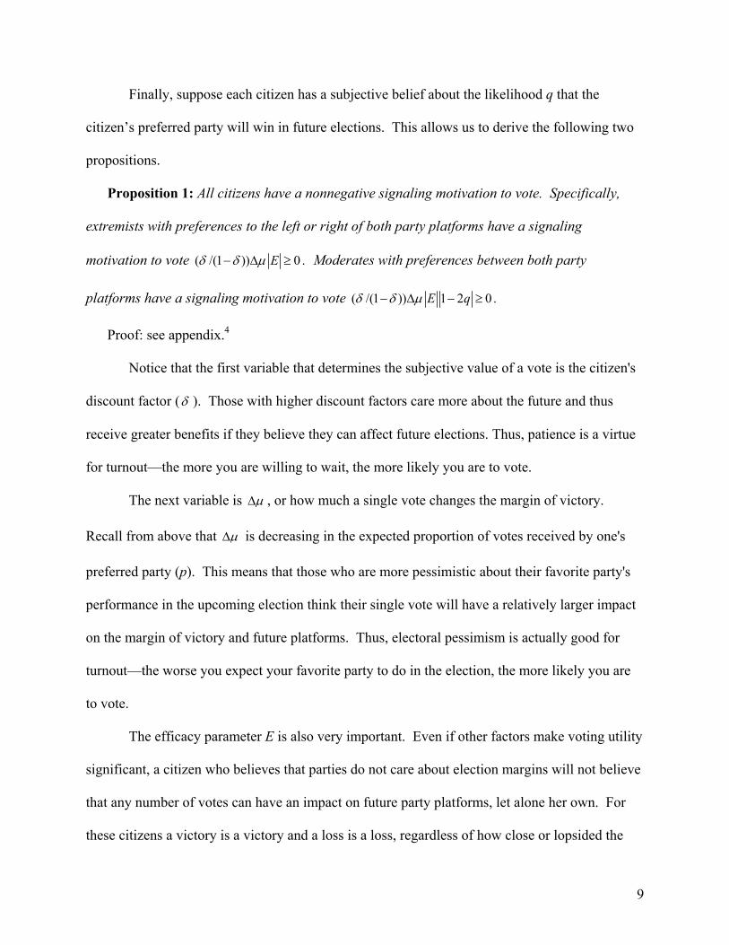
Finally, suppose each citizen has a subjective belief about the likelihood q that the

citizen’s preferred party will win in future elections. This allows us to derive the following two

propositions.

Proposition 1: All citizens have a nonnegative signaling motivation to vote. Specifically,

extremists with preferences to the left or right of both party platforms have a signaling

motivation to vote ( /(1 )) 0Eδ δ µ− ∆ ≥ . Moderates with preferences between both party

platforms have a signaling motivation to vote ( /(1 )) 1 2 0E qδ δ µ− ∆ − ≥ .

Proof: see appendix.4

Notice that the first variable that determines the subjective value of a vote is the citizen's

discount factor (δ ). Those with higher discount factors care more about the future and thus

receive greater benefits if they believe they can affect future elections. Thus, patience is a virtue

for turnout—the more you are willing to wait, the more likely you are to vote.

The next variable is µ∆ , or how much a single vote changes the margin of victory.

Recall from above that µ∆ is decreasing in the expected proportion of votes received by one's

preferred party (p). This means that those who are more pessimistic about their favorite party's

performance in the upcoming election think their single vote will have a relatively larger impact

on the margin of victory and future platforms. Thus, electoral pessimism is actually good for

turnout—the worse you expect your favorite party to do in the election, the more likely you are

to vote.

The efficacy parameter E is also very important. Even if other factors make voting utility

significant, a citizen who believes that parties do not care about election margins will not believe

that any number of votes can have an impact on future party platforms, let alone her own. For

these citizens a victory is a victory and a loss is a loss, regardless of how close or lopsided the

10

election is. On the other hand, if a citizen has a strong sense of external efficacy she is more

likely to believe that every vote helps parties shape the platforms they offer in the future. The

more responsive you think parties are to the ‘voice’ of the people as expressed in elections, the

more likely you are to vote.

The variable q, the likelihood of your favorite party winning in the future, decreases the

signaling motivation for moderates. This is because moderates, whose preferences lie between

the party platforms, want to keep the platforms close to the center. If they expect their favorite

party to win the next election, then voting for it now will cause the party to move the platform

towards its own preferences and away from the center. Thus, the signaling motivation to vote for

one's favorite party actually becomes negative when 0.5q > ! Meanwhile, notice that q is not

present in the equation for extremists, whose signaling motivation is always weakly positive.

This is because one’s vote moves platforms of both parties in the voter’s preferred direction

regardless of expected future probabilities. Therefore, a single vote always matters regardless of

the outcome of the current and all future elections. This distinction between extremists and

moderates generates differences not only in the utility of turnout, but in the choice of party, as

shown in the following proposition:

Proposition 2: If no other incentives exist, extremists vote for the party with the closest

platform if ( /(1 )) E cδ δ µ− ∆ > , otherwise they abstain. Moderates vote for the party that is more

likely to lose in the future elections if ( /(1 )) 1 2E q cδ δ µ− ∆ − > , otherwise they abstain.

Proof: see appendix.

Since an extremist always votes for her first choice, the decision-making problem that she

faces is clear: vote if the benefit from voting is greater than the associated cost. A moderate has

to make a more difficult turnout decision. Given the citizen’s belief about how parties respond

11

to elections (equation 2), she knows that a higher margin of victory would lead her preferred

party to move to its extreme, further from her preference point. The same logic applies for the

other party. Obviously a moderate voter is interested in moderate outcomes. By voting for the

party she expects to lose more often in future elections, she decreases the margin of victory for

the winner and thus discourages the adoption of extreme platforms. Hence, moderates do not

vote for their first choice—they balance future platforms by voting for the party they expect to

lose future elections. We call this phenomenon temporal balancing.

Interestingly, this corresponds to similar results in a pivotal voting model developed by

Feddersen and Pesendorfer (1996). They argue that less informed moderates prefer to abstain.

Similarly, moderates in our model who have no information about future electoral probabilities

might assume the two parties are equally likely to win ( 0.5q = ) which would drive the signaling

motivation to vote to zero. More informed moderates, on the other hand, might have some

intuition about the future. For example, a moderate who prefers the Democratic party in the

United States and believes that demographic factors favor the Democratic party may strategically

vote for Republicans in order to make future platforms by the former less extreme. However,

this belief would have to be strong enough to overcome the cost of voting. Since less certainty

yields beliefs closer to 0.5q = , moderates with less information have a smaller signaling

motivation to vote. This might not exceed the cost, yielding abstention by uninformed

moderates. Thus, our model is also consistent with the finding that moderates tend to vote less

often than extremists (Keith et al 1992).

12

Empirical implications

Our model makes at least three testable predictions about turnout. If the signaling

motivation exists for voters, then turnout should be positively associated with external efficacy

(E) and the discount factor (δ ), and negatively associated with expectations about how well

one's favorite party will do (p).5 The strongly positive impact of external efficacy on turnout has

already been widely documented (Rosenstone and Hansen 1993; Colby 1982; Craig and

Maggiotto 1982; Finkel 1987; Iyengar 1980; Cassel and Luskin 1988; Huckfeldt and Sprague

1992; Timpone 1998), but we are not aware of any empirical tests of the other two variables. To

measure p we index respondents according to whether or not they think the election will be

close, which presidential candidate they think will win, and which candidate they prefer.6 We

code p=0 for respondents who think their favorite candidate will lose in an election that is not

close, p=1/3 if the candidate is expected to lose a close election, p=2/3 if the candidate is

expected to win a close election, and p=1 if the candidate is expected to win an election that is

not close.7

To measure δ we note that the NES has asked two questions related to subjective time

preferences. 1) ‘Do you think it's better to plan your life a good way ahead, or would you say life

is too much a matter of luck to plan ahead very far?’ 2) ‘When you do make plans ahead, do you

usually get to carry out things the way you expected, or do things usually come up to make you

change your plans?’ Respondents who answer yes to the first question have a normative

preference for future planning, indicating that in principle it would be good to think about the

future effects of current actions. Those who say yes to the second question have an experiential

preference for future planning, indicating that past efforts to incorporate the future effects of

current actions have yielded successful results. It seems reasonable to assume that a preference

13

for future planning correlates with subjective time preferences. However, the correlation may be

weak and the binary nature of allowable responses means that we can only coarsely divide

respondents into two groups: those with higher discount factors and those with lower discount

factors. To mitigate this problem somewhat, we create a discount factor index that is the average

of the two responses.

Since we are comparing the signaling model of turnout to other rational models, we

include variables related to the pivotal motivation to vote (see the appendix for coding

specifications). These include the benefit of voting as measured by the perceived difference

between the two candidates, and the probability of being pivotal as measured by the perceived

closeness of the election. We also add a variable for civic duty. This addition is especially

challenging for testing our theory about the signaling motivation because it is based on the

following question: ‘If a person doesn't care how an election comes out then that person

shouldn't vote in it.’ A negative answer to this question has often been interpreted to mean that

respondents believe there is an obligation to vote that transcends individual incentives.

However, we note that respondents might also answer negatively to this question if they consider

the impact on future elections important enough to warrant a vote regardless of their incentives

to vote in the current election. Nonetheless, we include it in our model to be sure that we have

controlled for those respondents who answered negatively because they believe in a civic duty of

voting.

We include several other variables related to turnout as controls (see the appendix).

Verba, Schlozman, and Brady (1995) argue that socioeconomic status variables like education

and income are related to turnout because they affect the costs of acquiring information about

politics—higher status individuals are more likely to vote because their costs are lower. They

14

also note the importance of institutional affiliation. In particular, people acquire civic skills in

organizations (writing letters, public speaking, and so on) that may make it easier for them to

participate in politics. Verba, Schlozman, and Brady point out that psychological variables are

important for turnout as well. The more informed people are about politics and the more they

feel that they can understand political issues (internal efficacy), the more likely it is that they will

be able to make a choice at the polls. Moreover, interest in politics and strength of partisan

identification indicate how politically engaged potential voters are, which tends to correlate with

turnout. Turnout has been shown to depend on these three factors in a wide variety of studies

besides Verba, Schlozman, and Brady (e.g. Timpone 1998).

Each additional control reduces the efficiency of estimation, so we follow King,

Keohane, and Verba (1994) in restricting our attention to variables that are correlated with and

causally prior to our variables of interest. Several socioeconomic status, institutional affiliation,

and psychological factors correlate with our variables of interest and might also be causally prior

to them. For example, a taste for future planning might be affected by feelings of personal

security, which could be a function of socioeconomic status. Similarly, perceptions of

government responsiveness and the likelihood one’s favorite candidate will win might be related

to one’s institutional experience and psychological factors related to politics. We therefore

include them as controls.

Granberg and Holmberg (1991) note that self-reported turnout is significantly higher than

aggregate turnout percentages would imply, so we focus on elections in which turnout was

validated in the NES (1976, 1980, 1984, 1988). We model validated turnout using probit with

heteroskedastic-consistent standard errors, but first we must address the problem of missing data.

Listwise deletion restricts the observations to 1976 since this is the only year in which votes were

15

validated and questions about subjective rates of time preferences were asked. We report these

results because this is the default method of dealing with missing data in political science

analyses. However, listwise deletion inefficiently wastes much of the information available in

the NES, and even worse it may produce biased estimates since several independent variables are

correlated with missingness in our dependent variable.8 We therefore also report results based

on multiple imputation of missing data. Details of this procedure and a discussion are provided

in the appendix.

In addition to predictions about turnout, our model also makes predictions about vote

choice. In proposition 2 we show that when no other incentives exist, extremist voters should

always choose the closest party. However, moderates will only choose the closest party if they

think it will lose future elections. We do not have a good empirical proxy for expectations of

future electoral performance, but if we assume that at least some moderates believe their favorite

party is likely to win future elections then moderates should be more likely than extremists to

abandon their first choice. We create a dichotomous dependent variable that is 0 if a respondent

says she will vote for the candidate she places closest to herself on a seven-point liberal-

conservative scale, and 1 if she says she will vote for the candidate she places farther away. We

then define moderates as those who place themselves in between the Democratic and Republican

candidates on the liberal-conservative scale, and all others as extremists.

There are three major controls we include in our vote choice analysis (see the data

appendix for precise specifications). First, the directional voting literature (Rabinowitz and

MacDonald 1989) suggests that voters may choose the candidate who is spatially further away

because she is on the same side of the center of the issue space. In other words, it might be

easier for a moderate liberal to vote for an extreme liberal who is farther away than for a

16

moderate conservative who is closer. We therefore include a control that indicates when a voter

has chosen a second choice candidate who is on the same side of the liberal-conservative scale.

Second, the institutional balancing literature (Fiorina 1988; Alesina and Rosenthal 1995) points

out that some voters who prefer moderate outcomes may split their ticket between the Congress

and the President by voting for candidates from different parties. This would also cause some

voters to abandon their first choice, so we include a control for split-ticket voting. Third, certain

psychological factors may make it more difficult for some voters to choose a candidate who is

further away even if they know it is in their best interests. We therefore include controls for the

ability to discern a strategic option (internal efficacy, political information, and interest in the

campaign), and the level of attachment to the sincere option (strength of party identification). As

in the turnout model, we use both listwise deletion and multiple imputation for missing data and

for our analysis we use probit with heteroskedastic-consistent standard errors.

Results

Table 1 shows estimates of the effect of pivotal, signaling, and civic duty variables on the

probability of voting. Only one variable related to the pivotal motivation is significant — the

candidate differential has a significant effect on turnout, but the perceived closeness of the

election does not. Meanwhile, all three variables related to the signaling motivation are

significant. In particular, respondents with high levels of external efficacy are 12% more likely

to vote than those with low levels. Those who value future planning are 8% more likely to vote

than those who do not. And those who think their favorite candidate will surely win are 7% less

likely to vote than those who think he will surely lose. The civic duty motivation is also

significant at 8%, but recall from above that respondents who believe in a signaling motivation

17

might answer the civic duty question in the same way as those who believe in a normative

obligation to vote. Thus, part of the civic duty effect in the model could be capturing the

signaling motivation, meaning the signaling estimates may be too small and the civic duty

estimate too large.

Unlike several other statistical models of turnout (e.g. Cox and Munger 1989; Berch

1993; Hanks and Grofman 1998; Grofman et al 1998; Shachar and Nalebuff 1999, Alvarez and

Nagler 2000), closeness in our model is insignificant. The closeness variable typically divides

respondents between those who expect a close election and those who expect a landslide. The

variable p further divides respondents who expect a landslide election into two groups—those

who think their favorite candidate will lose (electoral pessimists) and those who think he will

win (electoral optimists). The pivotal model predicts that pessimists will stay home because they

cannot help their favorite candidate who is sure to lose. The signaling model, on the other hand,

predicts that pessimists will be the most likely to vote because they think they will have the

TABLE 1. Effects on the Probability of Turnout Variable Pooled Model

Using Multiple Imputation

Model for 1976 Using Listwise Deletion

Pivotal Motivation Candidate differential (B) 8 (+/- 6) - Closeness of Election (P) - - Signaling Motivation External efficacy (E) 12 (+/- 5) 11 (+/- 10) Discount factor (δ) 8 (+/- 5) 8 (+/- 4) Probability favorite party wins (p) -7 (+/- 5) -16 (+/- 14) Duty Motivation Civic Duty (D) 8 (+/- 3) 7 (+/- 7) Note: Probabilities are based on model in Table A-1 in the Appendix and they reflect the difference in the probability of turnout when each variable is changed from its lowest to its highest observed value holding all other variables at their mean. Simulated coefficients are used to incorporate estimation uncertainty (for details see King, Tomz, and Wittenberg 2001). 95% confidence intervals are shown in parenthesis and estimates not significantly different from zero are not shown.

18

greatest impact on future platforms. The NES data confirm that electoral pessimists do vote

more often (64%) than optimists (58%) and those who think the election will be close (60%).

This suggests that the finding that closeness encourages turnout may be spurious. NES

respondents are much more likely to be electoral optimists (25%) than pessimists (6%), meaning

four out of five of those expecting a landslide also expect their favorite candidate to win. The

average p for this group is thus quite high (0.80 in our specification). The group expecting a

close election has lower average expectations for their favorite candidate and a lower average

value of p (0.58), and is therefore more likely to vote according to the signaling model. Thus,

the closeness variable may be picking up the effect of p, which is supported by the fact that

including p in our model causes the closeness variable to become insignificant.

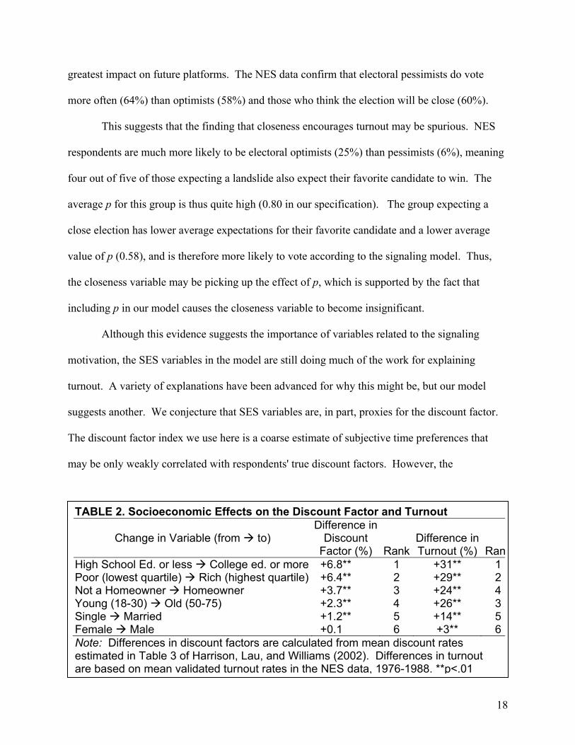
Although this evidence suggests the importance of variables related to the signaling

motivation, the SES variables in the model are still doing much of the work for explaining

turnout. A variety of explanations have been advanced for why this might be, but our model

suggests another. We conjecture that SES variables are, in part, proxies for the discount factor.

The discount factor index we use here is a coarse estimate of subjective time preferences that

may be only weakly correlated with respondents' true discount factors. However, the

TABLE 2. Socioeconomic Effects on the Discount Factor and Turnout

Change in Variable (from to) Difference in

Discount Factor (%)

Rank

Difference in Turnout (%)

RanHigh School Ed. or less College ed. or more +6.8** 1 +31** 1Poor (lowest quartile) Rich (highest quartile) +6.4** 2 +29** 2Not a Homeowner Homeowner +3.7** 3 +24** 4Young (18-30) Old (50-75) +2.3** 4 +26** 3Single Married +1.2** 5 +14** 5Female Male +0.1 6 +3** 6Note: Differences in discount factors are calculated from mean discount rates estimated in Table 3 of Harrison, Lau, and Williams (2002). Differences in turnout are based on mean validated turnout rates in the NES data, 1976-1988. **p<.01

19

experimental economics literature on subjective time preferences has recently made progress in

measuring discount factors and relating them to SES variables. Table 2 shows how education,

income, home ownership, age, marital status, and gender affect discount rates (Harrison, Lau,

and Williams 2002). For example, homeowners are expected to have discount factors that are

3.7% higher than non-homeowners. Notice that the direction of SES effects on discount factors

correlates perfectly with SES effects on turnout. Moreover, notice that the magnitude of the

effects is also strongly correlated ( .88ρ = ). This suggests to us that the causal flow might be

SES variables discount factor turnout.

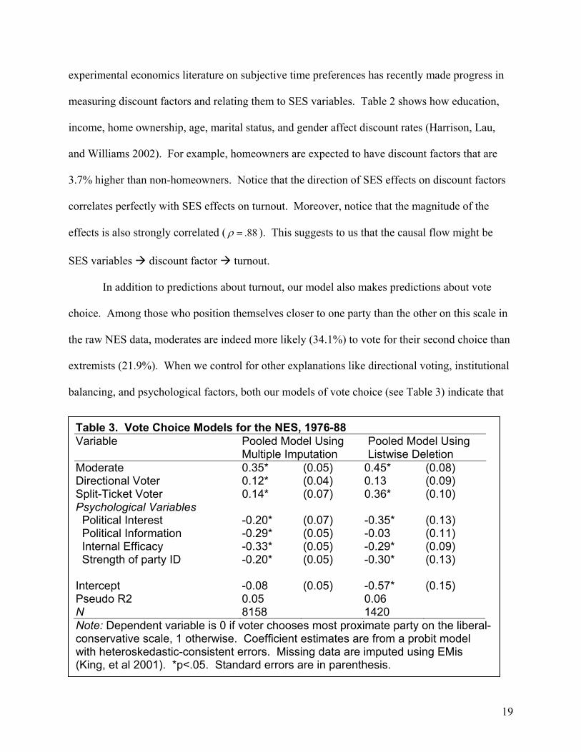
In addition to predictions about turnout, our model also makes predictions about vote

choice. Among those who position themselves closer to one party than the other on this scale in

the raw NES data, moderates are indeed more likely (34.1%) to vote for their second choice than

extremists (21.9%). When we control for other explanations like directional voting, institutional

balancing, and psychological factors, both our models of vote choice (see Table 3) indicate that

Table 3. Vote Choice Models for the NES, 1976-88 Variable Pooled Model Using

Multiple Imputation Pooled Model Using Listwise Deletion

Moderate 0.35* (0.05) 0.45* (0.08) Directional Voter 0.12* (0.04) 0.13 (0.09) Split-Ticket Voter 0.14* (0.07) 0.36* (0.10) Psychological Variables Political Interest -0.20* (0.07) -0.35* (0.13) Political Information -0.29* (0.05) -0.03 (0.11) Internal Efficacy -0.33* (0.05) -0.29* (0.09) Strength of party ID -0.20* (0.05) -0.30* (0.13) Intercept -0.08 (0.05) -0.57* (0.15) Pseudo R2 0.05 0.06 N 8158 1420 Note: Dependent variable is 0 if voter chooses most proximate party on the liberal-conservative scale, 1 otherwise. Coefficient estimates are from a probit model with heteroskedastic-consistent errors. Missing data are imputed using EMis (King, et al 2001). *p<.05. Standard errors are in parenthesis.

20

moderates are 13% more likely to vote for their second choice than extremists.9 This evidence is

consistent with the prediction that moderates engage in temporal balancing, but we admit it is

not definitive. A finer test will require specific questions about perceptions of party strength and

how respondents expect it to change over time.

Conclusion

Our decision-theoretic model focuses on a citizen's subjective but rational estimates of

whether she is better off voting or abstaining. The model emphasizes the value of a vote as a

signal of one's preferences. Three empirical implications of our theoretical model are that

citizens with higher levels of external efficacy, patience, and electoral pessimism should be more

likely to vote. We find limited empirical support for all three implications using validated

turnout from NES data (1976-1988). Turnout is higher among citizens with higher external

efficacy, higher discount factors, and lower expectations about the proportion of votes their

favorite candidate will receive.

We draw several conclusions from our model. First, the analysis suggests why a citizen

may vote when elections are not close and there is a clear favorite. In fact, the signaling

incentive to vote is actually strongest for citizens who expect their favorite candidate to lose in a

landslide. Second, temporal balancing may explain why a voter might rationally support a party

that is farther from her ideal point. This happens when moderates support a party that is more

likely to lose future elections in order to keep future winners from becoming too extreme. Third,

as in Feddersen and Pesendorfer (1996) we provide a rational explanation for why less informed

moderates may be more likely to abstain. Fourth, studies based on the NES that show civic duty

is an important motivation for turnout may, in fact, be capturing the effect of the signaling

21

motivation. The civic duty question asked in the NES does not distinguish between those who

believe in an obligation to vote and those who believe voting is an important signal for future

elections. Fifth, we also suggest that the empirical relationship between the closeness of an

election and turnout is spurious. When we include the expected proportion of votes for one's

favorite candidate in the empirical model, closeness ceases to be significant.

Furthermore, we conjecture that the discount factor may explain why socioeconomic

status variables are related to turnout. In this respect, our model bridges the gap between formal

theory and the large literature on turnout that emerged in the 1950s and 1960s exemplified by

such works as Voting (Berelson, Lazarsfeld, and McPhee 1954) and The American Voter

(Campbell et al 1960). Drawing on recent work in economics, we show that income, education,

age, home ownership, marriage, and gender affect the discount factor in the same direction and

magnitude as they affect turnout. We also speculate that other socioeconomic variables may

have such an effect on the discount factor. For example, Becker and Mulligan (1997: 741) argue

that religious people have higher discount factors because they believe in an afterlife and thus

have longer time horizons. If so, this might explain the strong correlation between church

activity and turnout. Also, blacks may have lower discount rates because of institutional

discrimination, (e.g. less access to credit markets), which in turn might drive their difference in

turnout. These are speculative arguments, but they are meant to illustrate reasons why future

studies of turnout should take discount factors seriously. We urge future election surveys to

include questions about subjective time preferences and experimental studies of discount factors

to keep enough information about their subjects so that their turnout behavior can be validated.

Our analysis may also contribute to literatures on macropolitical economy and spatial

modeling, and institutional balancing. For example, unlike many existing macropolitical

22

economy models our model explains why citizens with extreme preferences may abstain.

Extremists who think parties are not responsive to the electorate or who expect their favorite

party to do well (electoral optimists) get less utility from signaling and are thus less likely to

vote. In a spatial context, we also explain why party platforms might be more stable over time

than otherwise expected. If supporters of the party expected to lose tend to be more motivated

than supporters of the party expected to win, then the result will be negative feedback in an

electoral system that keeps margins of victory closer to zero. Thus parties would have less of an

incentive to make dramatic changes in their platforms, making the system more stable and

slower to change than one might otherwise expect.

Finally, we note that both the negative feedback effect and the tendency of moderates to

engage in temporal balancing may help to explain party surge and decline. Suppose that a party

wins a national election (surge). If this causes voters to increase their estimate of the probability

that the party will win the next election, our model suggests two effects. First, supporters of the

winning party will have less incentive to vote in the next election because they are more

optimistic about their favorite party’s chances. Similarly, supporters of the opposition will have

a greater incentive to vote. As a result, the vote share for the winning party should be lower in

the next election (decline). Second, some moderates may change their mind about who is likely

to win the next election. Since moderates have an incentive to balance by voting for the party

less likely to win future elections, this would increase the vote share for the opposition and

decrease it for the party that recently won (again, decline). Citizens might be relatively more

inclined to use their vote as a signal in lower stakes elections when the pivotal motivation is less

important. Thus, this may be why midterm elections in the US usually penalize the party of the

President (Campbell 1960; Fiorina 1988; Alesina and Rosenthal 1995) and ‘second-order’

23

elections penalize the ruling party in parliamentary systems (Reif and Schmitt 1980). Future

work should examine the impact of the signaling motivation on surge and decline by modeling

change in voter beliefs about electoral probabilities in a context of alternating high stakes and

low stakes elections.

Appendix A: model and propositions

In the model each ‘citizen’ i has an ideal point in one-dimensional issue space 1iQ ∈ℜ and

faces a decision problem to maximize subjective expected utility. The decision problem takes

place in the context of infinitely repeated elections starting with the current election at time 0t = .

In every election two parties (J and ~J) compete with each party proposing a platform 1F ∈ℜ .

Each citizen has three choices: vote for the closest (‘favorite’ or ‘preferred’) party (J), vote for

the party furthest away (~J), or abstain. Citizen i’s single period utility from voting is

| |Vi iU F Q c= − − − , where 0c > is the cost of voting in the current election, and F is platform of

the winning party. Correspondingly the single period utility from abstention is the same except

that a citizen does not incur the cost | |Ai iU F Q= − − . For simplicity we assume that a voter

believes her vote will not change the outcome of the current election (the probability of being

pivotal is 0P = ). Nor does she get extra benefits from voting related to a normative obligation to

vote ( 0D = ).

The total number of ‘voters’ is the sum of votes for each party ~J JN V V= + , which is

different from the total number of ‘citizens’ if there is at least one abstention. Candidate J wins

elections by simple majority rule and the margin of victory for candidate J is

(3) ~J JV VN

µ −= .

24

Notice that if party J loses the election, µ is negative: in this case the ‘margin of victory’ is, in

fact, a margin of a loss. We assume that voters believe that parties use the margin of victory

from the previous election to adjust the platform they offer in the next election. Specifically,

voters think parties act in accordance with an exogenously given response function

(4) 1t tF F Eµ+ = + ,

where 1tF + is a new platform, tF is the previous platform, µ is the past margin of victory, and

E is an ‘efficacy’ parameter denoting how much the voter thinks parties pay attention to citizen

preferences. Furthermore, the sign of E indicates the voter's belief about the preferred direction

of movement for party J ( 0E ≥ if J is the right party and 0E ≤ if J is the left party). This means

that Eµ is positive for both parties when the right wins (they both move right) and negative

when the left wins (they both move left).

Let /Jp V N= be the citizen's expectation of the proportion of votes her favorite party

will receive in the current election. Note that this can also be thought of as the probability that

any other given voter will vote for candidate J. One vote for party J has the following effect on

the margin of victory:

(5) ( ) ~ ~ ~1 2 2(1 )1 ( 1) 1

V J A J J J J JV V V V V pN N N N N

µ µ µ − + − −∆ = − = − = =

+ + +

By the same logic, one vote for party ~J has the exact opposite effect on the margin of victory,

changing it by:

(6) (~ ) ~ ~ ~1 21 ( 1)

V J A J J J J JV V V V VN N N N

µ µ µ− − − −− = − = = −∆

+ +.

A citizen’s decision to vote thus has a direct effect on the platforms both parties offer in the next

election. A vote for party J changes both party platforms by

25

(7) ( )t tF E F E Eµ µ µ µ + + ∆ − + = ∆ .

Moreover, this change in the party platform persists into the future since it becomes the new

basis for future platforms. For example, the effect of a vote today on the platform 2 elections

from now is the same:

(8)

,2 1 1 1

( ),2 1 1 1( ), ,2 2

( )

A tt t t t t t

V J tt t t t t tV J t A t

t t

F F E F E E

F F E F E E

F F E

µ µ µ

µ µ µ µ

µ

+ + + +

+ + + +

+ +

= + = + +

= + = + + ∆ +

− = ∆

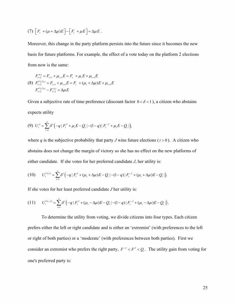
Given a subjective rate of time preference (discount factor 0 1δ< < ), a citizen who abstains

expects utility

(9) ( )~

1| | (1 ) | | ,A t J J

i t t i t t it

U q F E Q q F E Qδ µ µ∞

=

= − + − − − + −∑

where q is the subjective probability that party J wins future elections ( 0t > ). A citizen who

abstains does not change the margin of victory so she has no effect on the new platforms of

either candidate. If she votes for her preferred candidate J, her utility is:

(10) ( )( ) ~

1| ( ) | (1 ) | ( ) | .V J t J J

i t t i t t it

U q F E Q q F E Qδ µ µ µ µ∞

=

= − + + ∆ − − − + + ∆ −∑

If she votes for her least preferred candidate J her utility is:

(11) ( )(~ ) ~

1| ( ) | (1 ) | ( ) |V J t J J

i t t i t t it

U q F E Q q F E Qδ µ µ µ µ∞

=

= − + −∆ − − − + −∆ −∑ .

To determine the utility from voting, we divide citizens into four types. Each citizen

prefers either the left or right candidate and is either an ‘extremist’ (with preferences to the left

or right of both parties) or a ‘moderate’ (with preferences between both parties). First we

consider an extremist who prefers the right party, ~J JiF F Q< < . The utility gain from voting for

one's preferred party is:

26

(12)

( ) ~

1

~

1

( (( ( ) ) ) (1 )(( ( ) ) ))

( ( ) (1 )( )) .1

V J A t J Ji i t i t i

t

t J Jt i t i

t

U U q F E Q c q F E Q c

q F E Q q F E Q E c

δ µ µ µ µ

δδ µ µ µδ

∞

=

∞

=

− = + + ∆ − − + − + + ∆ − − −

+ − + − + − = ∆ −−

∑

∑

The case for a left extremist ( ~J JiQ F F< < ) yields a similar result:

(13)

( ) ~

1

~

1

( ( ( ) ) (1 )( ( ) ))

( ( ) (1 )( )) .1

V J A t J Ji i t i t i

t

t J Jt i t i

t

U U q F E Q c q F E Q c

q F E Q q F E Q E c

δ µ µ µ µ

δδ µ µ µδ

∞

=

∞

=

− = − − + ∆ + − + − − − + ∆ + − −

− − + + − − − + = − ∆ −−

∑

∑

Since 0E ≤ for left extremists and all other variables in the first term are nonnegative, the

signaling motivation to vote for all extremists is:

(14) 01

Eδ µδ∆ ≥

−

If extremists vote for their less preferred party (~J) the sign on µ∆ simply changes and yields

nonpositive utility:

(15) 01

Eδ µδ

− ∆ ≤−

Thus, if no other incentives exist extremists will choose to vote for their preferred candidate

when ( /(1 )) E cδ δ µ− ∆ > . Otherwise they will abstain.

Moderates have different incentives. Consider the case of a right moderate

( ~J JiF Q F< < ). The utility of voting for one's preferred candidate is:

(16)

( ) ~

1

~

1

( ( ( ) ) (1 )( ( ) ))

( ( ) (1 )( )) (1 2 ) .1

V J A t J Ji i t i t i

t

t J Jt i t i

t

U U q F E Q c q F E Q c

q F E Q q F E Q q E c

δ µ µ µ µ

δδ µ µ µδ

∞

=

∞

=

− = − − + ∆ + − + − + + ∆ − − −

− − + + − + − = ∆ − −−

∑

∑

27

For left moderates ( ~J JiF Q F< < ) the result is similar:

(17)

( ) ~

1

~

1

( ( ( ) ) (1 )( ( ) ))

( ( ) (1 )( )) (1 2 ) .1

V J A t J Ji i t i t i

t

t J Jt i t i

t

U U q F E Q c q F E Q c

q F E Q q F E Q q E c

δ µ µ µ µ

δδ µ µ µδ

∞

=

∞

=

− = + − ∆ − − + − − − − ∆ + − −

+ − + − − − + = − ∆ − −−

∑

∑

Since 0E ≤ for left moderates and all other variables in the first term are nonnegative, the

signaling motivation for all moderates is:

(18) (1 2 ) 01

E qδ µδ∆ − ≥

−

If a moderate votes for her less preferred party (~J), the sign on µ∆ changes and so does the

signaling motivation utility:

(19) (2 1) 01

E qδ µδ∆ − ≥

−.

Recall that q is the citizen's belief about the probability that party J will win future elections.

When 0.5q < the utility for voting for party J is positive and the utility for voting for party ~J is

negative. The reverse is true when 0.5q > . Thus moderates only get positive utility from voting

for the party they think is more likely to lose future elections, and they do so only when

( /(1 )) 1 2E q cδ δ µ− ∆ − > . Otherwise, they abstain.

We include one last technical proposition about citizen types. When parties shift their

platforms this causes some citizens with ideal points very close to the platform to change from

being a moderate to an extremist or vice versa as we have defined them. The following

proposition shows that it is the type in the election at time t+1 that determines a citizen’s

strategy.

Proposition 3: The citizen’s strategy in period t is contingent upon her type in period t+1.

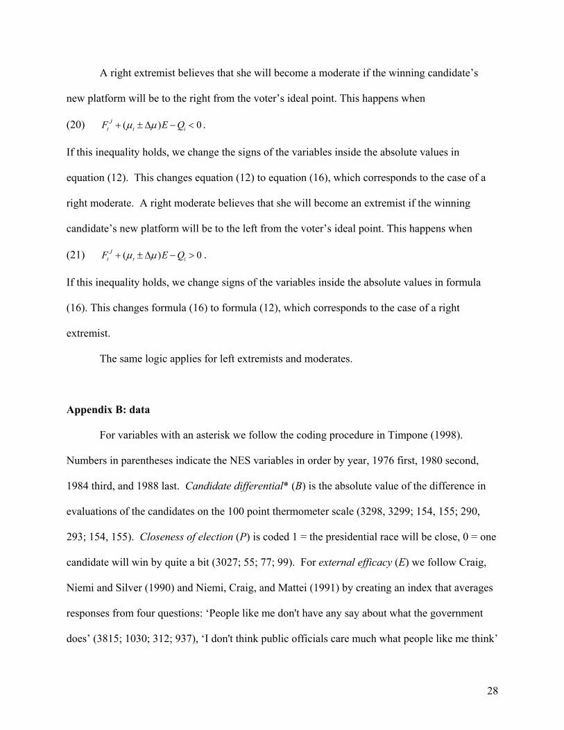
28

A right extremist believes that she will become a moderate if the winning candidate’s

new platform will be to the right from the voter’s ideal point. This happens when

(20) ( ) 0Jt t iF E Qµ µ+ ± ∆ − < .

If this inequality holds, we change the signs of the variables inside the absolute values in

equation (12). This changes equation (12) to equation (16), which corresponds to the case of a

right moderate. A right moderate believes that she will become an extremist if the winning

candidate’s new platform will be to the left from the voter’s ideal point. This happens when

(21) ( ) 0Jt t iF E Qµ µ+ ± ∆ − > .

If this inequality holds, we change signs of the variables inside the absolute values in formula

(16). This changes formula (16) to formula (12), which corresponds to the case of a right

extremist.

The same logic applies for left extremists and moderates.

Appendix B: data

For variables with an asterisk we follow the coding procedure in Timpone (1998).

Numbers in parentheses indicate the NES variables in order by year, 1976 first, 1980 second,

1984 third, and 1988 last. Candidate differential* (B) is the absolute value of the difference in

evaluations of the candidates on the 100 point thermometer scale (3298, 3299; 154, 155; 290,

293; 154, 155). Closeness of election (P) is coded 1 = the presidential race will be close, 0 = one

candidate will win by quite a bit (3027; 55; 77; 99). For external efficacy (E) we follow Craig,

Niemi and Silver (1990) and Niemi, Craig, and Mattei (1991) by creating an index that averages

responses from four questions: ‘People like me don't have any say about what the government

does’ (3815; 1030; 312; 937), ‘I don't think public officials care much what people like me think’

29

(3818; 1033; 313; 938), ‘How much do you feel that having elections makes the government pay

attention to what the people think?’ (3743; 890; 309; 959), and ‘Over the years, how much

attention do you feel the government pays to what the people think when it decides what to do?’

(3741; 888; 310; 960). The first two questions are coded 0 = agree, 0.5 = neither, and 1 =

disagree in 1976-1984. For 1988 they are 0 = agree strongly, 0.25 = agree somewhat, 0.5 =

neither, 0.75 = disagree somewhat, and 1 = disagree strongly. The third and fourth questions are

coded 1 = a good deal, 0.5 = some, and 0 = not much. Coding for the discount factor (δ) (3736,

3737 in 1976 only) and the probability favorite party wins (p) (3026, 3027, 3044, 3045; 54, 55,

137; 76, 77, 425; 98, 99, 763) are described in the text. Civic duty (D) is coded 1 = yes and 0 =

no for ‘If a person doesn't care how an election comes out he shouldn't vote in it.’ (3350; 145;

311; 936)

Education* is the number of years completed (3384; 429; 431; 419). Income* is family

income in constant 1976 dollars, using the Bureau of Labor Statistics measure of the CPI to

transform income in later years (686; 725; 680; 520). Employed is coded 1 = employed and 0

otherwise (3409; 515; 457; 429). Home Ownership* is coded 1 for homeowners, 0 for others

(3509; 719; 706; 552). Age* is in number of years and age-squared* is mean-centered to reduce

collinearity (3369; 408; 429; 417). Marital status* is 1 for married and 0 for all others (3370;

409; 430; 418). Gender* is 1 for female, 0 for male (3512; 720; 707; 413). Race* is 1 for black,

0 for others (3513; 721; 708; 534). South* is 1 for people from southern states, 0 for others.

Church attendance* is an index of religious attendance, 0 = never/no religious preference, 0.25 =

a few times a year, 0.5 = once or twice a month, 0.75 = almost every week, and 1 = every week.

Group membership* is coded 1 if people belong to any organizations representing the group they

feel closest to and 0 otherwise (3868; 1169; 1103; 1114). Political interest in the campaign is

30

coded 1 = very much interested, 0.5 = somewhat interested, 0 = not much interested (3031; 53;

75; 97). Following Verba, Schlozman, and Brady (1995), political information is based on

answers to factual questions: ‘Do you happen to know which party elected the most members to

the House of representatives in the elections this/last month?’(3683; 1028; 1006; 878) and ‘Do

you happen to know which party had the most members in the House of Representatives in

Washington before the elections?’ (3684; 1029; 1007) The second question was not asked in

1988 so we substitute and ‘Do you happen to know which party had the most members in the

Senate before the elections?’ (879 in 1988 only). We code the variable 1 = correct answer to

both questions, 0.5 = correct answer to one question, 0 = no correct answers. Internal efficacy*

is a binary response (0 = true, 1 = false) to the question ‘Sometimes politics and government

seem so complicated that a person like me can't really understand what's going on.’ (3817; 1032;

314; 939) Strength of party identification* is coded 0 = independents and apoliticals, 1/3 =

independents leaning towards a party, 2/3 = weak partisans, and 1 = strong partisans. (3174; 266;

318; 274)

Spatial positioning for variables in the vote choice model are determined by self-

placement and placement of the major party candidates on the liberal-conservative scale (3286,

3287, 3288; 267, 268, 269; 369, 371, 372; 228, 231, 232). Strategic voting is coded 0 if

respondents vote for the candidate they place closest to their own position. Otherwise, it is

coded a 1. (3044, 3045; 137; 425; 397). Moderates are coded 1 if they place themselves between

the two candidates and 0 otherwise. Directional voting is coded 1 for those who intend to vote

for a candidate on the same side of (and including) the ‘cutpoint’ of 4 on the 7 point liberal-

conservative scale. Institutional balancing is coded 1 for those who vote for a different party for

31

President than they do for the House or Senate, and 0 for straight-ticket voters (3044, 3045,

3670, 3673; 137, 998, 1002; 425, 792, 798; 397, 768, 773).

For multiple imputation we use a procedure called Amelia developed by Honaker et al.

(2000). King, et al (2001) show that multiple imputation is more efficient and no more biased

than listwise deletion, regardless of the nature of the variables being imputed.10 Gelman, King,

and Liu (1999) also note that multiple imputation has the further benefit of permitting us to use

data that was observed in only one year by estimating how respondents might have answered a

question had it been asked in other years.11 We include all variables from the turnout model in

the imputation model for turnout and all variables from the vote choice model in the imputation

model for vote choice. In both cases we impute five datasets and use the analysis model to

generate five sets of coefficients and standard errors. The final coefficients are simply the mean

of the coefficients generated. Final standard errors must include uncertainty about the

imputation, so they are the mean of the standard errors generated plus their variance across the

datasets. For additional details please refer to King et al (2001).

32

Table A-1. Turnout Models for the NES, 1976-88 Variable

Pooled Model Using Multiple Imputation

Model for 1976 Using Listwise Deletion

Pivotal Motivation Candidate differential (B) 0.21* (0.08) 0.29 (0.19) Closeness of Election (P) 0.01 (0.04) 0.15 (0.13) Signaling Motivation External efficacy (E) 0.33* (0.07) 0.32* (0.14) Discount factor (δ) 0.20* (0.07) 0.24* (0.12) Probability favorite party wins (p) -0.18* (0.07) -0.49* (0.24) Duty Motivation Civic Duty (D) 0.20* (0.04) 0.20* (0.09) Socioeconomic Variables Education 0.05* (0.01) 0.06* (0.02) Income 0.02 (0.01) 0.03 (0.06) Employed 0.06 (0.04) 0.13 (0.10) Home Ownership 0.36* (0.04) 0.58* (0.10) Age 0.03* (0.01) 0.05* (0.02) Age-squared/1000 -0.20* (0.06) -0.04* (0.02) Marital status (married) 0.15* (0.05) 0.19 (0.10) Gender (female) 0.02 (0.04) 0.05 (0.10) Race (black) -0.15* (0.05) -0.11 (0.15) South -0.31* (0.04) -0.39* (0.09) Institutional Affiliation Church Attendance 0.50* (0.05) 0.67* (0.13) Non-Political Organization 0.13* (0.04) 0.16 (0.10) Psychological Variables Political Interest 0.48* (0.05) 0.15 (0.14) Political Information 0.33* (0.06) 0.31* (0.12) Internal Efficacy 0.01 (0.05) 0.04 (0.11) Strength of party ID 0.36* (0.06) 0.38* (0.16) Intercept -2.70* (0.17) -3.41* (0.48) Pseudo R2 0.20 0.23 N 8158 1040 Note: Coefficient estimates are from a probit model of validated turnout with heteroskedastic-consistent errors. Missing data are imputed using EMis (King, et al 2001). *p<.05, **p<.01. Standard errors are in parenthesis.

33

References

Abramson, Paul R. (1983) Political Attributes in America: Formation and Change. San Francisco: W. H. Freeman.

Abramson, Paul R. and John H. Aldrich (1982) ‘The Decline of Participation in America.’ American Political Science Review 76: 502-21.

Aldrich, John H. (1993) ‘Rational Choice and Turnout.’ American Journal of Political Science 37: 246-78.

Alesina, Alberto and Howard Rosenthal (1995) Partisan Politics, Divided Government, and the Economy. New York: Cambridge University.

Alvarez, R.M. and Jonathan Nagler (2000) ‘A New Approach For Modeling Strategic Voting in Multiparty Elections.’ British Journal of Political Science 30: 57-75.

Becker, Gary S. and Casey B. Mulligan (1997) ‘The Endogenous Determination of Time Preference.’ Quarterly Journal of Economics 112: 729-58.

Berelson, Bernard R., Paul F. Lazarsfeld, and William N. McPhee (1954) Voting. Chicago: University of Chicago.

Berch, N. (1993) ‘Another Look at Closeness and Turnout - The Case of The 1979 and 1980 Canadian National Elections.’ Political Research Quarterly 46: 421-32.

Bernhard, W. T., B. Sala, and T. Nokken (2002) ‘Strategic Senators and House Elections.’ Mimeo, University of Illinois at Urbana-Champaign.

Campbell, A. (1960) ‘Surge and Decline: A Study of Electoral Change.’ Public Opinion Quarterly 24: 379-418.

Campbell, A., P. E. Converse, W. E., Miller, and D. E. Stokes (1960) The American Voter. New York: Wiley.

Cassel, C. and Luskin, R. (1988) ‘Simple Explanations of Turnout Decline.'' American Political Science Review 82: 1321-30.

Conley, Patricia (2001) Presidential Mandates: How Elections Shape the National Agenda. Chicago: University of Chicago.

Cox, Gary W. and M. C. Munger (1989) ‘Closeness, Expenditures, and Turnout in the 1982 United-States House Elections.’ American Political Science Review 83: 217-31.

Craig, S. C. and M. A. Maggiotto (1982) ‘Measuring Political Efficacy.’ Political Methodology 8: 85-110.

34

Craig, S. C., R. G. Niemi, and G. E. Silver (1990) ‘Political Efficacy and Trust: A Report on the NES Pilot Study Items.’ Political Behavior 12: 289-314.

Downs, Anthony (1957) An Economic Theory of Democracy. New York: Harper Collins.

Feddersen, Timothy J. and Wolfgang Pesendorfer (1996) ‘The Swing Voter's Curse.'' American Economic Review 86: 408-24.

Ferejohn, John and Morris Fiorina (1974) ‘The Paradox of Not Voting: A Decision Theoretic Analysis.’ American Political Science Review 68: 525-36.

Finkel, Steven E. (1987) ‘The Effects of Participation on Political Efficacy and Political Support: Evidence from a West German Panel.’ Journal of Politics 49: 441-64.

Fiorina, Morris P. (1988) The Reagan Years: Turning to toward the right or groping toward the middle?’ in A. Kornberg & W. Mishler, eds., The Resurgence of Conservatism in Anglo-American Democracies. Durham, NC: Duke University .

Fowler, James (2002) ‘Partisanship, Incumbency, Mandates, and Divided Government: The Impact of Elections on Markets.’ Mimeo, Harvard University.

Gelman, Andrew, Gary King, and Chuanhai Liu (1999) ‘Not Asked and Not Answered: Multiple Imputation for Multiple Surveys.’ Journal of the American Statistical Association 93: 846-57.

Granberg D and Holmberg S. (1991) ‘Self-Reported Turnout and Voter Validation.’ American Journal of Political Science 35: 448-59.

Grofman, Bernard, C. Collet and R. Griffin (1998) ‘Analyzing the Turnout-Competition Link with Aggregate Cross-Sectional Data.’ Public Choice 95: 233-246.

Hamilton, James D. (1994) Time Series Analysis. Princeton, NJ: Princeton University..

Hanks, C. and B. Grofman (1998) ‘Turnout in Gubernatorial and Senatorial Primary and General Elections in the South, 1922-90: A Rational Choice Model of the Effects of Short-Run and Long-Run Electoral Competition on Relative Turnout.’ Public Choice 94: 407-421.

Harrison, G. W., M. I. Lau and M. B. Williams (2002) ‘Estimating Individual Discount Rates in Denmark: A Field Experiment.’ Mimeo.

Heath, Anthony, and Geoffrey Evans (1994) ‘Tactical Voting: Concepts, Measurement and Findings.’ British Journal of Political Science 24: 557-61.

Honaker, James, Anne Joseph, Gary King, and Kenneth Scheve (2000) Amelia: A Program for Missing Data (Gauss Version). http://gking.harvard.edu/.

Huckfeldt, Robert and John Sprague (1992) ‘Political Parties and Electoral Mobilization: Political Structure, Social Structure and the Party Canvass.’ American Political Science Review 86: 70-86.

35

Iyengar, Shanto (1980) ‘Subjective Political Efficacy as a Measure of Diffuse Support.’ Public Opinion Quarterly 44:249-256.

Jackson, John E. (1983) ‘Election Night Reporting and Voter Turnout.’ American Journal of Political Science 27: 615-35.

Keith, Bruce E., David B. Magleby, Candice J. Nelson, Elizabeth Orr, Mark C. Westlye, and Raymond Wolfinger (1992) The Myth of the Independent Voter. Berkeley: University of California.

King, Gary, James Honaker, Anne Joseph, and Kenneth Scheve (2001) ‘Analyzing Incomplete Political Science Data: An Alternative Algorithm for Multiple Imputation.'' American Political Science Review 95: 49-69.

King, Gary, Michael Tomz, and Jason Wittenberg (2000) `Making the Most of Statistical Analyses: Improving Interpretation and Presentation.'' American Journal of Political Science 44: 347-61.

Kramer, Gerald (1977) ‘A Dynamical Model of Political Equilibrium.’ Journal of Economic Theory 16: 310-34.

Lane, Robert E. (1959) Political Life: Why People Get Involved in Politics. Glencoe, ILL: The Free Press.

Ledyard, John D. (1984) ‘The Pure Theory of Large Two Party Elections.’ Public Choice 44: 7-41.

Lohmann, Susanne (1993) ‘A Signaling Model of Informative and Manipulative Political Action.’ American Political Science Review 88: 319-33.

Mason, Ronald M. (1982) Participatory and Workplace Democracy. Carbondale: University of Southern Illinois.

Miller, Warren E. and Arthur H. Miller and the National Election Studies (1999) National Election Studies, 1976, 1980, 1984, 1988: Pre-/Post-Election Study [Dataset]. Ann Arbor, MI: University of Michigan, Center for Political Studies.

Niemi, Richard G., Stephen C. Craig and Franco Mattei (1991) ‘Measuring Internal Political Efficacy in the 1988 National Election Study.’ American Political Science Review 85: 1407-13.

Niemi, Richard G., Guy Whitten and Mark N. Franklin (1992) ‘Constituency characteristics, individual characteristics and tactical voting in the 1987 British general election.’ British Journal of Political Science 22: 229-54.

Palfrey, Thomas R. and Howard Rosenthal (1983) ‘A Strategic Calculus of Voting.’ Public Choice 41: 7-53.

36

Palfrey, Thomas R. and Howard Rosenthal (1985) ‘Voter Participation and Strategic Uncertainty.’ American Political Science Review 79: 62-78.

Pateman, Carole (1970) Participation and Democratic Theory. New York: Cambridge University.

Piketty, Thomas (2000) ‘Voting as Communicating.’ Review of Economic Studies 67: 169-91.

Rabinowitz, George, and Stuart Elaine MacDonald (1989) ‘A Directional Theory of Issue Voting.’ American Political Science Review 83: 93-121.

Razin, Ronny (2001) ‘Signaling and Electing Motivations in a Voting Model with Common Values and Responsive Candidates.’ Mimeo, New York University.

Reif, K. and H. Schmitt (1980) ‘Nine Second-order National Elections: A Conceptual Framework for the Analysis of European Election Results.' European Journal of Political Research 8: 3-44.

Riker, William H. and Peter C. Ordeshook (1968) ‘A Theory of the Calculus of Voting.’ American Political Science Review 62: 25-42.

Rosenstone, Steven J. and John Mark Hansen (1993) Mobilization, Participation, and Democracy in America. New York: Macmillan Publishing Company.

Scheve, Kenneth and Michael Tomz (1999) ‘Electoral Surprise and the Midterm Loss in US Congressional Elections.’ British Journal of Political Science 29: 507-21.

Shachar, Ron and Barry Nalebuff (1999) ‘Follow the Leader: Theory and Evidence on Political Participation.’ American Economic Review. 89: 525-47.

Shotts, Kenneth (2000) ‘A Signaling Model of Repeated Elections.’ Mimeo, Northwestern University.

Smirnov, Oleg, and James Fowler (2003) ‘Moving with the Mandate: The Role of Margins of Victory, Uncertainty, Electorate Polarization, and Party Motivations in Dynamic Political competition.’ Mimeo, University of Oregon.

Stone, Walter J. (1980) ‘The Dynamics of Constituency: Electoral Control in the House.’ American Politics Quarterly 8: 399-424.

Stigler, George (1972) ‘Economic Competition and Political Competition.’ Public Choice 13: 91-106.

Thompson, Dennis F. (1970) The Democratic Citizen: Social Service and Democratic Theory. Cambridge: Cambridge University.

Timpone, Richard J. (1998) ‘Structure, Behavior, and Voter Turnout in the United States.’ American Political Science Review 92: 145-58.

37

Tomz, Michael, Jason Wittenberg, and Gary King (2001) CLARIFY: Software for Interpreting and Presenting Statistical Results. Version 2.0. http://gking.harvard.edu.

Verba, Sidney and Norman H. Nie (1972) Participation in America: Political Democracy and Social Equality. New York: Harper & Row.

Verba, Sidney, Kay Schlozman, and Henry Brady (1995) Voice and Equality: Civic Voluntarism and American Politics. Cambridge: Harvard University.

Wittman, Donald A. (1977) ‘Candidates with Policy Preferences: A Dynamic Model.’ Journal of Economic Theory 14: 180-9.

Endnotes

1 See also Lohmann 1993, Piketty 2000, Razin 2001, and Shotts 2000 for game-theoretic

signaling models of participation.

2 Note that the literature on “protest voting” suggests that some citizens vote for a party other

than their first choice in order to send a signal to one or both parties (e.g. Niemi, Whitten, and

Franklin 1992; Heath and Evans 1994). In contrast, our model suggests that this signaling

motivation exists for all citizens.

3 See the appendix (equation 9) or Hamilton (1994, p. 443) for a more detailed explanation of

persistence of innovations in unit root processes.

4 To be sure our reasoning applies to all citizens including those who may be moderates at time t

and extremists at time t+1 (or vice versa) we show that a citizen’s type is technically determined

in the election at time t+1. See Proposition 3 in the appendix.

5 One might argue that the discount factor could also be important for the pivotal motivation

since benefits gained from a vote today may not accrue until well into the winner's term in office.

However, the benefits from being pivotal will be less sensitive to the discount factor than the

benefits related to the signaling motivation. Small changes in the discount factor may change the

38

pivotal motivation directly through δ , but they will affect the signaling motivation through

/(1 )δ δ− . For example, a 1% change in δ from 0.9 to 0.91 changes the pivotal motivation by

1% but changes the signaling motivation by 12%.

6 This is similar to the measure of electoral expectations used in Scheve and Tomz (1999).

7 Including each of these categories as a dummy variable does not change the results.

8 Specifically, the NES is significantly (p<.01) more likely to try to validate respondents' votes if

they are white, rich, well-educated, or own their homes. The NES is also less likely (p<.01) to

validate votes in the south.

9 The models differ only in their uncertainty of the estimate. The model using listwise deletion

suggests a 95% confidence interval of +/- 5% while the model using multiple imputation

suggests an interval of +/-3%.

10 It is a misconception to assume that “objective” variables can be imputed while “subjective”

variables like attitudinal responses cannot. If attitudinal variables correlate with other observed

variables, then EMis can impute them like any other variable.

11 This depends on the assumption that the same types of respondents (as reflected by their

answers to other questions in the imputation model) would respond similarly to a question when

it was not observed as when it was observed. This assumption may seem restrictive, but we note

that it is also made implicitly for all pooled models (e.g. Timpone 1998), regardless of whether

or not they use multiple imputation. We also note that multiple imputation estimates not only

point values but the uncertainty of those imputations. Estimates are thus conservative in the

sense that they are based on uncertainty from both the imputation and analysis models.