A Dynamic Model of Costs and Margins in the LCD

TV Industry∗

Christopher T. Conlon†

November 20, 2009

Abstract

Inter-temporal tradeoffs are an important part of the consumer decision making process. Thesetradeoffs are especially important in markets for high-tech consumer goods where prices and costs fallrapidly over time. These tradeoffs are important not only for understanding consumer behavior, but forunderstanding firm pricing behavior as well. Prices in markets for durable goods may be low for oneof several reasons. For example, prices may be low because costs are low, prices may be low becausehigh-value consumers have already made purchases, or prices may be low because consumers anticipatelower prices in the future. This paper estimates a dynamic model of demand and supply in order tomeasure the relative magnitudes and importance of these effects in the market for LCD Televisions.This paper contributes to the existing empirical literature on dynamic durable goods in three ways. Itimproves the estimation by employing an empirical likelihood estimator instead of a generalized methodof moments estimator. It improves the computation by recasting the problem in the language of con-strained optimization, which makes the dynamic problem only slightly more difficult to solve than thestatic problem. Finally, it makes use of reliable marginal cost data from the LCD television industry,which makes it possible to re-compute markups under counterfactual scenarios without worrying aboutrecovering marginal costs from the model.

∗This paper has benefited from many useful conversations with Phil Haile, Steve Berry, Julie Mortimer, Lanier Benkard,and Myrto Kalouptsidii. Any remaining errors are my own.

†Yale University, Department of Economics, 37 Hillhouse Ave., New Haven, CT, 06511. email: christopher.conlon@yale.edu

1 Introduction

An important aspect of consumer choice is that for many products, consumers face inter-temporal tradeoffs.

That is consumers may buy a good today and enjoy the consumption value for several periods or they

may wait and make a purchase later when prices are likely to be lower. The option to wait is important

in understanding consumer choices for high-technology products, where markets are often characterized by

rapidly increasing product quality and rapidly decreasing prices. Consumers decide not only which product

to purchase, but also when to make a purchase.

It is important to understand the relationship between dynamic consumer behavior and firm pricing

decisions for two reasons. The first is that the ability of firms to extract rents is an important driver of

innovation and research and development in high-technology markets. The second is the Coasian argument

that when firms compete with their own products over time, it reduces the effects of market power. The

ability to decompose dynamic consumer behavior can help us understand why prices are low (or high) in

durable goods market. For example, prices may be low because costs are low; prices may be low because

consumers have a low cost of waiting; or prices may be low because firms have already sold to high-value

consumers. These three possibilities can have very different implications for policy makers.

This paper focuses on how dynamic consumer behavior influences the prices firms charge (or would

charge) in equilibrium by decomposing consumer dynamics into two major parts. The first aspect is that

as consumers make purchases, the distribution of remaining consumers changes over time. This gives firms

an incentive to engage in inter-temporal price discrimination. Firms set initial prices high, and sell only

to consumers with the highest valuations. Over time, firms reduce prices and sell to the highest value

consumers in the remaining population. This leads to a decline in prices over time. The second aspect is

that when prices are decreasing, consumers have an option value associated with waiting. If prices are too

high, consumers can wait and make a purchase at a later time. In addition to responding to these two effects,

firms also take into account how prices affect both the future distribution of consumers and the perceived

value option value associated with waiting.

This paper improves upon the existing empirical literature on dynamic consumer behavior in three ways.

First, it improves the computation by recasting the problem in the language of the constrained optimization.

In this formulation, the dynamic problem is not appreciably harder to solve than the static problem. Addi-

tionally, this framework makes it possible to consider an estimator based on Empirical Likelihood (EL) rather

than Generalized Method of Moments (GMM), which is higher-order efficient and facilitates straightforward

hypothesis testing. Finally, it makes use of a new dataset on LCD televisions. One advantage of working

1

with this industry is that consumers rarely discard or replace their LCD TV’s during the sample period,

which simplifies the model of consumer behavior. Also, this dataset includes not only sales and prices, but

marginal costs as well. By observing marginal costs instead of inferring them from pricing decisions, it is

straightforward to consider price setting behavior by firms.

There is a large theoretical literature on the durable goods problem, including the Coase Conjecture

Coase (1972). This literature studies how firms compete with their own products over time, and how

this competition limits the rents extracted by firms. In general, the theoretical literature Stokey (1982),

Bulow (1982), has focused on establishing closed-form results for relatively simple models (monopoly, single-

product, linear demand, etc.), but few results exist for the more complicated multi-firm, multi-product,

multi-characteristic settings that are common in the empirical literature on differentiated products markets.

There is also a small and growing empirical literature which aims to expand static oligopoly models

of differentiated products demand (Berry, Levinsohn, and Pakes 1995) to markets with dynamic consumer

behavior; this literature has generally taken two directions. The first relies primarily on scanner data, and

examines how consumers stockpile inventories of products when prices are low. Examples include Erdem,

Imai, and Keane (2003), Hendel and Nevo (2007b), and Hendel and Nevo (2007a). The other direction focuses

on adoption of high-tech products such as digital cameras and video-games; examples include: Melnikov

(2001), Gowrisankaran and Rysman (2009), Carranza (2007), Nair (2007), Zhao (2008), and Lee (2009).

With a few exceptions, previous studies have focused on the dynamic decisions of consumers but not dynamic

pricing decisions of firms. One exception is Nair (2007), who considers the problem of a video game seller as

a single product durable-goods monopolist with constant marginal costs. Another exception is Zhao (2008),

who uses a dynamic Euler equation approach motivated by Berry and Pakes (2000) in order to recover

marginal costs from a dynamic model of supply and demand.

One reason for the paucity of empirical work on models of dynamic supply and demand is that the task

of estimating dynamic models of demand is quite challenging by itself. Most approaches require solving an

optimal stopping problem akin to Rust (1987) inside of the fixed point of static demand model like Berry,

Levinsohn, and Pakes (1995). Such an approach presents both numerical and computational challenges; and

often requires highly specialized algorithms and weeks of computer time. This paper takes a different ap-

proach, and considers a model similar to that of Gowrisankaran and Rysman (2009), but employs the MPEC

(Mathematical Programming with Equilibrium Constraints) method of Judd and Su (2008) to circumvent

much of the computational burden. One way to understand this approach, is that instead of solving the

optimal stopping problem at each step of the demand problem, it is possible to define additional variables

2

and consider a single constrained problem which treats the two problems simultaneously. This makes it

possible to use state-of-the-art commercial solvers for estimation, instead of relying on custom algorithms.

One drawback of the MPEC approach is that the addition of nuisance parameters means obtaining

standard errors is no longer straightforward, which leads Judd and Su (2008) to recommend bootstrap-

type procedures. In order to deal with this challenge, Conlon (2009) develops a method for estimating

moment condition models via the MPEC approach using empirical likelihood (EL) instead of generalized

method of moments (GMM). The EL estimator admits a simple test statistic that can be inverted to obtain

confidence intervals in the MPEC framework. Evidence indicates that these confidence intervals have less

bias, and better coverage properties than confidence intervals implied by the asymptotic distribution of

GMM estimators (Newey and Smith 2004). This EL framework also makes it possible to directly test

different modeling assumptions and conduct inference on counterfactual predictions.

In order to understand the effect durable goods have on prices, it is necessary to consider the dynamic

pricing problem firms face. In a dynamic context, prices affect both the sales of other products today, and

residual demand in the future. Both firms and consumers may have beliefs (and strategies) regarding the

future path of prices, which may depend on the full history of previous actions. The resulting pricing strate-

gies can be complex, and not necessarily unique. As in much of the previous literature, this paper focuses

on a specific set of Markov Perfect Equilibria (MPE) in order to avoid these complications. Specifically, I

consider a Markov Perfect Equilibrium where firms only take into account of the consumer types remaining

in the market, and each type’s reservation value when setting prices. In several cases where demand is

deterministic, the resulting equilibrium is subgame perfect.

In this simplified framework, it is possible to conduct counterfactual experiments to decompose the effect

that inter-temporal price discrimination, the value of waiting, and the indirect effects have on prices. For

example, to measure the direct effect of price discrimination, one constructs a counterfactual equilibrium

where the distribution of consumer types is fixed over time. The other effect of price discrimination is that

prices in one period may effect demand in other periods. However, it is possible to construct counterfactual

experiments where firms set prices without internalizing the effects on other periods. It is possible to

construct similar experiments for the option value of waiting. By comparing predicted prices in both of

these cases to a baseline case, it is possible to separately measure the impact that changes in the consumer

population and the option value of waiting have on prices.

The principal empirical finding from these counterfactual experiments is that the distribution of consumer

types (the price discrimination motive) appears to have the most substantial impact on prices (about 50%).

3

The option value of waiting has a smaller, but still significant impact on prices (about 20%). Meanwhile,

the indirect effects have relatively small effects on prices, even for dominant firms. These results highlight

important differences in durable goods markets between monopoly and oligopoly cases. The distribution of

consumer types describes how much surplus remains in the market, while the option value of waiting limits

firms’ ability to extract surplus from consumers. In the oligopoly framework, competition also limits a firm’s

ability to extract surplus from consumers. Similarly, competition reduces the extent to which firms internalize

the effects of prices today on tomorrow’s state, since there is no guarantee that a marginal consumer today

will be the same firm’s consumer tomorrow.

The rest of this paper is organized as follows. Section 2 provides additional details regarding the LCD

television industry and the dataset used in the empirical exercise. Section 3 describes a dynamic model

of demand for durable goods similar to Gowrisankaran and Rysman (2009) and makes some modifications

specific to the LCD TV industry. When multiple purchases are ruled out, the problem is substantially

simplified, and the value of waiting can be recovered without further restrictions. Section 4 discusses the

MPEC estimation procedure that makes it possible to estimate the model, as well as presenting the empirical

likelihood estimator which offers an alternative to the traditional GMM approach. Section 5 provides an in-

depth examination of firms’ Markov-Perfect pricing strategies, and describes how counterfactual experiments

separate the effects of different aspects of consumer behavior on prices. Section 6 presents the empirical

results, and the Appendix provides additional details on the EL/MPEC approach including inference.

2 Description of Data and Industry

This paper makes use of a new dataset provided by NPD-DisplaySearch which tracks the prices, costs, and

sales of LCD televisions over 13 quarters from 2006-2009. The market for LCD Televisions is a good example

of a durable goods market, where consumers have strong incentives to strategically time their purchases.

Over the sample, the average LCD television declined over 60% in price, with some price declines in excess

of 80%. Although the dataset tracks LCD televisions as small as 10 inches, this paper focuses only on High

Definition LCD TV’s that are 27” or larger. For this sample, the observed time period roughly corresponds

to the entire universe of sales. This makes it ideal for studying durable goods markets, because consumers

do not begin the sample with an existing inventory of LCD televisions. Moreover, survey data indicates

that repeated purchases in the 27”+ category are rare, so most consumers only purchase an LCD television

once during the sample period. An additional benefit of studying LCD TV’s, is that the panel itself is the

major cost driver in the manufacturing process. Panels are typically produced by separate OEMs and panel

4

prices are observable. In conjunction with other engineering tear-down analysis from NPD-DisplaySearch

this makes it possible to construct an accurate measure for marginal costs.

The LCD TV industry is important and interesting in its own right, with annual sales in excess of $25

billion per year in the United States, and $80 billion worldwide. Televisions are an important aspect of

consumer spending, and are often considered a bellwether for consumer sentiment. Substantial declines in

prices over short periods of time help explain why televisions (along with personal computers) are widely

known to be a major challenge in the construction of price indices (see Pakes (2003) and Erickson and Pakes

(2008)). By 2008, nearly 90% of overall television sales were flat-panel LCD televisions.1

The dataset is constructed by matching shipments and revenues of LCD televisions from manufacturers

to average selling prices (ASP) and cost estimates for each panel. The ASP data roughly correspond to a

sales-weighted average of prices paid at the retail point-of-sale (POS). For each panel, the key characteristics

are the size and the resolution. The resolution is an important characteristic because it determines which

inputs the television can display natively or at full quality. The convention is to describe resolution by the

number of horizontal lines. LCD Televisions generally come in one of two resolutions: HD (720p), and Full

HD (1080p).2

Both price and shipment data are reported quarterly at the manufacturer-panel level. The data are

recorded as Samsung 46” 1080p 120Hz Q4 2008 rather than Samsung LN46B750 or Samsung LN46A650.

Some information is lost at this level of aggregation. For example, the BLS tracks the number of video inputs,

whether or not the TV supports picture-in-picture (PiP), and a number of other features. Tracking at this

level of detail is problematic because it dramatically increases the number of models. Major manufacturers

such as Samsung and Sony, often offer models that are specific to major retail customers, like Best-Buy and

Wal-Mart. This kind of behavior makes models difficult to tell apart, since much of the differentiation comes

in the number of ports, or the software and menus on the television.

In some cases I aggregate data over manufacturers. There are two reasons that necessitate this. The

first reason is that aggregation avoids numerical issues when market shares are very small. The second is

that Ackerberg and Rysman (2005) show adding more brands mechanically increases the overall quality of

1The remaining television sales were older CRT televisions (at the lower end of the size-price spectrum), and plasma displaypanel (PDP) televisions. PDP TV’s face higher materials costs that make it difficult for small panels to be priced competitively,and sell mostly larger, high-end televisions. In Q1 2009, the market share of PDP TV’s was insignificant in all size categoriesexcept for 50”+ televisions, while most sales of LCD TV’s (and most of the overall market) are between 30 − 46 inches.

2As an example, standard definition TV is broadcast in 480i which means 480 lines of resolution. DVD players usually output480p or 720p, High-Definition TV broadcasts are either in 720p (ABC, ESPN) or 1080i (FOX, NBC, CBS), while Blu-Ray discplayers (BDP) and some video game consoles output 1080p. The i and the p denote whether an input is scanned progressivelyor in an interlaced format. It is believed that progressive scanning produces a better quality image, particularly for fast motion,but at the cost of additional bandwidth.

5

the market. In order to mitigate these two potential problems, manufacturers with overall sales of less than

twenty-thousand units are aggregated into a catch-all category. Additionally, manufacturers who sell less

than 100 units of a particular (size,resolution,quarter)-tuple are also aggregated. This leaves 1406 “model”-

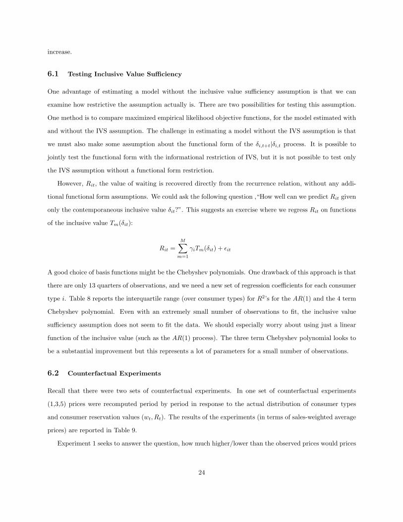
quarter observations. The number of observations still varies from period to period, which can be explained

by two factors. Over time, more FHD (1080p) TV’s and fewer HD TV’s are offered; these trends are displayed

in Table 1. Also, more manufacturers enter the larger size segment over time, which is demonstrated in Table

2.

LCD manufacturers typically assemble televisions from parts purchased from original equipment manu-

facturers (OEM’s). These components include: the panel itself, the power supply, the tuner, and the bezel.

A combination of OEM prices and engineering tear-down analysis makes it possible to estimate the manu-

facturing costs at the panel-quarter level, for example 46” 1080p 120Hz in Q4 2007. An example of this cost

breakdown is presented in Table 3. The most important input, both as a fraction of the cost and as a source

of cost variation is the panel. Panels are produced by upstream panel manufacturers that are independent

of the TV manufacturers.3 In the sample, the panel represents 67% of the cost for the average television,

and represents nearly 80% of the cost variation. The panel makes up a larger portion of the overall costs

for larger televisions (≥ 40”), at 72%, than it does for smaller televisons (< 40”), at only 61%. The share

of panel price over time is plotted in Figure 2. The share of panel price decreases as panels become less

expensive while other input prices remain largely the same (plastic, glass, power supply, etc.). The panel

production process is similar to that of microprocessors (CPUs), in which panels are produced in batches

rather than sequentially and each batch has a failure rate that engineers improve over time. The source of

the decline in panel prices comes from improvements in the yield of the panel manufacturing process, which

is plausibly exogenous.4

An important feature of the market is that panel prices fall sharply during the period of observation.

Steeply falling prices (and costs) are important for understanding the dynamic tradeoffs faced by both con-

sumers and manufacturers. From 2006 to 2009, consumers paid on average 11% less per year for televisions,

and prices of similar televisions fell 17%− 28% per year. Table 4 reports the results of a hedonic regression

of prices on functions of size and resolution. To summarize the results: product characteristics alone explain

about 66% of the price variation in the market, and the addition of a linear time trend increases the R2

3A notable exception is that Sony and Samsung buy most of their panels through S-LCD, a joint venture owned 50-50 bythe two manufacturers.

4It is important to note that the LCD panel manufacturing industry settled one of the largest price-fixing cases of all timein 2006. However, this price fixing behavior was alleged to have taken place back in 2003 and pertained to smaller panels usedin laptop computers, cell phones, and portable music players.

6

to 0.87, while inclusion of manufacturer dummies increases the R2 to 0.92. The regression results imply

that introduction of a new product characteristic (Full HD/1080p resolution) commands a price premium

equivalent to approximately three quarters of price declines. Table 5 reports similar results for marginal

costs, where product characteristics and a time trend explain 97% of cost variation. It is also important

to note that costs fall about 4% per quarter while prices fall almost twice as fast at 8% per quarter (and

on a larger basis) according to the hedonic estimates. This motivates the need for a dynamic model which

explains declining markups and addresses the inter-temporal nature of the consumer’s problem.

3 Demand Model

There is a growing and recent literature on extending models of differentiated products demand (such as

Berry, Levinsohn, and Pakes (1995)) to incorporate consumer dynamics and durable goods. Many of these

approaches exploit a unique property of logit-type models that allows the expected utility of making a

purchase to be written in a closed-form that does not depend on which product is purchased. This literature

begins with Melnikov (2001) and has been employed in a number of studies of the digital camera market

including: Chintagunta and Song (2003), Gowrisankaran and Rysman (2009), Carranza (2007), and Zhao

(2008). This section presents the model of Gowrisankaran and Rysman (2009) and the following subsection

modifies the model to fit the LCD TV industry.

In this model a consumer i with tastes αi who owns good j in period t earns flow utility that depends

on the characteristics of the good (both observable xjt and unobservable ξjt) but not the price pjt:

vijt = xjtαxi + ξjt

In the period of purchase consumers earn the flow utility less the price paid pjt plus an idiosyncratic error

εijt:

uijt = xjtαxi + ξjt − αp

i pjt + εijt or ui0t = vi0t + εi0t

Consumers seek to maximize the present discount value of the stream of flow utilities, and solve the following

dynamic optimization problem:

Vi(εit, vi0t,Ωt) = max

ui0t + βE[EVi(vi0t,Ωt+1)|Ωt],maxj

uijt + βE[EVi(vijt,Ωt+1)|Ωt]

7

In this context Ωt is a state variable that contains all of the relevant information for the consumer’s decision.

The expected utility that consumer i gets from purchasing product j in period t is the flow utility less the

price paid, plus the continuation value associated with owning a product that gives flow utility vijt:

δijt = δij(Ωt) = vijt − αi ln pjt + βE[EVi(vijt,Ωt+1)|Ωt]

When all of the error terms εijt are i.i.d. type I extreme value, then the expected utility of consumer i who

makes any purchase in period t can be written as the logit inclusive value:

δit = δi(Ωt) = ln

∑j

exp[δij(Ωt)]

Following Rust (1987), it is possible to integrate the logit error εijt out of the value function, which simplifies

the expression:

EVi(vi0t,Ωt) = ln (exp(δit) + exp(vi0t + βE[EVi(vi0t,Ωt+1)|Ωt])) + γ

In the above expression EVi(vi0t,Ωt) represents expectation (over ε) of the reservation value of a consumer

i who holds stock vi0t in state Ωt, where γ is the constant term in the utility function. A consumer will not

make a new purchase unless the utility from making such a purchase exceeds the reservation value.

It is important to note that EVi(vi0t,Ωt) only depends on the inclusive value δit and not directly on

prices, product characteristics, or other features of the market. One challenge of dynamic models is that

when the state space is large, they become difficult to solve. In order to avoid this challenge, Melnikov (2001)

and others assume that the reservation value depends only on the current period inclusive value δit. Such

an assumption would imply not only that EVi(vi0t,Ωt) = EVi(vi0t, δit), but also that the evolution of the

state space Pi(Ωt+1|Ωt) = Pi(δt+1|δt).

Assumption 1. Inclusive Value Sufficiency (IVS) (Melnikov 2001) (Gowrisankaran and Rysman 2009)

If δi(Ωt) = δi(Ω′t) then Pi(δi(Ωt+1|Ωt) = Pi(δi(Ω′

t+1|Ω′t) for all t and (Ωt,Ω′

t).

Under this assumption, the value of waiting can be written as a function of the current flow utility, and

the current period inclusive value:

EVi(vi0t, δit) = ln(exp(δit) + exp(vi0t + βE[EVi(vi0t, δi,t+1)|δit])) + γ

8

Then, the probability that consumer i buys good j in period t can be expressed as the product of the

probability that the consumer buys any good in period t and the conditional probability of choosing good j

given some purchase in t:

sijt(vi0t, δijt, δit) =eδit

eEVi(vi0t,δit)−γ· eδijt

eδit

= exp[vijt − αi ln pjt + βE[EVi(vijt, δi,t+1)|δit]− EVi(vi0t, δit) + γ]

In order to close the model, we must specify the beliefs of consumers so that it is possible to calculate

E[EVi(vijt, δi,t+1)|δit]. The literature considers different functional forms for E[δt+1|δt], a common choice is

to parametrize the inclusive value as an AR(1):

δi,t+1 = γ1i + γ2iδit + νit

This functional form assumption can be a bit controversial because this is not the implication of any economic

restriction on the model. While the demand model may indicate that the inclusive value is sufficient for

understanding a consumer’s two period decision, nothing indicates that the inclusive value today is sufficient

for predicting tomorrow’s inclusive value. Also, when considering a model of supply as well as demand, firms

may try to game the functional form of consumer beliefs.

3.1 Restricting Upgrades and Relaxing the IVS Assumption

One of the most challenging aspects in solving the consumer’s dynamic decision problem is keeping track

of the utilities and continuation values for consumers who have already made a purchase. In many mar-

kets, particularly over short periods of time, repeat purchases are rare. Without individual level data on

purchases, ruling out repeat purchases ex ante can substantially simplify the problem. In studying digital

cameras Carranza (2007) and Zhao (2008) ignore repeat purchases, while Gowrisankaran and Rysman (2009)

find keeping track of repeat purchasers is important. As previously indicated, there is little evidence that

consumers replace LCD TV’s from 2006-2009.

When repeat purchases are ruled out, it is without loss to assume that all utility is earned at the time of

purchase (since utility now represents the present discount value of flow utilities 11−β vijt). It is also possible

to normalize the expected utility of the outside good E[ui0t] = 0. This allows us to consider the same

problem as in the previous section, but without the Inclusive Value Sufficiency assumption, so that the state

9

space remains Ωt.

uijt = xjtαxi + ξjt − αp

i pjt + εijt or ui0t = εi0t (1)

Vi(εit,Ωt) = max

εi0t + βE[EVi(Ωt+1)|Ωt],maxj

uijt

(2)

δit = maxj

uijt = ln

∑j

exp[xjtαxi − αp

i pjt + ξjt]

(3)

Consumers now make a purchase when their utility exceeds some reservation utility level. The same trick

from Rust (1987) simplifies the reservation utility by integrating out the εijt terms:

EVi(Ωt) = ln(exp(δit) + exp(βE[EVi(Ωt+1)|Ωt])) (4)

The advantage of eliminating repeat purchases is that the value function is recursive but otherwise depends

only on δit. Moreover, the state space is discrete (since it doesn’t depend on an existing stock vi0t), therefore

it is without loss to treat the relevant state variable as simply the period, so Ωt = t. This suggests a change

of variables for (4):

Rit = EVi(Ωt) (5)

⇒ Ri,t = log (exp(δit) + exp(βE[Ri,t+1|Ωt])) (6)

= log (exp(δit) + exp(βRi,t+1)) + γit (7)

One way to think about γi,t is as an error in the consumer’s calculation of the expected value of period t,

E[EVi(Ωt)]. If consumers have rational expectations, then the error should be orthogonal to the contents

of the consumer’s information set at time t, so that prices, costs, and product characteristics at time t

can all serve as valid instruments. This approach imposes weaker informational restrictions than the IVS

assumption, and does not require any functional form assumptions on Pr(δi,t+1|δit) or Pr(Ωt+1|Ωt). It is

also worth pointing out that Rit is already pinned down in (7) by the logit form without the need for further

restrictions.5

Each type’s market share sijt is the product of the inside share and the purchase probability, where the

purchase probability is now determined by the reservation value Rit. The overall share is the type-weighted

sum of the individual shares, where wit denotes the fraction of households yet to make a purchase who are5If consumers are able to perfectly predict future prices and product quality, then γi,t is zero.

10

of type i in period t:

sijt =eδit

eRit−γit· exjtα

xi +ξjt−αp

i pjt

eδit= exp[xjtα

xi + ξjt − αp

i pjt −Rit + γit] (8)

sjt =∑

i

witsijt (9)

The other important implication of eliminating repeat purchases, is that consumers vanish from the market

after making a purchase. This means that the evolution of the consumer types distribution follows a simple,

deterministic rule:

wi,t+1 = wit(1−∑

j

sijt) (10)

The two dynamic relationships evolve in separate ways, as is indicated in Figure 3. The distribution

of consumer types wt evolves forwards over time; future values of the types distribution depend only the

outside good share and the current distribution of consumer types. The reservation value depends the current

inclusive value and the next period reservation value. The fact that these processes evolve separately, and

in different directions helps to simplify both the estimation and the firms’ pricing problem in the following

sections.6

4 Estimation

The economic model imposes the following constraints:

sijt = exp[xjtαxi − αp

i pjt + ξjt −Rit + γit] (11)

wi,t+1 = wi,t(1−∑

j

sijt) (12)

sjt =∑

i

wi,tsijt (13)

δit = log(∑

j

exp[xjtαxi − αp

i pjt + ξjt]) (14)

Rit = log(exp(δit) + exp(βRi,t+1)) + γit (15)

6The model can be extended to include multiple purchases by expanding the space of consumer types. This can be accom-plished by discretizing consumer inventories vi0t, and the new type space is the product of the existing type space and thespace of consumer inventories. Rather than leave the market after making a purchase, consumers transition to the “type” ofconsumer with the same tastes, but a different inventory holding. This is omitted because it is not an important feature of themarket for LCD televisions.

11

Estimation adds three constraints.7 The first constraint is that the observed shares Sjt match the predicted

shares. The second constraint is that the demand shock ξjt is orthogonal to some function of the observable

variables xjt and the excluded instruments zjt, so that Zjt = [zjt, xjt]. The third constraint is that the error

in the value of waiting is orthogonal to the consumer’s information set at time t.

Sjt = sjt (16)

E[ξjtZjt] = 0 (17)

E[γitf(Ωit)] = 0 (18)

In the presence of over-identifying restrictions, it is not usually possible to solve (17) exactly. Instead,

estimation usually proceeds by choosing an appropriate weight matrix for the moment restrictions and

minimizing a quadratic objective function via Generalized Method of Moments (Hansen 1982).

The empirical likelihood (EL) estimator of Owen (1990) provides an alternative to GMM methods. One

way to think about EL is as an extension of Nonparametric Maximum Likelihood Estimation (NPMLE)

to moment condition models. The empirical likelihood estimator re-interprets the moment condition by

attaching a probability weight to each observation. These weights, ρjt, are constructed so that equation (17)

holds exactly. If each observation in the dataset were distributed as an independent multinomial, then the

corresponding likelihood function would be l(ρ, θ) =∑

∀j,t log ρjt. The resulting optimization problem is to

find a set of weights that maximizes the likelihood subject to the following additional constraints:

∑∀j,t

ρjtξjtZjt = 0 (19)

∑∀j,t

ρjt = 1 (20)

Empirical likelihood estimators provide a number of properties that are desirable to applied researchers.

Many of these properties are related to the fact that EL avoids estimating the weighting matrix. The

estimates derived from EL estimators have the same asymptotic distribution as GMM estimators, but are

higher order efficient (Newey and Smith 2004). The appendix provides more details on the construction

of the EL estimator. Conlon (2009) provides an examination of the computational properties of empirical

likelihood for static demand models, and Kitamura (2006) provides a general survey of the EL literature.

In much of the literature, such as Gowrisankaran and Rysman (2009), Carranza (2007), and Lee (2009),7This formulation of the problem nests the static problem of Berry, Levinsohn, and Pakes (1995). In that problem, wi,t is

fixed, and Rit = 1 + exp[δit].

12

estimation follows a multi-step procedure that involves iterating over three loops. The innermost loop involves

solving a dynamic optimal stopping problem similar to Rust (1987) for the value function. The middle loop

consists of a modified version of the contraction mapping in Berry, Levinsohn, and Pakes (1995) to find

ξjt, and constructing consumer expectations about the evolution of δit. The outer loop involves a nonlinear

search over parameters of a nonlinear (GMM) objective function formed from the moment conditions (17).

Such a method is often quite difficult to implement, and may take several days to achieve convergence.

This paper takes a different approach to estimation, and solves (11) - (20) directly using the MPEC

method of Judd and Su (2008). The key intuition of the MPEC approach is that instead of solving for

equilibrium outcomes at each iteration, these equilibrium outcomes can be viewed as constraints that only

need to hold at the optimum. For example, instead of iteratively solving for the value function for each guess

of the parameters, it is sufficient to ensure that (15) is satisfied at the final estimate θ. The MPEC method

works by using constrained optimization routines to directly solve the system of nonlinear equations implied

by the model. This is markedly different from other approaches in the literature such as: Rust (1987), Hotz

and Miller (1993), Berry, Levinsohn, and Pakes (1995), Aguirregabiria and Mira (2007) which manipulate

equations and solve for parameters as implicit functions of other parameters in order to reduce the number

of parameters and eliminate the contstraints.

It is well established in the literature on optimization (Nocedal and Wright (2006) and Boyd and Van-

denberghe (2008)) that sparse and convex problems are easier to solve than dense and non-convex problems.

Fortunately, (11)-(17) are mostly convex equations8 and reasonably sparse. Sparsity refers to the resulting

Hessian matrix of an optimization problem. It is easy to see that a problem is sparse when many variables

only enter one or two equations (like wit) or enter the model linearly. The “trick” in many MPEC problems

is how to re-write the problem in a way which makes it more sparse. In this case, the “trick” is to replace

the value function with an extra variable, Rit. The difficulty of the MPEC method (and constrained opti-

mization in general) depends more on convexity and sparsity than the number of unknown parameters. As

written, the model implies an extremely large number of parameters (Rit, wit, sijt, δit, ξjt, αi), which would

make it nearly impossible to solve using traditional nested fixed-point methods.

The advantage of the MPEC formulation for the dynamic demand problem is twofold. The first advantage

is that it is substantially easier from a computational perspective. In fact, the dynamic demand problem is8Note: For an optimization problem to be convex, it must have only affine equalities. This problem has several nonlinear

equality constraints, although they are themselves convex. For example, the logit inclusive value: logP

exp(·) is convex (Boyd

and Vandenberghe 2008). The share equation is the ratio of two exponentials evijt

eRit, which are convex, but the ratio is not. This

is not enough to guarantee that the overall optimization is globally convex, and hence has a single unique optimum that canbe found in constant time. However, these equations are well behaved enough that it is usually possible to find the optimumusing off the shelf nonlinear solveers.

13

not appreciably harder than the static demand problem and can be solved in about an hour. One way to see

this relationship is to recognize that the static problem is just the special case of the dynamic problem where

Ri,t+1 = 0 in (15). The second advantage of the MPEC method is that it allows us to define the dynamic

quantities directly as extra variables. Rather than implicitly solving the value function, the dynamic behavior

is just a set of constraints on the (Rit, wit) variables. Moreover, these constraints help exploit the sparsity,

since Rit depends only on the one period ahead value Ri,t+1 and wi,t depends only on the one period lagged

value wi,t. It should be pointed out out that, this system of equations represents an exact solution to the

value function, and does not require approximation on a grid or via polynomials. Additionally, it makes it

possible to estimate the model without additional functional form assumptions on beliefs or the evolution

of the state space, and without assuming that the inclusive value encodes all of the information about a

particular state.

It is helpful to assume that consumers have perfect foresight about the future prices and product charac-

teristics (but not εijt). This allows consumers to solve the dynamic problem implied by (6) exactly so that

γit = 0 ∀i, t. This is restriction is not necessary to estimate the demand model, but it will help simplify the

supply side. From an econometric point of view this may not be such a strong restriction, since Rit and ξjt

both enter the individual share equation sijt. Therefore misspecification in γit should be picked up as part

of ξjt. Insofar as ξjt and γit are interacted with similar sets of instruments, this may not be too restrictive.

Furthermore, robustness tests indicate that the magnitude of γit is typically small.9

9It should not be too difficult to relax this assumption if it turns out to be too restrictive. Although in understanding howfirms set prices, additional assumptions on what is known about γit will need to be made.

14

Under this additional assumption, the overall optimization problem is:

max(ρjt,Rit,wit,sijt,δit,ξjt,αi)

∑j,t

log ρj,t s.t.

sijt =exjtα

xi −αp

i pjt+ξjt

eRit+γit

sjt =∑

i

wi,tsijt

wi,t+1 = wi,t(1−∑

j

sijt)

exp[δit] =∑

j

exp[xjtαxi − αp

i pjt + ξjt])

Rit = log(exp(δit) + exp(βRi,t+1)) + γit

Sjt = sjt∑∀j,t

ρjtξjtZjt = 0

∑∀j,t

ρjt = 1

4.1 Other Estimation Details

In order to estimate this model it is necessary to choose an initial distribution wi0 for consumer tastes αi.

Once the initial distribution is pinned down, the future distribution is determined by the purchase decisions

of consumers. Like in much of the literature, we assume that tastes for individual product characteristics

are independent and normally distributed.10

When we assume that αi are distributed as independent normal random variables, tastes can be broken

up between the population average αk and the individual deviation vik:

αki = αk + σkvik

There are several ways to choose the random tastes and the corresponding population weights (vi, wi0).

The Monte-Carlo approach is to set wi0 = 1ns and then randomly sample vik from the standard normal

distribution. A better method is to choose the draws and weights in accordance with some quadrature

rule. This is particularly effective when the dimension of integration (number of random coefficients) is

low. Theoretically, this approach can be thought about by approximating the function of interest with a

high-order polynomial and then integrating the polynomial exactly. In practice, it simply provides a set of10Over time, as consumers make purchases, the resulting distribution may no longer be normally distributed.

15

points and a set of weights (wi0, vi) in a non-random way. This approach is especially effective for this type

of problem because the integrand sijt is an analytic function, meaning it is well approximated by a Taylor

series, and it is also bounded between [0, 1], which guarantees that the tails die off sufficiently fast.

This paper chooses the initial distribution of consumer types wi0 according to the Sparse-Grids approach

of Smolyak (1963). Heiss and Winschel (2008) determine an efficient way of nesting quadrature rules for ML

estimation of multinomial logit models. The authors find that for three-dimensional logit-normal integrals,

87 quadrature points are more accurate than 2500 quasi-random draws. By using the quadrature points

provided on the authors’ website (http://www.sparse-grids.de), it is possible to accurately approximate a

normal distribution of consumer tastes with a relatively small number of consumer types.

5 Pricing

An important aspect of oligopoly models is that prices are not exogenous, but rather the result of the

profit-maximizing behavior of firms. There is a large literature on static oligopoly models, where inferred

equilibrium behavior of firms is used to recover markups and costs. The idea behind this is that when

observed prices represent equilibrium outcomes of a static differentiated products Bertrand pricing game,

there is a one to one relationship between prices and costs that can be inverted. This relationship is described

in detail in Berry (1994) and Nevo (2000). This paper takes a different approach to the supply-side decisions

of firms. An important feature of the dataset is that marginal cost data are observable, so that costs do not

need to be recovered from the pricing equilibrium.11

Instead, observed costs are used as an input into several counterfactual pricing equilibria. The goal is

to construct counterfactual prices from scenarios where firms consider some aspects of dynamic consumer

behavior but not others. By isolating different aspects of consumer behavior, it is possible to understand

why prices are low (or what would make them higher). We re-compute markups when firms account for

changes in the distribution of types when setting prices, but not consumers’ value of waiting (and vice versa).

Furthermore, it is possible to ask what prices would be in a world where consumers had no option to wait, or

one in which the distribution of consumer types was fixed over time. By comparing prices in these scenarios

to the observed prices (and to the other scenarios) it is possible to measure the extent to which different

types of dynamic behavior influence equilibrium prices.

The next subsection reviews the price setting behavior of a static oligopolist. This provides an important

building block and intuition for some of the counterfactual experiments. The section after that examines11Zhao (2008) develops a novel procedure based on Berry and Pakes (2000) that exploits the orthogonality of the dynamic

pricing Euler equation with some instruments to recover costs without explicitly solving the pricing problem.

16

pricing setting behavior in a dynamic oligopoly setting. Under some simplifying assumptions, and by exploit-

ing the structure of the demand model which lets us separate the value of waiting R from the distribution

of consumer types w, the resulting equilibrium is deterministic and straightforward. The final subsection

applies the static and dynamic equilibrium pricing strategies to different scenarios for consumer behavior.

Static Pricing

It is helpful to define the J×J matrix of same-brand price elasticities, where Jg represents the set of products

owned by multi-product firm g.

Ajk =∂skt

∂pjτwhen (j, k) ∈ Jg, t = τ 0 o.w.

Assume there is a fixed population of consumers M , then firms choose a set of prices pjt for products they

own Jg in order to maximize profits by examining the FOC:

maxpjt∈Jg

πgt = maxpj∈Jg

∑j∈Ag

M(pjt − cjt)sjt(pt, θ)

⇒ sjt =∑k∈Jg

(pkt − ckt)∂skt

∂pjt= A(p− c)

⇒ p = c + A−1s(p, θ)

The extension of this approach to multiple periods is not trivial. At the minimum, oligopolist firms play

a repeated game over several periods, and static Nash-Bertrand is only one possible outcome. Firms can

condition their pricing strategy to depend on actions of other firms. For example, firms may collude in some

periods and engage in price wars in other periods. The dynamic nature of the consumer’s problem makes

this more challenging, since sales in period t depend not only on s(pt, θ, Rt) but also on beliefs about the

future Rt.

5.1 Dynamic Pricing

Firms, subscripted by g, now solve a more challenging problem where σ is a state variable that contains

information about the past history of prices and beliefs by firms and consumers about which strategy is

17

being played.

Vg(σt) = maxpjt∈Ag

Eπgt(σt,pt) + βm

∫Vg(σt+1)Pr(σt+1|σt,pt) (21)

For the demand model in the previous section, if we know the set of consumer tastes and product quality

θ = (ξ, αi), then demand is described in each period by (Rt, wt). In the demand model, Rit is a sufficient

statistic at time t for a consumer’s beliefs about the future. Moreover, both Rt and wt evolve in a simple

deterministic fashion. It is helpful to assume that firms set prices based only on the demand state, and not

explicitly on past actions of other firms. More formally,

Assumption 2. The state variable σ = (Rt, wt, ct) where Rt and wt are the set of all Rit and wit ∀i

respectively and ct is the cost vector for all products j at time t.

Assumption 3. Firms know cjt ∀j, t at time t = 0.

Assumption 3 makes it possible to suppress ct from the state space and instead include it in the t subscript

on the value function. In the LCD TV industry, it is probably reasonable to assume that firms are able to

accurately forecast future costs. This is because costs are driven primarily by panel prices, and panel prices

decline in a predictable way through the engineering process. The hedonic marginal cost regression provides

empirical support for this assumption in Table 5.

Assumption 2 is a stronger assumption, which prevents firms from conditioning their actions on the

actions of other firms, or on the full history of the demand state. This makes it possible to compute pricing

equilibria in a straightforward way, although at the risk of ruling some potentially interesting behavior. Firms

essentially respond to the demand state, and don’t worry about inter-temporal effects of their decisions or

their competitors decisions, except as they influence the demand state.

These assumptions make it possible to simplify the dynamic problem that firms solve in (21) so that:

Vgt(Rt, wt) = maxpjt∈Ag

∑j∈Ag

(pjt − cjt) · sjt(pt, Rt, wt) + βmVg,t+1(Rt+1, wt+1) ∀g, t (22)

wi,t+1 = wi,tsi0t = wi,teδit(pt)

eRit(23)

Ri,t = log (exp(δit(pt) + exp(βRi,t+1)) (24)

The key aspect of this problem is that nothing is stochastic, and the state evolves deterministically in

response to prices. Moreover, the state variables depend on prices only through the exponentiated inclusive

18

value, which has a very simple price derivative, and guarantees that the states are smooth in prices.

∂ exp[δit]∂pjt

= −αpi

∂ exp[δit]∂pjτ

= 0 when τ 6= t

It is possible to construct a sequence of prices, reservation utilities, and a distribution of consumer types

(pt, Rt, wt) that satisfy (22) -(24) and define a Markov Perfect Equilibrium.

If Rit was not affected by the prices firms set in later periods, the distribution of consumer types would

be the only state variable (in addition to costs) and the price setting game in each period t + 1 would be a

strict subgame of the period t game, and an equilibrium could be solved by backward induction. Likewise if

the distribution of consumer types were fixed over time, so that Rit were the only state variable, then the

game in each period t−1 would be a strict subgame of the period t game and an equilibrium could be solved

by forward induction. The intuition behind this is suggested in Figure 3.

5.2 Constructing Counterfactual Pricing Equilibria

The goal of the counterfactual experiments is to understand how prices are affected by different aspects of

dynamic consumer behavior. The advantage of the setup in (22)-(24) is that the value of waiting is captured

by Rit and the distribution of consumer types is captured separately by wit. Therefore, it is possible

to separate out the effect that R and w have on the prices that firms charge. Moreover, the differences

between these two quantities has an economic interpretation. These quantities affect prices in two ways.

The distribution of consumer types wt determines which consumers are left in the market, which enters

demand linearly sjt =∑

i witsijt. The other effect of wit is that firms take into account the effect that prices

today have on the distribution of consumer types tomorrow wi,t+1 through (23). Likewise Rit directly affects

the outside good share today si0t = eδit(pt)

eRit, and future prices determine earlier values of Rit through (24).

These relationships suggest some counterfactual experiments. The goal of the counterfactual experiments

is to understand how much higher (or lower) prices would be if firms did not account for these aspects of

consumer behavior. In order to make this more clear, these aspects are broken out into three parts. The first

part is the dynamic or “indirect” effect. This looks at deviations between a firm that statically set prices

against residual demand each period, and a firm who fully incorporated the effect that prices had on other

periods. Consider the effects of a price increase in period t, it increases the value of the next period t + 1,

since more consumers remain in the market, and it increases the value of the previous period t − 1 since it

makes waiting until period t look less attractive. This leads us to expect that firms which do not account

19

for these dynamic effects will price lower than firms which do. This is addressed in experiments 1 and 2.

The second aspect is that the option value of waiting influences the prices that firms charge. A high value

of waiting means that firms have less ability to extract surplus from consumers. We know from (24) that

a high value of waiting might be due to lower prices or higher quality in the future (through the inclusive

value). We expect that the option to wait should be most valuable when there are substantial changes in

the inclusive value, that is when ∆δit= exp[δit] − β exp[δi,t+1] is large. As an alternative, we can consider

consumers who cannot wait: Ri,t+1 = 0 (or are extremely impatient: β = 0) so that Rit = δit. We can then

compare the prices firms would charge facing these consumers to the observed prices in order to understand

how the option to wait affects prices. This is explored in experiments 3 and 4.

The third aspect is that the distribution of consumer types influences the prices that firms charge. As high

value consumers make purchases, they leave the market and the residual demand curve becomes more elastic

over time. This means that over time, the amount of surplus left in the market should be decreasing.12 As

the amount of potential surplus declines over time, this should lead firms to set lower prices. By comparing

the observed prices to those constructed from a world where the distribution of consumer types does not

change over time (that is consumers who make purchases do not leave the market, but are “reborn” next

period), it is possible to understand the effect that changes in the distribution of consumer types have on

prices. This is explored in experiments 5 and 6.

It is also important to specify which consumers and beliefs firms should face in this counterfactual world.

An option is to consider the initial distribution of consumer types wi0 as a starting point, and to set prices,

the distribution of types, and beliefs (Rit) into motion. This would allow us to simulate a full price path

for the counterfactual world. It allows us to see how prices evolve from period to period in a world with (or

without) some of the dynamic aspects of consumer demand, but makes it difficult to compare to the observed

prices (since they face very different distributions of consumers and beliefs). This approach is explored in

the even numbered counterfactual experiments (2, 4, 6).

The alternative is to consider firms who face the “true” distribution of consumers as implied by the

demand model (Rt, wt) in each period, and see how much higher prices would be period by period. This

lets us explore how firms would set prices against the same population, but where firms differed in their

perceived profit function. It has the advantage that it allows direct comparison with the observed prices,

but the disadvantage that periods are not “linked” to one another. This is explored in the odd numbered

experiments (1,3,5).

12There is a potential source of new “surplus” for firms because marginal costs are also declining over time, but not forconsumers.

20

Experiment 1: Firms do not account for inter-temporal effects when setting prices. Period-

by-Period.

This was the first case described above. This experiment considers the pricing decision where firms correctly

observe the state each period (Rit, wit) but do not take into account how prices affect demand in other

periods. Because this is the period-by-period case, the state (Rit, wit) is taken directly from the demand

model. Markups can be computed using the formula for static markups in (21).

Experiment 2: Firms do not account for inter-temporal effects when setting prices. Full Price

Path.

Just like in Experiment 1, this considers the pricing decision where firms correctly observe the state each

period (Rit, wit) but do not take into account how prices influence demand in other periods. However, in

this experiment, only the initial distribution of types w0 is determined by the demand model. Now, the

reservation values Rit depend on the observed price sequence, and (Rit, wit) are allowed to adjust according

to the demand model. However, firms do not account for their effects on this adjustment. For a given guess of

Rt markups can be computed the same way they are in the static model. The pricing equilibrium is defined

by the system of equations system of equations below, where A represents the proper ownership-elasticity

matrix for (Rt, wt):

pt = ct + At(Rt, wt)−1st(pt, Rt, wt, θ)

wi,t+1 = wi,tsi0t

Ri,t = ln (exp(δit(pt) + exp(βRi,t+1))

Experiment 3: Consumers are myopic. Firms do not account for inter-temporal effects. Period-

by-Period

Consumers are myopic and do not realize that they can make a purchase in a later period. Firms do

not account for how prices affect the distribution of consumer types in the future. Prices are obtained

by modifying (21) so that Ri,t+1 = 0 everywhere. The difference between the prices obtained between

Experiment 3 and Experiment 1 reflects the option value associated with waiting. The distribution of

consumer types wit in each period is obtained directly from the demand model.

Experiment 4: Consumers are myopic. Firms account for inter-temporal effects. Full Price

Path

Consumers are myopic and do not realize that they can make a purchase in a later period so that Ri,t+1 = 0

21

everywhere. The initial distribution of consumers wi0 is used as a starting point and firms set prices in

response to the distribution of consumer types each period. Additionally, when setting prices firms consider

the distribution of consumer types in the future. The resulting pricing equilibrium is subgame perfect and

can be solved by induction.

pt = ct + At(Rt, wt)−1st(pt, 0, w0, θ)

wi,t+1 = wi,tsi0t

The goal of experiments 3 and 4 is to measure how much higher prices would be if consumer were myopic.

The difference in prices between experiment 1 and experiment 3 can be thought about as the a measurement

of the option value of waiting for a period by period case (without dynamic effects). Meanwhile experiment

4 simulates a sequence of prices where the rest of the model dynamics take place, where consumers make

myopic purchase decisions, but leave the market after making a purchase.

Experiment 5: Distribution of Consumer Types is Fixed. Firms do not account for inter-

temporal effects. Period-by-Period

In this experiment the distribution of consumer types is fixed at wi0, but consumers have beliefs about the

future Rit that are obtained by the demand model. Firms set prices each period in response to the observed

Rit and fixed wi0 via the static markup equation in (21).

Experiment 6: Distribution of Consumer Types is Fixed. Firms account for inter-temporal

effects. Full Price Path

In this experiment the distribution of consumer types is fixed at wi0, but consumers have beliefs about the

future Rit that are consistent with the prices set by firms. Firms set prices each period in response to the

(Rit, wi0) and incorporate how prices affect reservation values Rit. Prices are the result of a subgame perfect

equilibrium defined by the following system of equations, and can be solved by induction:

pt = ct + At(Rt, wt)−1st(pt, Rt, w0, θ)

Ri,t = log (exp(δit(pt) + exp(βRi,t+1))

6 Empirical Results

The demand model is estimated via the empirical likelihood method described in a previous section. Three

specifications are reported: a static model similar to Berry, Levinsohn, and Pakes (1995) and the dynamic

22

model with perfect foresight γit. 13.Both specifications are estimated from the same moment condition

E[ξjtzjt] = 0, and the same set of instruments. The instruments are: cost shifters from the marginal cost

data, BLP-style instruments (average characteristics of other brand products in the same market), and non-

price xjt explanatory variables. All models are estimated using the MPEC method and the KNITRO solver,

a modern interior-point solver that handles both constrained and unconstrained problems (Byrd, Nocedal,

and Waltz 2006). As reported in Table 6, the static model implies dramatically different price sensitivities

from the dynamic model, and consumers appear to be far more price sensitive. This bias is well documented

in the empirical literature on dynamic durable goods models, and is due to the fact that the static model

does not account for consumers who do not purchase the good in the current period in order to purchase the

good later. In a comparison of empirical likelihood values (or by constructing the ELR test statistic) we fail

to reject the model without upgrades when compared to the model with upgrades. Thus the model without

upgrades is the preferred specification.

The implied price elasticities and substitution probabilities are reported in Table 7. The first two rows

are the 95% confidence intervals for average own-price elasticities. The average own price elasticity is

E[ ∂sjt

∂pjt], where the expectation is computed over the empirical likelihood probability weights. The 95%

confidence interval is constructed by inverting the χ2 test statistic. Also in Table 7, the following experiment

is conducted, the price of a 32” HD Sony TV in 2008Q1 is increased by 10% from $890 to $980. All

expectations about the future are held constant. That is, Rit is held fixed. This represents a one time

shock akin to a pricing mistake where all retailers mislabel the price of the unit. The table reports how

many consumers substitute to another Sony TV today, how many substitute to the same size and resolution

TV today, how many buy the same Sony unit in the next period, and how many buy some other product

(either now or in the future). The same experiment is repeated for the 32” HD Vizio TV in the same

period where the price is increased from $596 to $655. For both TV’s, few consumers substitute to the same

brand television in a different period, at least when compared with an arbitrary consumer. However, overall

substitution to later periods is quite large. There are two ways to interpret this finding. One interpretation

is that because the market is fairly competitive firms do not compete closely with their own products over

time. The other interpretation is that in the absence of brand specific tastes, and in the presence of a logit

error, we shouldn’t expect strong inter-temporal correlation among tastes for brand. Although the Vizio TV

sells more units than the Sony 240,000 to 170,000, Vizio faces more price sensitive consumers and earns less

of a brand margin, whereas Sony consumers are more likely to stay with the brand in the event of a price13The model without perfect foresight is estimated as a robustness check and gives extremely similar results, and small values

for γit

23

increase.

6.1 Testing Inclusive Value Sufficiency

One advantage of estimating a model without the inclusive value sufficiency assumption is that we can

examine how restrictive the assumption actually is. There are two possibilities for testing this assumption.

One method is to compare maximized empirical likelihood objective functions, for the model estimated with

and without the IVS assumption. The challenge in estimating a model without the IVS assumption is that

we must also make some assumption about the functional form of the δi,t+t|δi,t process. It is possible to

jointly test the functional form with the informational restriction of IVS, but it is not possible to test only

the IVS assumption without a functional form restriction.

However, Rit, the value of waiting is recovered directly from the recurrence relation, without any addi-

tional functional form assumptions. We could ask the following question ,“How well can we predict Rit given

only the contemporaneous inclusive value δit?”. This suggests an exercise where we regress Rit on functions

of the inclusive value Tm(δit):

Rit =M∑

m=1

γiTm(δit) + εit

A good choice of basis functions might be the Chebyshev polynomials. One drawback of this approach is that

there are only 13 quarters of observations, and we need a new set of regression coefficients for each consumer

type i. Table 8 reports the interquartile range (over consumer types) for R2’s for the AR(1) and the 4 term

Chebyshev polynomial. Even with an extremely small number of observations to fit, the inclusive value

sufficiency assumption does not seem to fit the data. We should especially worry about using just a linear

function of the inclusive value (such as the AR(1) process). The three term Chebyshev polynomial looks to

be a substantial improvement but this represents a lot of parameters for a small number of observations.

6.2 Counterfactual Experiments

Recall that there were two sets of counterfactual experiments. In one set of counterfactual experiments

(1,3,5) prices were recomputed period by period in response to the actual distribution of consumer types

and consumer reservation values (wt, Rt). The results of the experiments (in terms of sales-weighted average

prices) are reported in Table 9.

Experiment 1 seeks to answer the question, how much higher/lower than the observed prices would prices

24

be if firms did not account for the inter-temporal effects of pricing decisions. Theory suggests that when firms

do not account for the fact that higher prices improve the profitability both of later periods, because the

number of consumers in the future population increases, and the profitability of earlier periods since higher

prices in the future reduce value of waiting. In the case of experiment 1, the prices are quite similar, but

not always lower than the observed prices. One potential explanation is that the pricing model assumes the

costs are perfectly measured, and there may be unobserved cost variation. Also, the pricing model assumes

away not only the dynamic effects on consumers, but also the dynamic effects on other firms.

Experiment 3 is similar to experiment 1 except that consumers are also myopic, that is Ri,t+1 = 0. This

produces prices that are initially substantially higher (around 30%), but the difference between the predicted

prices and the observed prices declines over time. This makes sense if the consumer’s value of waiting declines

over time. For consumers who prefer small to medium sized televisions, price declines towards the end of

the sample are small, and the value of waiting is declining. Thus the gap between a consumer with no value

of waiting and one who has a declining value of waiting narrows over time.

Experiment 5 is similar to experiment 1 except that while consumers are able to anticipate the future,

the distribution of consumer types is fixed over time. Intuition suggests that firms will sell to high-value

consumers over and over. This is a bit more complicated than the traditional static setting, because costs

fall in each period. In this case, prices fall over time, but fall more quickly early on when costs are also

falling fast. In the later periods when costs are falling more slowly (and there is less incentive to wait) prices

also fall more slowly. Also, unlike in the observed data, prices fall more slowly than costs overall.

Experiments 2,4,6 are presented in Figure 5. These give similar qualitative results to the corresponding

experiments (1,3,5). The major difference is that rather responding period by period, the paths of prices,

reservation values, and the distribution of consumer types are given an initial starting point and then a full

path is simulated over time using the model. It becomes clear that the price discrimination incentive (the

type distribution of consumers) is the dominant factor. The reservation value also has a significant effect on

prices, but only when costs are declining. Meanwhile, it does not appear that firms internalize inter-temporal

effects of prices very strongly. Experiment 2 seems to indicate that firms do not account for the effect of

prices on demand in other periods, or at least that the magnitude is relatively small compared with the

inter-temporal price discrimination and reservation value effects.

When compared to theoretical predictions for the monopoly case, there are some important differences

in oligopoly markets. The distribution of consumer types determines the amount of surplus remaining in

the market, which is not reduced by competition. Counterfactual experiments demonstrate that were it not

25

for changes in the distribution of consumers over time (the price discrimination motive) prices might be

around 50% higher than they are today. Similarly, the option value to wait limits the amount of surplus

firms are able to extract, but so do competitors. In the absence of the option value prices would be only

around 20% higher. Both competition and the logit error may reduce the extent to which firms engage in

inter-temporal competition with their own products. Empirically, firms do not seem to take into account the

effect that prices have on other periods, or these effects are small relative to the other effects, and unlike in

the monopoly case, static pricing does not appear to be bad approximation.

7 Conclusion

This paper adapts the existing methodology for dynamic models of differentiated products to the MPEC

framework. In this framework, dynamic consumer behavior places only a few simple constraints on the

static demand model. This makes it possible to estimate the model directly without making any additional

functional form assumptions or the inclusive value sufficiency assumption. Empirical likelihood estimators

can be adapted quite naturally to the MPEC framework. The resulting estimator is likely to be more efficient,

and easier to compute than standard approaches based on GMM estimators and fixed point algorithms.

In addition to improving the statistical and computational properties, this approach simplifies the eco-

nomics as well. It is possible to estimate the model directly without making additional functional form

assumptions or the inclusive value sufficiency assumption. In industries where repeat purchases are not an

important aspect of consumer demand, it is possible to consider the value of waiting as an additional variable.

When this is the case, it is possible to identify the changes in the distribution of consumer types separately

from the value of waiting. Separating these quantities simplifies the dynamic pricing problem firms face, and

makes it possible to quantify how the value of waiting and changes in the distribution of consumer types

differently effect the prices we observe in equilibrium.

This paper provides a simple framework for beginning to understand the dynamics of supply and demand

in differentiated products oligopoly settings. However, much remains to be done. For example, this approach

does not consider the dynamic effects that firms and prices have on each other (such as collusion, price-fixing,

etc.) though these are often an interesting and important aspect of markets with high-technology products

and fast price declines. Also, the pricing problem uses the simplifying assumption that consumers are able

to exactly predict their expected utility of future states. Likewise, both supply and demand exploit the

assumption that there are no repeat purchases. These assumptions are perhaps reasonable over a short

period of time in the LCD TV industry, but may be more problematic when adapted to other industries.

26

References

Abowd, J. M., and D. Card (1989): “On the Covariance Structure of Earnings and Hours Changes,”Econometrica, 57(2), 411–445.

Ackerberg, D., and M. Rysman (2005): “Unobserved product differentiation in discrete-choice models:estimating price elasticities and welfare effects,” RAND Journal of Economics, 36(4).

Aguirregabiria, V., and P. Mira (2007): “Sequential Estimation of Dynamic Discrete Games,” Econo-metrica, 75(1), 1–53.

Altonji, J. G., and L. M. Segal (1996): “Small-Sample Bias in GMM Estimation of Covariance Struc-tures,” Journal of Business and Economic Statistics, 14(3), 353–366.

Berry, S. (1994): “Estimating discrete-choice models of product differentiation,” RAND Journal of Eco-nomics, 25(2), 242–261.

Berry, S., J. Levinsohn, and A. Pakes (1995): “Automobile Prices in Market Equilibrium,” Economet-rica, 63(4), 841–890.

Berry, S., and A. Pakes (2000): “Estimation from The Optimality Conditions of Dynamic Controls,”Working Paper.

Boyd, S., and L. Vandenberghe (2008): Convex Optimization. Cambridge University Press, 6th editionedn.

Bulow, J. I. (1982): “Durable-Goods Monopolists,” Journal of Political Economy, 90(2), 314.

Byrd, R. H., J. Nocedal, and R. A. Waltz (2006): KNITRO: An Integrated Package for NonlinearOptimizationpp. 35–59. Springer-Verlag.

Carranza, J. (2007): “Demand for durable goods and the dynamics of quality,” Unpublished Mansucript.University of Wisconsin.

Chintagunta, P., and I. Song (2003): “A Micromodel of New Product Adoption with Heterogeneous andForward Looking Consumers: Application to the Digital Camera Category.,” Quantitative Marketing andEconomics, 1(4), 371–407.

Coase, R. (1972): “Durability and Monopoly,” Journal of Law and Economics, 15(1), 143–149.

Conlon, C. (2009): “The MPEC Approach to Empirical Likelihood Estimation of Demand,” UnpublishedMansucript. Yale University.

Dube, J., J. T. Fox, and C.-L. Su (2009): “Improving the numerical performance of BLP static anddynamic demand estimation,” Working Paper.

Erdem, T., S. Imai, and M. Keane (2003): “A Model of Consumer Brand and Quantity Choice Dynamicsunder Price Uncertainty,” Quantitative Marketing and Economics, 1(1), 5–64.

Erickson, T., and A. Pakes (2008): “An Experimental Component Index for the CPI: From AnnualComputer Data to Monthly Data on Other Goods,” Working Paper.

Gowrisankaran, G., and M. Rysman (2009): “Dynamics of Consumer Demand for New Durable Goods,”Working Paper.

Hansen, L. P. (1982): “Large Sample Propertes of Generalized Method of Moments Estimators,” Econo-metrica, 50, 1029–1054.

27

Heiss, F., and V. Winschel (2008): “Likelihood approximation by numerical integration on sparse grids,”Journal of Econometrics, 144(1), 62 – 80.

Hendel, I., and A. Nevo (2007a): “Measuring Implications of Sales and Consumer Inventory Behavior,”Econometrica.

Hendel, I., and A. Nevo (2007b): “Sales and Consumer Inventory,” The RAND Journal of Economics.

Hotz, V. J., and R. A. Miller (1993): “Conditional Choice Probabilities and the Estimation of DynamicModels,” Review of Economic Studies, 60(3), 497–529.

Judd, K. L., and C.-L. Su (2008): “Constrained optimization approaches to estimation of structuralmodels,” Working Paper.

Kitamura, Y. (2006): “Empirical Likelihood Methods in Econometrics: Theory and Practice,” CowlesFoundation Discussion Paper 1569.

Lee, R. S. (2009): “Vertical Integration and Exclusivity in Platform and Two-Sided Markets,” WorkingPaper.

Melnikov, O. (2001): “Demand for Differentiated Products. The case of the US computer printer market.,”Working Paper. Cornell University.

Nair, H. (2007): “Intertemporal Price Discrimination with Forward-looking Consumers: Application to theUS Market for Console Video-Games,” Quantitative Marketing and Economics, 5(3), 239–292.

Nevo, A. (2000): “A Practitioner’s Guide to Estimation of Random Coefficients Logit Models of Demand(including Appendix),” Journal of Economics and Management Strategy, 9(4), 513–548.

Newey, W. K., and R. J. Smith (2004): “Higher Order Properties of GMM and Generalized EmpiricalLikelihood Estimators,” Econometrica, 72(1), 219–255.

Nocedal, J., and S. Wright (2006): Numerical Optimization, Springer Series in Operations Researchand Financial Engineering. Springer, 2nd edn.

Owen, A. (1990): “Empirical Likelihood Ratio Confidence Regions,” The Annals of Statistics, 18(1), 1725–1747.

Pakes, A. (2003): “A Reconsideration of Hedonic Price Indices with an Application to PC’s,” AmericanEconomic Review, 93(5), 1578–1596.

Rust, J. (1987): “Optimal Replacement of GMC Bus Engines: An Empirical Model of Harold Zurcher,”Econometrica, 55(5), 999–1033.

Smolyak, S. (1963): “Quadrature and interpolation forsmulas for tensor products of certain classes offunction,” Soviet Mathematics Doklady, 4, 240–243.

Stokey, N. L. (1982): “Rational expectations and durable goods pricing,” Bell Journal of Economics,12(1), 112–128.

von der Fehr, N.-H. M., and K.-U. Kuhn (1995): “Coase versus Pacman: Who Eats Whom in theDurable-Goods Monopoly?,” Journal of Political Economy, 103(4), 785–812.

Zhao, E. (2008): “Why Are Prices Falling Fast? An Empirical Study of the US Digital Camera Market,”Unpublished Mansucript. Queens College.

28

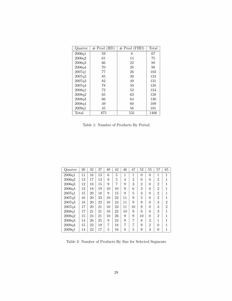
Quarter # Prod (HD) # Prod (FHD) Total2006q1 59 8 672006q2 61 14 752006q3 66 22 882006q4 70 28 982007q1 77 26 1032007q2 85 39 1242007q3 82 49 1312007q4 78 50 1282008q1 72 52 1242008q2 65 63 1282008q3 66 64 1302008q4 49 60 1092009q1 45 56 101Total 875 531 1406

Table 1: Number of Products By Period

Quarter 26 32 37 40 42 46 47 52 55 57 652006q1 11 16 13 6 5 1 1 0 0 1 12006q2 13 17 13 9 5 4 2 0 0 2 12006q3 12 18 15 9 7 9 3 2 0 2 12006q4 12 18 19 10 10 9 6 3 0 2 12007q1 15 20 18 9 15 9 5 3 0 2 12007q2 16 20 23 10 22 11 9 5 0 2 12007q3 18 20 22 10 24 11 9 9 0 3 22007q4 17 20 21 10 23 11 10 9 0 3 22008q1 17 21 21 10 22 10 9 9 0 3 12008q2 15 24 21 10 26 9 9 10 0 2 12008q3 14 26 25 9 24 9 7 8 2 1 12008q4 15 23 19 7 18 7 7 9 2 0 12009q1 14 22 17 5 16 8 5 9 3 0 1

Table 2: Number of Products By Size for Selected Segments

29

Input Q4 2007 Q1 2008LCD Module Price in Previous Quarter 810.31 789.91Inverter 0.00 0.00NTSC Tuner 5.16 0.00ATSC Tuner Demod 21.85 5.40Image Processing 21.38 21.32Audio Processing 10.30 8.60Power 20.02 25.00Other Electronics 29.83 28.48PCB Mechanical 5.76 5.00Other Mechanical 92.24 85.30Packaging&Accessories 16.09 16.04Royalties 10.00 10.00Labor Overhead 62.58 59.70Warranty for 12-18 Months 31.29 29.85USA Import Duty 0.00 0.00Freight to USA 6.52 6.46Insurance 4.57 4.36Handling & Surface 8.04 7.67Ex-Hub 1155.92 1103.09Brand Margin (%) 21% 24%Reseller Margin (%) 25% 27%Average Street Price 1954.16 1976.00

Table 3: Cost Breakdown Example

log(Price) (1) (2) (3) (4)size 0.0519*** 0.0498*** 0.0487*** 0.0496***

(0.0015) (0.00094) (0.00074) (0.00071)

size2 0.000978*** 0.000867*** 0.000749*** 0.000744***(0.00010) (0.000063) (0.000051) (0.000048)

FHD 0.0861*** 0.262*** 0.231*** 0.223***(0.025) (0.016) (0.013) (0.012)

trend -0.0828*** -0.0838*** -0.0890***(0.0018) (0.0014) (0.0022)

Constant 4.936*** 5.577*** 5.519*** 5.585***(0.051) (0.035) (0.039) (0.041)

Fixed Effects x x Manuf Manuf + TimeObservations 1406 1406 1406 1406R2 0.66 0.87 0.92 0.93

Table 4: Hedonic Regression for Prices

30

log(Cost) (1) (2) (3)size 0.0678*** 0.0573*** 0.0551***

(0.0080) (0.0028) (0.0018)

size2 -0.000205** -0.0000959*** -0.0000714***(0.000094) (0.000033) (0.000021)

FHD 0.0427 0.0946*** 0.104***(0.044) (0.015) (0.0097)

trend -0.0379*** -0.0413***(0.00064) (0.0010)

Constant 3.980*** 4.841*** 5.138***(0.16) (0.058) (0.045)

Fixed Effects x x TimeObservations 506 506 506R2 0.74 0.97 0.99

Table 5: Hedonic Regression for Marginal Costs

Static DynamicPrice -.0034 -0.0291FHD 2.2423 1.8412Size -0.0251 0.0184Size2 -.0006 -0.002σp 0.0009 0.0059σs 0.0113 0.00162σFHD 0.0233 0.0621FE Manuf + Q4 Manuf + Q4EL 11438 10941

Table 6: Demand Estimates

Sony 32in HD Vizio 32in HDOwn Elasticity (Lower) -0.83 -0.94Own Elasticity (Upper) -0.61 -0.72Same Model 48% 14%Same Brand-Period 11% 10%Same Period-Other Brand 27% 39%Same Brand-Other Period 4% 6%Other-Other 10% 31%

Table 7: Elasticities and Product Substitution

25th percentile 75th percentileδit only .62 .893 Term Chebyshev .81 .97

Table 8: R2 for Regressions of Rit on f(δit)

31

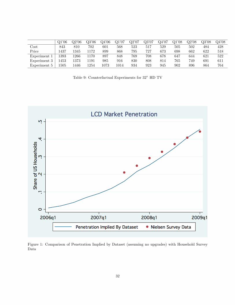
Q1’06 Q2’06 Q3’06 Q4’06 Q1’07 Q2’07 Q3’07 Q4’07 Q1’08 Q2’08 Q3’08 Q4’08Cost 843 810 702 601 568 523 517 529 505 502 484 428Price 1437 1345 1172 899 868 795 727 673 698 662 622 518Experiment 1 1393 1266 1170 897 848 769 708 678 647 644 621 522Experiment 3 1453 1373 1191 985 916 830 808 814 765 749 691 611Experiment 5 1505 1446 1254 1073 1014 934 923 945 902 896 864 764

Table 9: Counterfactual Experiments for 32” HD TV

Figure 1: Comparison of Penetration Implied by Dataset (assuming no upgrades) with Household SurveyData

32

Figure 2: Panel Price as a Share of Overall Costs

33

Figure 3: Timing of Dynamic Problem

34

Figure 4: Empirical Likelihood Confidence Interval Construction

35

Appendix

Static Model

We could imagine a world where in every period consumers choose to purchase the product that gives themthe highest utility, where dit denotes the decision of consumer i in period t and uijt denotes the utilityconsumer i receives from choosing product j in period t. Because utility is ordinal, not cardinal, it isstandard to normalize the mean utility of the outside good to be zero.

dit = arg maxj∈0,Jt

uijt

uijt = αxi xjt − αp

i pjt + ξjt + εijt

ui0t = εi0t

The key addition is the random εijt term, this represents an idiosyncratic shock to the consumer’s utility.There are two ways to understand this, it might incorporate actual shocks to an individual’s utility (it mightfit perfectly in some space, the one the consumer is standing in front of when they make a decision, etc.), orit may be some purely statistical error that provides smoothness. When the random term is Type I ExtremeValue and IID over all (i, j, t) then consumer choice probabilities take on the well known logit form:

sijt =exp[αx

i xjt − αpi pjt + ξjt]

1 +∑

k∈Jtexp[αx

i xkt − αpi pkt + ξkt]

The goal of estimation is typically to identify the distribution of the tastes αi by matching observed sharesto those predicted by the model. We’re typically interested in some parametric distribution f(αi|θ) subjectto the nuisance parameters ξ

sjt =∫

sijt(αi, ξ)f(αi|θ)

There are several problems in using a traditional static differentiated products model to study the purchasesof TV’s. The core problem is that the static model fails to account for the fact that there are tradeoffsbetween purchasing a product today, and waiting until later.

One aspect is that the utility, uijt of buying a product may continue for several periods after the purchaseis made, rather than all enjoyed immediately. We might consider uijt to be the present discount value ofthe flow of future utility from owning the product. But simple adjustments like this are not sufficient.When we consider the outside option 0, as representing “waiting until later”, then it should be clear thatthe assumption E[ui0t] = 0 is incorrect, especially if we know tomorrow’s products will be better and lessexpensive than today’s products, or if a consumer has already purchased a product in the previous period.14

The other problem is that in order to identify f(αi|θ) we typically make the assumption that the distri-bution is constant over time, and use repeated observations of the cross section for identification. This mightbe appropriate for studying durable consumer goods in markets with stable characteristics and prices suchas washing machines or refrigerators where replacement is driven on a fixed interval or by random failures.However, in markets where prices and product characteristics are rapidly evolving, we should worry that theindividuals who purchase the product in early periods when prices are high look markedly different from theindividuals who purchase the product in later periods when prices are low.

Empirical Likelihood MPEC

The typical exposition follows Kitamura (2006), which provides an extensive and accessible survey of theEL literature. Assume data zin

i=1 are distributed IID according to unknown measure µ. The econometric

14One approach in the literature for handling this problem is adding a time trend to the consumer’s utility function. Anexample of this is (CITE). This is ad-hoc at best unless we really believe that consumers are becoming unhappier over time.

36

model gives us some moment conditions. The moment conditions, g(z, θ) ∈ Rq may be scalar valued (q = 1)or vector valued (q > 1).

E[g(zi, θ)] =∫

g(z, θ)dµ = 0, θ ∈ Θ ∈ Rk

We can assume (w.l.o.g.) the existence of a nonparametric (multinomial) (log) likelihood function. Then,we search for a measure (set of probability weights) (p1, . . . , pn) ∈ ∆ within the unit simplex, where eachpi corresponds to weight of each observed zi in the data. These weights are then manipulated so that themoment conditions hold exactly. The empirical likelihood estimator is defined as the solution to the followingoptimization problem:

θEL = arg maxθ,p1,...,pn

lNP (θ) =n∑

i=1

log pi s.t.n∑

i=1

pig(zi, θ) = 0, and (p1, . . . , pn) ∈ ∆

EL offers a different interpretation of moment condition models. While GMM asks, “How close (in a spacedefined by some weight matrix) can I get the moments of my model to match the moments of my data?”;EL asks, “How unusual a draw from the multinomial distribution of data would my data represent if mymoment conditions held exactly?”. EL and GMM produce the same asymptotic distribution. As a limitingcase, in a model without over-identifying restrictions (where the maximized GMM objective is zero), theoptimal weights are the empirical weights 1

n and the EL objective function would be −n log n.EL has a number of advantages that make it attractive to applied researchers. Most of these advantages

are due to the fact that EL avoids estimating the GMM weighting matrix. There is a large literature on whyestimating the weight matrix can be difficult, and when it can lead to problems. An well-known exampleis Altonji and Segal (1996) who show that the optimal weighting matrix used in Abowd and Card (1989)exhibits bias as the number of moments increases and as moments become more correlated. Newey and Smith(2004) provide formal results to show that the source of the bias comes from the correlation of momentswith their Jacobian (especially in the case of endogeneity), and the weighting matrix. They also show thatgeneralized empirical likelihood estimators do not exhibit this bias and are higher-order efficient. Conlon(2009) shows that in Monte-Carlo experiments for the static demand problem of Berry, Levinsohn, and Pakes(1995) EL exhibits less bias and tighter confidence intervals than GMM.

The principal reason that empirical likelihood methods are not more popular, is that they are believedto be computationally difficult relative to GMM. Previous approaches generally focus on the unconstraineddual problem, which is appropriate for solving linear models, but becomes challenging when solving nonlinearmodels:

θEL = arg maxθ∈Θ

lNP (θ) = arg maxθ∈Θ

minλ∈Rq

−n∑

i=1

log(1 + λ′g(zi, θ))

An additional advantage of the MPEC method is that the constrained version of EL is no more difficult toestimate than GMM, and in many cases easier. Conlon (2009) also demonstrates how the MPEC approach ofJudd and Su (2008) and Dube, Fox, and Su (2009) can be combined with the EL estimator and applied to thedemand estimation problem of Berry, Levinsohn, and Pakes (1995). The resulting constrained optimizationproblem can be written as:

arg maxp,ξ,θ,w,R

∑j,t

log pjt s.t.∑j,t

pjtξjtzjt = 0 and Sjt = sjt(ξ, θ) and C(R,w, θ, ξ) = 0 (25)

By combining this objective and constraints with the constraints from the dynamic durable goods problemC(R,w, θ, ξ) = 0 in (11)-(15), we can construct a one-step EL estimator.

One challenge of MPEC based estimators is that it is often difficult to obtain standard errors or constructconfidence intervals. The Empirical Likelihood estimator admits a simple test statistic that can be inverted

37

to construct confidence intervals. This is presented in more detail in the Appendix or in Conlon (2009)

Empirical Likelihood/MPEC Inference

The major disadvantage to the MPEC approach is that unlike traditional nested approaches, it does notfacilitate computation of standard errors. In the example of the static demand estimation problem, it is wellknown that the asymptotic standard errors depend on D = E ∂

∂θ g(zjt, θ) and S = E[g(zjt, θ)g(zjt, θ)′]−1

√n(θ − θ) →d N(0, D′S−1D)

g(zjt, ξ, θ) = ξjt(θ)× zjt

dg

dθ=

∂g

∂θ+

∂g

∂ξ· ∂ξ(θ)

∂θ=

∂ξ(θ)∂θ

× zjt

The problem is that ∂ξ(θ)∂θ is not directly defined in the constrained problem, because ξ does not directly

depend on θ. In the traditional fixed-point/contraction mapping approach this is the gradient of the contrac-tion mapping, but must generally be computed numerically. This presents a problem for MPEC estimators,since it requires implementing and computing a fixed-point/contraction mapping approach as well. This canbe quite challenging when the additional dynamic features of the demand model are included, as it requirescomputing ∇θg = ∂g(zjt,θ)

∂θ along the manifold defined by a number of additional constraints.Judd and Su (2008) recommend a bootstrap procedure for maximum likelihood problems. Dube, Fox,

and Su (2009) do not provide an algorithm for computing standard errors in the MPEC-GMM framework,and implicitly rely on a fixed-point approach, for which they derive an expression for the bias caused bynumerical error in the fixed point.

Empirical Likelihood admits the same form of asymptotic distribution as GMM, where V = D′S−1D,except that D and S are computed under the empirical likelihood weights pjt rather than the empiricalweights 1

n , in order to obtain the higher order efficiency property. Empirical likelihood presents an alternatesolution to this problem, whereby we can use the empirical likelihood ratio test statistic. The ELR teststatistic is computed as follows. Estimate an unrestricted model and compute the corresponding empiricallikelihood lEL(θ). Then estimate a model with a linear restriction on the parameter R(θ) = 0 and call thisl(θ0). Then we can construct the ELR test statistic, where r is the dimension of R.

−2(l(θ0)− l(θEL)) ∼ χ2r

We can directly test for significance using this test statistic. Since the test statistic is just a χ2 with r degreesof freedom we can easily compute the critical value cα for some significance level, and construct a confidenceinterval for θk an element of θ by inverting the test:

[θk, θk] = min θk/ max θk ∈ N(θEL) s.t. l(θ) ≥ l(θEL)− 2cα

We search for the largest and smallest value of the element of interest θk that produces an EL objectivevalue close enough to the unrestricted value. This is demonstrated graphically in Figure 4. This proceduremust be repeated for each parameter for which we want to construct a confidence interval. An advantageis that constructing the confidence interval by inverting the test often has better statistical properties thanconfidence regions constructed from the asymptotic distribution (Kitamura 2006)15.

15I need to track down the correct citation here!

38