NBER WORKING PAPER SERIES

A DYNAMIC MODEL OF SUBPRIME MORTGAGE DEFAULT:ESTIMATION AND POLICY IMPLICATIONS

Patrick BajariChenghuan Sean Chu

Denis NekipelovMinjung Park

Working Paper 18850http://www.nber.org/papers/w18850

NATIONAL BUREAU OF ECONOMIC RESEARCH1050 Massachusetts Avenue

Cambridge, MA 02138February 2013

We would like to thank seminar participants at Stanford GSB, Chicago Booth, Olin Business School,Berkeley ARE and IO fest for valuable comments. The views expressed are those of the authors anddo not necessarily reflect the official positions of the Federal Reserve System or the National Bureauof Economic Research.

NBER working papers are circulated for discussion and comment purposes. They have not been peer-reviewed or been subject to the review by the NBER Board of Directors that accompanies officialNBER publications.

© 2013 by Patrick Bajari, Chenghuan Sean Chu, Denis Nekipelov, and Minjung Park. All rights reserved.Short sections of text, not to exceed two paragraphs, may be quoted without explicit permission providedthat full credit, including © notice, is given to the source.

A Dynamic Model of Subprime Mortgage Default: Estimation and Policy ImplicationsPatrick Bajari, Chenghuan Sean Chu, Denis Nekipelov, and Minjung ParkNBER Working Paper No. 18850February 2013JEL No. C14,C5,G21

ABSTRACT

The increase in defaults in the subprime mortgage market is widely held to be one of the causes behindthe recent financial turmoil. Key issues of policy concern include quantifying the role of various factors,such as home price declines and loosened underwriting standards, in the recent increase in subprimedefaults and predicting the effects of various policy instruments designed to mitigate default. To addressthese questions, we estimate a dynamic structural model of subprime borrowers’default behavior. Weprove that borrowers’time preference is identified in our model and propose an easily implementablesemiparametric plug-in estimator. Our results show that principal writedowns have a significant effecton borrowers’ default behavior and welfare: a uniform 10% reduction in outstanding mortgage balancefor the pool of borrowers in our sample would reduce the overall default probability by 22%, and borrowers’averagewillingness to pay for the principal writedown would be $16,643

Patrick BajariUniversity of Washington331 Savery HallUW Economics Box 353330Seattle, Washington 98195-3330and NBERBajari@uw.edu

Chenghuan Sean ChuFederal Reserve Board of Governors20th Street and Constitution Avenue NWWashington, DC 20551 sean.chu@frb.gov

Denis NekipelovUC, Berkeley530 Evans Hall, #3880Berkeley, CA 94720-3880nekipelov@econ.berkeley.edu

Minjung ParkHaas School of BusinessUC Berkeley545 Student Services Building #1900BerkeleyCA 94720-1900minjungp@gmail.com

1 Introduction

The collapse of the subprime mortgage market and its subsequent role in triggering the current recession

lend special importance to understanding the key drivers behind the increase in defaults. Much of

the debate during the crisis aftermath has centered on the efficacy of various government interventions

designed to reduce default, and whether an expansion in the scope of such programs would be desirable.

The answers to these questions critically depend upon how borrowers’ default behavior would respond to

various incentives.

For example, the Home Affordable Refinance Program (HARP), introduced in 2009, streamlines

refinancing for underwater borrowers with “conforming” loans backed by the government-sponsored en-

terprises (GSEs) Fannie Mae and Freddie Mac. An expansion of the program to nonconforming loans

could reduce the incentive to default by negative-net equity borrowers, but could also potentially become

a liability to the GSEs (and to taxpayers) if the frequency of default after refinancing turns out to be more

common for the expanded eligible pool than anticipated. Similarly, the Home Affordable Modification

Program (HAMP), also introduced in 2009, aims to reduce mortgage payments by delinquent borrow-

ers to no more than 31 percent of monthly income, through a combination of interest rate reductions,

principal writedowns, and loan maturity extensions. Neither HAMP nor its predecessor, Hope for Home-

owners, which was introduced a year earlier and focused exclusively on principal writedowns, has been a

great success, in part due to widespread redefault following mortgage modification.2 Just as important,

policymakers have struggled to understand the limited degree of lenders’ participation in these programs.

Very few lenders have been willing to modify mortgages under HAMP or Hope for Homeowners. Partic-

ipation in HARP has been somewhat greater, but still far less than anticipated. In this paper, we aim

to understand the determinants of borrowers’ default behavior. This will allow policymakers to predict

how borrowers’ default decisions would respond to various features of such programs. The predictions

could then be used as a key input to understanding how those features might affect lenders’ participation

incentives.

In answering these questions, it is critical to recognize that default decisions are inherently dynamic

due to the irreversibility of default and the option value associated with being able to default at some

point in the future. In this context, descriptive analysis does not provide enough information to either

quantify the importance of various factors behind the recent surge in defaults or determine the impact

of implementing policy interventions. Furthermore, failure to take into account how borrowers’ dynamic

incentives are affected by policy interventions could lead to misleading welfare analysis and the adoption

2See, for example, United States Department of Treasury report on “The Effects of Principal Reduc-

tion on HAMP Early Redefault Rates” (2012), available at http://www.treasury.gov/resource-center/economic-

policy/Documents/HAMPPrincipalReductionResearchLong070912FINAL.pdf.

2

of ineffective policies. Therefore, we design a dynamic structural model of subprime borrowers’ default

behavior, estimate it using a unique dataset and use this model for market evaluation and comparative

analysis of a number of proposed policies for mitigating subprime mortgage default.

Our model has four key elements. First, the model is dynamic: borrowers are forward-looking and

respond to current shocks as well as expected future shocks by adjusting their default behavior. Second,

the choice set of the borrowers is discrete, whereby in each period the borrower chooses whether to

default on a loan, to prepay (or refinance) the loan, or to continue making just the regularly scheduled

payments. We consider default to be a terminal action, resulting in the borrower receiving a one-time

“compensation” (or rather, utility loss) and no future utility flows, and the dynamic problem coming

to an end. The assumption that default is terminal has important implications for identification and

estimation of the model. Third, the borrower’s decision problem has a finite horizon, reflecting the fact

that mortgages have a fixed maturity, commonly 30 years. This makes our model different from the

infinite-horizon setup that is more commonly seen in the literature. Fourth, our model is a single-agent

model that abstracts from potential interactions among borrowers. We endow our model with these

features in order to provide a realistic and tractable framework for borrowers’ default decisions. The

resulting model bears some resemblance to that of the dynamic discrete choice literature such as Rust

(1987), Magnac and Thesmar (2002), and Gowrisankaran and Rysman (2012).

Our empirical analysis employs a rich dataset from LoanPerformance, which is uniquely geared toward

addressing our questions due to the level of detail it contains. The data cover the majority of subprime

and Alt-A mortgages3 securitized between 2000 and 2007. The unit of observation is an individual

mortgage observed at a point in time. For each loan, we observe information from the borrower’s loan

application, including the terms of the contract, the appraised value of the property, the loan-to-value

(LTV) ratio, the level of documentation, and the borrower’s credit score at the time of origination. We

also observe the month-by-month stream of payments made by the borrower and whether the mortgage

goes into default or is prepaid. To track movements in home prices, we merge the mortgage data with

zip code level home price indices.

Our empirical approach makes several methodological advances. First, we develop an estimation

procedure for finite horizon optimal decision problem with more than two periods which has not been

done before and is conceptually very different from estimation of infinite horizon problems. Such problems

must take into account the nonstationarity of the optimal decision rules due to the presence of a final

period. Our estimation method has a multi-step structure, as in Hotz and Miller (1993). Our estimation

3Alt-A’s are mortgages that are considered riskier than prime but less risky than subprime. In this paper, we casually

use the term “subprime market” to refer to both subprime and Alt-A mortgages. The distinction between the two is in any

case somewhat artificial.

3

method is intuitive and based on iterated application of a linear (or nonlinear) projection. There are two

main advantages to our approach. From the technical perspective, our method does not require forward

simulation and only requires us to make one-period-ahead predictions of borrowers’ decisions, making

it easy to implement using standard statistical software such as STATA. From the conceptual economic

perspective, we do not require the borrowers to form precise long-term forecasts for the transition of state

variables: our setup only requires that borrowers can form one-period-ahead expectations regarding the

state variables and that their preferences be stable. Furthermore, we nonparametrically estimate one-

period-ahead expectations and use the estimates to recover economic agents’ preferences. This approach is

closely related to work in Ahn and Manski (1993), and thus conceptually our approach can be considered

as extending Manski (1991), Manski (1993) and Manski (2000), which examine responses of economic

agents to their expectations in models with uncertainty or endogenous social effects, to the case where the

problem of the economic agent is dynamic. Our approach also conveniently accommodates the limitations

of our data: it circumvents the problems posed by the lack of observations close to the final period, which

characterizes our data because subprime mortgages were only introduced in recent years.

Our second methodological contribution consists of some new results on the (semiparametric) identi-

fication of finite-horizon dynamic discrete decision problems. One of the most interesting results pertains

to identification of borrowers’ time preferences. Identification of the discount factor comes from the fact

that time to loan maturity influences ex ante value functions but does not have any impact on period

utility. Instead of assuming an arbitrary number for the discount factor, as is typically done in the

literature, we present an estimate of time preferences of subprime mortgage borrowers.

Our structural estimates provide a clue to understanding the relative importance of different drivers

of default as well as the potential effects of several broad classes of policy interventions for mitigating

default. To obtain the answer we use the estimated optimal decision rules of borrowers to analyze their

behavior under various “counterfactual” regimes. Our approach differs from the standard approach,

which is to compute the counterfactual outcomes by re-solving for the optimal behavior using estimates

of the structural parameters.4 The usual argument for re-solving for the optimal behavior is to address

the Lucas critique. However, the individual-level panel structure of our data allows us to avoid the

Lucas critique as long as we judiciously choose our counterfactual scenarios. Because the panel structure

allows us to identify the individual optimal decision rules over a very wide range of state variables, so

long as a policy intervention results in state-variable realizations that are actually observed for a subset

of borrowers in the data (i.e., the realizations remain within sample) and does not change the state

4We decided to take this approach mainly due to the data constraint posed by lack of observations for loans close to

maturity. In order to re-solve for the optimal behavior, we must use backward induction starting from the last period of loan

maturity. Because our estimates of the utility function are based on data from more recently originated loans, we would

need to assume that the estimated period utility function from younger loans also applies to loans in their final period, an

assumption we believe to be too strong as discussed in Section 3.

4

transition process (or borrowers’ expectation about it), the new optimal behavior is correctly captured

by the estimated decision rules of borrowers.

As we might expect, the downside of this approach is that it cannot be used to analyze scenarios

involving transitions to states not spanned by the estimation sample or resulting in changes to the state

transitions themselves. Nevertheless, we illustrate that there are many interesting scenarios that can be

fruitfully explored without re-solving for the new optimal behavior. For example, we are able to study

the effects of interventions that boost housing prices, so long as the resulting housing price evolution is

observed in some geographic area within the actual sample. This is not a restrictive assumption, given the

wide diversity of housing price evolution paths in different metropolitan areas. Also, policymakers have

proposed a variety of interventions at the level of individual mortgages, including subsidies for lenders

to forgive mortgage principal and caps on permissible loan-to-value ratios. We can study the effects of

most of these interventions so long as the features of a counterfactual mortgage are within the empirical

support of our data.5 This approach is computationally much lighter than having to re-solve for the new

optimal behavior using backward induction.

We examine the effect of each counterfactual scenario on default behavior. Using the structural

estimates, we also determine welfare consequences for the borrowers. In particular, we compute the

one-time income compensation that is necessary to bring borrowers’ ex ante value function under the

counterfactual scenario back to its original level, which is a measure of compensating variation in our

dynamic setting. For instance, our results show that a uniform 10% reduction in outstanding mortgage

balance for the pool of borrowers in our sample would reduce the overall default probability by 22%, and

that borrowers’ average willingness to pay for the principal writedown would be $16,643.

This paper contributes to the literature analyzing the mortgage market by estimating a fully dynamic,

structural model of borrower behavior. Most of existing empirical work on mortgage defaults uses a

duration framework (Deng, Quigley and van Order (2000); Foster and Van Order (1984); Tracy and

Wright (2012)), which does not take into account the impact of current actions on future payoffs or the

impact of expectations about the future on current actions. The prior literature has established the

importance of considering consumers’ forward-looking behavior in credit and insurance markets more

generally (Einav, Jenkins and Levin (2012); Aron-Dine et al. (2012); Einav et al. (2013)). Estimating

a dynamic structural model informs our understanding of borrowers’ default incentives, and allows us

to evaluate welfare effects of key policy tools, a topic of immense interest to policymakers. The paper

also adds to the growing list of research on the subprime mortgage crisis, such as Foote et al. (2008),

Demyanyk and van Hemert (2011), Keys et al. (2010), Gerardi et al. (2008), and Bajari, Chu and Park

5As a counterexample, we cannot study loan modifications that extend the duration of the loan to lengths not observed

in the sample, such as from 30 years to 45 years.

5

(2011) among others.

In addition, the paper makes a contribution to the literature on identification of time preferences

(Magnac and Thesmar (2002); Fang and Wang (2012)) by proving identification of the discount factor in

our finite horizon model even when researchers do not have data on the final period. Unlike our paper,

most of the prior literature that estimates time preferences relies on experimental data (see Frederick,

Loewenstein and O’Donohue (2002) for a review of the literature).6

The rest of this paper proceeds as follows. In Section 2, we describe the data. In Section 3, we present

our model and discuss identification of the model primitives, including the discount factor. Section 4

discusses our estimation methodology and its sampling properties. Section 5 presents estimation results.

In Section 6, we discuss our counterfactual exercises and welfare implications for borrowers. Section 7

concludes.

2 Data

We use data from LoanPerformance on subprime and Alt-A mortgages that were originated between

January 2000 and September 2007 and securitized in the private-label (i.e., non-GSE) market. The data

cover more than 85% of all securitized subprime and Alt-A mortgages.

For each loan, we observe the loan terms and borrower characteristics reported at the time of origi-

nation, such as the type of mortgage (fixed rate, adjustable rate, etc.), the initial contract interest rate,

the level of documentation (full, low, or none7), the appraised value of the property, the LTV ratio, the

location of the property by zip code, and the borrower’s FICO score.

We focus on 30-year fixed-rate mortgages, the most common mortgage type. We further restrict our

sample to loans that are first liens and that are for properties located in 20 major Metropolitan Statistical

Areas (MSAs).8 We also exclude “cash-out” refinance loans9 from our sample and focus on loans that

are for home purchases or refinances with no cash out. Many homeowners use cash-out refinance loans

for debt consolidation or home improvement, which would significantly change their non-housing-debts

6A few exceptions are Hausman (1979), Yao et al. (2012), and Chung, Steenburgh, and Sudhir (2011).7Full documentation indicates that the borrower’s income and assets have been verified. For low documentation loans,

only certain information about assets has been verified. No documentation indicates there has been no verification of

information about either income or assets.8Atlanta, Boston, Charlotte, Chicago, Cleveland, Dallas, Denver, Detroit, Las Vegas, Los Angeles, Miami, Minneapolis,

New York, Phoenix, Portland, San Diego, San Francisco, Seattle, Tampa, and Washington D.C.9That is, when the borrower takes out a larger loan than needed to pay off the old loan. Our data identify individual

loans and not the identities of borrowers, so we cannot identify the previous loan taken out by a particular borrower.

However, the data identify whether the purpose of each loan was for a home purchase or a refinance, and whether cash was

taken out on a refinance.

6

or home value in a way we do not observe in the data. This makes our model less suitable for explaining

the default behavior of borrowers with cash-out refinance loans.

We do not directly observe the borrower’s income. Instead, we impute it based on the front-end

debt-to-income ratio reported at the time of loan origination, and use it to proxy for the borrower’s

current income during each time period over the course of the loan.10 The front-end debt-to-income

ratio is available for only a very small fraction (3.5%) of all loans, significantly reducing our estimation

sample. In earlier work (Bajari, Chu and Park (2011)) we found that this sample restriction did not

affect key findings on borrowers’ default behavior. Furthermore, even with this restriction, we still have

about 12,000 borrowers in the sample. Hence, we use this sample in our empirical investigation. For

more detailed discussions of the LoanPerformance data, see Demyanyk and van Hemert (2011) and Keys

et al. (2010).

The data track each loan over the course of its life, reporting the outstanding balance, delinquency

status, and scheduled payment in each month. We define default as occurring if the bank takes possession

of the home or if the loan has been delinquent for 90 days or more, a commonly used definition of default

in the mortgage literature. Default is a terminal event, so if a loan defaults in month , it drops from

the sample starting at + 1. We define prepayment as occurring if the loan balance is observed going to

zero before maturity, presumably because the borrower has paid off the loan in full. We do not observe

the new loan used to refinance the original loan, because our data identify individual loans but not the

identities of specific borrowers. When the borrower prepays, we assume that the borrower refinances into

a new loan.11 We assume that the new loan matures at the same maturity date as the old loan and has

an interest rate equal to the current market interest rate.12 13 If the borrower does not default or prepay

in month , the borrower continues to make just the regularly scheduled payment, and the loan survives

into the next month. We track the status of each loan in our sample through December 2009. Thus, we

have data on default behavior for only up through the first ten years of each loan, although the loans

have a maturity of 30 years, an issue we will return to later.

10We approximate the borrower’s income by dividing the scheduled monthly payment by the front-end debt-to-income

ratio, as reported at origination. The front-end ratio measures housing-related principal and interest payments, taxes, and

insurance as a percentage of monthly income. The assumption that household income stays constant over time is a necessary

approximation, given that we only have data on each borrower’s circumstances at the time of origination.11 In practice, some borrowers may prepay because they have sold the house. From the data, we cannot distinguish

between prepayments due to refinancing and prepayments due to home sales. It is our understanding that most subprime

borrowers prepay in order to refinance into a new loan with lower interest rates.12For example, if the borrower refinances when the loan is 50 months old, we assume that the new loan will mature in

310 months. In practice, borrowers typically refinance into a mortgage with a standardized maturity such as 30 years or 15

years. Since some people refinance into 15-year mortgages while others refinance into 30-year mortgages, our assumption is

a reasonable approximation of the average outcome.13We assume that the market interest rate available to borrower at time is equal to = () + , where ()

is the prevailing rate available at time for loans with observable characteristics , and is a borrower-specific spread

that is constant over time. For a given borrower, we can identify as the residual from regressing the observed interest

rate on the observed characteristics of the borrower’s original loan.

7

As a proxy for any potential disruptions in household income over the course of the loan, we use the

unemployment rate at the county level. Data on monthly county-level unemployment rates come from

the Bureau of Labor Statistics. If we observed individual employment status in every month, we would

be able to identify defaults that occur due to income shocks. However, we are limited in our ability to

do so due to the noisiness of our county-level proxy.

To track movements in home prices, we use housing price indices (HPI) at the zip code level, also

from LoanPerformance. LoanPerformance reports the home price indices at a monthly frequency, and

constructs them using the transaction prices of properties that undergo repeat sales at different points

in time in a given zip code area. We impute the current value of a home by adjusting its appraised

value at the time of origination by the index. Because home price declines are thought to be one of

the main drivers behind the recent surge in mortgage defaults, and because there is a high degree of

variation in home price movements across locations even within the same MSA, it is important to have

home price data at a fine geographic level. Hence, we believe that the use of the zip code level HPI from

LoanPerformance enhances the robustness of our results. By contrast, most previous studies on mortgages

and housing markets in general have used the HPI from Case-Shiller, which is only at the MSA level. See

Table 1 for variable definitions.

[Table 1 about here]

Table 2 reports summary statistics, both for the entire sample and separately according to the mode

by which loans come to an end in the sample–by prepayment, by default, or by censoring at the end of

the sample. Maturation is not a relevant category for our sample. As shown, default is associated with

lower income borrowers and lower credit scores. For instance, the average FICO score among all loans is

672.6, compared with an average of 626.4 conditional on default.

[Table 2 about here]

The second panel of Table 2 presents summary statistics for time-varying variables as of the last

period in which we observe each loan. Relative to the overall average across all borrowers, borrowers who

default tend to have less net equity and lower housing value at the point of default. For instance, the

amount of net equity in the last observed period is on average $103,000 among all borrowers, but only

$38,000 for loans that default.

Table 2 also reports the share of loans for home purchases as opposed to no-cash-out refinances, as well

as the share of loans to borrowers who intend to live in the house (owner-occupiers) versus people who

8

buy the house for investment purposes (investors). These partitions of borrowers will become important

later when we discuss borrower heterogeneity.

Table 3 shows that loan characteristics differ significantly across origination years. If loans of different

vintages do not systematically differ from each other and home price transitions are uniform over time,

we would expect that the fraction of loans that default by December 2009 (the end of the sample period)

should be monotonically decreasing as we move to the right in Table 3, because loans from earlier

vintages have had more time over which to default. Instead, we see that the fraction of loans that default

by December 2009 is much higher for loans from the 2005—2007 vintages compared with loans originated

in 2000—2004, suggesting that the later loans were riskier. This difference can be partly explained by

differences in observable loan characteristics and by the decline in home prices in later years. However,

loan characteristics and home price transitions might not fully explain the differences across origination

years, as researchers have found that loans originated in the later years have a higher propensity to

default even after controlling for these factors (Demyanyk and van Hemert (2011)). To account for any

systematic differences in unobservable characteristics, we include origination year dummies in the state

vector.

[Table 3 about here]

Table 4 reports the empirical distribution of the time to default, conditional on a loan eventually de-

faulting (upper panel), and the empirical distribution of the time to prepayment for loans that eventually

prepay (lower panel). Both distributions have a hump shape. A similar hump shape in the default haz-

ard and prepayment hazard is also well-documented in the mortgage literature14 (Gerardi et al. (2008);

von Furstenberg (1969)), but there is no agreement in the literature on what economic forces lead to

the initial increase in default hazard. It could be generated by borrowers’ stronger determination to

make payments on loans that they have just obtained (due to some behavioral biases, for instance) or

by greater uncertainty about income or employment shocks further into the future (e.g., conditional on

a lender approving a loan, presumably the borrower has a steady income in most cases. An unexpected

income shock is thus likelier 18 months down the road as opposed to just after origination). In one of

the alternative specifications we examine below, we modify our analysis to address the impact of such

time-varying unobserved factors on our results.

[Table 4 about here]

14This effect is also confirmed by unreported regressions using our data. All unreported results are available upon request.

9

While many of the state variables listed in Table 1 are time-invariant, three of them–home value,

market interest rate and unemployment rate–stochastically evolve over time.15 These state variables are

nonstationary (based on an independent analysis of their time series behavior), but we can estimate their

transition paths in terms of the growth rate in home value and the first differences in market interest

rate and unemployment rate, which are stationary.

Our analysis assumes that the regulatory regime remained constant over the sample period. In

particular, we assume that borrowers do not experience or expect changes to their mortgages due to

various foreclosure mitigation programs that the United States government implemented in the later

stages of the housing crisis. Two major programs would conceivably be relevant to loans resembling those

in our sample. Hope for Homeowners (based on legislation in Spring 2008) is a principal writedown policy.

Due to lenders’ apparent unwillingness to reduce principal, there has been virtually no participation in

the program. The Home Affordable Modification Program (HAMP, based on legislation in 2009) is a

payment-reduction program. However, most institutions started their HAMP trials in late 2009, largely

after our sample period.16 Furthermore, since these programs have had extremely low take-up rates, it

is a reasonable approximation to assume that borrowers did not expect to benefit from participation in

such programs.

3 Model of Borrowers’ Behavior

We formalize borrowers’ decision process using a dynamic, discrete-time, single-agent model. Each agent

enters a mortgage contract lasting time periods, and solves a dynamic programming problem with a

finite time horizon ending at . The components of the model are as follows.

3.1 Actions

At each time period over the life of borrower ’s loan, the borrower chooses an action from the

finite set = 0 1 2.17 The possible actions in are to default ( = 0), to prepay the mortgage

( = 1), or to make just the regularly scheduled payment for the current time period, which we refer to

15Net equity also stochastically evolves over time. Its evolution is determined by the evolution of home value and

the evolution of the outstanding loan principal. Because the outstanding principal follows a deterministic evolution fully

specified by the contractual interest rate (fixed over time) and loan maturity (also fixed over time), estimating the evolution

of home value is sufficient to infer the evolution of net equity.16A third program, the Home Affordable Refinance Program (HARP, based on legislation in 2009), makes it easier for

borrowers to refinance, but is irrelevant to the subprime loans in our sample because it only applies to loans guaranteed by

GSEs.17Note that we use to denote the loan’s age, not calendar time. A 36-month old loan will have = 36 whether the

loan was originated in January 2003 or October 2007. In our estimation, we limit our attention to all loans with the same

maturity (30 years), so loans with the same have the same number of months remaining until maturity.

10

as “paying” ( = 2). We assume that there is no interaction among borrowers affecting their payoffs,

so our setup is a single-agent model, not a game. We assume that default is a terminal action: once a

borrower defaults, there is no further decision to be made and no further flow of utility starting from the

next period.

3.2 Period Utility and State Transition

Each borrower observes a vector of state variables ∈ S in each period. The support S is a productspace that is a subset of -dimensional Euclidean space. We allow the subspaces of this product space to

be either continuous or discrete. The state vector includes borrower ’s characteristics, the current

home value, monthly payments, etc. We also allow this vector to contain lags of the current period’s

observable state variables. is fully observed by the econometrician. We assume that the borrower

is also characterized by a time-invariant “type” ∈ C (observed by the econometrician) and a time-dependent vector of idiosyncratic shocks associated with each action = (0 1 2) (unobserved

by the econometrician). The set C is assumed to be finite. Although certain elements of may alsobe time-invariant, the purpose of defining a separate type space C will become apparent in Section 4where we discuss our utility specification with random coefficients. Each element of is assumed to

have a continuous support on the real line. We make the following assumption regarding the marginal

distributions of the random variables.

ASSUMPTION 1

(i) Conditional independence of the idiosyncratic payoff shocks: ⊥ | .

(ii) Conditional independence over time of idiosyncratic payoff shocks: | −1 −1 ∼ | −1 .

(iii) Exclusion restriction ( cannot be represented as a linear combination of the elements of ): Cdoes not belong to any proper linear subspace of S.

(iv) Markov transition of the state variables: follows a reversible Markov process, conditional on

.

In our empirical analysis we use a conventional specification of the distribution of the idiosyncratic

shocks, assuming that components of are mutually independent, have a type I extreme value distri-

bution, and are i.i.d. across borrowers and over time. However, this assumption is not essential, and

we establish the existence of an optimal strategy and prove our identification results for an arbitrary

continuous distribution of random shocks that satisfy Assumption 1.

11

Among the state variables, the monthly payment due and the contractual interest rate are the only

ones whose transition is influenced by . As mentioned in Section 2, we assume that when a borrower

prepays in period , he refinances into a new loan that matures at the same time as the old loan and

whose contractual interest rate is equal to the current market interest rate. Thus, the payment level

and contractual interest rate will depend upon the borrower’s choice. We allow the state variables to

follow a high-order Markov process by including the lagged state variables from the previous periods into

the vector . This structure allows us to provide a more realistic empirical model for important state

variables such as the housing prices, which exhibit lag dependence.

We assume that the per-period utility of the borrower is separable in the idiosyncratic shock compo-

nent. We can characterize the borrower’s utility as:

( ; ) = ( ; ) + for

( ; ) = ( ; ) + for =

As specified, the per-period utility has a deterministic component, (· ·; ·), which is a time-invariantfunction of the action, state, and the borrower’s type. The payoff function in the final period can in

general differ from that of earlier periods, capturing the fact that the borrower obtains full ownership of

the house once the mortgage is fully paid off at maturity, which we can think of as adding a lump-sum

boost to the period utility in the final period. Therefore, (· ·; ·) may generally differ from (· ·; ·).

As we demonstrate later in this section, normalization of the per-period payoff of one of the actions,

typically required in discrete choice models, is not innocuous in dynamic discrete choice models like ours.

Thus, we need to normalize the utility from one of the actions in a way that reflects economic conditions

faced by the agents.18

3.3 Decision Rule and Value Function

We consider the borrower’s problem as an optimal stopping problem, and assume that the default decision

is irreversible and that the borrower cannot “re-start” borrowing after default. This assumption is realistic

because default usually so damages a borrower’s credit that borrowing for another house is impossible for

a long time. And even if this were not the case, we could still interpret the borrower’s dynamic decision

problem as being over the timing of payment and default on a mortgage taken out on a particular house:

18 It turns out that the observed decisions fully characterize the utilities from all choices and thus no normalization is

necessary if (a) (· ·; ·) = (· ·; ·) (i.e., the final period’s utility function is the same as the utility function of earlierperiods) and (b) the actions in the final period are observed for some of the borrowers in addition to the actions from earlier

periods. Although these conditions do not apply to our empirical setup, there may be finite-horizon dynamic problems in

other economic settings in which these two conditions are naturally satisfied. Thus, we consider such scenarios as a separate

case in our identification discussions below.

12

default would entail loss of the house, and the assumption of irreversibility would imply that the borrower

cannot reacquire the same house following default. Provided that the default (“stopping”) decision is

irreversible, the choice of the default option is equivalent to taking a one-time “compensation” (more

specifically, a utility loss) without future utility flows. If the borrower pays or refinances his mortgage, he

receives the corresponding period payoff (which is a combination of utility from consumption of housing

services and disutility from payments for the mortgage) plus the expected discounted stream of future

utility. Parameter is the discount factor that characterizes the time impatience of the borrower.

The borrower’s decision rule for each period is a mapping from the vector of payoff-relevant vari-

ables into actions, : S×C×R3 7→ . We denote the borrower’s decision probabilities by (| ) =£1( ) =

¯

¤for ∈ . We collect (| ) for all and such that ( ) =

[( = 0| ) ( = 1| ) ( = 2| )] and = (1(1 ) ( )) , and refer to as the policy function.

Considering the expected discounted sum of utility of the borrower who has not defaulted prior to

period , we introduce the ex ante value function:

(; ) = ()

"X=

µ−( ; )

−1Π

1=11(1 0)

¶|

#

where () represents the state transitions. The term−1Π

1=11(1 0) reflects that once a borrower

defaults, there is no further flow of utility starting from the next period.

The choice-specific value function, denoted by ( = ; ), corresponds to the deterministic

component of the discounted sum of payoffs that the borrower receives when choosing action in period

:

( = ; ) = ( = ; ) + [+1(+1; )| = ] for

( = ; ) = ( = ; ) for =

In particular, the choice-specific value of default is equal to the period utility of default, i.e., ( =

0 ; ) = ( = 0 ; ) for , because default is a terminal action, which makes the future

value term [+1(+1; )| = 0] zero.

13

3.4 Optimal Policy Functions

In the following theorem, we establish a formal existence and uniqueness result characterizing the bor-

rower’s optimal decision.

Theorem 1 Under Assumption 1 there exists a unique decision rule ∗ ( ) supported on for

= 1 2 that solves the maximization problem

sup(12 )∈

1(1; )

Proof. Our argument uses backward induction. In the last period (at the mortgage maturity) the

borrower faces a static optimization problem of choosing among (0 ; ) + 0 , (1 ; ) +

1 , and (2 ; )+2 . The optimal decision delivers the highest payoff, yielding the decision rule

∗ ( ) = argmax∈ ( ; ) + . Provided that the payoff shocks are idiosyncraticand have a continuous distribution, the optimal choice probabilities are characterized by continuous

functions of ( ( ; ) ∈ ). Knowing the optimal decision rule in period , we can obtain the

choice-specific value function in period − 1 as

−1( −1; ) = ( −1; )+∙ P0∈

1∗ = 0 ( (0 ; ) + 0 )¯−1 −1 =

¸

Provided that the period optimal decision is already derived, the optimal decision problem in period

− 1 becomes a static problem of choice among three alternatives. Its solution, again, trivially exists

and is (almost surely) unique because the distribution of −1 is continuous. We iterate this procedure

back to = 1.

If we specify that the distribution of idiosyncratic shocks has the standard type I extreme value

distribution, then it is possible to express the probabilities of default, prepayment, and payment at a

given state, type, and period ≤ in closed form, in terms of the choice-specific value functions and

using the multinomial logit formulas. We can also obtain explicit expressions for the differences between

choice-specific values for different actions in terms of (the logarithms of) the optimal choice probabilities

via the Hotz-Miller inversion.19

In our model, we can identify the levels of the choice-specific values themselves, and not just the

differences, because default is a terminal action, pegging the choice-specific value of default to a fixed

function ( = 0 ; ). The easiest example to illustrate this is when the payoff from the default

19From here on we shall consider only the value functions and choice probabilities corresponding to the optimal decision

rule, so we shall omit the subscript .

14

option is trivially normalized to zero, that is, ( = 0 ; ) = 0 In this case we can recover the

choice-specific value functions and the ex ante value function directly from the data. As we show below,

our model is identified from the data as long as the payoff from default is set to a fixed function.

3.5 (Semiparametric) Identification

In this section we demonstrate that our model is identified from objects observed in the data, namely,

the choice probability of each option, conditional on the current state and the borrower’s observable

type (( = | )); and the transition distribution for the state variables, characterized by theconditional cdf ( |−1 −1).

The model’s three structural elements are: (1) the deterministic component of the per-period payoff

function, (· ·; ·)20; (2) the time preference parameter ; and (3) the conditional distribution of theidiosyncratic utility shocks to the borrowers, which have the type-specific joint cdf (·|). We shallargue that (· ·; ·) is nonparametrically identified and that the time preference parameter is identified,for a given distribution of the idiosyncratic payoff shocks satisfying Assumption 1. We emphasize that

our identification results do not rely on the extreme value assumption regarding the distribution of the

idiosyncratic shocks.

We show the model is identified by demonstrating that there exists a unique mapping from the

observable distribution of the data to the structural parameters. We start with the case in which the

payoff from the default option is known, and then consider relaxing this assumption.

Theorem 2 (Identification with fixed, known default utility) Suppose that the payoff from the

default option is a fixed, known function (0 ·; ), and that the distribution of idiosyncratic shocks condi-tional on the borrower-specific heterogeneity variables , (·|), has a full support with the density strictlypositive on R3. Also, suppose that for at least two consecutive periods and 0 (·; ·) 6= 0(·; ·) for ∈ .

(i) If the data distribution contains information on at least two consecutive periods and the discount

factor is fixed, the per-period utility (· ·; ·) is nonparametrically identified. Moreover, if (· ·; ·) = (· ·; ·) and one of the observed periods is the period of mortgage maturity , then the discount

factor is also identified.

(ii) If the data distribution contains information on at least three consecutive periods, then both the

20We omit discussion regarding identification of (· ·; ·), as it is obvious that (· ·; ·), in case 6= , is identified if

and only if decisions from the final period are observed.

15

discount factor and the per-period utility function (· ·; ·) are identified.

This theorem, proved in the Appendix, establishes a general result that the considered model is

identified (including identification of the time preference parameter) if the payoff from default is a known

function. The argument requires us to find two time periods in which the optimal decision probability

conditional on the state variables and the type varies across those periods. The theoretical justification

for why two such periods exist stems from the finite horizon: Borrowers’ tendency to default should

depend upon the time remaining until the mortgage maturity date. In general, the optimal decision

rules will depend on time in finite horizon models even conditional on the state variables, satisfying the

assumption of the proposition. Unlike the prior literature on identification of time preferences (Magnac

and Thesmar (2002); Fang and Wang (2012)), our identification of the discount factor does not require

the presence of a variable that affects the state transition but not the per-period utility, because in

finite-horizon models, the time to maturity itself plays a role analogous to that of such variables.

For cases in which the default utility is not a known function, we would need to normalize it. In the

empirical literature on the dynamic discrete optimization problems, it has been noted (e.g., see Bajari,

Hong and Nekipelov (2012)) that different normalizations of the per-period utility are not innocuous

and can lead to different estimates of the differences between deterministic utility components of the

normalized choice (default in our case) and the other choices. Moreover, in the finite-horizon optimal

decision problem, the structural model is, under certain conditions, overidentified for a chosen normal-

ization so that no normalization is necessary. These two insights can be used to explore the identification

of the elements of the structural model, specifically the payoff from default. We formally show that in

the finite-horizon optimal stopping problem, the normalization of the per-period payoff from the default

choice to zero is not innocuous.21 Moreover, we show that under stronger requirements on the data, one

can identify the payoff from the default option without the need to normalize any payoff.

Theorem 3 (Identification with normalized default utility) Suppose that the distribution of idio-

syncratic shocks conditional on the borrower-specific heterogeneity variables , (·|), has a full supportwith the density strictly positive on R3. Also suppose that for at least two consecutive periods and 0

(·; ·) 6= 0(·; ·) for ∈ .

(i) If (· ·; ·) 6= (· ·; ·) or the choices of the borrowers in the final period are not observed, the defaultutility (0 ; ) is not identified. If in this case (0 ; ) is normalized to a fixed function, the

recovered discount factor does not depend on the choice of normalization for the default utility.

21We are grateful to Günter Hitsch, who encouraged us to present the formal argument supporting this statement.

16

However, the recovered differences between the per-period payoffs from payment or prepayment and

the per-period payoff from default depend upon the choice of normalization for the default utility.

(ii) Suppose that (· ·; ·) = (· ·; ·) and that the choices of the borrowers in the period of mortgagematurity are observed along with the choices from earlier periods. Then, the utilities from all

choices, (0 ; ), (1 ; ), and (2 ; ), are identified along with the discount factor .

The theorem, proved in the Appendix, has a clear interpretation. In the last period the decision

of the borrower is static and thus there is no option of “delayed default.” As a result, the last-period

decision depends only on the differences between the utilities from the payment and prepayment options

and the utility from the default option. However, in any period before the last, the borrower has an

option of defaulting in the following period if he pays or prepays in the current period, but not if he

defaults. This asymmetry implies that the normalization has a disproportional effect on the discounted

payoffs from different options. Part (i) of the theorem holds because, while the utility from default in the

current period is shifted by the normalization (as the future discounted payoff is zero), the payoffs from

payment or prepayment are additionally shifted by the amount equal to the discounted expected payoff

from defaulting in the next period. Nevertheless, is invariant to the normalization because the tradeoff

between current payoffs and future option values is unaffected by the normalization.

Part (ii) of the theorem holds because if the final period choices were observed, they would allow us

to pin down the actual levels of the payoffs and not just the differences. However, our data do not allow

us to observe the behavior of the borrowers whose mortgages are close to maturity. Furthermore, the

per-period payoff function in the final period is probably different from the per-period payoff function of

earlier periods in our setup. As a result, to identify the model using our data we need to use part (i)

and normalize the utility from default. We discuss our choice of normalization in more detail when we

discuss estimation results.

In the following example, we derive closed-form expressions for components of the model after nor-

malizing the default utility and making the type I extreme value assumption for the idiosyncratic shocks.

In this case, the ex ante value function takes the form

(; ) = log

Ã2X

=0

exp (( = ; ))

!= log

µ1

(0 ; )

¶+ (0 ; ) (1)

where (0 ; ) is the normalized utility from default. We can then combine the expression for the ex

ante value function with the expression for the Bellman equation for each of the non-default choices to

17

obtain the following system of equations

log³(;)

(0;)

´= ( ; )− (0 ; )

+hlog³

1+1(0+1;)

´+ (0 +1; )| =

i = 1 2 (2)

This system of equations can be written for each instant of time . In particular, if the data contain

at least three consecutive periods, the system of equations can be used to find the discount factor, which

will be over-identified:

=log(

+1(;)

+1(0;)

(0;)

(;))

[log (+1(0 +1; )) | = = ]− [log (+2(0 +2; )) |+1 = +1 = ]

for = 1 2. By the assumption of our Theorem 1, the denominator of this expression is not equal to

zero. As a result, the discount factor is identified.

4 Econometric Methodology

4.1 Semiparametric Estimator

Our specification of borrowers’ per-period payoffs is a version of the random coefficients model where the

distribution of coefficients characterizes the borrower-level heterogeneity . For notational simplicity, from

now on we drop the index for borrowers, except where necessary for disambiguation. The per-period

utility is parameterized by the random coefficients and we define it as

( ; ) = (; ( ))

where ∈ and : × C 7→ Θ, where Θ is the parameter space. We allow the utility to be non-

parametric and the coefficient vector ( ) may be considered the vector of coefficients for the sieve

representation of the per-period payoff function. Such a representation of the per-period utility gives us

the flexibility in choosing either a parametric or a fully nonparametric specification for the utility asso-

ciated with each realization of the state variables, action, and borrower type. It also places our model

in the class of dynamic discrete choice models in which the unobserved heterogeneity is modeled using

mixture distributions (e.g., Kasahara and Shimotsu (2009) and Arcidiacono and Miller (2011)).

To estimate the model we use a plug-in semiparametric estimator. Parallel to our identification

18

argument, we nonparametrically estimate the borrowers’ policy functions and use them to recover the

choice-specific value functions of the borrowers. We then use the latter to recover the distribution of

random coefficients in the utility function and the time preference parameter. Below, we first characterize

the general form of the estimator corresponding to an arbitrary distribution of idiosyncratic payoff shocks

satisfying Assumption 1. Then we discuss our specific implementation, with idiosyncratic payoff shocks

that are distributed type I extreme value. For this case, estimation reduces to evaluating several linear

projections, which does not require costly computations and can be implemented using any software that

is capable of estimating a linear regression. Estimation for more general shock distributions may require

solving nonlinear equations and thus more advanced computational tools.

Step 1 First, we nonparametrically estimate the conditional choice probabilities of the borrowers. Our

data represent a panel of = 1 loans observed in periods = 1 ∗ indexing calendar time.

The panel is unbalanced due to defaults and issuance of new loans. By we denote the time elapsed

(in months) from the period of mortgage origination for a loan observed in period . We estimate the

policy functions by evaluating the conditional distribution of observed actions, for each observed loan age

. In estimation we use the orthogonal series (·) = (1(·) (·))0, where is the number of seriesterms. We consider the orthogonal representation for the choice probability as

log( ; )

(0 ; )=

∞X=1

( )() for = 1 2

where ( ) are coefficients of the series representation and ( ) = (1( ) ( )).

This representation will be uniformly accurate if the choice probability ratio is continuous and the state

space S is a compact set, by the Weierstrass theorem. Then the estimator will be based on replacing theinfinite sum with a finite sum for some (large) number . The parameters are estimated by forming a

quasi-likelihood:

b(( 1 ) ( 2 ); ) = 1

∗

∗X=1

X=1

1 = 1 = ∙1 = 1

X=1

( 1 )()

+ 1 = 2X=1

( 2 )()

− logÃ1 + exp

ÃX=1

( 1 )()

!+ exp

ÃX=1

( 2 )()

!!¸

Then we obtain the estimator as

¡b( 1 ) b( 2 )¢ = argmax b(( 1 ) ( 2 ); ) (3)

19

The estimated policy functions correspond to the fitted values based on the estimated parameters:

b( ; ) = exp

µP=1

b( )()¶1 + exp

µP=1

b( 1 )()¶+ expµ P=1

b( 2 )()¶ for = 1 2

b(0 ; ) = 1− b(1 ; )− b(2 ; )The number of series terms will be a function of the total sample size, with → ∞ as ∗ → ∞.22

As we show below, for our distribution results to be valid (and, thus, for the first-stage estimation error

to have no impact on the convergence rate for the estimated structural parameters), it is sufficient to

find an estimator for the choice probabilities with a uniform convergence rate of at least ( ∗)14. Such

estimators will exist if the choice probability is a sufficiently smooth function of the state.

Step 2 We consider an estimator for the structural parameters that is tailored to our data, which

feature truncation of the observed sample of loans before they mature. In the case of an arbitrary

distribution of idiosyncratic shocks, we must perform a functional inversion to recover the choice-specific

and ex ante value functions from the estimated policy functions. Suppose that (·|) is the distributionof payoff shocks (conditional on the “type” of the borrower) with density (·|). Consider functions

0(1 2; ) =R

0≥1+1 0≥2+2( | )012

1(1 2; ) =R

1+1≥0 1+1≥2+2( | )012

2(1 2; ) =R

2+2≥0 2+2≥1+1( | )012

(4)

In Lemma 1 in the Appendix, we show that these functions are well-defined and that if the default

probability is strictly between zero and one for almost all values of the state variables, the system

determining the choice probabilities is everywhere invertible for 1 2 ∈ R, assuming a large supportof the idiosyncratic payoff shocks. We can use the above system of equations to recover the differences

between the choice-specific value of a non-default choice and the utility from default in each period for

each value of the state variables and each point in the support of borrower-specific heterogeneity .

To see this, we reexpress the choice probabilities as functions of these differences, equate them to

their empirical analogues (which were recovered in the first step), and drop the expression for action 2

22We provide precise prescription for the choice of the number of series terms in the theoretical part of this section.

20

(because there are only two degrees of freedom). This yields

b0(; ) = 0 ((1 ; )− (; (0 )) (2 ; )− (; (0 )); ) b1(; ) = 1 ((1 ; )− (; (0 )) (2 ; )− (; (0 )); )

The solution to the above system (as a function of the state and the borrower type) can be expressed as:

b( ; ) = (; (0 )) + (b0(; ) b1(; )) = 1 2where function (· ·) is the solution of the inversion problem (4) for the argument . We can characterizethe ex ante value function as

b(; ) = (; (0 )) + (b0(; ) b1(; )) where the function (· ·) is determined by the solutions 1(· ·) and 2(· ·) and the distribution of theidiosyncratic payoff shocks.

Then we substitute the obtained expressions into the Bellman equation for the borrower. We obtain

a system of nonlinear simultaneous equations

∙ (0(; ) 1(; ))− (; ( )) + (; (0 ))− (+1; (0 ))

− (0+1(+1; ) 1+1(+1; ))¯ =

¸= 0 = 1 2

(5)

where the current state , the current action, and the borrower type serve as instruments.23 This system

can be estimated directly by substituting in the state at time , , and treating 1 and 2 as the “outcome

variables” (i.e., functions of ), with the right-hand side containing the parameters to be estimated (i.e.,

the unknown utilities parameterized by ( ) and the time preference parameter ). Alternatively, we

can estimate this system using a nonlinear IV methodology. For estimation, it is convenient to replace

this system of conditional moment equations with a system of unconditional moment equations, using

the set of instruments = (; ) ∈ M. is constructed from the current state variables,

the current action, and borrower-level heterogeneity elements using functions from some setM, which

23 In our empirical application, we choose a normalization of default utility such that it is a function of some time-invariant

state variables that affect default utility only and not the per-period utility of prepayment or payment. This allows us to

identify (0 ) separately from (1 ) and (2 ). One might choose a different normalization in other settings, but as

discussed in the previous section, we need a normalization of some kind in order to identify the model.

21

could be a finite list of orthogonal polynomials of the state variables. Denote

= (0(; ) 1(; ))− (; ( )) + (; (0 ))− (+1; (0 ))

− (0+1(+1; ) 1+1(+1; )) = 1 2(6)

Define = (1 2)0 and = (1 2). Then the system of unconditional moment equations takes the

familiar form

[ ] = 0

Provided that the model that we analyze is smooth with respect to the nonparametrically estimated

components, such as choice probabilities, we can apply the results in Chen, Linton, and van Keilegom

(2003) and Mammen, Rothe, and Schienle (2012) to establish the impact of the first-stage estimation

error on the standard errors of the structural estimates. In the next section, we will analyze the properties

of this two-step estimator for the case of a general distribution of the idiosyncratic payoff shocks.

When the idiosyncratic payoff shocks have an i.i.d. type I extreme value distribution, the elements of

the derived system of conditional moment equations can be expressed in closed form:

(0(; ) 1(; )) = log¡0(; )

−1¢ And the functions 1(·) and 2(·) in this case take the form:

(0(; ) 1(; )) = log¡(; )

±0(; )

¢ for = 1 2

The choice-specific and ex ante value functions in this case can be recovered directly from the estimated

choice probabilities (up to normalization (; (0 ))), without requiring any iterations or complicated

inversions. The per-period payoffs are then recovered from the second-stage plug-in estimator, using the

recovered choice-specific and ex ante value functions as inputs.

Thus, when the choice utilities are linearly parameterized and in addition we assume type I extreme

value distribution for the idiosyncratic payoff shocks, the second stage estimates can be obtained using

standard least squares, which does not even require the construction of the GMM objective function, and

our entire estimation procedure reduces to performing three linear regressions:

1. We nonparametrically estimate the borrower’s choice probabilities (·; ). Using these choiceprobabilities we recover the ex ante value function for each borrower in each time period, construct-

ing the variable = log¡b0(; )−1¢

22

2. We estimate the one-period-ahead expected ex ante value[ (0+1(+1; ) 1+1(+1; ))¯ ]

by estimating a nonparametric regression of variable +1 constructed in the first step on ,

and for each borrower. The fitted values from this regression form variable

e+1 = b[ (0+1(+1; ) 1+1(+1; )) ¯ = ] for = 1 2

which is constructed for each borrower in each time period.

3. We construct the “outcome” variables = log¡(; )

±0(; )

¢for = 1 2. Assuming

that the per-period utility is represented by a linear index of the state variables, we construct a

vector of “regressors”

=³ − + b[+1| = ] e+1´0

The components of this vector correspond to ( ( )), −( (0 )) + (+1 (0 )) and

(0+1(+1; ) 1+1(+1; )), respectively. Then estimating coefficient in linear regression

= 0 + (7)

yields the structural parameters of interest. In fact, by construction of and we get =

(( ) (0 ) )0. We can further improve inference by combining models for = 1 2 into a

system of linear equations.

The simplicity of our approach is attractive for practical reasons, and our approach also has other

advantages relative to many existing techniques for estimating structural decision models. First, our

approach does not require making predictions of borrowers’ decisions far into the future. Instead, we

exploit Hotz and Miller’s (1993) intuition that, in the presence of a terminating action, one can represent

the value function as a function of one-period-ahead choice probabilities. This property is particularly

useful in contexts like ours that feature heavy data truncation. Second, our estimation uses projection

instead of simulations to compute the one-period-ahead ex ante value function. Projection methods are

computationally more attractive than simulations.

It is also worthwhile to note that we recover agents’ expectations nonparametrically in step 2. Incor-

porating this nonparametrically estimated expectation into the model is closely related to work in Ahn

and Manski (1993).

23

4.2 Asymptotic Theory for the Plug-In Estimator

The previous section outlined the structure of the two-step plug-in estimator for the structural parameters,

which include the per-period payoffs and the discount factor. This section provides the asymptotic theory

for the constructed estimator. We assume a parametric specification for the per-period utility, although

our theory allows for an immediate extension to a nonparametric specification of the per-period utility. A

key requirement of the plug-in semiparametric procedure is that the first-stage nonparametric estimator of

the policy functions converge at a sufficiently fast rate. Our results for the consistency and the convergence

rate of the first-stage estimator rely on the results in Wong and Shen (1995), Andrews (1991) and Newey

(1997).

To assure consistency and fast convergence rate for the first-stage estimator, we need the following

assumption.

ASSUMPTION 2

1. For each period the distribution of observed actions and states ( ) |(−1 ) is i.i.d. acrossthe borrowers conditional on borrower heterogeneity , and the choice probabilities (·; ) areuniformly bounded from 0 and 1 for each = 0 1 2 and ∈ C. The state space S is compact.

2. The eigenvalues of £()

0()¯

¤are bounded away from zero uniformly over , and

|(·)| ≤ for all .

3.(;)

0(;)belongs to a separable functional space with basis (·)∞=1. For each ≤ and ∈ 1 2

the selected series terms provide a uniformly good approximation for the probability ratio

sup∈S

°°°°log (; )

0(; )− proj

µlog

(; )

0(; )

¯(·)

¶°°°° = (−)

for some ≥ 12

4. Conditional choice probabilities are twice differentiable uniformly in the observed heterogeneity com-

ponent .

Assumption 2 can be verified for particular classes of polynomials and sieves in Chen (2007). We also

impose an additional assumption restricting the complexity of the class of functions that is associated

with “nonparametric multinomial logit” estimator that we constructed, and discuss this in the Appendix.

Using these assumptions, we can provide the following result establishing the consistency and convergence

rate of the first-stage estimator for the policy functions.24

24Proof is in the Appendix.

24

Theorem 4 Under Assumptions 1 and 2, the estimator (3) is consistent uniformly over :

sup∈S

kb(|)− (|)k =

³( ∗)−14

´provided that ∗

log(∗) →∞ as ∗ →∞.

The first-stage policy function estimates are used for welfare evaluations and benchmark comparisons.

We also use the estimated first-stage policy functions as inputs for the estimation of the second-stage

structural parameters. Our approach is based on application of the existing plug-in techniques for imple-

mentation of estimator (5). These techniques use pre-estimated nonparametric elements of the statistical

model (in our case, the policy functions) that are plugged into a fully parametric second step. A common

approach of semiparametric plug-in estimation is to use a weighted minimum distance procedure, where

the weights are chosen optimally to maximize the efficiency of the resulting estimator. We use the vec-

tor of state variables and the nonparametric estimates for the one-period-ahead ex ante value function

(which can be easily constructed using the first-stage policy function estimates) as instruments, using the

identity matrix as the weight matrix. Although this estimator is not semiparametrically efficient, it has

the advantage of being estimable using least squares rather than requiring GMM.

To establish the asymptotic properties of the designed procedure we impose the following assumptions.

ASSUMPTION 3

1. Parameter space Θ is a compact subset of R.

2. The per-period payoff is Lipschitz-continuous in parameters.

3. The variance of the one-period-ahead policy function is bounded (sup∈S

£+1(+1; )

2 | = ¤

∞) and strictly positive ( inf∈S

£+1(+1; )

2 | = ¤ 0) for any .

Under this assumption and the technical assumption regarding the complexity of the class of functions

containing the estimated first-stage policy functions, we can use the results regarding semiparametric

plug-in estimators in Ai and Chen (2003) and Chen, Linton and van Keilegom (2003), and establish the

following result for the estimator for the second-stage structural parameters.

Theorem 5 Under Assumptions 1, 2 and 3, the estimator (5) is consistent and has asymptotic normal

distribution:√ ∗

³³\( )

´− (0( ) )

´−→ (0 )

25

where variance is determined by the functional structure of the model.

The result of this theorem follows from Theorem 4.1 in Ai and Chen (2003). A significant difference

between equations (5) used for our estimation and the conditional moment equations implied by infinite-

horizon Markov dynamic decision processes is that the one-period-ahead values in our moment equations

are estimated separately. As a result, the estimated choice-specific value function and the one-period-

ahead ex ante value function can be considered unrelated nonparametric objects (in contrast to infinite-

horizon dynamics, where the two are connected via a fixed point). This facilitates the evaluation of the

asymptotic variance. We give explicit expression for the variance in the Appendix.

5 Estimation Results

5.1 Main Results

Our baseline specification has a fixed coefficient design, assuming that heterogeneity across borrowers is

fully captured by the state vector (equivalent to assuming that the set of observable borrower types

C is a singleton). In our analysis of alternative specifications later in this section, we will relax thisassumption by considering a random coefficient design in which borrower ’s type, , is defined by

some observable time-invariant characteristics that are not part of the state vector. In our analysis of

alternative specifications, we also consider the possibility of time-varying unobserved heterogeneity. In

this subsection, we focus on the baseline specification.

5.1.1 Results on Policy Function Estimates

We start by discussing the first-step estimates of the policy functions. Because the policy function esti-

mates are reduced-form in nature, the estimates themselves do not have well-defined economic interpre-

tations. Thus, we focus on the goodness of fit of the policy function estimates instead of discussing the

coefficients. Having policy function estimates that do a reasonable job of matching empirical probabilities

is crucial for the reliability of the structural parameter estimates as well as the plausibility of the counter-

factual results. We investigate the performance of our policy function estimates in three ways. First, we

report the within-sample fit of our estimates using the full sample, comparing the predicted probabilities

of default, prepayment and payment in each period to the empirical counterparts. Second, we report

the out-of-sample fit: we use half of the sample for estimation, use these estimates to compute the fitted

probabilities in each period for the other half of the sample (the validation sample) and compare the

26

fitted values to the empirical counterparts in the validation sample. Third, for each loan in the data, we

start with the observed state as of the period in which the loan is first observed, and forward-simulate

the borrower’s decisions until the end of 2009 (the censoring date) using the estimated policy functions

and state transitions. We then compare the predicted probability of eventual default or prepayment by

the censoring date to the empirical counterparts. The fit implied by the first two methods depends on

the precision of policy function estimates only (since we use the realized values of the state variables

in each period in computing the predicted probabilities), whereas the fit in the third method depends

on the precision of both the policy function estimates and the state transition estimates. More noise is

introduced in the third method, so the fit is necessarily worse.

We use a sieve logit with splines of the state variables in order to flexibly model borrowers’ choice

probabilities. The state variables are the set of variables listed in Table 1 (excluding “owner-occupiers”

and “purchase loans,” which will be used to define borrower types later in the analysis of alternative

specifications) as well as dummies for origination year and MSA. The sieve basis includes restricted cubic

splines for continuous state variables, interpolating between 3 to 5 equally spaced percentiles of each state

variable’s marginal distribution. It also includes interactions among the state variables. To capture the

dependence of the optimal choice probabilities on time to maturity ( − ) where is fixed at 360 in our

estimation sample, we also include 5 splines of and interact them with the other state variables.

To model transitions of home prices and the unemployment rate, we assume that the home price growth

rate (in percentage terms) and the first difference of the unemployment rate follow AR(2) processes.

Accordingly, we include the first and second lags of the original variables as well as their current values

in the state vector of time period , as the lags will be used by borrowers in forming expectations about

their future values, which should influence borrowers’ optimal choice in the current period. Similarly, we

model the first difference of the market interest rate as an AR(1) process, and include the current value

and the first lag of the market interest rate in the state vector.

Table 5 shows the within-sample fit, both overall and for various subgroups. The table shows that

the within-sample fit of the first-step policy function estimates is excellent. The likelihood ratio index,

also called McFadden’s pseudo R2, is 0.153, a significant improvement over a constant-only model.

[Table 5 about here]

Because we included very flexible splines of the state variables in estimation of the policy functions, one

might worry about overfitting, leading to poor out-of-sample predictions. To check for this possibility, we

randomly split our sample into two halves, and use the first half for estimation and second for validation.

The fit for the validation sample is reported in Table 6.

27

[Table 6 about here]

Table 6 shows that the fit is excellent even in the validation sample, though it is unsurprisingly slightly

worse than the within-sample fit in Table 5. Tables 5 and 6 demonstrate that the first-step estimates

predict borrowers’ observed behavior accurately, but another critical piece that will play an important role

in counterfactual simulations is the accuracy of the estimated state transitions. To evaluate the combined

fit of the estimated policy functions and transition functions, we start with the earliest observation for

each borrower, simulate the sequence of state transitions and borrower’s actions using the estimated

policy functions and transition functions, and then compare the simulated path with the actual data.

Table 7 compares the observed paths with the predicted paths in terms of the probability of eventual

default or prepayment by the end of 2009 (the censoring date) as well as the duration until default or

prepayment.

[Table 7 about here]

The table again shows comparisons for the overall sample as well as various slices of the sample. Clearly,

the fit is not as good as in the previous tables due to the additional noise introduced by estimation error

in the state transitions. However, we still find that the first-step estimates explain the data very well.

5.1.2 Results on Projection of One-Period-Ahead Ex Ante Value Function

Once we recover the policy functions in the first stage, we can compute the ex ante value up to the

normalization (0 ; ) for each observation in the data using (1) under the assumption of type I extreme

value payoff shocks. To estimate the expected ex ante value one period ahead, at time +1, as a function of

state variables and the chosen action at time , we use a series estimator similar to that used to estimate

the first-stage policy functions. As in Section 5.1.1, we use splines of state variables and interactions

among them in the estimation. We allow our prediction of the expected one-period-ahead ex ante value

to depend upon time to maturity, to reflect the nonstationarity of the problem. This procedure allows

us to estimate e+1 in (7) using a linear projection. Note that the one-period-ahead ex ante value incase of default is trivially equal to zero for all since default is a terminal action.

Our projection estimates, not reported but available upon request, explain an extremely high fraction

of variation for the observed ex ante values, with 2 around 0.92. Our projection method is conceptually

similar to an alternative approach that computes the next period’s ex ante value using forward simulation

based on the estimated state transition functions. We initially tried forward-simulation approach, but

abandoned it in favor of the projection method, which is computationally much faster.

28

Once we construct the expected ex ante value functions using the projection method, we have all the

components of the borrower’s Bellman equation, and are ready to estimate the structural parameters.

5.1.3 Results on Structural Estimates

Following the estimation procedure outlined in Section 4.1, we estimate the structural parameters of the

per-period utility as well as the discount factor. As discussed in our model section, we must normalize

the utility of default. Because the normalization is not innocuous (Theorem 3), we must choose a

normalization that reasonably reflects the economic conditions of borrowers. We assume that a borrower’s

utility from default–or equivalently, the cost of default–depends upon the borrower’s credit score at the

time of mortgage origination, because the cost of damaged credit in case of default conceivably depends

upon the borrower’s existing credit quality. Furthermore, we assume that the location of the borrower’s

residence also influences the default utility, because mortgages are recourse loans in some states but

non-recourse loans in other states. Under non-recourse, lenders cannot go after a defaulter’s assets other

than the mortgage collateral (i.e., the house), which lowers the perceived cost of default to the borrower.

Because the FICO score and state of residence plausibly do not have a direct impact on the utility from

payment or prepayment, we include these variables in the utility function of default only.25

For estimation we use model (7) for = 1 2 and impose the cross-equation restriction that the

parameters in the default payoff–parameters on FICO and MSA dummies–should be the same in both

the payment equation and the prepayment equation. We also impose two additional cross-equation

restrictions constraining the discount factor and the degree of disutility from the monthly payments to

be the same in the prepayment and payment equations. We parameterize the utility functions to be

linear in the parameters and state variables (including the monthly payments). In effect, we assume that

borrowers are risk-neutral. We estimate system (7) for = 1 2 using a standard seemingly unrelated

regression (SUR). Table 8 reports our estimates of the structural parameters.

[Table 8 about here]

Our results for the per-period payoff from default and per-period payoff from paying are sensible.

Borrowers with higher FICO scores have a lower utility of default, consistent with default resulting in

a higher cost of damaged credit for borrowers with good existing credit. Higher home value and lower

monthly payments increase the utility of continuing to pay. Higher local unemployment, a proxy for

the likelihood of job loss by the borrower, reduces the utility of continuing to pay. Borrowers with low-

documentation (“low-doc”) loans, who are presumably riskier, have lower utility from paying. These

25We will later briefly discuss how sensitive our results are to a different normalization.

29

indicators of greater borrower risk may proxy for a higher probability of binding liquidity constraints,

which effectively raises the cost of making the monthly payments and thus decreases the probability of

choosing the “pay” option.

The intuition for the prepayment equation estimates is somewhat more nuanced. Importantly, the

probability of prepayment depends on both the borrowers’ willingness to refinance and their ability to do

so. In particular, borrowers may be unable to refinance if they are deemed to be too risky at the time

of refinancing. This is consistent with coefficient estimates, which imply that higher house value (which

increases the borrower’s equity) and lower local unemployment increase the propensity to prepay.

Moreover, the coefficients may be determined in part by unobserved heterogeneity in borrower or

loan characteristics. While this is true as well of the “pay” equation, unobserved heterogeneity seems

even more important in the case of prepayment, because households have many idiosyncratic reasons for

wanting to prepay. For example, the positive coefficient on “Multiple Liens” makes sense if borrowers

generally take out multiple liens only as a temporary measure and intend to consolidate their loans

through refinancing relatively quickly.26 Finally, although we limit our attention to 30-year fixed-rate

mortgages, we cannot rule out unobserved loan characteristics (e.g., stringency of prepayment conditions)

that may be correlated with some of the state variables. For example, the coefficient on the prepayment

penalty parameter is positive, which seems initially surprising, as one might expect prepayment penalties

to decrease the utility of refinancing. However, consumers who were unsophisticated enough to obtain

loans with prepayment penalty likely obtained a loan that was also unattractive on other dimensions

(unobserved to econometricians), and accordingly might be more willing to refinance.

Finally, our estimate of 0.9815 for the monthly discount factor is just below one, as one might expect,

and is statistically significantly different from 1 at 1% level. There is nothing in the model that restricts

the estimate of the discount factor, so it is very reassuring to see that our estimated discount factor is a

plausible number.

5.2 Alternative Specifications

As noted previously, unobserved heterogeneity in borrowers’ preferences is a potential concern. Certain

kinds of unobserved heterogeneity may be borrower-specific, such as differences across individuals in

their degree of aversion to defaulting. Other sources of unobserved heterogeneity may vary both across

borrowers and over the duration of each loan. For example, because we only observe income at the

26We are unable to link our observations–which are all first liens–to subordinate liens by the same borrower. Subordinate

liens typically have a higher interest rate, and a borrower might take out a second lien if their total borrowing requirements

are over the GSE-conforming thresholds.

30

beginning of the loan, income volatility over time (such as due to loss of employment) would manifest

itself as unobserved variation over time in the borrower’s ability to make monthly payments.

The importance of incorporating unobserved heterogeneity has been well understood since the early

work by Heckman and Singer (1984). Recent literature has demonstrated the possibility of extending the

random effects framework of Heckman and Singer (1984) to nonlinear dynamic models. In particular,

Shum and Hu (2012) show that models with unobserved heterogeneity can be identified even when the

unobserved shocks are serially correlated.

However, these results do not imply that estimators for structural parameters in models with un-

observed heterogeneity are always guaranteed to exist or perform well. Moreover, Khan and Nekipelov

(2011) show that in many parametric discrete-choice and game-theoretic models with unobserved het-

erogeneity, the Fisher information for structural parameters is zero. In other words, the shape of the

likelihood function in the vicinity of the true parameter value is nearly flat, leading to irregular iden-

tification of those parameters.27 The specific implication of these findings to our model is that the

identification is not robust to specific assumptions about the distribution of unobserved heterogeneity,

unless there are observables that can credibly be excluded from the structural equations that shift the

distribution of the heterogeneity. Intuitively, without such exclusion restrictions, identification is mostly

driven by extreme realizations of unobserved heterogeneity (such that the decision to pay, prepay or

default is almost predetermined even prior to including the covariates), meaning that the tail behavior

of unobserved heterogeneity has a large effect on the estimates.28 Although unobserved heterogeneity is

formally identified in many settings similar to ours, the above features have been underappreciated in

the literature.

Given that this non-robustness of the discrete choice model with unobserved heterogeneity in the

absence of a reliable exclusion restriction is a fundamental problem, we propose to explore some alternative

specifications of our model instead of attempting to estimate the distribution of unobserved heterogeneity.

Our key goal is to explore whether the structural estimates remain interpretable under these alternative

specifications. Fortunately, given that the likelihood function is nearly flat in irregularly identified models,

potential differences in the obtained structural estimates have little effect on predictions made on the

basis of the model.

Our first of two alternative specifications is a mixture model design in which borrowers have heteroge-

neous types that are determined entirely by observables. The second alternative specification incorporates

27 In other words, the estimators have non-Gaussian asymptotic distributions and do not converge at a parametric rate.28Moreover, Khan and Nekipelov (2012) show that possible approaches to making the estimates more robust, such as

trimming the support of the distribution of unobserved heterogeneity or restricting the class of possible distributions, are

infeasible because they require a priori knowledge of the structure of underlying distributions such as their tail behavior.

31

liquidity shocks, a plausible source of unobserved heterogeneity, by imposing a parametric distributional

assumption on the probability of a liquidity constraint binding at a certain month after origination. We

explain the logic behind each approach and discuss the results.

The mixture model design assumes that outcomes are determined by a mixture distribution, with

heterogeneous borrower types that are determined by the observable, borrower-specific variables . (Recall

that is excluded from the vector of payoff-relevant state variables). For instance, the observable type of

a borrower could be defined by whether the borrower intends to reside in the house or not (i.e., owner-

occupiers versus investors). One might think that owner-occupiers have a stronger emotional attachment

to the house than investors, and thus have a greater aversion to defaulting, all else equal. Therefore,

the parameters of the utility function could vary between owner-occupiers and investors. Clearly, this

approach does not directly address unobserved heterogeneity, but captures the component of unobserved

heterogeneity that is correlated with the observable types. This approach is similar to the panel data

model where fixed effects are represented by an unknown function (which is the same for all cross-sectional

units) of included covariates.

We split the data into different borrower “types” based on owner-occupier status and loan purpose

(home purchase versus refinancing). The estimates for the various observable types of borrowers are

reported in Table 9.

[Table 9 about here]

Table 9 reveals interesting patterns about how utility functions might differ across different types of

borrowers. For instance, the coefficient on the monthly payment variable is negative and statistically

significant in the utility function of borrowers whose loans are for home purchases, but is not significantly

different from zero in the utility function of borrowers whose mortgages are refinancing loans. This

suggests that the level of monthly payments is an important factor in default decisions for borrowers who

are still paying down on their original mortgages, but not so for borrowers who obtained a refinancing

mortgage, probably because the payment level has been already reduced to a more manageable level when

the borrowers refinanced their mortgages.

We also see that investors tend to be more sensitive to financial incentives in making their default

decisions than owner-occupiers are, as evidenced by the larger magnitudes of the coefficients on house

value and payment. This might reflect the fact that investors are more ruthless in default decisions

than owner-occupiers are because of owner-occupiers’ emotional attachment to their homes as well as

the difficulty of moving out of the house in case of default. On the other hand, coefficients on some

variables proxying for borrower riskiness–such as FICO scores, unemployment rate, income, and low

32

documentation–are larger for owner-occupiers than for investors, presumably indicating that defaults

driven by liquidity shocks are more common for owner-occupiers than for investors, who likely have more

resources available.

In our second alternative specification, we attempt to control for the effects of liquidity shocks, an

important source of unobserved heterogeneity, through parametric assumptions. A sufficiently large

negative liquidity shock might force a borrower to default regardless of his strategic incentives. We can

think of the borrower as facing a binding liquidity constraint at some random point in time over the course

of the loan. We model the realization of this random time as being drawn from an exogenous distribution,

and then adjust the choice-specific value functions to reflect the fact that default may be driven by either

the borrower’s strategic incentives, as modeled in our base specification, or by this liquidity constraint.

We assume that the liquidity shocks are orthogonal to the payoff shocks. From a formal perspective,

this assumption is necessary for identification. From a conceptual viewpoint, this requires the borrowers

to base their default decisions only on the present discounted value of the mortgage (as opposed to

expectations about future liquidity shocks) as long as an unobserved liquidity constraint is currently

nonbinding. Default may occur because of either “strategic” incentives–as outlined by our main model–

or a negative liquidity shock, e.g., loss of job. This structure leads to a mixed hitting time model, studied

in Abbring (2012).

We characterize liquidity-based default as follows. Each borrower is assumed to have a fixed default

risk , which characterizes the unconditional probability of the borrower defaulting due to liquidity

shocks in a given period. The probability that this borrower does not default due to liquidity shocks

before period of the loan is (1−)−1. Assuming that the borrowers are atomic and that the conditionaldistribution of for a borrower of type is (|), the aggregate probability of illiquidity-driven defaultat a loan age of , conditional on and conditional on survival to , is

() =

R(1− )−1 (|) R(1− )−1 (|)

Then if (|) follows a Beta distribution, () will have a binomial form in which can further be

approximated by the Poisson distribution with argument .

Our approach to the empirical analysis of the mixed hitting time model is based on the following

observation regarding the behavior of strategic default probabilities 0(; ).

LEMMA 2 Under Assumption 1, if the density of the distribution of choice-specific shocks has at

least exponential tails and the utility function is strictly monotone in at least one of the state variables,

then there exist constants 1 and 2 0, and 1 and 2 0 such that 1 −2 0(; ) 1

−2 .

33

This lemma establishes that the probability of strategic default declines at the geometric rate as the

mortgage approaches maturity. This is due to the fact that with the finite planning horizon, the benefits

of defaulting decline over time. On the other hand, we assumed that the probability of illiquidity-driven

default declines at the exponential rate as the mortgage approaches maturity. This means that, starting

at some period after mortgage origination, the probability of default will be dominated by the strategic

default probability.

To incorporate this result into our estimation procedure, we use a parametric approach. In particular,

we make an explicit assumption that the reduced-form liquidity-based default probability ( = | )is well approximated by the Poisson distribution, where is the instant of time when borrower defaults

due to binding liquidity constraint. Based on the result from Lemma 2, the strategic default probability

is monotone decreasing for fixed values of the state variables and for a particular borrower type, given

Assumption 1. Therefore if the estimated default probability (; ), which is inclusive of both strategic

default and illiquidity-driven default, is not monotone over for fixed and , then the nonmonotonicity

necessarily reflects the impact of illiquidity-driven default. In particular, we can recover the function

(; ) = max=1

(; ), which corresponds to the rounded parameter of the Poisson distribution. Thus

we can restore the strategic default probabilities using the recovered parameter of the Poisson distribution:

0(; ) = ( )− (; )(;)!

1− (; )(;)!

Then we use the recovered strategic default probabilities to construct the second stage of our estimation.

The resulting estimates are reported in Table 10. The magnitudes of the coefficient estimates (except

the discount factor) tend to be much larger in Table 10 (which nets out the impact of liquidity shocks

through the Poisson assumption) compared with those in the baseline results of Table 8 (which does not).

This is sensible because the financial incentives that make default less attractive, such as the costs of

damaged credit, would be more relevant to the decision-making of borrowers who are not constrained by

illiquidity than borrowers who struggle to meet monthly obligations (and thus see few options other than

defaulting on the mortgage).

[Table 10 about here]

34

6 Simulations and Welfare Analysis

In this section, we consider how borrowers’ default behavior would change under various scenarios and

compute the corresponding changes in borrower welfare. Our analysis uses the first-step policy function

estimates to simulate borrowers’ behavior under various “counterfactual” regimes. This approach is

unconventional and deserves discussion. When we conduct counterfactual analysis using the first-step

policy function estimates, one might worry about the Lucas critique. However, given the individual-level,

panel structure of our data, our setup is not subject to this critique so long as two requirements are

met. First, for each scenario, the forward-simulated distribution of state variables must remain in the

empirical support of the policy functions. Note that in our panel data, we have much contemporaneous

variation in home prices, monthly payments, credit quality, and so on. Our policy function is a valid

description of optimal behavior for any realization of state variables in the empirical support. Therefore,

we can use the first-step policy function estimates to determine how outcomes would change so long as

the scenario under consideration does not lead to simulated values of state variables lying outside the

empirical support. For example, we could predict the trajectory of borrowers’ default behavior for a

scenario in which all housing markets experience the same evolution of home prices as a particular MSA

observed in the data. More generally, we can study any scenario that involves situations that actually

occurred for some subset of borrowers in the data. A second requirement is that the transitions of the

state variables (and expectations about them) must be unchanged under the counterfactuals, because the

first-step policy function estimates are implicitly conditioned on the transition functions. We judiciously

choose our simulation exercises that meet these requirements.29

Throughout our counterfactual exercises, we maintain a couple of key assumptions. First, we assume

that the evolution of the macro state variables follows an exogenous process. This partial equilibrium

approach makes the problem more tractable. A general equilibrium model wherein home prices and

interest rates are endogenously determined is beyond the scope of this paper. In particular, such a

general approach would require modeling how default decisions would feed into the determination of

home prices, which is not an easy task.

Furthermore, our model addresses default decisions of borrowers conditional on their having already

obtained a mortgage. As such, our model cannot be used to predict how loan originations would change

under the various scenarios. All simulation exercises in this paper solely focus on the default behavior of

existing loans that have been originated.

29As discussed in the Introduction, one of the advantages of this approach over the conventional approach of re-solving

for the new equilibrium is a reduced computational burden. We find that it takes almost a week to run each counterfactual

scenario even under our computationally lighter approach.

35

In order to understand the total welfare impact of the proposed policies and market participants’

willingness to participate in the proposed programs, we would need to additionally formulate lenders’

value functions, specify the spillover effects of borrowers’ default decisions on the macroeconomy, and

specify the implementation costs of the proposed policies, among other things. These additional steps

are beyond the scope of this paper, but we believe that understanding borrowers’ behavior and borrower

welfare changes under various policy levers is a useful first step.

6.1 Counterfactual Scenarios

Some of our counterfactual scenarios are intended to shed light on the relative importance of the major

factors that contributed to higher default rates in recent years. Others are intended to assess the impact

of various foreclosure mitigation policies. Because the actual policy interventions that have been imple-

mented since the financial crisis have tended to be very multidimensional (and have applied to subsets

of borrowers according to complex rules, implying that the eligible groups cannot easily be identified in

our data), the general spirit of the exercise is to explore the effects of specific aspects of the programs as

opposed to any particular policy implemented by the government.

The subprime mortgage crisis of 2007 was partly characterized by an unusually large fraction of

subprime mortgages originated in 2006 becoming delinquent or going into foreclosure very soon after

origination. For instance, the cumulative empirical probability of default by the end of 2007 is 10.81% for

mortgages originated in 2006, compared with 6.48% for mortgages originated in 2004, even though the

older loans have had more time over which to default. The first set of simulations focuses on explaining

this difference in performance between loans of different vintages:

1. To quantify the importance of falling home prices in explaining the observed increase in defaults, we

ask what the aggregate default rate among subprime borrowers would have been under alternative

evolutionary paths for home prices. Specifically, we ask how all loans in the data that were alive

as of January 2004 would have fared up through the censoring date (December 2009) if in that

year homes in all markets had experienced the same precipitous decline in value as the average

Las Vegas house three years later in 2007 (Scenario 1). By comparing the predicted default rates

given actual home price changes with predicted default rates under the counterfactual scenario,

we can determine how home price declines affect borrowers’ default behavior. Another exercise

simulates the default behavior of all subprime loans that were alive as of January 2006 under

the counterfactual scenario in which all homes nationwide experience an increase in value in the

year 2006 equalling that experienced by the average Las Vegas house two years earlier, in 2004

36

(Scenario 2). This exercise tells us how the mortgage market would have performed in 2007-2009

if the housing bubble of the earlier years had continued.

2. In our earlier work (Bajari, Chu and Park (2011)), we found that deterioration over time in the credit

quality of subprime borrowers was another major factor behind the recent increase in subprime

defaults. To investigate this issue, we examine how much lower aggregate default rates would have

been if the borrowers who took out loans in the later years had had the same overall credit quality

as the borrowers from earlier years. Specifically, we shift the distribution of FICO scores for new

borrowers in 2006 upward to match the mean FICO score among new borrowers in 2004. We then

consider the set of loans originated in 2006 and simulate the borrowers’ default behavior through

the censoring date of December 2009 (Scenario 3).

The second set of simulations evaluates the effects of foreclosure mitigation policies:

1. How effective would mortgage principal writedowns be? Scenario 4 considers the effect of a 10%

principal writedown on all outstanding loans; Scenario 5 considers a 20% writedown.

2. What effect would a cap on the loan-to-value ratio have? It is widely believed that loosened

underwriting standards, such as the relaxation of downpayment requirements, paved the way for the

mortgage crisis. Scenario 6 considers what would happen if LTVs at origination were capped at 0.8

(20% downpayment) for all borrowers whose actual LTVs at origination exceeded 0.8; Scenario 7

caps the original LTV at 0.9 (10% downpayment). Such a stricter requirement reduces the chance of

borrowers going underwater even if home prices decline, thereby reducing the incentive to default.

In Table 11, we report simulation results for the counterfactual cases, which we show alongside the

baseline model predictions for comparison. The results for Scenarios 1 and 2 indicate that housing price

appreciation causes a meaningful reduction in default. Our model explains this effect in part by giving

borrowers more net equity at each point in time, relative to the baseline case. As well, autocorrelation

over time in housing prices implies that higher current appreciation leads to higher expectations for future

appreciation, which reduces the incentive to default. The reverse is true when we subject borrowers to

a large price decline: borrowers are much more likely to default because the price decline immediately

pushes some borrowers deep into negative net equity, reducing the loss from walking away from the loan,

and also because the realized price decline creates expectations of future price declines.

[Table 11 about here]

37

Increasing the overall level of FICO scores of the borrower pool significantly reduces the aggregate

default probability. This suggests that loosened underwriting standards, which permitted consumers

with low credit quality to obtain mortgages, was a significant contributor to the higher default rates

among subprime mortgages in recent years. Principal writedowns have the intended effect of reducing

default and the effects are substantial. Principal writedowns reduce the propensity to default through two

channels. First, a reduction in loan size increases borrowers’ net equity in their homes. Second, principal

writedowns reduce the monthly payments and make the loans more affordable.30 Finally, the effect of

the LTV caps is qualitatively similar but smaller in magnitude than that of our principal writedown

scenarios. This difference in magnitude is primarily driven by the fact that our LTV caps are binding

only for a small fraction of borrowers, whereas the principal writedowns we consider are applied to the

entire population.

6.2 Borrower Welfare

To understand the consequences of the above scenarios for borrower welfare, we compute borrower welfare

in two ways. First, we compute the ex ante value function of each borrower in each time period under both

the baseline and counterfactual scenarios using (1). As a summary measure of how borrowers’ welfare

changes between the two scenarios, we compare the mean of the ex ante values across borrowers and over

time between the two scenarios.31 Second, we compute compensating variation, which is the amount of

additional money the borrower must receive in order to bring his utility under the counterfactual scenario

back to his initial utility level.

In Table 12, we report how mortgage borrowers’ welfare changes under the various scenarios using the

first approach. With exception of Scenario 3, our model predicts that borrowers’ welfare should increase

in scenarios in which the aggregate default rate goes down, and decrease when the aggregate default rate

goes up.32 The only scenario in which the relationship is theoretically ambiguous is Scenario 3. When

borrowers’ credit quality goes up, there are two opposing effects. On the one hand, borrowers are less

likely to default, which leads to greater welfare. On the other hand, higher FICO scores imply greater

utility loss in the case of default, because the costs of default are higher for borrowers with better credit.

This could lead to lower welfare given the same rate of default. The welfare figure in Table 12 shows that

30Our finding that principal writedowns would be very effective in reducing defaults may explain why Hope for Home-

owners was the first program introduced by the government in response to the mortgage crisis. The problem the program

faced was that lenders were very reluctant to participate and write down mortgage principal.31Due to nonstationarity of the value function, the average of the ex ante values over time does not have a clear meaning.

However, we think the average is still a useful summary measure for comparison of welfare between two scenarios since the

degree of nonstationarity is the same between the two scenarios.32The absolute level of the welfare figures in Table 12 does not mean anything as the ex ante values are unitless. What

matters is the difference in the welfare figures between the baseline scenario and the counterfactual scenario.

38

the former effect dominates, with borrowers’ overall welfare increasing when their credit quality goes up.

[Table 12 about here]

Although Table 12 indicates the direction and relative magnitudes of borrower welfare changes under

each scenario, we cannot assign any meaningful scale to the numbers because ex ante values are unitless

(Indeed, as shown, some of the welfare levels are negative). Compensating variation, on the other hand,

can be expressed in dollars.

We define the “one-time compensating variation” (OTCV) as the lump-sum compensation (either a

reduction or increase in payment) needed to bring the borrower’s utility under the considered counterfac-

tual scenario to the original utility level. By assumption, the OTCV does not affect the transition path

of income–in other words, a mechanism for implementing the OTCV would be to present consumers

with a lump-sum while informing them that the compensation is for one time only. The OTCV is thus a

variant of the standard compensating variation used in microeconomics, and can be applied to a dynamic

model with randomness in borrowers’ utility functions. If (·) is the per-period utility of consumer fromchoosing option , the OTCV in the case of extreme-value distributed unobserved shocks is implied by

the following equality:

( ) = log

Ã2X

=0

exp¡(

0

0 −) +

£+1(+1 +1) |0 0

¤¢!

where (· ·) is the ex ante value function, is the income of the borrower, and is the vector

of all other state variables. Values ( ) correspond to the values before the change and values

(0 0) correspond to the values after the counterfactual change. Table 13 reports the average one-

time compensating variation across borrowers in the sample for each scenario.33

[Table 13 about here]

As expected, we see that scenarios that would lead to a large reduction in the probability of default

have large OTCV. For instance, our results show that a uniform 10% reduction in outstanding mortgage

balance for the pool of borrowers in our sample would reduce the overall default probability by 22%, and

that each borrower would be willing to pay up to $16,643 on average to enjoy the principal writedown

33 In computing the OTCV, we determine the utility of money using the estimated coefficient on monthly payments instead

of the estimated coefficient on income for two reasons. First, some of the stated incomes may be misrepresented in the

data. Especially in the case of low-doc loans, income falsification is a big concern (see Jiang, Nelson and Vytlacil (2011)).

Second, the coefficient on income may reflect not just the effect of income in the utility of each action, but also additional,

confounding effects such as the impact of income on the ability to refinance. The monthly payment variable is less likely to

suffer from such problems.

39

instead of going back to the original circumstance. Under a uniform 20% reduction in outstanding

mortgage balance, the overall default probability would go down by 38%, and each borrower would be

willing to pay up to $29,511 on average to enjoy the principal writedown instead of going back to the

original circumstance.34

7 Conclusion

We have estimated and simulated a dynamic structural model of mortgage default. Using our model,

we have quantified the importance of home price declines as well as looser underwriting standards in

creating the conditions that led to the recent wave of mortgage defaults. We have also used the model

to investigate the impact of various aspects of interventions that have been proposed by regulators in

response to the mortgage crisis.

In addition to answering these timely economic questions, our paper makes a few methodological

contributions. First, we propose an estimation method for dynamic discrete choice problems with finite

horizon that is intuitive and easy to implement. Second, we prove that we can identify the discount factor

by exploiting the features of the empirical setup.

34When we make an alternative normalization setting default utility to zero, our welfare results do not change qualitatively.

40

References

[1] Abbring, Jaap. 2012. “Mixed Hitting-Time Models.” Econometrica, 80(2): 783—819.

[2] Ai, Chunrong and Xiaohong Chen. 2003. “Efficient Estimation of Models with Conditional

Moment Restrictions Containing Unknown Functions.” Econometrica, 71(6): 1795-1843.

[3] Ahn, Hyungtaik, and Charles Manski. 1993. “Distribution Theory for the Analysis of Binary

Choice under Uncertainty with Nonparametric Estimation of Expectations.” Journal of Economet-

rics, 56(3): 291-321.

[4] Andrews, Donald. 1991. “Asymptotic Normality of Series Estimators for Nonparametric and

Semiparametric Regression Models.” Econometrica, 59(2): 307-345.

[5] Arcidiacono, Peter and Robert Miller. 2011. “Conditional Choice Probability Estimation of

Dynamic Discrete Choice Models with Unobserved Heterogeneity.” Econometrica, 7(6): 1823-1868.

[6] Aron-Dine, Aviva, Liran Einav, Amy Finkelstein, and Mark Cullen. 2012. “Moral Hazard

in Health Insurance: How Important Is Forward Looking Behavior?” Working Paper.

[7] Bajari, Patrick, Sean Chu, and Minjung Park. 2011. “An Empirical Model of Subprime

Mortgage Default from 2000 to 2007.” Working Paper.

[8] Bajari, Patrick, Han Hong and Denis Nekipelov. 2012. “Game Theory and Econometrics: A

Survey of Some Recent Research.” forthcoming in Advances in Econometrics: Tenth World Congress

of Econometric Society.

[9] Chen, Xiaohong. 2007. “Large Sample Sieve Estimation of Semi-nonparametric Models.” Handbook

of Econometrics, 7: 5549—5632.

[10] Chen, Xiaohong, Oliver Linton and Ingrid van Keilegom. 2003. “Estimation of Semipara-

metric Models when the Criterion Function Is Not Smooth.” Econometrica, 71(5): 1591—1608.

[11] Chen, Xiaohong, Victor Chernozhukov, Sokbae Lee and Whitney Newey. 2011. “Local

Identification of Nonparametric and Semiparametric Models.” Working Paper.

[12] Chung, Doug, Thomas Steenburgh and K. Sudhir. 2011. “Do Bonuses Enhance Sales Pro-

ductivity? A Dynamic Structural Analysis of Bonus-Based Compensation Plans.” Working Paper.

[13] Demyanyk, Yuliya, and Otto van Hemert. 2011. “Understanding the Subprime Mortgage

Crisis.” Review of Financial Studies, 24(6): 1848-1880.

41

[14] Deng, Yongheng, John M. Quigley, and Robert van Order. 2000. “Mortgage Terminations,

Heterogeneity, and the Exercise of Mortgage Options.” Econometrica, 68(2): 275-307.

[15] Einav, Liran, Amy Finkelstein, Stephen Ryan, Paul Schrimpf, and Mark R. Cullen.

2013. “Selection on Moral Hazard in Health Insurance.” American Economic Review, 103(1): 1-44.

[16] Einav, Liran, Mark Jenkins, and Jonathan Levin. 2012. “Contract Pricing in Consumer Credit

Markets.” Econometrica, 80(4): 1387-1432.

[17] Fang, Hanming, and Yang Wang. 2012. “Estimating Dynamic Discrete Choice Models with

Hyperbolic Discounting, with an Application to Mammography Decisions.” Working Paper.

[18] Foster, Chester and Robert Van Order. 1984. “An Option-Based Model of Mortgage Default.”

Housing Finance Review, 3: 351-372.

[19] Foote, Christopher, Kristopher Gerardi, and Paul Willen. 2008. “Negative Equity and

Foreclosure: Theory and Evidence.” Journal of Urban Economics, 64(2): 234-245.

[20] Frederick, Shane, George Loewenstein and Ted O’Donohue. 2002. “Time Discounting and

Time Preference: A Critical Review.” Journal of Economic Literature, 40: 350-401.

[21] Gerardi, Kristopher, Andreas Lehnert, Shane Sherlund, and Paul Willen. 2008. “Making

Sense of the Subprime Crisis.” Brookings Papers on Economic Activity, 2008: 69-145.

[22] Gautam Gowrisankaran and Marc Rysman. 2012. “Dynamics of Consumer Demand for New

Durable Goods.” Working Paper.

[23] Hausman, Jerry. 1979. “Individual Discount Rates and the Purchase and Utilization of Energy-

Using Durables.” Bell Journal of Economics, 10(1): 33-54.

[24] Heckman, James and Burton Singer. 1984. “A Method for Minimizing the Impact of Distrib-

utional Assumptions in Econometric Models for Duration Data.” Econometrica, 52(2): 271-320.

[25] Hotz, Joseph, and Robert Miller. 1993. “Conditional Choice Probabilities and the Estimation

of Dynamic Models.” Review of Economic Studies, 60(3): 497-529.

[26] Hu, Yingyao and Matthew Shum. 2012. “Nonparametric Identification of Dynamic Models with

Unobserved State Variables.” Journal of Econometrics, 171(1): 32-44.

[27] Jiang, Wei, Ashlyn Nelson and Edward Vytlacil. 2011. “Liar’s Loan? Effects of Origination

Channel and Information Falsification on Mortgage Loan Delinquency.” Working Paper.

42

[28] Kasahara, Hiroyuki and Katsumi Shimotsu. 2009. “Nonparametric Identification of Finite

Mixture Models of Dynamic Discrete Choices.” Econometrica, 77(1): 135-175.

[29] Keys, Benjamin, Tanmoy Mukherjee, Amit Seru, and Vikrant Vig. 2010. “Did Securiti-

zation Lead to Lax Screening? Evidence From Subprime Loans.” Quarterly Journal of Economics,

125(1): 307-362.

[30] Khan, Shakeeb and Denis Nekipelov, 2011. “Information Structure and Statistical Information

in Discrete Response Models.” ERID Working paper.

[31] Khan, Shakeeb and Denis Nekipelov, 2012. “On Uniform Inference in Nonlinear Models with

Endogeneity.” ERID Working paper.

[32] Magnac, Thierry, and David Thesmar. 2002. “Identifying Dynamic Discrete Decision

Processes.” Econometrica, 70(2): 801-816.

[33] Mammen, Enno, Christoph Rothe, and Melanie Schienle. 2012. “Nonparametric Regression

With Nonparametrically Generated Covariates.” Annals of Statistics, 40(2): 1132-1170.

[34] Manski, Charles. 1991. “Nonparametric Estimation of Expectations in the Analysis of Discrete

Choice under Uncertainty.” Nonparametric and Semiparametric Methods in Econometrics and Sta-

tistics: Proceedings of the Fifth International Symposium in Economic Theory and Econometrics,

Cambridge University Press.

[35] Manski, Charles. 1993. “Identification of Endogenous Social Effects: The Reflection Problem.”

Review of Economic Studies, 60(3): 531-542.

[36] Manski, Charles. 2000. “Identification Problems and Decisions under Ambiguity: Empirical Analy-

sis of Treatment Response and Normative Analysis of Treatment Choice.” Journal of Econometrics,

95(2): 415-442.

[37] Newey, Whitney. 1997. “Convergence Rates and Asymptotic Normality for Series Estimators.”

Journal of Econometrics, 79: 147-168.

[38] Newey, Whitney and James Powell. 2003. “Instrumental Variable Estimation of Nonparametric

Models.” Econometrica, 71(5): 1565-1578.

[39] Pollard, David. 1984. Convergence of Stochastic Processes, Springer-Verlag.

[40] Rust, John. 1987. “Optimal Replacement of GMC Bus Engines: An Empirical Model of Harold

Zurcher.” Econometrica, 55(5): 999-1033.

43

[41] Tracy, Joseph and Joshua Wright. 2012. “Payment Changes and Default Risk: The Impact of

Refinancing on Expected Credit Losses.” Working Paper.

[42] van der Vaart, Aad and Jon Wellner. 1996. Weak Convergence and Empirical Processes,

Springer.

[43] von Furstenberg, George. 1969. “Default Risk on FHA-Insured Home Mortgages as a Function

of the Term of Financing: A Quantitative Analysis.” Journal of Finance, 24(3): 459—477.

[44] Wong, Wing Hung and Xiaotong Shen. 1995. “Probability Inequalities for Likelihood Ratios

and Convergence Rates of Sieve MLES.” Annals of Statistics, 23(2): 339-362.

[45] Yao, Song, Carl F. Mela, Jeongwen Chiang, and Yuxin Chen. 2012. “Determining Con-

sumers’ Discount Rates With Field Studies.” Journal of Marketing Research, forthcoming

44

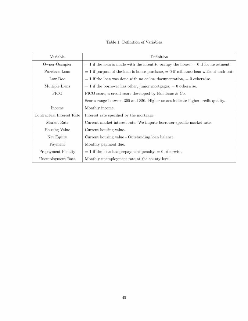
Table 1: Definition of Variables

Variable Definition

Owner-Occupier = 1 if the loan is made with the intent to occupy the house, = 0 if for investment.

Purchase Loan = 1 if purpose of the loan is house purchase, = 0 if refinance loan without cash-out.

Low Doc = 1 if the loan was done with no or low documentation, = 0 otherwise.

Multiple Liens = 1 if the borrower has other, junior mortgages, = 0 otherwise.

FICO FICO score, a credit score developed by Fair Issac & Co.

Scores range between 300 and 850. Higher scores indicate higher credit quality.

Income Monthly income.

Contractual Interest Rate Interest rate specified by the mortgage.

Market Rate Current market interest rate. We impute borrower-specific market rate.

Housing Value Current housing value.

Net Equity Current housing value - Outstanding loan balance.

Payment Monthly payment due.

Prepayment Penalty = 1 if the loan has prepayment penalty, = 0 otherwise.

Unemployment Rate Monthly unemployment rate at the county level.

45

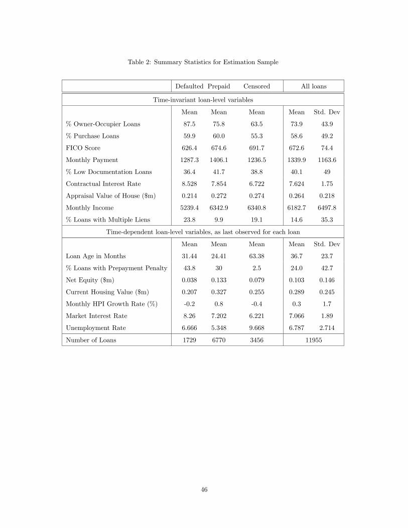
Table 2: Summary Statistics for Estimation Sample

Defaulted Prepaid Censored All loans

Time-invariant loan-level variables

Mean Mean Mean Mean Std. Dev

% Owner-Occupier Loans 87.5 75.8 63.5 73.9 43.9

% Purchase Loans 59.9 60.0 55.3 58.6 49.2

FICO Score 626.4 674.6 691.7 672.6 74.4

Monthly Payment 1287.3 1406.1 1236.5 1339.9 1163.6

% Low Documentation Loans 36.4 41.7 38.8 40.1 49

Contractual Interest Rate 8.528 7.854 6.722 7.624 1.75

Appraisal Value of House ($m) 0.214 0.272 0.274 0.264 0.218

Monthly Income 5239.4 6342.9 6340.8 6182.7 6497.8

% Loans with Multiple Liens 23.8 9.9 19.1 14.6 35.3

Time-dependent loan-level variables, as last observed for each loan

Mean Mean Mean Mean Std. Dev

Loan Age in Months 31.44 24.41 63.38 36.7 23.7

% Loans with Prepayment Penalty 43.8 30 2.5 24.0 42.7

Net Equity ($m) 0.038 0.133 0.079 0.103 0.146

Current Housing Value ($m) 0.207 0.327 0.255 0.289 0.245

Monthly HPI Growth Rate (%) -0.2 0.8 -0.4 0.3 1.7

Market Interest Rate 8.26 7.202 6.221 7.066 1.89

Unemployment Rate 6.666 5.348 9.668 6.787 2.714

Number of Loans 1729 6770 3456 11955

46

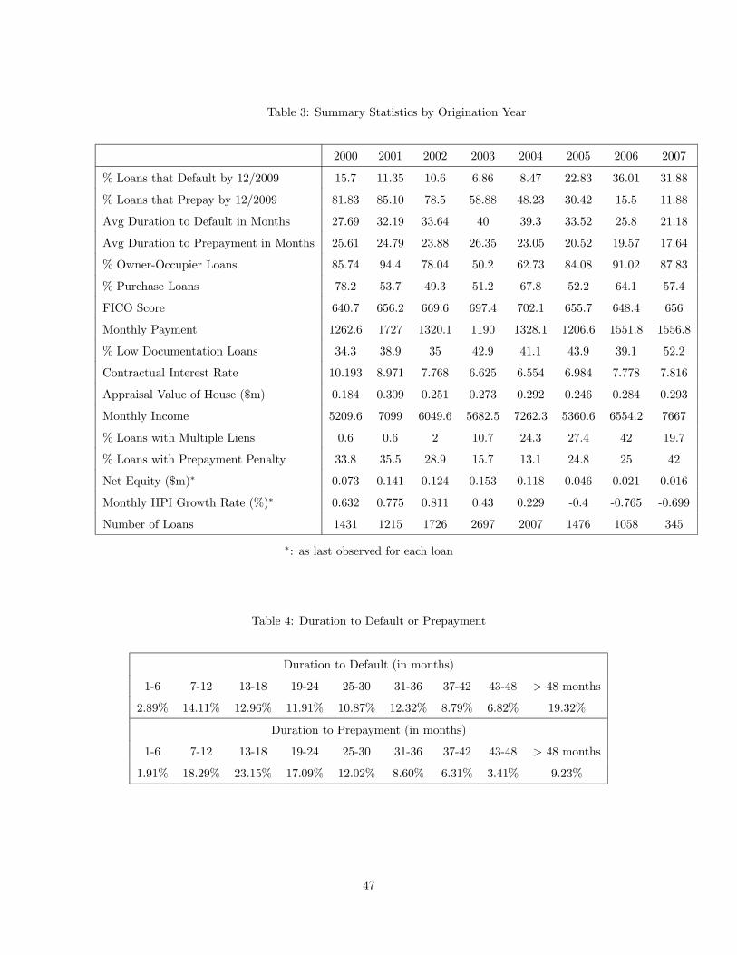
Table 3: Summary Statistics by Origination Year

2000 2001 2002 2003 2004 2005 2006 2007

% Loans that Default by 12/2009 15.7 11.35 10.6 6.86 8.47 22.83 36.01 31.88

% Loans that Prepay by 12/2009 81.83 85.10 78.5 58.88 48.23 30.42 15.5 11.88

Avg Duration to Default in Months 27.69 32.19 33.64 40 39.3 33.52 25.8 21.18

Avg Duration to Prepayment in Months 25.61 24.79 23.88 26.35 23.05 20.52 19.57 17.64

% Owner-Occupier Loans 85.74 94.4 78.04 50.2 62.73 84.08 91.02 87.83

% Purchase Loans 78.2 53.7 49.3 51.2 67.8 52.2 64.1 57.4

FICO Score 640.7 656.2 669.6 697.4 702.1 655.7 648.4 656

Monthly Payment 1262.6 1727 1320.1 1190 1328.1 1206.6 1551.8 1556.8

% Low Documentation Loans 34.3 38.9 35 42.9 41.1 43.9 39.1 52.2

Contractual Interest Rate 10.193 8.971 7.768 6.625 6.554 6.984 7.778 7.816

Appraisal Value of House ($m) 0.184 0.309 0.251 0.273 0.292 0.246 0.284 0.293

Monthly Income 5209.6 7099 6049.6 5682.5 7262.3 5360.6 6554.2 7667

% Loans with Multiple Liens 0.6 0.6 2 10.7 24.3 27.4 42 19.7

% Loans with Prepayment Penalty 33.8 35.5 28.9 15.7 13.1 24.8 25 42

Net Equity ($m)∗ 0.073 0.141 0.124 0.153 0.118 0.046 0.021 0.016

Monthly HPI Growth Rate (%)∗ 0.632 0.775 0.811 0.43 0.229 -0.4 -0.765 -0.699

Number of Loans 1431 1215 1726 2697 2007 1476 1058 345

∗: as last observed for each loan

Table 4: Duration to Default or Prepayment

Duration to Default (in months)

1-6 7-12 13-18 19-24 25-30 31-36 37-42 43-48 48 months

2.89% 14.11% 12.96% 11.91% 10.87% 12.32% 8.79% 6.82% 19.32%

Duration to Prepayment (in months)

1-6 7-12 13-18 19-24 25-30 31-36 37-42 43-48 48 months

1.91% 18.29% 23.15% 17.09% 12.02% 8.60% 6.31% 3.41% 9.23%

47

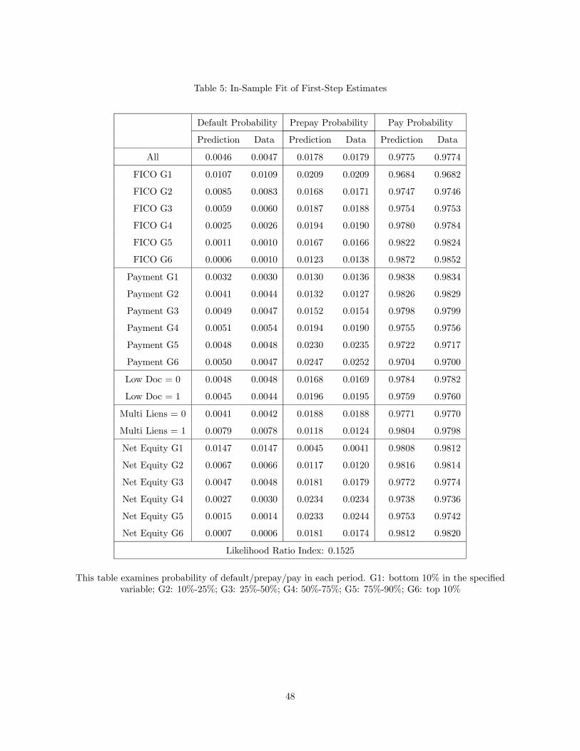
Table 5: In-Sample Fit of First-Step Estimates

Default Probability Prepay Probability Pay Probability

Prediction Data Prediction Data Prediction Data

All 0.0046 0.0047 0.0178 0.0179 0.9775 0.9774

FICO G1 0.0107 0.0109 0.0209 0.0209 0.9684 0.9682

FICO G2 0.0085 0.0083 0.0168 0.0171 0.9747 0.9746

FICO G3 0.0059 0.0060 0.0187 0.0188 0.9754 0.9753

FICO G4 0.0025 0.0026 0.0194 0.0190 0.9780 0.9784

FICO G5 0.0011 0.0010 0.0167 0.0166 0.9822 0.9824

FICO G6 0.0006 0.0010 0.0123 0.0138 0.9872 0.9852

Payment G1 0.0032 0.0030 0.0130 0.0136 0.9838 0.9834

Payment G2 0.0041 0.0044 0.0132 0.0127 0.9826 0.9829

Payment G3 0.0049 0.0047 0.0152 0.0154 0.9798 0.9799

Payment G4 0.0051 0.0054 0.0194 0.0190 0.9755 0.9756

Payment G5 0.0048 0.0048 0.0230 0.0235 0.9722 0.9717

Payment G6 0.0050 0.0047 0.0247 0.0252 0.9704 0.9700

Low Doc = 0 0.0048 0.0048 0.0168 0.0169 0.9784 0.9782

Low Doc = 1 0.0045 0.0044 0.0196 0.0195 0.9759 0.9760

Multi Liens = 0 0.0041 0.0042 0.0188 0.0188 0.9771 0.9770

Multi Liens = 1 0.0079 0.0078 0.0118 0.0124 0.9804 0.9798

Net Equity G1 0.0147 0.0147 0.0045 0.0041 0.9808 0.9812

Net Equity G2 0.0067 0.0066 0.0117 0.0120 0.9816 0.9814

Net Equity G3 0.0047 0.0048 0.0181 0.0179 0.9772 0.9774

Net Equity G4 0.0027 0.0030 0.0234 0.0234 0.9738 0.9736

Net Equity G5 0.0015 0.0014 0.0233 0.0244 0.9753 0.9742

Net Equity G6 0.0007 0.0006 0.0181 0.0174 0.9812 0.9820

Likelihood Ratio Index: 0.1525

This table examines probability of default/prepay/pay in each period. G1: bottom 10% in the specified

variable; G2: 10%-25%; G3: 25%-50%; G4: 50%-75%; G5: 75%-90%; G6: top 10%

48

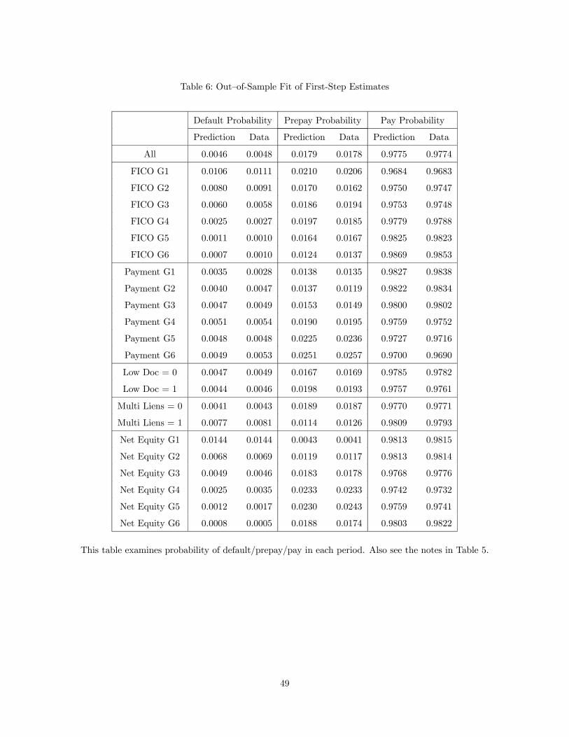
Table 6: Out—of-Sample Fit of First-Step Estimates

Default Probability Prepay Probability Pay Probability

Prediction Data Prediction Data Prediction Data

All 0.0046 0.0048 0.0179 0.0178 0.9775 0.9774

FICO G1 0.0106 0.0111 0.0210 0.0206 0.9684 0.9683

FICO G2 0.0080 0.0091 0.0170 0.0162 0.9750 0.9747

FICO G3 0.0060 0.0058 0.0186 0.0194 0.9753 0.9748

FICO G4 0.0025 0.0027 0.0197 0.0185 0.9779 0.9788

FICO G5 0.0011 0.0010 0.0164 0.0167 0.9825 0.9823

FICO G6 0.0007 0.0010 0.0124 0.0137 0.9869 0.9853

Payment G1 0.0035 0.0028 0.0138 0.0135 0.9827 0.9838

Payment G2 0.0040 0.0047 0.0137 0.0119 0.9822 0.9834

Payment G3 0.0047 0.0049 0.0153 0.0149 0.9800 0.9802

Payment G4 0.0051 0.0054 0.0190 0.0195 0.9759 0.9752

Payment G5 0.0048 0.0048 0.0225 0.0236 0.9727 0.9716

Payment G6 0.0049 0.0053 0.0251 0.0257 0.9700 0.9690

Low Doc = 0 0.0047 0.0049 0.0167 0.0169 0.9785 0.9782

Low Doc = 1 0.0044 0.0046 0.0198 0.0193 0.9757 0.9761

Multi Liens = 0 0.0041 0.0043 0.0189 0.0187 0.9770 0.9771

Multi Liens = 1 0.0077 0.0081 0.0114 0.0126 0.9809 0.9793

Net Equity G1 0.0144 0.0144 0.0043 0.0041 0.9813 0.9815

Net Equity G2 0.0068 0.0069 0.0119 0.0117 0.9813 0.9814

Net Equity G3 0.0049 0.0046 0.0183 0.0178 0.9768 0.9776

Net Equity G4 0.0025 0.0035 0.0233 0.0233 0.9742 0.9732

Net Equity G5 0.0012 0.0017 0.0230 0.0243 0.9759 0.9741

Net Equity G6 0.0008 0.0005 0.0188 0.0174 0.9803 0.9822

This table examines probability of default/prepay/pay in each period. Also see the notes in Table 5.

49

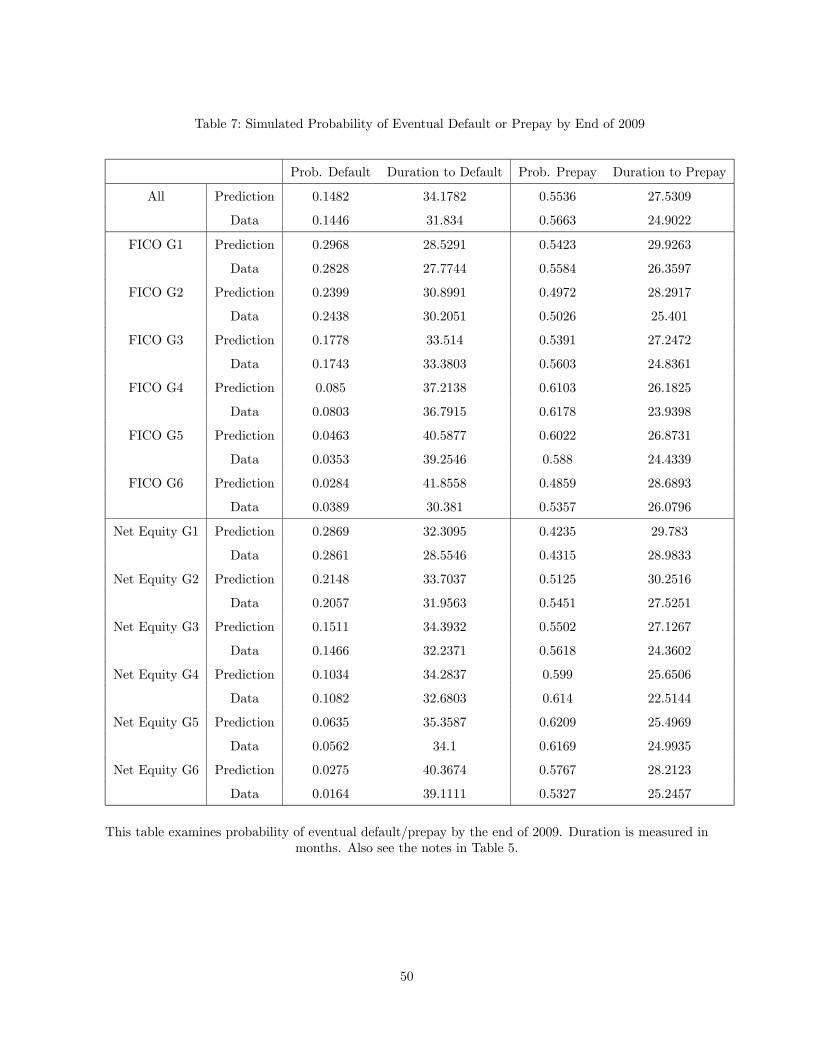
Table 7: Simulated Probability of Eventual Default or Prepay by End of 2009

Prob. Default Duration to Default Prob. Prepay Duration to Prepay

All Prediction 0.1482 34.1782 0.5536 27.5309

Data 0.1446 31.834 0.5663 24.9022

FICO G1 Prediction 0.2968 28.5291 0.5423 29.9263

Data 0.2828 27.7744 0.5584 26.3597

FICO G2 Prediction 0.2399 30.8991 0.4972 28.2917

Data 0.2438 30.2051 0.5026 25.401

FICO G3 Prediction 0.1778 33.514 0.5391 27.2472

Data 0.1743 33.3803 0.5603 24.8361

FICO G4 Prediction 0.085 37.2138 0.6103 26.1825

Data 0.0803 36.7915 0.6178 23.9398

FICO G5 Prediction 0.0463 40.5877 0.6022 26.8731

Data 0.0353 39.2546 0.588 24.4339

FICO G6 Prediction 0.0284 41.8558 0.4859 28.6893

Data 0.0389 30.381 0.5357 26.0796

Net Equity G1 Prediction 0.2869 32.3095 0.4235 29.783

Data 0.2861 28.5546 0.4315 28.9833

Net Equity G2 Prediction 0.2148 33.7037 0.5125 30.2516

Data 0.2057 31.9563 0.5451 27.5251

Net Equity G3 Prediction 0.1511 34.3932 0.5502 27.1267

Data 0.1466 32.2371 0.5618 24.3602

Net Equity G4 Prediction 0.1034 34.2837 0.599 25.6506

Data 0.1082 32.6803 0.614 22.5144

Net Equity G5 Prediction 0.0635 35.3587 0.6209 25.4969

Data 0.0562 34.1 0.6169 24.9935

Net Equity G6 Prediction 0.0275 40.3674 0.5767 28.2123

Data 0.0164 39.1111 0.5327 25.2457

This table examines probability of eventual default/prepay by the end of 2009. Duration is measured in

months. Also see the notes in Table 5.

50

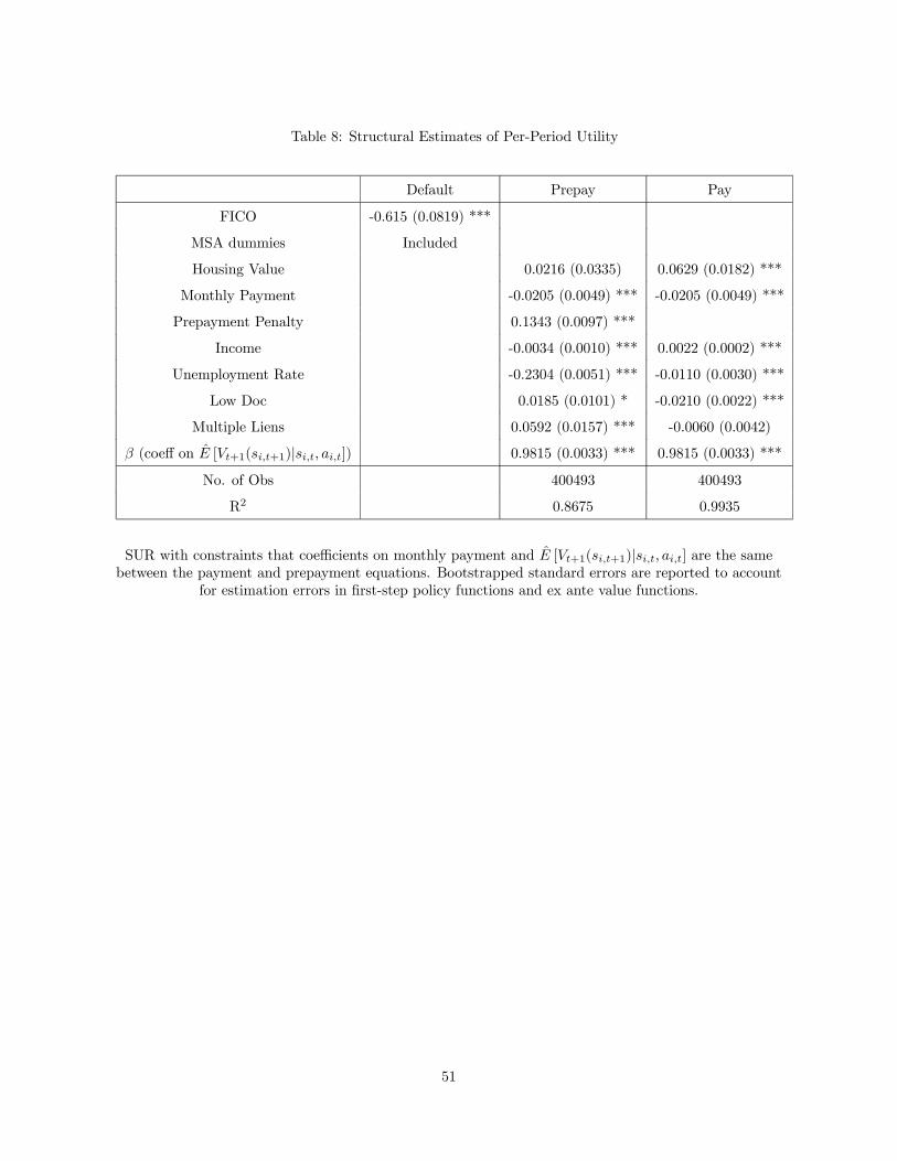
Table 8: Structural Estimates of Per-Period Utility

Default Prepay Pay

FICO -0.615 (0.0819) ***

MSA dummies Included

Housing Value 0.0216 (0.0335) 0.0629 (0.0182) ***

Monthly Payment -0.0205 (0.0049) *** -0.0205 (0.0049) ***

Prepayment Penalty 0.1343 (0.0097) ***

Income -0.0034 (0.0010) *** 0.0022 (0.0002) ***

Unemployment Rate -0.2304 (0.0051) *** -0.0110 (0.0030) ***

Low Doc 0.0185 (0.0101) * -0.0210 (0.0022) ***

Multiple Liens 0.0592 (0.0157) *** -0.0060 (0.0042)

(coeff on [+1(+1)| ]) 0.9815 (0.0033) *** 0.9815 (0.0033) ***

No. of Obs 400493 400493

R2 0.8675 0.9935

SUR with constraints that coefficients on monthly payment and [+1(+1)| ] are the samebetween the payment and prepayment equations. Bootstrapped standard errors are reported to account

for estimation errors in first-step policy functions and ex ante value functions.

51

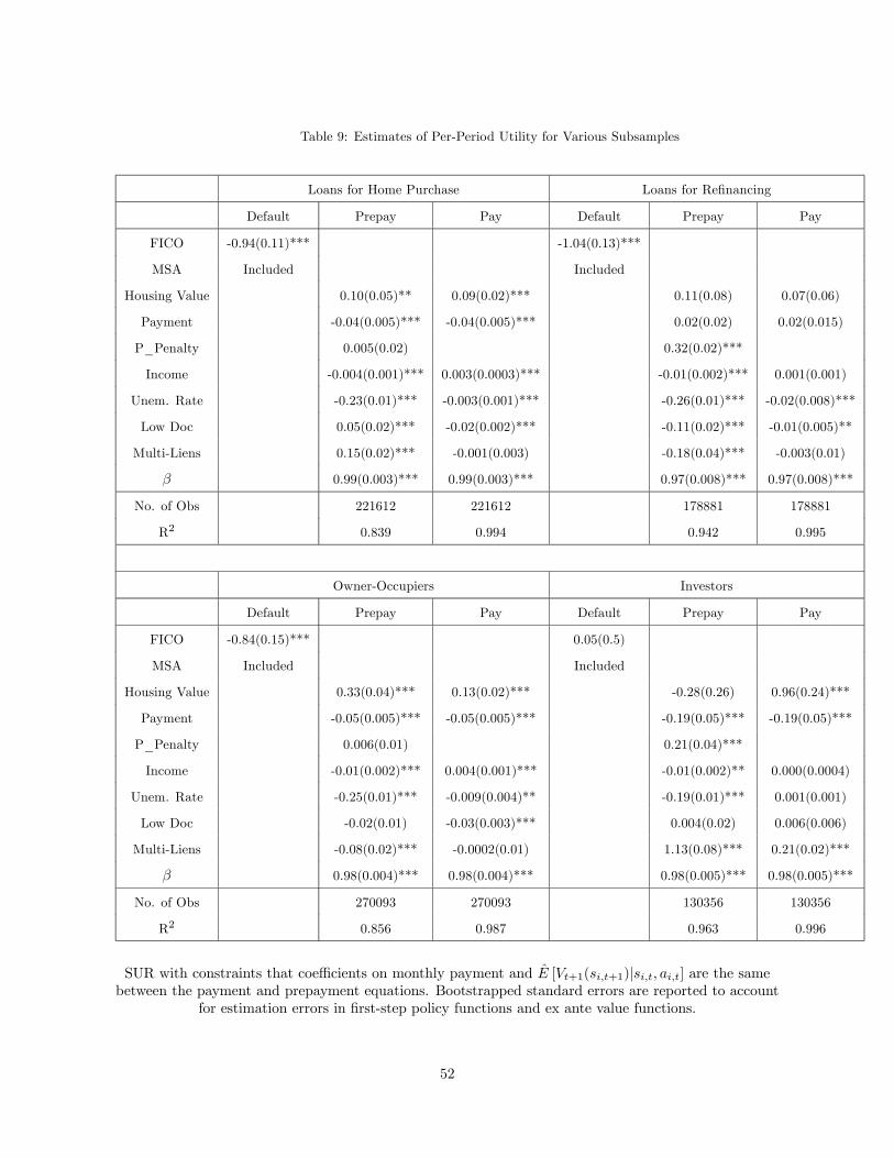
Table 9: Estimates of Per-Period Utility for Various Subsamples

Loans for Home Purchase Loans for Refinancing

Default Prepay Pay Default Prepay Pay

FICO -0.94(0.11)*** -1.04(0.13)***

MSA Included Included

Housing Value 0.10(0.05)** 0.09(0.02)*** 0.11(0.08) 0.07(0.06)

Payment -0.04(0.005)*** -0.04(0.005)*** 0.02(0.02) 0.02(0.015)

P_Penalty 0.005(0.02) 0.32(0.02)***

Income -0.004(0.001)*** 0.003(0.0003)*** -0.01(0.002)*** 0.001(0.001)

Unem. Rate -0.23(0.01)*** -0.003(0.001)*** -0.26(0.01)*** -0.02(0.008)***

Low Doc 0.05(0.02)*** -0.02(0.002)*** -0.11(0.02)*** -0.01(0.005)**

Multi-Liens 0.15(0.02)*** -0.001(0.003) -0.18(0.04)*** -0.003(0.01)

0.99(0.003)*** 0.99(0.003)*** 0.97(0.008)*** 0.97(0.008)***

No. of Obs 221612 221612 178881 178881

R2 0.839 0.994 0.942 0.995

Owner-Occupiers Investors

Default Prepay Pay Default Prepay Pay

FICO -0.84(0.15)*** 0.05(0.5)

MSA Included Included

Housing Value 0.33(0.04)*** 0.13(0.02)*** -0.28(0.26) 0.96(0.24)***

Payment -0.05(0.005)*** -0.05(0.005)*** -0.19(0.05)*** -0.19(0.05)***

P_Penalty 0.006(0.01) 0.21(0.04)***

Income -0.01(0.002)*** 0.004(0.001)*** -0.01(0.002)** 0.000(0.0004)

Unem. Rate -0.25(0.01)*** -0.009(0.004)** -0.19(0.01)*** 0.001(0.001)

Low Doc -0.02(0.01) -0.03(0.003)*** 0.004(0.02) 0.006(0.006)

Multi-Liens -0.08(0.02)*** -0.0002(0.01) 1.13(0.08)*** 0.21(0.02)***

0.98(0.004)*** 0.98(0.004)*** 0.98(0.005)*** 0.98(0.005)***

No. of Obs 270093 270093 130356 130356

R2 0.856 0.987 0.963 0.996

SUR with constraints that coefficients on monthly payment and [+1(+1)| ] are the samebetween the payment and prepayment equations. Bootstrapped standard errors are reported to account

for estimation errors in first-step policy functions and ex ante value functions.

52

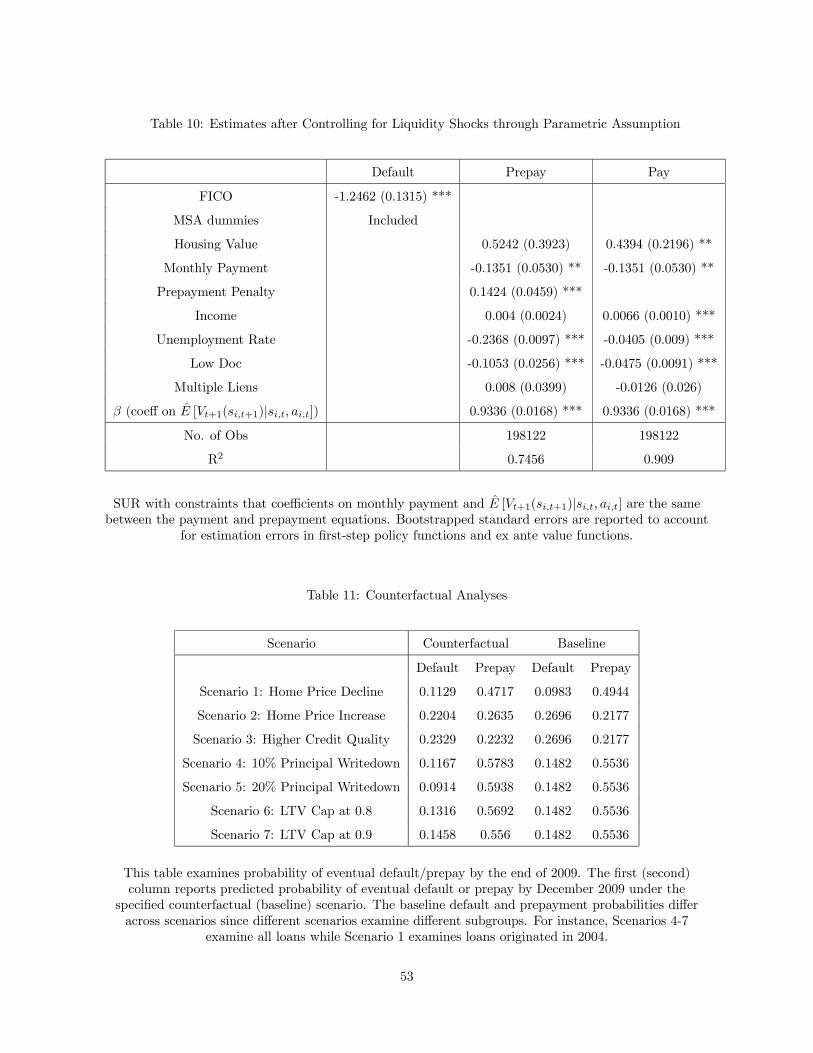
Table 10: Estimates after Controlling for Liquidity Shocks through Parametric Assumption

Default Prepay Pay

FICO -1.2462 (0.1315) ***

MSA dummies Included

Housing Value 0.5242 (0.3923) 0.4394 (0.2196) **

Monthly Payment -0.1351 (0.0530) ** -0.1351 (0.0530) **

Prepayment Penalty 0.1424 (0.0459) ***

Income 0.004 (0.0024) 0.0066 (0.0010) ***

Unemployment Rate -0.2368 (0.0097) *** -0.0405 (0.009) ***

Low Doc -0.1053 (0.0256) *** -0.0475 (0.0091) ***

Multiple Liens 0.008 (0.0399) -0.0126 (0.026)

(coeff on [+1(+1)| ]) 0.9336 (0.0168) *** 0.9336 (0.0168) ***

No. of Obs 198122 198122

R2 0.7456 0.909

SUR with constraints that coefficients on monthly payment and [+1(+1)| ] are the samebetween the payment and prepayment equations. Bootstrapped standard errors are reported to account

for estimation errors in first-step policy functions and ex ante value functions.

Table 11: Counterfactual Analyses

Scenario Counterfactual Baseline

Default Prepay Default Prepay

Scenario 1: Home Price Decline 0.1129 0.4717 0.0983 0.4944

Scenario 2: Home Price Increase 0.2204 0.2635 0.2696 0.2177

Scenario 3: Higher Credit Quality 0.2329 0.2232 0.2696 0.2177

Scenario 4: 10% Principal Writedown 0.1167 0.5783 0.1482 0.5536

Scenario 5: 20% Principal Writedown 0.0914 0.5938 0.1482 0.5536

Scenario 6: LTV Cap at 0.8 0.1316 0.5692 0.1482 0.5536

Scenario 7: LTV Cap at 0.9 0.1458 0.556 0.1482 0.5536

This table examines probability of eventual default/prepay by the end of 2009. The first (second)

column reports predicted probability of eventual default or prepay by December 2009 under the

specified counterfactual (baseline) scenario. The baseline default and prepayment probabilities differ

across scenarios since different scenarios examine different subgroups. For instance, Scenarios 4-7

examine all loans while Scenario 1 examines loans originated in 2004.

53

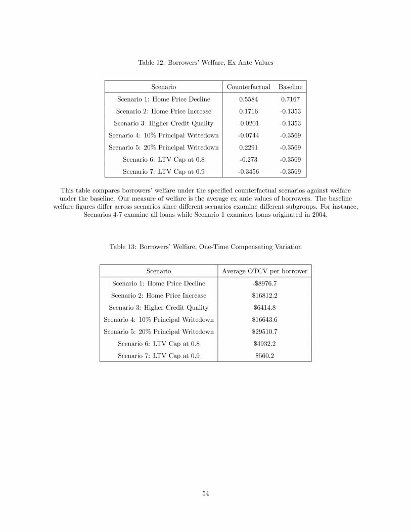
Table 12: Borrowers’ Welfare, Ex Ante Values

Scenario Counterfactual Baseline

Scenario 1: Home Price Decline 0.5584 0.7167

Scenario 2: Home Price Increase 0.1716 -0.1353

Scenario 3: Higher Credit Quality -0.0201 -0.1353

Scenario 4: 10% Principal Writedown -0.0744 -0.3569

Scenario 5: 20% Principal Writedown 0.2291 -0.3569

Scenario 6: LTV Cap at 0.8 -0.273 -0.3569

Scenario 7: LTV Cap at 0.9 -0.3456 -0.3569

This table compares borrowers’ welfare under the specified counterfactual scenarios against welfare

under the baseline. Our measure of welfare is the average ex ante values of borrowers. The baseline

welfare figures differ across scenarios since different scenarios examine different subgroups. For instance,

Scenarios 4-7 examine all loans while Scenario 1 examines loans originated in 2004.

Table 13: Borrowers’ Welfare, One-Time Compensating Variation

Scenario Average OTCV per borrower

Scenario 1: Home Price Decline -$8976.7

Scenario 2: Home Price Increase $16812.2

Scenario 3: Higher Credit Quality $6414.8

Scenario 4: 10% Principal Writedown $16643.6

Scenario 5: 20% Principal Writedown $29510.7

Scenario 6: LTV Cap at 0.8 $4932.2

Scenario 7: LTV Cap at 0.9 $560.2

54

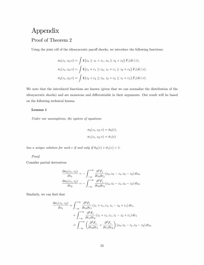
Appendix

Proof of Theorem 2

Using the joint cdf of the idiosyncratic payoff shocks, we introduce the following functions:

0(1 2; ) =

Z10 ≥ 1 + 1 0 ≥ 2 + 2( | )

1(1 2; ) =

Z11 + 1 ≥ 0 1 + 1 ≥ 2 + 2( | )

2(1 2; ) =

Z12 + 2 ≥ 0 2 + 2 ≥ 1 + 1( | )

We note that the introduced functions are known (given that we can normalize the distribution of the

idiosyncratic shocks) and are monotone and differentiable in their arguments. Our result will be based

on the following technical lemma.

Lemma 1

Under our assumptions, the system of equations

0(1 2; ) = 0()

1(1 2; ) = 1()

has a unique solution for each if and only if 0(c) + 1(c) 1.

Proof:

Consider partial derivatives

0(1 2)

1= −

Z +∞

−∞

2

01(0 0 − 1 0 − 2) 0

0(1 2)

2= −

Z +∞

−∞

2

02(0 0 − 1 0 − 2) 0

Similarly, we can find that

1(1 2)

1=

Z +∞

−∞

2

01(1 + 1 1 1 − 2 + 1) 1

+

Z +∞

−∞

2

12(1 + 1 1 1 − 2 + 1) 1

=

Z +∞

−∞

µ2

01+

2

12

¶(0 0 − 1 0 − 2) 0

55

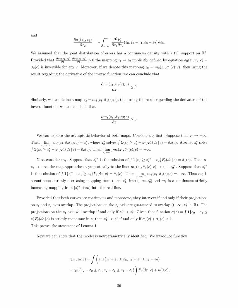
and1(1 2)

2= −

Z +∞

−∞

2

12(0 0 − 1 0 − 2) 0

We assumed that the joint distribution of errors has a continuous density with a full support on R3.

Provided that0(12)

1

0(12)

2 0 the mapping 1 7→ 2 implicitly defined by equation 0(1 2; ) =

0() is invertible for any . Moreover, if we denote this mapping 2 = 0(1 0(); ), then using the

result regarding the derivative of the inverse function, we can conclude that

0(1 0(); )

1≤ 0

Similarly, we can define a map 2 = 1(1 1(); ), then using the result regarding the derivative of the

inverse function, we can conclude that

1(1 1(); )

1≥ 0

We can explore the asymptotic behavior of both maps. Consider 0 first. Suppose that 1 → −∞.Then lim

1→−∞0(1 0(); ) = ∗2 , where

∗2 solves

R10 ≥ ∗2 + 2( | ) = 0(). Also let

∗1 solveR

10 ≥ ∗1 + 1( | ) = 0(). Then lim1→∗1

0(1 0(); ) = −∞.

Next consider 1. Suppose that ∗∗2 is the solution of

R11 ≥ ∗∗2 + 2( | ) = 1(). Then as

1 → +∞, the map approaches asymptotically to the line: 1(1 1(); )→ 1 + ∗∗2 . Suppose that ∗∗1

is the solution ofR1∗∗1 + 1 ≥ 0( | ) = 1(). Then lim

1→∗∗11(1 1(); ) = −∞. Thus 0 is

a continuous strictly decreasing mapping from (−∞ ∗1 ] into (−∞ ∗2 ] and 1 is a continuous strictly

increasing mapping from [∗∗1 +∞) into the real line.

Provided that both curves are continuous and monotone, they intersect if and only if their projections

on 1 and 2 axes overlap. The projections on the 2 axis are guaranteed to overlap ((−∞ ∗2 ] ⊂ R). Theprojections on the 1 axis will overlap if and only if

∗∗1 ∗1 . Given that function () =

R10 − 1 ≤

( | ) is strictly monotone in , then ∗∗1 ∗1 if and only if 0() + 1() 1.

This proves the statement of Lemma 1.

Next we can show that the model is nonparametrically identified. We introduce function

(1 2; ) =

Z µ111 + 1 ≥ 0 1 + 1 ≥ 2 + 2

+ 212 + 2 ≥ 0 2 + 2 ≥ 1 + 1¶( | ) + (0; )

56

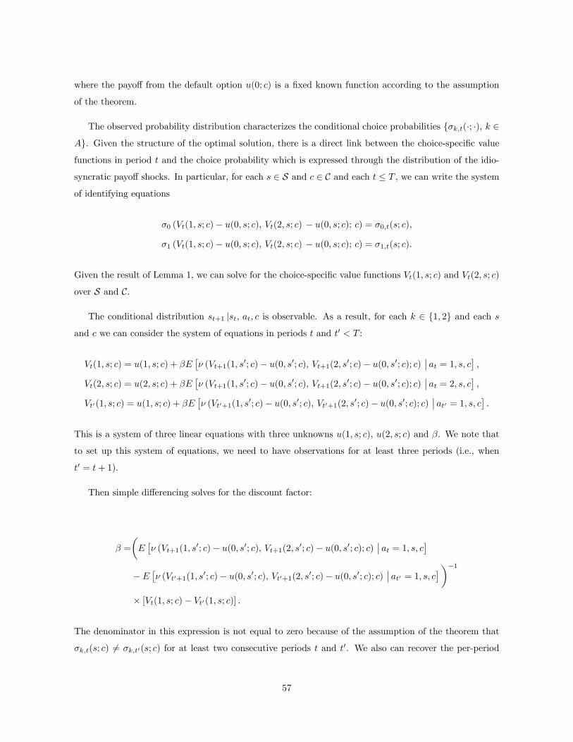
where the payoff from the default option (0; ) is a fixed known function according to the assumption

of the theorem.

The observed probability distribution characterizes the conditional choice probabilities (·; ·) ∈. Given the structure of the optimal solution, there is a direct link between the choice-specific valuefunctions in period and the choice probability which is expressed through the distribution of the idio-

syncratic payoff shocks. In particular, for each ∈ S and ∈ C and each ≤ , we can write the system

of identifying equations

0 ((1 ; )− (0 ; ) (2 ; ) − (0 ; ); ) = 0(; )

1 ((1 ; )− (0 ; ) (2 ; ) − (0 ; ); ) = 1(; )

Given the result of Lemma 1, we can solve for the choice-specific value functions (1 ; ) and (2 ; )

over S and C.

The conditional distribution +1 | is observable. As a result, for each ∈ 1 2 and each

and we can consider the system of equations in periods and 0 :

(1 ; ) = (1 ; ) + £ (+1(1

0; )− (0 0; ) +1(2 0; )− (0 0; ); )¯ = 1

¤

(2 ; ) = (2 ; ) + £ (+1(1

0; )− (0 0; ) +1(2 0; )− (0 0; ); )¯ = 2

¤

0(1 ; ) = (1 ; ) + £ (0+1(1

0; )− (0 0; ) 0+1(2 0; )− (0 0; ); )¯0 = 1

¤

This is a system of three linear equations with three unknowns (1 ; ), (2 ; ) and . We note that

to set up this system of equations, we need to have observations for at least three periods (i.e., when

0 = + 1).

Then simple differencing solves for the discount factor:

=

µ£ (+1(1

0; )− (0 0; ) +1(2 0; )− (0 0; ); )¯ = 1

¤−

£ (0+1(1

0; )− (0 0; ) 0+1(2 0; )− (0 0; ); )¯0 = 1

¤¶−1× [(1 ; )− 0(1 ; )]

The denominator in this expression is not equal to zero because of the assumption of the theorem that

(; ) 6= 0(; ) for at least two consecutive periods and 0. We also can recover the per-period

57

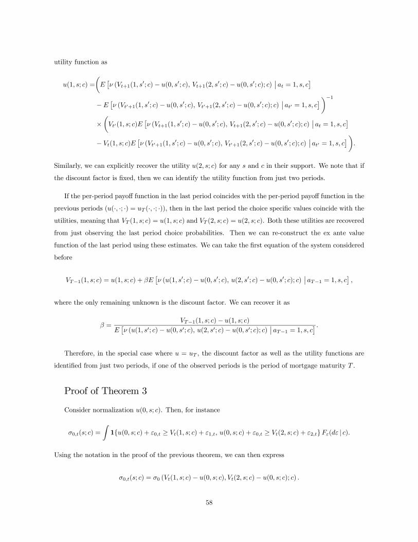
utility function as

(1 ; ) =

µ£ (+1(1

0; )− (0 0; ) +1(2 0; )− (0 0; ); )¯ = 1

¤−

£ (0+1(1

0; )− (0 0; ) 0+1(2 0; )− (0 0; ); )¯0 = 1

¤¶−1×µ0(1 ; )

£ (+1(1

0; )− (0 0; ) +1(2 0; )− (0 0; ); )¯ = 1

¤− (1 ; )

£ (0+1(1

0; )− (0 0; ) 0+1(2 0; )− (0 0; ); )¯0 = 1

¤¶

Similarly, we can explicitly recover the utility (2 ; ) for any and in their support. We note that if

the discount factor is fixed, then we can identify the utility function from just two periods.

If the per-period payoff function in the last period coincides with the per-period payoff function in the

previous periods ((· ·; ·) = (· ·; ·)), then in the last period the choice specific values coincide with theutilities, meaning that (1 ; ) = (1 ; ) and (2 ; ) = (2 ; ). Both these utilities are recovered

from just observing the last period choice probabilities. Then we can re-construct the ex ante value

function of the last period using these estimates. We can take the first equation of the system considered

before

−1(1 ; ) = (1 ; ) + £ ((1 0; )− (0 0; ) (2 0; )− (0 0; ); )

¯−1 = 1

¤

where the only remaining unknown is the discount factor. We can recover it as

=−1(1 ; )− (1 ; )

£ ((1 0; )− (0 0; ) (2 0; )− (0 0; ); )

¯−1 = 1

¤ Therefore, in the special case where = , the discount factor as well as the utility functions are

identified from just two periods, if one of the observed periods is the period of mortgage maturity .

Proof of Theorem 3

Consider normalization (0 ; ). Then, for instance

0(; ) =

Z1(0 ; ) + 0 ≥ (1 ; ) + 1 (0 ; ) + 0 ≥ (2 ; ) + 2( | )

Using the notation in the proof of the previous theorem, we can then express

0(; ) = 0 ((1 ; )− (0 ; ) (2 ; )− (0 ; ); )

58

We can also provide similar expressions for other choices. Then we solve the system of equations

0(; ) = 0 ((1 ; )− (0 ; ) (2 ; )− (0 ; ); )

1(; ) = 1 ((1 ; )− (0 ; ) (2 ; )− (0 ; ); )

to recover the value functions. We note that the recovered differences ( ; )− (0 ; ) are invariant

to the choice of (0 ; ) as they are directly recovered from the data.

The ex ante value function can be recovered as

(; ) =

Z µ((1 ; )− (0 ; ))1(1 ; )− (0 ; ) + 1 ≥ 0 (1 ; ) + 1

≥ (2 ; ) + 2+ ((2 ; )− (0 ; ))1(2 ; )− (0 ; ) + 2 ≥ 0 (2 ; ) + 2

≥ (1 ; ) + 1¶( | )

+ (0 ; ) = V(; ) + (0 ; )

where function V(·; ·) is invariant to the choice of the default payoff (it is determined by the observedchoice probabilities). The system of equations identifying the per-period payoffs takes the form

(1 ; ) = (1 ; ) + £V+1(

0; ) + (0 0; )¯ = 1

¤

(2 ; ) = (2 ; ) + £V+1(

0; ) + (0 0; )¯ = 2

¤

0(1 ; ) = (1 ; ) + £V0+1(

0; ) + (0 0; )¯0 = 1

¤

Provided that (0 ; ) is normalized to a fixed function, taking the difference between the first and the

third equation allows us to express the discount factor as

=(1 ; )− (0 ; )− (0(1 ; )− (0 ; ))

£V+1(0; )

¯ = 1

¤−£V0+1(0; )

¯0 = 1

¤ Provided that the numerator and the denominator are invariant with respect to the choice of the default

utility (as they can be directly recovered from the observed choice probabilities), the discount factor will

not depend on that choice either. Having obtained the discount factor, we can focus on the first two

59

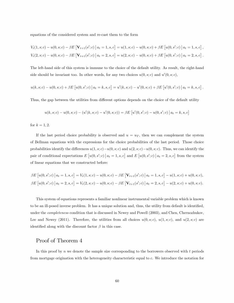
equations of the considered system and re-cast them to the form

(1 ; )− (0 ; )− £V+1(

0; )¯ = 1

¤= (1 ; )− (0 ; ) +

£(0 0; )

¯ = 1

¤

(2 ; )− (0 ; )− £V+1(

0; )¯ = 2

¤= (2 ; )− (0 ; ) +

£(0 0; )

¯ = 2

¤

The left-hand side of this system is immune to the choice of the default utility. As result, the right-hand

side should be invariant too. In other words, for any two choices (0 ; ) and 0(0 ; ),

( ; )− (0 ; ) + £(0 0; )

¯ =

¤= 0( ; )− 0(0 ; ) +

£0(0 0; )

¯ =

¤

Thus, the gap between the utilities from different options depends on the choice of the default utility

( ; )− (0 ; )− (0( ; )− 0(0 ; )) = £0(0 0; )− (0 0; )

¯ =

¤for = 1 2.

If the last period choice probability is observed and = , then we can complement the system

of Bellman equations with the expressions for the choice probabilities of the last period. Those choice

probabilities identify the differences (1 ; )−(0 ; ) and (2 ; )−(0 ; ). Thus, we can identify thepair of conditional expectations

£(0 0; )

¯ = 1

¤and

£(0 0; )

¯ = 2

¤from the system

of linear equations that we constructed before:

£(0 0; )

¯ = 1

¤= (1 ; )− (0 ; )−

£V+1(

0; )¯ = 1

¤− (1 ; ) + (0 ; )

£(0 0; )

¯ = 2

¤= (2 ; )− (0 ; )−

£V+1(

0; )¯ = 2

¤− (2 ; ) + (0 ; )

This system of equations represents a familiar nonlinear instrumental variable problem which is known

to be an ill-posed inverse problem. It has a unique solution and, thus, the utility from default is identified,

under the completeness condition that is discussed in Newey and Powell (2003), and Chen, Chernozhukov,

Lee and Newey (2011). Therefore, the utilities from all choices (0 ; ), (1 ; ), and (2 ; ) are

identified along with the discount factor in this case.

Proof of Theorem 4

In this proof by we denote the sample size corresponding to the borrowers observed with periods

from mortgage origination with the heterogeneity characteristic equal to . We introduce the notation for

60

the trinomial logit function (1 2) =exp(1)

1+exp(1)+exp(2). By (; ) we denote the choice probability

(; ) = (0( )() 0( )()) 6=

where ( ) are the coefficients of the projection of the probability ratio log(;)

0(;)on first

orthogonal polynomials. We also denote 0(; ) = 1− 1(; )− 2(; ). We note that1

2≤ 1

2

Thus, 12is a uniform Lipschitz constant and

sup∈S

|(; )− (; )| = sup∈S

¯¯Ãlog

(; )

0(; ) log

(; )

0(; )

!−

µlog

(; )

0(; ) log

(; )

0(; )

¶¯¯

≤ 12

vuutsup∈S

¯¯log 1(; )0(; )

− log 1(; )0(; )

¯¯2

+ sup∈S

¯¯log 2(; )0(; )

− log 2(; )0(; )

¯¯2

= (−)

This guarantees the quality of approximation of the choice probability using a logit transformation of the

series expansion.

Now we omit index in the variables (whenever the period of time under consideration is known) and

construct function

( ; 1

2 ) = (1 = 1− 1 = 0)

¡01 ()

02 ()

¢+ (1 = 2− 1 = 0)

¡02 ()

01 ()

¢

Then we can express the sample quasi-likelihood as

b(1 2 ) =

£( ;

1

2 )¤+ [1 = 0]

where we adopted the notation from the empirical process theory where [·] = 1

P=1. Also introduce

the population likelihood with the series expansion

(1 2 ) =

£( ;

1

2 )¤+ [1 = 0]

Consider function

( ; 1

2

1

2 ) = ( ;

1

2 )− ( ;

1

2 )−[( ;

1

2 )] +[( ;

1

2 )]

61

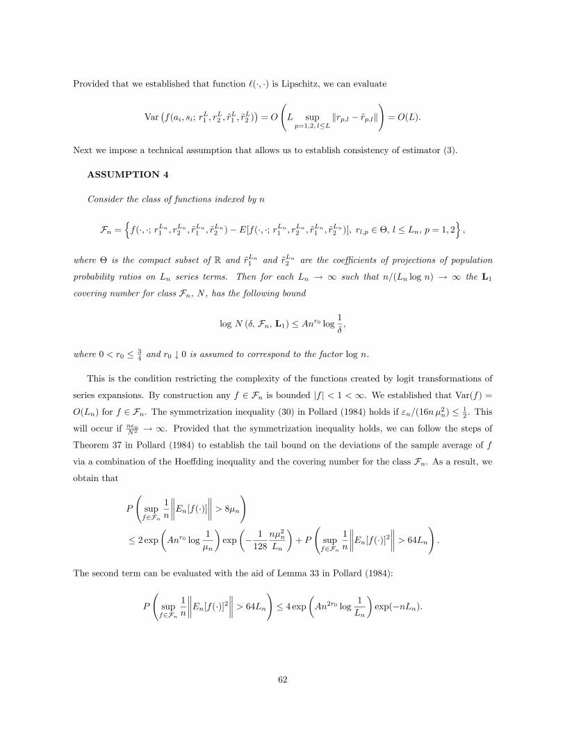
Provided that we established that function (· ·) is Lipschitz, we can evaluate

Var¡( ;

1

2

1

2 )¢=

à sup=12 ≤

k − k!= ()

Next we impose a technical assumption that allows us to establish consistency of estimator (3).

ASSUMPTION 4

Consider the class of functions indexed by

F =n(· ·; 1 2 1 2 )−[(· ·; 1 2 1 2 )] ∈ Θ ≤ = 1 2

o

where Θ is the compact subset of R and 1 and 2 are the coefficients of projections of population

probability ratios on series terms. Then for each → ∞ such that ( log ) → ∞ the L1

covering number for class F, N , has the following bound

log ( F L1) ≤ 0 log1

where 0 0 ≤ 34and 0 ↓ 0 is assumed to correspond to the factor log .

This is the condition restricting the complexity of the functions created by logit transformations of

series expansions. By construction any ∈ F is bounded | | 1 ∞. We established that Var() =() for ∈ F. The symmetrization inequality (30) in Pollard (1984) holds if (162) ≤ 1

2. This

will occur if 2 → ∞. Provided that the symmetrization inequality holds, we can follow the steps of

Theorem 37 in Pollard (1984) to establish the tail bound on the deviations of the sample average of

via a combination of the Hoeffding inequality and the covering number for the class F. As a result, weobtain that

Ãsup∈F

1

°°°°[(·)]°°°° 8

!

≤ 2 expµ0 log

1

¶exp

µ− 1

128

2

¶+

Ãsup∈F

1

°°°°[(·)]2°°°° 64

!

The second term can be evaluated with the aid of Lemma 33 in Pollard (1984):

Ãsup∈F

1

°°°°[(·)]2°°°° 64

!≤ 4 exp

µ20 log

1

¶exp(−)

62

As a result, we find that

Ãsup∈F

1

°°°°[(·)]°°°° 8

!

≤ 2 expµ0 log

1

¶exp

µ− 1

128

2

¶+ 4 exp

µ0 log

1

−

¶

We start the analysis with the first term. Consider the case with 0 0. Then the log of the first term

takes the form

0 log(1)− 1

128

2

Then one needs that2

0 log

→ ∞ if 0 0 and2

log2 → ∞ if 0 ↓ 0. Hence the first term is of

(1). This condition also guarantees that the second term vanishes. We note also that the CLT applies

to the term [1 = 0] = [1 = 0] +(1√). Now for some slowly diverging sequence →∞

such that =

q

0 log

→ 0, we establish that

sup(1

2 )∈Θ×Θ

°°° b(1 2 )−(1 2 ) +

b(1 2 )−(1 2 )°°° =

µ +

1√

¶= (1)

Thus, the sample quasi-likelihood converges uniformly to the population quasi-likelihood and the esti-

mated choice probabilities are uniformly consistent over S. To establish the rate for the estimated choiceprobabilities, we consider a neighborhood of the population projections defined by sup

=12 ≤k−k ≤

. Using Lemma 2.3.1 from van der Vaart and Wellner (1996), we can find that

"sup∈F

√[(·)]

#≤ 02

p log

1√

for some constant . Using Theorem 3.4.1 from van der Vaart and Wellner (1996) and the derived

inequality, we can express the convergence rate for the estimated parameters of the approximated choice

probabilities as 202√

1log √

≤ √. Then

sup∈S

kb(; )− (; )k =

µ

¶

To attain the rate (−14) we need to assure that

= (−14). To assure the −14 we choose

→ 0 and set = −14. Then the rate constraint can be re-written as

2−38+02

log14√√

14√√

≤ √

63

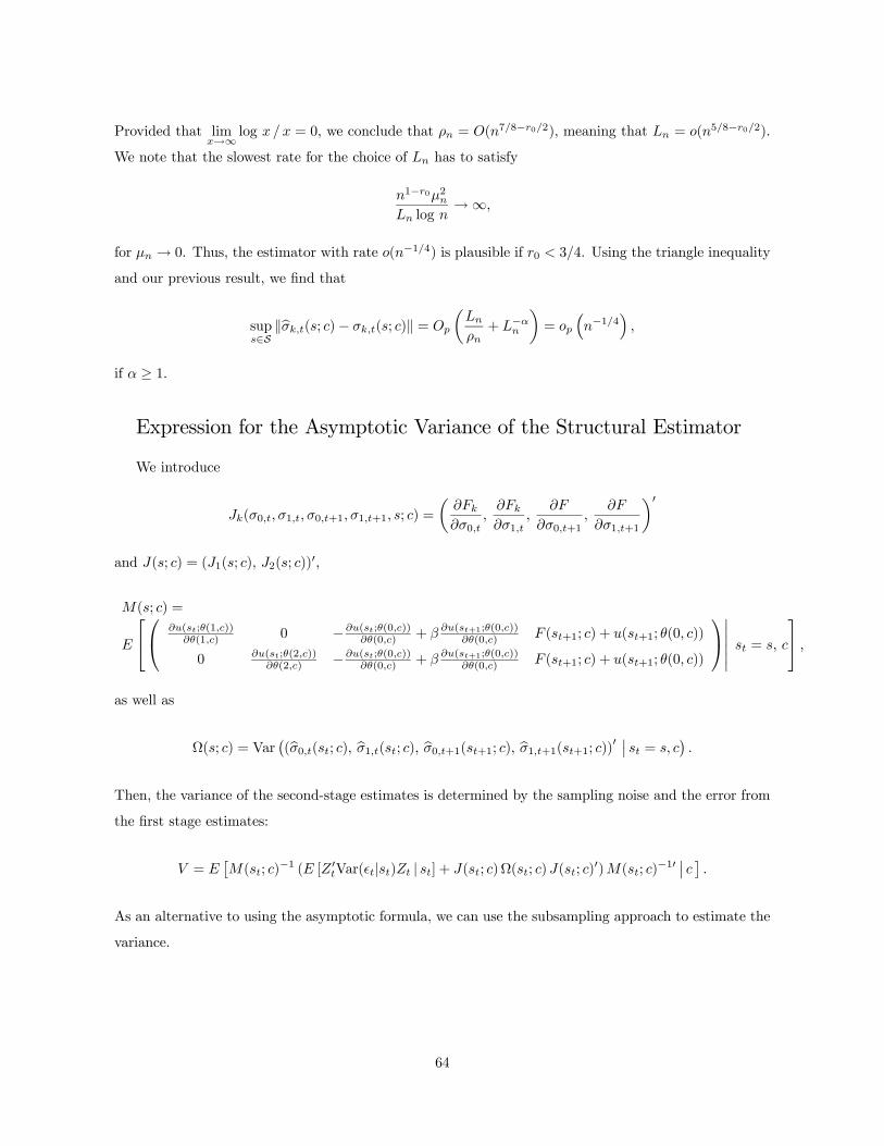
Provided that lim→∞

log = 0, we conclude that = (78−02), meaning that = (58−02).

We note that the slowest rate for the choice of has to satisfy

1−02 log

→∞

for → 0. Thus, the estimator with rate (−14) is plausible if 0 34. Using the triangle inequality

and our previous result, we find that

sup∈S

kb(; )− (; )k =

µ

+ −

¶=

³−14

´

if ≥ 1.

Expression for the Asymptotic Variance of the Structural Estimator

We introduce

(0 1 0+1 1+1 ; ) =

µ

0

1

0+1

1+1

¶0and (; ) = (1(; ) 2(; ))

0,

(; ) =

⎡⎣⎛⎝ (;(1))

(1)0 −(;(0))

(0)+

(+1;(0))

(0) (+1; ) + (+1; (0 ))

0(;(2))

(2)−(;(0))

(0)+

(+1;(0))

(0) (+1; ) + (+1; (0 ))

⎞⎠¯¯ =

⎤⎦ as well as

Ω(; ) = Var¡(b0(; ) b1(; ) b0+1(+1; ) b1+1(+1; ))0 ¯ =

¢

Then, the variance of the second-stage estimates is determined by the sampling noise and the error from

the first stage estimates:

= £(; )

−1 ( [0Var(|) | ] + (; )Ω(; )(; )0)(; )−10

¯¤

As an alternative to using the asymptotic formula, we can use the subsampling approach to estimate the

variance.

64