A Dynamic Programming Approach forValuing Corporate Debt and the TermStructure of Default Probabilities

Mohamed Ayadi, Brock University

Hatem Ben-Ameur, HEC Montréal and GERAD

Tarek Fakhfakh, FSEG Sfax

Abstract

We design and implement a dynamic program for valuing corporate-debt portfolios, seen as derivatives on a �rm�s assets, and computingits term structure of default probabilities. Our setting accommodates1- arbitrary corporate debt, 2- multiple seniority classes, 3- sinkingfunds, 4- American-style embedded options, 5- dividends, 6- tax ben-e�ts, 7- bankruptcy costs, and 8- alternative Markov dynamics forthe state process. This �exibility come at the expense of a minorloss of e¢ ciency; the analytical approach proposed in the literature isexchanged here for a numerical approach based on dynamic program-ming coupled with �nite elements. We provide several theoreticalproperties of the debt and equity value functions. Finally, we carryout a numerical study along with a sensitivity analysis, and perform anempirical investigation for selected North American public companiesto assess our construction.

Key words: Option theory, No-arbitrage pricing, Structural mod-els, Corporate-bond portfolios, Corporate bankruptcy prediction, Dy-namic programming, Finite elements, Numerical integration

1

1 Introduction

The aim of this paper is the design and implementation of a dynamic pro-gramming framework for valuing arbitrary corporate-bond portfolios, andcomputing the term structure of default probabilities. This program, basedon the structural model, is �exible and e¢ cient. Beyond the academic exer-cise, we hopefully submit a realistic setting for analyzing corporate credit risk.A corporate bankruptcy generates a loss of value for the �rm�s claimholdersand a loss of positions for the �rm�s workers. Corporate credit-risk modelsare thus useful for market participants in that they help precluding �nancialdistress and its adverse events.The option-based approach for pricing corporate bonds goes back to Mer-

ton (1974). He considers a model for a �rm with a simple capital structure,that is, a pure bond and a common stock. Then, the author builds on thefact that the stock can be seen as a European call option on the �rm�s assetswhose value moves according to a geometric Brownian motion (GBM), asset by Black and Scholes (1973). The option�s expiry date and strike priceare the bond�s maturity date and principal amount, respectively. As well,holding the pure bond is equivalent to holding the entire �rm and selling aEuropean call option to equityholders to buy the �rm at the bond�s maturityfor its principal amount.This pioneering paper has given rise to an extensive literature, known as

the structural model, where the value of a �rm�s debt and equity are expressedas functions of time and the value of the �rm�s assets (the state variable).As well, the default event at a given payment date occurs when the statevariable falls under a certain default barrier. The key attractive point of thestructural model is that the (unobserved) assets�value is inferred from the(observed) equity value and the debt nominal structure.The extensions to Merton�s paper are twofold. The �rst family solves

the model in closed form. It refers to the known distribution of the �rstpassage time of a GBM to a �xed barrier or the known analytical valuesof certain barrier and compound options. Exogenous barriers (Black andCox 1976, Longsta¤ and Schwartz 1995, François and Morellec 2004, Hsu,Saà-Requejo, and Santa-Clara 2010) as well as constant endogenous barri-ers (Leland 1994, Leland and Toft 1996, Ericsson and Reneby 1998, Collin-Dufresne and Goldstein 2001, Nivorozhkin 2005a and 2005b, and Chen andKou 2009) are considered. The second family refers to numerical methods.Finite di¤erences (Brennan and Schwartz 1978), binomial trees (Anderson

2

and Sundaresan 1996 and Broadie, Chernov, and Sundaresan 2007), andMonte Carlo simulation (Zhou 2001 and Galai, Raviv, and Wiener 2007) areused. Closed-form solutions, if available, are surely preferred to approxima-tions. They are extremely e¢ cient: They ensure high accuracy at very lowcomputing time. Closed-form solutions explicitly link the unknown parame-ters to their input parameters and, thus, allow for a direct sensitivity analysis.Nonetheless, they come further to very simpli�ed assumptions. None of themodels solved in closed form can handle arbitrary corporate-debt portfolios,nor their embedded American-style options. Likewise, none of them canhandle alternative dynamics for the state process (Zhou 2001), nor realisticreorganization procedures for the �rm (Galai, Raviv, and Wiener 2007 andBroadie, Chernov, and Sundaresan 2007). Numerical methods can, but theyare time consuming. Our construction is an acceptable compromise in termsof �exibility and e¢ ciency.Among other objectives, the structural model attempts to explain the

observed yield spreads and default frequencies. Despite its parsimony, thesimplest structural model (Merton 1974) compares extremely well to the clas-sic statistical approach for bankruptcy prediction (Hillegeist et al. 2004), anda bit less to the neural-network-based approach (Aziz and Dar 2006). A hy-brid approach can be thought of, where some of the statistical risk factors areinferred from the structural model, e.g. the distance to default (Benos andPapanastasopoulos 2007). More complex structural models have explainedfurther the observed yield spreads and default frequencies (Delianedis andGeske 2001 and 2003, Leland 2004, Huang and Huang 2003, and Suo andHuang 2006). According to Delianedis and Geske (2001), the most impor-tant components of credit risk are: Default, recovery, tax bene�ts, jumps,liquidity, among other market factors (such as interest-rate risk).Black and Cox (1976) extend Merton�s model to a corporate-bond portfo-

lio made up of a pure senior bond and a pure junior bond. Nivorozhkin (2005aand 2005b) considers bankruptcy costs in Merton�s model. Geske (1977) usesthe theory of compound options, and extends further Merton�s model to ar-bitrary corporate-bond portfolios. However, his analytical approach remainsquestionable when the number of coupon dates is high. Leland (1994) andthen Leland and Toft (1996) consider particular bond portfolios consistentwith a constant default threshold. Then, by maximizing the present value ofequity, they solve for the so-called endogenous default barrier. They considertax bene�ts under the survival event and bankruptcy costs under the defaultevent. These frictions allow the authors to discuss the notion of optimal cap-

3

ital structure, that is, the break-down of the Modigliani-Miller fundamentalresult stating that, in pure markets, the value of a �rm�s asset is independentof its capital structure.We propose a dynamic-programming framework for valuing corporate

debts, seen as derivatives on the �rm�s assets, and computing the term struc-ture of default probabilities. Our setting extends the models of Black andCox (1976), Geske (1977), Leland (1994), Leland and Toft (1996), and Nivo-rozhkin (2005a and 2005b) for it accommodates 1- arbitrary corporate-bondportfolios, 2- multiple bond seniority classes, 3- sinking funds, 4- American-style embedded options, 5- dividends, 6- tax bene�ts, 7- bankruptcy costs,and 8- alternative Markov dynamics for the state process. The default barri-ers inferred at payment dates are completely endogenous, and follow on froman optimal decision process. These extensions come at the expense of a mi-nor loss of e¢ ciency. The analytical approach of these authors is exchangedhere for a numerical approach based on dynamic programming coupled with�nite elements.This paper is organized as follows. Section 2 presents the model and pro-

vides several theoretical properties of the debt and equity value functions.Section 3 solves the dynamic program. While Section 4 is a numerical in-vestigation that replicates reported results from the literature, Section 5 isan empirical investigation for selected North American public companies.Section 6 concludes.

2 Model and Notation

Consider a public company with the following capital structure: a com-mon stock (equity) and a portfolio of senior and junior bonds. Let P =ft1; : : : ; tn; : : : ; tN = Tg be a set of on-going payment dates, t�0 the last pay-ment date, t1 the next payment date, and t0 = 0 2 (t�0; t1) the origin. At timetn 2 P, the �rm is committed to paying dsn+djn = dn > 0 to its bondholders,where dsn and d

jn are the out�ows generated at tn by the senior and junior

bonds, respectively. The total out�ow dn includes interest payments as wellas principal payments. The interest payments are indicated by dintn . Theamounts dsn, d

jn, and d

intn , for n = 1; : : : ; N , are known for all investors from

the very beginning. The last payment dates of the senior and junior debts,both in P, are indicated by T s and T j, respectively. Several authors considera coupon senior bond and a coupon junior bond with a longer maturity, that

4

is, 0 � T s < T j = T . Senior bondholders are therefore ensured to be paidbefore junior bondholders. This realistic case is embedded in our setting.For t 2 [0; T ], the (present) value of the 1- �rm�s assets, 2- dividends, 3-

tax bene�ts, 4- bankruptcy costs, 4- senior bonds, 4- junior bonds, and 5-equity are indicated byAt = a, DIVt (a), TBt (a), BCt (a),Ds

t (a),Djt (a), and

St (a), respectively. The total debt value is indicated by Dt (a) = Dst (a) +

Djt (a). These quantities are interpreted herein as �nancial derivatives on the

�rm�s assets. Dividends, respectively tax bene�ts, as a claim, is characterizedby a cash-�ow stream of divn, respectively tbn = rcnd

intn , under survival at tn,

for n = 1; : : : ; N . The rate rcn is the e¤ective corporate tax rate that wouldapply at time tn, which is a known �xed constant. Bankruptcy costs, as aclaim, is characterized by a unique cash �ow of wA� I (� � T ), where � isthe stopping time at which the �rm defaults, w 2 [0; 1] a known proportion,and I (:) the indicator function. The proportion w can be interpreted as awrite-down or a loss severity ratio and 1� w as a recovery rate.The state process fAg is an exogenous, strictly positive, and Markov

process, for which the following transition parameters are supposed to beknown in closed form:

T 0abc� = E� [I (b � Av � c) j Au = a] (1)

= P � (Av 2 [b; c] j Au = a) ,

andT 1abc� = E

� [AvI (b � Av � c) j Au = a] , (2)

where 0 � u � v � T , � = v � u, and a, b, and c 2 R+. Here, E� [: j Au = a]represents the conditional expectation symbol under the risk-neutral proba-bility measure P � (:), and I (:) the indicator function. These truncated mo-ments can be seen as the minimum information required for the Markovprocess fAg to play the role of a state process.The conditions (1)�(2) accommodate a large family of pure-di¤usion,

jump-di¤usion, and more general Markov processes. The GBM, the GBMcoupled with Poisson jumps, and the GARCH process are examples, amongothers. See (Ben-Ameur, Breton, and L�Écuyer 2002) and (Ben-Ameur, Bre-ton, and François 2004) for pricing Asian and installment options underthe GBM assumption, respectively. Other Markov processes can be usedalong the same lines with some modi�cations; see (Ben-Ameur, Chérif, andRemillard 2012) for pricing options under a jump-di¤usion process, and Ben-

5

Ameur, Breton, and Martinez (2009) under the family of Gaussian GARCHprocesses. For simplicity, we focus herein on the GBM assumption.The model is based on the assumption that the present value of divi-

dends, tax bene�ts, and bankruptcy costs impact the left-hand side of the(economic) balance-sheet equality at payment dates as follows. For t 2 [0; T ],one has

a�DIVt (a) + TBt (a)� BCt (a) = Dt (a) + St (a) , (3)

where a = At. The left-hand side of this balance-sheet equality is known asthe total value of the �rm. Brennan and Schwartz (1978) consider a balance-sheet equality where the present values DIVt (:), TBt (:), and BCt (:) are ex-changed for their associated current payo¤s at payment dates, that is, divnunder survival, tbn under survival, and wAtn under default, for n = 1; : : : ; N .They solve the model numerically for a coupon bond and an exogenous de-fault barrier. Leland (1994) and Leland and Toft (1996) interpret tax bene�tsand bankruptcy costs as derivatives on the �rm�s assets, and assume that theyimpact the left-hand side of the balance-sheet equality at the origin (only)through their present values. They assume that the overall present value oftax bene�ts and bankruptcy costs impact only the present value of equity butnot the present value of debt. Our setting assumes that these frictions impactboth equity and debt at each decision date. From an empirical point of view,though, the question of how much dividends, tax bene�ts, and bankruptcycosts impact equity and debt remains arguable (Miller 1987). Nivorozhkin(2005a and 2005b) considers bankruptcy costs, both proportional and �xed,in a one-period model à la Merton (1974). His model is embedded in ourconstruction.For simplicity, we enforce herein the strict priority rule under default, al-

though other sharing rules between claimholders can be easily experimented.

Proposition 1 All value functions and decisions at time t 2 [0; T ] dependon (t; a), where a = At, and verify the balance-sheet equality (equation 3).The default event at time tn 2 P is in the form fa � b�ng, where a = Atn.The default barriers b�n, for n = 1; : : : ; N , maximize the equity value, andare inferred from an optimal decision process. They are rightly named theendogenous default barriers.

Proof. We propose a proof by induction. First, we show that the propertyholds at tN . Then, we assume that the same property holds at a certainfuture date tn+1, and show that it holds at t 2 (tn; tn+1), then at tn.

6

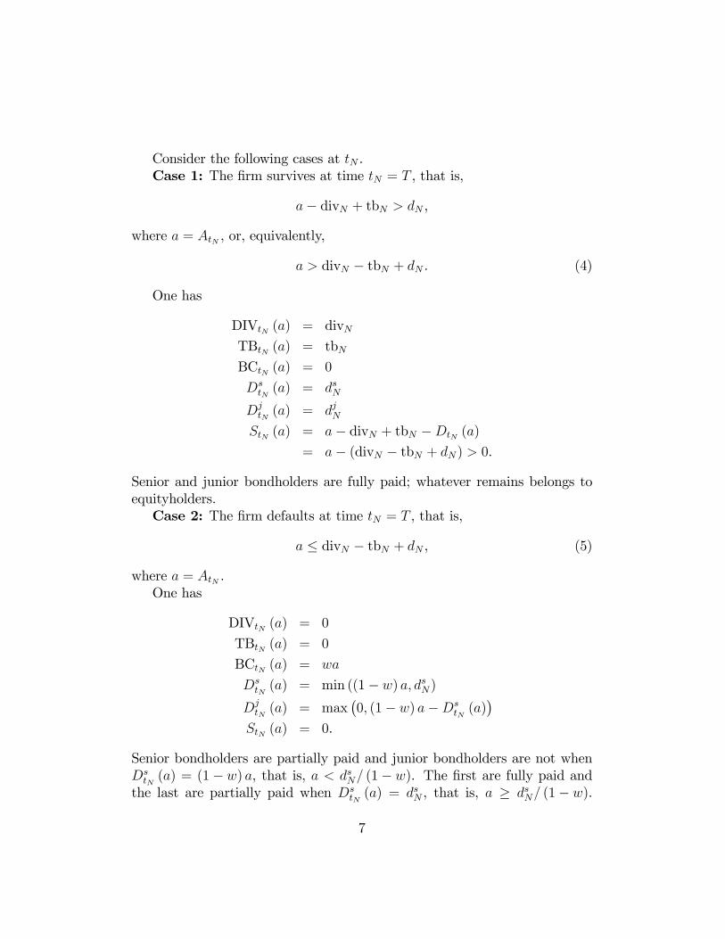
Consider the following cases at tN .Case 1: The �rm survives at time tN = T , that is,

a� divN + tbN > dN ,

where a = AtN , or, equivalently,

a > divN � tbN + dN . (4)

One has

DIVtN (a) = divNTBtN (a) = tbNBCtN (a) = 0

DstN(a) = dsN

DjtN(a) = djN

StN (a) = a� divN + tbN �DtN (a)

= a� (divN � tbN + dN) > 0.

Senior and junior bondholders are fully paid; whatever remains belongs toequityholders.Case 2: The �rm defaults at time tN = T , that is,

a � divN � tbN + dN , (5)

where a = AtN .One has

DIVtN (a) = 0

TBtN (a) = 0

BCtN (a) = wa

DstN(a) = min ((1� w) a; dsN)

DjtN(a) = max

�0; (1� w) a�Ds

tN(a)�

StN (a) = 0.

Senior bondholders are partially paid and junior bondholders are not whenDstN(a) = (1� w) a, that is, a < dsN= (1� w). The �rst are fully paid and

the last are partially paid when DstN(a) = dsN , that is, a � dsN= (1� w).

7

Clearly, all value functions at maturity are functions of AtN = a, and thebalance-sheet equality holds in all cases. We can do more, and explicit themas functions of a = AtN , e.g., StN (a) = max (0; a� (divn � tbN + dN)), forall a > 0. Thus, the stock can be seen as a call option (Merton 1974) fromthe perspective of an investor at time t 2 (tN�1; tN). This is not really helpfulhere; our approach is designed to accommodate any derivative whose valueat time t 2 [0; T ] is in the form � (t; a), where a = At.Suppose now that Ds

tn+1(:), Dj

tn+1 (:), and Stn+1 (:) are functions of a =Atn+1 at a certain future date tn+1, and that the balance-sheet equality holds.For t 2 (tn; tn+1), and consequently just after the payment date tn, no-arbitrage pricing gives

DIVt+n (a) = E��e�rf (tn+1�tn)DIVtn+1

�Atn+1

�j At+n = a

�(6)

TBt+n (a) = E��e�rf (tn+1�tn)TBtn+1

�Atn+1

�j At+n = a

�BCt+n (a) = E�

�e�rf (tn+1�tn)BCtn+1

�Atn+1

�j At+n = a

�Dst+n(a) = E�

�e�rf (tn+1�tn)Ds

tn+1

�Atn+1

�j At+n = a

�Dj

t+n(a) = E�

�e�rf (tn+1�tn)Dj

tn+1

�Atn+1

�j At+n = a

�St+n (a) = E�

�e�rf (tn+1�tn)Stn+1

�Atn+1

�j At+n = a

�,

where rf is the risk-free rate and At+n = a = Atn. As stated by Black and Cox(1976), debt cannot be �nanced by selling part of the �rm�s assets; rather,it is �nanced by issuing new shares of stock. This covenant applies here.Equation (6) implicitly assumes that the �rm survives for all t 2 (tn; tn+1)and a = At > 0, which is obviously true since

P ��Stn+1

�Atn+1

�> 0 j At = a

�> 0.

Technically, Black and Cox�s assumption results in a discontinuity at tn 2 Pof the value functions Dt (a) and St (a), seen as functions of t. Clearly,all value functions at t+n depend on a = At+n = Atn. Now, the martingaleproperty of the discounted state process fAg reduces to the balance-sheetequality at time t 2 (tn; tn+1), and consequently at t+n :

E����Atn+1 �DIVtn+1

�Atn+1

�+ TBtn+1

�Atn+1

�� BCtn+1

�Atn+1

��j

At+n = a�

= a�DIVt+n (a) + TBt+n (a)� BCt+n (a)= E�

���Dtn+1

�Atn+1

�+ Stn+1

�Atn+1

��j At+n = a

�= Dt+n

(a) + St+n (a) ,

8

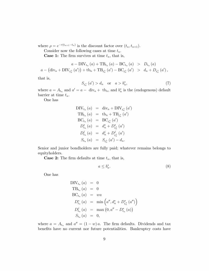
where � = e�r(tn+1�tn) is the discount factor over (tn; tn+1).Consider now the following cases at time tn.Case 1: The �rm survives at time tn, that is,

a�DIVtn (a) + TBtn (a)� BCtn (a) > Dtn (a)

a��divn +DIVt+n (a

0)�+ tbn + TBt+n (a

0)� BCt+n (a0) > dn +Dt+n

(a0) ,

that is,St+n (a

0) > dn or a > b�n, (7)

where a = Atn and a0 = a� divn + tbn, and b�n is the (endogenous) default

barrier at time tn.One has

DIVtn (a) = divn +DIVt+n (a0)

TBtn (a) = tbn + TBt+n (a0)

BCtn (a) = BCt+n (a0)

Dstn (a) = dsn +D

st+n(a0)

Djtn (a) = djn +D

j

t+n(a0)

Stn (a) = St+n (a0)� dn.

Senior and junior bondholders are fully paid; whatever remains belongs toequityholders.Case 2: The �rm defaults at time tn, that is,

a � b�n. (8)

One has

DIVtn (a) = 0

TBtn (a) = 0

BCtn (a) = wa

Dstn (a) = min

�a00; dsn +D

st+n(a00)

�Djtn (a) = max

�0; a00 �Ds

tn (a)�

Stn (a) = 0,

where a = Atn and a00 = (1� w) a. The �rm defaults. Dividends and tax

bene�ts have no current nor future potentialities. Bankruptcy costs have

9

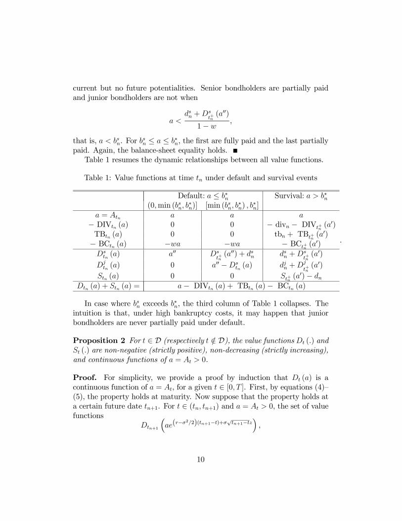
current but no future potentialities. Senior bondholders are partially paidand junior bondholders are not when

a <dsn +D

st+n(a00)

1� w ,

that is, a < bsn. For bsn � a � b�n, the �rst are fully paid and the last partially

paid. Again, the balance-sheet equality holds.Table 1 resumes the dynamic relationships between all value functions.

Table 1: Value functions at time tn under default and survival events

Default: a � b�n Survival: a > b�n(0;min (bsn; b

�n)] [min (bsn; b

�n) ; b

�n]

a = Atn a a a� DIVtn (a) 0 0 � divn � DIVt+n (a

0)TBtn (a) 0 0 tbn + TBt+n (a

0)� BCtn (a) �wa �wa � BCt+n (a

0)

Dstn (a) a00 Ds

t+n(a00) + dsn dsn +D

st+n(a0)

Djtn (a) 0 a00 �Ds

tn (a) djn +Dj

t+n(a0)

Stn (a) 0 0 St+n (a0)� dn

Dtn (a) + Stn (a) = a� DIVtn (a) + TBtn (a)� BCtn (a)

.

In case where bsn exceeds b�n, the third column of Table 1 collapses. The

intuition is that, under high bankruptcy costs, it may happen that juniorbondholders are never partially paid under default.

Proposition 2 For t 2 D (respectively t =2 D), the value functions Dt (:) andSt (:) are non-negative (strictly positive), non-decreasing (strictly increasing),and continuous functions of a = At > 0.

Proof. For simplicity, we provide a proof by induction that Dt (a) is acontinuous function of a = At, for a given t 2 [0; T ]. First, by equations (4)�(5), the property holds at maturity. Now suppose that the property holds ata certain future date tn+1. For t 2 (tn; tn+1) and a = At > 0, the set of valuefunctions

Dtn+1

�ae(r��

2=2)(tn+1�t)+�ptn+1�tz

�,

10

seen as functions of z 2 R, are bounded byNX

m=n+1

Bm.

By equation (6) and Lebesgue�s dominated Theorem (Cramér 1946), thevalue function Dt (:) is continuous:

lima!a0

Dt (a)

= lima!a0

ZRDtn+1

�ae(r��

2=2)(tn+1�t)+�ptn+1�tz

�e�r(tn+1�t)' (z) dz

=

ZRlima!a0

Dtn+1

�ae(r��

2=2)(tn+1�t)+�ptn+1�tz

�e�r(tn+1�t)' (z) dz

=

ZRDtn+1

�lima!a0

ae(r��2=2)(tn+1�t)+�

ptn+1�tz

�e�r(tn+1�t)' (z) dz

=

ZRDtn+1

�a0e(r��2=2)(tn+1�t)+�

ptn+1�tz

�e�r(tn+1�t)' (z) dz

= Dt (a0) ,

where the �rst two steps are due to Lebesgue�s dominated theorem, and thethree last steps are due to the continuity of the value function Dtn+1 (:).

Proposition 3 For t 2 [0; T ], the value function Dt (:) veri�es the additionalproperties

lima!0

Dt (a) = 0 and lima!1

Dt (a) =Mt =Xtn�t

e�(tn�t)rdn.

Thus, for a = At large enough at time t, the company is seen as risk free.

Proof. Again, we propose a proof by induction. First, we show that theproperty holds at maturity tN = T . Next, we assume that the propertyholds at a certain future date tn+1, and we show that it holds at t 2 (tn; tn+1),then at tn. Obviously, the property holds at tN = T (see equations (5)�(4).Suppose now that the property holds at tn+1. By equation (6), one has

Dt (a)

= E��e�rf (tn+1�t)Dtn+1

�Atn+1

�j At = a

�= E�

he�rf (tn+1�t)Dtn+1

�ae(r��

2=2)(tn+1�t)+�ptn+1�tZ

�i,

for t 2 (tn; tn+1) ,

11

where Z follows the standard normal distribution. Again, by the Lebesgue�sdominated Theorem and the continuity of Dtn+1 (:), one has

lima!0

Dt (a) = E�he�rf (tn+1�t) lim

a!0Dtn+1

�ae(r��

2=2)(tn+1�t)+�ptn+1�tZ

�i= 0,

and

lima!1

Dt (a) = E�he�rf (tn+1�t) lim

a!1Dtn+1

�ae(r��

2=2)(tn+1�t)+�ptn+1�tZ

�i= E�

�e�rf (tn+1�t)Mtn+1

�= e�rf (tn+1�t)Mtn+1,

where the last two steps come from the induction hypothesis at time tn+1.Clearly, the same result holds when t ! tn and t > tn. Finally, by equa-tion (8), one has

lima!0

Dtn (a) = 0,

and by equation (7), one has

lima!1

Dtn (a) = e�rf (tn+1�tn)Mtn+1 + dn

= Mtn.

The literature reports two de�nitions for the notion of default probability,one is unconditional and the other is conditional on lately survival. The(total) default probability up to time tn is

�n = P � (Default at t1 or . . . or Default at tn)

= P � ([ni=1 fAti � b�i g)= 1� P �

�[ni=1 fAti � b�i g

�= 1� P � (\ni=1 fAti > b�i g) ,= 1� P � (At1 > b�1; : : : ; Atn > b�n) , for n = 1; : : : ; N ,

and the conditional default probability up to time tn given lately survival till

12

tn�1 is

�cn = P � (Default at tn j Survival till tn�1)

=P ��At1 > b

�1; : : : ; Atn�1 > b

�n�1; Atn � b�n

�P ��At1 > b

�1; : : : ; Atn�1 > b

�n�1�

= 1� P � (At1 > b�1; : : : ; Atn > b

�n)

P ��At1 > b

�1; : : : ; Atn�1 > b

�n�1�

These default proportions can be computed under the risk-neutral and/orthe physical probability measure. Delianedis and Geske (2003) claim thatthe di¤erences over time in the risk-neutral default probabilities are powerfulpredictors of corporate bankruptcy. Thus, according to the authors, we canignore the drift parameter of the GBM state process fAg under the physicalprobability measure, known to carry a high estimation sampling error.Although less rigorous, the (total) default probabilities are generally pre-

ferred to the conditional default probabilities. The reason lies in the factthat conditional default probabilities, given lately survival, are informativeonly for the very near future. Given that the �rm survives under the struc-tural model at time t0 2 (t�0; t1), for all a = At0 > 0, a slightly high defaultprobability can be observed for the horizon t1. Later on, given survival attime tn, the �rm will likely to survive at time tn+1, essentially if the mostimportant payments (the principal amounts) are still due. This fact can bedrastically altered in the presence of a sinking fund.As well, we can de�ne the senior term structure of loss probabilities by

�n = 1� P � (At1 > min (bs1; b�1) ; : : : ; Atn > min (bsn; b�n)) ,

and

�cn = 1�P � (At1 > min (b

s1; b

�1) ; : : : ; Atn > min (b

sn; b

�n))

P ��At1 > min (b

s1; b

�1) ; : : : ; Atn�1 > min

�bsn�1; b

�n�1�� .

Proposition 4 Let fXg be a geometric Brownian motion with an initialposition X0, a drift �, a volatility �, and c1; : : : ; cn 2 R. One has

P (Xt1 > c1; : : : ; Xtn > cn) = � (c01; : : : ; c

0n) ,

where

c0m =log (X0=cm) + (�� �2=2) tm

�, for m = 1; : : : ; n,

13

and � (:) is the cumulative distribution function of the multivariate normallaw N (0;� = CCt) with

C =

266664pt1 � t0 0 0 0 0pt1 � t0

pt2 � t1 0 0 0

� � � � � � � � � 0 0pt1 � t0

pt2 � t1 � � � p

tn�1 � tn�2 0pt1 � t0

pt2 � t1 � � � p

tn�1 � tn�2ptn � tn�1

377775 .Proof. The proof is based on the fact that

Xtm

= X0e(���2=2)tm��Wtm

= X0e(���2=2)tm��(

pt1�t0Z1+���+

ptm�tm�1Zm),

where fWg is a standard Brownian motion, and (Z1; : : : ; Zn)t 2 Rn fol-lows the standard normal law N (0; In), where In is the identity variance-covariance matrix of size n. For m = 1; : : : ; n, the event

fXtm > cmg

is equivalent to npt1 � t0Z1 + � � �+

ptm � tm�1Zm � c0m

o,

that is, �The mth row of CZ � c0m

.

3 The Dynamic Program

Let G = fa1; : : : ; apg be a mesh of grid points for the value of the �rm, a0 = 0,and ap+1 =1. It is better for the grid points to be more concentrated wherethe value of the �rm is the most likely to happen and variate. The optimalchoice of G is not addressed here; however, the dynamic program proposedreaches any desired level of accuracy as long as a1 and ap are extreme enoughand ai+1 � ai, for i = 1; : : : ; p � 1, are small enough. At time tn 2 P,the quantiles of the state process fAg at time tn+1 can be used for grid

14

construction. To alleviate the notation, the mesh of grid points is indicatedby G instead of Gn.Suppose now that approximations of all value functions are available on

G at a certain future date tn+1. They are indicated by gDIVtn+1 (:), fTBtn+1 (:),fBCtn+1 (:), eDstn+1

(:), eDjtn+1 (:), and eStn+1 (:). This is not really a strong as-

sumption since the value functions are known in closed form at maturitytN = T . The dynamic program works as follows:

1. Start the program at m = n+1, where the value functions gDIVtn+1 (:),fTBtn+1 (:), fBCtn+1 (:), eDstn+1

(:), eDjtn+1 (:), and eStn+1 (:) are known on

G at tn+1. Then, interpolate these value functions, de�ned on G,using piecewise-linear polynomials, and compute the approximationsdDIVtn+1 (:), cTBtn+1 (:), cBCtn+1 (:), bDs

tn+1(:), bDj

tn+1 (:), and bStn+1 (:), de-�ned on the overall state space R�+.

2. Use equations (1)�(2), and compute in closed form the transition pa-rameters at time tn, that is, T 0kin = T

0akaiai+1�n

and T 1kin = T1akaiai+1�n

,where �n = tn+1 � tn.

3. Use equation (6) and compute the value functions eDst+n(:) and eSt+n (:)

on G.

4. For ak 2 G, search for k0 and k00 such that a0k = ak� divn+ tbn 2[ak0 ; ak0+1) and a00k = (1� w) ak 2 [ak00 ; ak00+1). Then, approximate a0kby ak0 and a00k by ak00, both in G.

5. Approximate the default barriers b�n and then bsn at tn as follows:

eb�n = minnak 2 G such that eSt+n (ak0) > dnoebsn = minnak 2 G such that (1� w) ak > eDs

t+n(ak00) + d

sn

o.

6. Use equation (6) and Table 1, and compute gDIVtn (:), fTBtn (:), fBCtn (:),eDstn (:),

eDjtn (:), and eStn (:) on G. Then, interpolate these value func-

tions, de�ned on G, using piecewise-linear polynomials, and computethe approximations dDIVtn (:), cTBtn (:), cBCtn (:), bDs

tn (:),bDjtn (:), andbStn (:), de�ned on the overall state space R�+.

15

7. If m� 1 = n = 0, stop the program; else set m =: m� 1, go to step 1,and repeat.

For a value function v (:), Step 1 can be written as follows:

bvtn+1 (a) = pXi=0

�v�n+1i +v �n+1i a

�I (ai � a < ai+1) ,

where the internal local coe¢ cients v�n+1i and v�n+1i , for i = 1; : : : ; p� 1, are

v�n+1i =evtn+1 (ai+1)� evtn+1 (ai)

ai+1 � aiv�n+1i =

ai+1evtn+1 (ai)� aievtn+1 (ai+1)ai+1 � ai

,

and the external local coe¢ cients are set to the values of their adjacentintervals, that is, �

v�n+10 ;v �n+10

�=�v�n+11 ;v �n+11

�,

and �v�n+1p ;v �n+1p

�=�v�n+1p�1 ;

v �n+1p�1�.

Step 3 can be written as

evt+n (ak) = E��e�rf (tn+1�tn)bvtn+1 �Atn+1� j Atn = ak� (9)

= e�rf (tn+1�tn)pXi=0

�v�n+1i T 0kin +

v �n+1i T 1kin�,

for k = 1; : : : ; p ,

whether the function v (:) represents Ds (:) or S (:).The transition parameters are known in closed formwhen the state process

moves according to a GBM (Ben-Ameur, Breton, and François 2004). Fi-nally, from (9), all value functions just after a payment date can be writtenas a sum of local future values multiplied by their associated transition pa-rameters given the current position of the state process. This sum of smallpieces is then discounted back at the risk-free rate. The transition tables in(1)�(2) play a major role for this dynamic program to run. This procedurecan be improved further by using the transition tables T 2 or T 2 and T 3, thatis, mixing between the dynamic program and piecewise quadratic or cubic

16

polynomials, but the gain in accuracy will mostly be o¤set by the loss incomputing time.The code is written in the C language, compiled with the GCC compiler,

and run under Windows 7 (64 bits). The GSL library (Galassi et al. 2009)is used to achieve speci�c computing tasks, and the CUBATURE softwarepackage (Hahn 2005) to compute default probabilities by numerical integra-tion.

4 Model-Estimation Step

The model-estimation step combines the historical approach and the implicitapproach. The notation used here is independent of the one used in theprevious sections. Let A�n; : : : ; A0 be a time series taken from the stateprocess fAg, and observed at regular dates t�n; : : : ; t0, where � = t�m+1 �t�m is a real constant. For our empirical investigation, we experiment withseveral values of �, and take one week (� = 1=52 years). The estimates arerobust.The random sample of log-returns on the value of the �rm under the

physical probability measure, that is, R�n = ln (A�n+1=A�n) ; : : : ; R�1 =ln (A0=A�1), is independent and identically distributed. The common distri-bution is the normal law

Nh��� �2=2

��;p��i.

The following results come:

E [R�m] =��� �2=2

�� and V [R�m] = ��

2,

for m = 1; : : : ; n. The method of moments is used here to estimate theunknown parameters (�; �) as follows:

b� = SRp�

and b� = R + S2R=2

�, (10)

where R and SR are the sample mean and the sample standard deviation ofRm = ln (A�m+1=A�m).For � small enough, the model-estimation step works as follows:

1. For iteration p = 0, set A(p)�m = Aaccounting�m , for m = 0; : : : ; n;

17

2. Use equation (10), and estimate the unknown parameters at iterationp, that is, b�(p) and b�(p);

3. Run the dynamic program (DP) and approximate the value of equitytime series at iteration p, that is,

S(p)�n; : : : ; S

(p)0 ;

4. Compare the DP values of the stock at iteration p with their associatedmarket prices

Smarket�n ; : : : ; Smarket0 ;

5. If maxm����S(p)�m � Smarket�m

�=Smarket�m

��� < � then stop;6. Else adjust each approximated value of the �rm A

(p)�m towards its im-

plicit valueA(p)�m ! Aimplicit�m , for m = 0; : : : ; n,

set p = p+ 1, and go to step 2.

At Step 3, DP is run with a grid size of 2000. At step 6, the fact thatS�m is an increasing function of A�m, for m = 1; : : : ; n, helps to adjust thetime series A(p)�m; : : : ; A

(p)�0 in the right direction(s). The empirical investiga-

tion, performed on selected public North American companies, shows fullconvergence at around 6 iterations.

5 A Numerical Investigation

The objective of this numerical investigation is twofold. First of all, we com-pare DP values to selected closed-form solutions found in the literature, andshow that DP approach is a viable alternative to the analytical approach. DPis convergent, e¢ cient, and robust. Next, we replicate and comment selectedFigures from the literature. These are sensibility analysis that representstylized �nancial �ndings.Table 1 is based on information from Nivorozhkin (2005b), and compares

DP values to Black and Cox (1976). Set T = 1 (year), N = 1 (period),At0 = $100, Bs1 = $70, Bj1 = $30, and rf = 10% (per year). This is aportfolio of a senior pure bond and a junior pure bond, both maturing in oneyear. B&C stands for Black and Cox.

18

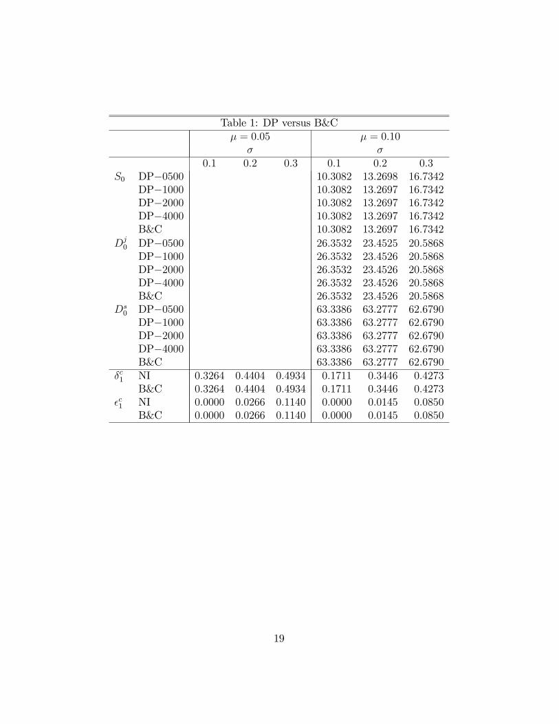
Table 1: DP versus B&C� = 0:05 � = 0:10

� �0:1 0:2 0:3 0:1 0:2 0:3

S0 DP�0500 10:3082 13:2698 16:7342DP�1000 10:3082 13:2697 16:7342DP�2000 10:3082 13:2697 16:7342DP�4000 10:3082 13:2697 16:7342B&C 10:3082 13:2697 16:7342

Dj0 DP�0500 26:3532 23:4525 20:5868DP�1000 26:3532 23:4526 20:5868DP�2000 26:3532 23:4526 20:5868DP�4000 26:3532 23:4526 20:5868B&C 26:3532 23:4526 20:5868

Ds0 DP�0500 63:3386 63:2777 62:6790DP�1000 63:3386 63:2777 62:6790DP�2000 63:3386 63:2777 62:6790DP�4000 63:3386 63:2777 62:6790B&C 63:3386 63:2777 62:6790

�c1 NI 0:3264 0:4404 0:4934 0:1711 0:3446 0:4273B&C 0:3264 0:4404 0:4934 0:1711 0:3446 0:4273

�c1 NI 0:0000 0:0266 0:1140 0:0000 0:0145 0:0850B&C 0:0000 0:0266 0:1140 0:0000 0:0145 0:0850

19

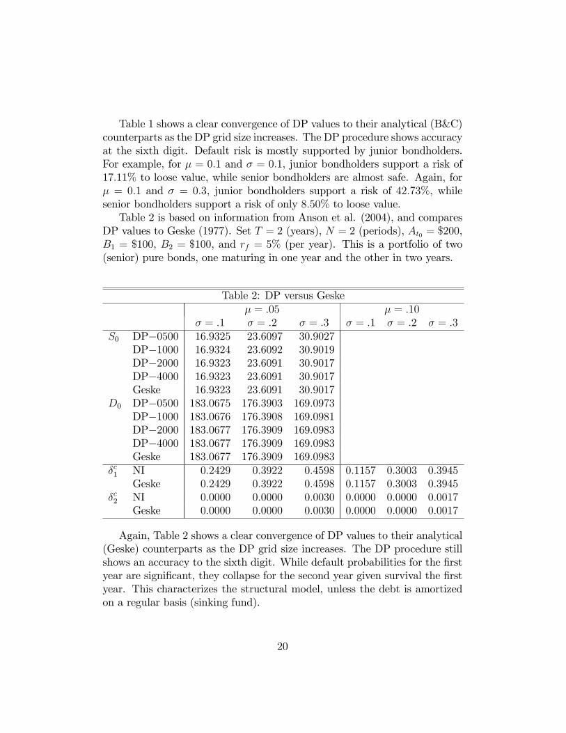
Table 1 shows a clear convergence of DP values to their analytical (B&C)counterparts as the DP grid size increases. The DP procedure shows accuracyat the sixth digit. Default risk is mostly supported by junior bondholders.For example, for � = 0:1 and � = 0:1, junior bondholders support a risk of17:11% to loose value, while senior bondholders are almost safe. Again, for� = 0:1 and � = 0:3, junior bondholders support a risk of 42:73%, whilesenior bondholders support a risk of only 8:50% to loose value.Table 2 is based on information from Anson et al. (2004), and compares

DP values to Geske (1977). Set T = 2 (years), N = 2 (periods), At0 = $200,B1 = $100, B2 = $100, and rf = 5% (per year). This is a portfolio of two(senior) pure bonds, one maturing in one year and the other in two years.

Table 2: DP versus Geske� = :05 � = :10

� = :1 � = :2 � = :3 � = :1 � = :2 � = :3S0 DP�0500 16:9325 23:6097 30:9027

DP�1000 16:9324 23:6092 30:9019DP�2000 16:9323 23:6091 30:9017DP�4000 16:9323 23:6091 30:9017Geske 16:9323 23:6091 30:9017

D0 DP�0500 183:0675 176:3903 169:0973DP�1000 183:0676 176:3908 169:0981DP�2000 183:0677 176:3909 169:0983DP�4000 183:0677 176:3909 169:0983Geske 183:0677 176:3909 169:0983

�c1 NI 0:2429 0:3922 0:4598 0:1157 0:3003 0:3945Geske 0:2429 0:3922 0:4598 0:1157 0:3003 0:3945

�c2 NI 0:0000 0:0000 0:0030 0:0000 0:0000 0:0017Geske 0:0000 0:0000 0:0030 0:0000 0:0000 0:0017

Again, Table 2 shows a clear convergence of DP values to their analytical(Geske) counterparts as the DP grid size increases. The DP procedure stillshows an accuracy to the sixth digit. While default probabilities for the �rstyear are signi�cant, they collapse for the second year given survival the �rstyear. This characterizes the structural model, unless the debt is amortizedon a regular basis (sinking fund).

20

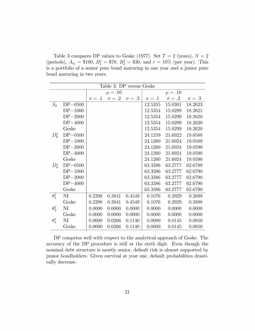
Table 3 compares DP values to Geske (1977). Set T = 2 (years), N = 2(periods), At0 = $100, B

s1 = $70, B

j2 = $30, and r = 10% (per year). This

is a portfolio of a senior pure bond maturing in one year and a junior purebond maturing in two years.

Table 3: DP versus Geske� = :05 � = :10

� = :1 � = :2 � = :3 � = :1 � = :2 � = :3S0 DP�0500 12:5355 15:0301 18:2623

DP�1000 12:5354 15:0299 18:2621DP�2000 12:5354 15:0299 18:2620DP�4000 12:5354 15:0299 18:2620Geske 12:5354 15:0299 18:2620

Dj0 DP�0500 24:1259 21:6922 19:0588DP�1000 24:1260 21:6924 19:0589DP�2000 24:1260 21:6924 19:0590DP�4000 24:1260 21:6924 19:0590Geske 24:1260 21:6924 19:0590

Ds0 DP�0500 63:3386 63:2777 62:6789DP�1000 63:3386 63:2777 62:6790DP�2000 63:3386 63:2777 62:6790DP�4000 63:3386 63:2777 62:6790Geske 63:3386 63:2777 62:6790

�j1 NI 0:2298 0:3841 0:4549 0:1076 0:2929 0:3898Geske 0:2298 0:3841 0:4549 0:1076 0:2929 0:3898

�j2 NI 0:0000 0:0000 0:0000 0:0000 0:0000 0:0000Geske 0:0000 0:0000 0:0000 0:0000 0:0000 0:0000

�s1 NI 0:0000 0:0266 0:1140 0:0000 0:0145 0:0850Geske 0:0000 0:0266 0:1140 0:0000 0:0145 0:0850

DP competes well with respect to the analytical approach of Geske. Theaccuracy of the DP procedure is still at the sixth digit. Even though thenominal debt structure is mostly senior, default risk is almost supported byjunior bondholders. Given survival at year one, default probabilities drasti-cally decrease.

21

6 An Empirical Investigation

The objective of this empirical section is to apply our DP framework to a setof two North American public companies, Bally Total Fitness Holding Corp.(BTFH) and Hudson Bay Company (HBC). The �rst �rm experienced �nan-cial di¢ culties in the past 5 years, while the second one is considered healthywith solid �nancial indicators. We value their corporate bond portfolios, es-timate their corresponding equity value, and assess their term structure ofdefault probabilities. For each company, we use complete accounting, �nan-cial, and market information such us balance sheets (and related footnotes),income statements, and stock market data (including dividend distributions).This information is obtained from various sources such as Edgar, Compustat,and CRSP databases.

6.1 Bally Total Fitness Holding Corp. (BTFH)

BTFH is a well known US company in the �tness industry created in the1930s. Its �nancial statements show poor �nancial performance during theperiod 2002-2005 with a notable impact on its shareholders� equity. Suchsituation is explained by �erce competition and severe �nancing problemsas re�ected by the �rm�s inability to properly manage its liabilities. Forinstance, all of its liquidity indicators such as current ratios are constantlybelow 0.40 and where short-term liabilities represent 40% of total liabili-ties over the same period. The persistent negative trend in these �nancialstatistics would imply future �nancial di¢ culties for BTFH.Our estimation of the default probabilities and other relevant measures

are reported in Table 4.2 over a period of six years. It takes into consider-ation the existence of junior and senior debts in the structure of the �rm�sliabilities. All of default probabilities are quiet high and range from 0.71 to0.99 for a one-year default horizon. These DP estimates compare well withthe aggregate measures of Merton (1974) and Geske (1977). Our results arecon�rmed when in late 2008, BTFH �led for Chapter 11 bankruptcy protec-tion for the second time in less than two years, caused by debt and limitedre�nancing options during last credit crisis. When the default horizon in-creases, the probabilities vanish and are close to zero with few exceptions in2004 and 2005. For example, the probability of default in three years givenno default in the previous two years is 0.41 in 2004. In all cases, the loss tosenior debtholders is negligible.

22

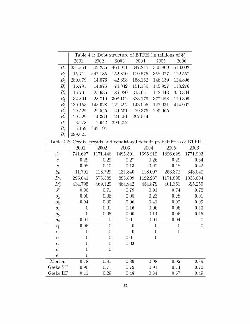
Table 4.1: Debt structure of BTFH (in millions of $)2001 2002 2003 2004 2005 2006

Bj1 331:864 309:235 460:911 347:215 330:809 510:092

Bj2 15:711 347:185 152:810 129:575 358:077 122:557

Bj3 280:079 14:876 42:698 158:162 146:139 124:896

Bj4 16:791 14:876 74:042 151:139 145:927 118:276

Bj5 16:791 25:635 86:920 315:651 142:443 353:304

Bj6 32:894 28:719 308:102 383:179 377:498 119:399Bs1 139:158 148:028 121:492 143:005 127:931 414:907Bs2 29:529 29:545 29:551 29:375 295:905Bs3 29:529 14:369 29:551 297:514Bs4 8:978 7:642 299:252Bs5 5:159 299:194Bs6 299:025

Table 4.2: Credit spreads and conditional default probabilities of BTFH2001 2002 2003 2004 2005 2006

A0 741:627 1171:446 1485:591 1695:212 1826:628 1771:903� 0:29 0:29 0:27 0:26 0:29 0:34� 0:08 �0:10 �0:13 �0:22 �0:18 �0:22S0 11:791 128:729 131:840 118:097 253:372 343:040

Dj0 295:041 573:588 888:809 1122:237 1171:895 1033:604

Ds0 434:795 469:129 464:942 454:879 401:361 395:259�c1 0:90 0:71 0:79 0:91 0:74 0:72�c2 0:00 0:06 0:05 0:23 0:28 0:01�c3 0:04 0:00 0:06 0:41 0:02 0:09�c4 0 0:01 0:16 0:06 0:06 0:13�c5 0 0:05 0:00 0:14 0:06 0:15�c6 0:01 0 0:01 0:01 0:04 0�c1 0:06 0 0 0 0 0�c2 0 0 0 0 0�c3 0 0 0:01 0�c4 0 0 0:03�c5 0 0�c6 0

Merton 0:78 0:81 0:89 0:98 0:92 0:89Geske ST 0:90 0:71 0:79 0:91 0:74 0:72Geske LT 0:11 0:29 0:48 0:84 0:67 0:49

23

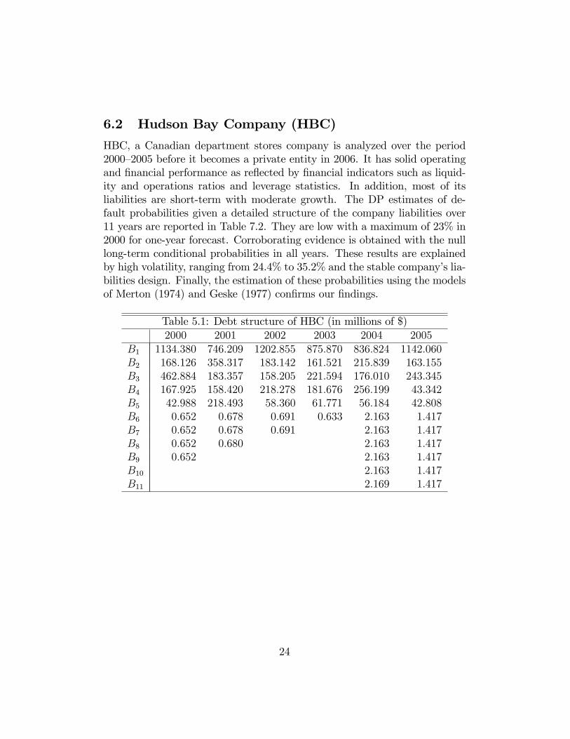
6.2 Hudson Bay Company (HBC)

HBC, a Canadian department stores company is analyzed over the period2000�2005 before it becomes a private entity in 2006. It has solid operatingand �nancial performance as re�ected by �nancial indicators such as liquid-ity and operations ratios and leverage statistics. In addition, most of itsliabilities are short-term with moderate growth. The DP estimates of de-fault probabilities given a detailed structure of the company liabilities over11 years are reported in Table 7.2. They are low with a maximum of 23% in2000 for one-year forecast. Corroborating evidence is obtained with the nulllong-term conditional probabilities in all years. These results are explainedby high volatility, ranging from 24.4% to 35.2% and the stable company�s lia-bilities design. Finally, the estimation of these probabilities using the modelsof Merton (1974) and Geske (1977) con�rms our �ndings.

Table 5.1: Debt structure of HBC (in millions of $)2000 2001 2002 2003 2004 2005

B1 1134:380 746:209 1202:855 875:870 836:824 1142:060B2 168:126 358:317 183:142 161:521 215:839 163:155B3 462:884 183:357 158:205 221:594 176:010 243:345B4 167:925 158:420 218:278 181:676 256:199 43:342B5 42:988 218:493 58:360 61:771 56:184 42:808B6 0:652 0:678 0:691 0:633 2:163 1:417B7 0:652 0:678 0:691 2:163 1:417B8 0:652 0:680 2:163 1:417B9 0:652 2:163 1:417B10 2:163 1:417B11 2:169 1:417

24

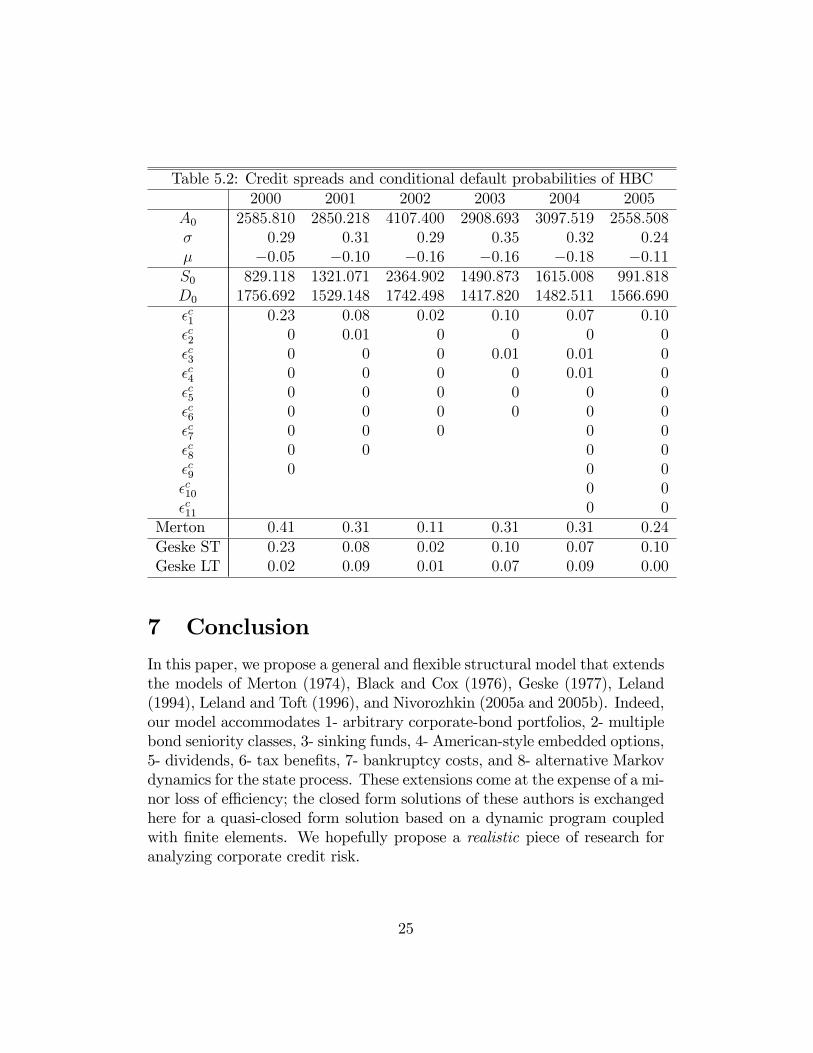
Table 5.2: Credit spreads and conditional default probabilities of HBC2000 2001 2002 2003 2004 2005

A0 2585:810 2850:218 4107:400 2908:693 3097:519 2558:508� 0:29 0:31 0:29 0:35 0:32 0:24� �0:05 �0:10 �0:16 �0:16 �0:18 �0:11S0 829:118 1321:071 2364:902 1490:873 1615:008 991:818D0 1756:692 1529:148 1742:498 1417:820 1482:511 1566:690�c1 0:23 0:08 0:02 0:10 0:07 0:10�c2 0 0:01 0 0 0 0�c3 0 0 0 0:01 0:01 0�c4 0 0 0 0 0:01 0�c5 0 0 0 0 0 0�c6 0 0 0 0 0 0�c7 0 0 0 0 0�c8 0 0 0 0�c9 0 0 0�c10 0 0�c11 0 0

Merton 0:41 0:31 0:11 0:31 0:31 0:24Geske ST 0:23 0:08 0:02 0:10 0:07 0:10Geske LT 0:02 0:09 0:01 0:07 0:09 0:00

7 Conclusion

In this paper, we propose a general and �exible structural model that extendsthe models of Merton (1974), Black and Cox (1976), Geske (1977), Leland(1994), Leland and Toft (1996), and Nivorozhkin (2005a and 2005b). Indeed,our model accommodates 1- arbitrary corporate-bond portfolios, 2- multiplebond seniority classes, 3- sinking funds, 4- American-style embedded options,5- dividends, 6- tax bene�ts, 7- bankruptcy costs, and 8- alternative Markovdynamics for the state process. These extensions come at the expense of a mi-nor loss of e¢ ciency; the closed form solutions of these authors is exchangedhere for a quasi-closed form solution based on a dynamic program coupledwith �nite elements. We hopefully propose a realistic piece of research foranalyzing corporate credit risk.

25

Our numerical investigation shows e¢ ciency, convergence, and robust-ness. All in all, we discover the same results reported in the literature on 1-the endogenous default barriers, 2- the maximum debt capacity, 3- the opti-mal capital structure, 4- the properties of the debt and equity value functions,and 5- the term structure of (unconditional and conditional) default proba-bilities. Nonetheless, we observe a small gap between our results with respectto Leland (1994) (in presence of frictions). This gap is explained by the factthat Leland transfers the overall impact of the frictions on the �rm�s assetsat the origin, and assumes that these frictions impact equity but not debt.More realistically, frictions in our dynamic model impact the �rm�s assetsat each payment date, while the economic balance-sheet equality holds, andimpact both debt and equity.Future research avenues consist of integrating: 1- options embedded in

corporate bonds, 2- reorganization/liquidation processes, 3- alternative dy-namics for the state process, and 4- multidimensional state processes.Acknowledgements: This research has been supported by Brock Uni-

versity advancement fund for the �rst author, and NSERC and IFM2 for thesecond author.

References

[1] Anderson, W.A., and S. Sundaresan, 1996, �Design and Valuation ofDebt Contracts,�Review of Financial Studies, 9, 37�68.

[2] Anson, M.J.P., F.J. Fabozzi, M. Choudhry, and R. Chen, 2004, CreditDerivatives: Instruments Applications, and Pricing, JohnWiley & Sons,Inc., New Jersey.

[3] Aziz, M.A., and H.A. Dar, 2006, �Predicting Corporate Bankruptcy:Where We Stand?,�Corporate Governance, 6, 18�33.

[4] Ben-Ameur, H., M. Breton, and J.-M. Martinez, 2009, �A Dynamic-Programming Approach for Pricing Derivatives in the GARCH Model,�Management Science, 55, 252�266.

[5] Ben-Ameur, H., M. Breton, L. Karoui, and P. L�Écuyer, 2007, �ADynamic Programming Approach for Pricing Options Embedded inBonds,�Journal of Economic Dynamics and Control, 31, 2212�2233.

26

[6] Ben-Ameur, H., M. Breton, and P. François, 2004, �A Dynamic Pro-gramming Approach to Price Installment Options,�European Journalof Operational Research, 169, 667�676.

[7] Ben-Ameur, H., M. Breton, and P. L�Écuyer, 2002, �A Dynamic Pro-gramming Procedure for Pricing American-style Asian Options,�Man-agement Science, 48, 625�643.

[8] Ben-Ameur, H., R. Chérif, and B. Remillard, 2012, �A Dynamic Pro-gramming Approach for Valuing Derivatives under Jump-Di¤usion,�Cahier du GERAD no ???.

[9] Benos, A., and G. Papanastasopoulos, 2007, �Extending the MertonModel: A Hybrid Approach to Assessing Credit Quality,�Mathematicaland Computer Programming, 46, 47�68.

[10] Black, F., and J.C. Cox, 1976, �Valuing Corporate Securities: SomeE¤ects of Bond Indenture Provisions,�Journal of Finance, 31, 351�367.

[11] Black, F., and M. Scholes, 1973, �The Pricing of Options and CorporateLiabilities,�Journal of Political Economy, 81, 637�654.

[12] Broadie, M., M. Chernov, S. Sundaresan, 2007, �Optimal Debt andEquity Values in the Presence of Chapter 7 and Chapter 11,�Journalof Finance, 62, 1341�1377.

[13] Chen, N., and S.G. Kou, 2009, �Credit Spreads, Optimal Capital Struc-ture, and Implied Volatility with Endogenous Default and Jump Risk,�Mathematical Finance, 19, 343�378.

[14] Collin-Dufresne, P., and R. Goldstein, 2001, �Do Credit Spreads Re�ectStationary Leverage Ratios?,�Journal of Finance, 56, 1929�1957.

[15] Cramér, H., 1946, Mathematical Models of Statistics, Princeton Univer-sity Press, New Jersey.

[16] Delianedis, G., and R. Geske, 2003, Credit Risk and Risk Neutral De-fault Probabilities: Information about Rating Migrations and Defaults,Working Paper, The Anderson School at UCLA.

27

[17] Delianedis, G., and R. Geske, 2001, The Components of CorporateCredit Spreads: Default, Recovery, Tax, Jumps, Liquidity, and Mar-ket Factors, Working Paper, The Anderson School at UCLA.

[18] Ericsson, J., and J. Reneby, 1998, �A Framework for Valuing CorporateSecurities,�Applied Mathematical Finance, 5, 143�163.

[19] François, P., and E. Morellec, 2004, �Capital Structure and Asset Prices:Some E¤ects of Bankruptcy Procedures,�Journal of Business, 77, 387�412.

[20] Galai, D., A. Raviv, and Z. Wiener, 2007, �Liquidation Triggers andThe Valuation of Equity and Debt,�Journal of Banking and Finance,31, 3604�3620.

[21] Galassi, M., J. Davies, J. Theiler, B. Gough, G. Jungman, P. Alken, M.Booth, and F. Rossi, 2009, GNU Scienti�c Library Reference Manual,Network Theory Ltd., London.

[22] Geske, R., 1977, �The Valuation of Corporate Liabilities as CompoundOptions,�Journal of Financial and Quantitative Analysis, 12, 541�552.

[23] Hahn, T., 2005, �CUBA-a library for multidimensional numerical inte-gration,�Computer Physics Communications, 168, 78�95.

[24] Hillegeist, S., E. Keating, D. Cram, and K. Lundstedt, 2004, �Assessingthe Probability of Bankruptcy,�Review of Accounting Studies, 9, 5�34.

[25] Hsu, J.C., J. Saá-Requejo, and P. Santa-Clara, 2010, �A StructuralModel of Default Risk,�Journal of Fixed Income, 19, 77�94.

[26] Huang, J.-Z., andM. Huang, 2003, HowMuch of the Corporate-TreasuryYield Spread is Due to Credit Risk? Working Paper, Penn State Uni-versity, New York University, and Stanford University.

[27] Leland, H.E., 1994, �Corporate Debt Value, Bond Covenants and Opti-mal Capital Structure,�Journal of Finance, 49, 1213�1252.

[28] Leland, H.E., 2004, �Predictions of Default Probabilities in StructuralModels of Debt,�Journal of Investment Management, 2, 5�20.

28

[29] Leland, H.E., and K.B. Toft, 1996, �Optimal Capital Structure, Endoge-nous Bankruptcy and the Term Structure of Credit Spreads,�Journalof Finance, 51, 987�1019.

[30] Longsta¤, F.A., and E.S. Schwartz, 1995, �A Simple Approach to Valu-ing Risky Fixed and Floating Rate Debt,�Journal of Finance, 50, 789�819.

[31] Merton, R., 1974, �On the Pricing of Corporate Debt: The Risk Struc-ture of Interest Rates,�Journal of Finance, 29, 449�470.

[32] Miller, M.H., 1977, �Debt and Taxes,�Journal of Finance, 32, 261�275.

[33] Nivorozhkin, E., 2005a, �The Informational Content of SubordinatedDebt and Equity Prices in the Presence of Bankruptcy Costs,�EuropeanJournal of Operational Research, 163, 94�101.

[34] Nivorozhkin, E., 2005b, �Market Discipline of Subordinated Debt inBanking: The Case of Costly Bankruptcy,�European Journal of Oper-ational Research, 161, 364�376.

[35] Suo, W., and W. Wang, 2006, Assessing Default Probabilities fromStructural Credit Risk Models, Working Paper, Queen�s School of Busi-ness.

[36] Zhou, C., 2001, �The Term Structure of Credit Spreads with JumpRisk,�Journal of Banking and Finance, 25, 2015�2040.

29