Embed Size (px)
Citation preview
A DYNAMIC SIMULATOR FOR THE MANAGEMENT OF DISORDERS OF THE
BODY WATER METABOLISM
by
Özge Karanfil
B.S., Industrial Engineering, Boğaziçi University, 2002
Submitted to the Institute for Graduate Studies in
Science and Engineering in partial fulfillment of
the requirements for the degree of
Master of Science
Graduate Program in Industrial Engineering
Boğaziçi University
2005
ii
A DYNAMIC SIMULATOR FOR THE MANAGEMENT OF DISORDERS OF THE
BODY WATER METABOLISM
APPROVED BY:
Prof. Yaman Barlas …………………………
(Thesis Supervisor)
Assist. Prof. Aybek Korugan …………………………
Assoc. Prof. Ahmet Ademoğlu …………………………
DATE OF APPROVAL: 15.09.2005
iii
ACKNOWLEDGEMENT
I would like to express my deepest gratitude to Prof. Yaman Barlas, my thesis
supervisor, for his invaluable guidance and support throughout all phases of this research,
and for his patience.
I would like to thank Assoc. Prof. Ahmet Ademoğlu and Assist. Prof. Aybek
Korugan for taking part in my thesis committee and providing valuable comments for my
further research.
I wish to express my deepest gratitude to my parents, Gül and Hüseyin Karanfil and
to my sister Simge Karanfil, for their never ending support and affection.
I finally wish to thank all of my friends for being with me, especially in my last two
years. I am also thankful to the members of Sesdyn Research Group for their great
understandings and supports during my study.
iv
ABSTRACT
A DYNAMIC SIMULATOR FOR THE MANAGEMENT OF
DISORDERS OF THE BODY WATER METABOLISM
Regulation of the body water and its appropriate distribution between compartments
necessitates an understanding of two homeostatic systems: the system that regulates the
extracellular (EC) sodium concentration/body water content and the system that regulates
the blood volume/sodium content. The main feedback system for body water regulation is
the Antidiuretic Hormone (ADH)-thirst system, and the main feedback mechanisms for
sodium balance include the Aldosterone and the Atrial Natriuretic Hormones, and the renal
mechanisms. In ADH-induced hyponatremia, both the ADH and the thirst feedback loops
are dysregulated, and the result is a lower sodium concentration and higher body water
content, which may cause serious consequences.
In this study, a simulation model is built using system dynamics methodology to
study the body water regulation and its disorders by focusing on the fundamental feedback
mechanisms in the normal and disease physiology. This model is then extended to include
related therapeutic interventions of a particular body water disorder, namely water
intoxication/ hyponatremia, and a game version is produced to test the possible effects of a
given set of treatment options on a simulated patient. The model is shown to adequately
reproduce the changes in the body fluid balance not only in a normal person as a result of a
given disturbance, but also in a hypothetical hyponatremia patient. The interactive
simulation game version of the model proves to be a useful experimental platform to
describe changes known to occur after administration of various pharmacological means.
The aim of the treatment is to increase the EC sodium concentration safely by reducing the
body water and replenishing the sodium deficits. Game results demonstrate that hypertonic
saline should be given carefully concurrently with drugs that increase urine flow, and
ADH-Antagonists happened to be superior over diuretics. The model and the game version
constitute an experimental laboratory for a closed-loop therapy approach to hyponatremia.
v
ÖZET
VÜCUT SIVI METABOLİZMASI BOZUKLUKLARININ
TEDAVİSİ İÇİN ETKİLEŞİMLİ BİR BENZETİM MODELİ
Vücudun su miktarı ve bölümler arasındaki dağılımı iki homeostatik sistem
vasıtasıyla dengelenir: Hücre dışı sodyum iyon konsantrasyonu/toplam su miktarını kontrol
eden sistem ve kan hacmi/sodyum iyon miktarını kontrol eden sistem. Vücut su ve sodyum
dengelenmesindeki en önemli geri besleme mekanizmaları ise Antidiüretik hormone
(ADH)-susama sistemi ve Aldosteron, Atriyel Natriüretik Hormon, ve diğer böbrek
mekanizmalarıdır. Uygunsuz ADH salınımına bağlı olan hiponatremide (su zehirlenmesi),
hem ADH hem de susama merkezinin bozulması total vücut sıvılarının artması ve sodyum
konsantrasyonun ciddi sonuclar doğurabilecek biçimde azalmasına sebep olur.
Bu araştırmanın ana amacı, vücut su metabolizması ve ilgili bozukluklarının normal
ve hastalık fizyolojisinde gorülen ana geri besleme mekanizmalarına odaklanan bir
simülasyon modelinin sistem dinamiği metodolojisi kullanarak kurulmasıdır. Bu model
daha sonra ilgili tedavi yöntemlerini de içermek üzere genişletilerek spesifik bir su
metabolizması bozukluğu olan su zehirlenmesi (hiponatremi)nin tedavisi için olası tedavi
yöntemlerinin sanal bir hasta üzerinde deneneceği etkileşimli bir oyuna dönüştürülmüştür.
Modelin hem normal hem de hiponatremik bir kişinin vücut sıvı dengesinin olası
değişimlerini uygun şekilde ürettiği gösterilmiştir. Modelin etkileşimli versiyonunun da
günümüzde uygulanan tedavi yöntemlerinin bilinen sonuçlarını deneysel bir platformda
gösterebildiği görülmüştür. Tedavinin amacı hücre dışı sodium konsantrasyonunun vücut
sıvı hacmi azaltılarak ve sodium eksiklikleri de yerine konularak ihtiyatlı bir şekilde
yükseltilmesidir. Oyun sonuçlarına gore hipertonik solüsyonlar ve idrar miktarını artıran
ilaçlar birlikte ve dikkatli bir şekilde verilmelidir. ADH salınımına bağlı olan
hiponatreminin tedavisinde, ADH antagonistlerinin diuretic ilaçlardan daha uygun olduğu
görülmüştür. Model ve modelin etkileşimli versiyonları hiponatreminin sistem
yaklaşımıyla tedavisinde deneysel bir laboratuar oluşturmaktadır.
vi
TABLE OF CONTENTS
ACKNOWLEDGEMENT................................................................................................... iii
ABSTRACT..........................................................................................................................iv
ÖZET .....................................................................................................................................v
LIST OF FIGURES ..............................................................................................................ix
LIST OF TABLES........................................................................................................... xviii
LIST OF ABBREVIATIONS.............................................................................................xix
1. INTRODUCTION .............................................................................................................1
2. CLINICAL ABNORMALITIES OF BODY FLUID REGULATION .............................3
2.1. Disturbances of Body Sodium Content ......................................................................3
2.1.1. Extracellular Fluid Volume Overload..............................................................3
2.1.2. Extracellular Fluid Volume Depletion.............................................................4
2.2. Disturbances of Water Metabolism: Dysnatremias ....................................................4
2.2.1. Hypernatremia .................................................................................................5
2.2.2. Hyponatremia...................................................................................................7
3. DYNAMIC MODELING OF PHYSIOLOGICAL SYSTEMS......................................20
3.1. Systems Theory in Physiological Models.................................................................20
3.2. Models for Fluid-Electrolyte Dynamics ...................................................................21
4. PROBLEM DESCRIPTION AND RESEARCH OBJECTIVE......................................23
5. RESEARCH METHODOLOGY ....................................................................................25
6. OVERVIEW OF THE MODEL......................................................................................29
6.1. Body Water Sector....................................................................................................32
6.2. Sodium Sector...........................................................................................................32
6.3. Endocrine System Sector Group...............................................................................33
6.4. Urinary Sodium Concentration Sector......................................................................34
6.5. Treatment Sector Group............................................................................................35
7. DESCRIPTION OF THE MODEL .................................................................................37
7.1. Description of Body Fluid Control Systems.............................................................37
7.1.1. Control of Total Body Water and Osmolality ...............................................37
7.1.2. Control of Total Body Sodium and Extracellular Fluid Volume...................40
7.1.3. Integrated Body Water and Sodium Regulation ............................................42
vii
7.2. Body Water Sector....................................................................................................44
7.2.1. Background Information................................................................................44
7.2.2. Fundamental Approach and Assumptions .....................................................46
7.2.3. Description of the Structure...........................................................................48
7.2.4. Dynamics of the Body Water Sector in Isolation ..........................................55
7.3. Sodium Sector...........................................................................................................57
7.3.1. Background Information................................................................................57
7.3.2. Fundamental Approach and Assumptions .....................................................58
7.3.3. Description of the Structure...........................................................................60
7.4. Endocrine System Sector Group...............................................................................64
7.4.1. Background Information................................................................................64
7.4.2. Fundamental Approach and Assumptions .....................................................68
7.4.3. Description of the Structure...........................................................................69
7.4.4. Dynamics of the Hormonal System Sectors in Isolation ...............................83
7.5. Urinary Sodium Concentration Sector......................................................................86
7.5.1. Background Information................................................................................86
7.5.2. Fundamental Approach and Assumptions .....................................................88
7.5.3. Description of the Structure...........................................................................89
8. VALIDATION AND ANALYSIS OF THE MODEL....................................................94
8.1. Basic Dynamics of the Model...................................................................................94
8.2. Validation of the Model ..........................................................................................100
8.2.1. Experiments with Changes in Daily Water Intake.......................................101
8.2.2. Experiments with Changes in Daily Sodium Intake....................................104
8.2.3. Abnormal Aldosterone Secretion.................................................................111
8.2.4. Diabetes Insipidus........................................................................................114
8.2.5. Water Deprivation........................................................................................115
8.2.6. Test of the Drinking Behavior .....................................................................116
9. THE INTERACTIVE DYNAMIC SIMULATOR (BWATERGAME) .......................118
9.1. Modification of the Model ......................................................................................118
9.1.1. Structures Added to the Original Model......................................................119
9.1.2. Modified Structures of the Original Model .................................................125
9.2. Validation and Analysis of the Modified Model ....................................................127
9.3. Game Description ...................................................................................................132
viii
9.3.1. Game/Control Panel Screen.........................................................................133
9.3.2. Model Overwiew Screen .............................................................................135
9.3.3. Varying the Scenario Screen........................................................................136
9.3.4. General Information About the Model Screen ............................................136
9.3.5. General Information About the Sliders Screen............................................137
9.3.6. End Game Screens .......................................................................................137
9.4. More About the Game ............................................................................................143
9.5. Results of the Game Tests by Players.....................................................................144
10. CONCLUSIONS AND FURTHER RESEARCH.......................................................158
APPENDIX A: USER GUIDE OF BWATERGAME ......................................................162
APPENDIX B: LIST OF VARIABLES, DEFINITIONS, AND UNITS..........................172
B.1. Body Water Sector .................................................................................................172
B.2. Sodium Sector ........................................................................................................174
B.3. Endocrine System Sector Group ............................................................................175
B.4. Urinary Sodium Concentration Sector ...................................................................177
B.5. Treatment Sector Group.........................................................................................178
B.6. Game Related-Not in a Sector................................................................................180
APPENDIX C: EQUATIONS OF THE GAME MODEL ................................................185
APPENDIX D: GLOSSARY.............................................................................................201
REFERENCES ..................................................................................................................204
REFERENCES NOT CITED ............................................................................................213
ix
LIST OF FIGURES
Figure 5.1. Representation of stock and flow variables in model diagrams.....................26
Figure 6.1. Simplified causal loop diagram of the overall model.....................................30
Figure 6.2. High-level representation of the sectors of the model and relations between
these sectors ...................................................................................................31
Figure 7.1. Causal-loop diagram for body water/osmolality control by renal factors and
the ADH-thirst system ...................................................................................39
Figure 7.2. Simplified causal-loop diagram for sodium and ECFV regulation ................42
Figure 7.3. Overall regulation of body fluids by integrated control of body water and body
sodium regulators...........................................................................................43
Figure 7.4. Stock-flow diagram of the Body Water Sector ..............................................49
Figure 7.5. Discontinuous drinking structure employed in the model..............................51
Figure 7.6. Effect of EC osmolality on drinking ..............................................................53
Figure 7.7. Blood volume as a function of ECF volume ..................................................54
Figure 7.8. Mean arterial pressure as a function of blood volume ...................................54
Figure 7.9. Glomerular filtration rate as a function of mean arterial pressure .................55
Figure 7.10. Total body water and related flows in isolated sector run with a pulse of water
infusion ..........................................................................................................56
Figure 7.11. Gut water and related flows in isolated run with a pulse of water infusion ...56
x
Figure 7.12. Body water compartments in isolated run with a pulse of water infusion .....56
Figure 7.13. Total body water and related flows in isolated sector run with a step water
infusion ..........................................................................................................57
Figure 7.14. Gut water and related flows in isolated run with a step water infusion .........57
Figure 7.15. Stock-flow diagram of the Sodium sector ......................................................61
Figure 7.16. Effect of Aldosterone on sodium excretion....................................................62
Figure 7.17. Effect of Atrial Natriuretic Hormone on sodium excretion ...........................63
Figure 7.18. Relationship of plasma ADH to percentage increase in EC osmolality (white
circles) and percentage decrease in blood volume (black circles)
(From Dunn et al., 1973). ..............................................................................66
Figure 7.19. Stock-flow diagram of the ADH sector..........................................................71
Figure 7.20. Effect of ADH pool capacity on ADH production.........................................71
Figure 7.21. Effect of ADH pool on ADH availability ......................................................72
Figure 7.22. Effect of EC osmolality on ADH secretion....................................................73
Figure 7.23. Effect of blood volume on ADH secretion.....................................................74
Figure 7.24. Causal loop diagram of ADH sector ..............................................................75
Figure 7.25. Stock-flow diagram of the RAAS ..................................................................77
Figure 7.26. Effect of mean arterial pressure on renin secretion........................................78
Figure 7.27. Effect of Angiotensin on Aldosterone............................................................79
xi
Figure 7.28. Effect of EC sodium concentration on Aldosterone.......................................79
Figure 7.29. Stock-flow diagram of the ANH sector..........................................................80
Figure 7.30. Effect of EC fluid volume on ANH................................................................80
Figure 7.31. Effect of EC-IC fluid volume ratio on ANH..................................................81
Figure 7.32. Basic causal relationships between “volume hormones” and body water .....82
Figure 7.33. ADH in plasma and related flows in isolated sector run with increasing ECNa
concentration..................................................................................................83
Figure 7.34. ADH Pool level and related flows in isolated sector run with increasing ECNa
concentration..................................................................................................84
Figure 7.35. ADH Pool and related flows in isolated sector run with an increasing ECNa
concentration and an 80% decrease in secretion capacity .............................85
Figure 7.36. Actual ADH release and its determinants in isolated sector run with an
increasing ECNa concentration and an 80% decrease in secretion capacity. 85
Figure 7.37. Renin, ALD and Perceived ALD stocks in isolated sector run with a decrease
in MAP...........................................................................................................85
Figure 7.38. Renin, ALD and Perceived ALD stocks in isolated sector run with an
increasing MAP and mildly decrease in ECNa concentration.......................86
Figure 7.39. Stock-flow diagram of the urinary sodium concentration sector ...................90
Figure 7.40. Effect of ADH concentration on UNa concentration .....................................90
Figure 7.41. Effect of GFR on UNa concentration.............................................................91
Figure 7.42. Effect of EC sodium concentration on escape from ADH .............................92
xii
Figure 7.43. Effect of maximum attainable UNa concentration on UNa concentration ....93
Figure 8.1. Dynamics of key variables in the base run.....................................................94
Figure 8.2. Dynamics of hormonal variables in the base run ...........................................95
Figure 8.3. Equilibria of the key variables with discontinuous drinking..........................96
Figure 8.4. Equilibria of drinking and urinary excretion with discontinuous drinking ....96
Figure 8.5. Equilibria of hormonal dynamics with discontinuous drinking .....................96
Figure 8.6. Urine flow following ingestion of 1 L of water;(a) data from Baldes and
Smirk, (1934), (b) data for eight subjects (mean ± std. error), (c) data for one
subject - from (Uttamsingh, 1985).................................................................97
Figure 8.7. Base dynamics of urinary excretion following ingestion of 1 L of water ......97
Figure 8.8. Base dynamics of body water following ingestion of 1 L of water (TBW in
ml) ..................................................................................................................98
Figure 8.9. Base dynamics of body sodium following ingestion of 1 L of water.............98
Figure 8.10. Normal physiologic relationships among EC osmolality, ADH concentration
(AVP axis), urine osmolality, and urine volume in man
(from Verbalis, 2003) ....................................................................................99
Figure 8.11. Simulated relationships among urine flow and UNa concentration (a) for the
base run, (b) after ingestion of 1 L of water ................................................100
Figure 8.12. Dynamics of key variables in case of increased daily water intake - flows and
volumes are in ml.........................................................................................101
Figure 8.13. Dynamics of key variables in case of increased daily water intake - cont. ..101
xiii
Figure 8.14. Dynamics of key variables in case of decreased daily water intake - flows and
volumes are in ml.........................................................................................102
Figure 8.15. Dynamics of key variables in case of decreased daily water intake - cont. .102
Figure 8.16. Approximate effect of changes in daily fluid intake on blood volume (from
Guyton, 2000). .............................................................................................103
Figure 8.17. Simulated effect of changes in daily fluid intake on blood volume (in liters)
.....................................................................................................................103
Figure 8.18. Model behavior for excessively low water intake........................................104
Figure 8.19. Dynamics of key variables in case of increased sodium intake ...................105
Figure 8.20. Dynamics of key variables in case of increased sodium intake – cont. .......105
Figure 8.21. Dynamics of key variables in case of extreme sodium intake .....................106
Figure 8.22. Dynamics of key variables in case of extreme sodium intake – cont...........106
Figure 8.23. Dynamics of body water compartments in case of extreme sodium intake .106
Figure 8.24. Dynamics of key variables in case of decreased sodium intake...................107
Figure 8.25. Dynamics of key variables in case of decreased sodium intake – cont........107
Figure 8.26. Hormonal dynamics in case of decreased sodium intake.............................108
Figure 8.27. Sensitivity of ECNa concentration to different daily sodium intakes ..........108
Figure 8.28. Effect of changes in sodium intake on ECNa concentration (1) under normal
conditions (2) after the ADH-thirst feedback has been blocked - from Guyton
(2000)...........................................................................................................109
xiv
Figure 8.29. Simulated effect of changes in sodium intake on ECNa concentration (1)
under normal conditions (2) after the ADH-thirst system has been blocked
.....................................................................................................................110
Figure 8.30. Effect of changes in sodium intake on ECNa concentration (1) under normal
conditions (2) after the ALD feedback has been blocked-from Guyton
(2000)...........................................................................................................110
Figure 8.31. Simulated effect of changes in sodium intake on ECNa concentration (1)
under normal conditions (2) after the ALD feedback has been blocked. ....111
Figure 8.32. Model response of cessation of Aldosterone secretion ................................112
Figure 8.33. Aldosterone loading: Open circles indicate experimental data of Relman and
Schwartz (1952); solid circles indicate experimental data of Davis and
Howell (1953); taken from Cameron (1977). ..............................................113
Figure 8.34. Model generated outputs for Aldosterone loading .......................................113
Figure 8.35. Model generated outputs for Aldosterone loading – cont. ...........................114
Figure 8.36. Dynamics of the key variables in Diabetes Insipidus - continuous case......114
Figure 8.37. Drinking and urinary excretion in Diabetes Insipidus - discontinuous case 115
Figure 8.38. The model behavior in case of water deprivation ........................................116
Figure 8.39. The model behavior in case of water deprivation – cont. ............................116
Figure 8.40. Increase in body water by drinking following a dehdydration of 4.5 percent
TBW. Circles indicate experimental data. ...................................................117
Figure 8.41. Simulation of percent change in TBW by drinking following a dehydration of
4.5 percent TBW..........................................................................................117
xv
Figure 9.1. Stock-flow diagram of the Diuretic sector ...................................................146
Figure 9.2. Causal-loop diagram of the Diuretic sector..................................................121
Figure 9.3. Effect of Diuretic on sodium excretion ........................................................122
Figure 9.4. Effect of Diuretic on UNa concentration .....................................................122
Figure 9.5. Effect of Aquaretic on UNa concentration...................................................122
Figure 9.6. Effect of Aquaretic on ADH concentration..................................................123
Figure 9.7. Stock-flow diagram of the Saline Infusion Sector .......................................123
Figure 9.8. Measurements of the Game..........................................................................124
Figure 9.9. Hourly and daily ECNa concentration correction rates and messages.........125
Figure 9.10. Modified effect of EC Osmolality on drinking ............................................126
Figure 9.11. Isolated run of the Diuretic sector with an oral dose of Diuretic .................128
Figure 9.12. Isolated run of the Diuretic sector with an intravenous dose of Diuretic.....128
Figure 9.13. Cumulative volume - time relationship of a series of doses of Aquaretic in
comparison to placebo (dotted lines) (Modified from Yamamura et al.,
1993) ............................................................................................................128
Figure 9.14. Model behavior of cumulative volume-time relationship of one dose of
Aquaretic in comparison to placebo (1st line) ..............................................129
Figure 9.15. Dynamics of key indicators when only ADH is dysregulated .....................130
Figure 9.16. Dynamics of water and sodium flows when only ADH is dysregulated......130
xvi
Figure 9.17. Dynamics of key indicators when only thirst is dysregulated......................130
Figure 9.18. Dynamics of water and sodium flows when only thirst is dysregulated ......131
Figure 9.19. Appearance of hyponatremia when both ADH and the thirst functions are
dysregulated .................................................................................................131
Figure 9.20. Dynamics of water and sodium flows when the ADH-thirst mechanism is
dysregulated .................................................................................................132
Figure 9.21. Game/Control Panel Screen .........................................................................138
Figure 9.22. Model Overview Screen...............................................................................139
Figure 9.23. Varying the Scenario Screen ........................................................................140
Figure 9.24. General Information About the Model Screen .............................................141
Figure 9.25. General Information about Input Sliders Screen..........................................142
Figure 9.26. Saline infusion decisions of the representative player .................................145
Figure 9.27. Diuretic decisions of the representative player ............................................145
Figure 9.28. ADH-Antagonist decisions of the representative player ..............................146
Figure 9.29. Dynamics of ECNa concentration for the representative player ..................146
Figure 9.30. UNa concentration dynamics for the representative player .........................146
Figure 9.31. Dynamics of total body water for the representative player ........................147
Figure 9.32. Dynamics of IC fluid volume for the representative player .........................147
Figure 9.33. Dynamics of EC fluid volume for the representative player........................147
xvii
Figure 9.34. Dynamics of mean arterial pressure for the representative player ...............148
Figure 9.35. Dynamics of urine output for the representative player ...............................148
Figure 9.36. Dynamics of hourly ECNa correction rate for the representative player .....148
Figure 9.37. Dynamics of daily ECNa correction rate for the representative player........149
Figure 9.38. Dynamics of patient’s daily water intake for the representative player .......149
Figure 9.39. ANH and Renin dynamics for the representative player..............................150
Figure 9.40. ALD and ADH dynamics for the representative player ...............................150
Figure 9.41. Dynamics of the ECNa concentration for five players.................................153
Figure 9.42. Dynamics of the total body water for five players .......................................154
Figure 9.43. Dynamics of the hourly ECNa correction rate for five players....................154
Figure 9.44. Dynamics of the daily ECNa correction rate for five players ......................155
Figure 9.45. Dynamics of the mean arterial pressure for five players..............................155
Figure 9.46. Dynamics of the UNa concentration resulting from decisions for five players
.....................................................................................................................156
Figure 9.47. Sodium intakes resulting from decisions of five players .............................156
Figure 9.48. Dynamics of the sodium excretion rate for five players ..............................157
Figure 9.49. Dynamics of the total water intake for five players .....................................157
xviii
LIST OF TABLES
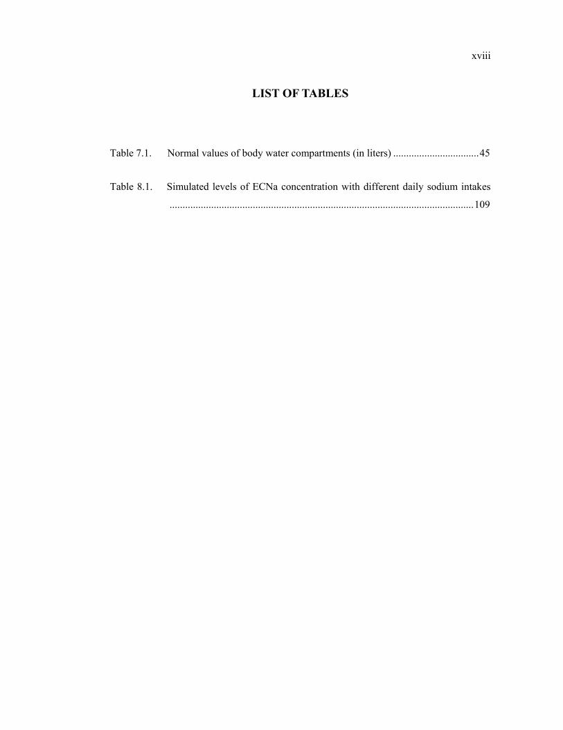
Table 7.1. Normal values of body water compartments (in liters) .................................45
Table 8.1. Simulated levels of ECNa concentration with different daily sodium intakes
.....................................................................................................................109
xix
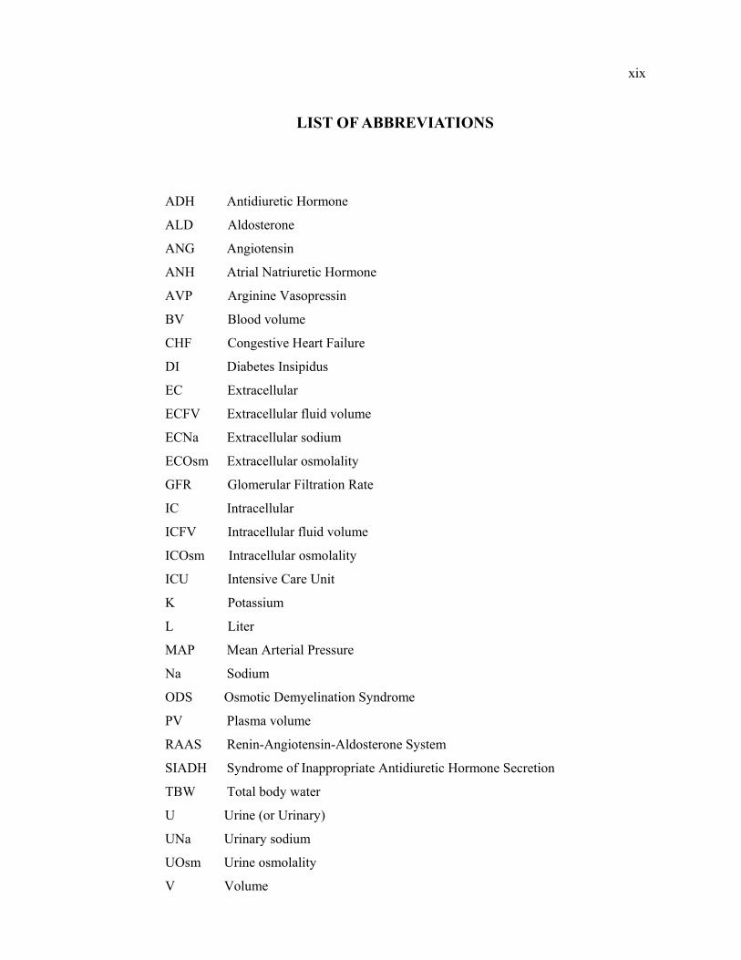
LIST OF ABBREVIATIONS
ADH Antidiuretic Hormone
ALD Aldosterone
ANG Angiotensin
ANH Atrial Natriuretic Hormone
AVP Arginine Vasopressin
BV Blood volume
CHF Congestive Heart Failure
DI Diabetes Insipidus
EC Extracellular
ECFV Extracellular fluid volume
ECNa Extracellular sodium
ECOsm Extracellular osmolality
GFR Glomerular Filtration Rate
IC Intracellular
ICFV Intracellular fluid volume
ICOsm Intracellular osmolality
ICU Intensive Care Unit
K Potassium
L Liter
MAP Mean Arterial Pressure
Na Sodium
ODS Osmotic Demyelination Syndrome
PV Plasma volume
RAAS Renin-Angiotensin-Aldosterone System
SIADH Syndrome of Inappropriate Antidiuretic Hormone Secretion
TBW Total body water
U Urine (or Urinary)
UNa Urinary sodium
UOsm Urine osmolality
V Volume
xx
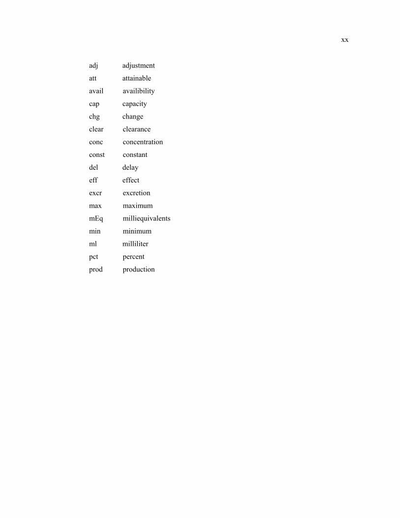
adj adjustment
att attainable
avail availibility
cap capacity
chg change
clear clearance
conc concentration
const constant
del delay
eff effect
excr excretion
max maximum
mEq milliequivalents
min minimum
ml milliliter
pct percent
prod production
1
1. INTRODUCTION
The homeostatic regulation of body fluids is important in almost every field of
medicine and has been thoroughly investigated in this century. The importance of the body
fluid system is based on its ability to keep a constant milieu interior, a condition of free
and independent existence, as emphasized by Claude Bernard (Schrier et al., 1993).
The task of the regulation of body water and its composition is mainly accomplished
by two control systems that are interacting in nature: the systems that control the body
water and the body sodium content, respectively. Like any other physiological control
system, these systems are governed by what is known as negative (compensating)
feedback. Body water essentially consists of extracellular (EC) and intracellular (IC) water.
The main system for body water regulation is the Antidiuretic Hormone (ADH) - thirst
feedback system. The basic function of ADH is to control the sodium concentration and
the body water volume. It accomplishes this by reacting to any variation in the
extracellular sodium concentration so as to restore it to its normal value. The regulation of
sodium balance is more intricate, and the main systems involved are the Aldosterone
(ALD) System, the Atrial Natriuretic Hormone (ANH), and the renal mechanisms. The
main function of ALD is to maintain a constant EC fluid volume. It achieves this by
reacting to changes in Angiotensin hormone levels, which is a function of blood pressure.
Similarly, ANH tries to maintain a constant EC fluid volume, and it also reacts to changes
in sodium content and tries to keep a constant sodium to potassium ratio. Sodium and
potassium are confined to the EC and to the IC fluid compartments, respectively.
Problems associated with body fluid disorders are very common in hospitalized
patients. Among these, water intoxication (or hyponatremia) defined as an abnormally low
level of plasma sodium concentration, is the most important body fluid disorder with the
potential for significant mortality. The treatment of hyponatremia constitutes a problem,
partly because all available therapies have significant limitations. For example diuretics, a
commonly used drug category for hyponatremia, are associated with many potential
2
complications such as significant urinary losses of electrolytes. Inappropriate doses of
drugs may also cause dehydration.
Furthermore, it is observed that a big portion of hyponatremia incidences are in fact
“hospital-acquired”. Most of these patients acquire hyponatremia as they receive
intravenous fluids, which is a very common practice in hospitals. Today, more than 75% of
currently recommended intravenous fluids are in the form of electrolyte-free water, which
is known to aggravate hyponatremia (Halperin and Bohn, 2002). Moreover, many cases are
associated with progress from mild to more severe levels of hyponatremia during
management of other disorders. This growing trend raised doubts related to hyponatremia,
and inspired many studies on its diagnosis and optimum therapy for reevaluation of the
current practices (Shafiee et al., 2003).
Due to the feedback complexity of the underlying structure and its interactions with
various pharmacological means, body water regulation and its disorders constitute a
suitable area for system dynamics simulation modeling. However, no closed-loop therapy
approach for disorders of hypo- and hypernatremia has been yet attempted (Northrop,
2000). This study attempts to build a closed-loop system dynamics model for body water
disorders, and particularly for ADH induced hyponatremia.
First, in the following section, main disorders of body fluid control systems are
discussed. Then, a brief review of systems-theoretic research in body water disorder
treatment is provided. In the remaining chapters we present our system dynamics model,
together with major validity tests results. Finally we convert the model into an interactive
simulation game and discuss the results obtained from some typical gaming experiments.
3
2. CLINICAL ABNORMALITIES OF BODY FLUID REGULATION
In health, total body water and its distribution throughout the body is maintained
between narrow limits. This task is accomplished by two distinct but interactive systems
that respectively regulate the extracellular fluid (ECF) volume/sodium content and the total
body water (TBW)/osmolality (The normal operation of these homeostatic systems is
explained in Section 7.1). Due to their functional interrelationships, any influence which
alters the balance of one of these systems inevitably affects the balance of the other.
Therefore, it is important to differentiate the clinical abnormalities of ECF volume/Na
content from those of the TBW/osmolality regulation.
2.1. Disturbances of Body Sodium Content
As the major cation of the EC fluid, the sodium content determines the ECF volume.
Therefore disorders of sodium metabolism are always manifested as disorders of volume
status. Moreover, due to the close interrelationship between ECF volume and the mean
arterial pressure (MAP), MAP is also dysregulated. Disorders of sodium metabolism
commonly coexist with disorders of water and fluid-electrolyte balance; thus a careful
clinical examination and laboratory tests help to the correct diagnosis and evaluation.
Disturbances in body sodium content can be broadly categorized into two groups:
2.1.1. Extracellular Fluid Volume Overload
These are abnormal conditions that are associated with expanded ECF volume and
generalized edema. Edema refers to a clinically detectable excess of extravascular ECF
volume, which may be localized or generalized. In patients with edematous states, the
effective arterial blood volume is reduced due to the maldistribution of ECF volume, which
in turn results in conserving sodium and water despite elevated body fluid volumes. The
4
prototypical disorders of this category are congestive heart failure (CHF), hepatic cirrhosis,
and nephrotic syndrome (Bagby et al., 1998).
2.1.2. Extracellular Fluid Volume Depletion
These disorders are associated with deficiency and depletion of sodium. Most of the
time, absent or diminished sodium intake is combined with excessive sodium loss, due to
vomiting, excessive sweat production or any other cause. Since loss of sodium leads to loss
of water so long as osmoregulation continues, ECF volume is also depleted. On the other
hand, the cell volume is unaffected from the loss of water, unlike in the case of the primary
loss of water. Hence, the burden of water loss is solely on the circulation. Another danger
is the possibility of a vicious cycle, which may develop due to activation of ADH-thirst
mechanism, and may result in retention of water without sodium.
2.2. Disturbances of Water Metabolism: Dysnatremias
Disorders of sodium and water metabolism are frequently encountered in
hospitalized patients. They are clinically manifested by disorders of EC sodium
concentration/dysnatremias, since the regulatory systems controlling water metabolism do
so by maintaining a constant EC sodium concentration. (The body water control
mechanism is explained in Section 7.1.1). Loss of water leads to hypernatremia, cell
shrinkage and widespread functional disturbances, particularly in the brain. On the other
hand, accumulation of water leads to hyponatremia, cell swelling and disturbances in
central nervous system. These disturbances are often coupled with other disturbances in
ECF volume, other electrolytes, and acid-base balance, and may present with a myriad of
symptoms which may mimic other disease states (Haslett et al., 2003)
In general, failure to maintain body water between narrow limits includes two
components. The first one is associated with the capability to dilute or concentrate urine
appropriately, and the second one is associated with the thirst function. The consequences
of a derangement in the urinary concentrating ability or thirst function vary widely, since
5
under normal conditions the human body has also some adaptive mechanisms for a
possible failure in one of these components. Furthermore, if one of these components fails
to function properly, the other component may still compensate this failure. However, in
most cases, disorders of urinary concentration and dilution are coupled with a concomitant
derangement of the thirst function, and this leads to marked changes in volume and
composition of body water (Jamison et al., 1982).
As mentioned before, clinical abnormalities of body water content can be categorized
according to the level of the EC fluid sodium concentration. Indeed, the EC sodium
concentration is the primary measurement of body fluid status. Under normal conditions,
the EC sodium concentration is maintained between 135-145 mEq/L, and 105-175 mEq/L
are the limits for survival.
2.2.1. Hypernatremia
Increased levels of EC sodium concentration may result either from loss of EC water,
or excess of sodium in the ECF. Ordinarily, the ADH-thirst mechanism ensures that a
primary loss of water only occurs when water intake is not possible (e.g. when water is in
short supply, or when the patient is very young, very old, unconscious or confused so that
he/she is unable to communicate). Therefore hypernatremia is mostly seen when there is
excess loss of water, e.g. with hyperventilation, high environmental temperature, fever, or
abnormal urinary loss (Haslett et al., 2003). The most common causes of hypernatremia
are indicated as inadequate hydration or correction (57%) and continuous diuretic
treatment (38%) (Halperin et al., 2002). In any case, when replenishment of excreted water
is inadequate, severe dehydration may cause weakness, fever, psychic disturbances,
hypotension, tachycardia, prostration, and death (Kasper et al., 2004). The clinical
situation of the patient becomes more aggravated as serum sodium concentration rises.
2.2.1.1. Diabetes Insipidus: Diabetes Insipidus (DI) is the most common type of pathologic
condition that is associated with hypernatremia. Insipidus means “tasteless”, therefore the
term “diabetes insipidus” distinguishes excessive urine flow (diabetes) caused by inability
6
to conserve water, from diabetes mellitus in which urine flow is enhanced due to excessive
glucose excretion. In DI, deficiencies of ADH production or action lead to production of
large amounts of dilute urine, which may reach up to 20-30 liters a day in severe cases.
More common, however, urine volume is moderately increased (2,5 to 6 L/day).
Consequently, the person becomes dehydrated and has to drink enough to replace this fluid
loss. The major causes of DI are pituitary or hypothalamic surgeries and severe head
injuries.
The failure to produce or secrete Antidiuretic Hormone (ADH) is called
hypothalamic DI (HDI). Most cases of HDI are mild, since at least 80% of ADH stores of
the body should be destructed before symptoms of polyuria (enhanced urine) and
polydipsia (enhanced drinking) may appear. If the thirst center of the patient is intact, the
person does not become overly dehydrated, and a mildly hypernatremic steady-state can be
reached at the expense of increased water turn-over. In moderate cases patients do not
complain if they become accustomed to excessive water turnover. However with severe
HDI, profound polyuria becomes a great inconvenience, since sleep and most activities of
the person will be continuously disturbed due to the need to void and drink. Water
deprivation could reduce the urine volume, but the ensuing thirst will be severe and if
water deprivation continues, severe dehydration and hypernatremia will develop. Today,
HDI can be successfully treated by using an ADH analogue in appropriate doses. However
there is considerable individual variation in the dose required, and higher doses may lead
to the other extreme, i.e. water intoxication/ hyponatremia. The second mechanism of DI is
a decreased ADH responsiveness of the kidney, termed nephrogenic DI (NDI). NDI may
have several reasons and its treatment is more difficult than the HDI.
2.2.1.2. Thirst Deficiency Syndromes: When thirst perception is impaired, ongoing fluid
losses may be uncorrected, and hypernatremia may occur even though ADH mechanism is
adequate to concentrate urine. In these cases, hypernatremia ensues as a result of chronic
inadequate intake of fluid, and in contrast to DI, water turnover is highly reduced. In
extreme cases, patients never experience thirst and if left themselves, they do not drink.
These disorders are referred to as hypodipsic or adipsic hypernatremia, and they present a
major management problem. If underlying cause cannot be treated, the only treatment
7
option is to give adequate fluid intake. Moreover, EC sodium concentration has to be
checked frequently in order to prevent extreme fluctuations in EC sodium concentration
that may cause crossings from hypernatremia to hyponatremia, and vice versa. This form
of hypernatremia is indeed life threatening, but also extremely uncommon.
2.2.2. Hyponatremia
Water intoxication or hyponatremia is the most common and potentially serious
electrolyte abnormality in hospitalized patients (Shafiee et al., 2003). It is defined as an EC
sodium concentration of less than 135 mEq/L. Decreased levels of EC sodium
concentration may result either from loss of EC sodium, or excess of water in the EC
compartment. The net result is always a dilution of body fluids. This affects the central
nervous system, and impairs mental processes. Cells expand due to extra water, and so
they put stress on the organs, especially on the brain, which has little room to expand.
2.2.2.1. Clinical Importance of Hyponatremia: The importance of ECNa concentration is
based on its effect on the intracellular (IC) compartment volume. The distribution of water
between the ECF and ICF is determined by the ECNa concentration, since the IC solute is
relatively constant and water crosses the cell membranes easily to equalize the IC and the
EC osmolalities. For example, if ECNa concentration rises, the ECF volume increases, and
the ICF volume decreases by the same amount. Therefore, the ICF volume is inversely
proportional to the ECNa concentration and the ECNa concentration is indeed used as an
indicator for ICF volume. Thus hyponatremia implies that the ICF volume is expanded.
This poses a threat particularly for the brain because brain is confined to a rigid space, the
skull and approximately 65% of total brain is IC water. Therefore it cannot gain
intracellular particles in an acute setting, and brain edema may develop easily, since an
increase in brain water of more than 5-10% is life threatening (Bray et al., 1989).
In contrast to the “acute” hyponatremia (developed in less than 48 hours), “chronic”
hyponatremia is much better tolerated by the brain cells. In fact, brain is the only
mammalian organ that is able to regulate its volume by adjusting its solute content. In
8
hypernatremia, the brain cells initially shrink, but gradually increase their solute content
over the next few hours and restore their normal volume. On the other hand, in
hyponatremia they first swell, but then they lose solute with water, and again restore their
volume.
3.2.2.2. Causes of Hyponatremia: The most common causes of hyponatremia are the
Syndrome of Inappropriate Antidiuretic Hormone Secretion (SIADH) (38%), incorrect
hydration (19%), and continuous diuretic treatment (30%) (Halperin and Bohn, 2002).
Clinical examination can reveal the underlying cause of hyponatremia, and the essential
tests include the ECNa concentration, the urine osmolality, and the urine sodium
concentration.
3.2.2.3. Symptoms of Hyponatremia: Hyponatremia is associated with a broad spectrum of
neurological symptoms related to both to the severity and rapidity of the change in the EC
sodium concentration. If these clinical signs are present, hyponatremia is called
“symptomatic”; otherwise it is termed as “asymptomatic” hyponatremia. When ECNa
concentration falls below 125 to 130 mEq/L, nausea and malaise may be seen as earliest
findings. Depending on the degree of water retention, the symptoms may expand to include
vomiting, headache, disorientation, lack of coordination, eventually followed by confusion
(water intoxication), convulsions, coma and respiratory arrest if the EC sodium
concentration falls below 115 to 120 mEq/L.
3.2.2.4. Frequency: Hyponatremia is usually observed in patients in hospital settings, and
incidences of hyponatremia depend largely on criteria used for diagnosis. It may rise up to
15-22%, when hyponatremia is simply defined as an ECNa concentration of less than 135
mEq/L; but only 3-5% of patients have an ECNa concentration of less than 130 mEq/L.
The clinical consequences of hyponatremia are rarely seen when it is greater than 125
mEq/L and are generally seen when it is less than 120 mEq/L (Verbalis, 1998).
Hyponatremia affects all races with equal gender distribution; however it is more common
in the elderly population.
9
3.2.2.5. Basic Types of Hyponatremia: As with the hypernatremia, hyponatremia can be
classified into three basic types depending on the EC volume status of the patient, i.e.
normovolemic (euvolemic-clinically normal ECF volume), hypervolemic, and
hypovolemic. That means it is possible to see hyponatremia with a decreased total body
water as well as with overexpansion of total body water. If hyponatremia results from loss
of sodium, it is called hypovolemic hyponatremia and is associated with decreased ECF
volume. The underlying reasons may be diuretic usage, vomiting, diarrhea, etc. On the
other hand, hypervolemic hyponatremia occurs in sodium retaining, edema forming states
such as liver cirrhosis, renal disease and congestive heart failure (CHF), which are
mentioned among the disorders of sodium metabolism in Section 2.1. Indeed, both
hypovolemic and hypervolemic hyponatremia are secondary complications of a primary
disturbance in ECF/sodium metabolism Therefore they especially tend to occur when the
primary ECF/sodium disorder is severe. In contrast, the disorders in the category of
euvolemic hyponatremia entail primary disturbances of body water osmolality/water
regulation, induced by inappropriate production of ADH or by other disturbances that
impair water excretion (Bagby, 1998).
Euvolemic hyponatremia is the most common type of hyponatremia of hospitalized
patients, which accounts for about 60% of all types of chronic hyponatremia, and the
syndrome of inappropriate antidiuretic hormone secretion (SIADH) is by far the most
frequently encountered cause of euvolemic hyponatremia (Hirshberg and Ben-Yahuda,
1997)
2.2.2.6. Syndrome of Inappropriate Antidiuretic Hormone Secretion (SIADH): SIADH was
first described in two patients with bronchogenic carcinoma in 1957 (Scwartz et al., 2001),
and then it is characterized by Bartter and Schwartz. The cardinal features of the SIADH
are as follows: Hyponatremia with low EC osmolality, urine osmolality greater than the EC
osmolality, excessive renal sodium excretion, absence of edema and volume depletion,
normal adrenal and renal function. This syndrome is caused by persistently elevated levels
of ADH when combined with sustained fluid intake.
10
Excessive secretion of ADH results in water retention and consequent dilution of
body fluids by forming decreased volumes of highly concentrated urine. Consequently, the
most commonly observed effect is a seriously reduced ECNa concentration. ECNa
concentration sometimes falls from its normal value of 142 mEq/L to as low as 110 to 120
mEq/L. At those values, patients may die due to coma and convulsions.
As mentioned before, in most patients with this syndrome ECF volume stays within
normal limits, and arterial pressure is not elevated. (Schwartz et al., 2001) This can be
explained as follows: The inappropriately retained water distributes evenly between the
ECF and ICF. The expansion of ECF activates the ECF volume/Na content control
system, and this promotes a transient Na loss (Kaye, 1966). Thus, the ECF volume reaches
a new steady-state within a clinically normal range, and most of the excess water is
confined to the IC compartment. In fact, a subtle ECF expansion may be present, however
assessment of the volume status is difficult when differentiating euvolemia from mild
forms of hyper-and hypovolemia (Bagby, 1998).
SIADH Differentials: Hyponatremia is often related to SIADH; nevertheless it can also be
associated with different clinical entities. These can be divided into two groups, according
to the impairment in water excretion. Diuretics, renal failure, decreased solute intake and
cerebral salt wasting are disorders in which renal water excretion is somehow impaired. On
the other hand, primary polydipsia and reset osmostat belong to the second group of
hyponatremic disorders with normal water excretion. It is important to differentiate SIADH
from these disorders before instituting a treatment strategy
(http://www.emedicine.com/med/topic3541.htm)
Hormone Levels in SIADH: As mentioned before, a marked and transient natriuresis
occurs at the beginning of the SIADH. This seems like an adaptive response of the body to
prevent a possible elevation of arterial pressure. There is also a discussion whether this
natriuresis aggravates hyponatremia (Vieweg and Godleski, 1988, Song et al., 2004). On
the other hand, Cogan et al. (1988) reported that hyponatremia is mainly related to water
retention, and not to sodium depletion. This Na excretion is attributed to the levels of
11
“volume” hormones; especially the levels of Aldosterone (ALD) and Atrial Natriuretic
Hormone (ANH).
It is also logical to assume that excessive Na losses resulting from this natriuresis
may secondarily activate the Na retention mechanisms of the body (Song et al., 2004).
Both of these Na excretion and Na retention mechanisms are associated with hormone
levels of ALD and ANH.
It is observed that in SIADH, plasma ANH levels are increased while plasma ALD
levels are decreased. It is concluded that ANH may be partly responsible for the natriuresis
in SIADH, since the urinary sodium excretion rate is found to be significantly correlated
with the levels of ANH (Cogan et al., 1988). Some studies indicate that ANH levels return
to their normal values after the natriuresis; however some relate ANH levels to the degree
of hyponatremia and find a negative correlation between ANH and the ECNa levels. On
the other hand, ALD levels are mostly reported to fall, contrasting with the state of sodium
depletion (Cogan et al., 1988). However it is also observed that severe hyponatremia is
associated with a delayed rise in ALD levels.
The conflicting reports regarding to the level of ALD in SIADH shows that the
relation between hyponatremia and ALD secretion is not well recognized. One of the
reasons may be the delay between the rise in ALD levels and the onset of hyponatremia.
This may result from the fact that the stimuli for ALD secretion actually compete in
SIADH (Song et al., 2004). While volume expansion promotes a fall in ALD release,
decreasing levels of ECNa concentration dictates a rise in ALD. Therefore it should not be
surprising that excessive Na losses in SIADH secondarily activate the Na retention
mechanisms of the body, like the delayed increase of ALD hormone.
Adaptive Mechanisms in SIADH: Disturbances of every physiological control system in
the body, as well as disturbances in water and electrolyte balance, are rapidly followed by
adaptation. The adaptive responses of the body do not restore the body to its normal, but
12
still prevent further detrimental changes and help to maintain a new-steady-state condition
(Cumming and Plant, 2003).
In SIADH, the transient natriuresis helps to maintain the ECF within normal limits;
however this adaptation response does not stop the accumulation of excess water in the
body. In order to achieve a steady-state condition, both the water and the salt balance
should reach equilibrium. There are two possibilities to stop the accumulation of excess
water. First one is to restrict the fluid intake on purpose, and the second one is to increase
the urine flow until the intake and output of water are equal. As mentioned before, SIADH
patients continue to drink for unknown reasons. Therefore the only possibility that may
prevent a possible circulatory collapse due to overexpansion of body water would be a
mechanism that increases urine flow by reducing the urine concentration. Indeed, that is
the case observed in severe SIADH patients and it is called “ADH-escape” phenomenon,
or “escape from ADH-induced antidiuresis”, which limits the amount of water retained in
the body by reducing the antidiuretic effect of the circulating ADH, and re-establishes the
body water balance. The result is a newer and stable, albeit lower, sodium concentration,
and higher body water content (Verbalis et al., 1989; Ecelbarger et al., 1998; Song et al.,
2004; Ishikawa et al., 2004; Verbalis; 1994, 1998;
http://www.emedicine.com/med/topic3541.htm).
2.2.2.7. Management of Hyponatremia: The diagnosis and management of salt and water
abnormalities in general and hyponatremia in critical patients in particular is also often
challenging since inappropriate treatment can aggravate the problem. These challenges are
especially important for problems of fluid and electrolyte balance in an Intensive Care Unit
(ICU) setting because they may become life threatening very rapidly. The most important
aspects that should be paid special attention for clinical evaluation of hyponatremia are the
EC fluid volume status of the patient, the symptoms and signs present, the rate at which
hyponatremia has developed, and the severity of the hyponatremia. (Cumming and Plant,
2003).
In general, clinical features and symptoms of hyponatremia are rarely seen with an
ECNa conc. of more than 125 mEq/L and these patients may not require specific treatment
13
to raise their ECNa conc. However with more severe degrees of hyponatremia, i.e., at
values below 110 mEq/L, hyponatremia may produce significant morbidity and mortality
because of coma and convulsions (Verbalis, 1998). Therefore, an ECNa conc. of 110
mEq/L or less is thought to be extremely dangerous in general, and urgent assessment and
some form of therapy is required. At levels below 110 mEq/L, mortality rates of 33% to
86% have been cited, though some researchers have smaller estimates (Sterns, 1987).
The rate at which hyponatremia is developed is another differentiating factor for the
treatment strategy as mentioned above. In fact the first decision one must take when
dealing hyponatremia is to determine whether it represents an acute (documented course is
less than 48 hours) or a chronic condition (Halperin and Bohn, 2002). It is crucial to
separate acute from chronic hyponatremia before starting treatment, since the dangers for
the patient are different (Edoute et. al., 2003). The main risk with acute hyponatremia is
brain cell swelling, and hence the treatment of acute hyponatremia should focus on
reducing the size of the brain. Even the mild symptoms of an acute hyponatremia may lead
to clinical deterioration very rapidly so the treatment must be prompt and vigorous. In
contrast, the main risk with chronic hyponatremia is the osmotic demyelination syndrome
(ODS, also known as central pontine myelinosis), which may appear secondary to an
overly aggressive therapy and produce neurological morbidity and mortality in some cases
(Halperin and Bohn, 2002; Song, 2004). Indeed, rapid correction of hyponatremia due to
any cause can produce serious irreversible neurological consequences, ODS, and death.
The fact that an overly rapid correction of hyponatremia may cause brain damage
caused an ongoing controversy regarding to optimal treatment guidelines of severe
hyponatremia. Physicians and researchers have been reviewed the subject extensively with
the intention for finding the most appropriate therapy for this important group of patients
(Baylis, 2003); but to date, all of the present therapies in patients with ADH-induced
hyponatremia have significant limitations (Janicic and Verbalis, 2003) The debate is also
extending over the degree and time of onset of hyponatremia, the development of clinical
measures and long-term morbidity and mortality.
14
On the other hand a general consensus has emerged that is directed towards
balancing the risks of hyponatremia against the risks of its correction, although both risks
vary greatly between individuals. According to this consensus based on clinical and
experimental results, the rate of correction of symptomatic hyponatremia should be no
more than 0,5 mEq/L per hour, and the initial treatment should be stopped once a mildly
hyponatremic range of ECNa conc. has been reached (apprx. 125 to 130 mEq/L) (Verbalis,
1998). According to the most recent literature, acute hyponatremia should be treated
promptly with hypertonic saline (3%) in order to prevent seizures and respiratory arrest.
On the other hand, for patients with chronic symptomatic hyponatremia, correction must be
rapid during the first few hours (to decrease brain edema), but the total correction should
not exceed 8-12 mEq/L over 24 hours to avoid the development of ODS (Decaux, 2001).
ODS is dangerous since demyelination of pontine and extrapontine neurons lead to
quadriplegia, pseudobulbar palsy, seizures, coma, or death. Therefore, frequent
measurements of ECNa concentration during the correction phase are essential to avoid
overcorrection. Ideally, the patient should be monitored in an ICU setting.
However in all instances, successful treatment depends on a correct diagnosis of the
underlying problem, i.e., finding the condition that caused hyponatremia and include it in
the clinical analysis and not simply treat an ECNa conc. value, since various
pathophysiologic mechanisms can be at the origin of hyponatremia.
Presently, physicians have two main alternatives when treating hyponatremia: a)
They can try to limit fluid intake, and/or b) they can reduce ADH or its effect in the
kidney.
Water Restriction: When the underlying cause of the SIADH cannot be treated, water
restriction is the present mainstay of treatment as the most traditional mode of therapy. To
be more explicit, water restriction means to restrict total fluid intake to less than the total
output; since in SIADH, nonosmotic secretion of ADH results in overexpansion of body
fluids only if water intake exceeds the sum of insensible and urinary output. In fact, in a
patient with a normal-functioning thirst center no consequences may be seen; however in
another patient who is unable to communicate or whose thirst center is not appropriately
15
functioning, catastrophic results may appear. Infants and elderly patients constitute the
most risky group in terms of the possible consequences, since they are less able to indicate
their thirst, or have deficiencies in their thirst response (Hirshberg and Ben-Yehuda, 1997).
Therefore it is important to note that excess ADH secretion alone is not sufficient to
produce hyponatremia, and both thirst and the ADH system have to be dysregulated to
create the hypoosmolality. Indeed it was shown in hyponatremic patients that they cannot
suppress their fluid intake, and they even have an elevated daily fluid intake which was
found to be in the order of 2.0-2.5 l. (Palm et al., 2001). In other words, hyponatremic
patients have a dysregulated thirst function in addition to inappropriate ADH release,
which often results from an associated defect in the osmoregulation of thirst.
Though water restriction seems to be the simplest solution to the problem,
compliance with it is poor, in part because ADH also stimulates thirst, and because in the
long term it can be difficult and unpleasant/distressing for the physician and for the patient.
Moreover, severe water restriction could only be imposed while the patient is hospitalized,
but once the fluid intake is liberalized or even relaxed, hyponatremia will recur. Therefore
successful treatment comprises liberalization or at least relaxation of fluid restriction.
Some combination of drug/ fluid therapy is advocated to manage chronic hyponatremia in
addition to a mild fluid restriction that could be sustained by the patient.
Today there are two main categories of drugs which may be used for reducing the
effect of ADH in the kidney, diuretics and ADH-Antagonists:
Diuretics: Diuretics are occasionally used in the management of edematous (volume
loaded) hyponatremic states and chronic SIADH, if urine is highly concentrated (Janicic
and Verbalis, 2003; Goh, 2004). The category of loop diuretics is mainly known for
reducing the ability to excrete dilute urine (Nyugen and Kurtz, 2003). The net effect of
loop diuretics on urinary concentrating ability is to prevent formation of either
concentrated or dilute urine (Jamison, 1982).
16
However diuretics are also associated with some potential complications. They cause
significant urinary losses of sodium, potassium, and magnesium and thus may cause an
electrolyte imbalance such as hyponatremia and hypokalemia. Indeed, the group of
thiazide diuretics is well-known for inducing severe hyponatremia. They were responsible
for inducing severe hyponatremia in 94 percent of 129 cases reported between 1962 and
1990; unlike furosemide, the most common loop diuretic. (Sonnenblick, 1993). Diuretics
also activate the renin-angiotensin-aldosterone system (Weir and Dzau, 1999). In spite of
these counterindications, in SIADH, they still constitute an alternative treatment approach
when combined with plentiful sodium intake.
ADH-Antagonists (“Aquaretics” or “water diuretics”): These constitute the most recent
and promising pharmacological tool for the therapy of disorders of water metabolism, and
specifically for the treatment of patients with water excess and consequent dilutional
hyponatremia (Schrier et al., 1993; Janicic and Verbalis, 1993). They have been also
termed as “aquaretics” or “water diuretics” because of their ability to increase free water
excretion without affecting solute excretion. Orally effective ADH receptor antagonists
were reported in 1991 and 1992 (Yamamura et al., 1991 and 1992), and this has aroused a
great interest in ADH research and clinical use. Saito et al. (1996) were the first to report
results of a clinical trial in hyponatremic SIADH. They demonstrated that ADH
Antagonists induce prompt and dose-dependent increases in urine volume and parallel
decreases in urine osmolality; and consequently a substantial improvement in ECNa
concentration is observed. The ongoing ADH research now focuses on the development of
a potent ADH-receptor antagonist that can be safely administered orally over the long
term.
Possible side–effects of ADH receptor antagonists are also indicated. At high doses,
these drugs appear to increase the current ADH concentration in plasma (Wong and
Verbalis, 2002). Moreover, high doses may also dispose the patient to dehydration, or even
to ODS, if correction is rapid. Therefore, patients with SIADH receiving ADH-Antagonists
require close monitoring to prevent a rapid correction. It should also be kept in mind that
ADH-Antagonists should only be used in euvolemic (blood volume is normal) or
hypervolemic (blood volume is elevated) disorders, e.g., in SIADH, cirrhotic heart failure,
17
cirrhosis with ascites. It is obvious that ADH-Antagonists are not an appropriate choice of
drug for hypovolemic hyponatremia since it will aggravate hypovolemia and may lead to
dehydration and hypotension due to an increased free water excretion. However, when
taken together, ADH-Antagonists appear to be effective in correcting hyponatremic
disorders and promise to become the most popular therapeutic agents in that area.
Fluid Therapy: Fluid therapy (also known as intravenous fluid administration or saline
infusion) is a quite ordinary therapeutic means for hospitalized patients and more than 75%
of the currently recommended saline is given in the form of electrolyte-free water (0.2 %
saline). The five most common reasons to infuse intravenous fluids are (Shafiee et al.,
2003): Defending normal blood pressure, returning the ICF to normal, replacing ongoing
renal losses, giving maintenance fluids to match insensible losses, and the need for glucose
as a fuel for the brain.
However there are still many problems associated with intravenous fluid
administration e.g., finding the optimum therapy for a body fluid disturbance is a very
important but yet unsolved question. Recently it became clear that traditional
recommendations for intravenous therapy have to be reevaluated, partly because it is seen
that patients who have received intravenous fluids often develop hyponatremia hospital
(Shafiee et al., 2003). This and other problems regarding saline administration led
physicians to extensively review the subject from various viewpoints.
The three most commonly used categories of intravenous fluids, which are also
included in the model, are hypertonic, isotonic, and hypotonic fluids, which are classified
according to their sodium content. Their description and implications for hyponatremia
management can be summarized as follows:
a) Isotonic Saline: This solution has an [Na+] concentration similar to that of the
normal plasma, i.e., it is 0.9 % saline (154 mEq/L Na). Isotonic saline solutions have been
also termed as “Replacement solutions”, or “Normal Saline”. They are used to replace the
EC fluid, because the fact that their [Na+] is similar to that of the EC fluid effectively
18
limits their distribution to the EC fluid. The infusate distributes between the interstitial
fluid and the plasma in proportion to their volumes, and the IC fluid volume does not
change. As a result, isotonic saline should be considered where the patient is volume
depleted.
b) Hypotonic Saline: Hypotonic solutions vary between 0.45% and 0.18 % saline (77
and 30 mEq/L Na). They have an osmolality smaller than the normal plasma osmolality. In
general, they are considered less dangerous in fluid therapy, but that can be a grave error in
some cases.
Today, more than 75% of the currently recommended saline is given in the form of
electrolyte-free water (0.2 % saline) in hospital settings, since traditional recommendations
require that hypotonic saline be infused to the patient as a maintenance fluid. However it is
obvious that electrolyte-free water will accumulate in the body when ADH is acting.
Moreover, frequently it is seen that patients arrive hospitals with a low ECNa conc.
because they drank electrolyte-free water while ADH is released secondary to their illness.
It would be a grave error to give these patients extra electrolyte-free water in the form of a
hypotonic solution. As a consequence of these, physicians should not use hypotonic
solutions if the ECNa concentration is lower than 138 mEq/L, unless if they want to limit
the rise in ECNa concentration due to a rapid diuresis.
It should also be kept in mind that some other factors exist which increases the risk
of developing a more severe hyponatremia if hypotonic solutions are administered. These
are the age of the patient, and the skeletal muscle mass relative to body weight. Brain cell
number decreases with age, and this puts children and young adults at greater risk. The
second factor is also important because 50% of body water is in skeletal muscle in normal
subjects (Shafiee et al., 2003).
c) Hypertonic Saline: Hypertonic saline 3% has an osmolality (about 900 mEq/L)
three times that of plasma. Its sodium content limits its distribution to the EC fluid, very
much like an isotonic saline solution. However in addition to that, a hypertonic solution
19
will also draw water out of cells and thereby decreases the IC fluid volume, unlike the
isotonic saline.
Current standard therapy for severe hyponatremia is administration of graded
amounts of hypertonic (3%) saline. However there is a general consensus stating that
hypertonic saline should be infused very slowly and carefully in chronic hyponatremia of
SIADH, and should be reserved for either significantly symptomatic patients or those with
symptomatic acute hyponatremia of duration more than 3 days (Saito et al., 1996).
Moreover, it is generally recommended that saline infusion should stop when the ECNa
concentration reaches 120-125 mEq/L. After this value is attained, other more traditional
modes, e.g. fluid restriction, are recommended (Nyugen and Kurtz, 2003).
20
3. DYNAMIC MODELING OF PHYSIOLOGICAL SYSTEMS
3.1. Systems Theory in Physiological Models
The capability of living beings to maintain their constancy has aroused a great interest
for long time. Hippocrates held the idea that disease is cured by natural powers, which will
later be reformulated as: “Each disturbing influence induces by itself the calling forth of
compensatory activity to neutralize or repair the disturbance” by Pflüger (Cannon, 1932).
However the corresponding term of “homeostasis” was first used by Walter Cannon, a
professor of physiology, in his book The Wisdom of the Body (1932). In this book, Cannon
described the working principles of many physiological systems like the control of blood
pressure, blood sugar, water intake, and salinity. These systems appeared to be very
different in their design and composition, but Cannon saw that they obey the same
principles when viewed in terms of homeostasis, and suggested that physiological systems
are mainly dominated by negative feedback loops.
Although Cannon made use of the concepts of today’s dynamic systems, he only
used qualitative descriptions in his writings. The second pioneer of systems thinking in
physiology, namely Arthur Guyton, was the first to introduce the concept of systems
analysis to physicians. From 1950’s on to the end of century, he has built mathematical
physiology models combining the results of extensive experimentation with the tools of
mathematics, physics, engineering and physiology. He built models of circulatory body
fluid dynamics mainly to examine the reasons of hypertension; but the most important
message of his works was that complex system behaviors can be examined quantitatively,
and in terms of grossly lumped system parameters. This approach then led to the
emergence of biomedical engineering, a discipline which changed physiology into a much
more quantitative science.
In recent years there has been a considerable increase in the application of the
methods of mathematical modeling and dynamic systems analysis, both in physiology and
clinical decision making. It is also recognized that the required systems approach is
21
interdisciplinary, and thus it requires collaboration of clinicians, physicians,
mathematicians, biologists, and other related life sciences. Application of systems
approach to physiology can both provide a greater understanding of the nature and
behavior of complex physiological processes, and can also be used as an aid in the
diagnosis and treatment of a disease. The increasing trend for universal health care and the
subsequent shift in medicine from individual practice to health care systems is another
reason that promotes the current trend in physiology. (The financial cost of US health care
systems is currently 8% of GNP, and it continues to increase at about 12% per year
(Carson et al., 1983).
3.2. Models for Fluid-Electrolyte Dynamics
The system for regulation of body fluid volume (also called the water balance
system) is important to understand diseases such as hypertension and dysnatremias.
Though it seems a simple one, this system is one of the most complex physiological
systems in the body since it involves many other subsystems. Over the last 50 years
numerous models have been presented to illustrate the complexity of body fluid regulation
with its interrelationships to the renal, respiratory, endocrine, and cardiovascular systems.
However another big portion of fluid-electrolyte models only attempt at modeling the parts
of kidney function in isolation, and do not consider the interactions of kidney with the rest
of the body. These will not be mentioned here.
First models that represent certain aspects of renal control of body fluids belong to
DeHaven and Shapiro (1967) and Reeve and Kulhanek (1967). Whereas DeHaven and
Shapiro (1967) only focused on the excretion mechanisms of the body, Reeve and
Kulhanek (1967) also included a water-drinking mechanism which they believed to be at
least equally important as the excretion mechanism in controlling body fluid volumes.
First integrated models of body fluid regulation that also consider the circulatory
system include those by Ikeda (1979) and Abbrecht (1980). The model of Ikeda and co-
workers is an integrated model of fluid-electrolyte and acid-base representation. However
22
the most complex analysis of body fluid dynamics belongs to Guyton and co-workers,
which is first published in the Annual Review of Physiology in 1972. In his analysis,
Guyton reviewed all aspects of circulatory dynamics, as well as the dynamics of the free
fluids in the tissues, the fluid in the tissue gel, the fluid in the cells, renal excretion of fluid,
and endocrine control of body fluid volumes. Moreover, Guyton constructed an overall
circulatory model for examining the causes of hypertension, and Guyton and Coleman
(1967) proposed both a simple and a complex model for the long term regulation of
circulation. This model has inspired many other studies in this field, but it is also criticized
due to its gigantic size and some limitations (Sagawa and Kiichi, 1975).
Cameron (1977) developed a simplified version of Guyton et al. (1972), and adopted
the approach of Ikeda and co-workers. On the other hand, Uttamsingh (1981) and Badke
(1972) used the simple model of Guyton (1967). Uttamsingh (1985) has also extended his
model for the clinical application of patients with renal failure who need regular
hemodialysis. A large number of other renal models can be found in Flood et al. (1984a).
Recently, a long-term cardiovascular system model is developed by Karaaslan (2004) that
integrates the previous models developed by Guyton, Uttamsingh and Coleman. This study
focuses on the long-term analysis of the effect of renal symphatetic nerve activity on
arterial pressure and sodium excretion.
In this study we adopt a system dynamics modeling approach to model the body
water-electrolyte dynamics. The modeling methodology is discussed in Section 5.
23
4. PROBLEM DESCRIPTION AND RESEARCH OBJECTIVE
Disorders of sodium and water metabolism are frequently encountered in
hospitalized patients. Among these, hyponatremia is the most common and potentially
serious clinical disorder. Although most cases are mild, hyponatremia is clinically
important, and its diagnosis and subsequent management constitutes a challenging problem
for physicians. Hyponatremia is associated with increased levels of intracellular water
caused by osmosis to balance low levels of extracellular Na concentration.
The main risk with acute severe hyponatremia is brain swelling, a disorder which
may produce substantial morbidity and mortality in a very short time. Thus it requires a
very prompt and vigorous treatment. On the other hand, rapid correction of any type of
hyponatremia can lead to severe neurologic deficits and death, irrespective of the mode of
therapy. This dictates a careful treatment strategy which should balance the risks of
hyponatremia against the risks of its correction.
Treatment of hyponatremia involves drug therapy and/or intravenous fluid
administration. However treatment is often complicated. For instance, diuretics, a common
medication means, actually aggravate hyponatremia if inappropriately used. Similarly,
improper fluid administration is also known to complicate hyponatremia.
To sum up, both the diagnosis and management of body fluid disorders, in particular
hyponatremia, are challenging for physicians, in part due to the complex nature of the body
fluid system. It is foreseen that mathematical models of physiological systems can make a
significant contribution to the clinical diagnosis and to teaching of many aspects of
physiology. They can also provide a means for evaluating hypotheses concerning the
underlying pathology of a critical clinical disorder. This view has culminated in the growth
of simulation models that are employed as a tool for the therapy of clinical disorders, as
well as fluid-electrolyte disorders. Especially interactive simulation games are gaining
24
popularity as an interdisciplinary bridge between physicians, students, and other disciplines
that attempt to formalize physiological relations.
As a result, the goal of this study is to develop an interactive simulation model for a
particular body fluid disorder, i.e. hyponatremia, based on system dynamics methodology.
The first step towards this objective is to develop a well-validated system dynamics model
which represents the structure of the body water and sodium balance for an individual
normal adult subject with a given set of initial conditions. Then this model will be
modified and extended to include the effects of disease processes, related therapeutic
interventions, and possible necessary measurements for diagnosis. Finally, a game version
of the modified model will be produced which will allow the user to test the possible
effects of a given a set of treatment options on a virtual patient.
25
5. RESEARCH METHODOLOGY
The purpose of this modeling study is to represent dynamics of the body water and
sodium balance in normal and diseased states, with particular emphasis on the
physiological feedback mechanisms. It is known that the constancy of the body fluid
balance is maintained by various physiological control systems which employ negative
feedback, and many disease states are simply abnormalities of a particular control system.
However, the time delays and the interplay of various factors (physical, hormonal, etc.)
which regulate the function of the kidney makes it difficult or impossible to make
quantitative predictions without a mathematical model or computer simulation.
Considering the non-linear feedback structure of the system under concern, system
dynamics approach turns out to be very appropriate for the quantitative analysis of
problems concerning body fluid disturbances and therapy.
System dynamics methodology performs satisfactorily in analyzing and modeling
complex, large scale, non-linear dynamic systems, and particularly focuses on the inherent
feedback structure. The main assumption of system dynamics approach is that any system
is a whole and is composed of many sub-systems. Other important assumptions of System
Dynamics are direct causal relationships between variables and interdependence of causal
factors through feedback loops. The simulation-based experimentation procedure of system
dynamics gives insight about the dynamic complexity of the system under concern; helps
to identify the possible causes of the inherent problem, and to assess the overall effect of a
therapeutic intervention. This is an important advantage of the methodology over other
quantitative approaches considering the purpose of this study.
System dynamics methodology focuses on predicting the dynamic patterns that
would result from adopting a given set of policies, rather than predicting values of the
system variables point by point. This aspect makes system dynamics applicable to the
assessment and control of physiological systems, as any analysis of physiological control
system depends upon a broad understanding of the whole physiology, and an anticipation
of the overall system response to a series of interventions.
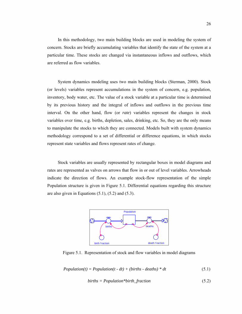
26
In this methodology, two main building blocks are used in modeling the system of
concern. Stocks are briefly accumulating variables that identify the state of the system at a
particular time. These stocks are changed via instantaneous inflows and outflows, which
are referred as flow variables.
System dynamics modeling uses two main building blocks (Sterman, 2000). Stock
(or levels) variables represent accumulations in the system of concern, e.g. population,
inventory, body water, etc. The value of a stock variable at a particular time is determined
by its previous history and the integral of inflows and outflows in the previous time
interval. On the other hand, flow (or rate) variables represent the changes in stock
variables over time, e.g. births, depletion, sales, drinking, etc. So, they are the only means
to manipulate the stocks to which they are connected. Models built with system dynamics
methodology correspond to a set of differential or difference equations, in which stocks
represent state variables and flows represent rates of change.
Stock variables are usually represented by rectangular boxes in model diagrams and
rates are represented as valves on arrows that flow in or out of level variables. Arrowheads
indicate the direction of flows. An example stock-flow representation of the simple
Population structure is given in Figure 5.1. Differential equations regarding this structure
are also given in Equations (5.1), (5.2) and (5.3).
Population
births deaths
birth f raction death f raction
Figure 5.1. Representation of stock and flow variables in model diagrams
Population(t) = Population(t - dt) + (births - deaths) * dt (5.1)
births = Population*birth_fraction (5.2)
27
deaths = Population*death_fraction (5.3)
The level of this system is Population. Population is increased from its current value
by the births flow and is decreased by the deaths flow. Remaining variables birth fraction
and death fraction are called converter (or auxiliary) variables and they represent how a
certain variable depends on another variable at a particular time. Finally, the connecting
arrows indicate a causal relationship between two variables in the system.
System dynamics methodology is composed of an iterative modeling process of five
stages and a subsequent experimentation (Sterman, 2000). The first stage is problem
articulation, which comprises the identification of the dynamic problem that needs to be
understood and solved. In this step, the system boundary and the time horizon of the study
are determined with selected key variables.
In the second stage of the methodology, a dynamic hypothesis is developed regarding
the dynamic problem of the system. This requires revealing the causal structure of the
system that involves the feedback relationships between system variables with respect to
the past behavior of the system.
The third stage consists of building the mathematical simulation model based on the
first two steps. Building of the stock-flow structure of the model is then followed by
estimation of parameters, equations and initial conditions based on the observed past data
and system behavior.
The fourth stage of the methodology is testing the validity of the simulation model
with respect to the problem of concern. This process is actually performed during the
development of the model, and includes both the validation of the model structure and its
behavior. First, the validity of the model structure is tested against the real system
relations. Only if the model passes this test, behavioral validation is performed by
comparing the output of the model with observed real dynamic behavior. In validity
28
testing, it is important that the model is reasonable under extreme conditions and the model
behavior is robust to uncertainties in initial conditions and parameters (Barlas, 1996).
The final stage of the methodology is to conduct experiments with the validated
model for the purpose of policy analysis and design. This experimentation stage includes
the study of the system behavior under various policies, scenarios and conditions. The
results are expected to provide insightful information for policy evaluation and design.
.
29
6. OVERVIEW OF THE MODEL
The purpose of this modeling study is to develop a dynamic representation of our
body fluid balance in normal and diseased states. For this purpose, the study is divided into
three parts. In the first part, the normal physiology of the body water balance and its
stability will be clarified, and in the second part, the dynamics of a specific body water
disorder, i.e. water intoxication/hyponatremia, will be investigated. Lastly, the modified
model of the second part will be used in an interactive simulation game for exploring the
possible effects of therapeutic interventions, and finding a successful therapy.
In health, total body water and body sodium content are tightly controlled by
maintaining a balance between intake of water and electrolytes from the gastrointestinal
tract and output of these as urine. In addition to that, not only the volume of the total body
water, but also its distribution between compartments, e.g. the blood volume is monitored
and maintained within close limits. This stable behavior can be observed in other
physiological control systems as well, and is termed as the “homeostasis” principle.
The mechanism for the regulation of water balance is often referred to as the ‘thirst-
ADH mechanism’. This system regulates water intake by controlling the perception of
thirst, and water output by ADH, which is responsible for urinary concentration and
dilution. The two most important factors that are monitored by this mechanism are EC
osmolality and intravascular volume (blood volume). The set point of both factors is
determined by hypothalamus, and therefore they are assumed to be exogenous to our
problem.
Figure 6.1 provides a brief causal-loop diagram of the overall model. The 1st and the
2nd loops demonstrate the ADH-thirst feedback mechanism for EC osmolality and total
body water control. Increasing EC osmolality increases the level of ADH, and as a
consequence of increased urinary concentration, water excreted in urine decreases. At the
same time, thirst perception is stimulated and water intake is increased.
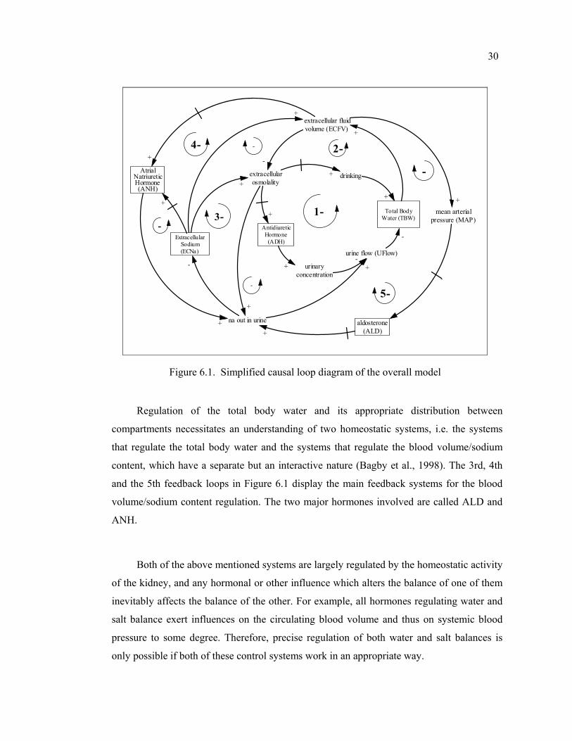
30
Total BodyWater (TBW)
extracellular fluidvolume (ECFV) +
urine flow (UFlow)
na out in urine
ExtracellularSodium(ECNa)
extracellularosmolality
-
-
AntidiureticHormone(ADH)
+
AtrialNatriureticHormone(ANH)
1- -
+
urinaryconcentration
drinking
+
2-
+
+
3-
-
-
+
mean arterialpressure (MAP)
aldosterone(ALD)+
5-
-
-
4-
-
+
-
+
++
+
+
Figure 6.1. Simplified causal loop diagram of the overall model
Regulation of the total body water and its appropriate distribution between
compartments necessitates an understanding of two homeostatic systems, i.e. the systems
that regulate the total body water and the systems that regulate the blood volume/sodium
content, which have a separate but an interactive nature (Bagby et al., 1998). The 3rd, 4th
and the 5th feedback loops in Figure 6.1 display the main feedback systems for the blood
volume/sodium content regulation. The two major hormones involved are called ALD and
ANH.
Both of the above mentioned systems are largely regulated by the homeostatic activity
of the kidney, and any hormonal or other influence which alters the balance of one of them
inevitably affects the balance of the other. For example, all hormones regulating water and
salt balance exert influences on the circulating blood volume and thus on systemic blood
pressure to some degree. Therefore, precise regulation of both water and salt balances is
only possible if both of these control systems work in an appropriate way.
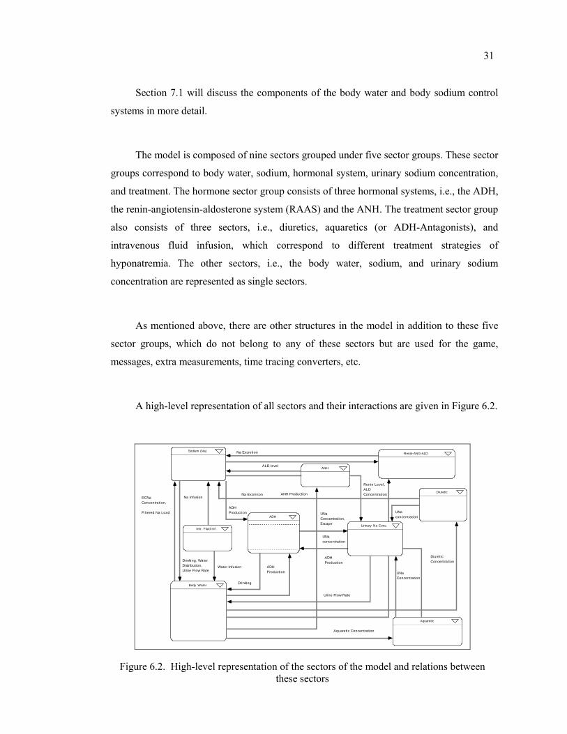
31
Section 7.1 will discuss the components of the body water and body sodium control
systems in more detail.
The model is composed of nine sectors grouped under five sector groups. These sector
groups correspond to body water, sodium, hormonal system, urinary sodium concentration,
and treatment. The hormone sector group consists of three hormonal systems, i.e., the ADH,
the renin-angiotensin-aldosterone system (RAAS) and the ANH. The treatment sector group
also consists of three sectors, i.e., diuretics, aquaretics (or ADH-Antagonists), and
intravenous fluid infusion, which correspond to different treatment strategies of
hyponatremia. The other sectors, i.e., the body water, sodium, and urinary sodium
concentration are represented as single sectors.
As mentioned above, there are other structures in the model in addition to these five
sector groups, which do not belong to any of these sectors but are used for the game,
messages, extra measurements, time tracing converters, etc.
A high-level representation of all sectors and their interactions are given in Figure 6.2.
ANH
Sodium (Na)
ADH
Aquaretic
Urinary Na Conc.
Body Water
Renin-ANG-ALD
Diuretic
Intr. Fluid Inf .
Drinking
ADH Production
Drinking, Water Distribution,Urine Flow Rate
ECNa Concentration,
Fi ltered Na Load
Na Excretion
ALD level
Renin Level, ALD Concentration
UNa concentration
Diuretic Concentration
Aquaretic Concentration
Urine Flow Rate
ANH Production
ADH Production
ADH Production
Na Infusion
Water Infusion
UNa Concentration
Na Excretion
UNa Concentration, Escape
UNa concentration
Figure 6.2. High-level representation of the sectors of the model and relations between these sectors
32
In the following sections, general overviews of the sector groups and the main
interactions with other sectors are presented. Underlying assumptions, the approach used,
and the structural details of sectors will be discussed throughout Chapter 7.
6.1. Body Water Sector
This sector is constructed to simulate the dynamics of total body water and its
distribution between body compartments. The major division of body water is into ECF and
ICF based on which side of the cell membrane the fluid lies.
The body water sector considers drinking as the only source of fluid intake. Both
continuous and discontinuous drinking options are modeled to simulate the drinking
behavior. Discontinuous drinking of the model represents a switch-on and switch off
structure, which only acts under some threshold body water level.
A fairly constant water loss, which represents the continuous escape in the form of
evaporation, and a varying urinary loss represent the two sources of loss of water from the
body. The urine flow rate and the drinking rate are the most important flows of the body
water sector which are determined by the feedbacks from other sectors, mainly the ADH,
urinary sodium (UNa) concentration, and the sodium (Na) sectors.
Details of this sector are discussed in Section 7.2.
6.2. Sodium Sector
The Na sector simulates the dynamics of Na+ of the EC fluid, since total body Na+ is
restricted mostly to the ECF. Hence day to day variations in the amount of body Na+
represent variations in ECF volume (Bray et al., 1989). Indeed, our body regulates the
ECFV by regulating its Na+ content. However, the mechanisms involved in the Na+ and
33
thereby ECFV remain controversial unlike the regulation of total body water content
through the thirst-ADH mechanism, which is comparatively well understood.
There are many factors which affect the Na+ intake and excretion. To date, the factors
affecting the Na+ intake, i.e., the sodium appetite, are not well known as the factors
affecting its excretion. According to the most recent literature, the most important of these
that are also included in the model are the glomerular filtration rate, (which affects the
filtered load of Na+), the RAAS, and the recently found ANH. Activation of the
symphatetic nervous system also has an important effect on sodium dynamics; however it is
not included in the model.
Details of this sector are discussed in Section 7.2.
6.3. Endocrine System Sector Group
This group of sectors is composed of three subsectors, which are the ADH, RAAS,
and ANH. The structure constructed in these sectors is mainly responsible for simulating the
dynamics of the major hormones that are responsible for differential excretion of body
water and sodium ions.
The ADH sector is constructed to simulate the ADH hormone dynamics and its
influence on the urine flow rate. This sector is mainly influenced by the feedbacks from the
sodium and body water sectors and its output affects the UNa concentration sector. The
RAAS is known as a major controller over sodium and potassium balance and arterial blood
pressure. These functions are continuously regulated by changes in angiotensin (ANG) and
ALD levels in response to variations in dietary intake of sodium and potassium (Laragh,
1985). Consequently, The RAAS sector is mainly influenced by the body water and Na
sectors and it gives feedback to the sodium sector. The ANH subsector is constructed to
simulate the dynamics of another important hormone that causes increased excretion of
sodium and water. This hormone represents the effect of body fluid expansion on increased
34
urinary output which could not be fully explained only by changes in glomerular filtration
rate (GFR) and ALD levels (Ikeda et al., 1979).
Details of these subsectors are discussed in Section 7.
6.4. Urinary Sodium Concentration Sector
This sector is constructed to simulate the dynamics of the UNa concentration in
normal and diseased states. The ability of the kidney to concentrate urine is essential for the
survival of mammals that live on land, including humans (Guyton, 2000). Since water is
lost continuously from the body, forming a small volume of concentrated urine minimizes
the intake of fluid required to match this continuous loss. The kidney can both use its
antidiuretic mechanisms to concentrate urine when levels of the body water are low, or its
diuretic mechanisms to dilute it by forming watery urine when there is excess water. In
other words, the relative constancy of the internal environment can be attained at the
expense of a highly variable urine production.
Under normal physiological conditions, the ADH level is the main determinant of
urine osmolality. However, there are other factors that can regulate urine osmolality and
dilution in the absence or excess of ADH, as in some disease states, i.e hyponatremia, also
known as water intoxication. The model includes the most important mechanisms that affect
the urine osmolality, i.e., the GFR and the rate of urinary solute excretion. In addition to
that, the effects of some drugs on urinary concentrating/diluting capacity of the kidney are
also presented in the modified Game version of the model.
Details of this sector are discussed in Section 7.5.
35
6.5. Treatment Sector Group
The treatment sector is composed of three sub-sectors, from which two of them are
almost identical, i.e., Diuretic and Aquaretic (or ADH-Antagonist) sectors. These sectors
represent the most commonly used drugs for treatment of hyponatremia, and each one of
them is responsible for simulating the dynamics and related effects of its own drug
category. These identical drug structures differ only in some graphical functions and initial
values of certain parameters.
The third subsector, i.e., intravenous fluid infusion constitutes another important part
of the current standard therapy for treating severe hyponatremia. Since various types of
intravenous fluids exist; the three most commonly used categories are presented in the
model, namely hypertonic, isotonic, and hypotonic fluids, which are classified according to
their sodium content.
The Aquaretic and diuretic subsectors mainly interact with the Urinary Na
concentration sector, as the main effect of these drugs is to change the urinary
concentration. Diuretics increase the sodium excretion rate as well. (i.e., the number of Na
ions excreted in the urine per hour). As a consequence, both of these drugs affect the
amount of urine flow and its composition.
On the other hand, the Intravenous Fluid Infusion Sector adds to the sodium and water
input given to the patient and therefore interacts mainly with the Body Water and Sodium
(Na) sectors.
As explained in Section 2.2.2, in patients with the Syndrome of Inappropriate
Secretion of ADH (SIADH) and other forms of excess ADH secretion, none of the present
treatment options is optimal (Janicic and Verbalis, 2003). Every treatment modality has its
own (potential) therapeutic indications as well as its own potential complications (or
contraindications). These challenges are especially important for a patient in an ICUsetting
36
because if inappropriately managed, they can add to the already challenging problem and
may produce significant morbidity and mortality. (Verbalis, 1998).
Details of this sector group will be discussed in Section 9.1.
37
7. DESCRIPTION OF THE MODEL
As will be mentioned in Section 7.1, the two major systems that are involved in the
homeostatic regulation of body fluids are the system that regulates the osmolality/body
water and the system that regulates the blood volume/sodium content. Like any other
physiological control system, they have their own sensors, effectors, and a central
controller. In this study, the central controller is the hypothalamus, and thus the normal
values of all the regulated variables are taken as exogenous constants, e.g. the set point for
ADH, the set point for blood volume, the set point for EC osmolality. The effector organ of
the body fluid system is the kidney, and thus the regulators of sodium and water balance are
united through the kidneys excretion mechanisms. However it is more appropriate to
examine these systems separately in order to gain a better understanding of each.
7.1. Description of Body Fluid Control Systems
7.1.1. Control of Total Body Water and Osmolality
Under normal circumstances, both the TBW and its distribution between
compartments are maintained between narrow limits. The central controller of water
balance is the hypothalamus, but there is no “center” in hypothalamus which is defined to
be merely responsible for producing an integrated response to changes in water balance.
Hypothalamus controls the TBW via a negative feedback homeostatic mechanism which is
often referred to as “thirst-ADH mechanism”. As is understood from its name, its major
effector systems are the thirst, and the ADH systems. The sensors of the ADH-thirst
mechanism monitor the osmolality of the EC fluid and the effective blood volume by its
osmoreceptors, and volume receptors, respectively. In close coordination, these receptors
adjust water balance by ADH-mediated changes in free water excretion into urine and
thirst-mediated changes in water intake.
38
If both limbs of the ADH-thirst system are working correctly, then under normal
unstressed conditions this system maintains a constant EC osmolality. Under usual
conditions, control of EC osmolality means almost the same thing as controlling the ECNa
concentration.
So, one might ask the advantage of maintaining a constant EC osmolality in terms of
the water balance. A constant osmolality is important in many terms, some of which will be
explained in Sections 7.1 and 7.3, but its importance in terms of water balance is that
control of EC osmolality controls IC volume. Three facts about the body water and body
sodium verify this argument: First, sodium is mostly restricted to the EC fluid; second,
intracellular solute does not change easily, third, EC osmolality must equal IC osmolality.
From these three facts, it follows that a system whose primary function under usual
circumstances is to maintain a constant EC osmolality, i.e. a constant ECNa concentration,
actually maintains a constant IC fluid volume since ECNa concentration controls the
distribution of water between EC and IC fluids. The constancy of the IC fluid volume, i.e. a
constant cell volume is important for maintaining optimum function of most cells, and
particularly important for the brain.
Figure 6.1 in Section 6 provides a brief causal-loop diagram that demonstrates the
ADH-thirst mechanism for EC osmolality control. However, there are other mechanisms
which act independent of ADH, and in some conditions they can have major effects on
water excretion. Causal-loop diagram in Figure 7.1 gives a more detailed presentation of
osmolality control system by including the most important renal factors that can influence
the urine flow rate/urinary concentration, i.e. the GFR and the sodium excretion rate. More
information about the urinary concentration/dilution mechanism can be found in Section
7.5.
If total body water increases, this eventually causes an increase in the GFR via
increased blood volume, and as a consequence of urinary dilution, urine flow increases. On
the contrary, a decrease in GFR results in a fall in urine flow as a result of urinary
concentration (3rd loop in Figure 7.1).
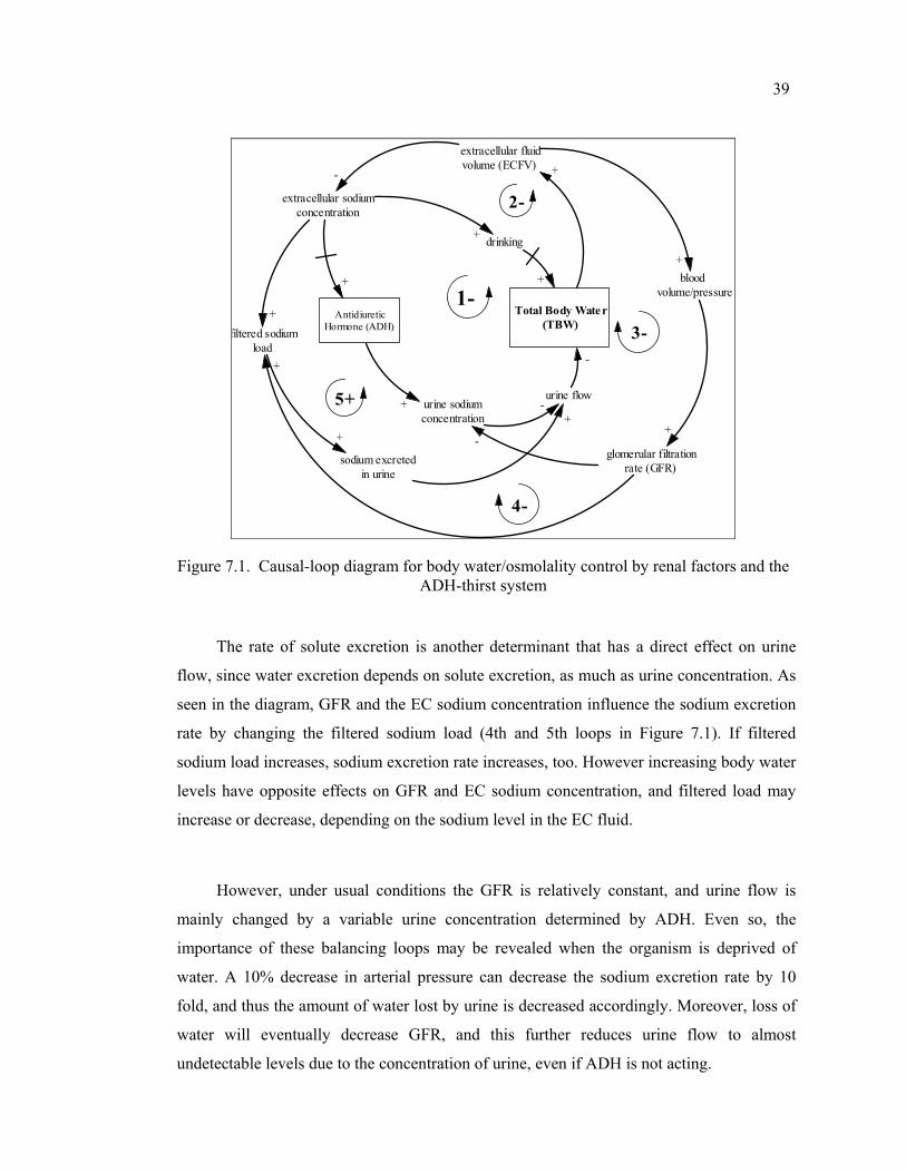
39
Total Body Water(TBW)
extracellular fluidvolume (ECFV) +
urine flow
sodium excretedin urine
extracellular sodiumconcentration
-
AntidiureticHormone (ADH)
+
1-
urine sodiumconcentration
drinking
+
2-
+
+
glomerular filtrationrate (GFR)
filtered sodiumload
+
+
4-
+
+
3--
-
-
bloodvolume/pressure
+
+
5+
Figure 7.1. Causal-loop diagram for body water/osmolality control by renal factors and the ADH-thirst system
The rate of solute excretion is another determinant that has a direct effect on urine
flow, since water excretion depends on solute excretion, as much as urine concentration. As
seen in the diagram, GFR and the EC sodium concentration influence the sodium excretion
rate by changing the filtered sodium load (4th and 5th loops in Figure 7.1). If filtered
sodium load increases, sodium excretion rate increases, too. However increasing body water
levels have opposite effects on GFR and EC sodium concentration, and filtered load may
increase or decrease, depending on the sodium level in the EC fluid.
However, under usual conditions the GFR is relatively constant, and urine flow is
mainly changed by a variable urine concentration determined by ADH. Even so, the
importance of these balancing loops may be revealed when the organism is deprived of
water. A 10% decrease in arterial pressure can decrease the sodium excretion rate by 10
fold, and thus the amount of water lost by urine is decreased accordingly. Moreover, loss of
water will eventually decrease GFR, and this further reduces urine flow to almost
undetectable levels due to the concentration of urine, even if ADH is not acting.
40
7.1.2. Control of Total Body Sodium and Extracellular Fluid Volume
Unlike the regulation of total body water via thirst-ADH mechanism, which is
comparatively well understood, the mechanisms involved in the regulation of Na+ and
thereby EC fluid volume (ECFV) remain controversial. This is mainly due to the diverse,
complex and interconnected nature of the factors that affect the Na+ balance.
Maintenance of normal ECFV and ECNa necessitates a balance between Na+ intake
and Na+ excretion. Under normal conditions, about 15% of body Na+ is turned over
between the gut and the plasma every day. So the amount which can be possibly lost to the
environment is very large when compared to the sodium stocks of the body. Therefore,
under normal conditions, more than 99% of sodium is reabsorbed back to the plasma (Bray
et al., 1989). If Na+ regulating mechanisms do not work appropriately, rapid loss of Na+
may lead to a rapid depletion of ECFV, hypotension, coma and death.
In modern industrialized cultures, Na+ intake is almost always greater than necessary
for homeostasis. In fact, the average sodium intake of modern civilizations usually ranges
between 100 and 200 mEq/day, even though humans can survive and function normally on
10 to 20 mEq/day (Guyton, 2000). The higher incidence of cardiovascular disorders such as
hypertension in modern civilizations is partly attributed to our usual high Na+ intake, and
most of the time it is not possible to control sodium balance by regulating intake (Navar,
1997). Therefore, the kidneys are left with the responsibility of adjusting the sodium
excretion rate against large variations in intake. However, it is also indicated that there is a
regulatory component to salt appetite, which works under extremely salt deficient
conditions such as in Addison’s disease, where the sodium retaining hormone ALD is
deficient in the body.
According to the most recent knowledge, sodium excretion mainly involves three
factors: the filtered load, ALD, and a group of ‘third factors’. Together with various other
factors, this system is capable to adjust the sodium excretion rate from a few mEq up to
about 500 mEq per day, which is a highly variable amount. Filtered load refers to the rate at
41
which substances are filtered in the kidney. It is found by the equation: Glomerular filtration
rate × plasma concentration of the substance, if it can be assumed that the substance is
freely filtered and not bound to any plasma proteins (Guyton, 2000). The other two
determinants of renal sodium loss, i.e. ALD, and “third factor” are hormones that retain or
excrete sodium by affecting the rate of its filtration and absorption. They also influence
other substances, e.g. glucose, water, and K+. The effects of the hormonal system on the
sodium balance will be outlined in Section 7.3.
As indicated above, three factors are identified to affect the renal sodium excretion.
Figure 7.2 provides a brief causal-loop diagram that demonstrates the causal mechanisms
related to these three factors. The 1st and the 3rd loops are related to balancing effects of
the filtered load. Any change that causes an increase in the filtered load of sodium causes a
rise in sodium excretion. It is seen that an increase in ECNa increases the filtered sodium
load both through an increased ECNa concentration, and an increased GFR. On the other
hand, the 2nd loop indicates that an increase in ECNa also has a decreasing effect on ECNa
concentration due to the fluid shift between the IC and the EC compartments. However, it is
apparent that the net effect of increased ECNa is a rise in ECNa concentration
(ECNa_conc), and thus the 2nd loops effect is always negated by the 1st loop, other things
being constant.
The 4th and 5th balancing feedback loops relate to the effects of ALD hormone. If the
ECNa level increases, this results in a fall in RA hormone levels, and a rise in ECNa
concentration. Sensing of this after a delay decreases the set level of the ALD hormone, and
consequently the sodium retaining effects of ALD decrease.
On the other hand, increasing levels of ECNa also trigger the natriuretic mechanisms.
Increasing EC fluid volume and the increased ratio of ECNa cause the set level of the ANH
to increase, which in turn results in an increased sodium excretion rate. As in the former
loops, the loops related to ANH (6th and 7th loops) also act in order to balance the change
in ECNa, and thus the ECFV and the blood volume levels.
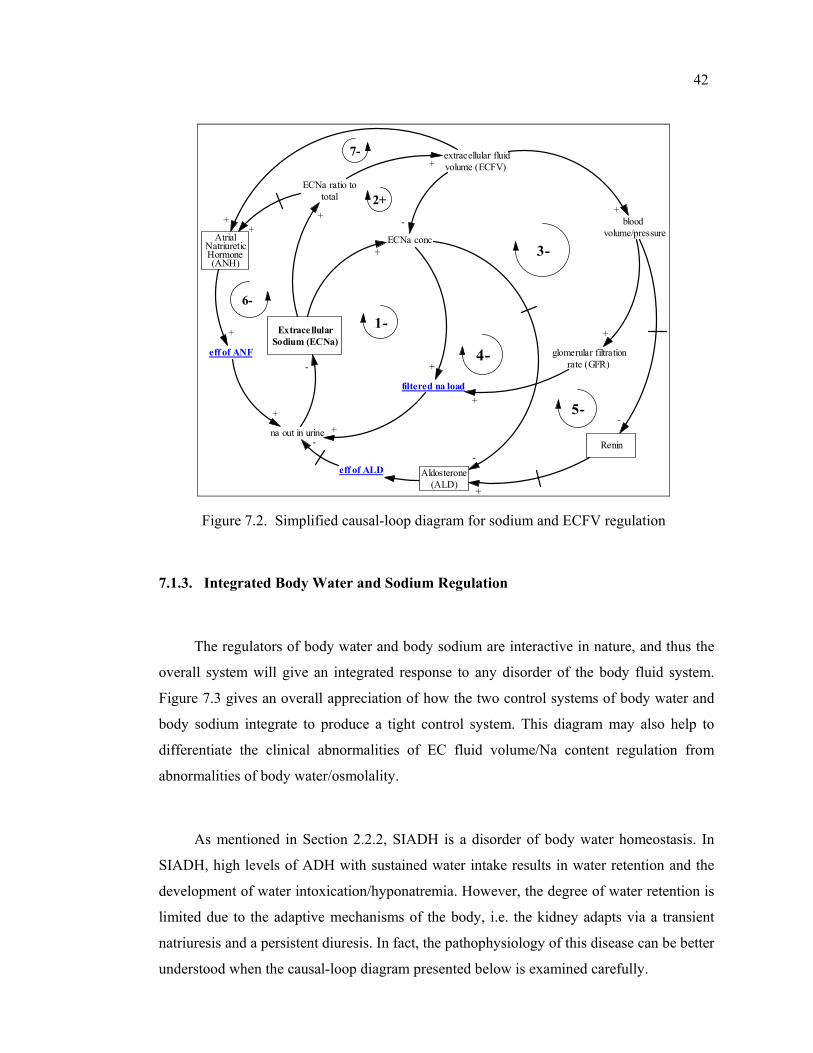
42
extracellular fluidvolume (ECFV)
Extrace llularSodium (ECNa)
ECNa conc
-Atrial
NatriureticHormone(ANH)
eff of ANF
+
6-
+
glomerular filtrationrate (GFR)
1-
filtered na load
+
3-
2+
+
bloodvolume/pressure
Aldosterone(ALD)
-
5-
4-
7-
+
eff of ALD
ECNa ratio tototal
+
++
na out in urine-
++
-
+
+
Renin
-
+
Figure 7.2. Simplified causal-loop diagram for sodium and ECFV regulation
7.1.3. Integrated Body Water and Sodium Regulation
The regulators of body water and body sodium are interactive in nature, and thus the
overall system will give an integrated response to any disorder of the body fluid system.
Figure 7.3 gives an overall appreciation of how the two control systems of body water and
body sodium integrate to produce a tight control system. This diagram may also help to
differentiate the clinical abnormalities of EC fluid volume/Na content regulation from
abnormalities of body water/osmolality.
As mentioned in Section 2.2.2, SIADH is a disorder of body water homeostasis. In
SIADH, high levels of ADH with sustained water intake results in water retention and the
development of water intoxication/hyponatremia. However, the degree of water retention is
limited due to the adaptive mechanisms of the body, i.e. the kidney adapts via a transient
natriuresis and a persistent diuresis. In fact, the pathophysiology of this disease can be better
understood when the causal-loop diagram presented below is examined carefully.
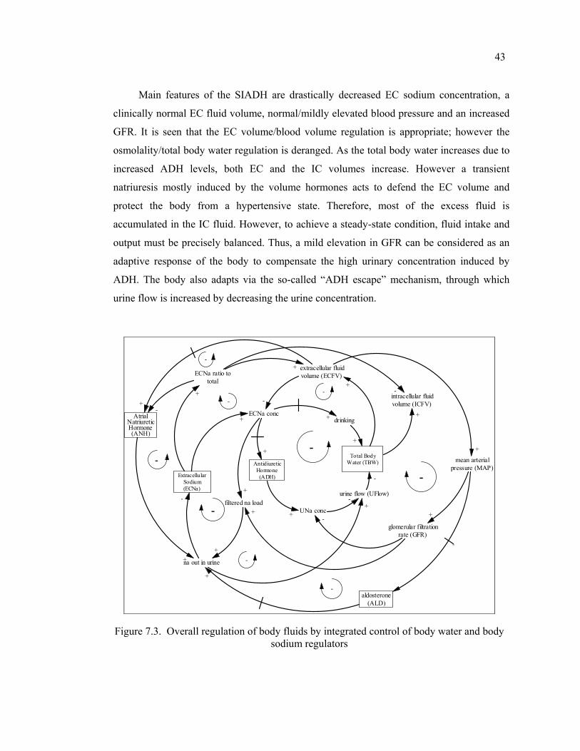
43
Main features of the SIADH are drastically decreased EC sodium concentration, a
clinically normal EC fluid volume, normal/mildly elevated blood pressure and an increased
GFR. It is seen that the EC volume/blood volume regulation is appropriate; however the
osmolality/total body water regulation is deranged. As the total body water increases due to
increased ADH levels, both EC and the IC volumes increase. However a transient
natriuresis mostly induced by the volume hormones acts to defend the EC volume and
protect the body from a hypertensive state. Therefore, most of the excess fluid is
accumulated in the IC fluid. However, to achieve a steady-state condition, fluid intake and
output must be precisely balanced. Thus, a mild elevation in GFR can be considered as an
adaptive response of the body to compensate the high urinary concentration induced by
ADH. The body also adapts via the so-called “ADH escape” mechanism, through which
urine flow is increased by decreasing the urine concentration.
Total BodyWater (TBW)
extracellular fluidvolume (ECFV)
+
urine flow (UFlow)
na out in urine
ExtracellularSodium(ECNa)
ECNa conc
-
-
AntidiureticHormone(ADH)
+
AtrialNatriureticHormone(ANH)
- -
+
UNa conc
drinking
+
-
+
+
glomerular filtrationrate (GFR)
-filtered na load
+
+
intracellular fluidvolume (ICFV)
+
-
-
ECNa ratio tototal
+
-
+
+
+
mean arterialpressure (MAP)
aldosterone(ALD)
+
-
--
-
-
-
-
+
-
+
+
+
Figure 7.3. Overall regulation of body fluids by integrated control of body water and body sodium regulators

44
In this chapter, each sector is explained in detail. For each sector, background
information and fundamental assumptions are given, main variables are defined and the
functions representing the relationships between variables are delineated.
In order to distinguish between the variables belonging to each sector, a prefix is used
while naming the variables. According to this convention Na stands for Sodium, EC stands
for Extracellular, IC stands for Intracellular, B stands for Blood, V stands for Volume, U
stands for Urine and Osm stands for Osmolality. For example ECNa_conc and UNa_conc
represent the Extracellular Sodium concentration and Urine Sodium Concentration,
respectively. Moreover, established abbreviations from the literature are used for some
variables. These are: ADH (Antidiuretic Hormone), ALD (Aldosterone Hormone), ANG
(Angiotensin Hormone), ANH (Atrial Natriuretic Hormone), GFR (Glomerular Filtration
Rate), and MAP (Mean Arterial Pressure).
7.2. Body Water Sector
7.2.1. Background Information
The absolute necessity of water in our physiological processes is beyond dispute,
since water is the medium in which all the chemical changes of the body occur. It is the
main constituent of digestive secretions, serves as a vehicle of absorption, is involved in the
composition of blood and lymph, is used as a lubricant in the body, plays an important role
in body temperature regulation, and so on…
However water is continuously escaping from the body, mostly through evaporation,
which creates a consequent need for repeated replenishment of body stores. Because of its
importance for life, the water conservation and replenishment mechanisms of the body
deserve a thorough investigation.
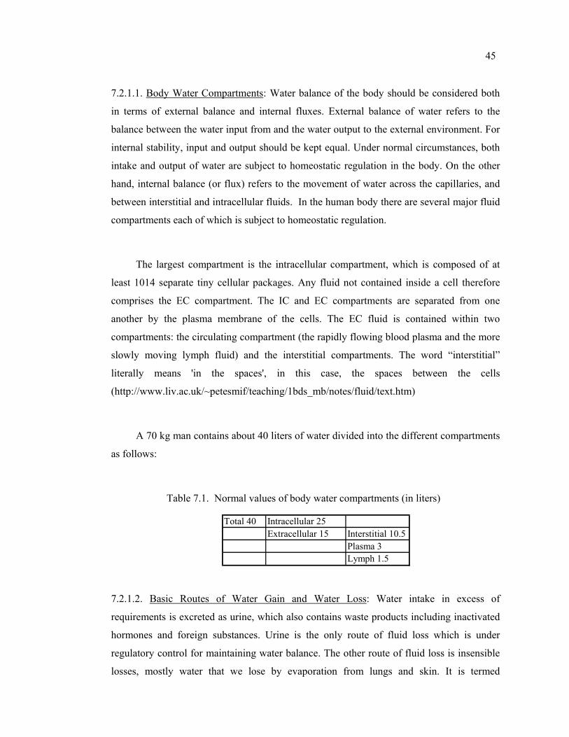
45
7.2.1.1. Body Water Compartments: Water balance of the body should be considered both
in terms of external balance and internal fluxes. External balance of water refers to the
balance between the water input from and the water output to the external environment. For
internal stability, input and output should be kept equal. Under normal circumstances, both
intake and output of water are subject to homeostatic regulation in the body. On the other
hand, internal balance (or flux) refers to the movement of water across the capillaries, and
between interstitial and intracellular fluids. In the human body there are several major fluid
compartments each of which is subject to homeostatic regulation.
The largest compartment is the intracellular compartment, which is composed of at
least 1014 separate tiny cellular packages. Any fluid not contained inside a cell therefore
comprises the EC compartment. The IC and EC compartments are separated from one
another by the plasma membrane of the cells. The EC fluid is contained within two
compartments: the circulating compartment (the rapidly flowing blood plasma and the more
slowly moving lymph fluid) and the interstitial compartments. The word “interstitial”
literally means 'in the spaces', in this case, the spaces between the cells
(http://www.liv.ac.uk/~petesmif/teaching/1bds_mb/notes/fluid/text.htm)
A 70 kg man contains about 40 liters of water divided into the different compartments
as follows:
Table 7.1. Normal values of body water compartments (in liters)
Total 40 Intracellular 25Extracellular 15 Interstitial 10.5
Plasma 3Lymph 1.5
7.2.1.2. Basic Routes of Water Gain and Water Loss: Water intake in excess of
requirements is excreted as urine, which also contains waste products including inactivated
hormones and foreign substances. Urine is the only route of fluid loss which is under
regulatory control for maintaining water balance. The other route of fluid loss is insensible
losses, mostly water that we lose by evaporation from lungs and skin. It is termed
46
'insensible' as we don’t sense this kind of water loss. The kidney is the major effector organ
in excreting urine, and it turns out that volume of urine (about 1 ml/min) is so much smaller
than that of plasma entering the kidneys each minute (about 650 ml/min). That means most
of the filtered amount will be reabsorbed back by renal mechanisms. The ADH-urinary
concentration mechanism will be explained in more detail in Sections 7.4 and 7.5.
Though ADH regulates the urine output by promoting concentration of urine; it
cannot reduce the urinary water output below a minimum level. Therefore, an additional
mechanism, i.e. thirst, is an integral part of the body water control. Thirst is a sensation of
land animals, which is more insistent and tormenting than hunger and it may be defined as
“the physiological urge to drink water”. The thirst mechanism is integrated with the ADH-
control mechanism. However, under usual conditions, most of the water intake is not due to
thirst, since human beings mostly drink according to their tastes and habits. This is termed
“secondary drinking”, which is not a result of a real thirst sensation. Therefore, thirst
functions as a backup effector mechanism.
7.2.2. Fundamental Approach and Assumptions
The total body water is contained within the numerous organs and tissues of the body.
However, theoretically we can divide it into compartments to gain physiological insight and
to predict some clinical measures. Thus, in this study we deal with idealized fluid
compartments which in fact do not exist as real entities. However, these compartments have
extremely important unifying similarities in terms of location, composition and behavior.
As mentioned before, the major division is into ICF and ECF which are separated by
the cell membrane. Another significant portion of the body water (15 % of total body water)
is contained in the fluid of bones and connective tissue; however this portion is excluded
from this study since it is a kinetically slow compartment. The transcellular fluids which are
small in volume are also ignored from the same reason. Consequently, this study only
considers those parts of the total body water that are rapidly equilibrating. The other most
important assumptions/rules related to the body water sector are as follows:
47
It is assumed that drinking, urinary excretion and insensible water loss need be
considered in calculating changes in overall body water control. Digestion and excretion of
food stuffs other than fluid and sodium ions, and the inflow of water gained by metabolic
oxidation are excluded.
The model of the water-drinking mechanism developed by Reeve and Kulhanek
(1967) forms the basis of the approach and assumptions regarding the drinking structure in
this study. Accordingly, drinking is considered as a constant or variable rate mechanism
governed by on-off switches and inhibitory feedback. The supposedly important effects of
habit on drinking behavior are ignored.
The urinary sodium concentration and the sodium excretion rate are selected as the
key indicators that affect the water excretion in urine. The underlying assumptions are: 1-
The rate of water transport is always proportional to the rate of solute transport and 2-The
urine flow is inversely related to the urinary concentration assuming a given sodium
outflow (Bray et al., 1989). Other mechanisms, such as neurological and psychological
influences, diurnal variation, etc. are not explicitly represented.
EC and IC compartments share the same osmolality. It is assumed that only water can
move freely between the IC and EC compartments to equalize their osmolalities, since
sodium and potassium are assumed to be locked in EC and IC compartments, respectively.
It is assumed that water is transferred between the EC and IC compartments instantaneously
to equalize their osmolalities, given the time units of the model.
The initial states and parameters are standard values which are quoted frequently in
the major medical textbooks and in earlier models. When available, published experimental
data is also used. The model assumes a standard healthy human male of approximately 70
kg with 40 liters of body water. The other factors causing variations in water content, i.e.
variation due to age, sex and degree of obesity is ignored, and average values are used.
48
7.2.3. Description of the Structure
As mentioned before, total body water content is controlled by a negative feedback
homeostatic mechanism which is often referred to by its effectors, i.e. the thirst-ADH
mechanism. This mechanism maintains total body water within narrow limits of as little as
+-0.5 L. of a mean (Reeve and Kulhanek, 1967). Moreover, the distribution of the body
water is also determined by this system. The structure constructed in this sector aims to
simulate the dynamics of the TBW and its compartments, i.e. the EC and the IC
compartments.
Stock flow diagram of the sector is given in Figure 7.4. Variables used in this sector
are presented in Appendix B with their brief descriptions and units.
The structure used for this sector includes three stock variables. Two of these stocks
represent the gut water and the body water, respectively. The third one is an artificial stock
which represents the drink mode (continuous and discrete), and will be explained later. The
only inflow of the gut water is drinking, which is defined as a constant or variable rate
mechanism governed by on-off switches and inhibitory feedback. The water absorbed from
the gut then will be distributed throughout the body. We assume that water transfer rate
from the gut to the interior is proportional to the amount currently in the gut. The time
constant to reach the interior body is selected as ½ hours, according to the observation that
there is a ½ to 1 hour delay for all of the water drunk to become uniformly distributed in the
body (Northrop, 2000).
Changes in the volume of TBW are the integral of all the rates of flow into and out of
the compartment. The two inflows of TBW are gut_to_in and water_infusion. Water
infusion flow is related to the treatment and will not be discussed here as the emphasis is on
normal physiology. The two outflows of the TBW stock are insensible loss, and urine flow.
Insensible loss refers to the amount of water lost by evaporation from lungs and skin
including fecal loss. This rate is assumed to have a constant value of about 0,9 L/day (Reeve
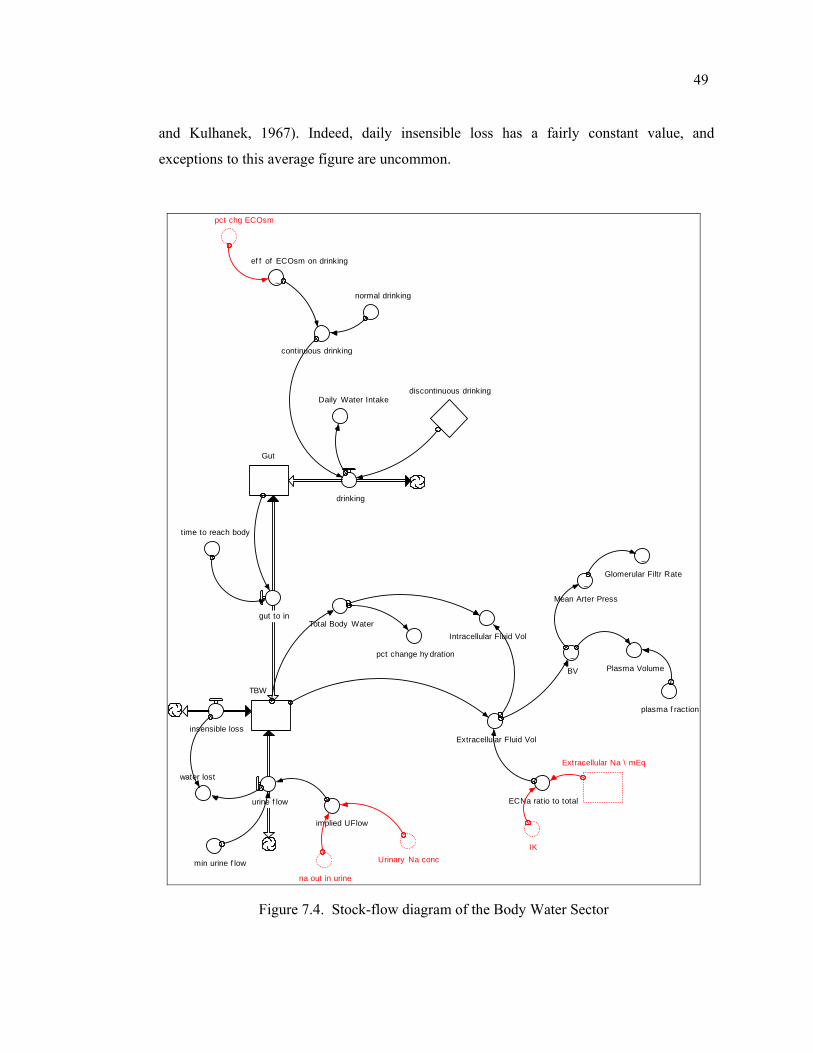
49
and Kulhanek, 1967). Indeed, daily insensible loss has a fairly constant value, and
exceptions to this average figure are uncommon.
TBW
urine f low
Extracellular Fluid Vol
Extracellular Na \ mEq
IK
~BV
discontinuous drinking
implied UFlow
~
ef f of ECOsm on drinking
Plasma Volume
min urine f low
Gut
gut to in
water lost
plasma f raction
drinking
insensible loss
pct chg ECOsm
pct change hy dration
~Glomerular Filtr Rate
time to reach body
Intracellular Fluid Vol
continuous drinking
normal drinking
~Mean Arter Press
Total Body Water
Daily Water Intake
na out in urine
ECNa ratio to total
Urinary Na conc
Figure 7.4. Stock-flow diagram of the Body Water Sector
50
The second outflow, i.e. the urinary water excretion, can be divided into a constant
rate and a variable “free water excretion”. This constant rate or the min_urine_flow is
referred as the obligatory urine loss, which is necessary to clear out the wasters of the body.
Instead of defining two different values for the urine flow, only one flow is used, and the
obligatory urine loss has been imposed as a constraint. Since the obligatory urine loss
approximates 500 ml per day, the min_urine_flow is defined as 0,3 ml/min. Consequently,
the equation for the urine_flow becomes:
_ (min_ _ , _ )urine flow MAX urine flow implied UFlow= (7.1)
The urine flow rate is in turn determined by two variables, i.e. the urinary sodium
concentration (UNa_conc), and the rate of sodium excretion (na_out_in_urine). The implied
urine flow rate is linearly related to sodium excretion, as the rate of water transport is
always proportional to the rate of solute transport. Accordingly, water excretion depends on
sodium excretion, since H2O ions passively follow Na+ ions, which are excreted by active
transport (Bray et al., 1989). The equation of the implied_UFlow is depicted below:
_ _ ___ 1000
na out in urineimplied UFlowUNa conc
=×
(7.2)
On the other hand, above equation depicts the inverse relationship between urine
osmolality and urine flow rate. Ordinarily the urine flow rate*urine osmolality (which
equals to the amount of solute excreted) is relatively constant and independent of flow rate,
as mentioned before. Thus the kidney can adjust the urine flow rate without markedly
affecting its handling of sodium, and the other solutes.
As mentioned before, the structure employed in this study considers drinking as the
main source of fluid intake, and both continuous and discontinuous drinking options are
modeled to simulate the drinking behavior of man. Discontinuous drinking of the model
represents a switch-on and switch off structure, which only acts under some threshold body
water level.
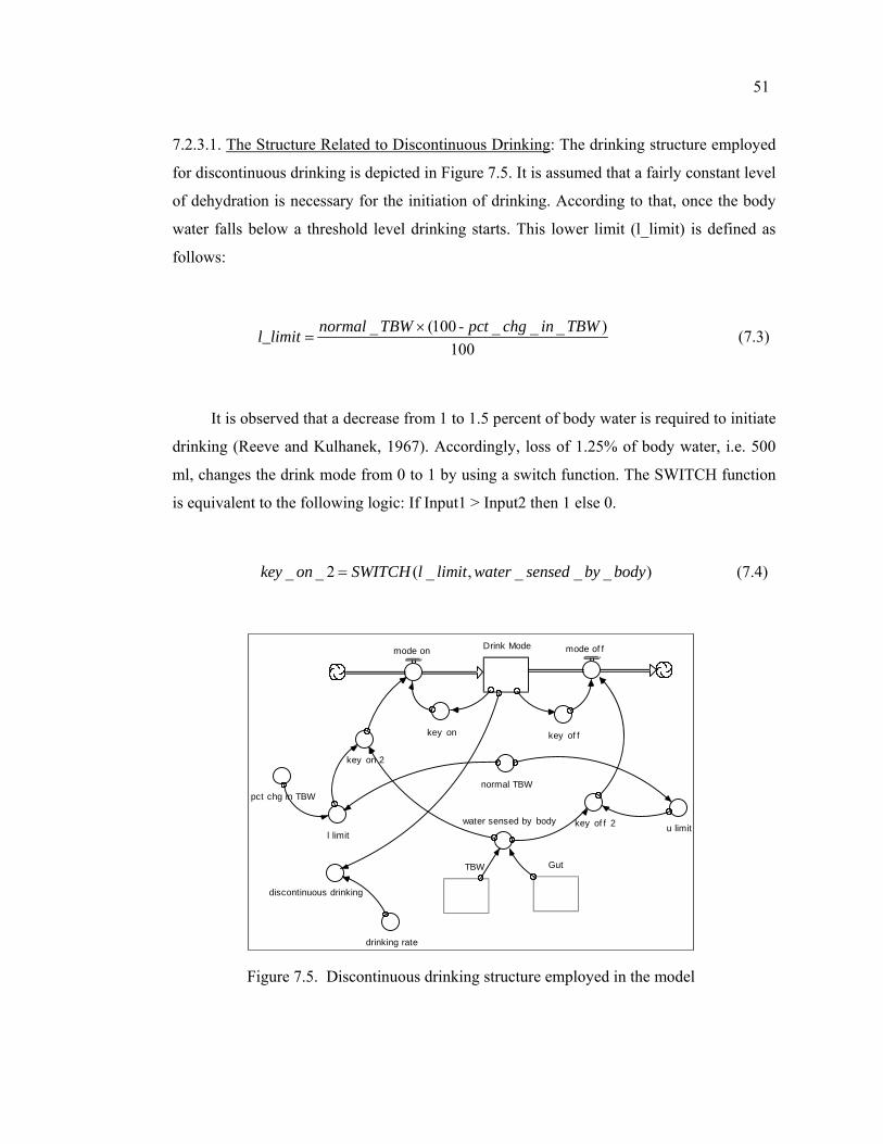
51
7.2.3.1. The Structure Related to Discontinuous Drinking: The drinking structure employed
for discontinuous drinking is depicted in Figure 7.5. It is assumed that a fairly constant level
of dehydration is necessary for the initiation of drinking. According to that, once the body
water falls below a threshold level drinking starts. This lower limit (l_limit) is defined as
follows:
_ (100 - _ _ _ )100
normal TBW pct chg in TBWl_limit ×= (7.3)
It is observed that a decrease from 1 to 1.5 percent of body water is required to initiate
drinking (Reeve and Kulhanek, 1967). Accordingly, loss of 1.25% of body water, i.e. 500
ml, changes the drink mode from 0 to 1 by using a switch function. The SWITCH function
is equivalent to the following logic: If Input1 > Input2 then 1 else 0.
_ _ 2 ( _ , _ _ _ )key on SWITCH l limit water sensed by body= (7.4)
discontinuous drinking
pct chg in TBW
Drink Modemode on mode of f
key on key of f
key of f 2
key on 2
water sensed by bodyl limit
u limit
drinking rate
normal TBW
TBW Gut
Figure 7.5. Discontinuous drinking structure employed in the model
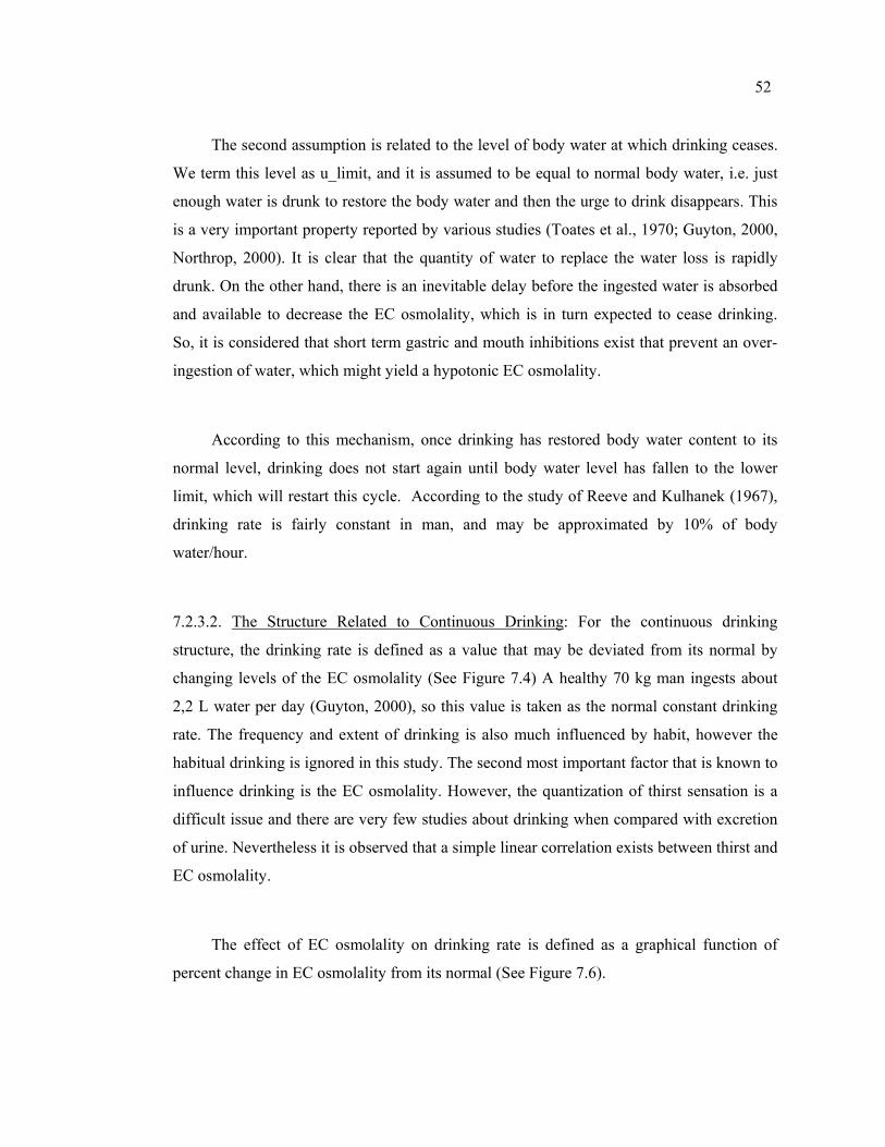
52
The second assumption is related to the level of body water at which drinking ceases.
We term this level as u_limit, and it is assumed to be equal to normal body water, i.e. just
enough water is drunk to restore the body water and then the urge to drink disappears. This
is a very important property reported by various studies (Toates et al., 1970; Guyton, 2000,
Northrop, 2000). It is clear that the quantity of water to replace the water loss is rapidly
drunk. On the other hand, there is an inevitable delay before the ingested water is absorbed
and available to decrease the EC osmolality, which is in turn expected to cease drinking.
So, it is considered that short term gastric and mouth inhibitions exist that prevent an over-
ingestion of water, which might yield a hypotonic EC osmolality.
According to this mechanism, once drinking has restored body water content to its
normal level, drinking does not start again until body water level has fallen to the lower
limit, which will restart this cycle. According to the study of Reeve and Kulhanek (1967),
drinking rate is fairly constant in man, and may be approximated by 10% of body
water/hour.
7.2.3.2. The Structure Related to Continuous Drinking: For the continuous drinking
structure, the drinking rate is defined as a value that may be deviated from its normal by
changing levels of the EC osmolality (See Figure 7.4) A healthy 70 kg man ingests about
2,2 L water per day (Guyton, 2000), so this value is taken as the normal constant drinking
rate. The frequency and extent of drinking is also much influenced by habit, however the
habitual drinking is ignored in this study. The second most important factor that is known to
influence drinking is the EC osmolality. However, the quantization of thirst sensation is a
difficult issue and there are very few studies about drinking when compared with excretion
of urine. Nevertheless it is observed that a simple linear correlation exists between thirst and
EC osmolality.
The effect of EC osmolality on drinking rate is defined as a graphical function of
percent change in EC osmolality from its normal (See Figure 7.6).
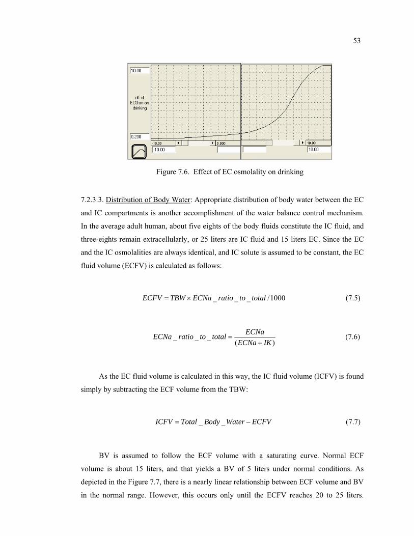
53
Figure 7.6. Effect of EC osmolality on drinking
7.2.3.3. Distribution of Body Water: Appropriate distribution of body water between the EC
and IC compartments is another accomplishment of the water balance control mechanism.
In the average adult human, about five eights of the body fluids constitute the IC fluid, and
three-eights remain extracellularly, or 25 liters are IC fluid and 15 liters EC. Since the EC
and the IC osmolalities are always identical, and IC solute is assumed to be constant, the EC
fluid volume (ECFV) is calculated as follows:
_ _ _ /1000ECFV TBW ECNa ratio to total= × (7.5)
_ _ _( )
ECNaECNa ratio to totalECNa IK
=+
(7.6)
As the EC fluid volume is calculated in this way, the IC fluid volume (ICFV) is found
simply by subtracting the ECF volume from the TBW:
_ _ICFV Total Body Water ECFV= − (7.7)
BV is assumed to follow the ECF volume with a saturating curve. Normal ECF
volume is about 15 liters, and that yields a BV of 5 liters under normal conditions. As
depicted in the Figure 7.7, there is a nearly linear relationship between ECF volume and BV
in the normal range. However, this occurs only until the ECFV reaches 20 to 25 liters.
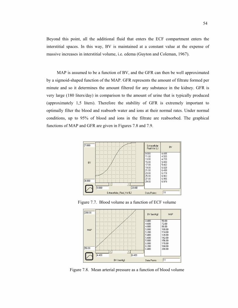
54
Beyond this point, all the additional fluid that enters the ECF compartment enters the
interstitial spaces. In this way, BV is maintained at a constant value at the expense of
massive increases in interstitial volume, i.e. edema (Guyton and Coleman, 1967).
MAP is assumed to be a function of BV, and the GFR can then be well approximated
by a sigmoid-shaped function of the MAP. GFR represents the amount of filtrate formed per
minute and so it determines the amount filtered for any substance in the kidney. GFR is
very large (180 liters/day) in comparison to the amount of urine that is typically produced
(approximately 1,5 liters). Therefore the stability of GFR is extremely important to
optimally filter the blood and reabsorb water and ions at their normal rates. Under normal
conditions, up to 95% of blood and ions in the filtrate are reabsorbed. The graphical
functions of MAP and GFR are given in Figures 7.8 and 7.9.
Figure 7.7. Blood volume as a function of ECF volume
Figure 7.8. Mean arterial pressure as a function of blood volume
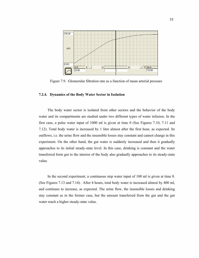
55
Figure 7.9. Glomerular filtration rate as a function of mean arterial pressure
7.2.4. Dynamics of the Body Water Sector in Isolation
The body water sector is isolated from other sectors and the behavior of the body
water and its compartments are studied under two different types of water infusion. In the
first case, a pulse water input of 1000 ml is given at time 0 (See Figures 7.10, 7.11 and
7.12). Total body water is increased by 1 liter almost after the first hour, as expected. Its
outflows, i.e. the urine flow and the insensible losses stay constant and cannot change in this
experiment. On the other hand, the gut water is suddenly increased and then it gradually
approaches to its initial steady-state level. In this case, drinking is constant and the water
transferred form gut to the interior of the body also gradually approaches to its steady-state
value.
In the second experiment, a continuous step water input of 100 ml is given at time 0.
(See Figures 7.13 and 7.14). After 4 hours, total body water is increased almost by 400 ml,
and continues to increase, as expected. The urine flow, the insensible losses and drinking
stay constant as in the former case, but the amount transferred from the gut and the gut
water reach a higher steady-state value.
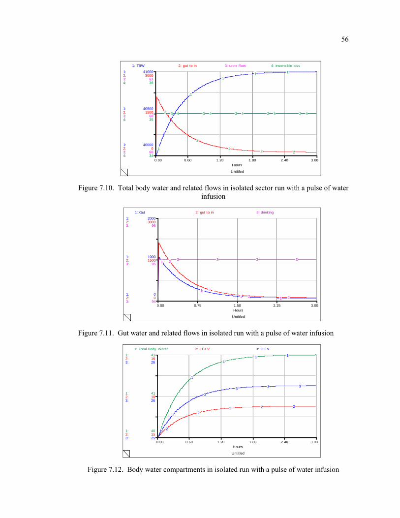
56
Untitled
0.00 0.60 1.20 1.80 2.40 3.00Hours
1:
1:
1:
2:
2:
2:
3:
3:
3:
4:
4:
4:
40000
40500
41000
0
1500
3000
60
60
61
34
35
36
1: TBW 2: gut to in 3: urine f low 4: insensible loss
1
1
11 1
2
2
22 2
3 3 3 3 34 4 4 4 4
Figure 7.10. Total body water and related flows in isolated sector run with a pulse of water infusion
Untitled
0.00 0.75 1.50 2.25 3.00Hours
1:
1:
1:
2:
2:
2:
3:
3:
3:
0
1000
2000
0
1500
3000
94
95
96
1: Gut 2: gut to in 3: drinking
1
1
1 1
2
2
2 2
3 3 3 3
Figure 7.11. Gut water and related flows in isolated run with a pulse of water infusion
Untitled
0.00 0.60 1.20 1.80 2.40 3.00Hours
1:
1:
1:
2:
2:
2:
3:
3:
3:
40
41
41
15
16
16
25
26
26
1: Total Body Water 2: ECFV 3: ICFV
1
1
11 1
2
22 2 2
3
33 3 3
Figure 7.12. Body water compartments in isolated run with a pulse of water infusion
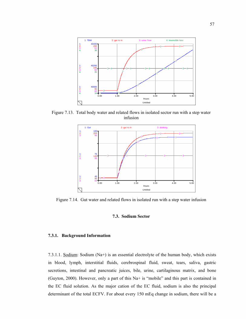
57
Untitled
0.00 1.00 2.00 3.00 4.00 5.00Hours
1:
1:
1:
2:
2:
2:
3:
3:
3:
4:
4:
4:
40000
40200
40400
90
145
200
60
60
61
34
35
36
1: TBW 2: gut to in 3: urine f low 4: insensible loss
1 1
1
1
1
2
2
22 2
3 3 3 3 34 4 4 4 4
Figure 7.13. Total body water and related flows in isolated sector run with a step water infusion
Untitled
0.00 1.00 2.00 3.00 4.00 5.00Hours
1:
1:
1:
2:
2:
2:
3:
3:
3:
45
75
105
90
145
200
94
95
96
1: Gut 2: gut to in 3: drinking
1
1
1
1 1
2
2
22 2
3 3 3 3 3
Figure 7.14. Gut water and related flows in isolated run with a step water infusion
7.3. Sodium Sector
7.3.1. Background Information
7.3.1.1. Sodium: Sodium (Na+) is an essential electrolyte of the human body, which exists
in blood, lymph, interstitial fluids, cerebrospinal fluid, sweat, tears, saliva, gastric
secretions, intestinal and pancreatic juices, bile, urine, cartilaginous matrix, and bone
(Guyton, 2000). However, only a part of this Na+ is “mobile” and this part is contained in
the EC fluid solution. As the major cation of the EC fluid, sodium is also the principal
determinant of the total ECFV. For about every 150 mEq change in sodium, there will be a
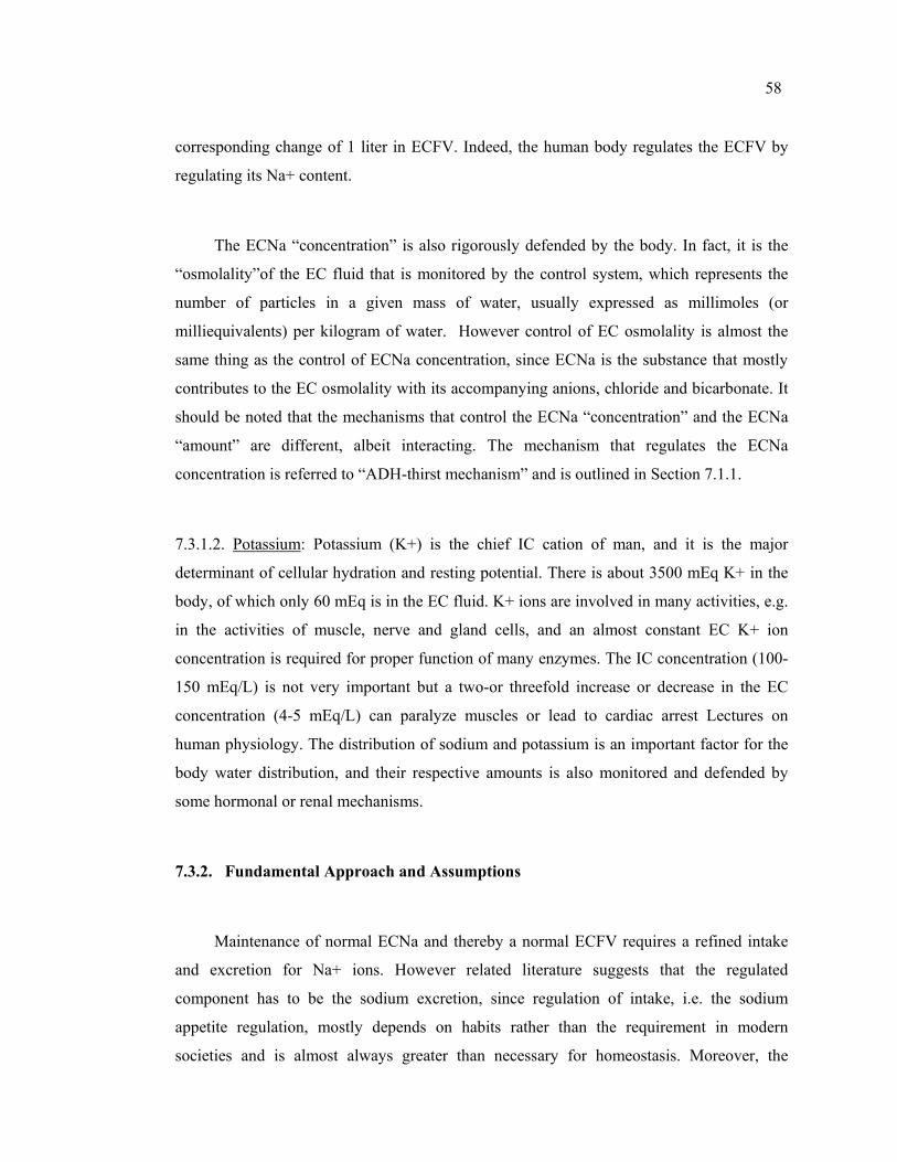
58
corresponding change of 1 liter in ECFV. Indeed, the human body regulates the ECFV by
regulating its Na+ content.
The ECNa “concentration” is also rigorously defended by the body. In fact, it is the
“osmolality”of the EC fluid that is monitored by the control system, which represents the
number of particles in a given mass of water, usually expressed as millimoles (or
milliequivalents) per kilogram of water. However control of EC osmolality is almost the
same thing as the control of ECNa concentration, since ECNa is the substance that mostly
contributes to the EC osmolality with its accompanying anions, chloride and bicarbonate. It
should be noted that the mechanisms that control the ECNa “concentration” and the ECNa
“amount” are different, albeit interacting. The mechanism that regulates the ECNa
concentration is referred to “ADH-thirst mechanism” and is outlined in Section 7.1.1.
7.3.1.2. Potassium: Potassium (K+) is the chief IC cation of man, and it is the major
determinant of cellular hydration and resting potential. There is about 3500 mEq K+ in the
body, of which only 60 mEq is in the EC fluid. K+ ions are involved in many activities, e.g.
in the activities of muscle, nerve and gland cells, and an almost constant EC K+ ion
concentration is required for proper function of many enzymes. The IC concentration (100-
150 mEq/L) is not very important but a two-or threefold increase or decrease in the EC
concentration (4-5 mEq/L) can paralyze muscles or lead to cardiac arrest Lectures on
human physiology. The distribution of sodium and potassium is an important factor for the
body water distribution, and their respective amounts is also monitored and defended by
some hormonal or renal mechanisms.
7.3.2. Fundamental Approach and Assumptions
Maintenance of normal ECNa and thereby a normal ECFV requires a refined intake
and excretion for Na+ ions. However related literature suggests that the regulated
component has to be the sodium excretion, since regulation of intake, i.e. the sodium
appetite regulation, mostly depends on habits rather than the requirement in modern
societies and is almost always greater than necessary for homeostasis. Moreover, the
59
mechanism for regulating intake are less understood and quantized. Therefore, the sodium
intake rate is assumed to be constant in the model and no behavioral changes are allowed.
For any substance, the amount of excreted in the urine is the algebraic sum of the
amounts filtered, reabsorbed and secreted by the tubules. As regarding sodium, only
filtration and reabsorption do exist since sodium is not secreted by tubules, e.g. unlike
potassium. The structure used in the model formulates sodium excretion rate as a value
which may deviate from its normal according to some factors, instead of first finding the
filtered amount and then subtract the reabsorbed portion. Sodium excretion is affected by
various factors; however only the most important ones, i.e. the GFR (which affects the
filtered load of sodium), the RAAS, plus the recently found ANH are explicitly represented
in the model. Other factors including the activation of the symphatetic nervous system,
which is indicated to have an important effect on sodium dynamics, is omitted and
considered to be constant. Moreover, sodium excretion rate is formulated to be independent
of urine flow, since neither the rate of solute reabsorption nor the total quantity of solute in
ECF is altered by changes in reabsorbed water. The importance and implications of this
feature will be explained in Section 7.5 in more detail
Another assumption is related to the distribution of sodium in the body. Most of the
mobile sodium that can vary in amount from day to day resides extracellularly, and only a
small portion resides in the cells. Another large amount is further contained in the bones;
however, this part does not contribute to the osmolality of the body fluids. As a result of
these, it is logical to assume that sodium is locked to the EC compartment. Similarly, the
major intracellular cation, i.e. potassium, is assumed to be locked to the intracellular
compartment, since only a small portion of potassium resides outside of the cells.
Furthermore, the amount of potassium is assumed to remain constant and cannot be changed
purposely, unlike the amount of sodium, which can be changed by addition or removal of
solute. The assumption that intracellular solute is constant is not always correct but these
special circumstances do not greatly detract from the general conclusion.
The second group of assumptions is associated with the “concentration” or
“osmolality” of sodium. First thing we have to note that it is the “tonicity”, and not
60
“osmolality”, which is the right term in the medical context. In fact, tonicity may be defined
as the effective osmolality and is equal to the sum of the concentrations of the solutes which
have the capacity to exert an osmotic force across the membrane, and the implication is that
tonicity is less then osmolality. Therefore whenever we use “osmolality”, we mean
“effective osmolality”, or “tonicity”.
One of the most important rules regarding the body fluids is that the EC and IC fluid
osmolalities (ECOsm and ICOsm) are always identical. In the model it is assumed that the
ECOsm is always proportional to EC sodium concentration and the ICOsm is proportional
to IC potassium concentration (Guyton, 2000). This is a logical assumption since sodium
ions of the ECF determine over 90 percent of the osmotic pressure of the ECF. The
contribution of two other solutes, glucose and urea, normally represent only 3 percent of the
total osmolality, and thus they are omitted. Consequently, the terms “control of sodium
concentration” and “control of osmolality” can be used at the same time and
interchangeably.
7.3.3. Description of the Structure
As mentioned before, regulation of sodium, water, and hormonal balances are
inextricably interdependent. However in this study they are constructed as single sectors to
increase readability. The structure constructed in this sector aims to simulate EC sodium
(ECNa) and the EC sodium concentration (ECNa_conc) dynamics which in turn have
profound effects on the body water distribution and the ECF volume.
Stock flow diagram of the sector is given in Figure 7.15. Brief descriptions of the
variables used in this sector are presented in Appendix B.
The structure used for this sector includes only one stock variable, which represents
the ECNa. This stock has a single inflow representing the normal sodium intake
(na_intake). As mentioned before, most people eat far more sodium than is necessary,
which usually ranges between 100 and 200 mEq/day. Accordingly, na_intake is defined as a
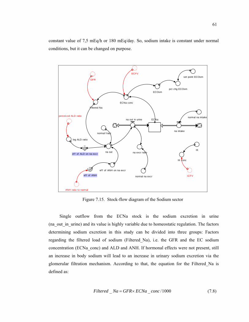
61
constant value of 7,5 mEq/h or 180 mEq/day. So, sodium intake is constant under normal
conditions, but it can be changed on purpose.
ECNa
IK
ICFV
na intake
na out in urinenormal na intake
IK conc
ECNa conc
normal f ract
na out
pct chg ECOsm
ef f of ANH on na excr
set point ECOsm
ANH ratio to normal
na excr ratio
perceiv ed ALD ratio
normal na excr
~ef f of ANH
ECFV~
GFR
Filtered Na
ECOsm
log ALD ratio
~ef f of ALD on na excr
Figure 7.15. Stock-flow diagram of the Sodium sector
Single outflow from the ECNa stock is the sodium excretion in urine
(na_out_in_urine) and its value is highly variable due to homeostatic regulation. The factors
determining sodium excretion in this study can be divided into three groups: Factors
regarding the filtered load of sodium (Filtered_Na), i.e. the GFR and the EC sodium
concentration (ECNa_conc) and ALD and ANH. If hormonal effects were not present, still
an increase in body sodium will lead to an increase in urinary sodium excretion via the
glomerular filtration mechanism. According to that, the equation for the Filtered_Na is
defined as:
_ _ /1000Filtered Na GFR ECNa conc= × (7.8)
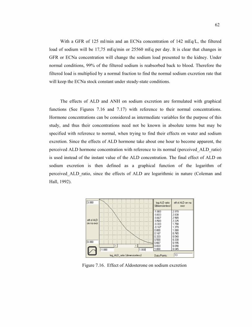
62
With a GFR of 125 ml/min and an ECNa concentration of 142 mEq/L, the filtered
load of sodium will be 17,75 mEq/min or 25560 mEq per day. It is clear that changes in
GFR or ECNa concentration will change the sodium load presented to the kidney. Under
normal conditions, 99% of the filtered sodium is reabsorbed back to blood. Therefore the
filtered load is multiplied by a normal fraction to find the normal sodium excretion rate that
will keep the ECNa stock constant under steady-state conditions.
The effects of ALD and ANH on sodium excretion are formulated with graphical
functions (See Figures 7.16 and 7.17) with reference to their normal concentrations.
Hormone concentrations can be considered as intermediate variables for the purpose of this
study, and thus their concentrations need not be known in absolute terms but may be
specified with reference to normal, when trying to find their effects on water and sodium
excretion. Since the effects of ALD hormone take about one hour to become apparent, the
perceived ALD hormone concentration with reference to its normal (perceived_ALD_ratio)
is used instead of the instant value of the ALD concentration. The final effect of ALD on
sodium excretion is then defined as a graphical function of the logarithm of
perceived_ALD_ratio, since the effects of ALD are logarithmic in nature (Coleman and
Hall, 1992).
Figure 7.16. Effect of Aldosterone on sodium excretion
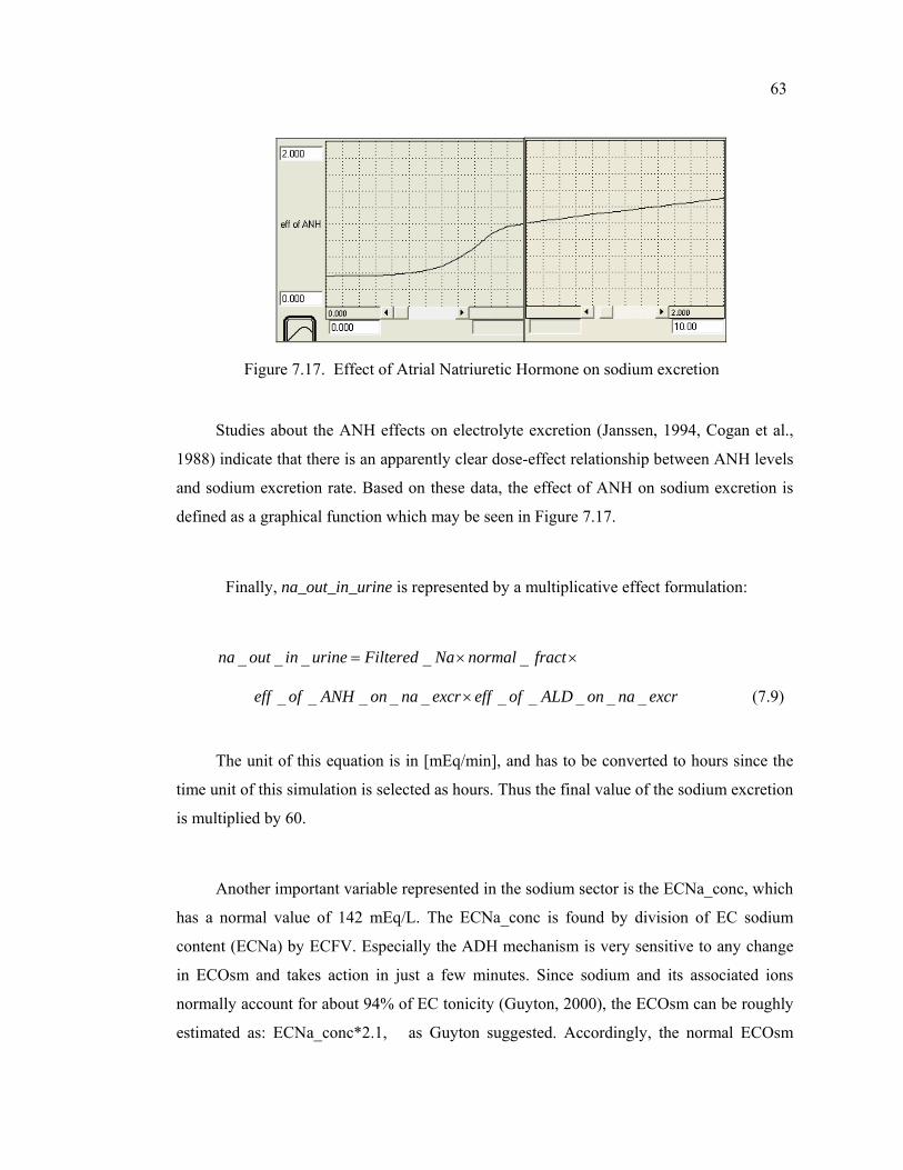
63
Figure 7.17. Effect of Atrial Natriuretic Hormone on sodium excretion
Studies about the ANH effects on electrolyte excretion (Janssen, 1994, Cogan et al.,
1988) indicate that there is an apparently clear dose-effect relationship between ANH levels
and sodium excretion rate. Based on these data, the effect of ANH on sodium excretion is
defined as a graphical function which may be seen in Figure 7.17.
Finally, na_out_in_urine is represented by a multiplicative effect formulation:
_ _ _ _ _na out in urine Filtered Na normal fract= × ×
_ _ _ _ _ _ _ _ _ _eff of ANH on na excr eff of ALD on na excr× (7.9)
The unit of this equation is in [mEq/min], and has to be converted to hours since the
time unit of this simulation is selected as hours. Thus the final value of the sodium excretion
is multiplied by 60.
Another important variable represented in the sodium sector is the ECNa_conc, which
has a normal value of 142 mEq/L. The ECNa_conc is found by division of EC sodium
content (ECNa) by ECFV. Especially the ADH mechanism is very sensitive to any change
in ECOsm and takes action in just a few minutes. Since sodium and its associated ions
normally account for about 94% of EC tonicity (Guyton, 2000), the ECOsm can be roughly
estimated as: ECNa_conc*2.1, as Guyton suggested. Accordingly, the normal ECOsm
64
would be estimated from the formula above to be about 298 mEq/ L, which is defined to be
the “set-point” for the ADH-thirst mechanism that controls the EC osmolality.
As mentioned before, the EC and the IC osmolalities are always identical after any
quick transients have passed. Since the amount of potassium (K) does not change in this
study, this quantity is represented simply by its normal physiological value of 3550 mEq,
and the ICOsm is taken as being proportional to intracellular potassium concentration
(ICK_conc). Similar to the ECNa concentration, the ICK_conc is found by division of IC
potassium content (ICK) by ICFV.
7.4. Endocrine System Sector Group
7.4.1. Background Information
The work of Guyton (2000) states that the functions of the body are regulated by two
major physiological systems: 1-the nervous system and 2-the endocrine (or hormonal)
system. Whereas the nervous system has a response time on the order of milliseconds, the
hormonal system shows a wide range of response time in exerting its functions. Hormones
are generally present in minute concentrations and are carried to their target organs in the
body by the circulatory system. Under usual circumstances secretion rates of all hormones
are under negative feedback loop control. The fact that the body water is a general
denominator in determining the electrolyte concentrations makes the hormonal system more
complex to understand (Northrop, 2000).
The kidney is the common site of action of these hormones, through which solutes
and water are excreted at variable rates, sometimes independently (Guyton, 2000). As a
consequence of this, hormonal functions are intimately interrelated through the functions of
the kidney, which plays a major role in the operation of all endogenous and hormonally
governed ionic regulatory systems. The major hormones regulating sodium and water
balance are the ADH, RAAS, and the more recently found ANH.
65
7.4.1.1. Antidiuretic Hormone (ADH): ADH is a neurohypophyseal hormone, which is
synthesized in the hypothalamus and deposited in the posterior pituitary gland as secretory
granules. It is known to play a major role in the regulation of water conservation in the
body. ADH is also often termed “vasopressin” due to its vasoconstrictive properties at
pharmacological high doses, and may also play a role in learning; memory and stress
response of the body. In the kidney, ADH exerts its function by increasing the permeability
of water in the nephrons, i.e. by promoting concentration of urine, and thus can control the
reabsorption of up to 10% of the filtered water (up to 10-20 liters per day!). Under normal
conditions, a change in ADH level immediately causes a change in urine flow and
osmolality (DeHaven and Shapiro, 1967). Figure 7.18 gives a schematic representation of
the normal physiologic relationships among EC osmolality (ECOsm), AVP (or ADH)
concentrations, urine osmolality (UOsm), and urine volume. Accordingly, UOsm is
proportional to plasma ADH levels, but urine volume is inversely related to urine
osmolality.
ADH deficiencies result in production of large amounts of urine that is maximally
dilute, a condition called Diabetes Insipidus (DI). On the other hand, excessive or
inappropriately high ADH levels result in water retention and development of water
intoxication/hyponatremia. The disorders related to ADH secretion and actions are
explained in Section 3.2.
The most important factors regulating ADH secretion are EC osmolality and effective
circulating blood volume. In contrast to the simple linear correlation between EC osmolality
and circulating ADH levels, the volume-ADH relationship is exponential, and may override
the osmotic effects in some conditions (See Figure 7.18). However blood volume decreases
in the order of 5 to 10 percent are necessary in order to activate the volume receptors,
whereas the osmoreceptors are sensitive to very minute changes in EC osmolality (Verbalis,
2003). The renal response to ADH is also similarly linear, since urinary concentration is
proportional to ADH levels. However a greater level of osmolality and subsequent ADH
release fails to increase urinary concentration when a certain threshold is reached. In
healthy individuals, this failure is compensated by the stimulation of thirst, and a potential
water deficit will be replenished. As a result, the rate of water intake and excretion is
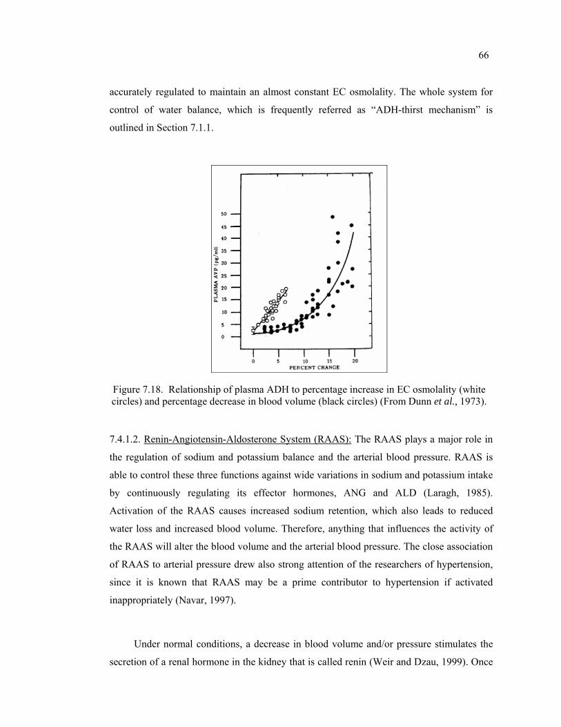
66
accurately regulated to maintain an almost constant EC osmolality. The whole system for
control of water balance, which is frequently referred as “ADH-thirst mechanism” is
outlined in Section 7.1.1.
Figure 7.18. Relationship of plasma ADH to percentage increase in EC osmolality (white circles) and percentage decrease in blood volume (black circles) (From Dunn et al., 1973).
7.4.1.2. Renin-Angiotensin-Aldosterone System (RAAS): The RAAS plays a major role in
the regulation of sodium and potassium balance and the arterial blood pressure. RAAS is
able to control these three functions against wide variations in sodium and potassium intake
by continuously regulating its effector hormones, ANG and ALD (Laragh, 1985).
Activation of the RAAS causes increased sodium retention, which also leads to reduced
water loss and increased blood volume. Therefore, anything that influences the activity of
the RAAS will alter the blood volume and the arterial blood pressure. The close association
of RAAS to arterial pressure drew also strong attention of the researchers of hypertension,
since it is known that RAAS may be a prime contributor to hypertension if activated
inappropriately (Navar, 1997).
Under normal conditions, a decrease in blood volume and/or pressure stimulates the
secretion of a renal hormone in the kidney that is called renin (Weir and Dzau, 1999). Once
67
in the blood stream, renin catalyzes a chemical process which ends with the production of
angiotensin II as an end product. ANG causes the kidneys to retain salt and water, both by
direct and indirect mechanisms. The indirect effect is mediated through ALD, a hormone
synthesized by the adrenal gland, for which release of angiotensin II is known as the most
potent direct stimulus (Other factors for ALD secretion are diminished EC sodium
concentration/sodium depletion, and increased EC potassium concentration). The second
mechanism is a direct effect on the kidneys, to cause reabsorption of sodium, and thus also
osmotic absorption of water.
In spite of its importance in sodium regulation, ALD is not the most important factor
to renal sodium excretion and thus EC fluid volume regulation, as supposed before.
Administration of excess amounts of ALD to a normal person produce salt and water
retention, but only for a finite period, after which “escape” from the effects of ALD occurs
and salt and water balance is maintained (Schrier and Niederberger, 1993). It is believed
that this escape mechanism accounts for the fact that patients with primary aldosteronism
(due to excess ALD levels) do not exhibit edema. The escape mechanism is considered to
be mediated by the “third factor”, namely by the ANH, which is explained below.
7.4.1.3. Atrial Natriuretic Hormone (ANH): Changes in sodium excretion, which could not
be explained either by changes in GFR or the ALD, were formerly attributed to an unknown
“third factor”, since it was seen that in the absence of change in both of these conditions,
saline loading was associated with an increase in sodium excretion. It has become clear that
this third factor is the ANH, which is secreted from the atrial tissue. The main factor for
ANH secretion is a rise in body fluid volumes, caused in a number of different ways, but
particularly by saline infusion Schrier et al., 1993, Yamasaki et al., 1988, Cogan et al.,
1988). This suggests that the distribution of water between EC and IC compartments is also
important in mediating secretion of ANH (Cameron, 1977), and thus one important function
of ANH could be to shift EC fluid from an overfilled vascular subcompartment to the
interstitial spaces in order to maintain a constant blood volume.
68
7.4.2. Fundamental Approach and Assumptions
Despite the intimately coupled relationships between sodium and water balance, we
can still classify their hormonal regulators as to their most important function. Accordingly,
the most important regulator of the water balance is the ADH-thirst mechanism, which is
studied extensively. This mechanism mainly controls the EC sodium concentration, and
therefore the distribution of body water between the compartments, as will be explained in
subsequent sections. However the regulation of sodium, i.e. the EC fluid volume regulation,
is less understood due to its complexity as to the water metabolism, and hormones that
affect sodium metabolism have been the focus of various investigations during this century.
In this study, the RAAS and the ANH are modeled as effector hormones of sodium
excretion, since their most important effect is on the sodium metabolism. These hormones
are also termed as “volume hormones”.
The main assumption related to the hormone sector is that the controllers, i.e.
hormones act according to set point theory. This assumption states that the rate of change of
all hormones is brought by deviations from set points. In this study, the set point is defined
in terms of concentration, i.e. the mechanism does not simply a change the “value” of the
corresponding hormone, but its “concentration”, since hormonal effects depend on
concentration rather than the absolute value.
Under normal conditions, all hormones are subject to diurnal variation, i.e. their blood
concentration fluctuates during the day. For example, ADH concentration in plasma
fluctuates with a maximum late at night and in the early morning and a minimum in the
early afternoon. This feature may be important while interpreting a hormone level, or when
prescribing a drug for the patient. Moreover, neurological and psychological influences may
also have important effects on hormone concentrations, even when any other thing seems to
be normal in the water and sodium balance. In this study, the diurnal variation, and
neurological and psychological influences are not explicitly represented and were
considered to be constant.
69
Another important assumption relates to the response time of the hormones. The
responses of ADH and ANH are assumed to take effect immediately, however ALD
responds to the value of stimuli after a delay. Therefore, ALD is important for long-term
rather than minute-to-minute adjustments of sodium excretion (Bray et al., 1989), whereas
ANH (together with changes in filtered load) is responsible for short term adjustments in
sodium excretion.
In this study, the RAAS is assumed to have only one effector hormone, namely the
ALD hormone. ANG is only considered as a hormone that stimulates ALD production.
Indeed, ANG is one of the most important determinants of ALD production; however ANG
itself also has been shown to regulate the rate of sodium reabsorption, independent of ALD.
In this study, the effects of ANG and ALD are lumped together and only the ALD effect is
represented explicitly.
Factors that cause secretion of hormones are also subject to controversy, and most of
the time the interdepence of water and sodium metabolism may blunt the real cause and
effect relationships between stimuli and response. Therefore quantitative results may vary
significantly between studies which are taken under different conditions and/or set of
assumptions. The factors chosen to effect hormone concentrations in this study will be
explained one by one in the next section.
7.4.3. Description of the Structure
The hormonal sector group is composed of three sectors, which are the ADH, RAAS,
and ANH. The structure constructed in these sectors is mainly responsible for simulating
the dynamics of the major hormones that are responsible for differential excretion of body
water and sodium ions.
All of these three sectors are mainly influenced by the feedbacks from the sodium and
body water sectors, and their output in turn determines the two most finely regulated
determinants of body water-electrolyte balance, i.e. the urinary concentration and the
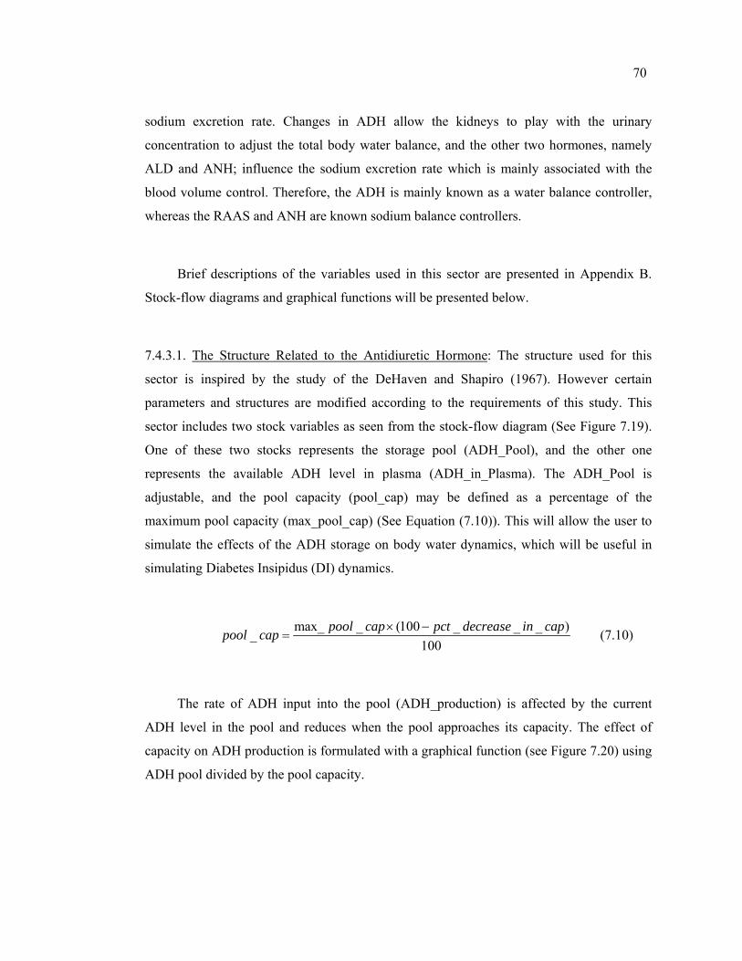
70
sodium excretion rate. Changes in ADH allow the kidneys to play with the urinary
concentration to adjust the total body water balance, and the other two hormones, namely
ALD and ANH; influence the sodium excretion rate which is mainly associated with the
blood volume control. Therefore, the ADH is mainly known as a water balance controller,
whereas the RAAS and ANH are known sodium balance controllers.
Brief descriptions of the variables used in this sector are presented in Appendix B.
Stock-flow diagrams and graphical functions will be presented below.
7.4.3.1. The Structure Related to the Antidiuretic Hormone: The structure used for this
sector is inspired by the study of the DeHaven and Shapiro (1967). However certain
parameters and structures are modified according to the requirements of this study. This
sector includes two stock variables as seen from the stock-flow diagram (See Figure 7.19).
One of these two stocks represents the storage pool (ADH_Pool), and the other one
represents the available ADH level in plasma (ADH_in_Plasma). The ADH_Pool is
adjustable, and the pool capacity (pool_cap) may be defined as a percentage of the
maximum pool capacity (max_pool_cap) (See Equation (7.10)). This will allow the user to
simulate the effects of the ADH storage on body water dynamics, which will be useful in
simulating Diabetes Insipidus (DI) dynamics.
max_ _ (100 _ _ _ )_100
pool cap pct decrease in cappool cap × −= (7.10)
The rate of ADH input into the pool (ADH_production) is affected by the current
ADH level in the pool and reduces when the pool approaches its capacity. The effect of
capacity on ADH production is formulated with a graphical function (see Figure 7.20) using
ADH pool divided by the pool capacity.
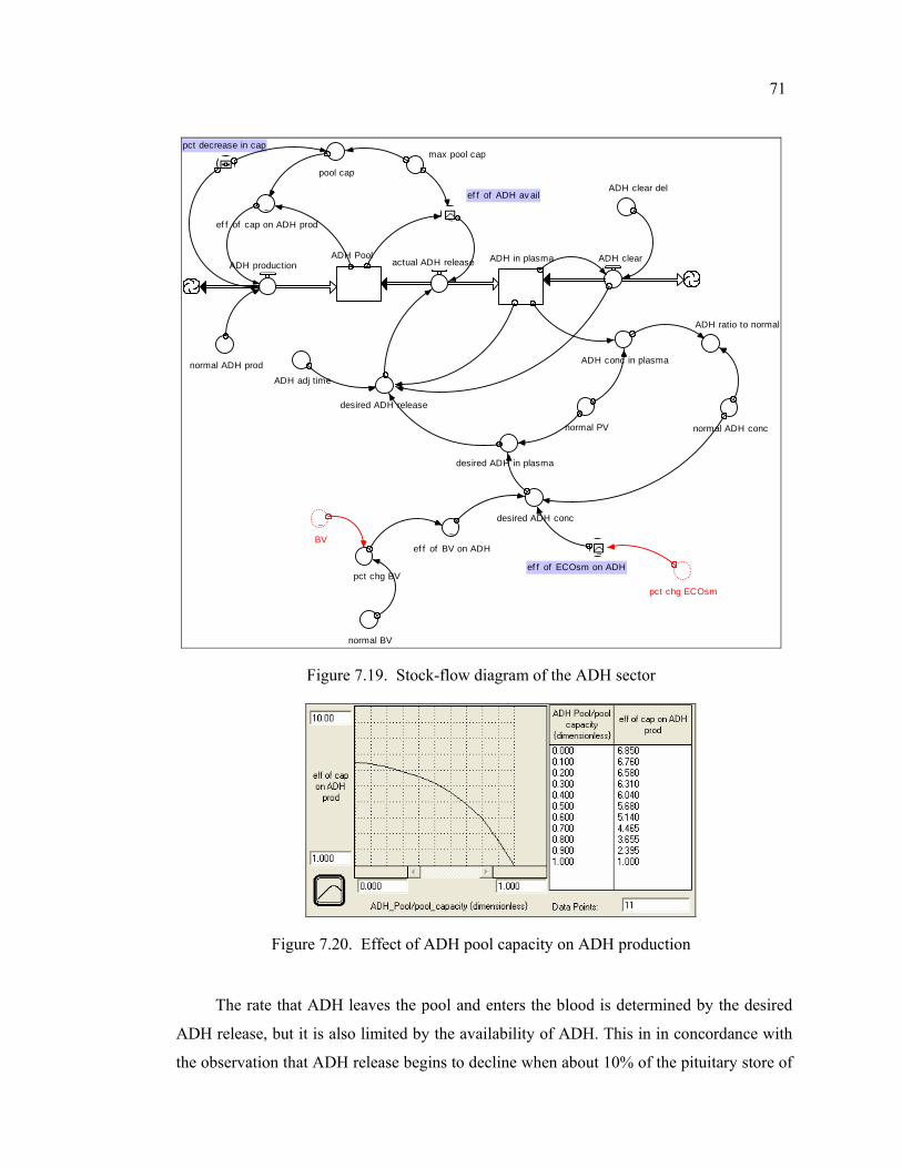
71
ADH Pool ADH in plasmaactual ADH release ADH clear
pct decrease in cap
desired ADH conc
ADH clear del
ADH conc in plasma
desired ADH in plasma
ADH ratio to normal
pct chg BV
normal ADH conc
ADH adj time
ADH production
pool cap
normal BV
normal PV
desired ADH release
~
ef f of ADH av ail
max pool cap
~BV
pct chg ECOsm
~ef f of BV on ADH ~
ef f of ECOsm on ADH
normal ADH prod
~ef f of cap on ADH prod
Figure 7.19. Stock-flow diagram of the ADH sector
Figure 7.20. Effect of ADH pool capacity on ADH production
The rate that ADH leaves the pool and enters the blood is determined by the desired
ADH release, but it is also limited by the availability of ADH. This in in concordance with
the observation that ADH release begins to decline when about 10% of the pituitary store of
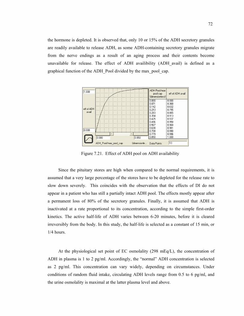
72
the hormone is depleted. It is observed that, only 10 or 15% of the ADH secretory granules
are readily available to release ADH, as some ADH-containing secretory granules migrate
from the nerve endings as a result of an aging process and their contents become
unavailable for release. The effect of ADH availibility (ADH_avail) is defined as a
graphical function of the ADH_Pool divided by the max_pool_cap.
Figure 7.21. Effect of ADH pool on ADH availability
Since the pituitary stores are high when compared to the normal requirements, it is
assumed that a very large percentage of the stores have to be depleted for the release rate to
slow down severely. This coincides with the observation that the effects of DI do not
appear in a patient who has still a partially intact ADH pool. The effects mostly appear after
a permanent loss of 80% of the secretory granules. Finally, it is assumed that ADH is
inactivated at a rate proportional to its concentration, according to the simple first-order
kinetics. The active half-life of ADH varies between 6-20 minutes, before it is cleared
irreversibly from the body. In this study, the half-life is selected as a constant of 15 min, or
1/4 hours.
At the physiological set point of EC osmolality (298 mEq/L), the concentration of
ADH in plasma is 1 to 2 pg/ml. Accordingly, the “normal” ADH concentration is selected
as 2 pg/ml. This concentration can vary widely, depending on circumstances. Under
conditions of random fluid intake, circulating ADH levels range from 0.5 to 6 pg/ml, and
the urine osmolality is maximal at the latter plasma level and above.
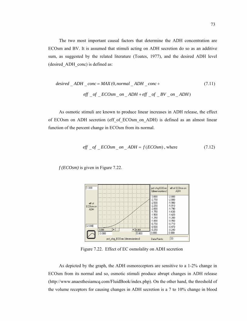
73
The two most important causal factors that determine the ADH concentration are
ECOsm and BV. It is assumed that stimuli acting on ADH secretion do so as an additive
sum, as suggested by the related literature (Toates, 1977), and the desired ADH level
(desired_ADH_conc) is defined as:
_ _ (0, _ _desired ADH conc MAX normal ADH conc= + (7.11)
_ _ _ _ _ _ _ _ )eff of ECOsm on ADH eff of BV on ADH+
As osmotic stimuli are known to produce linear increases in ADH release, the effect
of ECOsm on ADH secretion (eff_of_ECOsm_on_ADH) is defined as an almost linear
function of the percent change in ECOsm from its normal.
_ _ _ _ ( )eff of ECOsm on ADH f ECOsm= , where (7.12)
f (ECOsm) is given in Figure 7.22.
Figure 7.22. Effect of EC osmolality on ADH secretion
As depicted by the graph, the ADH osmoreceptors are sensitive to a 1-2% change in
ECOsm from its normal and so, osmotic stimuli produce abrupt changes in ADH release
(http://www.anaesthesiamcq.com/FluidBook/index.php). On the other hand, the threshold of
the volume receptors for causing changes in ADH secretion is a 7 to 10% change in blood
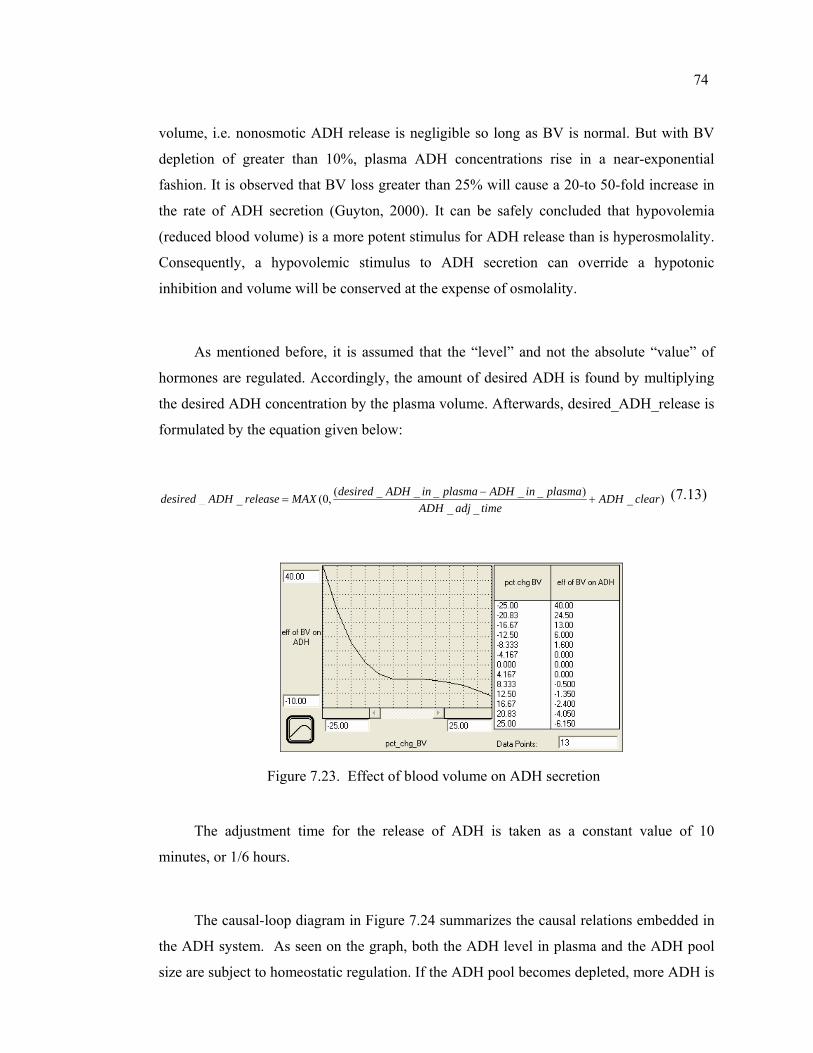
74
volume, i.e. nonosmotic ADH release is negligible so long as BV is normal. But with BV
depletion of greater than 10%, plasma ADH concentrations rise in a near-exponential
fashion. It is observed that BV loss greater than 25% will cause a 20-to 50-fold increase in
the rate of ADH secretion (Guyton, 2000). It can be safely concluded that hypovolemia
(reduced blood volume) is a more potent stimulus for ADH release than is hyperosmolality.
Consequently, a hypovolemic stimulus to ADH secretion can override a hypotonic
inhibition and volume will be conserved at the expense of osmolality.
As mentioned before, it is assumed that the “level” and not the absolute “value” of
hormones are regulated. Accordingly, the amount of desired ADH is found by multiplying
the desired ADH concentration by the plasma volume. Afterwards, desired_ADH_release is
formulated by the equation given below:
( _ _ _ _ _ )_ _ (0, _ )_ _
desired ADH in plasma ADH in plasmadesired ADH release MAX ADH clearADH adj time
−= + (7.13)
Figure 7.23. Effect of blood volume on ADH secretion
The adjustment time for the release of ADH is taken as a constant value of 10
minutes, or 1/6 hours.
The causal-loop diagram in Figure 7.24 summarizes the causal relations embedded in
the ADH system. As seen on the graph, both the ADH level in plasma and the ADH pool
size are subject to homeostatic regulation. If the ADH pool becomes depleted, more ADH is
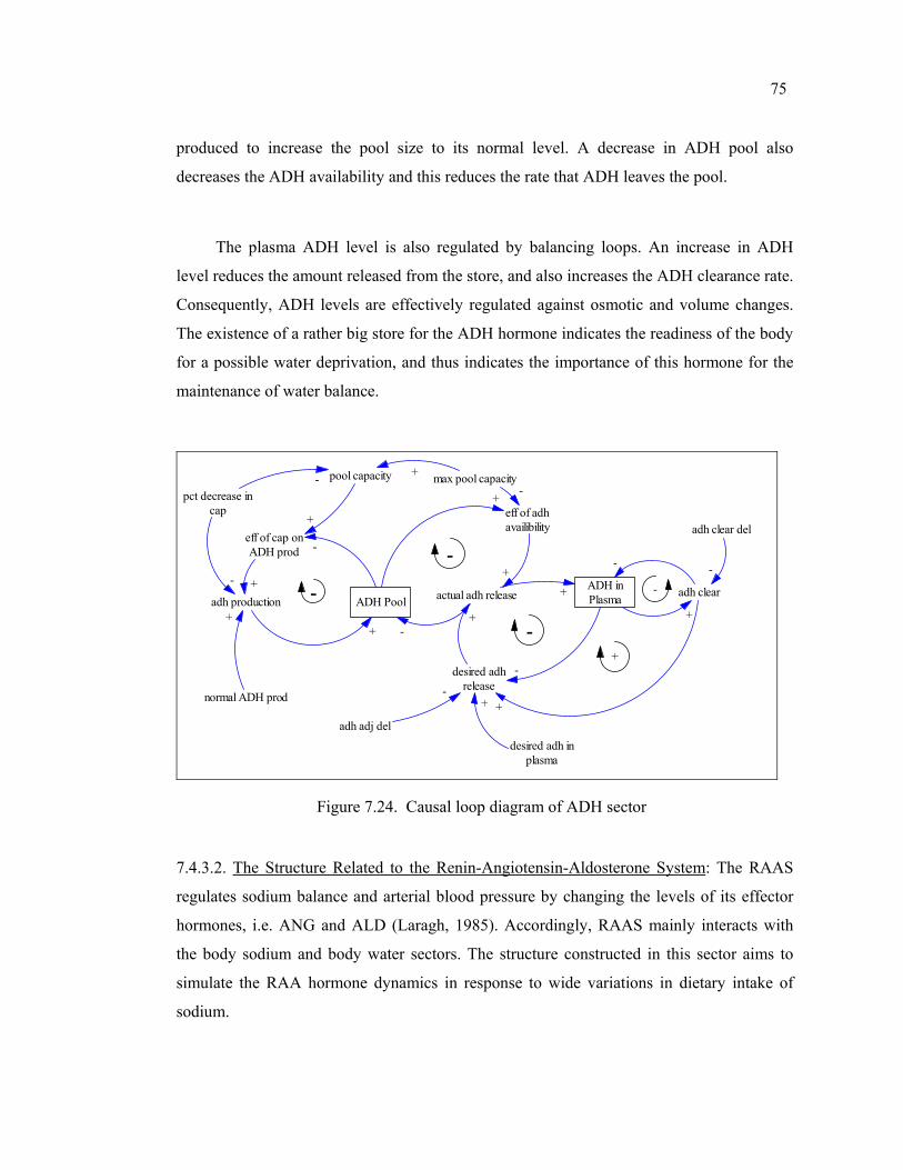
75
produced to increase the pool size to its normal level. A decrease in ADH pool also
decreases the ADH availability and this reduces the rate that ADH leaves the pool.
The plasma ADH level is also regulated by balancing loops. An increase in ADH
level reduces the amount released from the store, and also increases the ADH clearance rate.
Consequently, ADH levels are effectively regulated against osmotic and volume changes.
The existence of a rather big store for the ADH hormone indicates the readiness of the body
for a possible water deprivation, and thus indicates the importance of this hormone for the
maintenance of water balance.
adh production ADH Pool
pool capacity
eff of adhavailibility
actual adh releaseADH inPlasma adh clear
adh clear del
desired adhrelease
++
++
+
- -
-
adh adj deldesired adh in
plasma
+
-
-+
-+
--
pct decrease incap
eff of cap onADH prod
normal ADH prod
-
+
+
+
-
max pool capacity+-+ -
-
Figure 7.24. Causal loop diagram of ADH sector
7.4.3.2. The Structure Related to the Renin-Angiotensin-Aldosterone System: The RAAS
regulates sodium balance and arterial blood pressure by changing the levels of its effector
hormones, i.e. ANG and ALD (Laragh, 1985). Accordingly, RAAS mainly interacts with
the body sodium and body water sectors. The structure constructed in this sector aims to
simulate the RAA hormone dynamics in response to wide variations in dietary intake of
sodium.
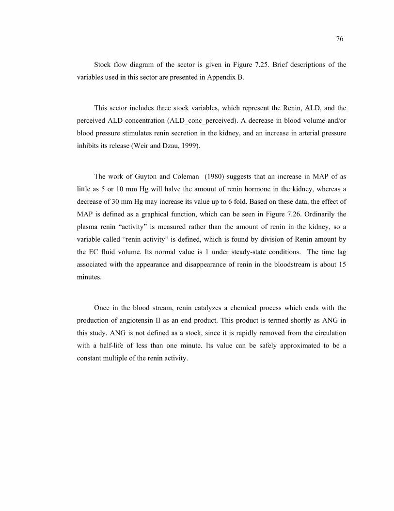
76
Stock flow diagram of the sector is given in Figure 7.25. Brief descriptions of the
variables used in this sector are presented in Appendix B.
This sector includes three stock variables, which represent the Renin, ALD, and the
perceived ALD concentration (ALD_conc_perceived). A decrease in blood volume and/or
blood pressure stimulates renin secretion in the kidney, and an increase in arterial pressure
inhibits its release (Weir and Dzau, 1999).
The work of Guyton and Coleman (1980) suggests that an increase in MAP of as
little as 5 or 10 mm Hg will halve the amount of renin hormone in the kidney, whereas a
decrease of 30 mm Hg may increase its value up to 6 fold. Based on these data, the effect of
MAP is defined as a graphical function, which can be seen in Figure 7.26. Ordinarily the
plasma renin “activity” is measured rather than the amount of renin in the kidney, so a
variable called “renin activity” is defined, which is found by division of Renin amount by
the EC fluid volume. Its normal value is 1 under steady-state conditions. The time lag
associated with the appearance and disappearance of renin in the bloodstream is about 15
minutes.
Once in the blood stream, renin catalyzes a chemical process which ends with the
production of angiotensin II as an end product. This product is termed shortly as ANG in
this study. ANG is not defined as a stock, since it is rapidly removed from the circulation
with a half-life of less than one minute. Its value can be safely approximated to be a
constant multiple of the renin activity.
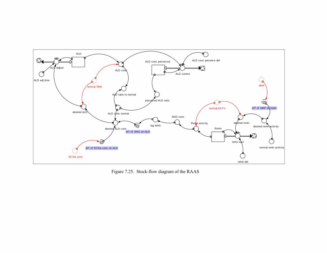
normal TBW
~MAP
normal ECFV
desired ALD conc
ALD ratio to normal
desired ALD
ALD
ALD adjust
ALD adj time
ALD conc
~ef f of ANG on ALD
ALD conc perceiv e del
ALD conc normal
ALD conc perceiv ed
ALD correct
ANG conc
log ANG
~ef f of MAP on renin
Renin
renin secr
normal renin activ ity
renin del
Renin activ itydesired renin activ ity
desired renin
perceiv ed ALD ratio
~ef f of ECNa conc on ALD
ECNa conc
Figure 7.25. Stock-flow diagram of the RAAS
78
Figure 7.26. Effect of mean arterial pressure on renin secretion
As mentioned before, the Renin-ANG system is assumed to function by changing the
rate of ALD secretion, i.e. the effects of ANG will appear indirectly. Secretion of ALD is
principally stimulated by the ANG level, and of lesser importance are decreased Na+ and
increased K+ concentrations in blood (Bray et al., 1989). ALD concentration is increased by
a rise in ANG and/or by a fall in EC sodium. However, it is not apparent whether the
increase in ALD secretion is a direct function of the decreased Na+ ion concentration itself
or is a result of some other effect associated with diminished total body sodium, since it is
almost impossible to deplete the body sodium without also decreasing the EC fluid volume
or without causing marked increase in renin activity. Quantitative estimations of the effect
of ECNa concentration on ALD secretion are also not very satisfactory. Guyton states that a
10 to 20% fall in ECNa concentration can rarely double the ALD level. However it is
known that severe hyponatremic patients have increased ALD levels despite of apparent
water retention.
The effects of ANG and ECNa concentration on ALD secretion are defined via
graphical functions which may be seen in Figures 7.27 and 7.28. Effect of ANG is defined
by using its logarithm, since most of the actions of the RAAS hormones are logarithmic in
nature (Coleman and Hall, 1992).
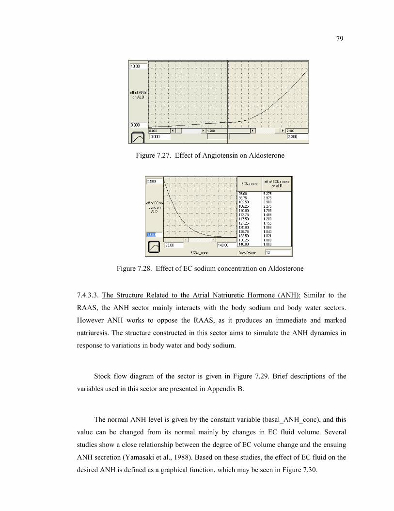
79
Figure 7.27. Effect of Angiotensin on Aldosterone
Figure 7.28. Effect of EC sodium concentration on Aldosterone
7.4.3.3. The Structure Related to the Atrial Natriuretic Hormone (ANH): Similar to the
RAAS, the ANH sector mainly interacts with the body sodium and body water sectors.
However ANH works to oppose the RAAS, as it produces an immediate and marked
natriuresis. The structure constructed in this sector aims to simulate the ANH dynamics in
response to variations in body water and body sodium.
Stock flow diagram of the sector is given in Figure 7.29. Brief descriptions of the
variables used in this sector are presented in Appendix B.
The normal ANH level is given by the constant variable (basal_ANH_conc), and this
value can be changed from its normal mainly by changes in EC fluid volume. Several
studies show a close relationship between the degree of EC volume change and the ensuing
ANH secretion (Yamasaki et al., 1988). Based on these studies, the effect of EC fluid on the
desired ANH is defined as a graphical function, which may be seen in Figure 7.30.
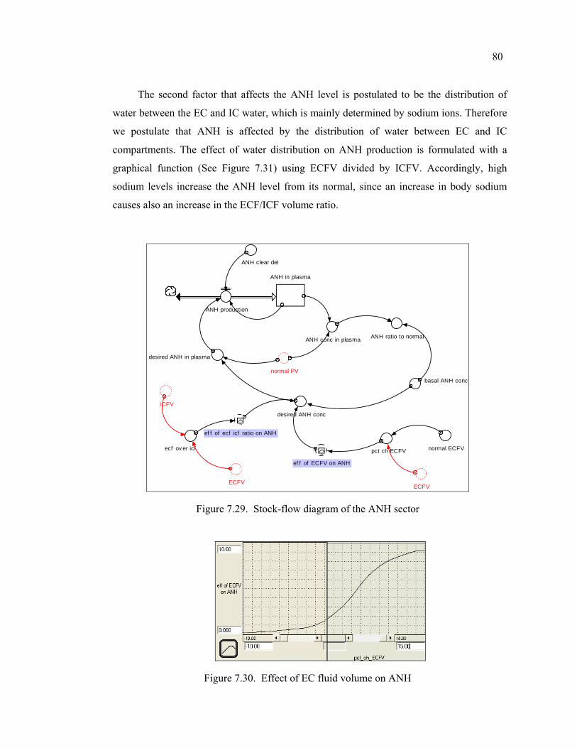
80
The second factor that affects the ANH level is postulated to be the distribution of
water between the EC and IC water, which is mainly determined by sodium ions. Therefore
we postulate that ANH is affected by the distribution of water between EC and IC
compartments. The effect of water distribution on ANH production is formulated with a
graphical function (See Figure 7.31) using ECFV divided by ICFV. Accordingly, high
sodium levels increase the ANH level from its normal, since an increase in body sodium
causes also an increase in the ECF/ICF volume ratio.
ECFV
ANH in plasma
ANH production
ANH clear del
desired ANH conc
normal PV
desired ANH in plasma
ecf ov er icf~
ef f of ECFV on ANH
ANH conc in plasma
ICFV
~ef f of ecf icf ratio on ANH
basal ANH conc
ANH ratio to normal
ECFV
pct ch ECFV normal ECFV
Figure 7.29. Stock-flow diagram of the ANH sector
Figure 7.30. Effect of EC fluid volume on ANH
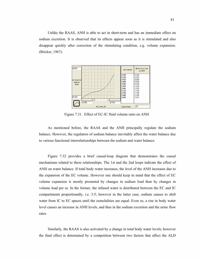
81
Unlike the RAAS, ANH is able to act in short-term and has an immediate effect on
sodium excretion. It is observed that its effects appear soon as it is stimulated and also
disappear quickly after correction of the stimulating condition, e.g. volume expansion.
(Bricker, 1967).
Figure 7.31. Effect of EC-IC fluid volume ratio on ANH
As mentioned before, the RAAS and the ANH principally regulate the sodium
balance. However, the regulators of sodium balance inevitably affect the water balance due
to various functional interrelationships between the sodium and water balance.
Figure 7.32 provides a brief causal-loop diagram that demonstrates the causal
mechanisms related to these relationships. The 1st and the 2nd loops indicate the effect of
ANH on water balance. If total body water increases, the level of the ANH increases due to
the expansion of the EC volume. However one should keep in mind that the effect of EC
volume expansion is mostly promoted by changes in sodium load than by changes in
volume load per se. In the former, the infused water is distributed between the EC and IC
compartments proportionally, i.e. 3:5; however in the latter case, sodium causes to shift
water from IC to EC spaces until the osmolalities are equal. Even so, a rise in body water
level causes an increase in ANH levels, and thus in the sodium excretion and the urine flow
rates.
Similarly, the RAAS is also activated by a change in total body water levels; however
the final effect is determined by a competition between two factors that affect the ALD
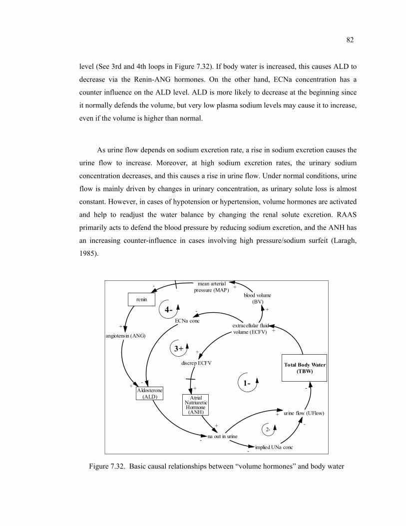
82
level (See 3rd and 4th loops in Figure 7.32). If body water is increased, this causes ALD to
decrease via the Renin-ANG hormones. On the other hand, ECNa concentration has a
counter influence on the ALD level. ALD is more likely to decrease at the beginning since
it normally defends the volume, but very low plasma sodium levels may cause it to increase,
even if the volume is higher than normal.
As urine flow depends on sodium excretion rate, a rise in sodium excretion causes the
urine flow to increase. Moreover, at high sodium excretion rates, the urinary sodium
concentration decreases, and this causes a rise in urine flow. Under normal conditions, urine
flow is mainly driven by changes in urinary concentration, as urinary solute loss is almost
constant. However, in cases of hypotension or hypertension, volume hormones are activated
and help to readjust the water balance by changing the renal solute excretion. RAAS
primarily acts to defend the blood pressure by reducing sodium excretion, and the ANH has
an increasing counter-influence in cases involving high pressure/sodium surfeit (Laragh,
1985).
Total Body Water(TBW)
extracellular fluidvolume (ECFV)
blood volume(BV)
+
urine flow (UFlow)
na out in urine
ECNa conc
-
AtrialNatriureticHormone(ANH)
1-
discrep ECFV
+
+
+
+
2-
mean arterialpressure (MAP) +
renin
-
angiotensin (ANG)
Aldosterone(ALD)
-
+
+
-
3+
4-
-
+
implied UNa conc-
-
Figure 7.32. Basic causal relationships between “volume hormones” and body water
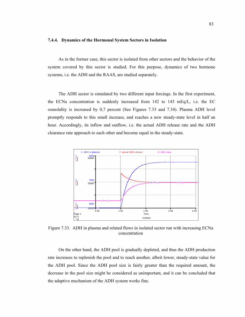
83
7.4.4. Dynamics of the Hormonal System Sectors in Isolation
As in the former case, this sector is isolated from other sectors and the behavior of the
system covered by this sector is studied. For this purpose, dynamics of two hormone
systems, i.e. the ADH and the RAAS, are studied separately.
The ADH sector is simulated by two different input forcings. In the first experiment,
the ECNa concentration is suddenly increased from 142 to 143 mEq/L, i.e. the EC
osmolality is increased by 0,7 percent (See Figures 7.33 and 7.34). Plasma ADH level
promptly responds to this small increase, and reaches a new steady-state level in half an
hour. Accordingly, its inflow and outflow, i.e. the actual ADH release rate and the ADH
clearance rate approach to each other and become equal in the steady-state.
Untitled
Page 10.50 1.00 1.50 2.00 2.50
Time
1:
1:
1:
2:
2:
2:
3:
3:
3:
6000
7500
9000
20000
35000
50000
1: ADH in plasma 2: actual ADH release 3: ADH clear
1
1
11
2
22 2
3
3
3 3
Figure 7.33. ADH in plasma and related flows in isolated sector run with increasing ECNa concentration
On the other hand, the ADH pool is gradually depleted, and thus the ADH production
rate increases to replenish the pool and to reach another, albeit lower, steady-state value for
the ADH pool. Since the ADH pool size is fairly greater than the required amount, the
decrease in the pool size might be considered as unimportant, and it can be concluded that
the adaptive mechanism of the ADH system works fine.
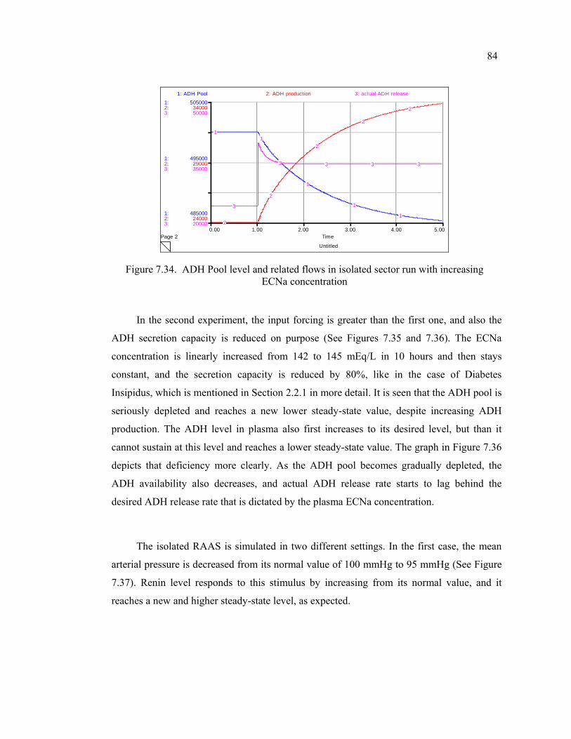
84
Untitled
Page 20.00 1.00 2.00 3.00 4.00 5.00
Time
1:
1:
1:
2:
2:
2:
3:
3:
3:
485000
495000
505000
24000
29000
34000
20000
35000
50000
1: ADH Pool 2: ADH production 3: actual ADH release
11
1
1
12
2
2
2
2
3
3 3 3 3
Figure 7.34. ADH Pool level and related flows in isolated sector run with increasing ECNa concentration
In the second experiment, the input forcing is greater than the first one, and also the
ADH secretion capacity is reduced on purpose (See Figures 7.35 and 7.36). The ECNa
concentration is linearly increased from 142 to 145 mEq/L in 10 hours and then stays
constant, and the secretion capacity is reduced by 80%, like in the case of Diabetes
Insipidus, which is mentioned in Section 2.2.1 in more detail. It is seen that the ADH pool is
seriously depleted and reaches a new lower steady-state value, despite increasing ADH
production. The ADH level in plasma also first increases to its desired level, but than it
cannot sustain at this level and reaches a lower steady-state value. The graph in Figure 7.36
depicts that deficiency more clearly. As the ADH pool becomes gradually depleted, the
ADH availability also decreases, and actual ADH release rate starts to lag behind the
desired ADH release rate that is dictated by the plasma ECNa concentration.
The isolated RAAS is simulated in two different settings. In the first case, the mean
arterial pressure is decreased from its normal value of 100 mmHg to 95 mmHg (See Figure
7.37). Renin level responds to this stimulus by increasing from its normal value, and it
reaches a new and higher steady-state level, as expected.
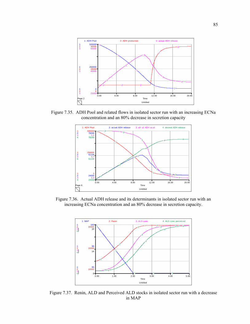
85
Untitled
Page 20.00 4.00 8.00 12.00 16.00 20.00
Time
1:
1:
1:
2:
2:
2:
3:
3:
3:
0
250000
500000
0
15000
30000
20000
40000
60000
1: ADH Pool 2: ADH production 3: actual ADH release
1
1
1
11
2 2 2
2
2
3
3
3
3
3
Figure 7.35. ADH Pool and related flows in isolated sector run with an increasing ECNa concentration and an 80% decrease in secretion capacity
Untitled
Page 60.00 4.00 8.00 12.00 16.00 20.00
Time
1:
1:
1:
2:
2:
2:
3:
3:
3:
4:
4:
4:
0
250000
500000
24000
51134
78269
0,4
0,7
1,0
24000
51134
78269
1: ADH Pool 2: actual ADH release 3: ef f of ADH av ail 4: desired ADH release
1
1
1
112
2
2
2
2
3 3
3
3
3
4
4
4
4 4
Figure 7.36. Actual ADH release and its determinants in isolated sector run with an increasing ECNa concentration and an 80% decrease in secretion capacity.
Untitled
0.00 1.00 2.00 3.00 4.00 5.00Time
1:
1:
1:
2:
2:
2:
3:
3:
3:
4:
4:
4:
95
98
100
10000
20000
30000
8
14
19
1: MAP 2: Renin 3: ALD conc 4: ALD conc perceiv ed
1
1
1 1 1
2
2
22 2
3
3
3
3 3
4
4
4
44
Figure 7.37. Renin, ALD and Perceived ALD stocks in isolated sector run with a decrease in MAP
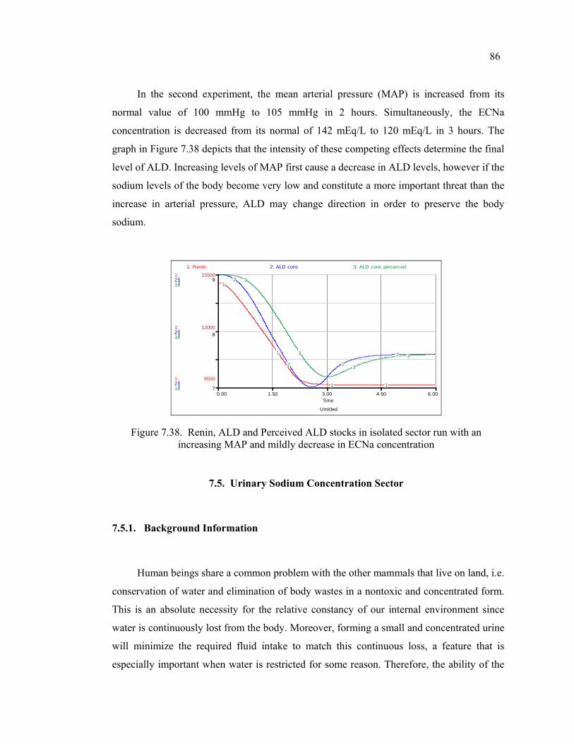
86
In the second experiment, the mean arterial pressure (MAP) is increased from its
normal value of 100 mmHg to 105 mmHg in 2 hours. Simultaneously, the ECNa
concentration is decreased from its normal of 142 mEq/L to 120 mEq/L in 3 hours. The
graph in Figure 7.38 depicts that the intensity of these competing effects determine the final
level of ALD. Increasing levels of MAP first cause a decrease in ALD levels, however if the
sodium levels of the body become very low and constitute a more important threat than the
increase in arterial pressure, ALD may change direction in order to preserve the body
sodium.
Untitled
0.00 1.50 3.00 4.50 6.00Time
1:
1:
1:
2:
2:
2:
3:
3:
3:
8500
12000
15500
7
8
9
1: Renin 2: ALD conc 3: ALD conc perceiv ed
1
1
1 1
2
2 2
2
3
3
3
3
Figure 7.38. Renin, ALD and Perceived ALD stocks in isolated sector run with an increasing MAP and mildly decrease in ECNa concentration
7.5. Urinary Sodium Concentration Sector
7.5.1. Background Information
Human beings share a common problem with the other mammals that live on land, i.e.
conservation of water and elimination of body wastes in a nontoxic and concentrated form.
This is an absolute necessity for the relative constancy of our internal environment since
water is continuously lost from the body. Moreover, forming a small and concentrated urine
will minimize the required fluid intake to match this continuous loss, a feature that is
especially important when water is restricted for some reason. Therefore, the ability of the
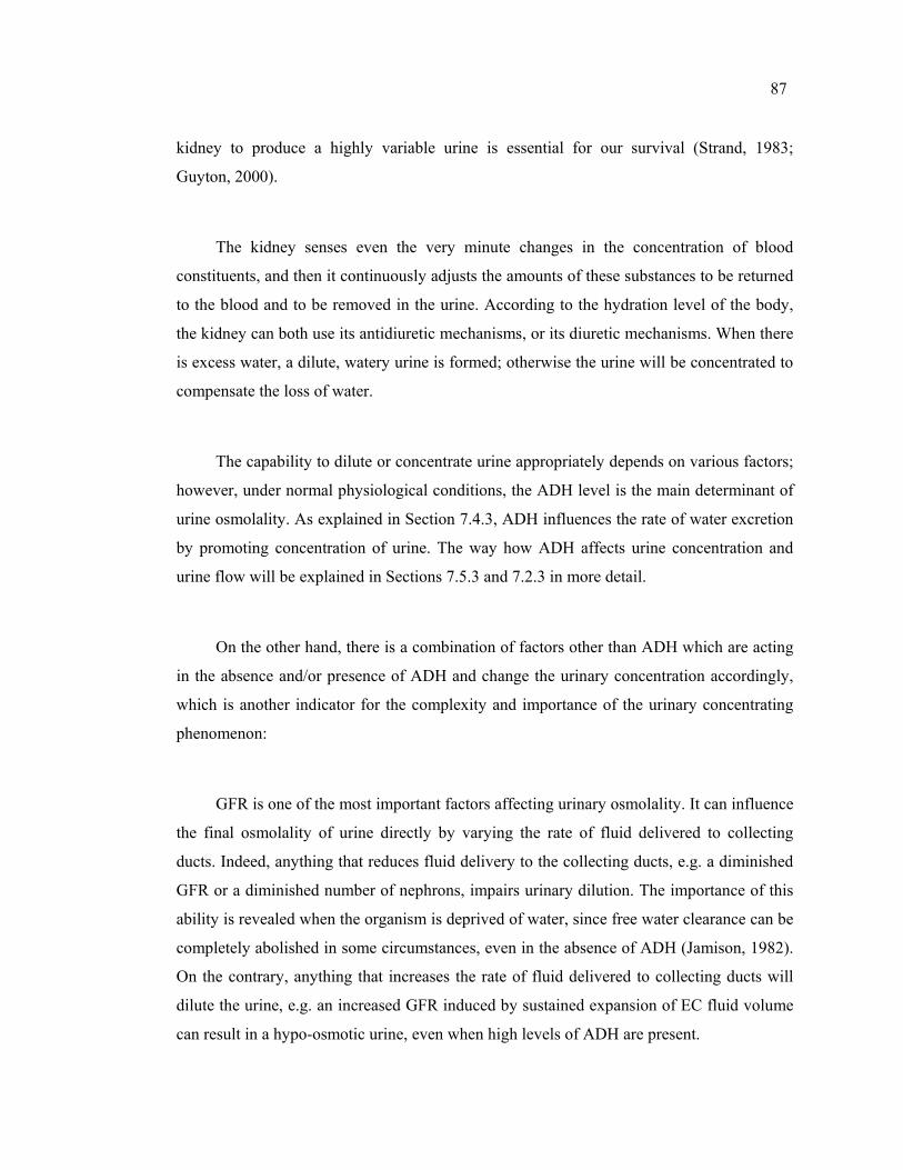
87
kidney to produce a highly variable urine is essential for our survival (Strand, 1983;
Guyton, 2000).
The kidney senses even the very minute changes in the concentration of blood
constituents, and then it continuously adjusts the amounts of these substances to be returned
to the blood and to be removed in the urine. According to the hydration level of the body,
the kidney can both use its antidiuretic mechanisms, or its diuretic mechanisms. When there
is excess water, a dilute, watery urine is formed; otherwise the urine will be concentrated to
compensate the loss of water.
The capability to dilute or concentrate urine appropriately depends on various factors;
however, under normal physiological conditions, the ADH level is the main determinant of
urine osmolality. As explained in Section 7.4.3, ADH influences the rate of water excretion
by promoting concentration of urine. The way how ADH affects urine concentration and
urine flow will be explained in Sections 7.5.3 and 7.2.3 in more detail.
On the other hand, there is a combination of factors other than ADH which are acting
in the absence and/or presence of ADH and change the urinary concentration accordingly,
which is another indicator for the complexity and importance of the urinary concentrating
phenomenon:
GFR is one of the most important factors affecting urinary osmolality. It can influence
the final osmolality of urine directly by varying the rate of fluid delivered to collecting
ducts. Indeed, anything that reduces fluid delivery to the collecting ducts, e.g. a diminished
GFR or a diminished number of nephrons, impairs urinary dilution. The importance of this
ability is revealed when the organism is deprived of water, since free water clearance can be
completely abolished in some circumstances, even in the absence of ADH (Jamison, 1982).
On the contrary, anything that increases the rate of fluid delivered to collecting ducts will
dilute the urine, e.g. an increased GFR induced by sustained expansion of EC fluid volume
can result in a hypo-osmotic urine, even when high levels of ADH are present.
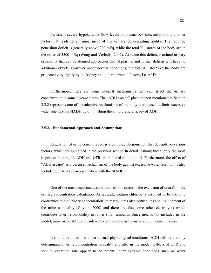
88
Persistent severe hypokalemia (low levels of plasma K+ concentration) is another
factor that leads to an impairment of the urinary concentrating ability. The required
potassium deficit is generally above 200 mEq, while the total K+ stores of the body are in
the order of 3500 mEq (Wong and Verbalis, 2002). At twice this deficit, maximal urinary
osmolality that can be attained approaches that of plasma, and further deficits will have no
additional effects. However under normal conditions, the total K+ stores of the body are
protected very tightly by the kidney and other hormonal factors, i.e. ALD.
Furthermore, there are some internal mechanisms that can affect the urinary
concentration in some disease states. The “ADH escape” phenomenon mentioned in Section
2.2.2 represents one of the adaptive mechanisms of the body that is used to limit excessive
water retention in SIADH by diminishing the antidiuretic efficacy of ADH.
7.5.2. Fundamental Approach and Assumptions
Regulation of urine concentration is a complex phenomenon that depends on various
factors, which are explained in the previous section in detail. Among these, only the most
important factors, i.e. ADH and GFR are included in the model. Furthermore, the effect of
“ADH escape” as a defense mechanism of the body against excessive water retention is also
included due to its close association with the SIADH.
One of the most important assumptions of this sector is the exclusion of urea from the
urinary concentration calculation. As a result, sodium chloride is assumed to be the only
contributor to the urinary concentration. In reality, urea also contributes about 40 percent of
the urine osmolality (Guyton, 2000) and there are also some other electrolytes which
contribute to urine osmolality in rather small amounts. Since urea is not included in the
model, urine osmolality is considered to be the same as the urine sodium concentration.
It should be noted that under normal physiological conditions, ADH will be the only
determinant of urine concentration in reality and also in the model. Effects of GFR and
sodium excretion rate appear to be potent under extreme conditions such as water
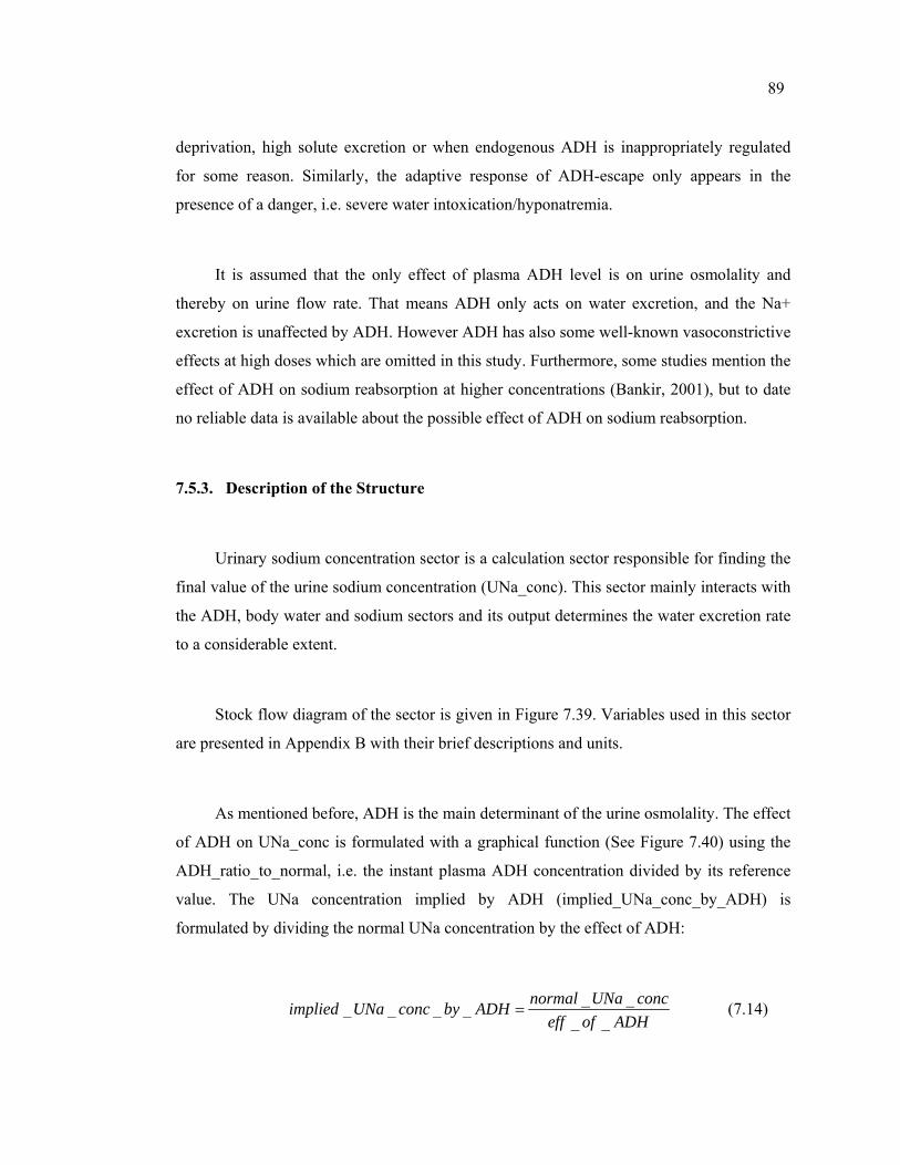
89
deprivation, high solute excretion or when endogenous ADH is inappropriately regulated
for some reason. Similarly, the adaptive response of ADH-escape only appears in the
presence of a danger, i.e. severe water intoxication/hyponatremia.
It is assumed that the only effect of plasma ADH level is on urine osmolality and
thereby on urine flow rate. That means ADH only acts on water excretion, and the Na+
excretion is unaffected by ADH. However ADH has also some well-known vasoconstrictive
effects at high doses which are omitted in this study. Furthermore, some studies mention the
effect of ADH on sodium reabsorption at higher concentrations (Bankir, 2001), but to date
no reliable data is available about the possible effect of ADH on sodium reabsorption.
7.5.3. Description of the Structure
Urinary sodium concentration sector is a calculation sector responsible for finding the
final value of the urine sodium concentration (UNa_conc). This sector mainly interacts with
the ADH, body water and sodium sectors and its output determines the water excretion rate
to a considerable extent.
Stock flow diagram of the sector is given in Figure 7.39. Variables used in this sector
are presented in Appendix B with their brief descriptions and units.
As mentioned before, ADH is the main determinant of the urine osmolality. The effect
of ADH on UNa_conc is formulated with a graphical function (See Figure 7.40) using the
ADH_ratio_to_normal, i.e. the instant plasma ADH concentration divided by its reference
value. The UNa concentration implied by ADH (implied_UNa_conc_by_ADH) is
formulated by dividing the normal UNa concentration by the effect of ADH:
_ __ _ _ __ _
normal UNa concimplied UNa conc by ADHeff of ADH
= (7.14)
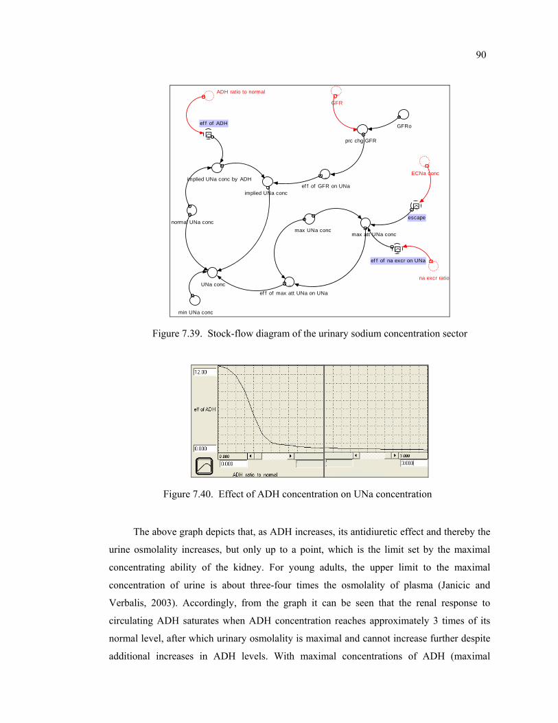
90
implied UNa conc
normal UNa conc
GFRo
~
ef f of ADH
min UNa conc
ADH ratio to normal
max att UNa conc
~ef f of na excr on UNa
~GFR
max UNa conc
na excr ratio
prc chg GFR
ECNa conc
~escape
~ef f of max att UNa on UNa
UNa conc
implied UNa conc by ADH ~ef f of GFR on UNa
Figure 7.39. Stock-flow diagram of the urinary sodium concentration sector
Figure 7.40. Effect of ADH concentration on UNa concentration
The above graph depicts that, as ADH increases, its antidiuretic effect and thereby the
urine osmolality increases, but only up to a point, which is the limit set by the maximal
concentrating ability of the kidney. For young adults, the upper limit to the maximal
concentration of urine is about three-four times the osmolality of plasma (Janicic and
Verbalis, 2003). Accordingly, from the graph it can be seen that the renal response to
circulating ADH saturates when ADH concentration reaches approximately 3 times of its
normal level, after which urinary osmolality is maximal and cannot increase further despite
additional increases in ADH levels. With maximal concentrations of ADH (maximal
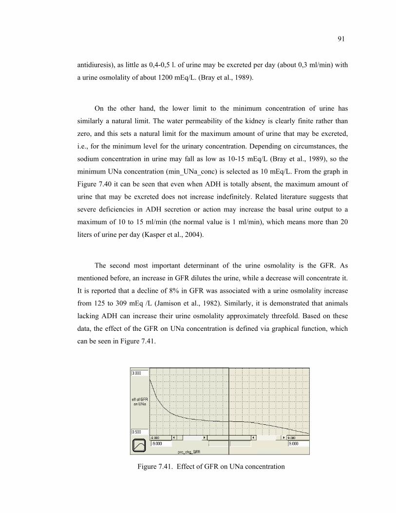
91
antidiuresis), as little as 0,4-0,5 l. of urine may be excreted per day (about 0,3 ml/min) with
a urine osmolality of about 1200 mEq/L. (Bray et al., 1989).
On the other hand, the lower limit to the minimum concentration of urine has
similarly a natural limit. The water permeability of the kidney is clearly finite rather than
zero, and this sets a natural limit for the maximum amount of urine that may be excreted,
i.e., for the minimum level for the urinary concentration. Depending on circumstances, the
sodium concentration in urine may fall as low as 10-15 mEq/L (Bray et al., 1989), so the
minimum UNa concentration (min_UNa_conc) is selected as 10 mEq/L. From the graph in
Figure 7.40 it can be seen that even when ADH is totally absent, the maximum amount of
urine that may be excreted does not increase indefinitely. Related literature suggests that
severe deficiencies in ADH secretion or action may increase the basal urine output to a
maximum of 10 to 15 ml/min (the normal value is 1 ml/min), which means more than 20
liters of urine per day (Kasper et al., 2004).
The second most important determinant of the urine osmolality is the GFR. As
mentioned before, an increase in GFR dilutes the urine, while a decrease will concentrate it.
It is reported that a decline of 8% in GFR was associated with a urine osmolality increase
from 125 to 309 mEq /L (Jamison et al., 1982). Similarly, it is demonstrated that animals
lacking ADH can increase their urine osmolality approximately threefold. Based on these
data, the effect of the GFR on UNa concentration is defined via graphical function, which
can be seen in Figure 7.41.
Figure 7.41. Effect of GFR on UNa concentration
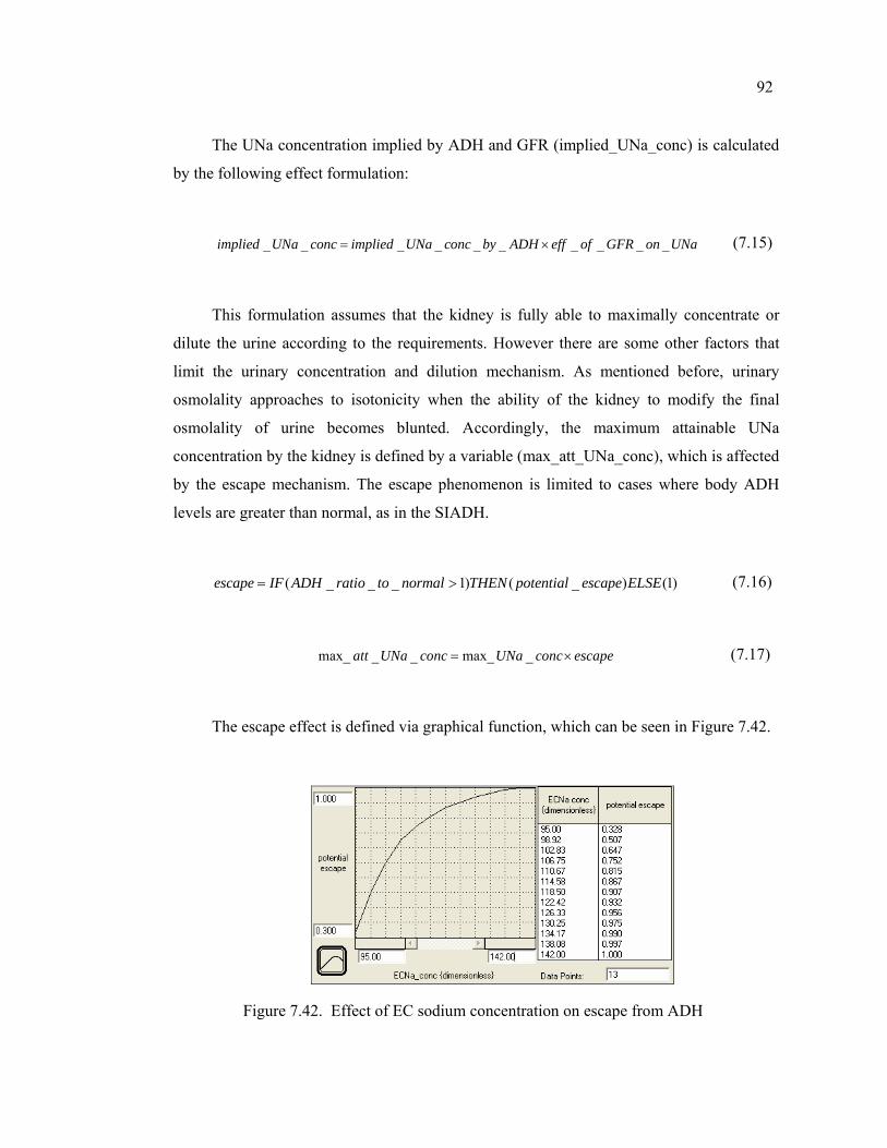
92
The UNa concentration implied by ADH and GFR (implied_UNa_conc) is calculated
by the following effect formulation:
_ _ _ _ _ _ _ _ _ _implied UNa conc implied UNa conc by ADH eff of GFR on UNa= × (7.15)
This formulation assumes that the kidney is fully able to maximally concentrate or
dilute the urine according to the requirements. However there are some other factors that
limit the urinary concentration and dilution mechanism. As mentioned before, urinary
osmolality approaches to isotonicity when the ability of the kidney to modify the final
osmolality of urine becomes blunted. Accordingly, the maximum attainable UNa
concentration by the kidney is defined by a variable (max_att_UNa_conc), which is affected
by the escape mechanism. The escape phenomenon is limited to cases where body ADH
levels are greater than normal, as in the SIADH.
( _ _ _ 1) ( _ ) (1)escape IF ADH ratio to normal THEN potential escape ELSE= > (7.16)
max_ _ _ max_ _att UNa conc UNa conc escape= × (7.17)
The escape effect is defined via graphical function, which can be seen in Figure 7.42.
Figure 7.42. Effect of EC sodium concentration on escape from ADH
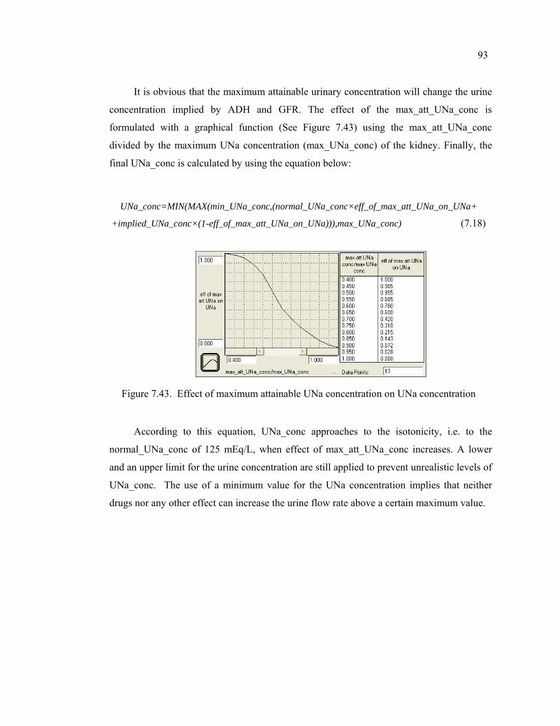
93
It is obvious that the maximum attainable urinary concentration will change the urine
concentration implied by ADH and GFR. The effect of the max_att_UNa_conc is
formulated with a graphical function (See Figure 7.43) using the max_att_UNa_conc
divided by the maximum UNa concentration (max_UNa_conc) of the kidney. Finally, the
final UNa_conc is calculated by using the equation below:
UNa_conc=MIN(MAX(min_UNa_conc,(normal_UNa_conc×eff_of_max_att_UNa_on_UNa+
+implied_UNa_conc×(1-eff_of_max_att_UNa_on_UNa))),max_UNa_conc) (7.18)
Figure 7.43. Effect of maximum attainable UNa concentration on UNa concentration
According to this equation, UNa_conc approaches to the isotonicity, i.e. to the
normal_UNa_conc of 125 mEq/L, when effect of max_att_UNa_conc increases. A lower
and an upper limit for the urine concentration are still applied to prevent unrealistic levels of
UNa_conc. The use of a minimum value for the UNa concentration implies that neither
drugs nor any other effect can increase the urine flow rate above a certain maximum value.
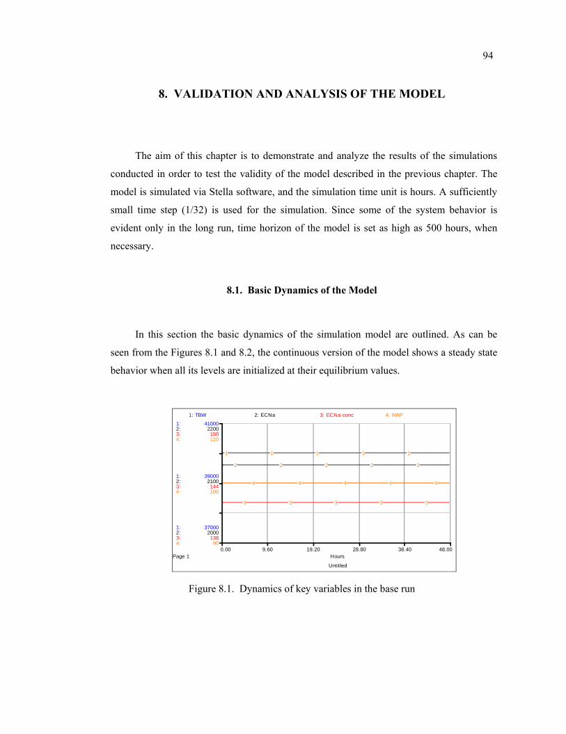
94
8. VALIDATION AND ANALYSIS OF THE MODEL
The aim of this chapter is to demonstrate and analyze the results of the simulations
conducted in order to test the validity of the model described in the previous chapter. The
model is simulated via Stella software, and the simulation time unit is hours. A sufficiently
small time step (1/32) is used for the simulation. Since some of the system behavior is
evident only in the long run, time horizon of the model is set as high as 500 hours, when
necessary.
8.1. Basic Dynamics of the Model
In this section the basic dynamics of the simulation model are outlined. As can be
seen from the Figures 8.1 and 8.2, the continuous version of the model shows a steady state
behavior when all its levels are initialized at their equilibrium values.
Untitled
Page 10.00 9.60 19.20 28.80 38.40 48.00
Hours
1:
1:
1:
2:
2:
2:
3:
3:
3:
4:
4:
4:
37000
39000
41000
2000
2100
2200
138
144
150
90
100
110
1: TBW 2: ECNa 3: ECNa conc 4: MAP
1 1 1 1 1
2 2 2 2 2
3 3 3 3 3
4 4 4 4 4
Figure 8.1. Dynamics of key variables in the base run
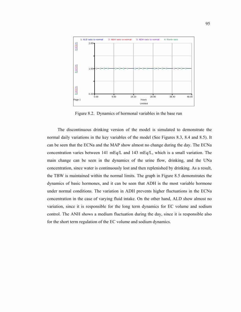
95
Untitled
Page 10.00 9.60 19.20 28.80 38.40 48.00
Hours
1:
1:
1:
2:
2:
2:
3:
3:
3:
4:
4:
4:
0.00
1.00
2.00
1: ALD ratio to normal 2: ANH ratio to normal 3: ADH ratio to normal 4: Renin ratio
1 1 1 1 12 2 2 2 23 3 3 3 34 4 4 4 4
Figure 8.2. Dynamics of hormonal variables in the base run
The discontinuous drinking version of the model is simulated to demonstrate the
normal daily variations in the key variables of the model (See Figures 8.3, 8.4 and 8.5). It
can be seen that the ECNa and the MAP show almost no change during the day. The ECNa
concentration varies between 141 mEq/L and 143 mEq/L, which is a small variation. The
main change can be seen in the dynamics of the urine flow, drinking, and the UNa
concentration, since water is continuously lost and then replenished by drinking. As a result,
the TBW is maintained within the normal limits. The graph in Figure 8.5 demonstrates the
dynamics of basic hormones, and it can be seen that ADH is the most variable hormone
under normal conditions. The variation in ADH prevents higher fluctuations in the ECNa
concentration in the case of varying fluid intake. On the other hand, ALD show almost no
variation, since it is responsible for the long term dynamics for EC volume and sodium
control. The ANH shows a medium fluctuation during the day, since it is responsible also
for the short term regulation of the EC volume and sodium dynamics.
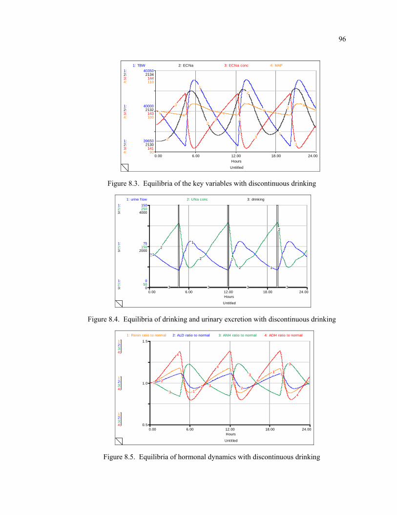
96
Untitled
0.00 6.00 12.00 18.00 24.00Hours
1:
1:
1:
2:
2:
2:
3:
3:
3:
4:
4:
4:
39650
40000
40350
2130
2132
2134
141
143
144
90
100
110
1: TBW 2: ECNa 3: ECNa conc 4: MAP
1
1
1
12
2
2
23
3
3
3
4 44
4
Figure 8.3. Equilibria of the key variables with discontinuous drinking
Untitled
0.00 6.00 12.00 18.00 24.00Hours
1:
1:
1:
2:
2:
2:
3:
3:
3:
0
75
150
50
150
250
0
2000
4000
1: urine f low 2: UNa conc 3: drinking
1
1
1
1
2
2
2
2
3 3 3 3
Figure 8.4. Equilibria of drinking and urinary excretion with discontinuous drinking
Untitled
0.00 6.00 12.00 18.00 24.00Hours
1:
1:
1:
2:
2:
2:
3:
3:
3:
4:
4:
4:
0.5
1.0
1.5
1: Renin ratio to normal 2: ALD ratio to normal 3: ANH ratio to normal 4: ADH ratio to normal
1
1
1
1
22 2
2
3
3
3
3
4
4
4
4
Figure 8.5. Equilibria of hormonal dynamics with discontinuous drinking
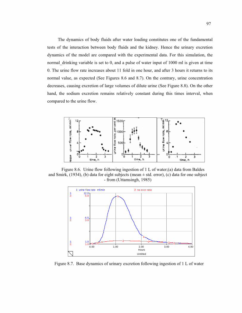
97
The dynamics of body fluids after water loading constitutes one of the fundamental
tests of the interaction between body fluids and the kidney. Hence the urinary excretion
dynamics of the model are compared with the experimental data. For this simulation, the
normal_drinking variable is set to 0, and a pulse of water input of 1000 ml is given at time
0. The urine flow rate increases about 11 fold in one hour, and after 3 hours it returns to its
normal value, as expected (See Figures 8.6 and 8.7). On the contrary, urine concentration
decreases, causing excretion of large volumes of dilute urine (See Figure 8.8). On the other
hand, the sodium excretion remains relatively constant during this times interval, when
compared to the urine flow.
Figure 8.6. Urine flow following ingestion of 1 L of water;(a) data from Baldes and Smirk, (1934), (b) data for eight subjects (mean ± std. error), (c) data for one subject
- from (Uttamsingh, 1985)
Untitled
0.00 1.00 2.00 3.00 4.00Hours
1:
1:
1:
2:
2:
2:
1.0
6.5
12.0
1.0
3.0
5.0
1: urine f low rate ml\min 2: na excr ratio
1
1
1
122 2 2
Figure 8.7. Base dynamics of urinary excretion following ingestion of 1 L of water
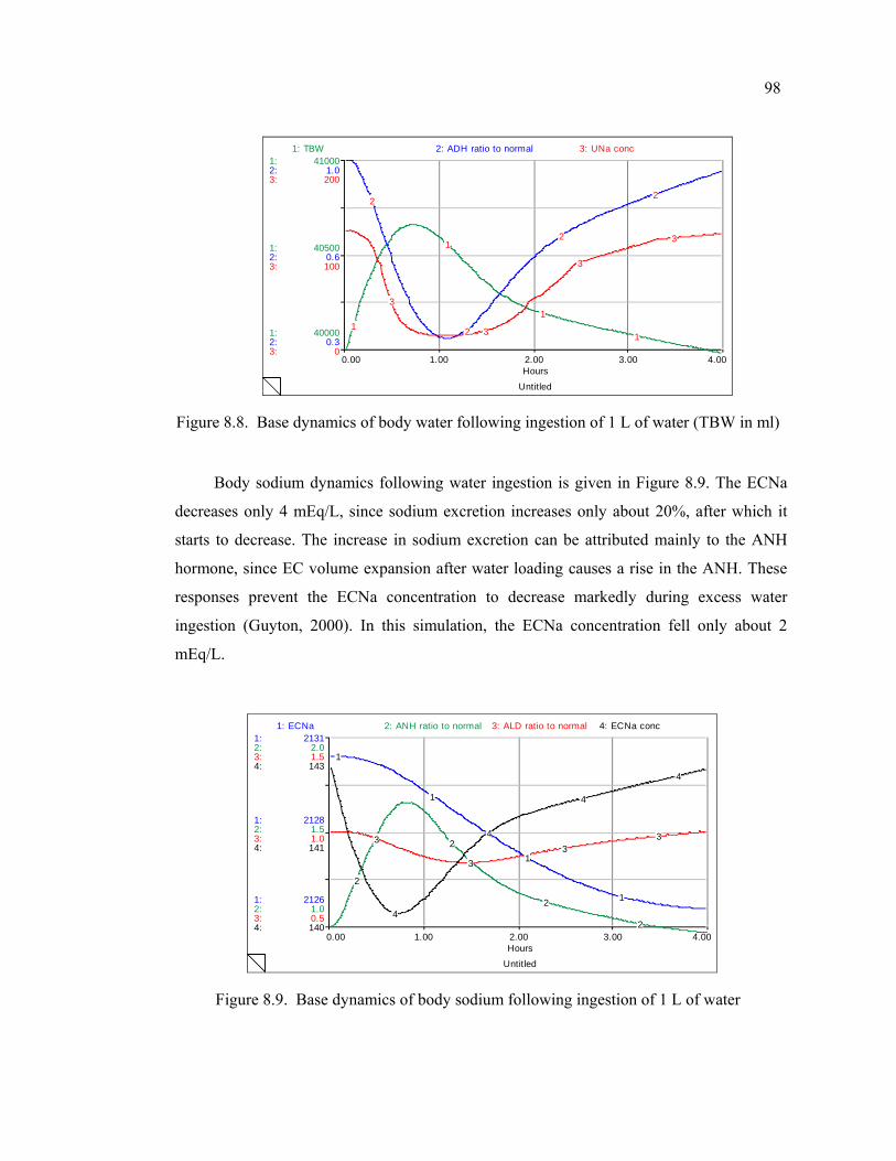
98
Untitled
0.00 1.00 2.00 3.00 4.00Hours
1:
1:
1:
2:
2:
2:
3:
3:
3:
40000
40500
41000
0.3
0.6
1.0
0
100
200
1: TBW 2: ADH ratio to normal 3: UNa conc
1
1
1
1
2
2
2
2
3
3
3
3
Figure 8.8. Base dynamics of body water following ingestion of 1 L of water (TBW in ml)
Body sodium dynamics following water ingestion is given in Figure 8.9. The ECNa
decreases only 4 mEq/L, since sodium excretion increases only about 20%, after which it
starts to decrease. The increase in sodium excretion can be attributed mainly to the ANH
hormone, since EC volume expansion after water loading causes a rise in the ANH. These
responses prevent the ECNa concentration to decrease markedly during excess water
ingestion (Guyton, 2000). In this simulation, the ECNa concentration fell only about 2
mEq/L.
Untitled
0.00 1.00 2.00 3.00 4.00Hours
1:
1:
1:
2:
2:
2:
3:
3:
3:
4:
4:
4:
2126
2128
2131
1.0
1.5
2.0
0.5
1.0
1.5
140
141
143
1: ECNa 2: ANH ratio to normal 3: ALD ratio to normal 4: ECNa conc
1
1
1
1
2
2
2
2
3
33
3
4
4
4
4
Figure 8.9. Base dynamics of body sodium following ingestion of 1 L of water
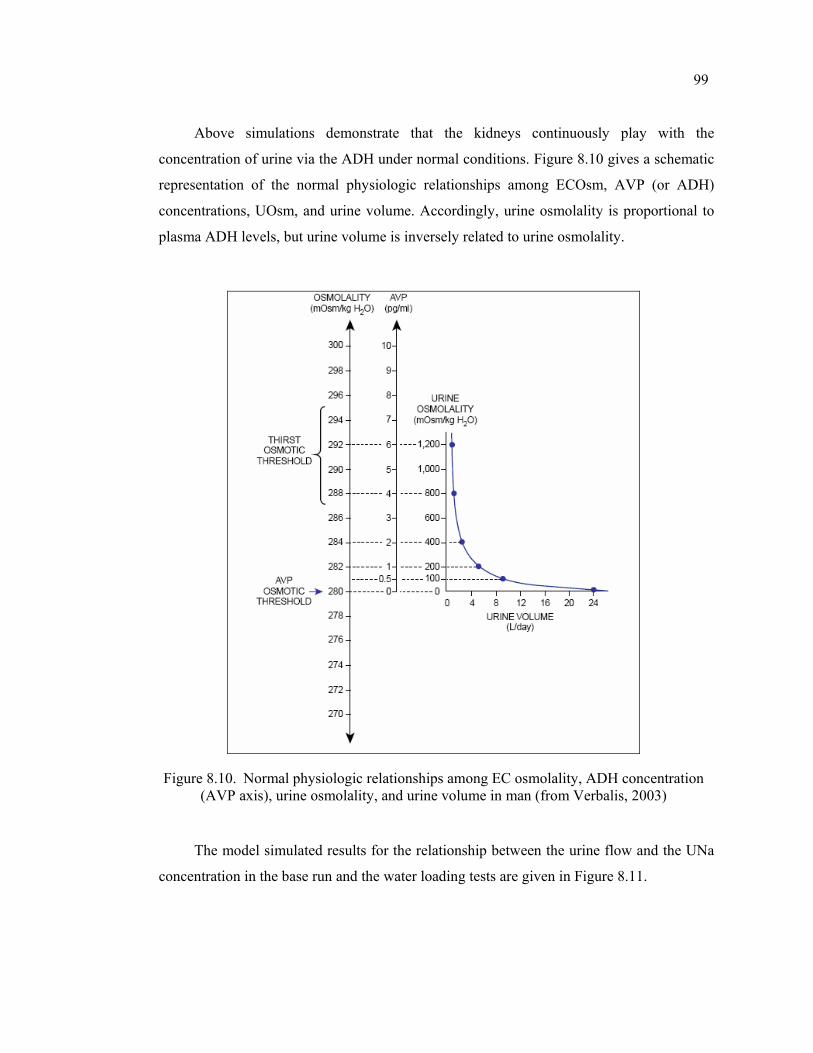
99
Above simulations demonstrate that the kidneys continuously play with the
concentration of urine via the ADH under normal conditions. Figure 8.10 gives a schematic
representation of the normal physiologic relationships among ECOsm, AVP (or ADH)
concentrations, UOsm, and urine volume. Accordingly, urine osmolality is proportional to
plasma ADH levels, but urine volume is inversely related to urine osmolality.
Figure 8.10. Normal physiologic relationships among EC osmolality, ADH concentration (AVP axis), urine osmolality, and urine volume in man (from Verbalis, 2003)
The model simulated results for the relationship between the urine flow and the UNa
concentration in the base run and the water loading tests are given in Figure 8.11.
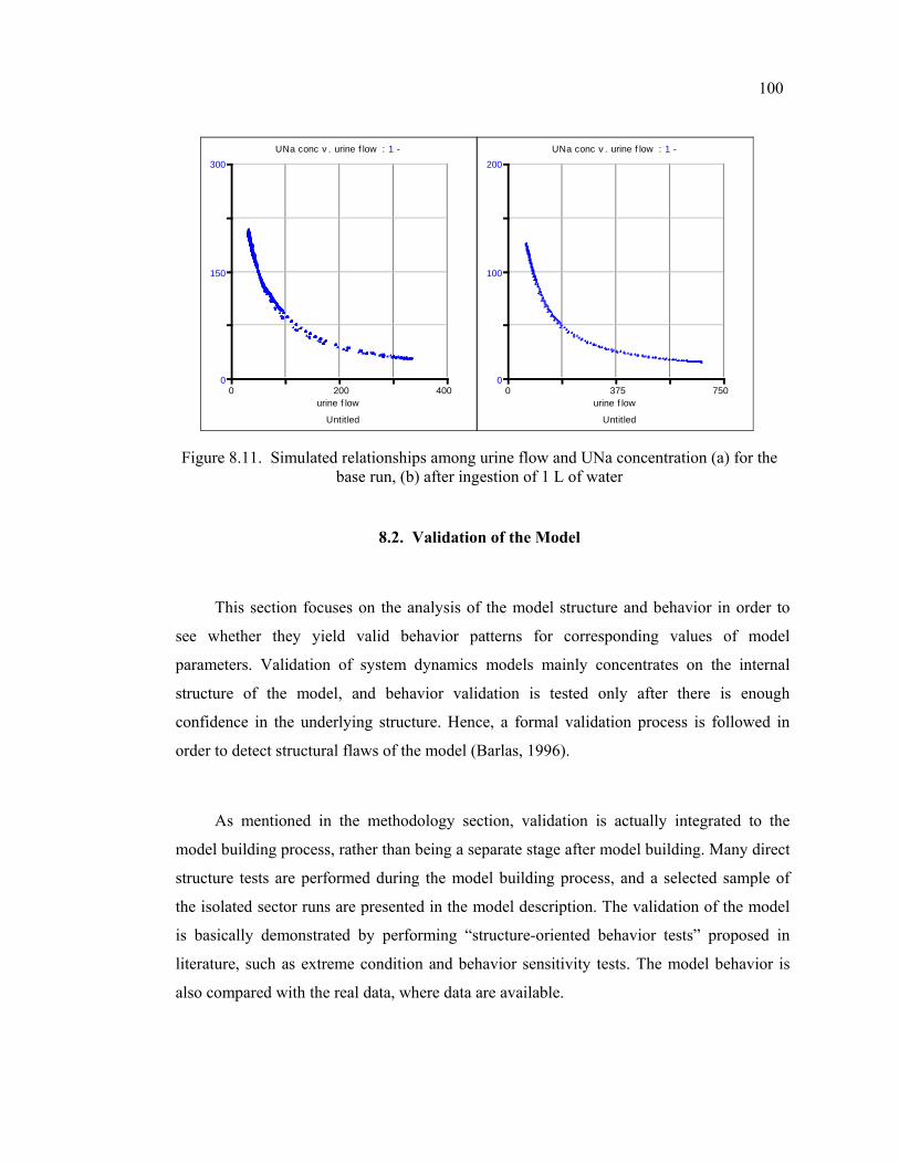
100
Untitled
urine f low 0 200 400
0
150
300UNa conc v . urine f low : 1 -
Untitled
urine f low 0 375 750
0
100
200UNa conc v . urine f low : 1 -
Figure 8.11. Simulated relationships among urine flow and UNa concentration (a) for the base run, (b) after ingestion of 1 L of water
8.2. Validation of the Model
This section focuses on the analysis of the model structure and behavior in order to
see whether they yield valid behavior patterns for corresponding values of model
parameters. Validation of system dynamics models mainly concentrates on the internal
structure of the model, and behavior validation is tested only after there is enough
confidence in the underlying structure. Hence, a formal validation process is followed in
order to detect structural flaws of the model (Barlas, 1996).
As mentioned in the methodology section, validation is actually integrated to the
model building process, rather than being a separate stage after model building. Many direct
structure tests are performed during the model building process, and a selected sample of
the isolated sector runs are presented in the model description. The validation of the model
is basically demonstrated by performing “structure-oriented behavior tests” proposed in
literature, such as extreme condition and behavior sensitivity tests. The model behavior is
also compared with the real data, where data are available.
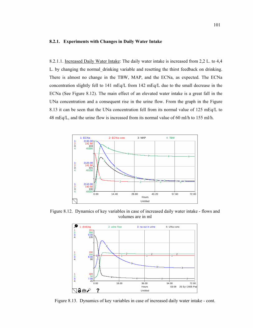
101
8.2.1. Experiments with Changes in Daily Water Intake
8.2.1.1. Increased Daily Water Intake: The daily water intake is increased from 2,2 L. to 4,4
L. by changing the normal_drinking variable and resetting the thirst feedback on drinking.
There is almost no change in the TBW, MAP, and the ECNa, as expected. The ECNa
concentration slightly fell to 141 mEq/L from 142 mEq/L due to the small decrease in the
ECNa (See Figure 8.12). The main effect of an elevated water intake is a great fall in the
UNa concentration and a consequent rise in the urine flow. From the graph in the Figure
8.13 it can be seen that the UNa concentration fell from its normal value of 125 mEq/L to
48 mEq/L, and the urine flow is increased from its normal value of 60 ml/h to 155 ml/h.
Untitled
0.00 14.40 28.80 43.20 57.60 72.00Hours
1:
1:
1:
2:
2:
2:
3:
3:
3:
4:
4:
4:
2110.00
2120.00
2130.00
140.50
141.50
142.50
100
101
103
40000
40150
40300
1: ECNa 2: ECNa conc 3: MAP 4: TBW1
1
11 1
2
2 2 2 2
3
3
3 3 3
4
44 4 4
Figure 8.12. Dynamics of key variables in case of increased daily water intake - flows and volumes are in ml
03:09 25 Ey l 2005 Paz
Untitled
0.00 18.00 36.00 54.00 72.00Hours
1:
1:
1:
2:
2:
2:
3:
3:
3:
4:
4:
4:
189
190
191
50
150
250
7.00
8.00
9.00
45
90
135
1: drinking 2: urine f low 3: na out in urine 4: UNa conc
1 1 1 12 2 2 2
3
33 3
4 4 4 4
Figure 8.13. Dynamics of key variables in case of increased daily water intake - cont.
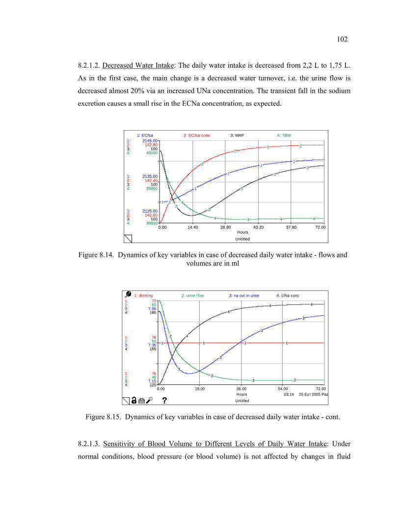
102
8.2.1.2. Decreased Water Intake: The daily water intake is decreased from 2,2 L to 1,75 L.
As in the first case, the main change is a decreased water turnover, i.e. the urine flow is
decreased almost 20% via an increased UNa concentration. The transient fall in the sodium
excretion causes a small rise in the ECNa concentration, as expected.
Untitled
0.00 14.40 28.80 43.20 57.60 72.00Hours
1:
1:
1:
2:
2:
2:
3:
3:
3:
4:
4:
4:
2125.00
2135.00
2145.00
142.00
142.40
142.80
100
100
100
39850
39950
40050
1: ECNa 2: ECNa conc 3: MAP 4: TBW
1
1
1
11
2
2
22 2
33
3
33
4
4 4 4 4
Figure 8.14. Dynamics of key variables in case of decreased daily water intake - flows and volumes are in ml
03:14 25 Ey l 2005 Paz
Untitled
0.00 18.00 36.00 54.00 72.00Hours
1:
1:
1:
2:
2:
2:
3:
3:
3:
4:
4:
4:
75
76
77
40
50
60
7.15
7.35
7.55
125
155
185
1: drinking 2: urine f low 3: na out in urine 4: UNa conc
1 1 1 1
2
22 2
3
3
3
3
4
44 4
Figure 8.15. Dynamics of key variables in case of decreased daily water intake - cont.
8.2.1.3. Sensitivity of Blood Volume to Different Levels of Daily Water Intake: Under
normal conditions, blood pressure (or blood volume) is not affected by changes in fluid
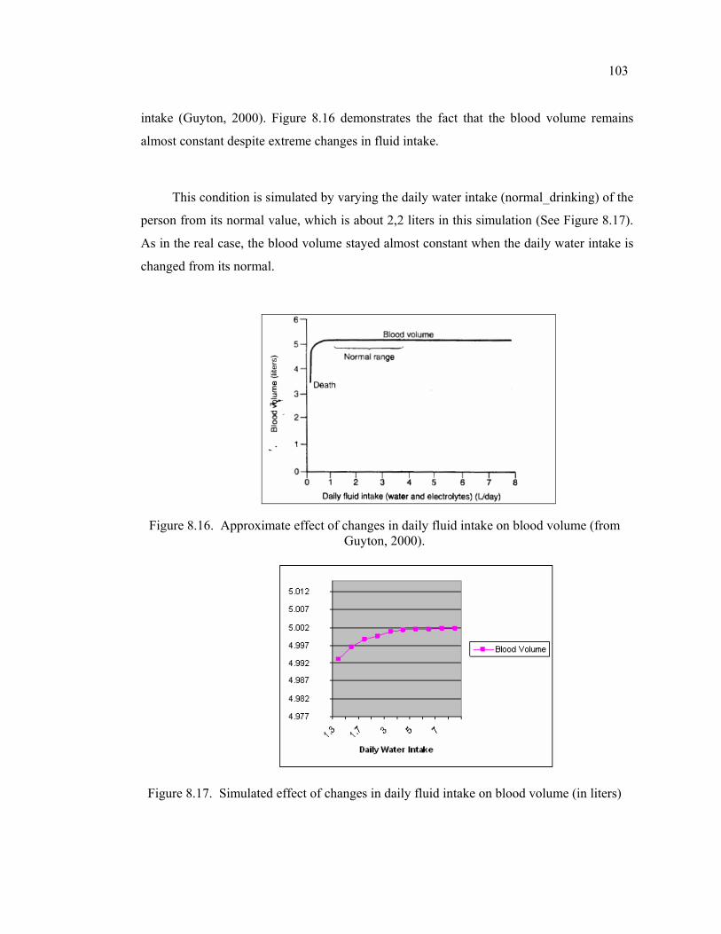
103
intake (Guyton, 2000). Figure 8.16 demonstrates the fact that the blood volume remains
almost constant despite extreme changes in fluid intake.
This condition is simulated by varying the daily water intake (normal_drinking) of the
person from its normal value, which is about 2,2 liters in this simulation (See Figure 8.17).
As in the real case, the blood volume stayed almost constant when the daily water intake is
changed from its normal.
Figure 8.16. Approximate effect of changes in daily fluid intake on blood volume (from Guyton, 2000).
Figure 8.17. Simulated effect of changes in daily fluid intake on blood volume (in liters)
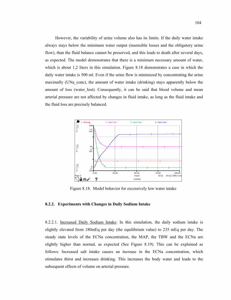
104
However, the variability of urine volume also has its limits. If the daily water intake
always stays below the minimum water output (insensible losses and the obligatory urine
flow), than the fluid balance cannot be preserved, and this leads to death after several days,
as expected. The model demonstrates that there is a minimum necessary amount of water,
which is about 1,2 liters in this simulation. Figure 8.18 demonstrates a case in which the
daily water intake is 500 ml. Even if the urine flow is minimized by concentrating the urine
maximally (UNa_conc), the amount of water intake (drinking) stays apparently below the
amount of loss (water_lost). Consequently, it can be said that blood volume and mean
arterial pressure are not affected by changes in fluid intake, as long as the fluid intake and
the fluid loss are precisely balanced.
19:21 24 Ey l 2005 Cum
Untitled
Page 30.00 25.00 50.00 75.00 100.00
Hours
1:
1:
1:
2:
2:
2:
3:
3:
3:
4:
4:
4:
0
50
100
15
40
65
100
300
500
1: drinking 2: water lost 3: urine f low 4: UNa conc
1 1 1 1
2
2 2 2
33 3 3
4
4 4 4
Figure 8.18. Model behavior for excessively low water intake
8.2.2. Experiments with Changes in Daily Sodium Intake
8.2.2.1. Increased Daily Sodium Intake: In this simulation, the daily sodium intake is
slightly elevated from 180mEq per day (the equilibrium value) to 235 mEq per day. The
steady state levels of the ECNa concentration, the MAP, the TBW and the ECNa are
slightly higher than normal, as expected (See Figure 8.19). This can be explained as
follows: Increased salt intake causes an increase in the ECNa concentration, which
stimulates thirst and increases drinking. This increases the body water and leads to the
subsequent effects of volume on arterial pressure.
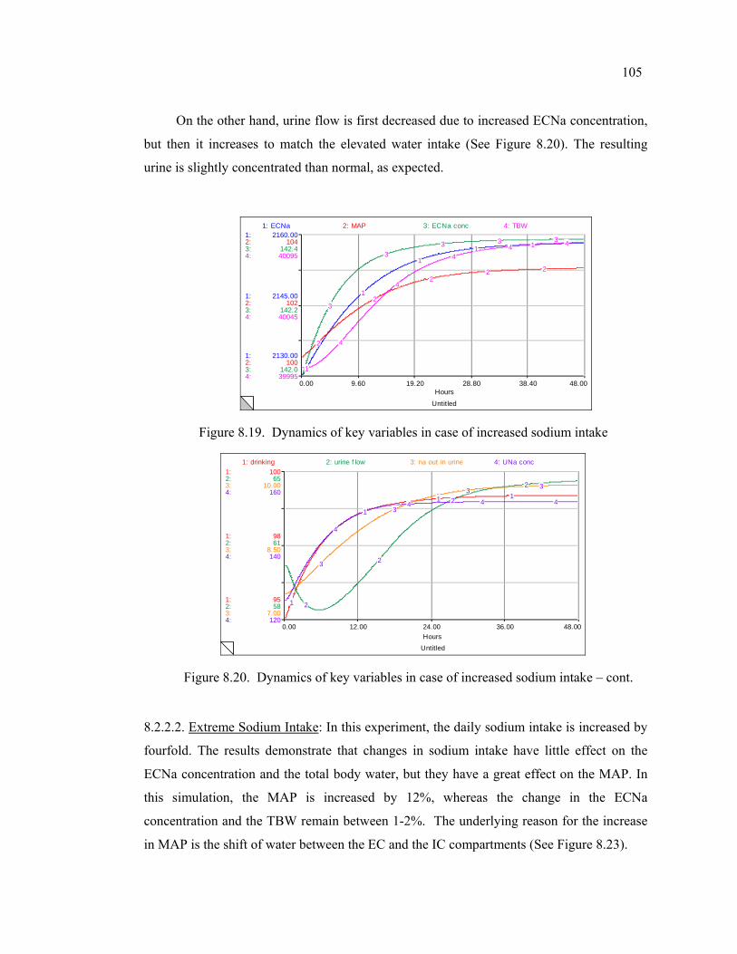
105
On the other hand, urine flow is first decreased due to increased ECNa concentration,
but then it increases to match the elevated water intake (See Figure 8.20). The resulting
urine is slightly concentrated than normal, as expected.
Untitled
0.00 9.60 19.20 28.80 38.40 48.00Hours
1:
1:
1:
2:
2:
2:
3:
3:
3:
4:
4:
4:
2130.00
2145.00
2160.00
100
102
104
142.0
142.2
142.4
39995
40045
40095
1: ECNa 2: MAP 3: ECNa conc 4: TBW
1
1
11 1
2
2
22 2
3
33 3 3
4
4
44 4
Figure 8.19. Dynamics of key variables in case of increased sodium intake
Untitled
0.00 12.00 24.00 36.00 48.00Hours
1:
1:
1:
2:
2:
2:
3:
3:
3:
4:
4:
4:
95
98
100
58
61
65
7.00
8.50
10.00
120
140
160
1: drinking 2: urine f low 3: na out in urine 4: UNa conc
1
1
1 1
2
2
2
2
3
3
33
4
4 4 4
Figure 8.20. Dynamics of key variables in case of increased sodium intake – cont.
8.2.2.2. Extreme Sodium Intake: In this experiment, the daily sodium intake is increased by
fourfold. The results demonstrate that changes in sodium intake have little effect on the
ECNa concentration and the total body water, but they have a great effect on the MAP. In
this simulation, the MAP is increased by 12%, whereas the change in the ECNa
concentration and the TBW remain between 1-2%. The underlying reason for the increase
in MAP is the shift of water between the EC and the IC compartments (See Figure 8.23).
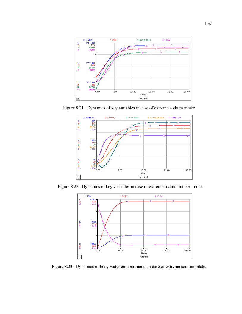
106
Untitled
0.00 7.20 14.40 21.60 28.80 36.00Hours
1:
1:
1:
2:
2:
2:
3:
3:
3:
4:
4:
4:
2100.00
2200.00
2300.00
95
105
115
142.0
144.0
146.0
39950
40100
40250
1: ECNa 2: MAP 3: ECNa conc 4: TBW
1
1
1 1 1
2
22 2 2
3
33 3 3
4
4 4 4 4
Figure 8.21. Dynamics of key variables in case of extreme sodium intake
Untitled
0.00 9.00 18.00 27.00 36.00Hours
1:
1:
1:
2:
2:
2:
3:
3:
3:
4:
4:
4:
5:
5:
5:
85
125
165
90
130
170
50
90
130
5.00
20.00
35.00
100
200
300
1: water lost 2: drinking 3: urine f low 4: na out in urine 5: UNa conc
1
1
1 1
2
22 2
3
3
3 3
4
4 4 4
5 5 5 5
Figure 8.22. Dynamics of key variables in case of extreme sodium intake – cont.
Untitled
0.00 12.00 24.00 36.00 48.00Hours
1:
1:
1:
2:
2:
2:
3:
3:
3:
40000
40500
41000
15.0
15.4
15.8
24.4
24.8
25.1
1: TBW 2: ECFV 3: ICFV
1
1 1 1
2
2 2 2
3
3 3 3
Figure 8.23. Dynamics of body water compartments in case of extreme sodium intake
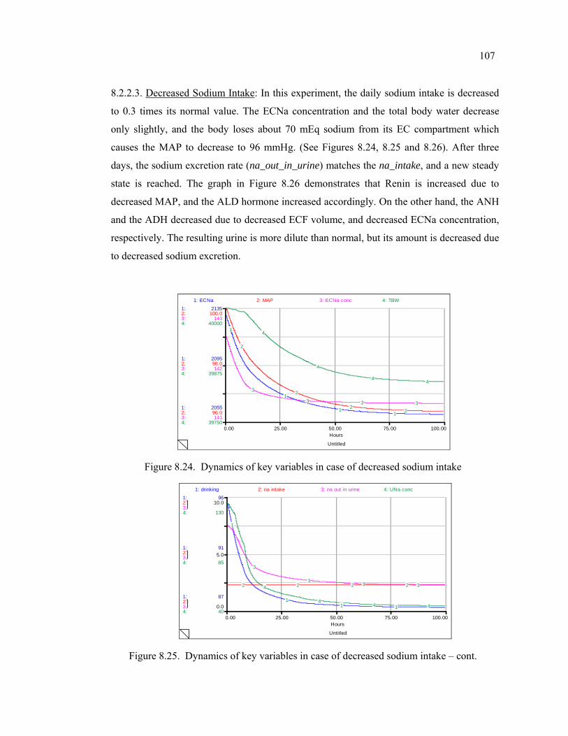
107
8.2.2.3. Decreased Sodium Intake: In this experiment, the daily sodium intake is decreased
to 0.3 times its normal value. The ECNa concentration and the total body water decrease
only slightly, and the body loses about 70 mEq sodium from its EC compartment which
causes the MAP to decrease to 96 mmHg. (See Figures 8.24, 8.25 and 8.26). After three
days, the sodium excretion rate (na_out_in_urine) matches the na_intake, and a new steady
state is reached. The graph in Figure 8.26 demonstrates that Renin is increased due to
decreased MAP, and the ALD hormone increased accordingly. On the other hand, the ANH
and the ADH decreased due to decreased ECF volume, and decreased ECNa concentration,
respectively. The resulting urine is more dilute than normal, but its amount is decreased due
to decreased sodium excretion.
Untitled
0.00 25.00 50.00 75.00 100.00Hours
1:
1:
1:
2:
2:
2:
3:
3:
3:
4:
4:
4:
2055
2095
2135
96.0
98.0
100.0
141
142
143
39750
39875
40000
1: ECNa 2: MAP 3: ECNa conc 4: TBW
1
1
11
2
2
22
3
3 3 3
4
4
4 4
Figure 8.24. Dynamics of key variables in case of decreased sodium intake
Untitled
0.00 25.00 50.00 75.00 100.00Hours
1:
1:
1:
2:
2:
2:
3:
3:
3:
4:
4:
4:
87
91
96
0.0
5.0
10.0
40
85
130
1: drinking 2: na intake 3: na out in urine 4: UNa conc
1
11 1
2 2 2 2
3
3 3 34
44 4
Figure 8.25. Dynamics of key variables in case of decreased sodium intake – cont.
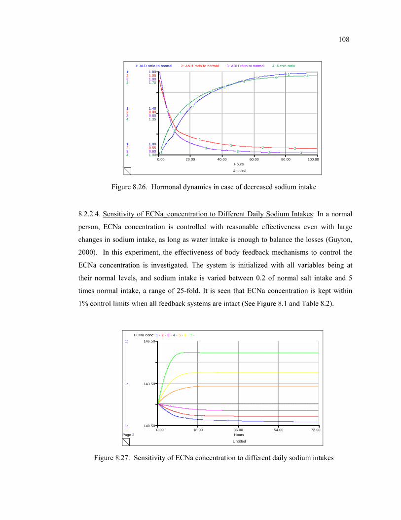
108
Untitled
0.00 20.00 40.00 60.00 80.00 100.00Hours
1:
1:
1:
2:
2:
2:
3:
3:
3:
4:
4:
4:
1.00
1.40
1.80
0.55
0.80
1.05
0.60
0.80
1.00
1.00
1.35
1.70
1: ALD ratio to normal 2: ANH ratio to normal 3: ADH ratio to normal 4: Renin ratio
1
1
1
11
2
22
2 2
3
33 3 3
4
4
44 4
Figure 8.26. Hormonal dynamics in case of decreased sodium intake
8.2.2.4. Sensitivity of ECNa_concentration to Different Daily Sodium Intakes: In a normal
person, ECNa concentration is controlled with reasonable effectiveness even with large
changes in sodium intake, as long as water intake is enough to balance the losses (Guyton,
2000). In this experiment, the effectiveness of body feedback mechanisms to control the
ECNa concentration is investigated. The system is initialized with all variables being at
their normal levels, and sodium intake is varied between 0.2 of normal salt intake and 5
times normal intake, a range of 25-fold. It is seen that ECNa concentration is kept within
1% control limits when all feedback systems are intact (See Figure 8.1 and Table 8.2).
Untitled
Page 20.00 18.00 36.00 54.00 72.00
Hours
1:
1:
1:
140.50
143.50
146.50
ECNa conc: 1 - 2 - 3 - 4 - 5 - 6 - 7 -
Figure 8.27. Sensitivity of ECNa concentration to different daily sodium intakes
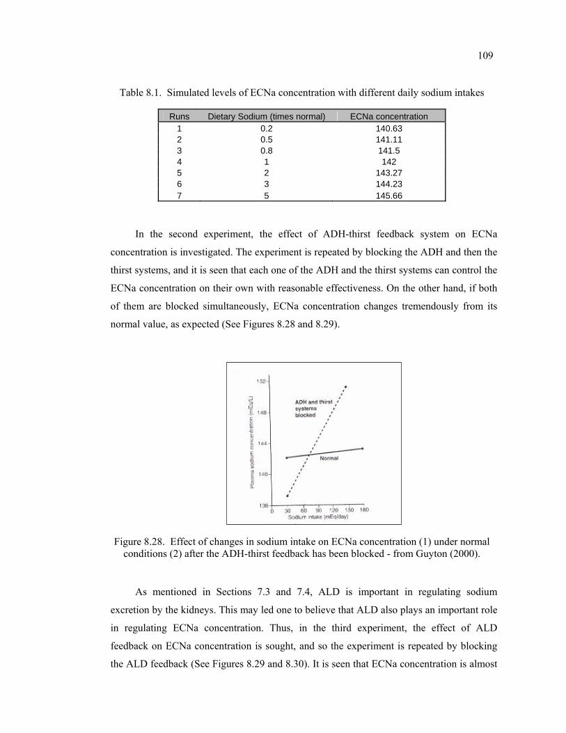
109
Table 8.1. Simulated levels of ECNa concentration with different daily sodium intakes
Runs Dietary Sodium (times normal) ECNa concentration 1 0.2 140.63 2 0.5 141.11 3 0.8 141.5 4 1 142 5 2 143.27 6 3 144.23 7 5 145.66
In the second experiment, the effect of ADH-thirst feedback system on ECNa
concentration is investigated. The experiment is repeated by blocking the ADH and then the
thirst systems, and it is seen that each one of the ADH and the thirst systems can control the
ECNa concentration on their own with reasonable effectiveness. On the other hand, if both
of them are blocked simultaneously, ECNa concentration changes tremendously from its
normal value, as expected (See Figures 8.28 and 8.29).
Figure 8.28. Effect of changes in sodium intake on ECNa concentration (1) under normal conditions (2) after the ADH-thirst feedback has been blocked - from Guyton (2000).
As mentioned in Sections 7.3 and 7.4, ALD is important in regulating sodium
excretion by the kidneys. This may led one to believe that ALD also plays an important role
in regulating ECNa concentration. Thus, in the third experiment, the effect of ALD
feedback on ECNa concentration is sought, and so the experiment is repeated by blocking
the ALD feedback (See Figures 8.29 and 8.30). It is seen that ECNa concentration is almost
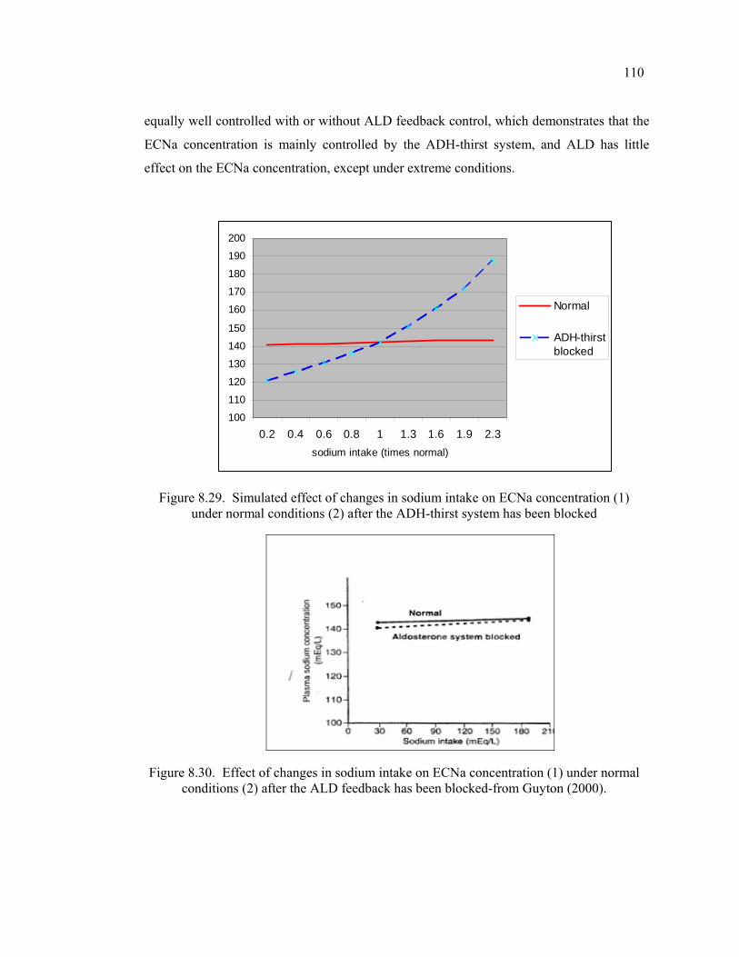
110
equally well controlled with or without ALD feedback control, which demonstrates that the
ECNa concentration is mainly controlled by the ADH-thirst system, and ALD has little
effect on the ECNa concentration, except under extreme conditions.
100
110
120
130
140
150
160
170
180
190
200
0.2 0.4 0.6 0.8 1 1.3 1.6 1.9 2.3sodium intake (times normal)
Normal
ADH-thirstblocked
Figure 8.29. Simulated effect of changes in sodium intake on ECNa concentration (1) under normal conditions (2) after the ADH-thirst system has been blocked
Figure 8.30. Effect of changes in sodium intake on ECNa concentration (1) under normal conditions (2) after the ALD feedback has been blocked-from Guyton (2000).
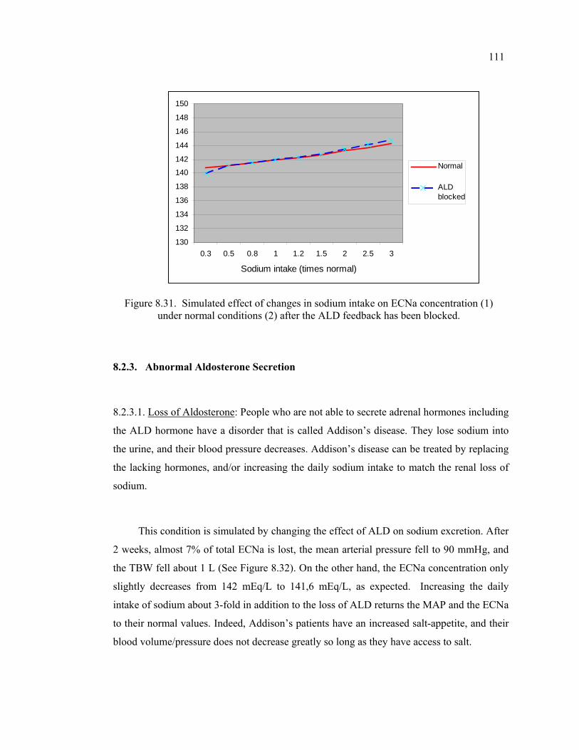
111
130
132
134
136
138
140
142
144
146
148
150
0.3 0.5 0.8 1 1.2 1.5 2 2.5 3
Sodium intake (times normal)
Normal
ALDblocked
Figure 8.31. Simulated effect of changes in sodium intake on ECNa concentration (1) under normal conditions (2) after the ALD feedback has been blocked.
8.2.3. Abnormal Aldosterone Secretion
8.2.3.1. Loss of Aldosterone: People who are not able to secrete adrenal hormones including
the ALD hormone have a disorder that is called Addison’s disease. They lose sodium into
the urine, and their blood pressure decreases. Addison’s disease can be treated by replacing
the lacking hormones, and/or increasing the daily sodium intake to match the renal loss of
sodium.
This condition is simulated by changing the effect of ALD on sodium excretion. After
2 weeks, almost 7% of total ECNa is lost, the mean arterial pressure fell to 90 mmHg, and
the TBW fell about 1 L (See Figure 8.32). On the other hand, the ECNa concentration only
slightly decreases from 142 mEq/L to 141,6 mEq/L, as expected. Increasing the daily
intake of sodium about 3-fold in addition to the loss of ALD returns the MAP and the ECNa
to their normal values. Indeed, Addison’s patients have an increased salt-appetite, and their
blood volume/pressure does not decrease greatly so long as they have access to salt.
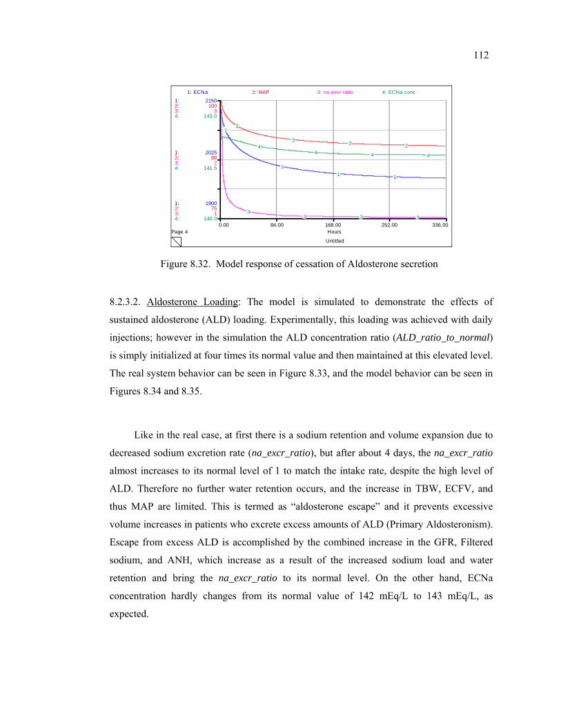
112
Untitled
Page 40.00 84.00 168.00 252.00 336.00
Hours
1:
1:
1:
2:
2:
2:
3:
3:
3:
4:
4:
4:
1900
2025
2150
75
88
100
1
2
3
140.0
141.5
143.0
1: ECNa 2: MAP 3: na excr ratio 4: ECNa conc
1
11 1
2
22 2
33 3 3
44 4 4
Figure 8.32. Model response of cessation of Aldosterone secretion
8.2.3.2. Aldosterone Loading: The model is simulated to demonstrate the effects of
sustained aldosterone (ALD) loading. Experimentally, this loading was achieved with daily
injections; however in the simulation the ALD concentration ratio (ALD_ratio_to_normal)
is simply initialized at four times its normal value and then maintained at this elevated level.
The real system behavior can be seen in Figure 8.33, and the model behavior can be seen in
Figures 8.34 and 8.35.
Like in the real case, at first there is a sodium retention and volume expansion due to
decreased sodium excretion rate (na_excr_ratio), but after about 4 days, the na_excr_ratio
almost increases to its normal level of 1 to match the intake rate, despite the high level of
ALD. Therefore no further water retention occurs, and the increase in TBW, ECFV, and
thus MAP are limited. This is termed as “aldosterone escape” and it prevents excessive
volume increases in patients who excrete excess amounts of ALD (Primary Aldosteronism).
Escape from excess ALD is accomplished by the combined increase in the GFR, Filtered
sodium, and ANH, which increase as a result of the increased sodium load and water
retention and bring the na_excr_ratio to its normal level. On the other hand, ECNa
concentration hardly changes from its normal value of 142 mEq/L to 143 mEq/L, as
expected.
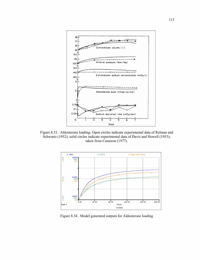
113
Figure 8.33. Aldosterone loading: Open circles indicate experimental data of Relman and Schwartz (1952); solid circles indicate experimental data of Davis and Howell (1953);
taken from Cameron (1977).
Untitled
Page 10.00 40.00 80.00 120.00 160.00 200.00
Hours
1:
1:
1:
2:
2:
2:
3:
3:
3:
40000
41000
42000
15.0
16.5
18.0
100
120
140
1: TBW 2: ECFV 3: Mean Arter Press
1
1
11
1
2
2
22 2
3
3
33 3
Figure 8.34. Model generated outputs for Aldosterone loading
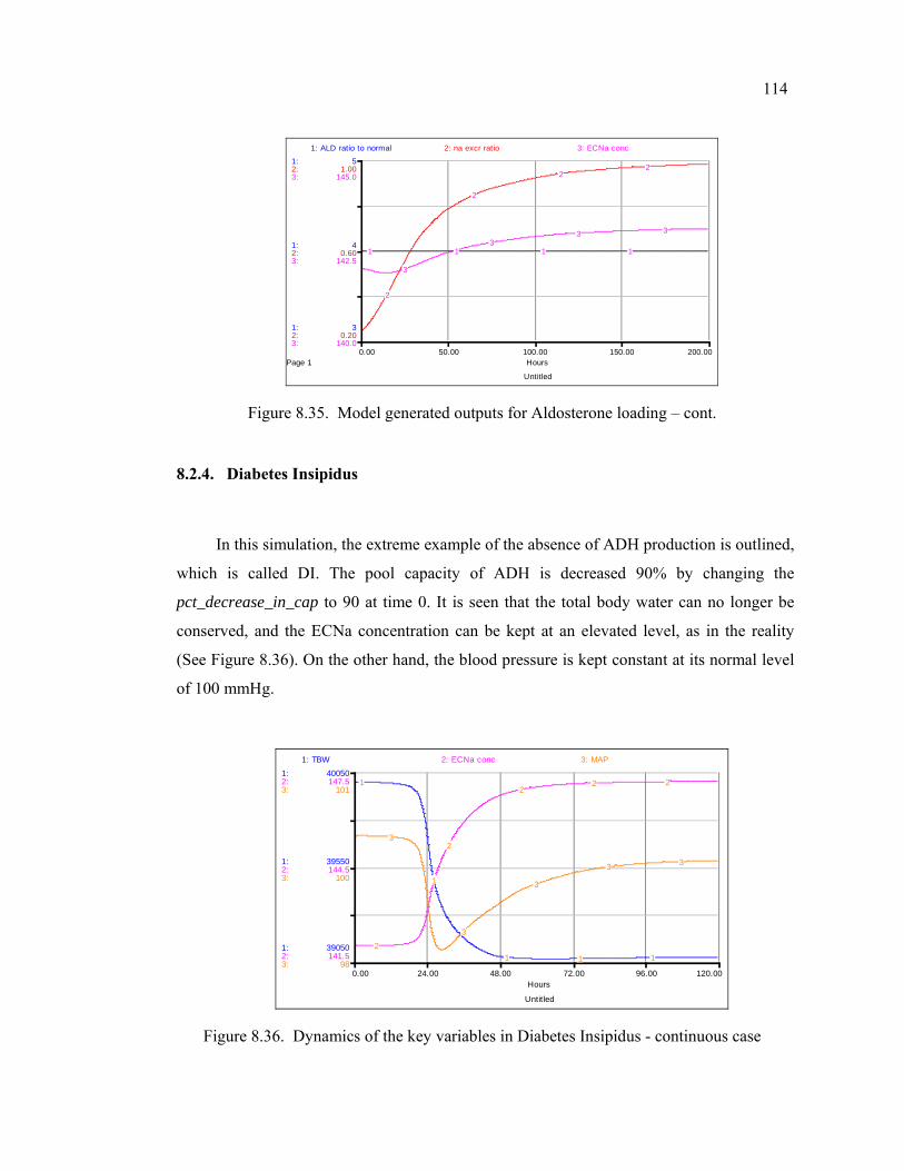
114
Untitled
Page 10.00 50.00 100.00 150.00 200.00
Hours
1:
1:
1:
2:
2:
2:
3:
3:
3:
3
4
5
0.20
0.60
1.00
140.0
142.5
145.0
1: ALD ratio to normal 2: na excr ratio 3: ECNa conc
1 1 1 1
2
2
22
3
33 3
Figure 8.35. Model generated outputs for Aldosterone loading – cont.
8.2.4. Diabetes Insipidus
In this simulation, the extreme example of the absence of ADH production is outlined,
which is called DI. The pool capacity of ADH is decreased 90% by changing the
pct_decrease_in_cap to 90 at time 0. It is seen that the total body water can no longer be
conserved, and the ECNa concentration can be kept at an elevated level, as in the reality
(See Figure 8.36). On the other hand, the blood pressure is kept constant at its normal level
of 100 mmHg.
Untitled
0.00 24.00 48.00 72.00 96.00 120.00Hours
1:
1:
1:
2:
2:
2:
3:
3:
3:
39050
39550
40050
141.5
144.5
147.5
98
100
101
1: TBW 2: ECNa conc 3: MAP
1
1
1 1 12
2
22 2
3
3
3
3 3
Figure 8.36. Dynamics of the key variables in Diabetes Insipidus - continuous case
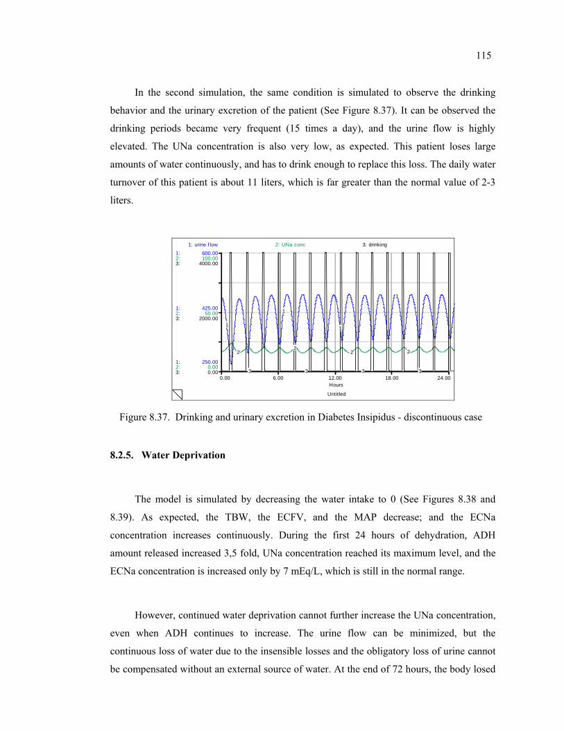
115
In the second simulation, the same condition is simulated to observe the drinking
behavior and the urinary excretion of the patient (See Figure 8.37). It can be observed the
drinking periods became very frequent (15 times a day), and the urine flow is highly
elevated. The UNa concentration is also very low, as expected. This patient loses large
amounts of water continuously, and has to drink enough to replace this loss. The daily water
turnover of this patient is about 11 liters, which is far greater than the normal value of 2-3
liters.
Untitled
0.00 6.00 12.00 18.00 24.00Hours
1:
1:
1:
2:
2:
2:
3:
3:
3:
250.00
425.00
600.00
0.00
50.00
100.00
0.00
2000.00
4000.00
1: urine f low 2: UNa conc 3: drinking
1
1
1
1
22
2 2
3 3 3 3
Figure 8.37. Drinking and urinary excretion in Diabetes Insipidus - discontinuous case
8.2.5. Water Deprivation
The model is simulated by decreasing the water intake to 0 (See Figures 8.38 and
8.39). As expected, the TBW, the ECFV, and the MAP decrease; and the ECNa
concentration increases continuously. During the first 24 hours of dehydration, ADH
amount released increased 3,5 fold, UNa concentration reached its maximum level, and the
ECNa concentration is increased only by 7 mEq/L, which is still in the normal range.
However, continued water deprivation cannot further increase the UNa concentration,
even when ADH continues to increase. The urine flow can be minimized, but the
continuous loss of water due to the insensible losses and the obligatory loss of urine cannot
be compensated without an external source of water. At the end of 72 hours, the body losed
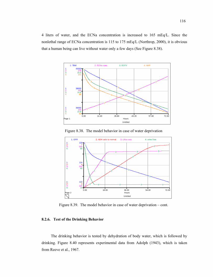
116
4 liters of water, and the ECNa concentration is increased to 165 mEq/L. Since the
nonlethal range of ECNa concentration is 115 to 175 mEq/L (Northrop, 2000), it is obvious
that a human being can live without water only a few days (See Figure 8.38).
Untitled
Page 10.00 14.40 28.80 43.20 57.60 72.00
Hours
1:
1:
1:
2:
2:
2:
3:
3:
3:
4:
4:
4:
36000
38000
40000
140
155
170
14.5
14.8
15.0
96
98
101
1: TBW 2: ECNa conc 3: ECFV 4: MAP
1
1
1
1
1
2
2
2
2
23
3
3
3
3
4
4
4
4
4
Figure 8.38. The model behavior in case of water deprivation
Untitled
Page 20.00 18.00 36.00 54.00 72.00
Hours
1:
1:
1:
2:
2:
2:
3:
3:
3:
4:
4:
4:
122
124
125
1
4
7
125
313
500
15
40
65
1: GFR 2: ADH ratio to normal 3: UNa conc 4: urine f low
1
1
1
1
2
2
2
2
3
3 3 3
4 4 4 4
Figure 8.39. The model behavior in case of water deprivation – cont.
8.2.6. Test of the Drinking Behavior
The drinking behavior is tested by dehydration of body water, which is followed by
drinking. Figure 8.40 represents experimental data from Adolph (1943), which is taken
from Reeve et al., 1967.
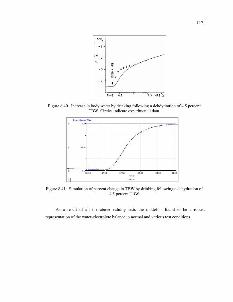
117
Figure 8.40. Increase in body water by drinking following a dehdydration of 4.5 percent TBW. Circles indicate experimental data.
Untitled
31.50 32.00 32.50 33.00 33.50 34.00Hours
1:
1:
1:
-4.5
-2.3
0.0
1: pct change TBW
1 1
1
1
1
Figure 8.41. Simulation of percent change in TBW by drinking following a dehydration of 4.5 percent TBW
As a result of all the above validity tests the model is found to be a robust
representation of the water-electrolyte balance in normal and various test conditions.
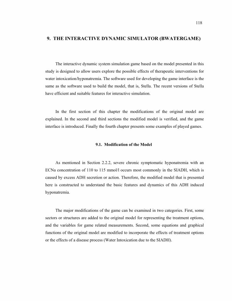
118
9. THE INTERACTIVE DYNAMIC SIMULATOR (BWATERGAME)
The interactive dynamic system simulation game based on the model presented in this
study is designed to allow users explore the possible effects of therapeutic interventions for
water intoxication/hyponatremia. The software used for developing the game interface is the
same as the software used to build the model, that is, Stella. The recent versions of Stella
have efficient and suitable features for interactive simulation.
In the first section of this chapter the modifications of the original model are
explained. In the second and third sections the modified model is verified, and the game
interface is introduced. Finally the fourth chapter presents some examples of played games.
9.1. Modification of the Model
As mentioned in Section 2.2.2, severe chronic symptomatic hyponatremia with an
ECNa concentration of 110 to 115 mmol/l occurs most commonly in the SIADH, which is
caused by excess ADH secretion or action. Therefore, the modified model that is presented
here is constructed to understand the basic features and dynamics of this ADH induced
hyponatremia.
The major modifications of the game can be examined in two categories. First, some
sectors or structures are added to the original model for representing the treatment options,
and the variables for game related measurements. Second, some equations and graphical
functions of the original model are modified to incorporate the effects of treatment options
or the effects of a disease process (Water Intoxication due to the SIADH).
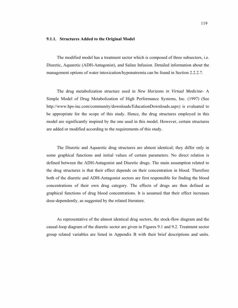
119
9.1.1. Structures Added to the Original Model
The modified model has a treatment sector which is composed of three subsectors, i.e.
Diuretic, Aquaretic (ADH-Antagonist), and Saline Infusion. Detailed information about the
management options of water intoxication/hyponatremia can be found in Section 2.2.2.7.
The drug metabolization structure used in New Horizons in Virtual Medicine- A
Simple Model of Drug Metabolization of High Performance Systems, Inc. (1997) (See
http://www.hps-inc.com/community/downloads/EducationDownloads.aspx) is evaluated to
be appropriate for the scope of this study. Hence, the drug structures employed in this
model are significantly inspired by the one used in this model. However, certain structures
are added or modified according to the requirements of this study.
The Diuretic and Aquaretic drug structures are almost identical; they differ only in
some graphical functions and initial values of certain parameters. No direct relation is
defined between the ADH-Antagonist and Diuretic drugs. The main assumption related to
the drug structures is that their effect depends on their concentration in blood. Therefore
both of the diuretic and ADH-Antagonist sectors are first responsible for finding the blood
concentrations of their own drug category. The effects of drugs are then defined as
graphical functions of drug blood concentrations. It is assumed that their effect increases
dose-dependently, as suggested by the related literature.
As representative of the almost identical drug sectors, the stock-flow diagram and the
causal-loop diagram of the diuretic sector are given in Figures 9.1 and 9.2. Treatment sector
group related variables are listed in Appendix B with their brief descriptions and units.
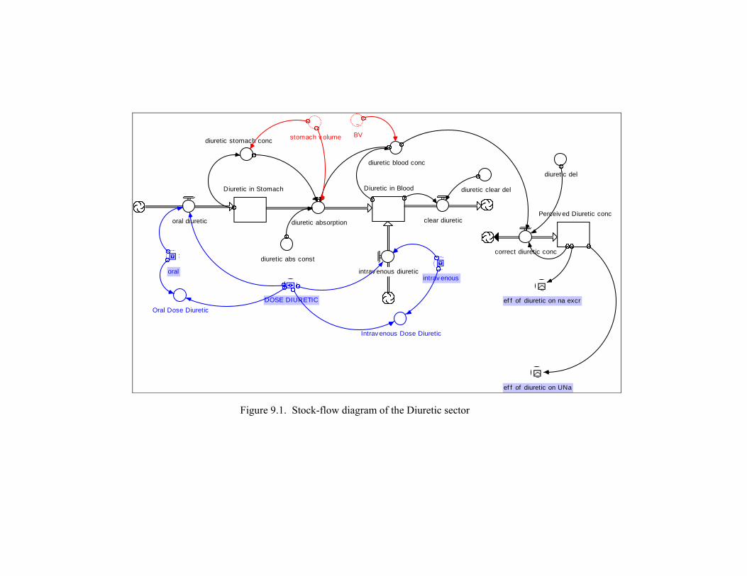
~ef f of diuretic on na excr
Diuretic in Blood
intrav enous diuretic
clear diuretic
diuretic clear del
diuretic blood conc
diuretic absorptionPerceiv ed Diuretic conc
correct diuretic conc
diuretic del
DOSE DIURETIC
~ef f of diuretic on UNa
Diuretic in Stomach
oral diuretic
diuretic abs const
stomach v olume
oral
diuretic stomach conc
intrav enous
~BV
Oral Dose Diuretic
Intrav enous Dose Diuretic
Figure 9.1. Stock-flow diagram of the Diuretic sector
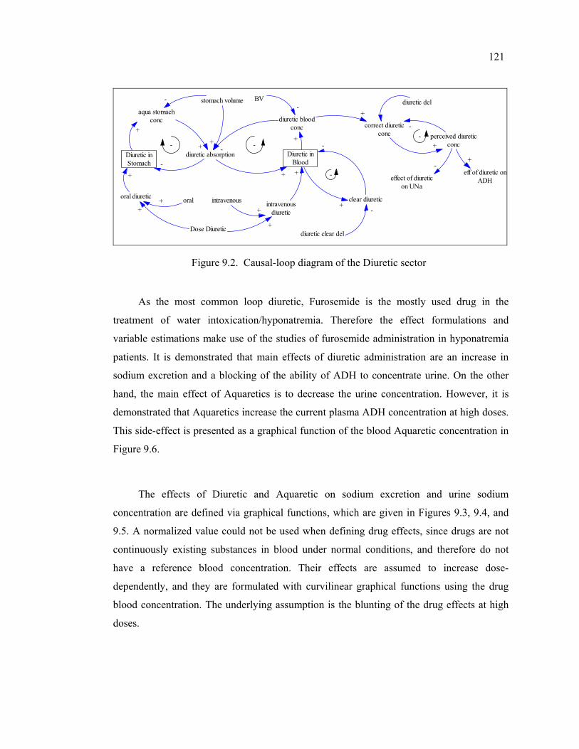
121
Diuretic inStomach
diuretic absorption Diuretic inBlood
oral diuretic
aqua stomachconc
stomach volume
diuretic bloodconc
BV
clear diuretic
diuretic clear del
perceived diureticconc
effect of diureticon UNa
intravenousdiuretic
Dose Diuretic
oral intravenous
diuretic del
correct diureticconc
+
-
++ -
-
+
-+
- -
+ +
+
-
-
+
+
-
-
+
+
++
-
eff of diuretic onADH
+
-
Figure 9.2. Causal-loop diagram of the Diuretic sector
As the most common loop diuretic, Furosemide is the mostly used drug in the
treatment of water intoxication/hyponatremia. Therefore the effect formulations and
variable estimations make use of the studies of furosemide administration in hyponatremia
patients. It is demonstrated that main effects of diuretic administration are an increase in
sodium excretion and a blocking of the ability of ADH to concentrate urine. On the other
hand, the main effect of Aquaretics is to decrease the urine concentration. However, it is
demonstrated that Aquaretics increase the current plasma ADH concentration at high doses.
This side-effect is presented as a graphical function of the blood Aquaretic concentration in
Figure 9.6.
The effects of Diuretic and Aquaretic on sodium excretion and urine sodium
concentration are defined via graphical functions, which are given in Figures 9.3, 9.4, and
9.5. A normalized value could not be used when defining drug effects, since drugs are not
continuously existing substances in blood under normal conditions, and therefore do not
have a reference blood concentration. Their effects are assumed to increase dose-
dependently, and they are formulated with curvilinear graphical functions using the drug
blood concentration. The underlying assumption is the blunting of the drug effects at high
doses.
122
Figure 9.3. Effect of Diuretic on sodium excretion
Figure 9.4. Effect of Diuretic on UNa concentration
Figure 9.5. Effect of Aquaretic on UNa concentration
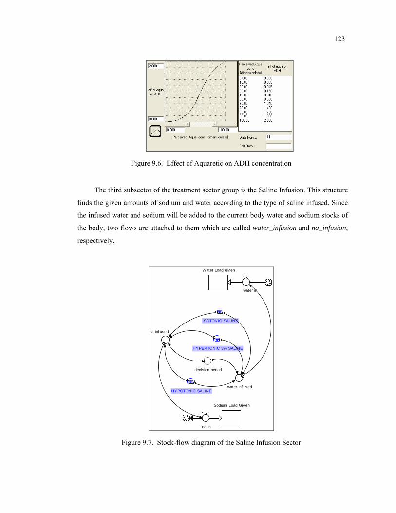
123
Figure 9.6. Effect of Aquaretic on ADH concentration
The third subsector of the treatment sector group is the Saline Infusion. This structure
finds the given amounts of sodium and water according to the type of saline infused. Since
the infused water and sodium will be added to the current body water and sodium stocks of
the body, two flows are attached to them which are called water_infusion and na_infusion,
respectively.
water in
Sodium Load Giv en
na in
Water Load giv en
decision period
ISOTONIC SALINE
HYPERTONIC 3% SALINE
na inf used
water inf usedHYPOTONIC SALINE
Figure 9.7. Stock-flow diagram of the Saline Infusion Sector
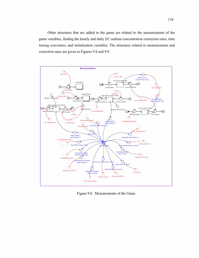
124
Other structures that are added to the game are related to the measurements of the
game variables, finding the hourly and daily EC sodium concentration correction rates, time
tracing converters, and initialization variables. The structures related to measurements and
correction rates are given in Figures 9.8 and 9.9.
Urinary Na conc
Urinary Na Concentration \ mEq\L
urine f low
decision period
water intake rate
drinking
Water Intake Current Period
na out in urine
Water Intake in current Period \ L
ExtracellularNa conc
ANH ratio to normal
ALD ratio to normal
Extracellular Na \ mEq
na intake plus inf usionExtracellular Fluid Vol
Intracellular Fluid Vol
~Mean Arter Press
~Glomerular Filtr Rate
Renin ratio
ADH ratio to normal
decision periodExtracellular Sodium \ mEq
Body Water \ L
Extracellular Fluid Volume \ L
Intracellular Fluid Volume \ L
Mean Arterial Pressure \ mmHg
Glomerular Filtration Rate \ ml\minExtracellular Sodium
Concentration\ mEq\L
na intake period
Na In Current Period
Atrial Natriuretic Hormone Ratio to normal
Renin Ratio to normal
Aldosterone Ratio to normalAntidiuretic Hormone
Ratio to normal
Total Body Water
Urine Output in current Period \ L
Sodium Lost in Current Period \ mEq
Sodium Intake in current Period \ mEq
water inf used
water in periodwater out period
Na Out Current Period
na lost period
Urine Output Current Period
UFlow in period
dec v ariable period
UFlow out period
dec v ariable period
WaterInPeriod
f luid intake
decision period
Urine Period
urine f low
urine f low
na out period
na lost out period
dec v ariable periodWaterIn current period
UrineOut current period
Measurements
Figure 9.8. Measurements of the Game
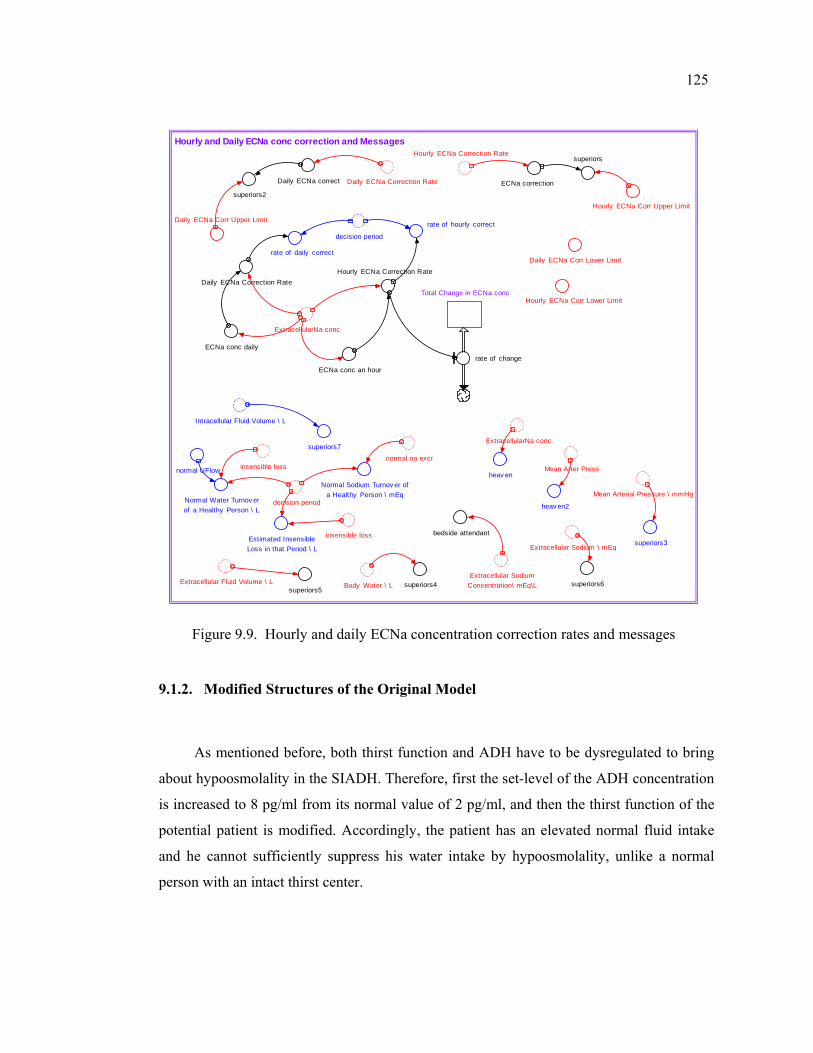
125
normal UFlow
Hourly ECNa Correction Rate
Daily ECNa Correction Rate
Daily ECNa Corr Lower Limit
rate of hourly correct
decision period
rate of daily correct
ExtracellularNa conc
Hourly ECNa Correction Rate
superiors3
ExtracellularNa conc
ECNa conc daily
ECNa conc an hour
Daily ECNa Correction RateTotal Change in ECNa conc
rate of change
Hourly ECNa Corr Upper Limit
Daily ECNa Corr Upper Limit
superiors4
Hourly ECNa Corr Lower Limit
heav en
superiors5
~Mean Arter Press
ECNa correction
superiors
Daily ECNa correct
superiors2
bedside attendant
heav en2
Extracellular Sodium Concentration\ mEq\L
insensible loss
Extracellular Sodium \ mEq
Mean Arterial Pressure \ mmHg
Body Water \ LExtracellular Fluid Volume \ L superiors6
decision periodNormal Water Turnov er of a Healthy Person \ L
Normal Sodium Turnov er of a Healthy Person \ mEq
normal na excr
insensible lossEstimated Insensible Loss in that Period \ L
Intracellular Fluid Volume \ L
superiors7
Hourly and Daily ECNa conc correction and Messages
Figure 9.9. Hourly and daily ECNa concentration correction rates and messages
9.1.2. Modified Structures of the Original Model
As mentioned before, both thirst function and ADH have to be dysregulated to bring
about hypoosmolality in the SIADH. Therefore, first the set-level of the ADH concentration
is increased to 8 pg/ml from its normal value of 2 pg/ml, and then the thirst function of the
potential patient is modified. Accordingly, the patient has an elevated normal fluid intake
and he cannot sufficiently suppress his water intake by hypoosmolality, unlike a normal
person with an intact thirst center.
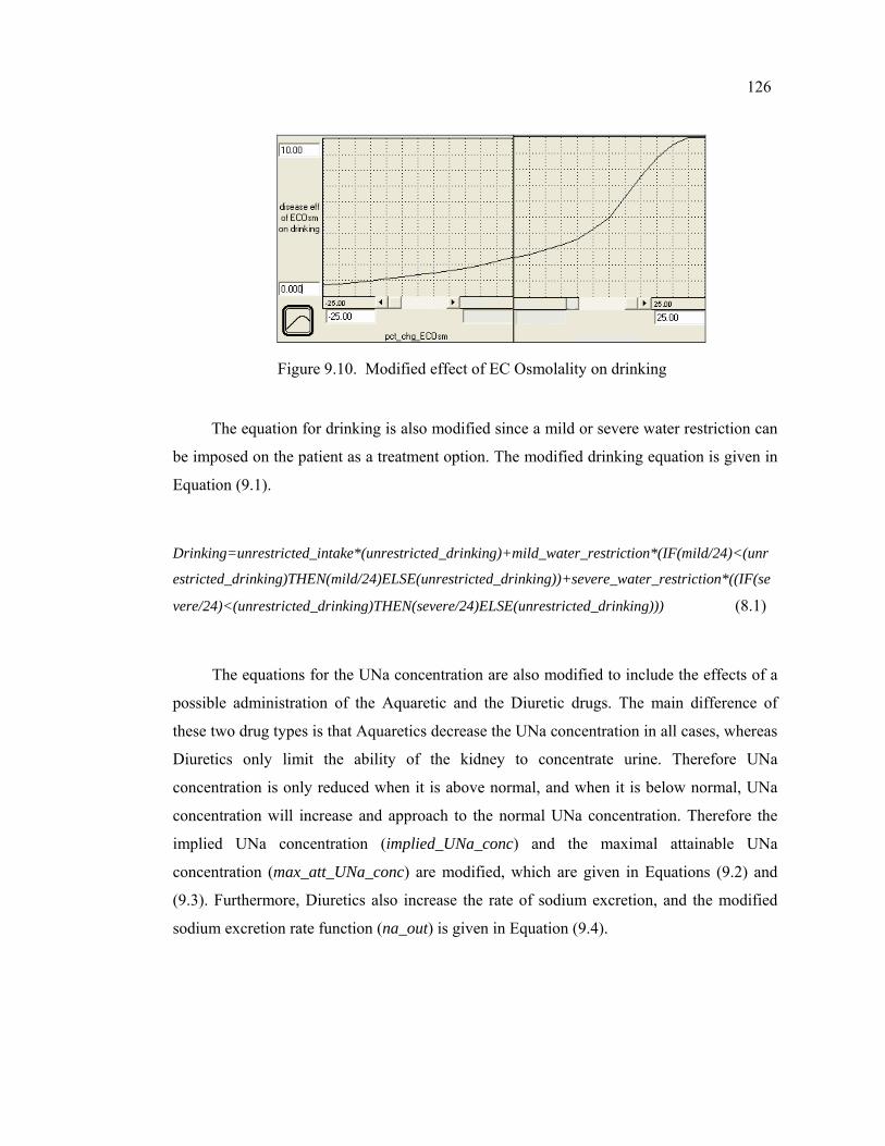
126
Figure 9.10. Modified effect of EC Osmolality on drinking
The equation for drinking is also modified since a mild or severe water restriction can
be imposed on the patient as a treatment option. The modified drinking equation is given in
Equation (9.1).
Drinking=unrestricted_intake*(unrestricted_drinking)+mild_water_restriction*(IF(mild/24)<(unr
estricted_drinking)THEN(mild/24)ELSE(unrestricted_drinking))+severe_water_restriction*((IF(se
vere/24)<(unrestricted_drinking)THEN(severe/24)ELSE(unrestricted_drinking))) (8.1)
The equations for the UNa concentration are also modified to include the effects of a
possible administration of the Aquaretic and the Diuretic drugs. The main difference of
these two drug types is that Aquaretics decrease the UNa concentration in all cases, whereas
Diuretics only limit the ability of the kidney to concentrate urine. Therefore UNa
concentration is only reduced when it is above normal, and when it is below normal, UNa
concentration will increase and approach to the normal UNa concentration. Therefore the
implied UNa concentration (implied_UNa_conc) and the maximal attainable UNa
concentration (max_att_UNa_conc) are modified, which are given in Equations (9.2) and
(9.3). Furthermore, Diuretics also increase the rate of sodium excretion, and the modified
sodium excretion rate function (na_out) is given in Equation (9.4).
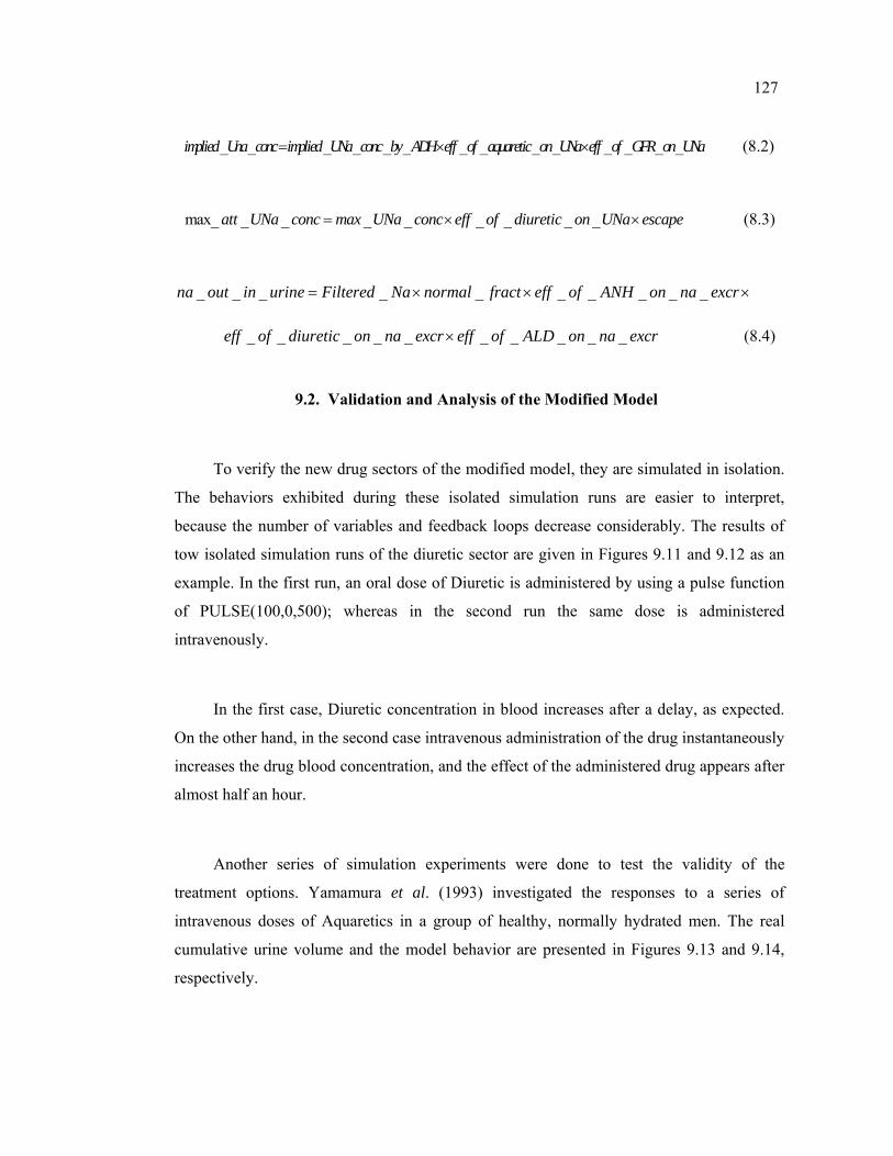
127
_ _ _ _ _ _ _ _ _ _ _ _ _ _implied Una conc implied UNa conc by ADH eff of aquaretic on UNa eff of GFR on UNa= × × (8.2)
max_ _ _ _ _ _ _ _ _att UNa conc max UNa conc eff of diuretic on UNa escape= × × (8.3)
_ _ _ _ _ _ _ _ _ _na out in urine Filtered Na normal fract eff of ANH on na excr= × × ×
_ _ _ _ _ _ _ _ _ _eff of diuretic on na excr eff of ALD on na excr× (8.4)
9.2. Validation and Analysis of the Modified Model
To verify the new drug sectors of the modified model, they are simulated in isolation.
The behaviors exhibited during these isolated simulation runs are easier to interpret,
because the number of variables and feedback loops decrease considerably. The results of
tow isolated simulation runs of the diuretic sector are given in Figures 9.11 and 9.12 as an
example. In the first run, an oral dose of Diuretic is administered by using a pulse function
of PULSE(100,0,500); whereas in the second run the same dose is administered
intravenously.
In the first case, Diuretic concentration in blood increases after a delay, as expected.
On the other hand, in the second case intravenous administration of the drug instantaneously
increases the drug blood concentration, and the effect of the administered drug appears after
almost half an hour.
Another series of simulation experiments were done to test the validity of the
treatment options. Yamamura et al. (1993) investigated the responses to a series of
intravenous doses of Aquaretics in a group of healthy, normally hydrated men. The real
cumulative urine volume and the model behavior are presented in Figures 9.13 and 9.14,
respectively.
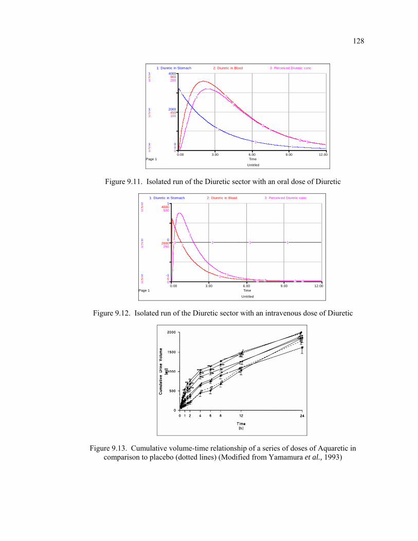
128
Untitled
Page 10.00 3.00 6.00 9.00 12.00
Time
1:
1:
1:
2:
2:
2:
3:
3:
3:
0
2000
4000
0
450
900
0
100
200
1: Diuretic in Stomach 2: Diuretic in Blood 3: Perceiv ed Diuretic conc
1
1
11
22
2
2
3
3
3
3
Figure 9.11. Isolated run of the Diuretic sector with an oral dose of Diuretic
Untitled
Page 10.00 3.00 6.00 9.00 12.00
Time
1:
1:
1:
2:
2:
2:
3:
3:
3:
-1
0
1
0
2000
4000
0
250
500
1: Diuretic in Stomach 2: Diuretic in Blood 3: Perceiv ed Diuretic conc
1 1 1 12
22 2
3
33 3
Figure 9.12. Isolated run of the Diuretic sector with an intravenous dose of Diuretic
Figure 9.13. Cumulative volume-time relationship of a series of doses of Aquaretic in comparison to placebo (dotted lines) (Modified from Yamamura et al., 1993)
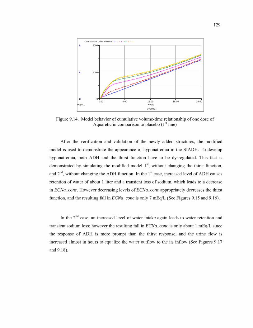
129
Untitled
Page 10.00 6.00 12.00 18.00 24.00
Hours
1:
1:
1:
0
1000
2000
Cumulativ e Urine Volume: 1 - 2 - 3 - 4 - 5 - 6 -
Figure 9.14. Model behavior of cumulative volume-time relationship of one dose of Aquaretic in comparison to placebo (1st line)
After the verification and validation of the newly added structures, the modified
model is used to demonstrate the appearance of hyponatremia in the SIADH. To develop
hyponatremia, both ADH and the thirst function have to be dysregulated. This fact is
demonstrated by simulating the modified model 1st, without changing the thirst function,
and 2nd, without changing the ADH function. In the 1st case, increased level of ADH causes
retention of water of about 1 liter and a transient loss of sodium, which leads to a decrease
in ECNa_conc. However decreasing levels of ECNa_conc appropriately decreases the thirst
function, and the resulting fall in ECNa_conc is only 7 mEq/L (See Figures 9.15 and 9.16).
In the 2nd case, an increased level of water intake again leads to water retention and
transient sodium loss; however the resulting fall in ECNa_conc is only about 1 mEq/L since
the response of ADH is more prompt than the thirst response, and the urine flow is
increased almost in hours to equalize the water outflow to the its inflow (See Figures 9.17
and 9.18).
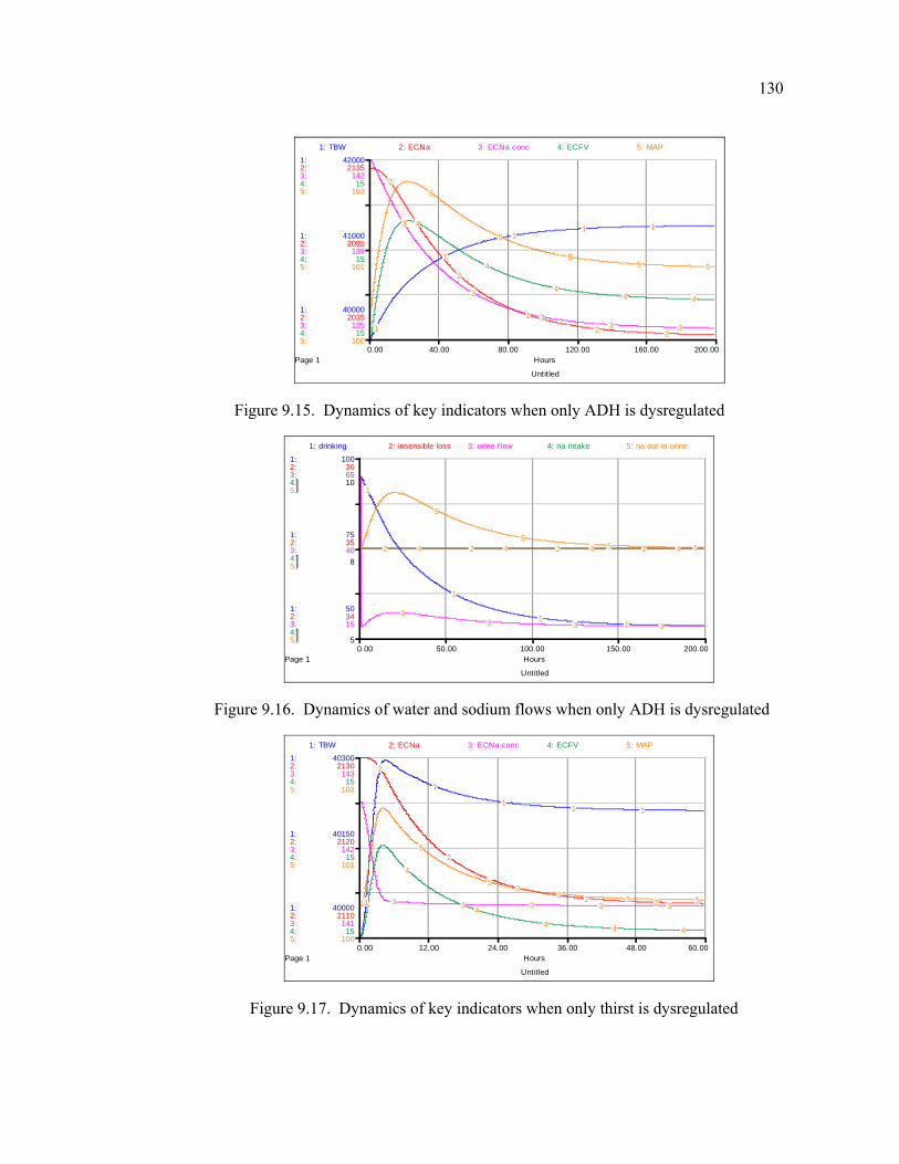
130
Untitled
Page 10.00 40.00 80.00 120.00 160.00 200.00
Hours
1:
1:
1:
2:
2:
2:
3:
3:
3:
4:
4:
4:
5:
5:
5:
40000
41000
42000
2035
2085
2135
135
139
142
15
15
15
100
101
103
1: TBW 2: ECNa 3: ECNa conc 4: ECFV 5: MAP
1
1
11 1
2
2
2
2 2
3
3
33 3
4
4
44 4
5
5
55 5
Figure 9.15. Dynamics of key indicators when only ADH is dysregulated
Untitled
Page 10.00 50.00 100.00 150.00 200.00
Hours
1:
1:
1:
2:
2:
2:
3:
3:
3:
4:
4:
4:
5:
5:
5:
50
75
100
34
35
36
15
40
65
5
8
10
1: drinking 2: insensible loss 3: urine f low 4: na intake 5: na out in urine
1
1
11
2 2 2 2
33 3 3
4 4 4 4
5
55 5
Figure 9.16. Dynamics of water and sodium flows when only ADH is dysregulated
Untitled
Page 10.00 12.00 24.00 36.00 48.00 60.00
Hours
1:
1:
1:
2:
2:
2:
3:
3:
3:
4:
4:
4:
5:
5:
5:
40000
40150
40300
2110
2120
2130
141
142
143
15
15
15
100
101
103
1: TBW 2: ECNa 3: ECNa conc 4: ECFV 5: MAP
1
1
11 1
2
2
22 23 3 3 3 3
4
4
4 4 4
5
55 5 5
Figure 9.17. Dynamics of key indicators when only thirst is dysregulated
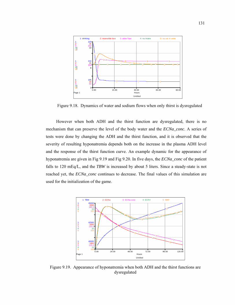
131
Untitled
Page 10.00 15.00 30.00 45.00 60.00
Hours
1:
1:
1:
2:
2:
2:
3:
3:
3:
4:
4:
4:
5:
5:
5:
195
210
225
34
35
36
50
150
250
5
8
10
1: drinking 2: insensible loss 3: urine f low 4: na intake 5: na out in urine
1
1 1 1
2 2 2 2
3 3 3 34 4 4 4
5
5 5 5
Figure 9.18. Dynamics of water and sodium flows when only thirst is dysregulated
However when both ADH and the thirst function are dysregulated, there is no
mechanism that can preserve the level of the body water and the ECNa_conc. A series of
tests were done by changing the ADH and the thirst function, and it is observed that the
severity of resulting hyponatremia depends both on the increase in the plasma ADH level
and the response of the thirst function curve. An example dynamic for the appearance of
hyponatremia are given in Fig 9.19 and Fig 9.20. In five days, the ECNa_conc of the patient
falls to 120 mEq/L, and the TBW is increased by about 5 liters. Since a steady-state is not
reached yet, the ECNa_conc continues to decrease. The final values of this simulation are
used for the initialization of the game.
Untitled
Page 10.00 24.00 48.00 72.00 96.00 120.00
Hours
1:
1:
1:
2:
2:
2:
3:
3:
3:
4:
4:
4:
5:
5:
5:
40000
42500
45000
1800
2000
2200
115.0
130.0
145.0
15
15
15
100
103
107
1: TBW 2: ECNa 3: ECNa conc 4: ECFV 5: MAP
1
1
1
1
1
2
2
2
2
2
3
3
3
3
3
4
4
44
4
5
55
5
5
Figure 9.19. Appearance of hyponatremia when both ADH and the thirst functions are dysregulated
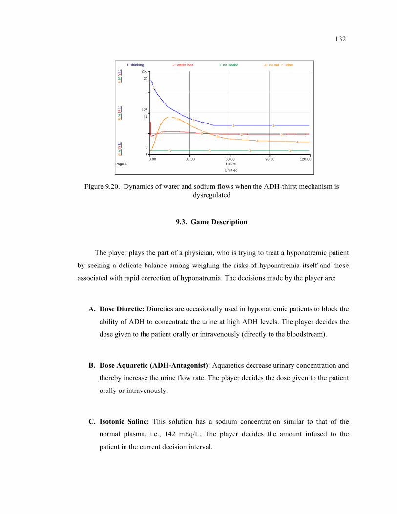
132
Untitled
Page 10.00 30.00 60.00 90.00 120.00
Hours
1:
1:
1:
2:
2:
2:
3:
3:
3:
4:
4:
4:
0
125
250
7
14
20
1: drinking 2: water lost 3: na intake 4: na out in urine
1
11 1
2 2 2 2
3 3 3 3
4
44 4
Figure 9.20. Dynamics of water and sodium flows when the ADH-thirst mechanism is dysregulated
9.3. Game Description
The player plays the part of a physician, who is trying to treat a hyponatremic patient
by seeking a delicate balance among weighing the risks of hyponatremia itself and those
associated with rapid correction of hyponatremia. The decisions made by the player are:
A. Dose Diuretic: Diuretics are occasionally used in hyponatremic patients to block the
ability of ADH to concentrate the urine at high ADH levels. The player decides the
dose given to the patient orally or intravenously (directly to the bloodstream).
B. Dose Aquaretic (ADH-Antagonist): Aquaretics decrease urinary concentration and
thereby increase the urine flow rate. The player decides the dose given to the patient
orally or intravenously.
C. Isotonic Saline: This solution has a sodium concentration similar to that of the
normal plasma, i.e., 142 mEq/L. The player decides the amount infused to the
patient in the current decision interval.
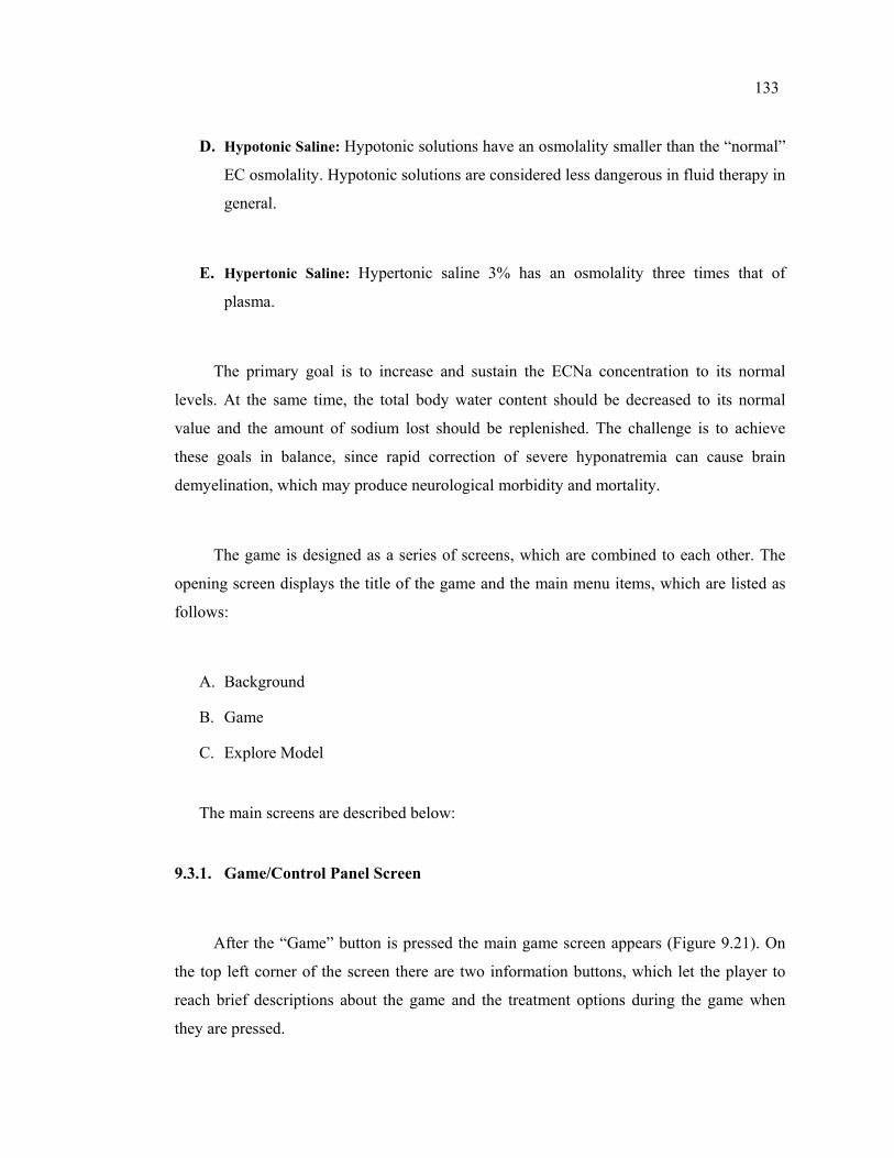
133
D. Hypotonic Saline: Hypotonic solutions have an osmolality smaller than the “normal”
EC osmolality. Hypotonic solutions are considered less dangerous in fluid therapy in
general.
E. Hypertonic Saline: Hypertonic saline 3% has an osmolality three times that of
plasma.
The primary goal is to increase and sustain the ECNa concentration to its normal
levels. At the same time, the total body water content should be decreased to its normal
value and the amount of sodium lost should be replenished. The challenge is to achieve
these goals in balance, since rapid correction of severe hyponatremia can cause brain
demyelination, which may produce neurological morbidity and mortality.
The game is designed as a series of screens, which are combined to each other. The
opening screen displays the title of the game and the main menu items, which are listed as
follows:
A. Background
B. Game
C. Explore Model
The main screens are described below:
9.3.1. Game/Control Panel Screen
After the “Game” button is pressed the main game screen appears (Figure 9.21). On
the top left corner of the screen there are two information buttons, which let the player to
reach brief descriptions about the game and the treatment options during the game when
they are pressed.
134
On the bottom right corner of the screen, the game controls are displayed. The game is
initiated by pressing the Start button in the New Game frame that is displayed at the bottom
right corner of the screen.
On the left side of the screen, the Decision Sliders are displayed. The player enters his
decisions by dragging the slider knob to the left or right using the cursor or by entering in
the small box below the slider knob. After the decisions are made, the Advance button
should be pressed. When this button is pressed the simulation advances 4 hours (which is
the default value and can be changed in the scenario settings) and the new values of the
variables are calculated. The simulation will pause automatically every 8 hour to let the
player change his decision settings and review data. Pressing the Record of Decisions
button on the top of the screen enables the player to examine the history of the decisions in
a graphical and tabular format.
Once a decision value is changed from its original value, a “U” appears at the bottom-
left corner of the slider. Clicking on it will reset the value to sliders’ original value. Clicking
on the “?” buttons on the sliders enables the player to reach more information about the
associated decision variable.
The total duration will be 120 hours, or 30 decision rounds. At the beginning of the
game, you can increase the decision period (or the pause interval) of the simulation from its
default value of 8 hours to 4 or 12 hours. The simulation time can be traced through the
displays that are located on the top right corner of the screen. At any time, the player can
quit the simulation by pressing the End Game button that is displayed at the bottom right
corner of the screen.
To start a new game the player should first terminate the current game pressing the
End Game button. Next, the model should be initialized to its original setting pressing the
Reset button in the New Game frame. Then a new game can be started pressing the Start
button in the same frame. Between two sequential games the model must be “Reset” first!
Otherwise the Start button would not work properly.
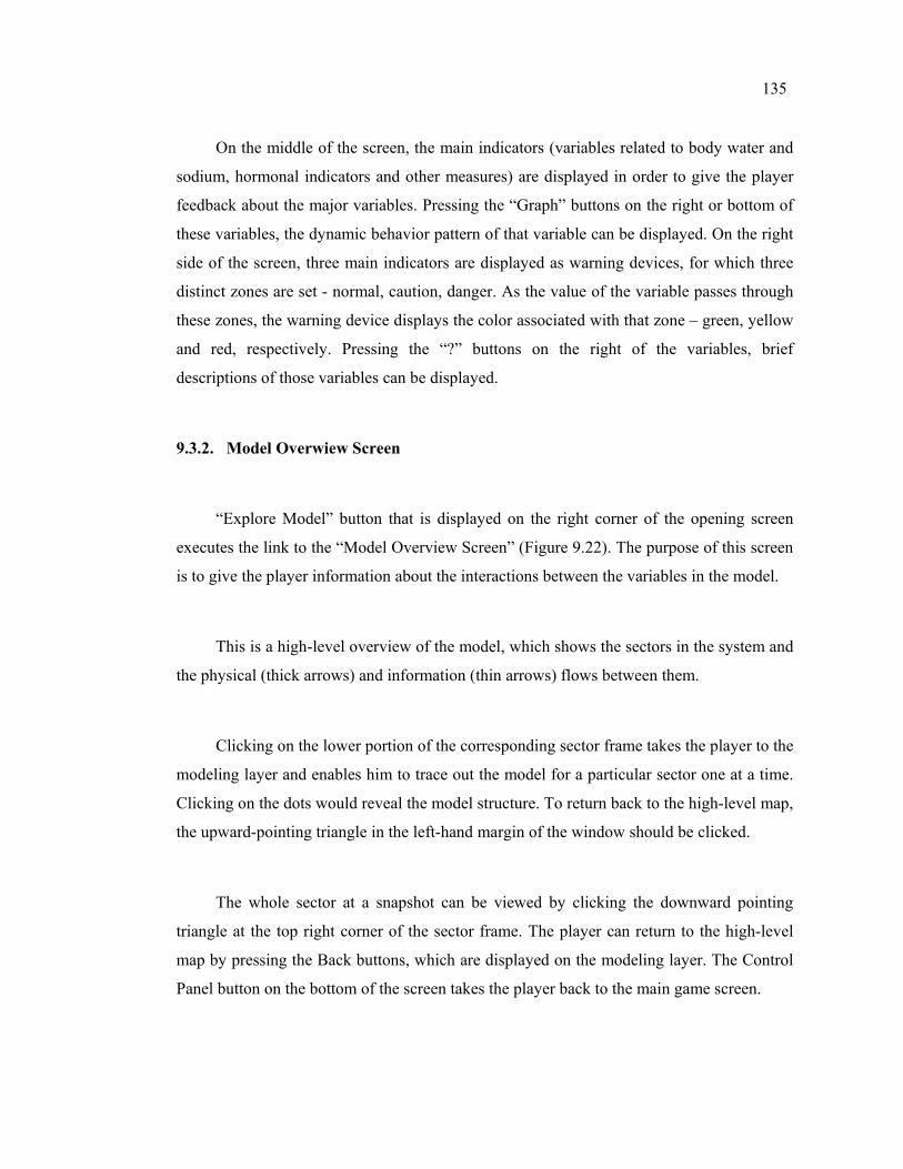
135
On the middle of the screen, the main indicators (variables related to body water and
sodium, hormonal indicators and other measures) are displayed in order to give the player
feedback about the major variables. Pressing the “Graph” buttons on the right or bottom of
these variables, the dynamic behavior pattern of that variable can be displayed. On the right
side of the screen, three main indicators are displayed as warning devices, for which three
distinct zones are set - normal, caution, danger. As the value of the variable passes through
these zones, the warning device displays the color associated with that zone – green, yellow
and red, respectively. Pressing the “?” buttons on the right of the variables, brief
descriptions of those variables can be displayed.
9.3.2. Model Overwiew Screen
“Explore Model” button that is displayed on the right corner of the opening screen
executes the link to the “Model Overview Screen” (Figure 9.22). The purpose of this screen
is to give the player information about the interactions between the variables in the model.
This is a high-level overview of the model, which shows the sectors in the system and
the physical (thick arrows) and information (thin arrows) flows between them.
Clicking on the lower portion of the corresponding sector frame takes the player to the
modeling layer and enables him to trace out the model for a particular sector one at a time.
Clicking on the dots would reveal the model structure. To return back to the high-level map,
the upward-pointing triangle in the left-hand margin of the window should be clicked.
The whole sector at a snapshot can be viewed by clicking the downward pointing
triangle at the top right corner of the sector frame. The player can return to the high-level
map by pressing the Back buttons, which are displayed on the modeling layer. The Control
Panel button on the bottom of the screen takes the player back to the main game screen.
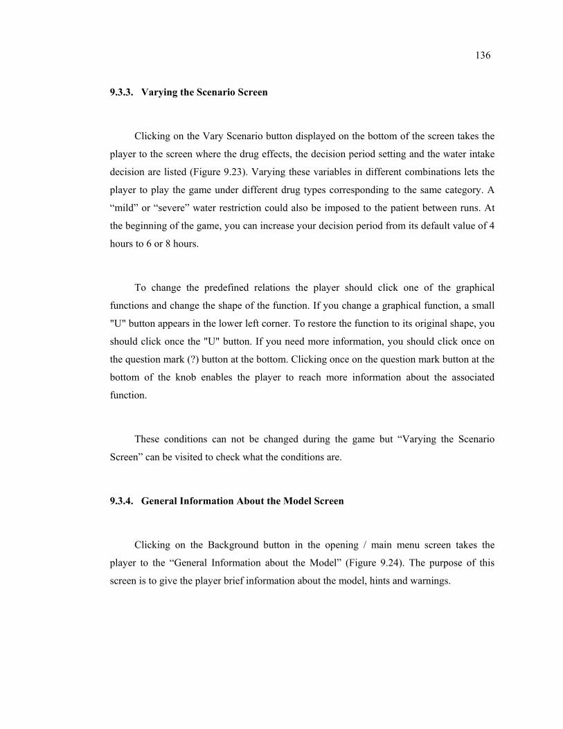
136
9.3.3. Varying the Scenario Screen
Clicking on the Vary Scenario button displayed on the bottom of the screen takes the
player to the screen where the drug effects, the decision period setting and the water intake
decision are listed (Figure 9.23). Varying these variables in different combinations lets the
player to play the game under different drug types corresponding to the same category. A
“mild” or “severe” water restriction could also be imposed to the patient between runs. At
the beginning of the game, you can increase your decision period from its default value of 4
hours to 6 or 8 hours.
To change the predefined relations the player should click one of the graphical
functions and change the shape of the function. If you change a graphical function, a small
"U" button appears in the lower left corner. To restore the function to its original shape, you
should click once the "U" button. If you need more information, you should click once on
the question mark (?) button at the bottom. Clicking once on the question mark button at the
bottom of the knob enables the player to reach more information about the associated
function.
These conditions can not be changed during the game but “Varying the Scenario
Screen” can be visited to check what the conditions are.
9.3.4. General Information About the Model Screen
Clicking on the Background button in the opening / main menu screen takes the
player to the “General Information about the Model” (Figure 9.24). The purpose of this
screen is to give the player brief information about the model, hints and warnings.
137
9.3.5. General Information About the Sliders Screen
Clicking on the About Controls button in the Control Panel takes the player to the
“General Information about Input Sliders” Screen (Figure 9.25). The purpose of this screen
is to give the player general information about the use of the sliders.
9.3.6. End Game Screens
Clicking on the End Game button initiates quitting process. Before exiting the game,
the player will be asked to save the game results in a file. If the player chooses to save the
game results, he will be asked to enter a name for the file, which will keep the data of the
current game results. It must have the extension “.stm” in Windows environment.
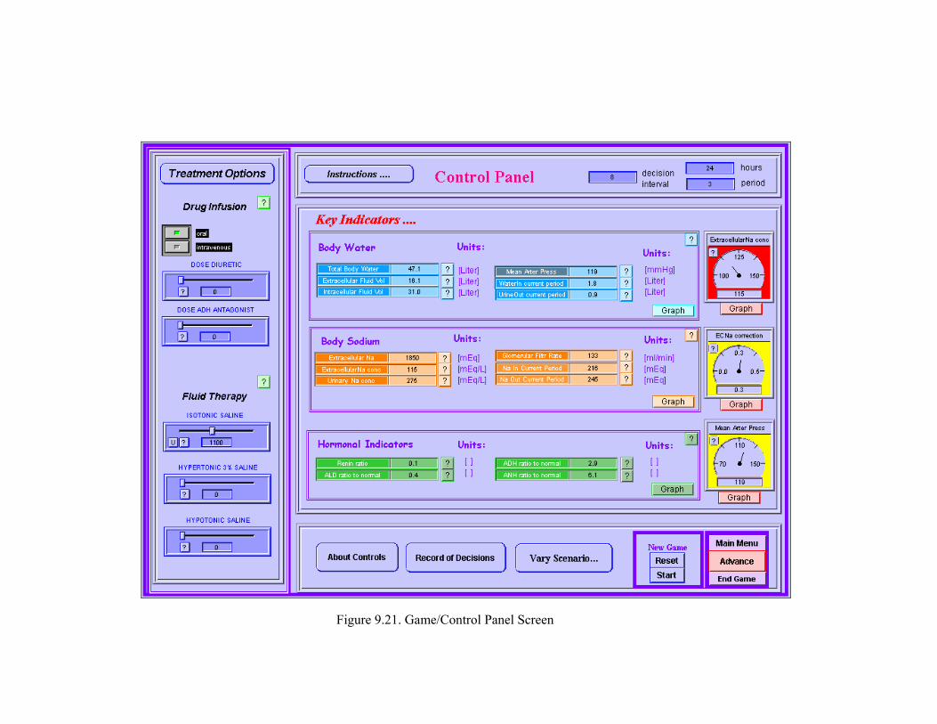
Figure 9.21. Game/Control Panel Screen
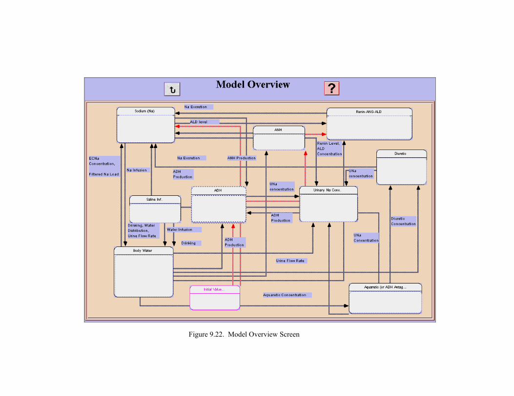
Figure 9.22. Model Overview Screen
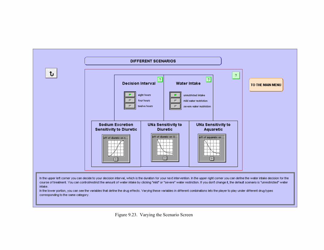
Figure 9.23. Varying the Scenario Screen
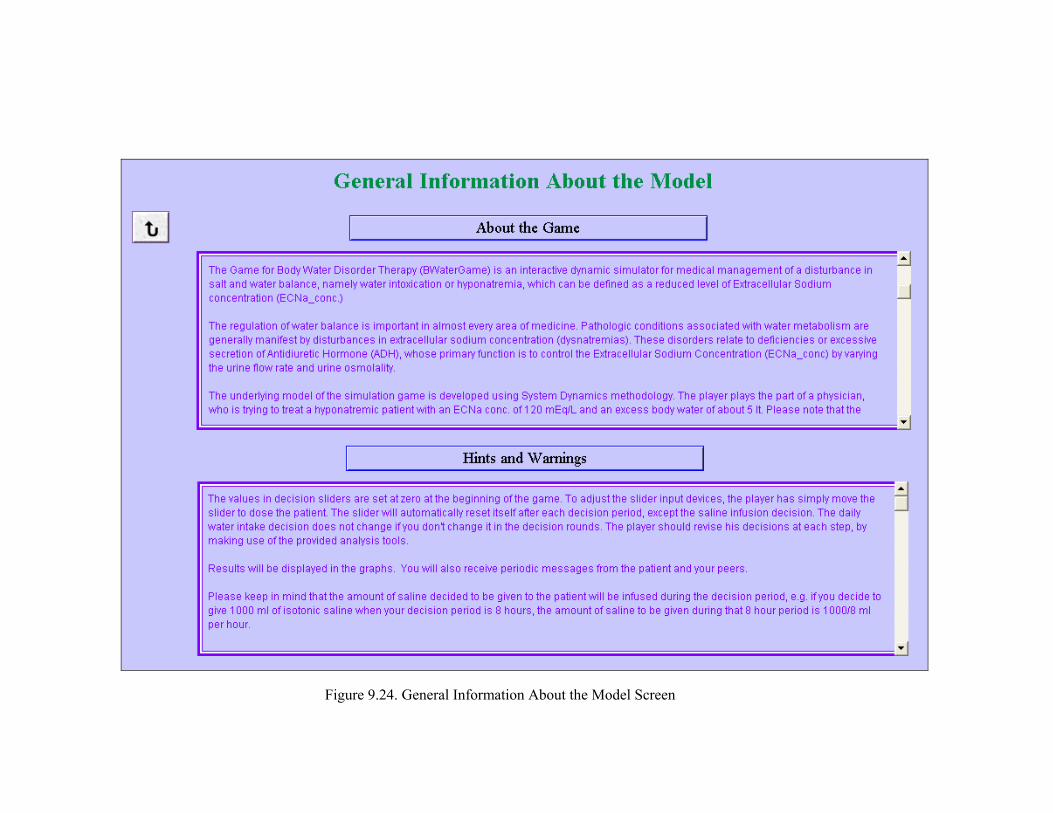
Figure 9.24. General Information About the Model Screen
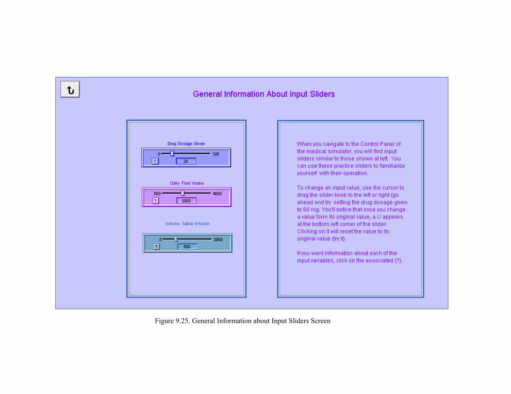
Figure 9.25. General Information about Input Sliders Screen
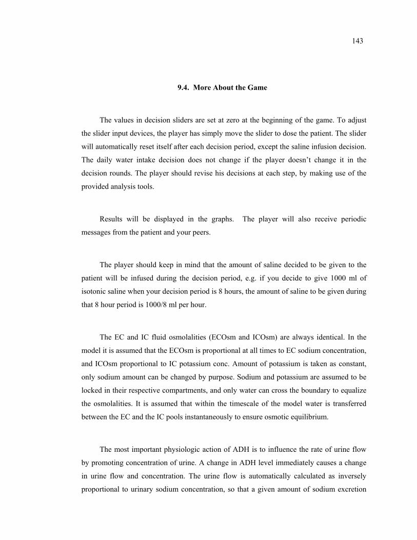
143
9.4. More About the Game
The values in decision sliders are set at zero at the beginning of the game. To adjust
the slider input devices, the player has simply move the slider to dose the patient. The slider
will automatically reset itself after each decision period, except the saline infusion decision.
The daily water intake decision does not change if the player doesn’t change it in the
decision rounds. The player should revise his decisions at each step, by making use of the
provided analysis tools.
Results will be displayed in the graphs. The player will also receive periodic
messages from the patient and your peers.
The player should keep in mind that the amount of saline decided to be given to the
patient will be infused during the decision period, e.g. if you decide to give 1000 ml of
isotonic saline when your decision period is 8 hours, the amount of saline to be given during
that 8 hour period is 1000/8 ml per hour.
The EC and IC fluid osmolalities (ECOsm and ICOsm) are always identical. In the
model it is assumed that the ECOsm is proportional at all times to EC sodium concentration,
and ICOsm proportional to IC potassium conc. Amount of potassium is taken as constant,
only sodium amount can be changed by purpose. Sodium and potassium are assumed to be
locked in their respective compartments, and only water can cross the boundary to equalize
the osmolalities. It is assumed that within the timescale of the model water is transferred
between the EC and the IC pools instantaneously to ensure osmotic equilibrium.
The most important physiologic action of ADH is to influence the rate of urine flow
by promoting concentration of urine. A change in ADH level immediately causes a change
in urine flow and concentration. The urine flow is automatically calculated as inversely
proportional to urinary sodium concentration, so that a given amount of sodium excretion
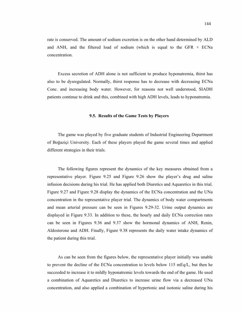
144
rate is conserved. The amount of sodium excretion is on the other hand determined by ALD
and ANH, and the filtered load of sodium (which is equal to the GFR × ECNa
concentration.
Excess secretion of ADH alone is not sufficient to produce hyponatremia, thirst has
also to be dysregulated. Normally, thirst response has to decrease with decreasing ECNa
Conc. and increasing body water. However, for reasons not well understood, SIADH
patients continue to drink and this, combined with high ADH levels, leads to hyponatremia.
9.5. Results of the Game Tests by Players
The game was played by five graduate students of Industrial Engineering Department
of Boğaziçi University. Each of these players played the game several times and applied
different strategies in their trials.
The following figures represent the dynamics of the key measures obtained from a
representative player. Figure 9.25 and Figure 9.26 show the player’s drug and saline
infusion decisions during his trial. He has applied both Diuretics and Aquaretics in this trial.
Figure 9.27 and Figure 9.28 display the dynamics of the ECNa concentration and the UNa
concentration in the representative player trial. The dynamics of body water compartments
and mean arterial pressure can be seen in Figures 9.29-32. Urine output dynamics are
displayed in Figure 9.33. In addition to these, the hourly and daily ECNa correction rates
can be seen in Figures 9.36 and 9.37 show the hormonal dynamics of ANH, Renin,
Aldosterone and ADH. Finally, Figure 9.38 represents the daily water intake dynamics of
the patient during this trial.
As can be seen from the figures below, the representative player initially was unable
to prevent the decline of the ECNa concentration to levels below 115 mEq/L, but then he
succeeded to increase it to mildly hyponatremic levels towards the end of the game. He used
a combination of Aquaretics and Diuretics to increase urine flow via a decreased UNa
concentration, and also applied a combination of hypertonic and isotonic saline during his
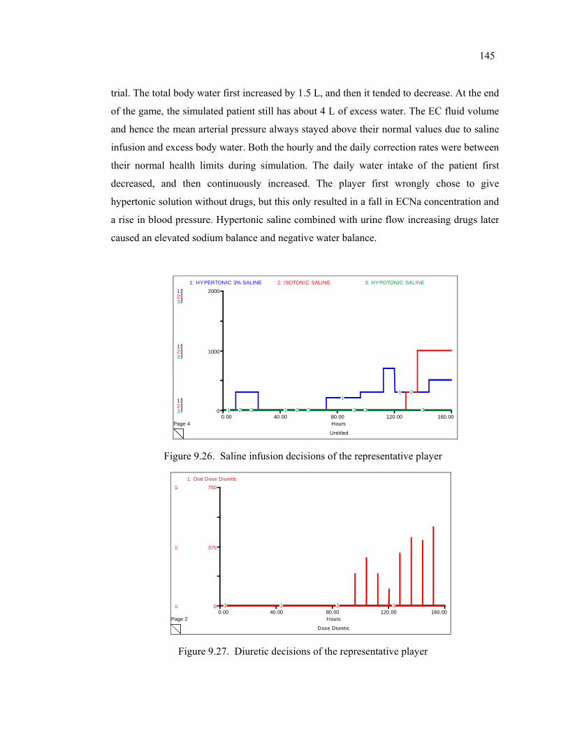
145
trial. The total body water first increased by 1.5 L, and then it tended to decrease. At the end
of the game, the simulated patient still has about 4 L of excess water. The EC fluid volume
and hence the mean arterial pressure always stayed above their normal values due to saline
infusion and excess body water. Both the hourly and the daily correction rates were between
their normal health limits during simulation. The daily water intake of the patient first
decreased, and then continuously increased. The player first wrongly chose to give
hypertonic solution without drugs, but this only resulted in a fall in ECNa concentration and
a rise in blood pressure. Hypertonic saline combined with urine flow increasing drugs later
caused an elevated sodium balance and negative water balance.
Untitled
Page 40.00 40.00 80.00 120.00 160.00
Hours
1:
1:
1:
2:
2:
2:
3:
3:
3:
0
1000
2000
1: HYPERTONIC 3% SALINE 2: ISOTONIC SALINE 3: HYPOTONIC SALINE
1 1
11
2 2 2
2
3 3 3 3
Figure 9.26. Saline infusion decisions of the representative player
Dose Diuretic
Page 20.00 40.00 80.00 120.00 160.00
Hours
1:
1:
1:
0
375
7501: Oral Dose Diuretic
1 1 1 1
Figure 9.27. Diuretic decisions of the representative player
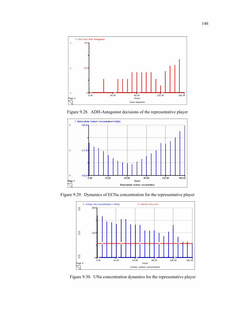
146
Dose Aquaretic
Page 30.00 40.00 80.00 120.00 160.00
Hours
1:
1:
1:
0
375
7501: Oral Dose ADH Antagonist
1 1 1 1
Figure 9.28. ADH-Antagonist decisions of the representative player
Figure 9.29. Dynamics of ECNa concentration for the representative player
Urinary sodium concentration
Page 40.00 32.00 64.00 96.00 128.00 160.00
Hours
1:
1:
1:
2:
2:
2:
0
225
450
1: Urinary Na Concentration \ mEq\L 2: Normal UNa conc
1 1 1 1 1
2 2 2 2 2
Figure 9.30. UNa concentration dynamics for the representative player
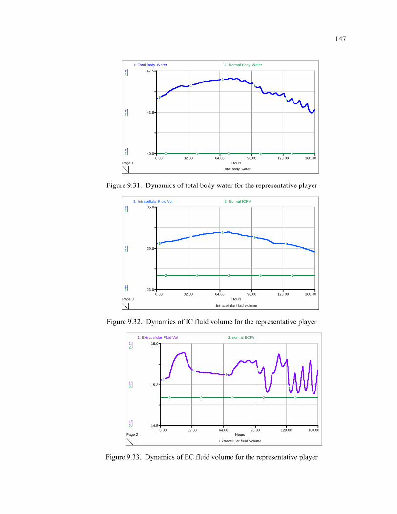
147
Total body water
Page 10.00 32.00 64.00 96.00 128.00 160.00
Hours
1:
1:
1:
2:
2:
2:
40.0
43.8
47.5
1: Total Body Water 2: Normal Body Water
1
11
1
1
2 2 2 2 2
Figure 9.31. Dynamics of total body water for the representative player
Intracellular f luid v olume
Page 30.00 32.00 64.00 96.00 128.00 160.00
Hours
1:
1:
1:
2:
2:
2:
23.0
29.0
35.0
1: Intracellular Fluid Vol 2: Normal ICFV
1
11
1
1
2 2 2 2 2
Figure 9.32. Dynamics of IC fluid volume for the representative player
Extracellular f luid v olume
Page 20.00 32.00 64.00 96.00 128.00 160.00
Hours
1:
1:
1:
2:
2:
2:
14.5
15.3
16.01: Extracellular Fluid Vol 2: normal ECFV
1
11
1
1
2 2 2 2 2
Figure 9.33. Dynamics of EC fluid volume for the representative player
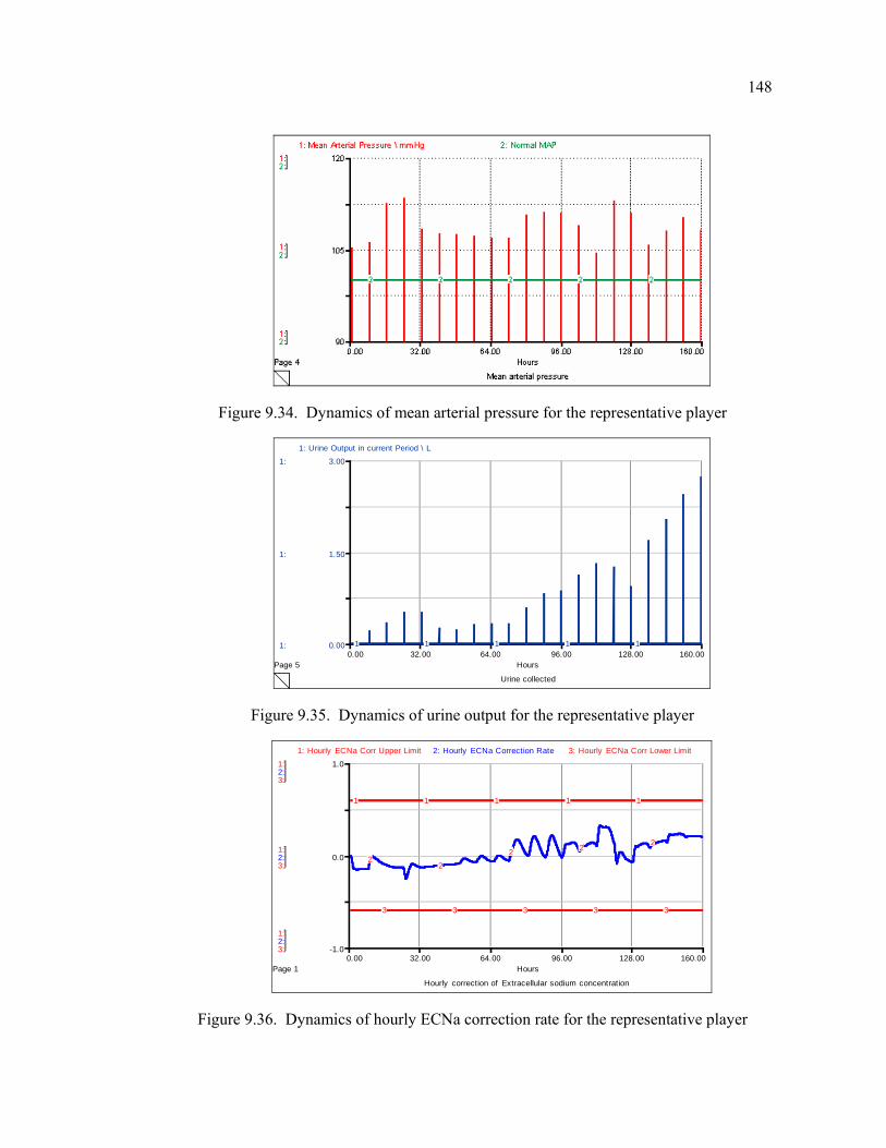
148
Figure 9.34. Dynamics of mean arterial pressure for the representative player
Urine collected
Page 50.00 32.00 64.00 96.00 128.00 160.00
Hours
1:
1:
1:
0.00
1.50
3.00
1: Urine Output in current Period \ L
1 1 1 1 1
Figure 9.35. Dynamics of urine output for the representative player
Hourly correction of Extracellular sodium concentration
Page 10.00 32.00 64.00 96.00 128.00 160.00
Hours
1:
1:
1:
2:
2:
2:
3:
3:
3:
-1.0
0.0
1.0
1: Hourly ECNa Corr Upper Limit 2: Hourly ECNa Correction Rate 3: Hourly ECNa Corr Lower Limit
1 1 1 1 1
22
2 2 2
3 3 3 3 3
Figure 9.36. Dynamics of hourly ECNa correction rate for the representative player
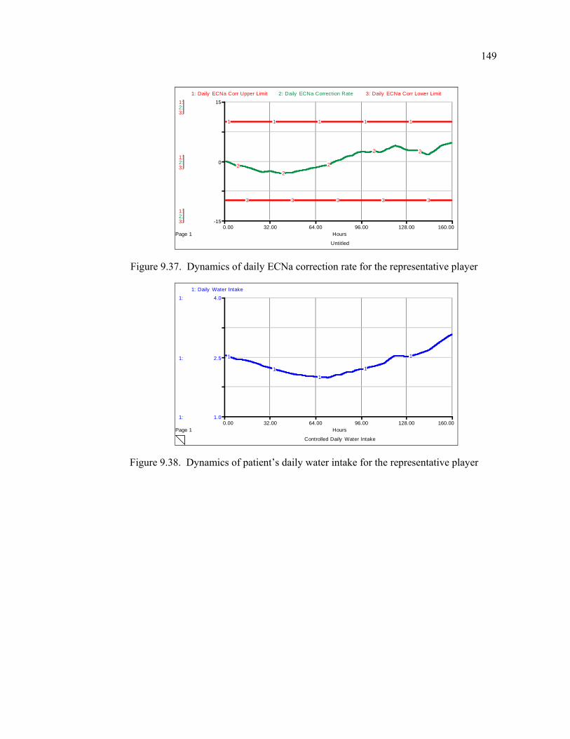
149
Untitled
Page 10.00 32.00 64.00 96.00 128.00 160.00
Hours
1:
1:
1:
2:
2:
2:
3:
3:
3:
-15
0
15
1: Daily ECNa Corr Upper Limit 2: Daily ECNa Correction Rate 3: Daily ECNa Corr Lower Limit
1 1 1 1 1
22
2
2 2
3 3 3 3 3
Figure 9.37. Dynamics of daily ECNa correction rate for the representative player
Controlled Daily Water Intake
Page 10.00 32.00 64.00 96.00 128.00 160.00
Hours
1:
1:
1:
1.0
2.5
4.0
1: Daily Water Intake
1
11
1
1
Figure 9.38. Dynamics of patient’s daily water intake for the representative player
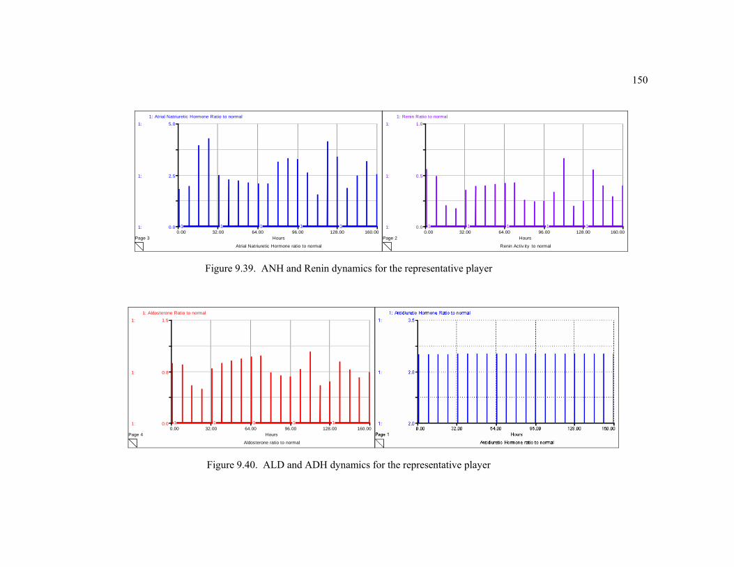
150
Atrial Natriuretic Hormone ratio to normal
Page 30.00 32.00 64.00 96.00 128.00 160.00
Hours
1:
1:
1:
0.0
2.5
5.01: Atrial Natriuretic Hormone Ratio to normal
1 1 1 1 1
Renin Activ ity to normal
Page 20.00 32.00 64.00 96.00 128.00 160.00
Hours
1:
1:
1:
0.0
0.5
1.01: Renin Ratio to normal
1 1 1 1 1
Figure 9.39. ANH and Renin dynamics for the representative player
Aldosterone ratio to normal
Page 40.00 32.00 64.00 96.00 128.00 160.00
Hours
1:
1:
1:
0.0
0.8
1.5
1: Aldosterone Ratio to normal
1 1 1 1 1
Figure 9.40. ALD and ADH dynamics for the representative player
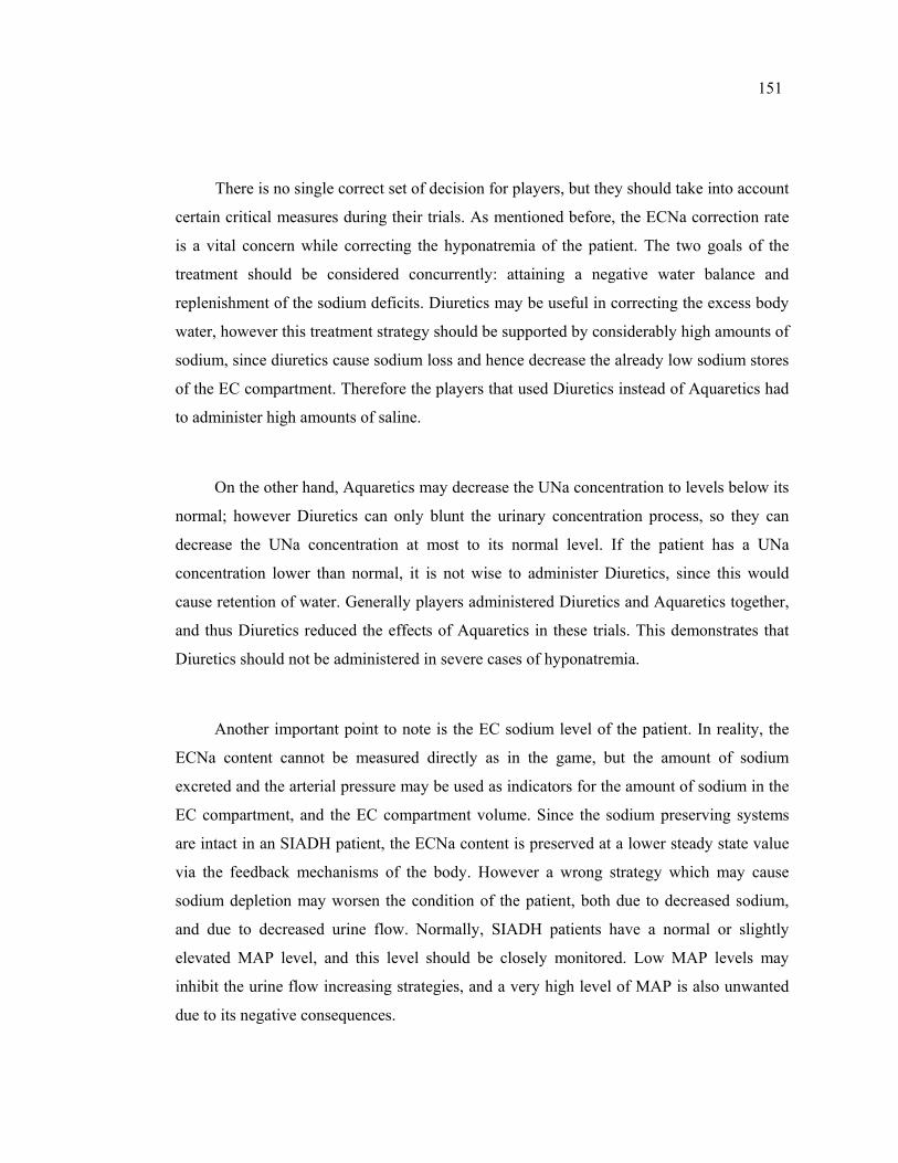
151
There is no single correct set of decision for players, but they should take into account
certain critical measures during their trials. As mentioned before, the ECNa correction rate
is a vital concern while correcting the hyponatremia of the patient. The two goals of the
treatment should be considered concurrently: attaining a negative water balance and
replenishment of the sodium deficits. Diuretics may be useful in correcting the excess body
water, however this treatment strategy should be supported by considerably high amounts of
sodium, since diuretics cause sodium loss and hence decrease the already low sodium stores
of the EC compartment. Therefore the players that used Diuretics instead of Aquaretics had
to administer high amounts of saline.
On the other hand, Aquaretics may decrease the UNa concentration to levels below its
normal; however Diuretics can only blunt the urinary concentration process, so they can
decrease the UNa concentration at most to its normal level. If the patient has a UNa
concentration lower than normal, it is not wise to administer Diuretics, since this would
cause retention of water. Generally players administered Diuretics and Aquaretics together,
and thus Diuretics reduced the effects of Aquaretics in these trials. This demonstrates that
Diuretics should not be administered in severe cases of hyponatremia.
Another important point to note is the EC sodium level of the patient. In reality, the
ECNa content cannot be measured directly as in the game, but the amount of sodium
excreted and the arterial pressure may be used as indicators for the amount of sodium in the
EC compartment, and the EC compartment volume. Since the sodium preserving systems
are intact in an SIADH patient, the ECNa content is preserved at a lower steady state value
via the feedback mechanisms of the body. However a wrong strategy which may cause
sodium depletion may worsen the condition of the patient, both due to decreased sodium,
and due to decreased urine flow. Normally, SIADH patients have a normal or slightly
elevated MAP level, and this level should be closely monitored. Low MAP levels may
inhibit the urine flow increasing strategies, and a very high level of MAP is also unwanted
due to its negative consequences.
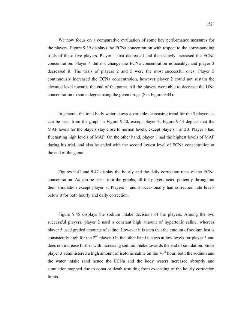
152
We now focus on a comparative evaluation of some key performance measures for
the players. Figure 9.39 displays the ECNa concentration with respect to the corresponding
trials of these five players. Player 1 first decreased and then slowly increased the ECNa
concentration. Player 4 did not change the ECNa concentration noticeably, and player 3
decreased it. The trials of players 2 and 5 were the most successful ones; Player 5
continuously increased the ECNa concentration, however player 2 could not sustain the
elevated level towards the end of the game. All the players were able to decrease the UNa
concentration to some degree using the given drugs (See Figure 9.44).
In general, the total body water shows a variable decreasing trend for the 5 players as
can be seen from the graph in Figure 9.40, except player 3. Figure 9.43 depicts that the
MAP levels for the players stay close to normal levels, except players 1 and 3. Player 3 had
fluctuating high levels of MAP. On the other hand, player 1 had the highest levels of MAP
during his trial, and also he ended with the second lowest level of ECNa concentration at
the end of the game.
Figures 9.41 and 9.42 display the hourly and the daily correction rates of the ECNa
concentration. As can be seen from the graphs, all the players acted patiently throughout
their simulation except player 3. Players 1 and 3 occasionally had correction rate levels
below 0 for both hourly and daily correction.
Figure 9.45 displays the sodium intake decisions of the players. Among the two
successful players, player 2 used a constant high amount of hypertonic saline, whereas
player 5 used graded amounts of saline. However it is seen that the amount of sodium lost is
consistently high for the 2nd player. On the other hand it stays at low levels for player 5 and
does not increase further with increasing sodium intake towards the end of simulation. Since
player 3 administered a high amount of isotonic saline on the 76th hour, both the sodium and
the water intake (and hence the ECNa and the body water) increased abruptly and
simulation stopped due to coma or death resulting from exceeding of the hourly correction
limits.
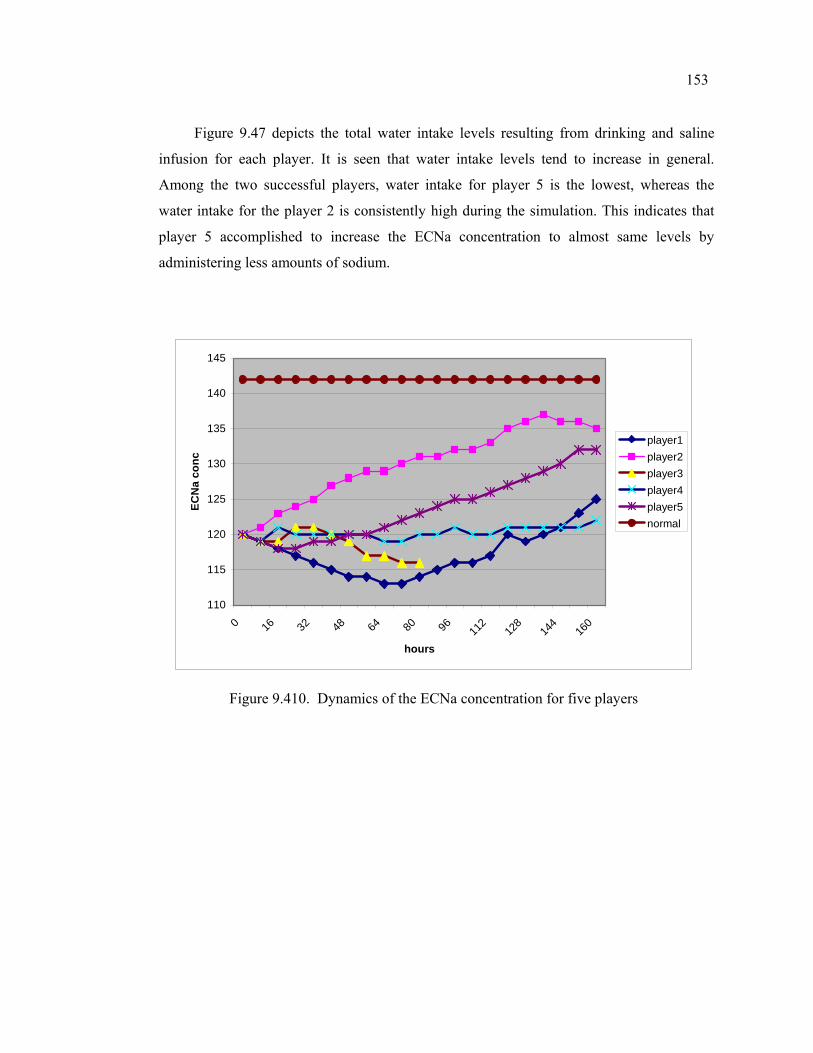
153
Figure 9.47 depicts the total water intake levels resulting from drinking and saline
infusion for each player. It is seen that water intake levels tend to increase in general.
Among the two successful players, water intake for player 5 is the lowest, whereas the
water intake for the player 2 is consistently high during the simulation. This indicates that
player 5 accomplished to increase the ECNa concentration to almost same levels by
administering less amounts of sodium.
110
115
120
125
130
135
140
145
0 16 32 48 64 80 96 112
128
144
160
hours
ECN
a co
nc
player1player2player3player4player5normal
Figure 9.410. Dynamics of the ECNa concentration for five players
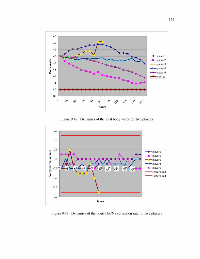
154
39
40
41
42
43
44
45
46
47
48
0 16 32 48 64 80 96 112
128
144
160
hours
Bod
y W
ater
player1player2player3player4player5normal
Figure 9.42. Dynamics of the total body water for five players
-0.7
-0.5
-0.3
-0.1
0.1
0.3
0.5
0.7
hours
hour
ly c
orre
ctio
n ra
te player1player2player3player4player5Lower LimitUpper Limit
Figure 9.43. Dynamics of the hourly ECNa correction rate for five players
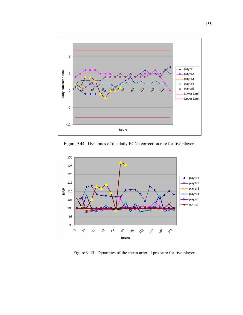
155
-12
-7
-2
3
8
8 24 40 56 72 88 104
120
136
152
hours
daily
cor
rect
on ra
te
player1player2player3player4player5Lower LimitUpper Limit
Figure 9.44. Dynamics of the daily ECNa correction rate for five players
90
95
100
105
110
115
120
125
130
0 16 32 48 64 80 96 112
128
144
160
hours
MA
P
player1
player2
player3
player4
player5
normal
Figure 9.45. Dynamics of the mean arterial pressure for five players
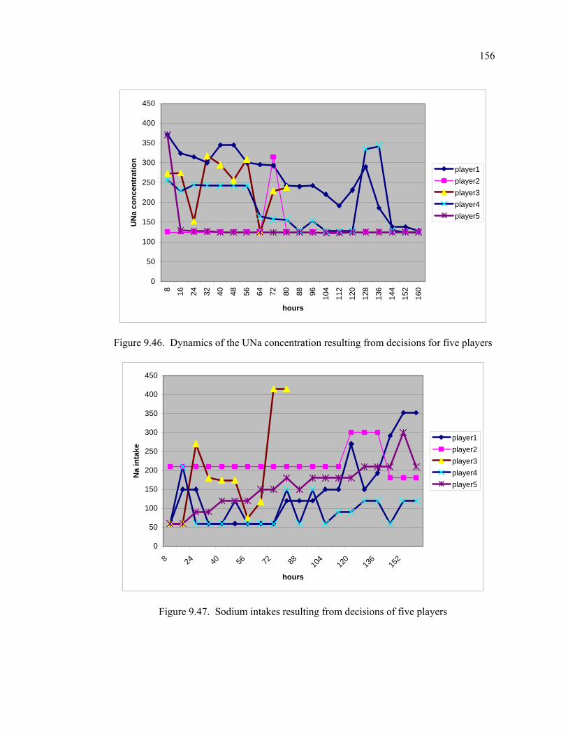
156
0
50
100
150
200
250
300
350
400
450
8 16 24 32 40 48 56 64 72 80 88 96 104
112
120
128
136
144
152
160
hours
UN
a co
ncen
trat
ion
player1player2player3player4player5
Figure 9.46. Dynamics of the UNa concentration resulting from decisions for five players
0
50
100
150
200
250
300
350
400
450
8 24 40 56 72 88 104
120
136
152
hours
Na
inta
ke
player1player2player3player4player5
Figure 9.47. Sodium intakes resulting from decisions of five players
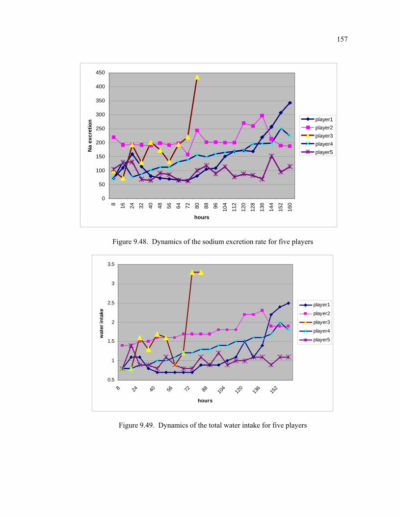
157
0
50
100
150
200
250
300
350
400
450
8 16 24 32 40 48 56 64 72 80 88 96 104
112
120
128
136
144
152
160
hours
Na
excr
etio
n player1player2player3player4player5
Figure 9.48. Dynamics of the sodium excretion rate for five players
0.5
1
1.5
2
2.5
3
3.5
8 24 40 56 72 88 104
120
136
152
hours
wat
er in
take
player1
player2
player3
player4
player5
Figure 9.49. Dynamics of the total water intake for five players
158
10. CONCLUSIONS AND FURTHER RESEARCH
The purpose of this research is to study the normal and disease physiology of the body
water metabolism, and to develop an interactive simulation model for a particular body fluid
disorder, namely water intoxication/hyponatremia. For this purpose, a system dynamics
model is built representing the structure of the body water and sodium balance for a normal
individual. Then, this model is modified to include the effects of disease processes, and
example dynamics are reproduced for the development of ADH-induced hyponatremia.
Finally, a game version of the modified model is constructed by including the most relevant
treatment options, and possible necessary measurements for diagnosis. The game is then
used as an experiment platform to test and compare the possible effects of a given set of
treatment options on a simulated patient. This interactive simulation game attempts to be a
step towards a closed-loop therapy for the hyponatremia patients. It can also be used as a
learning and teaching environment for the renal physiology, and especially for the
differentiation between the concepts of “sodium content” and “sodium concentration”, and
related disorders.
The normal physiology of the body water metabolism entails an understanding of two
distinct but interactive homeostatic systems: the systems that regulate the extracellular
sodium concentration/body water content and the systems that regulate the blood
volume/sodium content. The mechanism for the regulation of water balance is often referred
to as the ‘thirst-ADH mechanism’. This system regulates water intake by controlling the
perception of thirst, and water output by ADH, which is responsible for the urinary
concentration and dilution. On the other hand, the main feedback mechanisms for sodium
balance include the ALD, the ANH, and the renal mechanisms.
As a result of extensive validity testing, the model is found to be a robust
representation of the water-electrolyte balance in normal and various test conditions. The
model demonstrates that ADH is extremely important for the control of sodium
concentration, yet it has a relatively mild effect on the control of blood volume/pressure. On
the other hand, arterial pressure is mainly determined by “sodium intake”, rather than water
159
intake, which at first seems paradoxical, since arterial pressure is in fact determined by the
“water volume” of the extracellular compartment. The study also depicts that excessive
secretion of either ADH or ALD does not increase body fluid volumes infinitely, since the
effects known as ‘ADH escape’ and ‘ALD escape’ protect the body from retention of high
levels of water. The compensating mechanisms for escape mainly change the sodium
excretion rate or the urinary concentration in the absence/excess of these hormones, so as to
return the body fluid balance to its normal. Therefore it can be concluded that conserving
the body fluid balance is a preliminary to conserve a constant blood pressure or a constant
blood sodium concentration.
The modified model for the development of hyponatremia reproduces all the cardinal
features of the SIADH. As in the reality, dysregulated ADH-thirst system first causes an
increase in the body fluids, but when the part retained in the extracellular fluid is sufficient
to activate volume receptors, transient sodium loss is promoted, and the extracellular
volume is only slightly elevated, despite the apparent expansion of the total body water.
Hence, it is the intracellular compartment which is mostly expanded in SIADH. As a result
of dilution, extracellular sodium concentration falls drastically. The arterial pressure is also
slightly elevated, and this causes an increase in the glomerular filtration rate. Moreover,
urine is still highly concentrated due to the absent negative feedback between the
extracellular sodium concentration and the ADH.
The interactive simulation game version yields meaningful results for various
treatment options. Game results reveal that the effective correction of the SIADH can only
be attained if a negative water balance can be maintained. Replacing the sodium deficits
alone is worthless since blood volume/pressure conserving mechanisms cause an increased
sodium excretion rate following the intake. Moreover, it is demonstrated that graded doses
of hypertonic saline infusion is the most useful solution for the treatment. However it
should be administered carefully to prevent an overcorrection, and concurrently with drugs
that increase the urine flow. It is also depicted that ADH-Antagonists are superior over
diuretics in SIADH in preventing intracellular edema. However diuretics could be used as
an adjunct to Aquaretics in certain edema forming conditions, since a sodium diuresis is
160
desirable in these conditions. In conclusion, the model and the game version constitute an
experimental laboratory for a closed-loop therapy approach to hyponatremia.
There are several avenues in which this research can be expanded. One first step is
converting the current game model for the treatment of severe hyponatremia in an intensive
care unit setting, by changing the initial conditions of the modified model and the treatment
options. Moreover, more realistic initial conditions could be selected to represent a person
who is inclined to become hyponatremic. Drinking structure of the model could also be
modified to be more realistic about the normal physiology. As mentioned before, short term
drinking feedbacks exist, e.g. the gastric feedback which prevents an overly high water
intake in a short time period.
Since the focus of the modified model is the development and therapy of
hyponatremia, other electrolytes have not been analyzed. The model can be extended to
incorporate potassium dynamics, since sodium and potassium regulatory systems are
coupled with the levels of aldosterone. In fact, hyponatremia occurs with many other
electrolyte imbalances, and hypokalemia (low levels of extracellular potassium
concentration) is the most common electrolyte disorder. Under normal conditions the
extracellular potassium dynamics is tightly controlled, since changes in the potassium
concentration have an important influence on cellular hydration, and most significantly in
the heart as a cause of cardiac arrest (Northrop, 2000). Moreover, pharmacological means
to correct hyponatremia often have a reverse effect on the potassium metabolism. For
instance, diuretics are known also to increase the potassium excretion, along with many
other electrolytes. An analysis of impacts of the treatment options of hyponatremia on
potassium dynamics may reveal a broader range of possible physiological phenomena.
Another important electrolyte excluded from this study is the urea. We have assumed
that urine osmolality is only determined by the sodium chloride; however in reality urea
also contributes to 40 percent of the urine osmolality when the kidney is forming a
maximally concentrated urine (Guyton, 2000). In SIADH, plasma urea concentration is
unusually low due to the excess body water and the rise in the glomerular filtration.
161
Moreover, urea is also used for the therapy of SIADH, and it is demonstrated that oral urea
is efficient in producing a high osmotic diuresis in patients with the SIADH (Decaux, 1981).
The rate of solute excretion is another determinant of the final urine osmolality. The
kidney can play with the concentration of urine at relatively low rates of solute excretion,
i.e. it can concentrate or dilute urine maximally. However at greater rates of solute
excretion, the ability of the kidney to modify the final osmolality of urine becomes
progressively blunted. Stated in another way, as solute excretion rate increases, the
osmolality of either a hypotonic or a hypertonic urine approaches that of plasma, regardless
of the circulating ADH level. This property allows for instance urea to be a safe and
effective treatment of the SIADH.
162
APPENDIX A: USER GUIDE OF BWATERGAME
The Game for Body Water Disorder Therapy (BWaterGame) is an interactive
dynamic simulator for medical management of a disturbance in salt and water balance,
namely water intoxication or hyponatremia, which can be defined as a reduced level of
Extracellular Sodium concentration (ECNa_conc.)
The regulation of water balance is important in almost every area of medicine.
Pathologic conditions associated with water metabolism are generally manifest by
disturbances in extracellular sodium concentration (dysnatremias). These disorders relate to
deficiencies or excessive secretion of Antidiuretic Hormone (ADH), whose primary
function is to control the Extracellular Sodium Concentration (ECNa_conc) by varying the
urine flow rate and urine osmolality.
The underlying model of the simulation game is developed using System Dynamics
methodology. The player plays the part of a physician, who is trying to treat a hyponatremic
patient with an ECNa conc. of 120 mEq/L and an excess body water of about 5 lt. Please
note that the “normal” level of plasma sodium is 142 mEq/L. While hyponatremia is
defined as an ECNa conc less than 135 mmol/l, clinical symptoms are seldom seen when
the serum sodium is greater than 125 mmol/l and are generally seen with a sodium less than
120 mmol/l. At values below 110 mmol/l, patients frequently die sudden deaths because of
coma and convulsions.
The primary goal is to increase and sustain the Extracellular Sodium
Concentration (ECNa_conc.) to its normal levels, which is about 140 mEq/L. At the
same time, the total body water content should be decreased to its normal value of 40
liters as well as the extracellular & the intracellular water volumes. The challenge is to
achieve these goals in balance, since rapid correction of severe hyponatremia can cause
brain demyelination (brain edema and subsequent neurologic consequences), which may
produce neurological morbidity and mortality.
163
The player should seek a delicate balance among weighing the risks of hyponatremia
itself and those associated with rapid correction of hyponatremia. A low ECNa_conc. is
associated with an increasing rate of mortality. Depending on the degree of water retention,
weakness and muscle cramps may develop, followed by confusion (“water intoxication”),
convulsions, coma and death. On the other hand, irreversible neurological damage and
death may also occur when the ECNa conc. is rapidly corrected.
Excessive or inappropriate production of ADH- Syndrome of Inappropriate ADH
secretion (SIADH), predisposes to hyponatremia, reflecting water retention. SIADH is the
prototypical disorder for hyponatremia. The patient in the game has water retention and
consequently severe hyponatremia due to SIADH of unknown reason. Cardinal features of
the SIADH are: Hyponatremia, urine osmolality greater than plasma osmolality, excessive
renal sodium excretion, absence of hypotension, hypovolemia, and edema-forming states.
The diagnosis and treatment of hyponatremia is also often challenging and can add to
the problem if inappropriately managed, since many and sometimes complex factors
influence the ECNa conc. One should always keep in mind that the system that regulates
total body water and ECNa conc. is a multiple input/multiple output system and is cross-
coupled with systems that regulate the mean arterial pressure (MAP).
Player Decisions
To date physicians have two main options in treating hyponatremia: a) They can try to
limit fluid intake, and b) they can reduce ADH or its effect in the kidney. When the primary
cause of the disorder cannot be treated, water restriction is the present mainstay of
treatment. Compliance with water restriction is poor, however; because it is impractical,
inefficient and difficult for the physician and the patient alike. Therefore water restriction is
presented only as an option in the scenario settings of the game.
The decisions made by the player can be of two types: The player may choose to give
the patient a drug, namely a “diuretic” and/or an “ADH Antagonist” (also known as
164
Aquaretics) to the patient. The main effect of these drugs is to change the urinary
concentration; however they may have side effects which will be explained below.
Fluid therapy (or saline infusion) constitutes another important part of the current
standard therapy for treating hyponatremia. It simply means to give water to the patient with
different concentrations of sodium. Since various types of intravenous fluids exist; the three
most commonly used categories are presented in the model, namely hypertonic, isotonic,
and hypotonic fluids, which are classified according to their sodium content. Though fluid
therapy is an important and quite ordinary therapeutic means, many problems are still
associated with it.
(A) Dose Diuretic: Diuretics are occasionally used in hyponatremic patients to block
the ability of ADH to concentrate the urine at high ADH levels. You should note that this
drug prevents formation of a concentrated urine and “lowers” the urine osmolality only
when the urine is more concentrated than normal. Moreover, diuretics have well known
side-effects: They cause significant urinary losses of sodium, potassium, and magnesium. In
this model, only sodium and potassium ions are presented and the level of potassium ions is
taken as constant. The player decides the dose given to the patient orally or intravenously
(directly to the bloodstream). The effect of diuretics occurs in a dose-dependent manner.
(B) Dose ADH Antagonist: Antidiuretic Hormone Antagonists (also known as
Aquaretics) are another category of drugs which can be used in the management of patients
with water excess and consequent dilutional hyponatremia, as in patients with congestive
heart failure and cirrhosis, or in patients with euvolemic hyponatremia, as in patients with
Syndrome of Inappropriate Antidiuretic Hormone (SIADH). These agents have been termed
“aquaretics” because of their ability to increase urine flow rate without affecting sodium
excretion. However it is seen that at higher doses they increase the current plasma ADH
levels also, which is a complication related to their usage. The player decides the dose given
to the patient orally or intravenously. Since their effect occurs in a dose-dependent manner
like diuretics, one should pay attention not to cause dehydration while trying to increase the
urine flow.
165
(C) Isotonic (or Normal) Saline: This solution has an [Na+] conc. similar to that of
the normal plasma.
(D) Hypotonic Saline: Hypotonic solutions vary between 0.45% and 0,18 % saline
(77 and 30 mEq/L Na). They have an osmolality smaller than the “normal” plasma
osmolality. Hypotonic solutions are considered less dangerous in fluid therapy in general.
(E) Hypertonic Saline: Hypertonic saline 3% has an osmolality three times that of
plasma. You should note that the percentage of sodium included in hypertonic saline is
biggest, but if given, one should consider that it also carries the biggest risk of causing an
overcorrection rate if used in inappropriately high amounts.
Starting the Game
The user must have Stella® Research Version 5.1 or later installed in his computer in
order to play the game. The game can be started by double clicking the “BWaterGame” icon
Logical Flow of the Game
The game is designed as a series of screens, which are connected to each other. The
opening screen displays the title of the game and the main menu items, which are listed as
follows:
(A) Background
(B) Game
(C) Explore Model
(D) Quit Game
Running a New Game
166
After the “Experiment” button is pressed the main game screen appears. In the top left
corner of the screen are two information buttons, which let the player to reach brief
instructions about the game and the decisions during the game when they are pressed.
On the bottom right corner of the screen, the game controls are displayed. The game is
initiated by pressing the Reset and Start buttons in the New Game that is displayed at the
bottom right corner of the screen.
On the left side of the screen, the Decision Sliders are displayed. After the decisions
are made, the Advance button should be pressed. When this button is pressed the simulation
advances 8 hours (which is the default value and can be changed in the scenario settings)
and the new values of the variables are calculated. The simulation will pause automatically
every 8 hour to let the player change his decision settings and review data. Pressing the
Record of Decisions button on the top of the screen enables the player to examine the
history of the decisions in a graphical and tabular format and pressing the Graph buttons in
the Body Water and Body Sodium frames enables the player to review the related body
water and sodium indicators measured between the periods.
Once a decision value is changed from its original value, a “U” appears at the bottom-
left corner of the slider. Clicking on it will reset the value to sliders’ original value. Clicking
on the “?” buttons on the sliders enables the player to reach more information about the
associated decision variable.
The total duration will be 160 hours, or 20 decision rounds. At the beginning of the
game, you can increase the decision period (or the pause interval) of the simulation from its
default value of 8 hours to 4 or 12 hours. The simulation time can be traced through the
displays that are located on the top right corner of the screen. At any time, the player can
quit the simulation by pressing the End Game button that is displayed at the bottom right
corner of the screen.
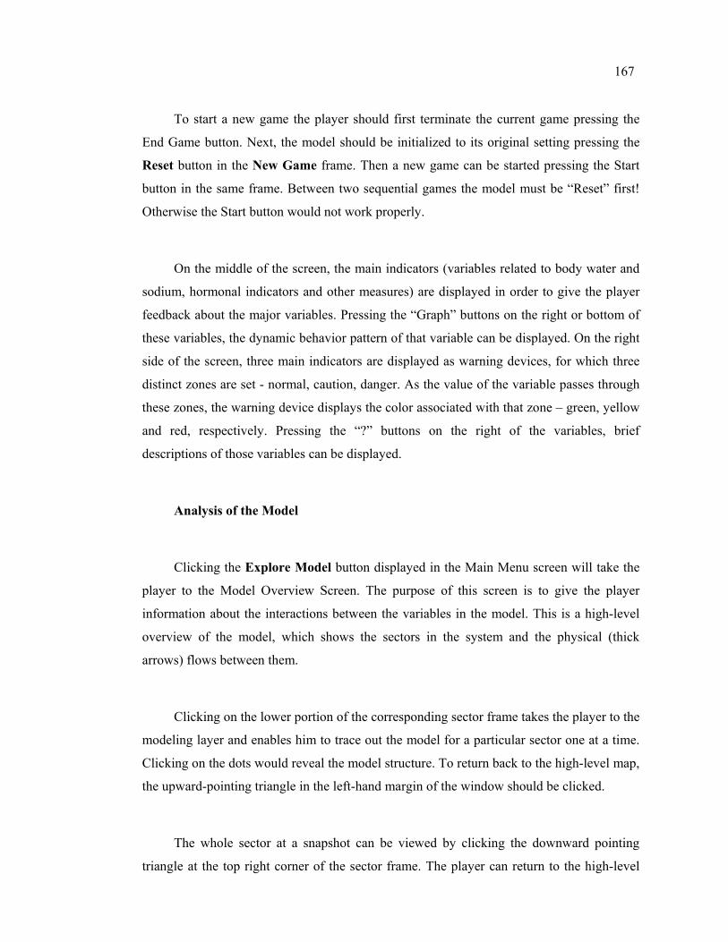
167
To start a new game the player should first terminate the current game pressing the
End Game button. Next, the model should be initialized to its original setting pressing the
Reset button in the New Game frame. Then a new game can be started pressing the Start
button in the same frame. Between two sequential games the model must be “Reset” first!
Otherwise the Start button would not work properly.
On the middle of the screen, the main indicators (variables related to body water and
sodium, hormonal indicators and other measures) are displayed in order to give the player
feedback about the major variables. Pressing the “Graph” buttons on the right or bottom of
these variables, the dynamic behavior pattern of that variable can be displayed. On the right
side of the screen, three main indicators are displayed as warning devices, for which three
distinct zones are set - normal, caution, danger. As the value of the variable passes through
these zones, the warning device displays the color associated with that zone – green, yellow
and red, respectively. Pressing the “?” buttons on the right of the variables, brief
descriptions of those variables can be displayed.
Analysis of the Model
Clicking the Explore Model button displayed in the Main Menu screen will take the
player to the Model Overview Screen. The purpose of this screen is to give the player
information about the interactions between the variables in the model. This is a high-level
overview of the model, which shows the sectors in the system and the physical (thick
arrows) flows between them.
Clicking on the lower portion of the corresponding sector frame takes the player to the
modeling layer and enables him to trace out the model for a particular sector one at a time.
Clicking on the dots would reveal the model structure. To return back to the high-level map,
the upward-pointing triangle in the left-hand margin of the window should be clicked.
The whole sector at a snapshot can be viewed by clicking the downward pointing
triangle at the top right corner of the sector frame. The player can return to the high-level
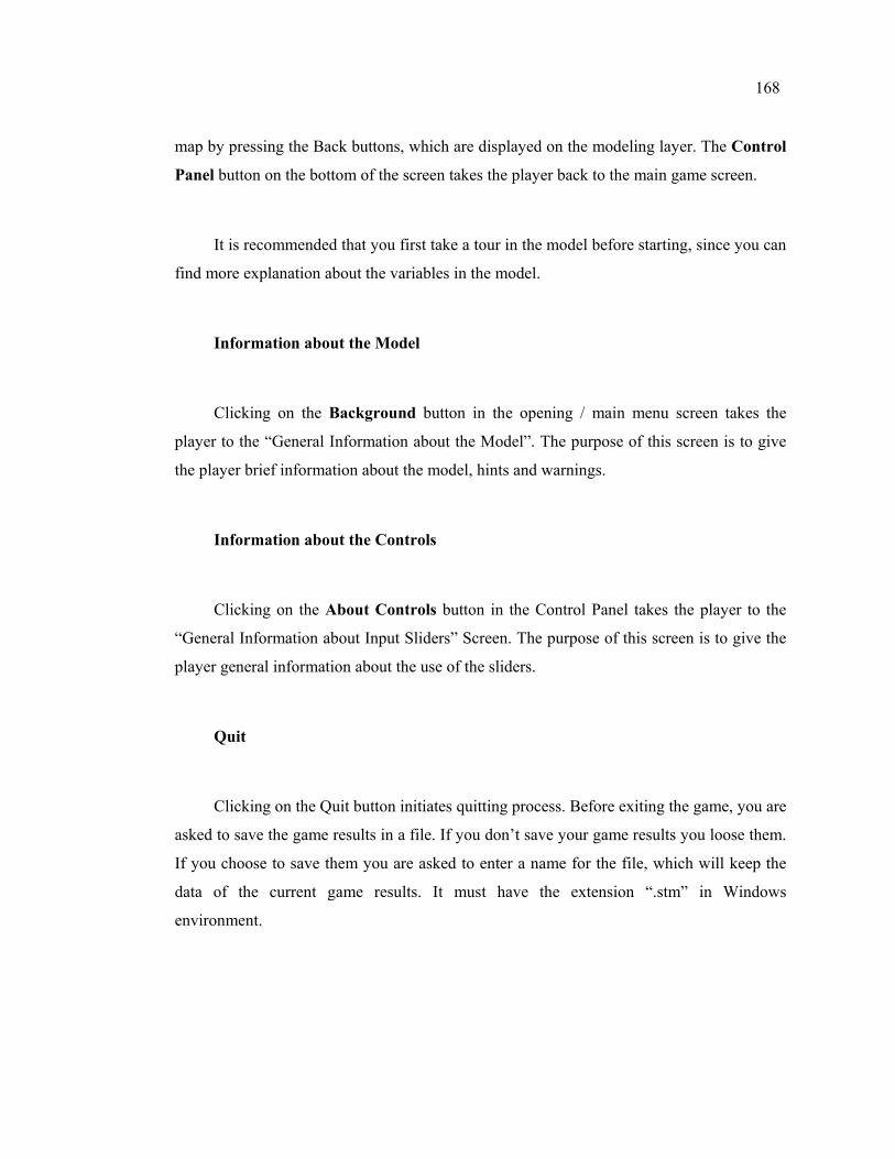
168
map by pressing the Back buttons, which are displayed on the modeling layer. The Control
Panel button on the bottom of the screen takes the player back to the main game screen.
It is recommended that you first take a tour in the model before starting, since you can
find more explanation about the variables in the model.
Information about the Model
Clicking on the Background button in the opening / main menu screen takes the
player to the “General Information about the Model”. The purpose of this screen is to give
the player brief information about the model, hints and warnings.
Information about the Controls
Clicking on the About Controls button in the Control Panel takes the player to the
“General Information about Input Sliders” Screen. The purpose of this screen is to give the
player general information about the use of the sliders.
Quit
Clicking on the Quit button initiates quitting process. Before exiting the game, you are
asked to save the game results in a file. If you don’t save your game results you loose them.
If you choose to save them you are asked to enter a name for the file, which will keep the
data of the current game results. It must have the extension “.stm” in Windows
environment.
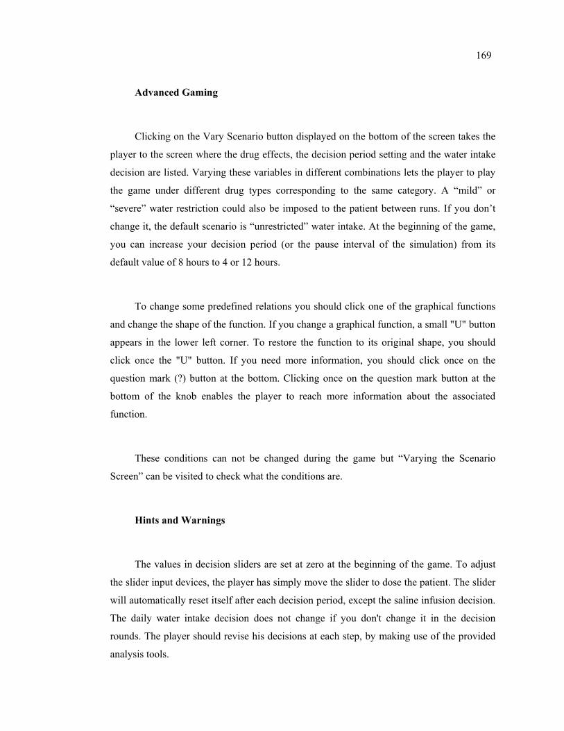
169
Advanced Gaming
Clicking on the Vary Scenario button displayed on the bottom of the screen takes the
player to the screen where the drug effects, the decision period setting and the water intake
decision are listed. Varying these variables in different combinations lets the player to play
the game under different drug types corresponding to the same category. A “mild” or
“severe” water restriction could also be imposed to the patient between runs. If you don’t
change it, the default scenario is “unrestricted” water intake. At the beginning of the game,
you can increase your decision period (or the pause interval of the simulation) from its
default value of 8 hours to 4 or 12 hours.
To change some predefined relations you should click one of the graphical functions
and change the shape of the function. If you change a graphical function, a small "U" button
appears in the lower left corner. To restore the function to its original shape, you should
click once the "U" button. If you need more information, you should click once on the
question mark (?) button at the bottom. Clicking once on the question mark button at the
bottom of the knob enables the player to reach more information about the associated
function.
These conditions can not be changed during the game but “Varying the Scenario
Screen” can be visited to check what the conditions are.
Hints and Warnings
The values in decision sliders are set at zero at the beginning of the game. To adjust
the slider input devices, the player has simply move the slider to dose the patient. The slider
will automatically reset itself after each decision period, except the saline infusion decision.
The daily water intake decision does not change if you don't change it in the decision
rounds. The player should revise his decisions at each step, by making use of the provided
analysis tools.
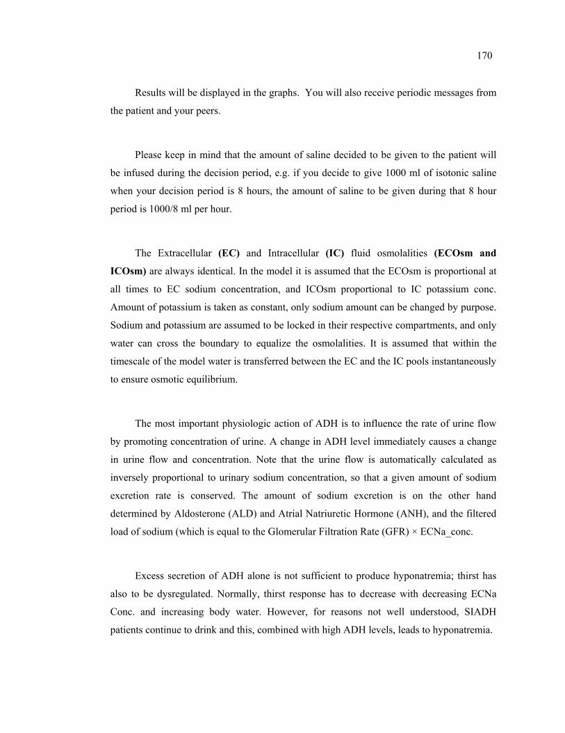
170
Results will be displayed in the graphs. You will also receive periodic messages from
the patient and your peers.
Please keep in mind that the amount of saline decided to be given to the patient will
be infused during the decision period, e.g. if you decide to give 1000 ml of isotonic saline
when your decision period is 8 hours, the amount of saline to be given during that 8 hour
period is 1000/8 ml per hour.
The Extracellular (EC) and Intracellular (IC) fluid osmolalities (ECOsm and
ICOsm) are always identical. In the model it is assumed that the ECOsm is proportional at
all times to EC sodium concentration, and ICOsm proportional to IC potassium conc.
Amount of potassium is taken as constant, only sodium amount can be changed by purpose.
Sodium and potassium are assumed to be locked in their respective compartments, and only
water can cross the boundary to equalize the osmolalities. It is assumed that within the
timescale of the model water is transferred between the EC and the IC pools instantaneously
to ensure osmotic equilibrium.
The most important physiologic action of ADH is to influence the rate of urine flow
by promoting concentration of urine. A change in ADH level immediately causes a change
in urine flow and concentration. Note that the urine flow is automatically calculated as
inversely proportional to urinary sodium concentration, so that a given amount of sodium
excretion rate is conserved. The amount of sodium excretion is on the other hand
determined by Aldosterone (ALD) and Atrial Natriuretic Hormone (ANH), and the filtered
load of sodium (which is equal to the Glomerular Filtration Rate (GFR) × ECNa_conc.
Excess secretion of ADH alone is not sufficient to produce hyponatremia; thirst has
also to be dysregulated. Normally, thirst response has to decrease with decreasing ECNa
Conc. and increasing body water. However, for reasons not well understood, SIADH
patients continue to drink and this, combined with high ADH levels, leads to hyponatremia.
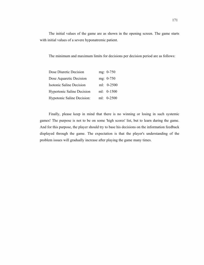
171
The initial values of the game are as shown in the opening screen. The game starts
with initial values of a severe hyponatremic patient.
The minimum and maximum limits for decisions per decision period are as follows:
Dose Diuretic Decision mg: 0-750
Dose Aquaretic Decision mg: 0-750
Isotonic Saline Decision ml: 0-2500
Hypertonic Saline Decision ml: 0-1500
Hypotonic Saline Decision: ml: 0-2500
Finally, please keep in mind that there is no winning or losing in such systemic
games! The purpose is not to be on some 'high scores' list, but to learn during the game.
And for this purpose, the player should try to base his decisions on the information feedback
displayed through the game. The expectation is that the player's understanding of the
problem issues will gradually increase after playing the game many times.
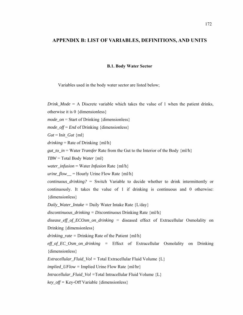
172
APPENDIX B: LIST OF VARIABLES, DEFINITIONS, AND UNITS
B.1. Body Water Sector
Variables used in the body water sector are listed below;
Drink_Mode = A Discrete variable which takes the value of 1 when the patient drinks,
otherwise it is 0 {dimensionless}
mode_on = Start of Drinking {dimensionless}
mode_off = End of Drinking {dimensionless}
Gut = Init_Gut {ml}
drinking = Rate of Drinking {ml/h}
gut_to_in = Water Transfer Rate from the Gut to the Interior of the Body {ml/h}
TBW = Total Body Water {ml}
water_infusion = Water Infusion Rate {ml/h}
urine_flow__ = Hourly Urine Flow Rate {ml/h}
continuous_drinking? = Switch Variable to decide whether to drink intermittently or
continuously. It takes the value of 1 if drinking is continuous and 0 otherwise:
{dimensionless}
Daily_Water_Intake = Daily Water Intake Rate {L/day}
discontinuous_drinking = Discontinuous Drinking Rate {ml/h}
disease_eff_of_ECOsm_on_drinking = diseased effect of Extracellular Osmolality on
Drinking {dimensionless}
drinking_rate = Drinking Rate of the Patient {ml/h}
eff_of_EC_Osm_on_drinking = Effect of Extracellular Osmolality on Drinking
{dimensionless}
Extracellular_Fluid_Vol = Total Extracellular Fluid Volume {L}
implied_UFlow = Implied Urine Flow Rate {ml/hr}
Intracellular_Fluid_Vol =Total Intracellular Fluid Volume {L}
key_off = Key-Off Variable {dimensionless}
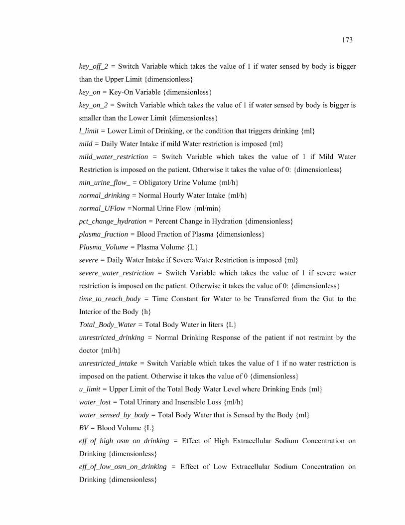
173
key_off_2 = Switch Variable which takes the value of 1 if water sensed by body is bigger
than the Upper Limit {dimensionless}
key_on = Key-On Variable {dimensionless}
key_on_2 = Switch Variable which takes the value of 1 if water sensed by body is bigger is
smaller than the Lower Limit {dimensionless}
l_limit = Lower Limit of Drinking, or the condition that triggers drinking {ml}
mild = Daily Water Intake if mild Water restriction is imposed {ml}
mild_water_restriction = Switch Variable which takes the value of 1 if Mild Water
Restriction is imposed on the patient. Otherwise it takes the value of 0: {dimensionless}
min_urine_flow_ = Obligatory Urine Volume {ml/h}
normal_drinking = Normal Hourly Water Intake {ml/h}
normal_UFlow =Normal Urine Flow {ml/min}
pct_change_hydration = Percent Change in Hydration {dimensionless}
plasma_fraction = Blood Fraction of Plasma {dimensionless}
Plasma_Volume = Plasma Volume {L}
severe = Daily Water Intake if Severe Water Restriction is imposed {ml}
severe_water_restriction = Switch Variable which takes the value of 1 if severe water
restriction is imposed on the patient. Otherwise it takes the value of 0: {dimensionless}
time_to_reach_body = Time Constant for Water to be Transferred from the Gut to the
Interior of the Body {h}
Total_Body_Water = Total Body Water in liters {L}
unrestricted_drinking = Normal Drinking Response of the patient if not restraint by the
doctor {ml/h}
unrestricted_intake = Switch Variable which takes the value of 1 if no water restriction is
imposed on the patient. Otherwise it takes the value of 0 {dimensionless}
u_limit = Upper Limit of the Total Body Water Level where Drinking Ends {ml}
water_lost = Total Urinary and Insensible Loss {ml/h}
water_sensed_by_body = Total Body Water that is Sensed by the Body {ml}
BV = Blood Volume {L}
eff_of_high_osm_on_drinking = Effect of High Extracellular Sodium Concentration on
Drinking {dimensionless}
eff_of_low_osm_on_drinking = Effect of Low Extracellular Sodium Concentration on
Drinking {dimensionless}
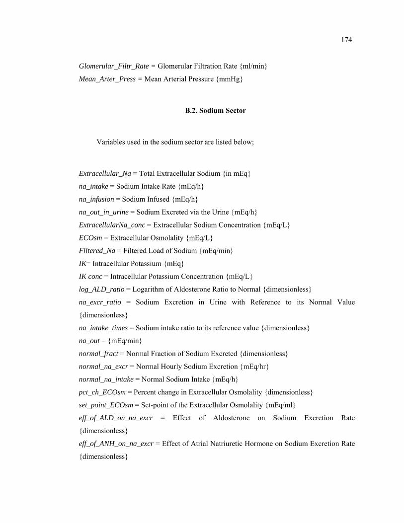
174
Glomerular_Filtr_Rate = Glomerular Filtration Rate {ml/min}
Mean_Arter_Press = Mean Arterial Pressure {mmHg}
B.2. Sodium Sector
Variables used in the sodium sector are listed below;
Extracellular_Na = Total Extracellular Sodium {in mEq}
na_intake = Sodium Intake Rate {mEq/h}
na_infusion = Sodium Infused {mEq/h}
na_out_in_urine = Sodium Excreted via the Urine {mEq/h}
ExtracellularNa_conc = Extracellular Sodium Concentration {mEq/L}
ECOsm = Extracellular Osmolality {mEq/L}
Filtered_Na = Filtered Load of Sodium {mEq/min}
IK= Intracellular Potassium {mEq}
IK conc = Intracellular Potassium Concentration {mEq/L}
log_ALD_ratio = Logarithm of Aldosterone Ratio to Normal {dimensionless}
na_excr_ratio = Sodium Excretion in Urine with Reference to its Normal Value
{dimensionless}
na_intake_times = Sodium intake ratio to its reference value {dimensionless}
na_out = {mEq/min}
normal_fract = Normal Fraction of Sodium Excreted {dimensionless}
normal_na_excr = Normal Hourly Sodium Excretion {mEq/hr}
normal_na_intake = Normal Sodium Intake {mEq/h}
pct_ch_ECOsm = Percent change in Extracellular Osmolality {dimensionless}
set_point_ECOsm = Set-point of the Extracellular Osmolality {mEq/ml}
eff_of_ALD_on_na_excr = Effect of Aldosterone on Sodium Excretion Rate
{dimensionless}
eff_of_ANH_on_na_excr = Effect of Atrial Natriuretic Hormone on Sodium Excretion Rate
{dimensionless}
175
B.3. Endocrine System Sector Group
Variables used in the Antidiuretic Hormone (ADH), Renin-Angiotensin-Aldosterone
System (RAAS) and the Atrial Natriuretic Hormone (ANH) subsectors are listed below;
ADH_in_plasma = Amount of Antidiuretic hormone in plasma {pg}
actual_ADH_release = Actual release of ADH from the pool {pg/h}
ADH_clear = Antidiuretic hormone clearance {pg/h}
ADH_Pool = Amount of ADH in the pool {pg}
ADH_production = ADH production rate {pg/h}
ADH_adj_time = ADH release adjustment time {h}
ADH_clear_del = Antidiuretic hormone clearance delay {h}
ADH_conc_in_plasma = Plasma Antidiuretic hormone concentration {pg/ml}
ADH_ratio_to_normal = Antidiuretic hormone concentration ratio with reference to its
normal {dimensionless}
desired_ADH_conc = Desired ADH concentration {pg/ml}
desired_ADH_release = Desired antidiuretic hormone release {pg/h}
des_ADH_in_plasma = Desired antidiuretic hormone in plasma {pg}
max_pool_cap = Maximum ADH pool capacity {pg}
normal_ADH_conc = Normal Antidiuretic hormone concentration in man {pg/ml}
normal_BV = Normal blood volume {L}
pct_chg_BV = Percent change in Blood volume {dimensionless}
pct_decrease_in_cap = Percent decrease in ADH pool capacity {dimensionless}
pool_capacity = ADH pool capacity {pg}
eff_of_ADH_avail = Effect of ADH availability in the pool {dimensionless}
eff_of_BV_on_ADH = effect of Blood Volume on ADH {dimensionless}
eff_of_ECOsm_on_ADH = effect of Extracellular Osmolality (ECOsm) on ADH
{dimensionless}
normal_PV = Normal Plasma Volume {L}
eff_of_cap_on_ADH_prod = Effect of Pool Capacity on ADH production {dimensionless}
normal_ADH_prod = Normal ADH Production Rate {pg/h}
176
ALD = Amount of aldosterone {ng}
ALD_adjust = Aldosterone adjustment rate {ng/h}
ALD_conc_perceived = Perceived aldosterone concentration in plasma {ng/dl}
ALD_correct = Perceived Aldosterone Concentration Correction Rate {ng/h}
Renin = Amount of renin {ng}
renin_secr = Renin Secretion Rate {ng/h}
ALD_adj_time = Aldosterone adjustment time {h}
ALD_conc = Aldosterone Concentration in Plasma {ng/dl}
ALD_conc_normal = Normal Aldosterone Concentration in Plasma {ng/dl}
ALD_conc_perceive_del = Aldosterone Concentration Perceive Delay {h}
ALD_ratio = Perceived Aldosterone Concentration with Referece to its Normal Value
{dimensionless}
ALD_ratio_to_normal = Aldosterone Concentration with Reference to its Normal
{dimensionless}
ANG_conc = Angiotensin Concentration {ng}
normal_TBW = Normal Value of Total Body Water {ml}
desired_ALD = Desired amount of aldosterone in body water {ng}
desired_ALD_conc = Desired aldosterone concentration {ng/dl}
desired_renin = Desired Renin Amount {ng}
desired_renin_activity = Desired Renin Activity {dimensionless}
log_ANG = Logarithm of Angiotensin Concentration {dimensionless}
normal_renin_activity = The Normal Renin Activity in Man {ng/L}
renin_del = Renin Delay {h}
renin_ratio = Renin Ratio to Normal {dimensionless}
eff_of_MAP_on_renin = Effect of Mean Arterial Pressure on Renin {dimensionless}
eff_of_ANG_on_ALD = Effect of Angiotensin on Aldosterone Secretion {dimensionless}
eff_of_ECNa_conc_on_ALD = Effect of Extracellular Sodium Concentration (ECNa Conc)
on Aldosterone Secretion {dimensionless}
ANH_in_plasma = Atrial Natriuretic Hormone in Plasma {ng}
ANH_production = Atrial Natriuretic Hormone Production {ng}
ANH_clear_del = Atrial Natriuretic Hormone Clearance Delay {h}
ANH_conc_in_plasma = Plasma Atrial Natriuretic Hormone Concentration {ng/L}
177
ANH_ratio_to_normal = Atrial Natriuretic Hormone Concentration with Reference to its
Normal Value {dimensionless}
basal_ANH_conc = Basal Atrial Natriuretic Hormone Concentration {ng/ml}
desired_ANH_conc = Desired Atrial Natriuretic Hormone Concentration {ng/l}
desired_ANH_in_plasma = Desired ANH in Plasma {ng}
eff_of_ANH_on_na_excr = Effect of Atrial Natriuretic Hormone on Sodium Excretion
{dimensionless}
eff_of_ANH = Effect of Atrial Natriuretic Hormone on Sodium Excretion {dimensionless}
eff_of_ECFV_on_ANH = Effect of Percent Change in Extracellular Fluid Volume on Atrial
Natriuretic Hormone {dimensionless}
eff_of_ecf_icf_ratio_on_ANH = Effect of ECF/ICF ratio on Atrial Natriuretic Hormone
{dimensionless}
ecf_over_icf = Extracellular-intracellular fluid volume ratio {dimensionless}
normal_ECFV = Normal value of Extracelular Fluid Volume {L}
pct_chg_ECFV: Percent change in Extracellular fluid volume {dimensionless}
B.4. Urinary Sodium Concentration Sector
Variables used in the Urinary Sodium Concentration sector are listed below;
implied_UNa_conc = Implied Urinary Sodium Concentration {mEq/L}
implied_UNa_conc_by_ADH = Implied Urinary Sodium Concentration by ADH {mEq/l}
max_att_UNa_conc = Maximum Attainable Urinary Sodium Concentration {mEq/L}
max_UNa_conc = Maximum Urinary Sodium Concentration that the Human Kidney can
Attain {mEq/L}
min_UNa_conc = Minimum Urinary Sodium Concentration that the Human Kidney can
Attain {mEq/L}
GFRo = Normal Value of the Gloerular Filtration Rate {ml/min}
normal_UNa_conc = Normal Urinary Sodium Concentration in Man {mEq/L}
178
potential_escape = Potential Escape from Effects of High Circulating Levels of ADH
{dimensionless}
prc_chg_GFR = Percent Change in Glomerular Filtration Rate {dimensionless}
Urinary_Na_conc = Urinary Sodium Concentration {mEq/L}
eff_of_GFR_on_UNa = Effect of GFR on Urinary Sodium Concentration {dimensionless}
eff_of_max_att_UNa_on_UNa = Effect of Maximum Attainable Urinary Sodium
Concentration on Urinary Sodium Concentration {dimensionless}
escape = Escape from Effects of High Circulating Levels of ADH {dimensionless}
eff_of_ADH = Effect of Antidiuretic Hormone to Urinary Sodium Concentration
{dimensionless}
B.5. Treatment Sector Group
Variables used in the Diuretic, Aquaretic and Intravenous Fluid Infusion (Intr. Fluid
Inf) subsectors are listed below;
Diuretic_in_Blood = Amount of Active Diuretic in Blood {mg}
intravenous_diuretic = Diuretic Given to the Bloodstream {mg/DT}
diuretic_absorption = Diuretic Absorption {mg/h}
clear_diuretic = Clearance of Diuretic {mg/h}
Diuretic_in_Stomach = Amount of Diuretic in Stomach {mg}
oral_diuretic = Oral Diuretic Given {mg/DT}
diuretic_absorption = Diuretic Absorption {mg/h}
Perceived_Diuretic_conc = Perceived Diuretic Concentration in Plasma {mg}
correct_diuretic_conc = Correction of Perceived Diuretic Concentration {mg/L/h}
diuretic_abs_const = Diuretic Absorption Constant: the Exponential Time Constant
Associated with the Absorption Half-life {1/h}
diuretic_blood_conc = Diuretic Concentration in Blood: This converter calculates the
concentration of the drug in the bloodstream. {mg/L}
diuretic_clear_del = Diuretic Clearance Delay {h}
diuretic_del = Diuretic Delay {h}
diuretic_stomach_conc = Diuretic Stomach Concentration {mg/L}
179
DOSE_DIURETIC = Dose of Diuretic Given {mg}
Intravenous_Dose_Diuretic = Intravenous Dose Diuretic {mg}
Oral_Dose_Diuretic = Oral Dose Diuretic {mg}
eff_of_diuretic_on_na_excr = Effect of Diuretic on Sodium Excretion {dimensionless}
eff_of_diuretic_on_UNa = Effect of Diuretic on Urinary Sodium Concentration
{dimensionless}
Aquaretic_in_Blood = Amount of Active Aquaretic (or Antidiuretic Hormone (ADH)
antagonist) in Blood {mg}
intravenous_aquaretic = Aquaretic Given to the Bloodstream {mg/DT}
aquaretic_absorption = Aquaretic Absorption {mg/h}
clear_aquaretic = Clearance of Aquaretic {mg/h}
Aquaretic_in_Stomach = Aquaretic in Stomach {mg}
oral_aquaretic = Oral Aquaretic Given {mg/h}
aquaretic_absorption = Aquaretic Absorption {mg/h}
Perceived_Aquaretic_conc = Perceived Aquaretic Concentration {mg/L}
correct_aquaretic_conc = Correction of Perceived Aquaretic Concentration {mg/L/h}
aquaretic_clear_del = ADH Antagonist (Aquaretic} Clearance Delay {h}
aquaretic_abs_const = Aquaretic Absorption Constant: the exponential time constant
associated with the absorption half-life. {1/h}
aquaretic_blood_conc = Aquaretic Concentration in Blood {mg/L}
aquaretic_del = Aquaretic Delay {h}
aquaretic_stomach_conc = Aquaretic Stomach Volume {mg/L}
DOSE_ADH_ANTAGONIST = Dose of Aquaretic Given {mg}
intravenous = {dimensionless}
Intravenous_Dose_Aquaretic = Intravenous Dose Aquaretic {mg}
Oral_Dose_Aquaretic = Oral Dose Aquaretic {mg}
stomach_volume = Stomach Volume {L}
eff_of_aquaretic_on_ADH = Effect of Aquaretic on Antidiuretic Hormone (ADH)
{dimensionless}
eff_of_aquaretic_on_UNa = Effect of Aquaretic on Urinary Sodium Concentration:
{dimensionless}
180
Sodium_Load_Given = Total Sodium Load Given in the Course of Treatment {mEq}
na_in = Infused Sodium {mEq/h}
Water_Load_given = Total Water Load Given in the Course of Treatment {ml}
water_in = Infused Water {ml/h}
HYPERTONIC_3%_SALINE = Hypertonic Saline Infused to the Patient: Hypertonic saline
3% has an osmolality (about 900 mosm/l) three times that of plasma {ml/h}
HYPOTONIC_SALINE = Hypotonic Saline Infused to the Patient: Hypotonic solutions vary
between 0.45% and 0, 18 % saline (77 and 30 mEq/L Na). They have an osmolality smaller
than the normal plasma osmolality {ml/h}
ISOTONIC_SALINE = Isotonic Saline Infused to the Patient: Isotonic saline is 0,9% saline
(142 mEq/L Na). This solution has an [Na+] similar to that of the extracellular fluid which
effectively limits its fluid distribution to the ECF{ml/h}
na_infused = Amount of Sodium Infused to the Patient {mEq/h}
water_infused = Amount of Water Infused to the Patient {ml/h}
B.6. Game Related-Not in a Sector
Variables which do not belong to any sector, but rather used for the game purposes,
are listed below;
Na_In_Current_Period = Total Amount of Sodium given to the Patient in the Current
Period {mEq}
na_intake_period = Total Sodium Intake Rate of the Patient {mEq/h}
na_out_period = Total Sodium Loss Rate of the Patient {mEq/h}
Na_Out_Current_Period = Total Sodium Lost by the Patient in the Current Period {mEq}
na_lost_period = Sodium Loss Rate in Urine {mEq/h}
na_lost_out_period = Reset the Stock of the Current Sodium Loss {Eq/h}
Total_Change_in_ECNa_conc = Total Change in Extracellular Sodium Concentration
{mEq/L}
rate_of_change = Rate of Change in ECNa Concentration {mEq/L/h}
Urine_Output_Current_Period = Total Urine Collected, which takes the value of 0 between
measurements {L}
181
UFlow_in_period = Hourly Urine Flow {ml/h}
UFlow_out_period = Reset the Current Urine Stock {ml/h}
Urine_Period = Amount of Urine of the Corresponding Period {ml}
urine_flow [1] = Urine Flow of the First Period {ml/h}
…….
urine_flow [30] = Urine Flow of the Thirtieth Period {ml/h}
WaterInPeriod= Amount of Water Intake of the Corresponding Period {ml}
fluid_intake [1] = Water Intake Rate of the First Period {ml/h}
……..
fluid_intake [30] = Water Intake Rate of the Thirtieth Period {ml/h}
Water_Intake_Current_Period = Total Amount of Water Given to the Patient in the Current
Decision Period {ml}
water_out_period = Reset the Stock of the Current Water Intake {ml/h}
Aldosterone_Ratio_to_Normal = Aldosterone Ratio to Normal, which takes the value of 0
between measurements {dimensionless}
Antidiuretic_Hormone_Ratio_to_Normal = ADH Ratio to Normal, which takes the value of
0 between measurements {dimensionless}
Atrial_Natriuretic_Hormone_Ratio_to_Normal = ANH Ratio to Normal, which takes the
value of 0 between measurements {dimensionless}
bedside_attendant = Messages of the Bedside Attendant related to ECNa Concentration
{dimensionless}
Body_Water_\_L = Amount of TBW, which takes the value of 0 between measurements
{L}
cumulative_interval = Current Time Period {dimensionless}
Daily_ECNa_correct = Absolute Rate of Daily Change in ECNa Concentration {mEq/L}
Daily_ECNa_Correction_Rate = Daily Correction Rate of ECNa Concentration, which
takes the value of 0 between measurements {mEq/L/d}
Daily_ECNa_Corr_Lower_Limit = Lower Limit of Daily ECNa Correction Rate
{mEq/L/d}
Daily_ECNa_Corr_Upper_Limit = Upper Limit of Daily ECNa Correction Rate
{mEq/L/d}
Daily_Fluid_Intake = Dummy Converter for Daily Water Intake
decision_period = "Pause Interval" of the Simulation {h}
182
dec_variable_period = A variable which takes the value of 1 on the multiples of the
selected decision period, and takes the value of 0 otherwise {dimensionless}
Drug_Dosage_Given = Dummy Converter for the Given Drug Dosage {mg}
ECNa_conc_an_hour = Extracellular Sodium Concentration Delayed One Hour {mEq/L}
ECNa_conc_daily = Extracellular Sodium Concentration Delayed One Day {mEq/L}
ECNa_correction = Absolute Rate of Hourly Change in ECNa Concentration {mEq/L}
eight_hours = Switch variable which takes the value of 1 if 8 hours is selected as the
decision period {dimensionless}
Estimated_Insensible_Loss_in_that_Period_\_L = Insensible Loss of the Decision Period
{L}
Extracellular_Fluid_Volume_\_L = Extracellular Fluid Volume, which takes the value of 0
between measurements {L}
Extracellular_Sodium_Concentration\_mEq\L = Extracellular Sodium Concentration,
which takes the value of 0 between measurements {mEq/L}
Extracellular_Sodium_\_mEq = Amount of Extracellular Sodium, which takes the value of
0 between measurements {mEq}
four_hours = Switch variable which takes the value of 1 if 4 hours is selected as the
decision period {dimensionless}
Glomerular_Filtration_Rate_\_ml\min = Glomerular Filtration Rate, which takes the value
of 0 between measurements {ml/min}
heaven = Message from heaven when the patient dies due to low ECNa concentration
{dimensionless}
heaven2 = Message from heaven when the patient dies due to high blood pressure
{dimensionless}
Hourly_ECNa_Correction_Rate = Hourly Correction Rate of ECNa concentration, which
takes the value of 0 between measurements {mEq/L/h}
Hourly_ECNa_Corr_Lower_Limit = Lower limit for Hourly Correction Rate of ECNa
Concentration {mEq/L/h}
Hourly_ECNa_Corr_Upper_Limit = Upper Limit for Hourly Correction Rate of ECNa
Concentration {mEq/L/h} {mEq/L/h}
Init_ADH = Initial Value of Antidiuretic Hormone in Plasma for the Game {pg}
Init_ADH_Pool = Initial Value of Antidiuretic Hormone Pool for the Game {pg}
Init_ALD = Initial Value of Aldosterone for the Game {ng}
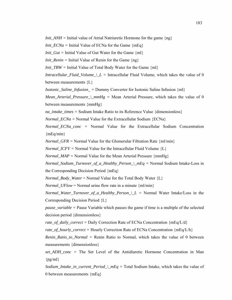
183
Init_ANH = Initial value of Atrial Natriuretic Hormone for the game {ng}
Init_ECNa = Initial Value of ECNa for the Game {mEq}
Init_Gut = Initial Value of Gut Water for the Game {ml}
Init_Renin = Initial Value of Renin for the Game {ng}
Init_TBW = Initial Value of Total Body Water for the Game {ml}
Intracellular_Fluid_Volume_\_L = Intracellular Fluid Volume, which takes the value of 0
between measurements {L}
Isotonic_Saline_Infusion_ = Dummy Converter for Isotonic Saline Infusion {ml}
Mean_Arterial_Pressure_\_mmHg = Mean Arterial Pressure, which takes the value of 0
between measurements {mmHg}
na_intake_times = Sodium Intake Ratio to its Reference Value {dimensionless}
Normal_ECNa = Normal Value for the Extracellular Sodium {ECNa}
Normal_ECNa_conc = Normal Value for the Extracellular Sodium Concentration
{mEq/min}
Normal_GFR = Normal Value for the Glomerular Filtration Rate {ml/min}
Normal_ICFV = Normal Value for the Intracellular Fluid Volume {L}
Normal_MAP = Normal Value for the Mean Arterial Pressure {mmHg}
Normal_Sodium_Turnover_of_a_Healthy_Person_\_mEq = Normal Sodium Intake-Loss in
the Corresponding Decision Period {mEq}
Normal_Body_Water = Normal Value for the Total Body Water {L}
Normal_UFlow = Normal urine flow rate in a minute {ml/min}
Normal_Water_Turnover_of_a_Healthy_Person_\_L = Normal Water Intake/Loss in the
Corresponding Decision Period {L}
pause_variable = Pause Variable which pauses the game if time is a multiple of the selected
decision period {dimensionless}
rate_of_daily_correct = Daily Correction Rate of ECNa Concentration {mEq/L/d}
rate_of_hourly_correct = Hourly Correction Rate of ECNa Concentration {mEq/L/h}
Renin_Ratio_to_Normal = Renin Ratio to Normal, which takes the value of 0 between
measurements {dimensionless}
set_ADH_conc = The Set Level of the Antidiuretic Hormone Concentration in Man
{pg/ml}
Sodium_Intake_in_current_Period_\_mEq = Total Sodium Intake, which takes the value of
0 between measurements {mEq}
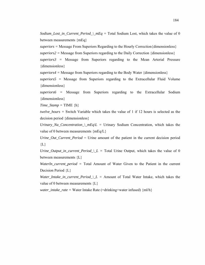
184
Sodium_Lost_in_Current_Period_\_mEq = Total Sodium Lost, which takes the value of 0
between measurements {mEq}
superiors = Message From Superiors Regarding to the Hourly Correction{dimensionless}
superiors2 = Message from Superiors regarding to the Daily Correction {dimensionless}
superiors3 = Message from Superiors regarding to the Mean Arterial Pressure
{dimensionless}
superiors4 = Message from Superiors regarding to the Body Water {dimensionless}
superiors5 = Message from Superiors regarding to the Extracellular Fluid Volume
{dimensionless}
superiors6 = Message from Superiors regarding to the Extracellular Sodium
{dimensionless}
Time_Stamp = TIME {h}
twelve_hours = Switch Variable which takes the value of 1 if 12 hours is selected as the
decision period {dimensionless}
Urinary_Na_Concentration_\_mEq\L = Urinary Sodium Concentration, which takes the
value of 0 between measurements {mEq/L}
Urine_Out_Current_Period = Urine amount of the patient in the current decision period
{L}
Urine_Output_in_current_Period_\_L = Total Urine Output, which takes the value of 0
between measurements {L}
WaterIn_current_period = Total Amount of Water Given to the Patient in the current
Decision Period {L}
Water_Intake_in_current_Period_\_L = Amount of Total Water Intake, which takes the
value of 0 between measurements {L}
water_intake_rate = Water Intake Rate (=drinking+water infused) {ml/h}
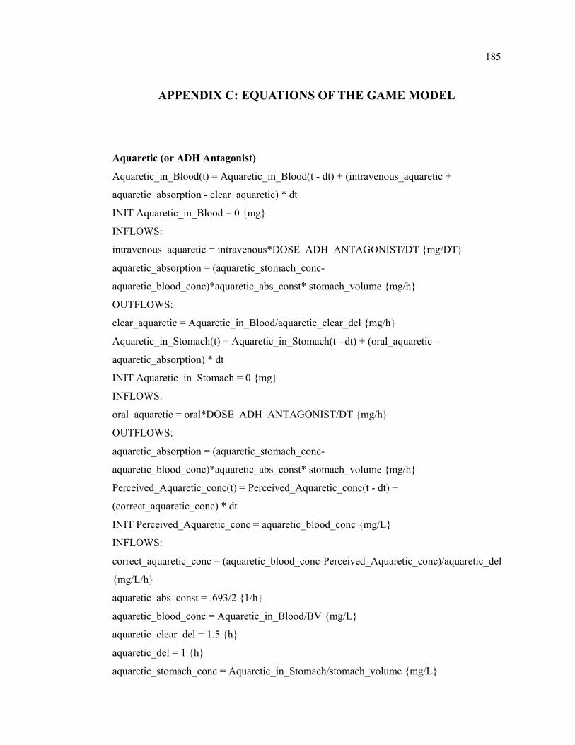
185
APPENDIX C: EQUATIONS OF THE GAME MODEL
Aquaretic (or ADH Antagonist)
Aquaretic_in_Blood(t) = Aquaretic_in_Blood(t - dt) + (intravenous_aquaretic +
aquaretic_absorption - clear_aquaretic) * dt
INIT Aquaretic_in_Blood = 0 {mg}
INFLOWS:
intravenous_aquaretic = intravenous*DOSE_ADH_ANTAGONIST/DT {mg/DT}
aquaretic_absorption = (aquaretic_stomach_conc-
aquaretic_blood_conc)*aquaretic_abs_const* stomach_volume {mg/h}
OUTFLOWS:
clear_aquaretic = Aquaretic_in_Blood/aquaretic_clear_del {mg/h}
Aquaretic_in_Stomach(t) = Aquaretic_in_Stomach(t - dt) + (oral_aquaretic -
aquaretic_absorption) * dt
INIT Aquaretic_in_Stomach = 0 {mg}
INFLOWS:
oral_aquaretic = oral*DOSE_ADH_ANTAGONIST/DT {mg/h}
OUTFLOWS:
aquaretic_absorption = (aquaretic_stomach_conc-
aquaretic_blood_conc)*aquaretic_abs_const* stomach_volume {mg/h}
Perceived_Aquaretic_conc(t) = Perceived_Aquaretic_conc(t - dt) +
(correct_aquaretic_conc) * dt
INIT Perceived_Aquaretic_conc = aquaretic_blood_conc {mg/L}
INFLOWS:
correct_aquaretic_conc = (aquaretic_blood_conc-Perceived_Aquaretic_conc)/aquaretic_del
{mg/L/h}
aquaretic_abs_const = .693/2 {1/h}
aquaretic_blood_conc = Aquaretic_in_Blood/BV {mg/L}
aquaretic_clear_del = 1.5 {h}
aquaretic_del = 1 {h}
aquaretic_stomach_conc = Aquaretic_in_Stomach/stomach_volume {mg/L}
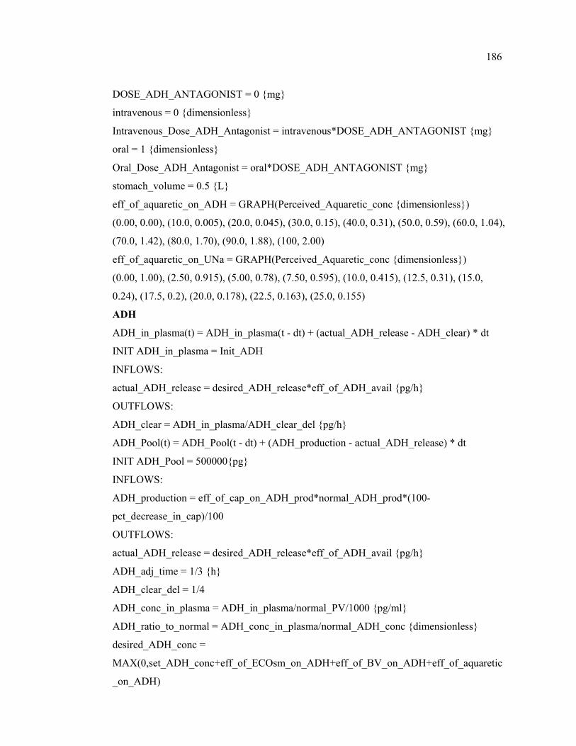
186
DOSE_ADH_ANTAGONIST = 0 {mg}
intravenous = 0 {dimensionless}
Intravenous_Dose_ADH_Antagonist = intravenous*DOSE_ADH_ANTAGONIST {mg}
oral = 1 {dimensionless}
Oral_Dose_ADH_Antagonist = oral*DOSE_ADH_ANTAGONIST {mg}
stomach_volume = 0.5 {L}
eff_of_aquaretic_on_ADH = GRAPH(Perceived_Aquaretic_conc {dimensionless})
(0.00, 0.00), (10.0, 0.005), (20.0, 0.045), (30.0, 0.15), (40.0, 0.31), (50.0, 0.59), (60.0, 1.04),
(70.0, 1.42), (80.0, 1.70), (90.0, 1.88), (100, 2.00)
eff_of_aquaretic_on_UNa = GRAPH(Perceived_Aquaretic_conc {dimensionless})
(0.00, 1.00), (2.50, 0.915), (5.00, 0.78), (7.50, 0.595), (10.0, 0.415), (12.5, 0.31), (15.0,
0.24), (17.5, 0.2), (20.0, 0.178), (22.5, 0.163), (25.0, 0.155)
ADH
ADH_in_plasma(t) = ADH_in_plasma(t - dt) + (actual_ADH_release - ADH_clear) * dt
INIT ADH_in_plasma = Init_ADH
INFLOWS:
actual_ADH_release = desired_ADH_release*eff_of_ADH_avail {pg/h}
OUTFLOWS:
ADH_clear = ADH_in_plasma/ADH_clear_del {pg/h}
ADH_Pool(t) = ADH_Pool(t - dt) + (ADH_production - actual_ADH_release) * dt
INIT ADH_Pool = 500000{pg}
INFLOWS:
ADH_production = eff_of_cap_on_ADH_prod*normal_ADH_prod*(100-
pct_decrease_in_cap)/100
OUTFLOWS:
actual_ADH_release = desired_ADH_release*eff_of_ADH_avail {pg/h}
ADH_adj_time = 1/3 {h}
ADH_clear_del = 1/4
ADH_conc_in_plasma = ADH_in_plasma/normal_PV/1000 {pg/ml}
ADH_ratio_to_normal = ADH_conc_in_plasma/normal_ADH_conc {dimensionless}
desired_ADH_conc =
MAX(0,set_ADH_conc+eff_of_ECOsm_on_ADH+eff_of_BV_on_ADH+eff_of_aquaretic
_on_ADH)
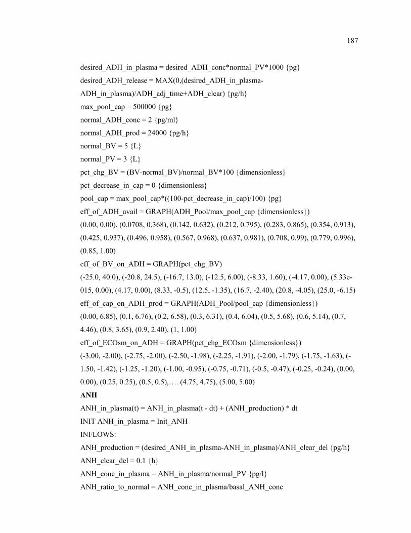
187
desired_ADH_in_plasma = desired_ADH_conc*normal_PV*1000 {pg}
desired_ADH_release = MAX(0,(desired_ADH_in_plasma-
ADH_in_plasma)/ADH_adj_time+ADH_clear) {pg/h}
max_pool_cap = 500000 {pg}
normal_ADH_conc = 2 {pg/ml}
normal_ADH_prod = 24000 {pg/h}
normal_BV = 5 {L}
normal_PV = 3 {L}
pct_chg_BV = (BV-normal_BV)/normal_BV*100 {dimensionless}
pct_decrease_in_cap = 0 {dimensionless}
pool_cap = max_pool_cap*((100-pct_decrease_in_cap)/100) {pg}
eff_of_ADH_avail = GRAPH(ADH_Pool/max_pool_cap {dimensionless})
(0.00, 0.00), (0.0708, 0.368), (0.142, 0.632), (0.212, 0.795), (0.283, 0.865), (0.354, 0.913),
(0.425, 0.937), (0.496, 0.958), (0.567, 0.968), (0.637, 0.981), (0.708, 0.99), (0.779, 0.996),
(0.85, 1.00)
eff_of_BV_on_ADH = GRAPH(pct_chg_BV)
(-25.0, 40.0), (-20.8, 24.5), (-16.7, 13.0), (-12.5, 6.00), (-8.33, 1.60), (-4.17, 0.00), (5.33e-
015, 0.00), (4.17, 0.00), (8.33, -0.5), (12.5, -1.35), (16.7, -2.40), (20.8, -4.05), (25.0, -6.15)
eff_of_cap_on_ADH_prod = GRAPH(ADH_Pool/pool_cap {dimensionless})
(0.00, 6.85), (0.1, 6.76), (0.2, 6.58), (0.3, 6.31), (0.4, 6.04), (0.5, 5.68), (0.6, 5.14), (0.7,
4.46), (0.8, 3.65), (0.9, 2.40), (1, 1.00)
eff_of_ECOsm_on_ADH = GRAPH(pct_chg_ECOsm {dimensionless})
(-3.00, -2.00), (-2.75, -2.00), (-2.50, -1.98), (-2.25, -1.91), (-2.00, -1.79), (-1.75, -1.63), (-
1.50, -1.42), (-1.25, -1.20), (-1.00, -0.95), (-0.75, -0.71), (-0.5, -0.47), (-0.25, -0.24), (0.00,
0.00), (0.25, 0.25), (0.5, 0.5),…. (4.75, 4.75), (5.00, 5.00)
ANH
ANH_in_plasma(t) = ANH_in_plasma(t - dt) + (ANH_production) * dt
INIT ANH_in_plasma = Init_ANH
INFLOWS:
ANH_production = (desired_ANH_in_plasma-ANH_in_plasma)/ANH_clear_del {pg/h}
ANH_clear_del = 0.1 {h}
ANH_conc_in_plasma = ANH_in_plasma/normal_PV {pg/l}
ANH_ratio_to_normal = ANH_conc_in_plasma/basal_ANH_conc
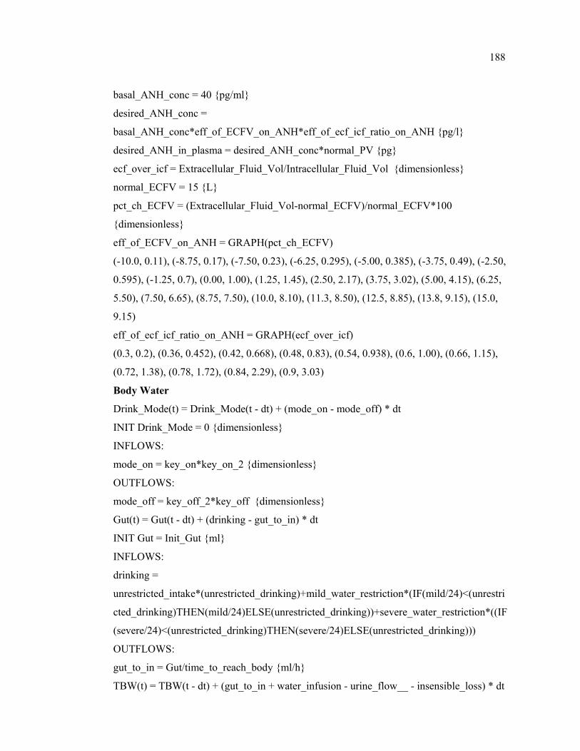
188
basal_ANH_conc = 40 {pg/ml}
desired_ANH_conc =
basal_ANH_conc*eff_of_ECFV_on_ANH*eff_of_ecf_icf_ratio_on_ANH {pg/l}
desired_ANH_in_plasma = desired_ANH_conc*normal_PV {pg}
ecf_over_icf = Extracellular_Fluid_Vol/Intracellular_Fluid_Vol {dimensionless}
normal_ECFV = 15 {L}
pct_ch_ECFV = (Extracellular_Fluid_Vol-normal_ECFV)/normal_ECFV*100
{dimensionless}
eff_of_ECFV_on_ANH = GRAPH(pct_ch_ECFV)
(-10.0, 0.11), (-8.75, 0.17), (-7.50, 0.23), (-6.25, 0.295), (-5.00, 0.385), (-3.75, 0.49), (-2.50,
0.595), (-1.25, 0.7), (0.00, 1.00), (1.25, 1.45), (2.50, 2.17), (3.75, 3.02), (5.00, 4.15), (6.25,
5.50), (7.50, 6.65), (8.75, 7.50), (10.0, 8.10), (11.3, 8.50), (12.5, 8.85), (13.8, 9.15), (15.0,
9.15)
eff_of_ecf_icf_ratio_on_ANH = GRAPH(ecf_over_icf)
(0.3, 0.2), (0.36, 0.452), (0.42, 0.668), (0.48, 0.83), (0.54, 0.938), (0.6, 1.00), (0.66, 1.15),
(0.72, 1.38), (0.78, 1.72), (0.84, 2.29), (0.9, 3.03)
Body Water
Drink_Mode(t) = Drink_Mode(t - dt) + (mode_on - mode_off) * dt
INIT Drink_Mode = 0 {dimensionless}
INFLOWS:
mode_on = key_on*key_on_2 {dimensionless}
OUTFLOWS:
mode_off = key_off_2*key_off {dimensionless}
Gut(t) = Gut(t - dt) + (drinking - gut_to_in) * dt
INIT Gut = Init_Gut {ml}
INFLOWS:
drinking =
unrestricted_intake*(unrestricted_drinking)+mild_water_restriction*(IF(mild/24)<(unrestri
cted_drinking)THEN(mild/24)ELSE(unrestricted_drinking))+severe_water_restriction*((IF
(severe/24)<(unrestricted_drinking)THEN(severe/24)ELSE(unrestricted_drinking)))
OUTFLOWS:
gut_to_in = Gut/time_to_reach_body {ml/h}
TBW(t) = TBW(t - dt) + (gut_to_in + water_infusion - urine_flow__ - insensible_loss) * dt
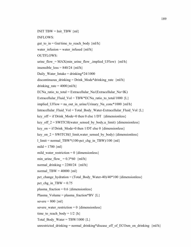
189
INIT TBW = Init_TBW {ml}
INFLOWS:
gut_to_in = Gut/time_to_reach_body {ml/h}
water_infusion = water_infused {ml/h}
OUTFLOWS:
urine_flow_= MAX(min_urine_flow_,implied_UFlow) {ml/h}
insensible_loss = 840/24 {ml/h}
Daily_Water_Intake = drinking*24/1000
discontinuous_drinking = Drink_Mode*drinking_rate {ml/h}
drinking_rate = 4000{ml/h}
ECNa_ratio_to_total = Extracellular_Na/(Extracellular_Na+IK)
Extracellular_Fluid_Vol = TBW*ECNa_ratio_to_total/1000 {L}
implied_UFlow = na_out_in_urine/Urinary_Na_conc*1000 {ml/h}
Intracellular_Fluid_Vol = Total_Body_Water-Extracellular_Fluid_Vol {L}
key_off = if Drink_Mode=0 then 0 else 1/DT {dimensionless}
key_off_2 = SWITCH(water_sensed_by_body,u_limit) {dimensionless}
key_on = if Drink_Mode=0 then 1/DT else 0 {dimensionless}
key_on_2 = SWITCH(l_limit,water_sensed_by_body) {dimensionless}
l_limit = normal_TBW*(100-pct_chg_in_TBW)/100 {ml}
mild = 1700 {ml}
mild_water_restriction = 0 {dimensionless}
min_urine_flow_ = 0.3*60 {ml/h}
normal_drinking = 2280/24 {ml/h}
normal_TBW = 40000 {ml}
pct_change_hydration = (Total_Body_Water-40)/40*100 {dimensionless}
pct_chg_in_TBW = 0.75
plasma_fraction = 0.6 {dimensionless}
Plasma_Volume = plasma_fraction*BV {L}
severe = 800 {ml}
severe_water_restriction = 0 {dimensionless}
time_to_reach_body = 1/2 {h}
Total_Body_Water = TBW/1000 {L}
unrestricted_drinking = normal_drinking*disease_eff_of_ECOsm_on_drinking {ml/h}
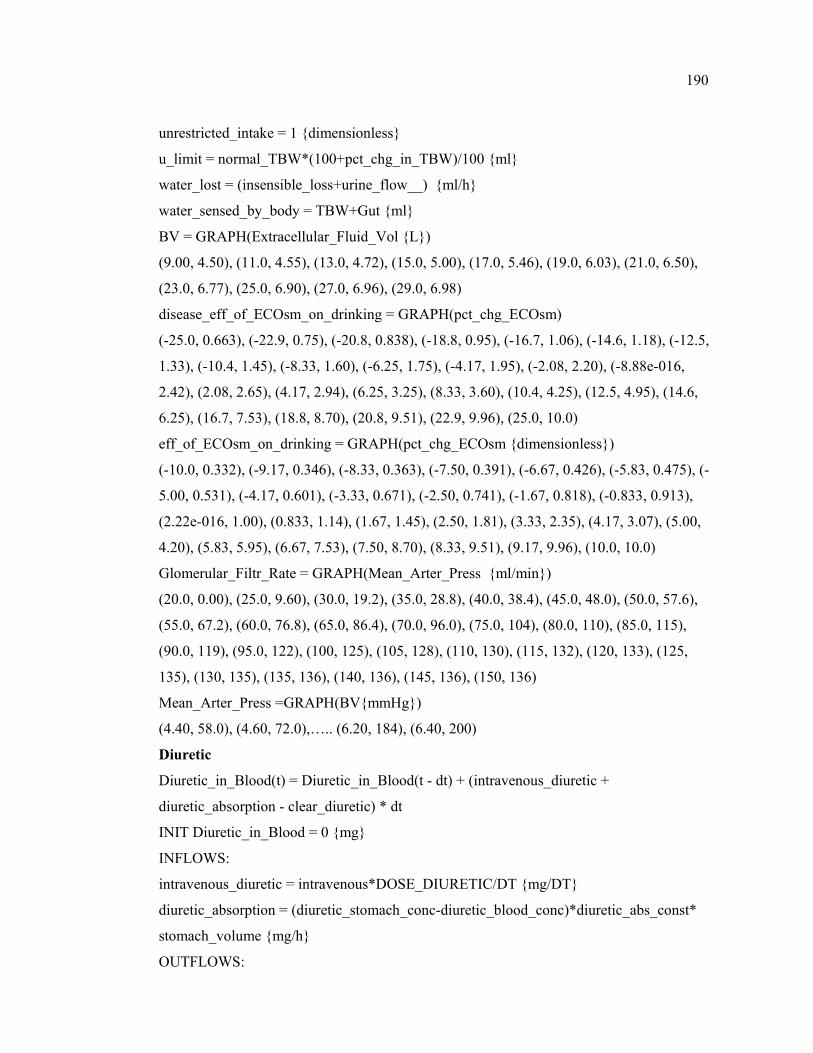
190
unrestricted_intake = 1 {dimensionless}
u_limit = normal_TBW*(100+pct_chg_in_TBW)/100 {ml}
water_lost = (insensible_loss+urine_flow__) {ml/h}
water_sensed_by_body = TBW+Gut {ml}
BV = GRAPH(Extracellular_Fluid_Vol {L})
(9.00, 4.50), (11.0, 4.55), (13.0, 4.72), (15.0, 5.00), (17.0, 5.46), (19.0, 6.03), (21.0, 6.50),
(23.0, 6.77), (25.0, 6.90), (27.0, 6.96), (29.0, 6.98)
disease_eff_of_ECOsm_on_drinking = GRAPH(pct_chg_ECOsm)
(-25.0, 0.663), (-22.9, 0.75), (-20.8, 0.838), (-18.8, 0.95), (-16.7, 1.06), (-14.6, 1.18), (-12.5,
1.33), (-10.4, 1.45), (-8.33, 1.60), (-6.25, 1.75), (-4.17, 1.95), (-2.08, 2.20), (-8.88e-016,
2.42), (2.08, 2.65), (4.17, 2.94), (6.25, 3.25), (8.33, 3.60), (10.4, 4.25), (12.5, 4.95), (14.6,
6.25), (16.7, 7.53), (18.8, 8.70), (20.8, 9.51), (22.9, 9.96), (25.0, 10.0)
eff_of_ECOsm_on_drinking = GRAPH(pct_chg_ECOsm {dimensionless})
(-10.0, 0.332), (-9.17, 0.346), (-8.33, 0.363), (-7.50, 0.391), (-6.67, 0.426), (-5.83, 0.475), (-
5.00, 0.531), (-4.17, 0.601), (-3.33, 0.671), (-2.50, 0.741), (-1.67, 0.818), (-0.833, 0.913),
(2.22e-016, 1.00), (0.833, 1.14), (1.67, 1.45), (2.50, 1.81), (3.33, 2.35), (4.17, 3.07), (5.00,
4.20), (5.83, 5.95), (6.67, 7.53), (7.50, 8.70), (8.33, 9.51), (9.17, 9.96), (10.0, 10.0)
Glomerular_Filtr_Rate = GRAPH(Mean_Arter_Press {ml/min})
(20.0, 0.00), (25.0, 9.60), (30.0, 19.2), (35.0, 28.8), (40.0, 38.4), (45.0, 48.0), (50.0, 57.6),
(55.0, 67.2), (60.0, 76.8), (65.0, 86.4), (70.0, 96.0), (75.0, 104), (80.0, 110), (85.0, 115),
(90.0, 119), (95.0, 122), (100, 125), (105, 128), (110, 130), (115, 132), (120, 133), (125,
135), (130, 135), (135, 136), (140, 136), (145, 136), (150, 136)
Mean_Arter_Press =GRAPH(BV{mmHg})
(4.40, 58.0), (4.60, 72.0),….. (6.20, 184), (6.40, 200)
Diuretic
Diuretic_in_Blood(t) = Diuretic_in_Blood(t - dt) + (intravenous_diuretic +
diuretic_absorption - clear_diuretic) * dt
INIT Diuretic_in_Blood = 0 {mg}
INFLOWS:
intravenous_diuretic = intravenous*DOSE_DIURETIC/DT {mg/DT}
diuretic_absorption = (diuretic_stomach_conc-diuretic_blood_conc)*diuretic_abs_const*
stomach_volume {mg/h}
OUTFLOWS:
191
clear_diuretic = Diuretic_in_Blood/diuretic_clear_del {mg/h}
Diuretic_in_Stomach(t) = Diuretic_in_Stomach(t - dt) + (oral_diuretic -
diuretic_absorption) * dt
INIT Diuretic_in_Stomach = 0 {mg}
INFLOWS:
oral_diuretic = oral*DOSE_DIURETIC/DT {mg/DT}
OUTFLOWS:
diuretic_absorption = (diuretic_stomach_conc-diuretic_blood_conc)*diuretic_abs_const*
stomach_volume {mg/h}
Perceived_Diuretic_conc(t) = Perceived_Diuretic_conc(t-dt) + (correct_diuretic_conc) * dt
INIT Perceived_Diuretic_conc = diuretic_blood_conc {mg}
INFLOWS:
correct_diuretic_conc = (diuretic_blood_conc-Perceived_Diuretic_conc)/diuretic_del
{mg/L/h}
diuretic_abs_const = .693/2 {1/h}
diuretic_blood_conc = Diuretic_in_Blood/BV {mg/L}
diuretic_clear_del = 1.5 {h}
diuretic_del = 0.3 {h}
diuretic_stomach_conc = Diuretic_in_Stomach/stomach_volume {mg/L}
DOSE_DIURETIC = 0 {mg}
Intravenous_Dose_Diuretic = intravenous*DOSE_DIURETIC {mg}
Oral_Dose_Diuretic = oral*DOSE_DIURETIC {mg}
eff_of_diuretic_on_na_excr = GRAPH(Perceived_Diuretic_conc {dimensionless})
(0.00, 1.00), (2.50, 1.08), (5.00, 1.40), (7.50, 1.80), (10.0, 2.33), (12.5, 3.05), (15.0, 3.95),
(17.5, 4.90), (20.0, 5.60), (22.5, 5.90), (25.0, 6.00)
eff_of_diuretic_on_UNa = GRAPH(Perceived_Diuretic_conc {dimensionless})
(0.00, 1.00), (2.50, 0.856), (5.00, 0.687), (7.50, 0.534), (10.0, 0.433), (12.5, 0.374), (15.0,
0.34), (17.5, 0.323), (20.0, 0.315), (22.5, 0.31), (25.0, 0.306)
Initial Values for the Game
Init_ADH = 18000
Init_ADH_Pool = 425992.06
Init_ALD = 2931.22
Init_ANH = 213.17
192
Init_ECNa = 1834.44
Init_Gut = 42.75
Init_Renin = 8274.71
Init_TBW = 44985.59
na_intake_times = 1
set_ADH_conc = 8
Renin-ANG-ALD
ALD(t) = ALD(t - dt) + (ALD_adjust) * dt
INIT ALD = Init_ALD
INFLOWS:
ALD_adjust = (desired_ALD-ALD)/ALD_adj_time {ng/h}
ALD_conc_perceived(t) = ALD_conc_perceived(t - dt) + (ALD_correct) * dt
INIT ALD_conc_perceived = ALD_conc {ng/dl}
INFLOWS:
ALD_correct = (ALD_conc-ALD_conc_perceived)/ALD_conc_perceive_del {ng/h}
Renin(t) = Renin(t - dt) + (renin_secr) * dt
INIT Renin = Init_Renin
INFLOWS:
renin_secr = (desired_renin-Renin)/renin_del
ALD_adj_time = 0.5 {h}
ALD_conc = 100*ALD/normal_TBW {ng/dl}
ALD_conc_normal = 8.5
ALD_conc_perceive_del = 0.5
ALD_ratio_to_normal = ALD_conc/ALD_conc_normal {dimensionless}
ANG_conc = 19.95262315*Renin_ratio
desired_ALD = desired_ALD_conc*normal_TBW/100 {ng}
desired_ALD_conc =
ALD_conc_normal*eff_of_ANG_on_ALD*eff_of_ECNa_conc_on_ALD {ng/dl}
desired_renin = desired_renin_activity*normal_ECFV*1000
desired_renin_activity = normal_renin_activity*eff_of_MAP_on_renin {dimensionless}
log_ANG = LOG10(ANG_conc)
normal_renin_activity = 1 {ng/L}
perceived_ALD_ratio = ALD_conc_perceived/ALD_conc_normal
193
renin_del = 0.25 {h}
Renin_ratio = Renin/normal_ECFV/1000
eff_of_ANG_on_ALD = GRAPH(log_ANG {dimensionless})
(0.00, 0.055), (0.1, 0.11), (0.2, 0.17), (0.3, 0.23), (0.4, 0.29), (0.5, 0.355), (0.6, 0.425), (0.7,
0.49), (0.8, 0.555), (0.9, 0.62), (1, 0.685), (1.10, 0.754), (1.20, 0.85), (1.30, 1.00), (1.40,
1.17), (1.50, 1.67), (1.60, 2.23), (1.70, 2.90), (1.80, 3.75), (1.90, 4.61), (2.00, 5.46), (2.10,
6.51), (2.20, 7.65), (2.30, 8.79)
eff_of_ECNa_conc_on_ALD = GRAPH(ExtracellularNa_conc)
(95.0, 5.28), (98.8, 3.98), (103, 2.98), (106, 2.27), (110, 1.79), (114, 1.49), (118, 1.28), (121,
1.16), (125, 1.08), (129, 1.04), (133, 1.02), (136, 1.01), (140, 1.00)
eff_of_MAP_on_renin = GRAPH(Mean_Arter_Press)
(80.0, 7.58), (83.3, 6.08), (86.7, 4.64), (90.0, 3.38), (93.3, 2.37), (96.7, 1.60), (100.0, 1.00),
(103, 0.72), (107, 0.43), (110, 0.265), (113, 0.17), (117, 0.125), (120, 0.09)
Saline Inf.
Sodium_Load_Given(t) = Sodium_Load_Given(t - dt) + (na_in) * dt
INIT Sodium_Load_Given = 0 {mEq}
INFLOWS:
na_in = na_infused {mEq/h}
Water_Load_given(t) = Water_Load_given(t - dt) + (water_in) * dt
INIT Water_Load_given = 0 {ml}
INFLOWS:
water_in = water_infused/1000 {ml/h}
HYPERTONIC_3%_SALINE = 0 {ml/h}
HYPOTONIC_SALINE = 0 {ml/h}
ISOTONIC_SALINE = 0 {ml/h}
na_infused =
(ISOTONIC_SALINE*0.142+HYPOTONIC_SALINE*0.06+HYPERTONIC_3%_SALIN
E*0.3)/decision_period{mEq/h}
water_infused =
(ISOTONIC_SALINE+HYPERTONIC_3%_SALINE+HYPOTONIC_SALINE)/decision_
period {ml/h}
Sodium (Na)
Extracellular_Na(t) = Extracellular_Na(t - dt) + (na_intake + na_infusion –
194
na_out_in_urine) * dt
INIT Extracellular_Na = Init_ECNa {mEq}
INFLOWS:
na_intake = normal_na_intake*na_intake_times {mEq/h}
na_infusion = na_infused {mEq/h}
OUTFLOWS:
na_out_in_urine = na_out*60 {mEq/h}
ECOsm = ExtracellularNa_conc*2.1
ExtracellularNa_conc = Extracellular_Na/Extracellular_Fluid_Vol {mEq/L}
Filtered_Na = Glomerular_Filtr_Rate*ExtracellularNa_conc/1000
IK = 3550{3500}
IK_conc = IK/Intracellular_Fluid_Vol {mEq/L-for verification}
log_ALD_ratio = LOG10(perceived_ALD_ratio) {dimensionless}
na_excr_ratio = na_out_in_urine/normal_na_excr {dimensionless}
na_intake_plus_infusion = na_intake+na_infusion
na_out =
Filtered_Na*normal_fract*eff_of_ANH_on_na_excr*eff_of_diuretic_on_na_excr*
eff_of_ALD_on_na_excr {mEq/min}
normal_fract = 1/142 {dimensionless}
normal_na_excr = 0.125*60 {mEq/hr}
normal_na_intake = 0.125*60 {mEq/h}
pct_chg_ECOsm = (ECOsm-set_point_ECOsm)/set_point_ECOsm*100 {dimensionless}
set_point_ECOsm = 298.2 {mEq/ml}
eff_of_ALD_on_na_excr = GRAPH(log_ALD_ratio {dimensionless})(-1.00, 2.97), (-0.833,
2.84), (-0.667, 2.56), (-0.5, 2.23), (-0.333, 1.79), (-0.167, 1.37), (-1.67e-016, 1.00), (0.167,
0.765), (0.333, 0.54), (0.5, 0.33), (0.667, 0.195), (0.833, 0.09), (1, 0.045)
eff_of_ANH_on_na_excr = GRAPH(ANH_ratio_to_normal {dimensionless})
(0.00, 0.36), (0.0833, 0.363), (0.167, 0.366), (0.25, 0.37), (0.333, 0.38), (0.417, 0.4), (0.5,
0.43), (0.583, 0.477), (0.667, 0.575), (0.75, 0.71), (0.833, 0.88), (0.917, 0.97), (1.00, 1.00),
(1.08, 1.025), (1.17, 1.05)…. (9.67, 3.60), (9.75, 3.625), (9.83, 3.65), (9.92, 3.675), (10.0,
3.7)
Urinary Na Conc.
escape = IF(ADH_ratio_to_normal>1)THEN(potential_escape)ELSE(1)
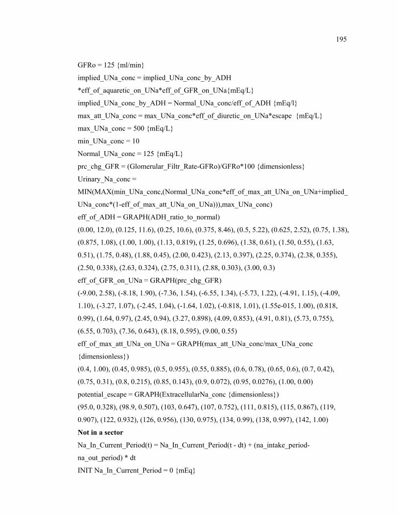
195
GFRo = 125 {ml/min}
implied_UNa_conc = implied_UNa_conc_by_ADH
*eff_of_aquaretic_on_UNa*eff_of_GFR_on_UNa{mEq/L}
implied_UNa_conc_by_ADH = Normal_UNa_conc/eff_of_ADH {mEq/l}
max_att_UNa_conc = max_UNa_conc*eff_of_diuretic_on_UNa*escape {mEq/L}
max_UNa_conc = 500 {mEq/L}
min_UNa_conc = 10
Normal_UNa_conc = 125 {mEq/L}
prc_chg_GFR = (Glomerular_Filtr_Rate-GFRo)/GFRo*100 {dimensionless}
Urinary_Na_conc =
MIN(MAX(min_UNa_conc,(Normal_UNa_conc*eff_of_max_att_UNa_on_UNa+implied_
UNa_conc*(1-eff_of_max_att_UNa_on_UNa))),max_UNa_conc)
eff_of_ADH = GRAPH(ADH_ratio_to_normal)
(0.00, 12.0), (0.125, 11.6), (0.25, 10.6), (0.375, 8.46), (0.5, 5.22), (0.625, 2.52), (0.75, 1.38),
(0.875, 1.08), (1.00, 1.00), (1.13, 0.819), (1.25, 0.696), (1.38, 0.61), (1.50, 0.55), (1.63,
0.51), (1.75, 0.48), (1.88, 0.45), (2.00, 0.423), (2.13, 0.397), (2.25, 0.374), (2.38, 0.355),
(2.50, 0.338), (2.63, 0.324), (2.75, 0.311), (2.88, 0.303), (3.00, 0.3)
eff_of_GFR_on_UNa = GRAPH(prc_chg_GFR)
(-9.00, 2.58), (-8.18, 1.90), (-7.36, 1.54), (-6.55, 1.34), (-5.73, 1.22), (-4.91, 1.15), (-4.09,
1.10), (-3.27, 1.07), (-2.45, 1.04), (-1.64, 1.02), (-0.818, 1.01), (1.55e-015, 1.00), (0.818,
0.99), (1.64, 0.97), (2.45, 0.94), (3.27, 0.898), (4.09, 0.853), (4.91, 0.81), (5.73, 0.755),
(6.55, 0.703), (7.36, 0.643), (8.18, 0.595), (9.00, 0.55)
eff_of_max_att_UNa_on_UNa = GRAPH(max_att_UNa_conc/max_UNa_conc
{dimensionless})
(0.4, 1.00), (0.45, 0.985), (0.5, 0.955), (0.55, 0.885), (0.6, 0.78), (0.65, 0.6), (0.7, 0.42),
(0.75, 0.31), (0.8, 0.215), (0.85, 0.143), (0.9, 0.072), (0.95, 0.0276), (1.00, 0.00)
potential_escape = GRAPH(ExtracellularNa_conc {dimensionless})
(95.0, 0.328), (98.9, 0.507), (103, 0.647), (107, 0.752), (111, 0.815), (115, 0.867), (119,
0.907), (122, 0.932), (126, 0.956), (130, 0.975), (134, 0.99), (138, 0.997), (142, 1.00)
Not in a sector
Na_In_Current_Period(t) = Na_In_Current_Period(t - dt) + (na_intake_period-
na_out_period) * dt
INIT Na_In_Current_Period = 0 {mEq}
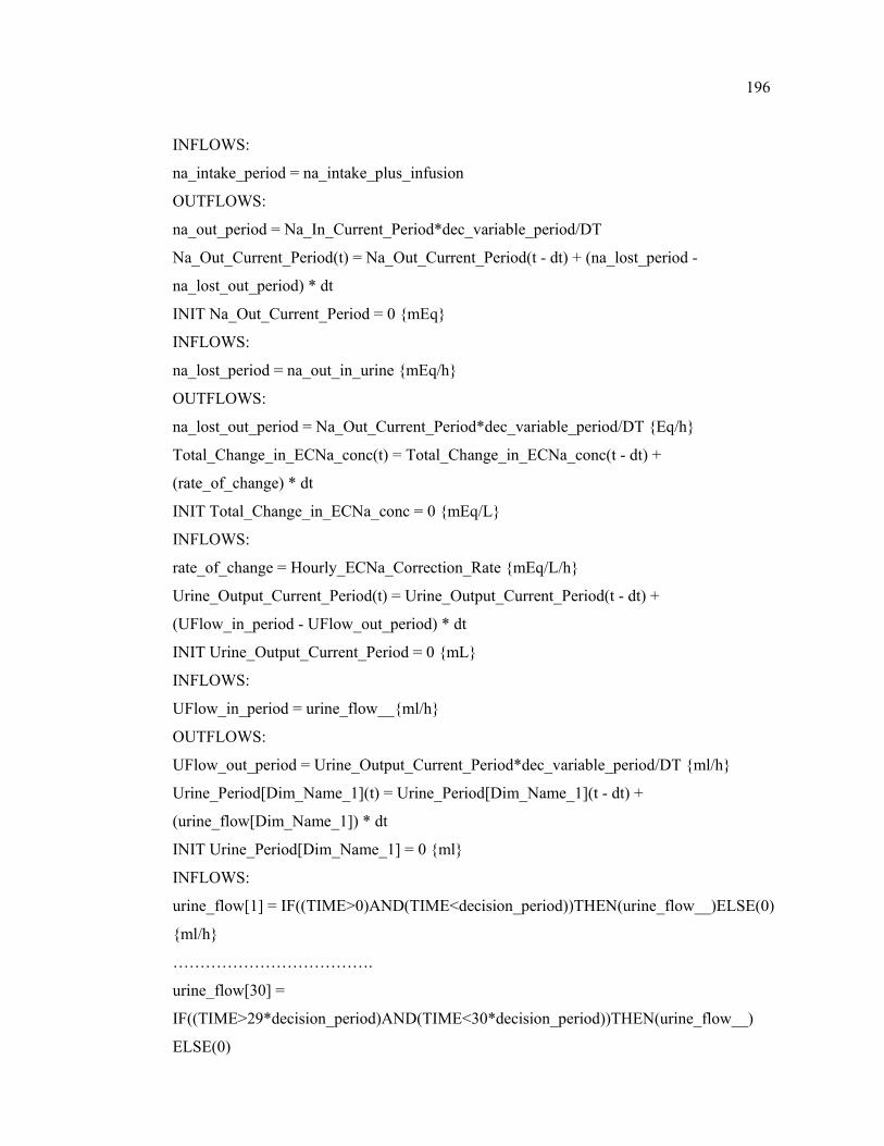
196
INFLOWS:
na_intake_period = na_intake_plus_infusion
OUTFLOWS:
na_out_period = Na_In_Current_Period*dec_variable_period/DT
Na_Out_Current_Period(t) = Na_Out_Current_Period(t - dt) + (na_lost_period -
na_lost_out_period) * dt
INIT Na_Out_Current_Period = 0 {mEq}
INFLOWS:
na_lost_period = na_out_in_urine {mEq/h}
OUTFLOWS:
na_lost_out_period = Na_Out_Current_Period*dec_variable_period/DT {Eq/h}
Total_Change_in_ECNa_conc(t) = Total_Change_in_ECNa_conc(t - dt) +
(rate_of_change) * dt
INIT Total_Change_in_ECNa_conc = 0 {mEq/L}
INFLOWS:
rate_of_change = Hourly_ECNa_Correction_Rate {mEq/L/h}
Urine_Output_Current_Period(t) = Urine_Output_Current_Period(t - dt) +
(UFlow_in_period - UFlow_out_period) * dt
INIT Urine_Output_Current_Period = 0 {mL}
INFLOWS:
UFlow_in_period = urine_flow__{ml/h}
OUTFLOWS:
UFlow_out_period = Urine_Output_Current_Period*dec_variable_period/DT {ml/h}
Urine_Period[Dim_Name_1](t) = Urine_Period[Dim_Name_1](t - dt) +
(urine_flow[Dim_Name_1]) * dt
INIT Urine_Period[Dim_Name_1] = 0 {ml}
INFLOWS:
urine_flow[1] = IF((TIME>0)AND(TIME<decision_period))THEN(urine_flow__)ELSE(0)
{ml/h}
……………………………….
urine_flow[30] =
IF((TIME>29*decision_period)AND(TIME<30*decision_period))THEN(urine_flow__)
ELSE(0)
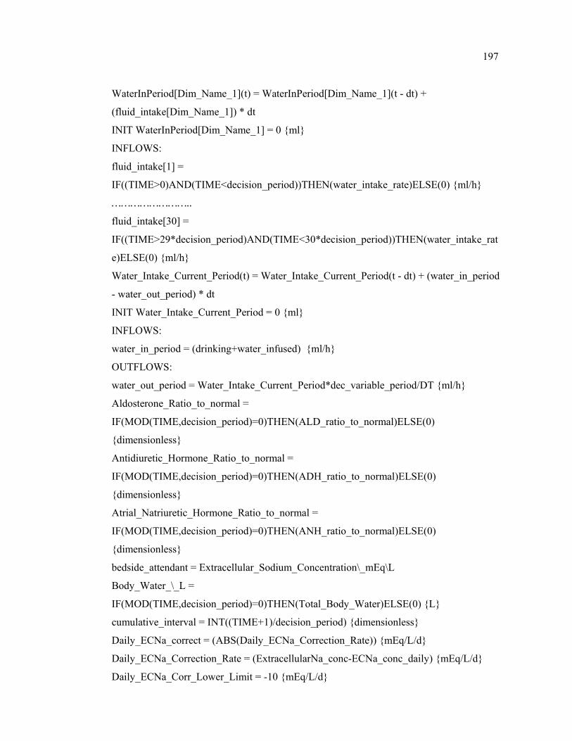
197
WaterInPeriod[Dim_Name_1](t) = WaterInPeriod[Dim_Name_1](t - dt) +
(fluid_intake[Dim_Name_1]) * dt
INIT WaterInPeriod[Dim_Name_1] = 0 {ml}
INFLOWS:
fluid_intake[1] =
IF((TIME>0)AND(TIME<decision_period))THEN(water_intake_rate)ELSE(0) {ml/h}
……………………..
fluid_intake[30] =
IF((TIME>29*decision_period)AND(TIME<30*decision_period))THEN(water_intake_rat
e)ELSE(0) {ml/h}
Water_Intake_Current_Period(t) = Water_Intake_Current_Period(t - dt) + (water_in_period
- water_out_period) * dt
INIT Water_Intake_Current_Period = 0 {ml}
INFLOWS:
water_in_period = (drinking+water_infused) {ml/h}
OUTFLOWS:
water_out_period = Water_Intake_Current_Period*dec_variable_period/DT {ml/h}
Aldosterone_Ratio_to_normal =
IF(MOD(TIME,decision_period)=0)THEN(ALD_ratio_to_normal)ELSE(0)
{dimensionless}
Antidiuretic_Hormone_Ratio_to_normal =
IF(MOD(TIME,decision_period)=0)THEN(ADH_ratio_to_normal)ELSE(0)
{dimensionless}
Atrial_Natriuretic_Hormone_Ratio_to_normal =
IF(MOD(TIME,decision_period)=0)THEN(ANH_ratio_to_normal)ELSE(0)
{dimensionless}
bedside_attendant = Extracellular_Sodium_Concentration\_mEq\L
Body_Water_\_L =
IF(MOD(TIME,decision_period)=0)THEN(Total_Body_Water)ELSE(0) {L}
cumulative_interval = INT((TIME+1)/decision_period) {dimensionless}
Daily_ECNa_correct = (ABS(Daily_ECNa_Correction_Rate)) {mEq/L/d}
Daily_ECNa_Correction_Rate = (ExtracellularNa_conc-ECNa_conc_daily) {mEq/L/d}
Daily_ECNa_Corr_Lower_Limit = -10 {mEq/L/d}
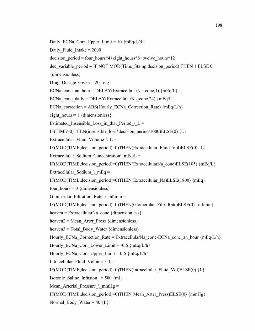
198
Daily_ECNa_Corr_Upper_Limit = 10 {mEq/L/d}
Daily_Fluid_Intake = 2000
decision_period = four_hours*4+eight_hours*8+twelve_hours*12
dec_variable_period = IF NOT MOD(Time_Stamp,decision_period) THEN 1 ELSE 0
{dimensionless}
Drug_Dosage_Given = 20 {mg}
ECNa_conc_an_hour = DELAY(ExtracellularNa_conc,1) {mEq/L}
ECNa_conc_daily = DELAY(ExtracellularNa_conc,24) {mEq/L}
ECNa_correction = ABS(Hourly_ECNa_Correction_Rate) {mEq/L/h}
eight_hours = 1 {dimensionless}
Estimated_Insensible_Loss_in_that_Period_\_L =
IF(TIME>0)THEN(insensible_loss*decision_period/1000)ELSE(0) {L}
Extracellular_Fluid_Volume_\_L =
IF(MOD(TIME,decision_period)=0)THEN(Extracellular_Fluid_Vol)ELSE(0) {L}
Extracellular_Sodium_Concentration\_mEq\L =
IF(MOD(TIME,decision_period)=0)THEN(ExtracellularNa_conc)ELSE(105) {mEq/L}
Extracellular_Sodium_\_mEq =
IF(MOD(TIME,decision_period)=0)THEN(Extracellular_Na)ELSE(1800) {mEq}
four_hours = 0 {dimensionless}
Glomerular_Filtration_Rate_\_ml\min =
IF(MOD(TIME,decision_period)=0)THEN(Glomerular_Filtr_Rate)ELSE(0) {ml/min}
heaven = ExtracellularNa_conc {dimensionless}
heaven2 = Mean_Arter_Press {dimensionless}
heaven3 = Total_Body_Water {dimensionless}
Hourly_ECNa_Correction_Rate = ExtracellularNa_conc-ECNa_conc_an_hour {mEq/L/h}
Hourly_ECNa_Corr_Lower_Limit = -0.6 {mEq/L/h}
Hourly_ECNa_Corr_Upper_Limit = 0.6 {mEq/L/h}
Intracellular_Fluid_Volume_\_L =
IF(MOD(TIME,decision_period)=0)THEN(Intracellular_Fluid_Vol)ELSE(0) {L}
Isotonic_Saline_Infusion_ = 500 {ml}
Mean_Arterial_Pressure_\_mmHg =
IF(MOD(TIME,decision_period)=0)THEN(Mean_Arter_Press)ELSE(0) {mmHg}
Normal_Body_Water = 40 {L}
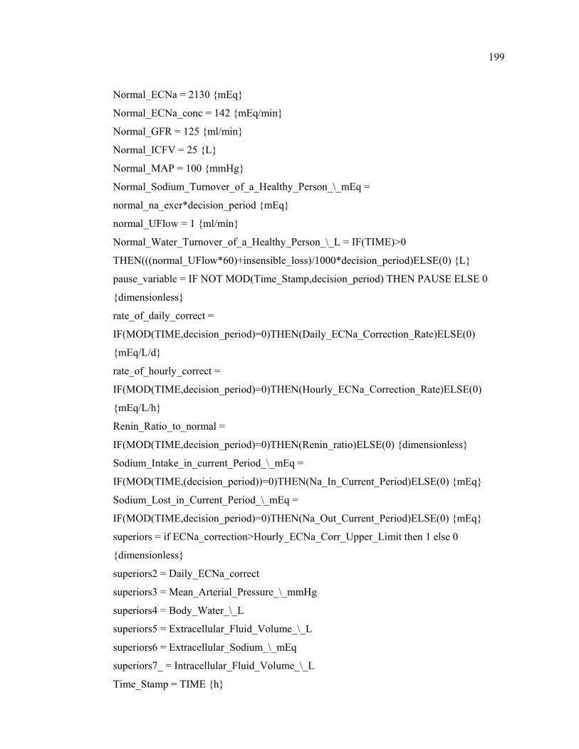
199
Normal_ECNa = 2130 {mEq}
Normal_ECNa_conc = 142 {mEq/min}
Normal_GFR = 125 {ml/min}
Normal_ICFV = 25 {L}
Normal_MAP = 100 {mmHg}
Normal_Sodium_Turnover_of_a_Healthy_Person_\_mEq =
normal_na_excr*decision_period {mEq}
normal_UFlow = 1 {ml/min}
Normal_Water_Turnover_of_a_Healthy_Person_\_L = IF(TIME)>0
THEN(((normal_UFlow*60)+insensible_loss)/1000*decision_period)ELSE(0) {L}
pause_variable = IF NOT MOD(Time_Stamp,decision_period) THEN PAUSE ELSE 0
{dimensionless}
rate_of_daily_correct =
IF(MOD(TIME,decision_period)=0)THEN(Daily_ECNa_Correction_Rate)ELSE(0)
{mEq/L/d}
rate_of_hourly_correct =
IF(MOD(TIME,decision_period)=0)THEN(Hourly_ECNa_Correction_Rate)ELSE(0)
{mEq/L/h}
Renin_Ratio_to_normal =
IF(MOD(TIME,decision_period)=0)THEN(Renin_ratio)ELSE(0) {dimensionless}
Sodium_Intake_in_current_Period_\_mEq =
IF(MOD(TIME,(decision_period))=0)THEN(Na_In_Current_Period)ELSE(0) {mEq}
Sodium_Lost_in_Current_Period_\_mEq =
IF(MOD(TIME,decision_period)=0)THEN(Na_Out_Current_Period)ELSE(0) {mEq}
superiors = if ECNa_correction>Hourly_ECNa_Corr_Upper_Limit then 1 else 0
{dimensionless}
superiors2 = Daily_ECNa_correct
superiors3 = Mean_Arterial_Pressure_\_mmHg
superiors4 = Body_Water_\_L
superiors5 = Extracellular_Fluid_Volume_\_L
superiors6 = Extracellular_Sodium_\_mEq
superiors7_ = Intracellular_Fluid_Volume_\_L
Time_Stamp = TIME {h}
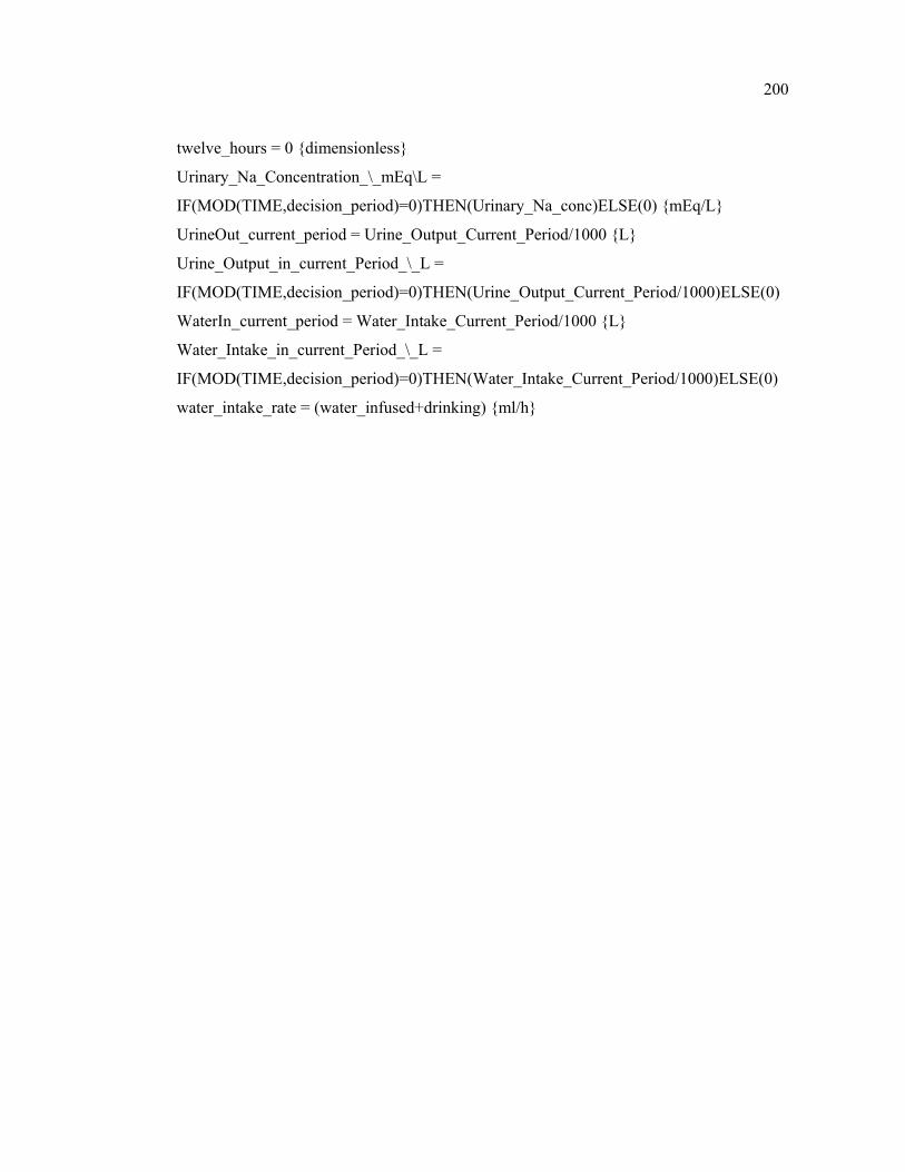
200
twelve_hours = 0 {dimensionless}
Urinary_Na_Concentration_\_mEq\L =
IF(MOD(TIME,decision_period)=0)THEN(Urinary_Na_conc)ELSE(0) {mEq/L}
UrineOut_current_period = Urine_Output_Current_Period/1000 {L}
Urine_Output_in_current_Period_\_L =
IF(MOD(TIME,decision_period)=0)THEN(Urine_Output_Current_Period/1000)ELSE(0)
WaterIn_current_period = Water_Intake_Current_Period/1000 {L}
Water_Intake_in_current_Period_\_L =
IF(MOD(TIME,decision_period)=0)THEN(Water_Intake_Current_Period/1000)ELSE(0)
water_intake_rate = (water_infused+drinking) {ml/h}
201
APPENDIX D: GLOSSARY
Aldosterone: Aldosterone is a mineralocorticoid, adrenocortical hormone that possesses a
high sodium-retaining ability.
Angiotensin: Angiotensin is the most powerful vasoconstrictor agent made by the body,
and also the most potent direct stimulus for the release of aldosterone by the zona
glomerulosa of the adrenal cortex.
Atrial Natriuretic Hormone (ANH): A hormone that is secreted from the atrial tissue of
the heart. ANH causes an increase in electrolyte excretion rates and urine volume.
Antidiuretic Hormone (ADH): A hormone that is secreted by the pituitary gland. ADH is
involved in controlling body water and osmolality.
Aquaretic (ADH-Antagonist): A category of drugs that are used in the management of
patients with water excess and consequent dilutional hyponatremia.
Diabetes Insipidus/Polyuria: The passage of more than 2 liters of dilute fluid through the
body. This condition may be due to the failure of ADH release (hypothalamic DI) or failure
of the kidney to respond to ADH (nephrogenic DI).
Diuretic: A category of drugs that are used in the management of body fluid disorders such
as edema or hyponatremia.
Diuresis: An increased rate of urine, which can be of two types: water diuresis and solute or
osmotic diuresis
202
Euvolemia: Normal blood volume.
Extracellular Sodium Concentration: Amount of sodium contained in one liter of
extracellular fluid, usually expressed as mmol or mEq/L.
Glomerular Filtration Rate (GFR): The GFR is the amount of filtrate formed per minute
in all nephrons of both kidneys. In the adult male, this rate is about 125 ml/min; in the
female about 110 ml/min.
Hypervolemia: Elevated blood volume.
Hypovolemia: Reduced blood volume.
Molality: The number of moles of a solute per kilogram of solvent
Molarity: The number of moles of solute per liter of solution
Natriuresis: Natriuresis /osmotic diuresis results when more solute is presented to the
kidney than they reabsorb. In contrast to water diuresis, urine flow rate depends upon
urinary solute content.
Osmolality: The number of osmoles per liter of water (solvent). The osmole is 1 g
molecular weight of a nonionizable solute.
Osmolarity: The number of osmoles per liter of solution.
Osmosis: Osmosis is the net diffusion of water across a selectively permeable membrane
from a region of high water concentration to one that has a lower water concentration.
203
Polyuria: See Diabetes Insipidus.
Renin-Angiotensin-Aldosterone System (RAAS): The Renin-Angiotensin-Aldosterone
system is one of the most powerful regulators of sodium and potassium balance and arterial
blood pressure. These three functions are regulated by changes in Angiotensin and
Aldosterone levels in response to wide variations in dietary intake of sodium and potassium.
Renin: Renin is a specific enzyme produced in the kidney, which is stimulated by decreases
in blood volume and/or pressure.
Tonicity: The effective osmolality which is equal to the sum of the concentrations of the
solutes which have the capacity to exert an osmotic force across the membrane. Tonicity is
a term used frequently in a medical context.
Urinary sodium concentration: Amount of sodium contained in one liter of urine, usually
expressed as mmol or mEq/L.
Water diuresis: The production of a large volume of a dilute urine which results when
water ingested or administered is in excess of body requirements.
204
REFERENCES
Abbrecht, P.H., 1980, “Regulation of Extracellular Fluid Volume and Osmolality”, Annals
of Biomedical Engineering, Vol: 8, pp. 461-472.
Bagby, S.P. and W. M. Bennett, 1998, “Differentiating Disorders of ECF Volume/ Na
Content Regulation versus Disorders of Total Body Fluid Osmolarity/ Water
Regulation”, Advances in Physiology Education, Vol. 20, No: 1, pp. 169-184.
Bankir, L., 2001, “Antidiuretic Action of Vasopressin: Quantitative Aspects and Interaction
between V1a and V2 Receptor-Mediated Effects”, Cardiovascular Research, Vol. 51,
pp. 372-390.
Barlas, Y., 1996, “Formal Aspects of Model Validity and Validation in System Dynamics”,
System Dynamics Review, Vol.12, No.3, pp. 183-210.
Bray, J.J, P.A. Cragg, and A.D.C. Macknight, 1989, Lecture Notes on Human Physiology,
Oxford, Boston: Blackwell Scientific Publications; Chicago, Ill.: Distributor, USA,
Year Book Medical Publishers, c1989.
Brandis, K., 2005, “Fluid Physiology - an on-line text"
http://www.anaesthesiamcq.com/FluidBook/index.php.
Bricker, N.S., 1967, “The Control of Sodium Excretion with Normal and Reduced Nephron
Populations. The Pre-eminence of Third Factor”, The American Journal of Medicine,
Vol: 43, pp. 313-321.
205
Cameron, W. H., 1977, “A Model Framework for Computer Simulation of Overall Renal
Function”, Journal of Theoretical Biology, Vol: 66, pp. 551-572.
Cannon, W, 1939, The Wisdom of the Body, N.Y. Norton.
Carson, E.R., C. Cobelli and L. Finkelstein, 1983, The Mathematical Modeling of
Metabolic and Endocrine Systems, New York: Wiley.
Cogan, E., M.F. Debieve, T. Pepersack, M. Abramov, 1988, “Natriuresis and Atrial
Natriuretic Factor Secretion during Inappropriate Antidiuresis”, The American
Journal of Medicine, Vol. 84, pp. 409-418.
Coleman, T.G. and J. E. Hall, 1992, “A Mathematical Model of Renal Hemodynamics and
Excretory Function”, in Structuring Biological Systems- A Computer Modeling
Approach, edited by S. Sitharama Iyengar, CRC Press.
Cumming, A and W. Plant, 2003, “Water, Electrolyte and Acid-Base Imbalance”, In:
Davidson’s Principles & Practice of Medicine, Elsevier Health Sciences.
Decaux, G., 2001, “Long-term Treatment of Patients with Inappropriate Secretion of
Antidiuretic Hormone by the Vasopressin Receptor Antagonist Conivaptan, Urea, or
Furosemide”, The American Journal of Medicine, Vol: 110, No: 7, pp. 582-584.
DeHaven J.C., Shapiro N.Z., 1967, “On the control of urine formation”, Nephron, Vol: 4,
Suppl 4, pp. 1-63.
Deshmukh S., C. Thomas, 2005, “Syndrome of Inappropriate Secretion of Antidiuretic
Hormone”, http://www.emedicine.com/med/topic3541.htm
206
Ecelbarger, C.A., C. Chou, A. J. Lee, S. R. DiGiovanni, J.G. Verbalis and M. A. Knepper,
1998, “Escape from Vasopressin-Induced Antidiuresis: Role of Vasopressin
Resistance of the Collecting Duct”, American Journal of Physiology, Vol: 274 (6 Pt
2), pp. 1161-1166.
Edoute, Y., M. R. Davids, C. Johnston and M.L. Halperin, 2003, “An Integrative
Physiological Approach to Polyuria and Hyponatremia: a ‘double-take’ on the
Diagnosis and Therapy in a Patient with Schizophrenia”, Q.J. Med, Vol: 96, pp. 531-
540.
Goh, K.P., 2004, “Management of Hyponatremia”, American Family Physician, Vol: 69,
pp. 2387-2394.
Guyton, A.C., T.G. Coleman, 1967, “Long Term Regulation of the Circulation:
Interrelationships with Body Fluid Volumes”. In: Physical Bases of Circulatory
Transport: Regulation and Exchange, edited by E.B. Reeve, and A.C. Guyton.
Philadelphia: W.B. Saunders Company.
Guyton, A. C., T. G. Coleman, and H. J. Granger, 1972, “Circulation: Overall Regulation”,
Annu. Rev. Physiol.Vol: 34, pp. 13-46.
Guyton, A. C., T.G. Coleman, D.B. Young, T.E.Lohmeier, and J. W. DeClue, 1980, “Salt
Balance and Long-Term Blood Pressure Control”, Ann. Rev. Med., Vol: 31, pp. 15-
27.
Guyton, A.C., J.E. Hall., 2000, Textbook of Medical Physiology. Philadelphia: W.B.
Saunders Company.
207
Halperin M.L., 2002, “Body Compartment Volumes and Composition After Giving a
Vasopressin Antagonist”, Nephrol Dial Transplant, Vol: 17, No: 2, pp. 300-303.
Halperin, M.L and D. Bohn, 2002, “Clinical Approach to Disorders of Salt and Water
Balance; Emphasis on Integrative Physiology”, Critical Care Clinics, Vol: 18, No: 2,
pp. 249-272.
Haslett, C., Chilvers, Boon, E. R., Colledge, N.A., N.R., J.A. Hunter, (eds.), 2003,
Davidson’s Principles and Practice of Medicine, Elsevier Health Sciences.
Hirshberg, B, A. Ben-Yehuda, 1997, “The Syndrome of Inappropriate Antidiuretic
Hormone Secretion in the Elderly”, American Journal of Medicine, Vol: 103, pp. 270-
273.
Ikeda, N., F. Marumo, M. Shirataka and T. Sato, 1979, “A Model of Overall Regulation of
Body Fluids”, Annals of Biomedical Engineering, Vol: 7, pp. 135-166.
Ishikawa, S., T. Saito, K. Kasono, 2004, “Pathological Role of Aquaporin-2 in Impaired
Water Excretion and Hyponatremia”, Journal of Neuroendocrinology, Vol: 16, pp.
293-296.
Jamison, R. L and R.E. Oliver, 1982, “Disorders of Urinary Concentration and Dilution”,
The American Journal of Medicine, Vol: 72, pp. 308-322.
Janicic N. and J.G. Verbalis, 2003, “Evaluation and Management of Hypo-osmolality in
Hospitalized Patients”, Endocrinology and Metabolism Clinics of North America,
Vol: 32, pp.459-481.
208
Janssen, W.M.T., 1994, Atrial Natriuretic Factor- Integrated Effects on Blood Pressure,
Natriuresis, and Renal Medullary Blood Flow in Man, Ph. D. Thesis, Rijksuniversiteit
Groningen.
Karaaslan, F., 2004, Modeling and Analysis of the Interaction Between Renal Symphathetic
Nerve Activity, Arterial Pressure and Sodium Excretion, PhD Thesis, Bogazici
University.
Kasper, D.L., E. Braunwald, A. Fauci, S. Hauser, D. Longo, J.L. Jameson, 2004, Harrison’s
Principles of Internal Medicine, McGraw-Hill.
Kaye, M., 1966, “An Investigation into the Cause of Hyponatremia in the Syndrome of
Inappropriate Secretion of Antidiuretic Hormone”, The American Journal of
Medicine, Vol: 41, No: 6, pp. 910-926.
Laragh J.H., 1985, “Atrial Natriuretic Hormone the renin-aldosterone axis, and blood
pressure-electrolyte homeostasis”, New England Journal of Medicine, Vol: 313, No:
21, pp. 1330-1340.
Navar, L., 1997, “The Kidney in Blood Pressure Regulation and Development of
Hypertension”, Medical Clinics of North America, Vol: 81, No: 5, pp. 1165-1198.
Northrop, R.B., 2000, “Hormonal Regulation of Sodium, Potassium, Calcium and
Magnesium Ions”, in: Endogeneous and Exogeneous Regulation and Control of
Physiological Systems, Boca Raton, Fla.: Chapman & Hall/CRC, c2000.
Palm, C., D. Reimann and P. Gross, 2001, “The Role of V2 Vasopressin Antagonists in
Hyponatremia”, Cardiovascular Research, Vol. 51, pp. 403–408.
209
Reeve, E.B. and L. Kulhanek, 1967, “Regulation of Body Water Content: A Preliminary
Analysis”, in: Physical Bases of Circulatory Transport: Regulation and Exchange,
edited by E.B. Reeve, and A.C. Guyton. Philadelphia: W.B. Saunders Company.
Sagawa, Kiichi, 1975, “Critique of a Large-scale Organ System Model: the Guytonian
Cardiovascular Model”, Annals of Biomedical Engineering, Vol: 3, No: 4, pp. 386-
400.
Saito, T., S. Ishikawa, K. Abe, K. Kamoi, K. Y1amada, K. Shimizu, T. Saruta and S.
Yoshida, 1996, “Acute Aquaresis by the Nonpeptide Arginine Vasopressin(AVP)
Antagonist OPC-31260 Improves Hyponatremia in Patients with Syndrome of
Endocrinology and Metabolism, Vol. 82, No: 4, pp. 1054-1057.
Schwartz, W.B., W. Bennett, S. Curelop, F.C. Bartter, 2001, “A Syndrome of Renal Sodium
Loss and Hyponatremia Probably Resulting from Inappropriate Secretion of
Antidiretic Hormone”, Journal of the American Society of Nephrology, Vol: 12,
pp.2860-2870, reprinted from The American Journal of Medicine Vol: 23 pp. 529-
542, 1957.
Shafiee, M.A.S., D. Bohn, E. J. Hoorn and M. L. Halperin, 2003, “How to Select Optimal
Maintenance Intravenous Fluid Therapy”, Q. J. Med, Vol. 96, pp. 601-610.
Schrier, R.W. and M. Niederberger, 1993, “Paradoxes of Body Fluid Volume Regulation in
Health and Disease: a Unifying Hypothesis”, West J Med, Vol. 164, pp. 393–408.
Smith, P., 1998, “Body Fluid Compartments”,
http://www.liv.ac.uk/~petesmif/teaching/1bds_mb/notes/fluid/text.htm
210
Song, J., X. Hu, O. Khan, Y. Tian, J.G. Verbalis and C. Ecelbarger, 2004, “Increased Blood
Pressure, Aldosterone Activity, and Regional Differences in Renal ENaC protein
During Vasopressin Escape”, American Journal of Physiology Renal Physiology, Vol.
287, No: 5, pp. 1076-1083.
Sonnenblick, M., Y. Friedlander, A.J. Rosin, 1993, “Diuretic Induced Severe
Hyponatremia-Review and Analysis of 129 Reported Patients”, Chest, Vol: 103, No:
2, pp. 601-606.
Sterman, J.D., 2000, Business Dynamics: Systems Thinking and Modeling in a Complex
World. McGraw-Hill, Boston.
Sterns, R.H, 1987, “Severe Symptomatic Hyponatremia: Treatment and Outcome. A Study
of 64 Cases”, Annals of Internal Medicine, Vol: 107, pp. 656-664.
Strand, F.L., 1983, Physiology- A Regulatory Systems Approach, New York: Macmillan.
Toates, F.M. and K. Oatley, 1970, “Computer Simulation of Thirst and Water Balance”,
Medical and Biological Engineering, Vol: 8, pp.71-87.
Toates, F.M. and K. Qatley, 1977, “Control of Water Excretion by Antidiuretic Hormone:
Some Aspects of Modelling the System”, Medical and Biological Engineering and
Computing, Vol: 15, No: 6, pp.579-588.
Uttamsingh, R. J., M.S. Leaning, J.A. Bushman, E.R. Carson and L. Finkelstein, 1985,
“Mathematical Model of the Human Renal System”, Medical and Biological
Engineering and Computing, Vol: 23, pp. 525-536.
211
Verbalis, J.G., M.D. Drutarosky, R.J.Ertel, R.R. Vollmer, 1989, “Adaptive Responses to
Sustained Volume Expansion in Hyponatraemic Rats”, The Journal of Endocrinology,
Vol: 122, pp. 421-431.
Verbalis, J.G., 1992, “Pathogenesis of Hyponatremia in an Experimental Model of the
Syndrome of Inappropriate Antidiuresis”, American Journal of Physiology, Vol: 267,
pp. 1617-1625.
Verbalis, J.G., 1998, “Adaptation to Acute and Chronic Hyponatremia: Implications for
Symptomatology, Diagnosis, and Therapy”, Semin. Nephrol, Vol: 18, No: 1, pp. 3-19.
Verbalis, J.G., 1998, “Studies of Renal Aquaporin-2 Expression During Renal Escape from
Vasopressin-induced Antidiuresis”, Advances in Experimental Medicine and Biology,
Vol: 449, pp. 395-406.
Verbalis, J.G., 2003, “Disorders of Body Water Homeostasis”, Best Practice & Research
Clinical Endocrinology & Metabolism, Vol. 17, No. 4, pp. 471–503.
Vieweg, W.V., L.S. Godleski, 1988, “Hyponatremia and Atrial Natriuretic Peptide
Secretion in Patients with Vasopressin-induced Antidiuresis”, American Journal of
Medicine, Vol: 85, pp. 594-595.
Weir, M.R., V.J. Dzau, 1999, “The Renin-Angiotensin-Aldosterone System: a Specific
Target for Hypertension Management”, American Journal of Hypertension, Vol: 12,
pp. 205-213.
Wong, L.L. and J.G. Verbalis, 2001, “Vasopressin V2 Receptor Antagonists”,
Cardiovascular Research, Vol. 51, No: 3, pp. 391-402.
212
Wong, L.L. and J.G. Verbalis, 2002, “Systemic Diseases Associated withDisorders of
Water Homeostasis”, Endocrinology and Metabolism Clinics of North America, Vol:
31, No: 1, pp. 121-140.
Yamamura Y., Ogawa H., Chihara T., Kondo K., Onogawa T., Nakamura S., Mori
T.,Tominaga M. and Yabuuchi Y., 1991, “OPC-21268, an Orally Effective,
Nonpeptide Vasopressin V1 Receptor Antagonist”, Science, Vol. 252, pp. 572–574.
Yamamura Y., Ogawa H., Yamashita H., Chihara T., Miyamoto H., Nakamura S., Onogawa
T., Yamashita T., Hosokawa T., Mori T., Tominaga M. and Yabuuchi Y., 1992,
“Characterization of a Novel Aquaretic Agent, OPC-31260, as an Orally Effective,
Nonpeptide Vasopressin V2 Receptor Antagonist”, Br J Pharmacol Vol. 105, pp.
787–791.
Yamamura, Y., A.Ohnishi, R.Okahara, H. Fujihara, T. Inoue, y. Yabuuchi, T. Tanaka, 1993,
“Potent Aquaretic Agent. A Novel Nonpeptide Selective Vasopressin 2 Antagonist
(OPC-31260) in Men”, J. Clin. Invest, Vol: 92, pp. 2653-2659.
Yamasaki, Y., T. Nishiuchi, A. Kojima, H. Saito, 1988, “Effects of an Oral Water Load and
Intravenous Administration of Isotonic Glucose, Hypertonic Saline, Mannitol and
Furosemide on the Release of Atrial Natriuretic Peptide in Men”, Acta
Endocrinologica, Vol: 119, pp. 269-276.
Zerbe, R. and G. Robertson, 1980, “Vasopressin Function in the Syndrome of Inappropriate
Antidiuresis”, Annual Review of Medicine, Vol: 31, pp. 315-327.
213
REFERENCES NOT CITED
Abraham W.T. and R.W. Schrier, 1994, “Body Fluid Volume Regulation in Health and
Disease”, Advances in Internal Medicine, Vol: 39, pp. 23-47.
Akay, M. and A. Marsh (ed.s), 2001, Information Technologies in Medicine, Volume 1,
Medical Simulation and Education, Wiley- IEEE Computer Society PR.
Al-Salman, J., D. Kemp and D. Randall, 2002, “Hyponatremia”, The Western Journal of
Medicine, Vol: 176, pp. 173-176.
Baylis, 2003, “The Syndrome of Inappropriate Antidiuretic Hormone Secretion”, The
International Journal of Biochemistry & Cell Biolog, Vol: 35, No: 11, pp. 1495-1499.
Beuter, A., L. Glass, M.C. Mackey, M.S. Titcombe (ed.s), 2003, Nonlinear Dynamics in
Physiology and Medicine (Interdisciplinary Applied Mathematics, V.25). Springer
Verlag.
Bigelow, J.H, J.C. DeHaven and M.L. Shapley, 1973, “Systems Analysis of the Renal
Function”, Journal of Theoretical Biology, Vol: 41, pp. 287-322.
Bookallil, R., 2002, “Sodium Abnormalities in the Neurosurgical Patient”, Current
Anaesthesia & Critical Care, Vol: 13, No: 3, pp. 153-158.
Brown, J.H.U. and D. S. Gann, (ed.s), 1973, Engineering Principles in Physiology,
Academic Press, New York and London.
214
Carson, E. and C. Cobelli, 2000, Modeling Methodology for Physiology and Medicine
(Academic Press Biomedical Engineering Series), Academic Press.
Davids, M. R., Y. Edoute, J.P. Mallie, D. G. Bichet and M.L. Halperin, 2002, “Body
Compartment Volumes and Composition after Giving a Vasopressin Antagonist:
Changes are Revealed by a Tonicity Balance”, Nephrol Dial Transplant, Vol: 17, pp.
300-303.
Decaux, G., 2001, “Difference in Solute Excretion during Correction of Hyponatremic
Patients with Cirrhosis or Syndrome of Inappropriate Secretion of Antidiuretic
Hormone by Oral Vasopressin V2 Receptor Antagonist VPA-985”, J Lab Clin Med.,
Vol. 138, No: 1, pp.18-21.
Flood, R. L, 1985, Quantitative Modelling of the Fluid-Electrolyte, Acid-Base Balance for
Clinical Application, Ph. D. Thesis , The City University, Department of Systems
Science.
Ford, A., 1999, Modeling the Environment: An Introduction to System Dynamics Modeling
of Environmental Systems, Island Press, Washington.
Granger, J.P., 1998, “Regulation of Extracellular Fluid Volume by Integrated Control of
Sodium Excretion”, Advances in Physiology Education, Vol: 275, pp. 157-168.
Gross, P., D. Reimann, J. Neidel, C. Doke, F. Prospert, G. Decaux, J. Verbalis, R.W.
Schrier, 1998, “The Treatment of Severe Hyponatremia”, Kidney International
Supplement, Vol: 64, pp. 6-11.
Guyton, A.C., 1991, “Blood Pressure Control-Special Role of the Kidneys and Body
Fluids”, Science, Vol: 252, pp. 1813-1816.
215
Hall, J.E, Guyton, A.C., and M.W. Brands, 1996, “Pressure-Volume Regulation in
Hypertension”, Kidney International, Vol: 49, Suppl. 55, pp. 35-41
Hargrove, J.L., 1998, Dynamic Modeling in the Health Sciences (Modeling Dynamic
Systems), Springer Verlag.
Kawai, N., A. Baba, T. Suzuki and H. Shiraishi, 2001, “Roles of Arginine Vasopressin and
Atrial Natriuretic Peptide in Polydipsia-Hyponatremia of Schizophrenic Patients”,
Psychiatry Research, Vol. 101, pp. 39-45.
Keener, J., J. Sneyd, 1998, Mathematical Physiology, Springer-Verlag.
Khoo, M.C.K., Physiological Control Systems: Analysis, Simulation, and Estimation,
Wiley-IEEE Press.
Kimura, T., K. Abe, K. Omata, M. Shoji, K. Kudo, K. Matsui, M. Inoue, M. Yasujima, K.
Yoshinaga, 1986, “Effects of Acute Water Load, Hypertonic Saline Infusion, and
Furosemide Administration on Atrial Natriuretic Peptide and Vasopressin Release in
Humans”, The Journal of Clinical Endocrinology and Metabolism, Vol: 62, pp. 1003-
1010.
Khoo, M.C.K., 1999, Physiological Control Systems: Analysis, Simulation, and Estimation.
Wiley-IEEE Computer Society Pr.,
Kofranek, J., L.D.Vu, H. Snaselova, R. Kerekes, T. Velan, 2001, “GOLEM—multimedia
simulator for medical education”, Medinfo, Vol. 10, No: 2, pp. 1042-1046.
Lawrence J. Goldstein and E. B. Rypins, 1992, “A Computer Model of the Kidney”,
Computer Methods and Programs in Biomedicine, Vol: 37, No: 3, pp. 191-203.
216
Leaning M.S., R.L. Flood, D.G. Cramp, E.R. Carson, 1985, “A System of Models for Fluid-
Electrolyte Dynamics”, IEEE Trans Biomed Eng., Vol: 32, No: 10, pp. 856-864.
Minhtri K. Nguyen, Ira Kurtz, 2003, “A New Quantitative Approach to the Treatment of
Dysnatremias”, Clin Exp Nephrology, Vol: 7, No: 2, pp.125-137.
Petra c.m. Donati-Genet, 2001, “Acute Symptomatic Hyponatremia and Cerebral Salt
Wasting After”, Journal of Pediatric Surgery, Vol: 36, No: 7, pp. 1094-1097.
Richards, A.M., H. Ikram, T.G. Yandle, M.G. Nicholls, M.W.I. Webster, E.A. Espiner,
1985, “Renal, Haemodynamic, and Hormonal Effects of Human Alpha Atrial
Natriuretic Peptide in Healthy Volunteers”, The Lancet, Vol: 1, pp.545-549.
Rideout, V.C, 1991, Mathematical and Computer Modeling of Physiological Systems,
Englewood Cliffs, N.J.: Prentice Hall.
Riggs, D.S, 1970, Control Theory and Physiological Feedback Mechanisms, Baltimore:
Williams and Wilkins.
Roman, R. J. and F. R. Sias, 1985, “Network Computer Analysis of the Human Kidney”,
Mathematical Modelling, Vol: 7, pp. 1045-1069.
Sagnella, G.A., A. C. Shore, N. D. Markandu, G.A. MacGregor, 1985, “Effects of Changes
in Dietary Sodium Intake and Saline Infusion on Immunoreactive Atrial Natriuretic
Peptide in Human Plasma”, The Lancet, Vol: 2, pp. 1208-1210.
Shindel, A., G. Tobin, C. Klutke, 2002, “Hyponatremia Associated with Desmopressin for
the Treatment of Nocturnal Polyuria”, Urology, Vol: 60, No: 2, pp. 344.
217
Shimizu, K., 1995, “Aquaretic Effects of the Nonpeptide V2 Antagonist OPC-31260 in
Hydropenic Humans”, Kidney International, Vol: 48, pp. 220-226.
Sodeman, W., and T.M. Sodeman, 1985, Sodeman’s Pathologic Physiology, Philadelphia:
W.B. Saunders Co., Washington.
Suzuki, 2002, “Roles of Arginine Vasopressin and Atrial natriuretic peptide in polydipsia-
hyponatremia of schizophrenic patients”, Pschiatry Research, Vol: 101, No: 1, pp.39-
45.
Yamamura Y., S. Nakamura, S. Itoh, T. Hirano, T. Onogawa, T. Yamashita, Y. Yamada, K.
Tsujimae, M. Aoyama, K. Kotosai, H. Ogawa, H. Yamashita, K. Kondo, M.
Tominaga, G. Tsujimoto and T. Mori, 1998, “OPC-41061, a Highly Potent Human
Vasopressin V2-Receptor Antagonist: Pharmacological Profile and Aquaretic Effect
by Single and Multiple Oral Dosing in Rats”, The Journal of Pharmacology and
Experimental Therapeutics, Vol: 287, pp. 860-867.


![Pandur Dynamic Driving Simulator - Analysis of mine blast ... · Pandur Dynamic Driving Simulator - Analysis of mine blast effects Armando J. Loureiro da Silva ... mass of 6 [Kg]](https://img.pdfslide.net/doc/110x75/5e6d513b241fb16f2e44f9e7/pandur-dynamic-driving-simulator-analysis-of-mine-blast-pandur-dynamic-driving.jpg)