Policy Research Working Paper 7051

A Dynamic Spatial Model of Rural-Urban Transformation with Public Goods

Dan BillerLuis Andres

David Cuberes

South Asia Region

October 2014

WPS7051P

ublic

Dis

clos

ure

Aut

horiz

edP

ublic

Dis

clos

ure

Aut

horiz

edP

ublic

Dis

clos

ure

Aut

horiz

edP

ublic

Dis

clos

ure

Aut

horiz

edP

ublic

Dis

clos

ure

Aut

horiz

edP

ublic

Dis

clos

ure

Aut

horiz

edP

ublic

Dis

clos

ure

Aut

horiz

edP

ublic

Dis

clos

ure

Aut

horiz

ed

Produced by the Research Support Team

Abstract

The Policy Research Working Paper Series disseminates the findings of work in progress to encourage the exchange of ideas about development issues. An objective of the series is to get the findings out quickly, even if the presentations are less than fully polished. The papers carry the names of the authors and should be cited accordingly. The findings, interpretations, and conclusions expressed in this paper are entirely those of the authors. They do not necessarily represent the views of the International Bank for Reconstruction and Development/World Bank and its affiliated organizations, or those of the Executive Directors of the World Bank or the governments they represent.

Policy Research Working Paper 7051

This paper is a product of the Sustainable Development Department, South Asia Region. It is part of a larger effort by the World Bank to provide open access to its research and make a contribution to development policy discussions around the world. Policy Research Working Papers are also posted on the Web at http://econ.worldbank.org. The authors may be contacted at dbiller@worldbank.org, landres@worldbank.org, and d.cuberes@sheffield.ac.uk.

This paper develops a dynamic model that explains the pattern of population and production allocation in an economy with an urban location and a rural one. Agglomer-ation economies make urban dwellers benefit from a larger population living in the city and urban firms become more productive when they operate in locations with a larger labor force. However, congestion costs associated with a

too large population size limit the process of urban-rural transformation. Firms in the urban location also ben-efit from a public good that enhances their productivity. The model predicts that in the competitive equilibrium the urban location is inefficiently small because house-holds fail to internalize the agglomeration economies and the positive effect of public goods in urban production.

A Dynamic Spatial Model of Rural-Urban Transformation with Public Goods

Dan Biller, Luis Andres, David Cuberes1

JEL codes: H40, R1, R23

keywords: rural-urban transformation; agglomeration economies; congestion costs; public goods

1 Dan Biller and Luis Andres are respectively Sector Manager and Lead Economist at the World Bank Group. David Cuberes is a Lecturer at the University of Sheffield, UK. Contact author: d.cuberes@sheffield.ac.uk

A Dynamic Spatial Model of Rural-Urban

Transformation with Public Goods

1 Introduction

Urbanization - defined as the percentage of a country’s population that lives

in urban areas- among developing countries exhibits significant variation across

different world regions and countries. The Middle East and North Africa region

is the most urbanized region, with around 70% of its population living in cities.

By contrast, South Asia has a surprisingly low urbanization, around 28%. Dif-

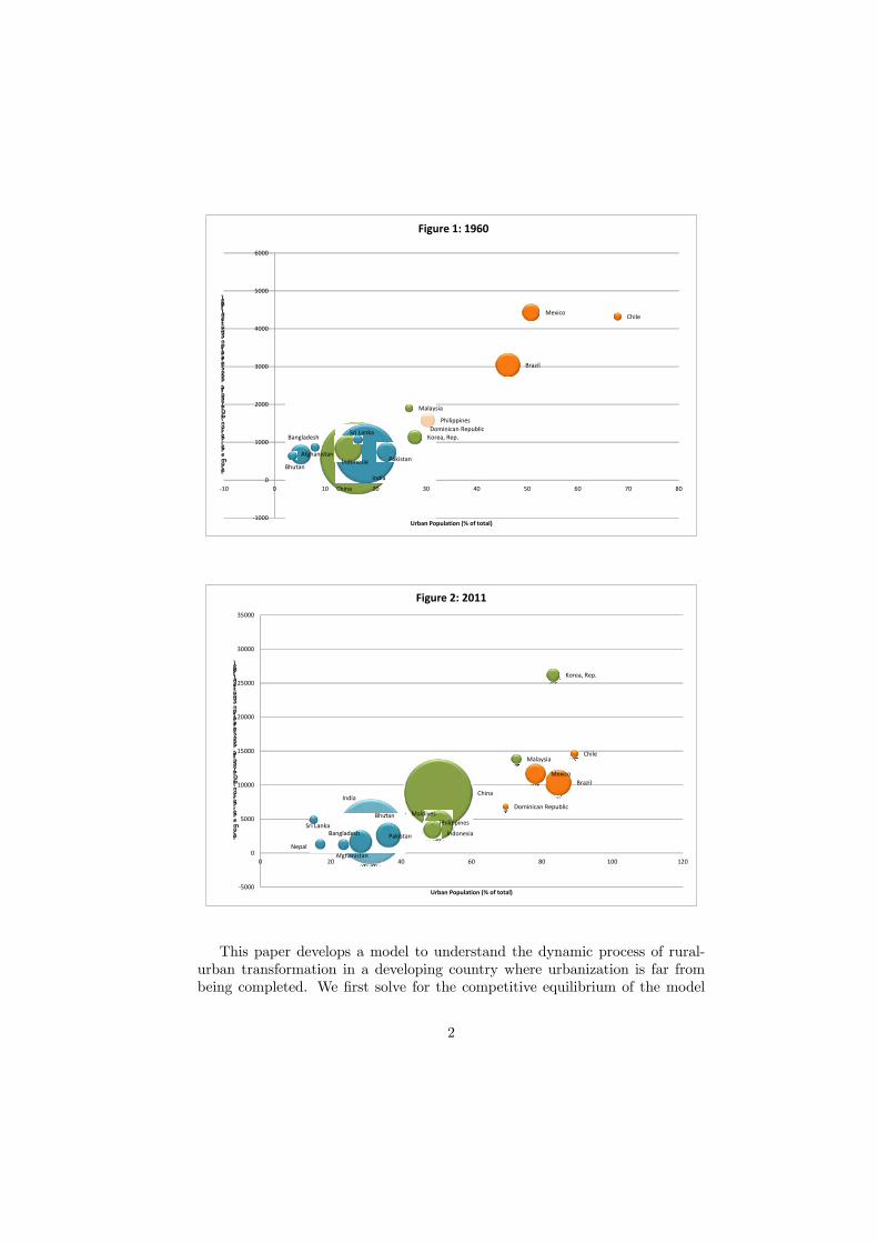
ferences in income per capita cannot account for this variation. Figure 1 shows

the level of urbanization and annual GDP per capita in PPP terms in selected

developing countries around the world in 1960.1 South Asia and East Asia are

clustered together, while Latin American economies are slightly detached given

their higher GDP per capita PPP and larger urbanization levels. In this figure

the size of the bubbles represent countries with their population size — the larger

the bubble the larger the population. Figure 2 shows that in half a century East

Asia followed the Latin American path with some countries like the Republic

of South Korea and Malaysia even surpassing Latin American economies both

on urbanization levels and on GDP per capita PPP, but South Asia lagged well

behind. The eight countries of South Asia (Afghanistan, Bangladesh, Bhutan,

India, The Maldives, Nepal, Pakistan, and Sri Lanka) display very low urban-

ization given their income levels.2

1This figure is similar to the one presented in Henderson (2009) which shows the variation

in urbanization rates at different levels of income for different countries. He emphasizes that

China’s urbanization rate is also too low at its stage of development.2These figures are constructed grouping countries by region according to the World Bank

classification. See http://www.worldbank.org/depweb/beyond/beyondco/beg_ce.pdf

1

Afghanistan

Bangladesh

Brazil

Chile

China

Dominican Republic

India

Indonesia

Korea, Rep.

Malaysia

Mexico

BhutanPakistan

Philippines

Sri Lanka

‐1000

0

1000

2000

3000

4000

5000

6000

‐10 0 10 20 30 40 50 60 70 80

Income Per Person (GDP/capita, PPP $Infalation‐adjusted) (log)

Urban Population (% of total)

Figure 1: 1960

Afghanistan

Bangladesh

Bhutan

Brazil

Chile

China

Dominican Republic

India

Indonesia

Korea, Rep.

Malaysia

Maldives

Mexico

Nepal

Pakistan

PhilippinesSri Lanka

‐5000

0

5000

10000

15000

20000

25000

30000

35000

0 20 40 60 80 100 120

Income Per Person (GDP/capita, PPP $Infalation‐adjusted) (log)

Urban Population (% of total)

Figure 2: 2011

This paper develops a model to understand the dynamic process of rural-

urban transformation in a developing country where urbanization is far from

being completed. We first solve for the competitive equilibrium of the model

2

and then we find the optimal solution of a benevolent social planner. In both

cases we focus on the analysis of the steady-state of the model. The study of

both positive and normative aspects of urbanization make this paper of interest

from an academic point of view but also for policymakers wishing to address

specific problems related to the process of urbanization.3

Probably the best known model of urbanization is the so-called Harris-

Todaro model (Harris and Todaro, 1970). In their paper they develop a simple

static theory in which there are two sectors in the economy, a modern one and

an agricultural one, with declining marginal productivity in both of them. This

implies that the higher the wage is, the lower is the demand for workers in both

sectors. The Harris-Todaro model has clear predictions on labor migration, but

it ignores technological differences between the rural and urban areas as well as

the dynamics of the urbanization process. Chan and Yu (2010), Neary (1981,

1988) and Riadh (1998) have added capital goods to this model and solved for

its dynamics, although their emphasis is again on labor migration between two

technologically identical regions.

Another strand of the literature has sprung as a result of the interest in

the field of urban economics in understanding the process of city formation.

There exist several papers that study urban processes in the presence of capi-

tal goods (Anas, 1978, 1992; Kanemoto, 1980; Henderson and Ioannides, 1981;

Miyao,1981; Fujita, 1982; Ioannides, 1994; Palivos and Wang, 1996). One im-

portant limitation of these models is that they assume free mobility of all factors

of production. A direct consequence of this assumption is that these models pre-

dict large and rapid swings in the population of cities that reach a critical level

and that, when new cities form, their population jumps instantly to some ar-

bitrarily large size. This leads to counterfactual predictions - the existing data

on cities’ population exhibit smooth fluctuations as countries urbanize. By con-

trast, in our model the population of rural and urban areas changes smoothly

over time because of the assumption that investment in capital goods is irre-

versible. To our knowledge, only the papers by Henderson and Venables (2009)

and Cuberes (2009) explicitly assume irreversibility in capital investment, hence

solving the problem of sudden changes in cities’ population. The former present

a model in which cities form in sequential order as a consequence of the presence

of increasing returns in production and congestion costs.

The model by Cuberes (2009) is closely related to the one analyzed here but

our framework has several important differences. First, Cuberes (2009) analyzes

city formation only and does not consider rural areas. Second, agglomeration

benefits only firms, not consumers directly. Third, there are no public goods in

3Some papers have studied the effect of different policies on the process of urbanization.

Henderson and Kuncoro (1996), for example, show the effects of favoritism for certain regions

in Indonesia. Other cases are discussed in Henderson (1988), Lee and Choe (1990), and

Jefferson and Singhe (1999).

3

the analysis. While it is also the case that in his model the competitive equilib-

rium is inefficient, the present model is richer since the inefficiency comes both

from preferences and production and because it discusses normative implica-

tions of the model. The main goal of Cuberes (2009) is to rationalize a pattern

of sequential growth between existing cities, whereas the model in the present

paper introduces sufficient structure to explain the process of migration from a

rural location to an urban one.

The new economic geography models presented in Fujita et al (2001) are

also related to our analysis. In their benchmark core-periphery model there are

sectors, a manufacturing one, where production takes place under monopolistic

competition, and an agricultural one, where goods are produced under perfect

competition. Their model also includes transporting goods across the regions in

the form of iceberg costs so that a fraction proportional to the distance between

the locations is lost in the trading process. In these models, urbanization is the

result of technological progress or productivity differentials across regions. Our

model significantly simplifies the analysis by assuming a single homogeneous

good - as opposed to an agricultural good and a manufactured one - and no

transport costs. These two simplifications allow us to introduce a capital good

in the model which, in turn, generates more realistic dynamics than the ones in

standard economic geography models. A second advantage of our model is that

we explicitly model the fact that private agents do not internalize the benefits

associated with agglomeration economies.

In terms of policy implications, the literature is more scarce. As stated in

Fujita et al. (2001) this is probably due to the fact that there is a need for better

empirical studies to pin down the exact external economies and diseconomies

associated with urban agglomerations. Along these lines, Au and Henderson

(2006) estimate a theoretical model of city formation using Chinese data and

conclude that most cities in China are undersized. However, their model does

not study the process of urbanization per se and they do not analyze market

failures and the related policy implications. The main aim of their paper is

to empirically estimate the inverse U-shape pattern predicted by theirs and

many other models in the literature (Henderson, 1974; Helsley and Strange,

1990; Black and Henderson, 1999; Fujita at al., 2001; Duranton and Puga,

2001) by using measures of urban economies but also urban diseconomies.4 The

theoretical model of Henderson and Wang (2005) studies the process of rural-

urban spatial transformation as a country urbanizes. The model is based on

a system of cities and it focuses on explaining how the number of cities and

their size evolves in a context of positive population growth. Our model does

not have population growth and consequently it does not consider city creation.

However, these simplifications allow us to compare the decentralized and efficient

equilibrium in more detail. Finally, Henderson and Wang (2007) analyze, from

an empirical point of view, how urbanization is accommodated by increases in

4Rosenthal and Strange (2004) and Moretti (2004) offer reviews of these papers.

4

numbers and sizes of cities.5

The rest of the paper is organized as follows. Section 2 presents the decen-

tralized model and solves its steady-state equilibrium. Section 3 does the same

for the problem of a benevolent social planner. Section 4 presets a numerical

example that allows us to compare the predictions of the two problems. Finally,

Section 4 concludes the paper.

2 A Spatial Equilibrium Model of Rural-Urban

Transformation

2.1 Setup

Our model is based on Cuberes (2009). The economy is closed and populated by

a large number of agents who work and live in one of two possible locations:

an urban one () and a rural one ().

2.2 The Decentralized Problem

2.2.1 Households

The maximization problem of a representative agent is contingent to the location

where she lives.6

Location U There are agents living in location at period . Utility

in location is given by ( ,Φ( )), where

≡

denotes consumption

of the private good in per capita terms in location . The function Φ() is

increasing and it reflects the existence of an originated from network effects,

knowledge spillovers, information sharing, companionship, safety, among others.

The function is increasing and concave in the two inputs.

An agent in location has two sources of income: her wage earnings and

the returns to her investment in the only asset in the economy, namely physical

capital in location . Let’s denote the investment in asset . The agent ’s

budget constraint is then:

= + −

where is the wage rate in and is the return on the private asset .

7

The intertemporal problem of a representative agent is given by:

5Richardson (1987) presents a cost-benefit analysis of the urbanization process in four

different countries and proposes some policies to adress different policy issues.6For simplicity, the model assumes that households live and work in the same location.7We assume that the investment in the physical good must be positive. This assumption

is clarified in the firm’s problem. In the agent’s optimization problem we further assume that

this non-negativity constraint on investment is not binding, that is household invest a positive

amount in every period.

5

max

Z ∞0

− ( Φ( ))

= + −

0 given

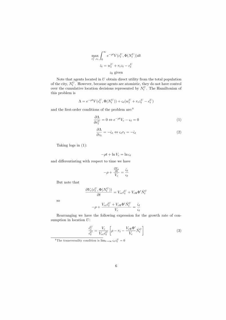
Note that agents located in obtain direct utility from the total population

of the city, . However, because agents are atomistic, they do not have control

over the cumulative location decisions represented by . The Hamiltonian of

this problem is

Λ = − ( Φ( )) + (

+

− )

and the first-order conditions of the problem are:8

Λ

= 0⇔ − − = 0 (1)

Λ

= − ⇔ = − (2)

Taking logs in (1):

−+ ln = ln and differentiating with respect to time we have

−+

=

But note that

( Φ(

))

=

+ ΦΦ

0

so

−+ + ΦΦ

0

=

Rearranging we have the following expression for the growth rate of con-

sumption in location :

=

∙− − ΦΦ

0

¸(3)

8The transversality condition is lim→∞ = 0

6

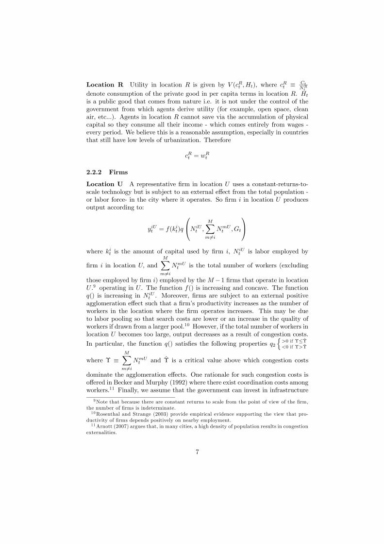
Location R Utility in location is given by ( ), where ≡

denote consumption of the private good in per capita terms in location .

is a public good that comes from nature i.e. it is not under the control of the

government from which agents derive utility (for example, open space, clean

air, etc...). Agents in location cannot save via the accumulation of physical

capital so they consume all their income - which comes entirely from wages -

every period. We believe this is a reasonable assumption, especially in countries

that still have low levels of urbanization. Therefore

=

2.2.2 Firms

Location U A representative firm in location uses a constant-returns-to-

scale technology but is subject to an external effect from the total population -

or labor force- in the city where it operates. So firm in location produces

output according to:

= ()

⎛⎝

X6=

⎞⎠where is the amount of capital used by firm ,

is labor employed by

firm in location and

X6=

is the total number of workers (excluding

those employed by firm ) employed by the −1 firms that operate in location .9 operating in . The function () is increasing and concave. The function

() is increasing in . Moreover, firms are subject to an external positive

agglomeration effect such that a firm’s productivity increases as the number of

workers in the location where the firm operates increases. This may be due

to labor pooling so that search costs are lower or an increase in the quality of

workers if drawn from a larger pool.10 However, if the total number of workers in

location becomes too large, output decreases as a result of congestion costs.

In particular, the function () satisfies the following properties 2

n0 if Υ≤Υ0 if ΥΥ

where Υ ≡X6=

and Υ is a critical value above which congestion costs

dominate the agglomeration effects. One rationale for such congestion costs is

offered in Becker and Murphy (1992) where there exist coordination costs among

workers.11 Finally, we assume that the government can invest in infrastructure

9Note that because there are constant returns to scale from the point of view of the firm,

the number of firms is indeterminate.10Rosenthal and Strange (2003) provide empirical evidence supporting the view that pro-

ductivity of firms depends positively on nearby employment.11Arnott (2007) argues that, in many cities, a high density of population results in congestion

externalities.

7

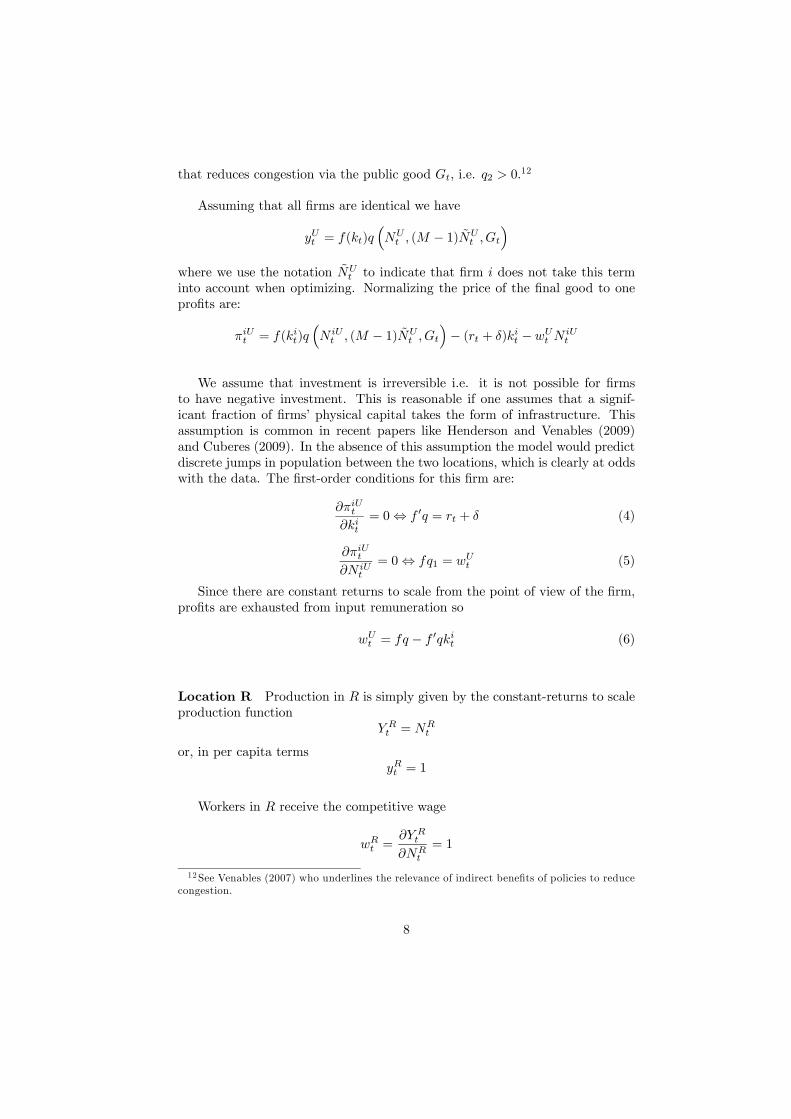
that reduces congestion via the public good , i.e. 2 0.12

Assuming that all firms are identical we have

= ()³ ( − 1)

´where we use the notation

to indicate that firm does not take this term

into account when optimizing. Normalizing the price of the final good to one

profits are:

= ()³ ( − 1)

´− ( + ) −

We assume that investment is irreversible i.e. it is not possible for firms

to have negative investment. This is reasonable if one assumes that a signif-

icant fraction of firms’ physical capital takes the form of infrastructure. This

assumption is common in recent papers like Henderson and Venables (2009)

and Cuberes (2009). In the absence of this assumption the model would predict

discrete jumps in population between the two locations, which is clearly at odds

with the data. The first-order conditions for this firm are:

= 0⇔ 0 = + (4)

= 0⇔ 1 = (5)

Since there are constant returns to scale from the point of view of the firm,

profits are exhausted from input remuneration so

= − 0 (6)

Location R Production in is simply given by the constant-returns to scale

production function

=

or, in per capita terms

= 1

Workers in receive the competitive wage

=

= 1

12 See Venables (2007) who underlines the relevance of indirect benefits of policies to reduce

congestion.

8

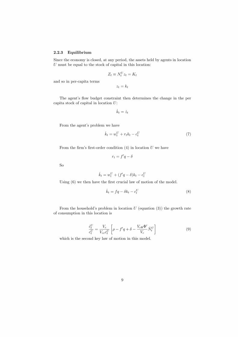
2.2.3 Equilibrium

Since the economy is closed, at any period, the assets held by agents in location

must be equal to the stock of capital in this location:

≡ =

and so in per-capita terms

=

The agent’s flow budget constraint then determines the change in the per

capita stock of capital in location :

=

From the agent’s problem we have

= + − (7)

From the firm’s first-order condition (4) in location we have

= 0 −

So

= + (

0 − ) −

Using (6) we then have the first crucial law of motion of the model.

= − − (8)

From the household’s problem in location (equation (3)) the growth rate

of consumption in this location is

=

∙− 0 + − ΦΦ

0

¸(9)

which is the second key law of motion in this model.

9

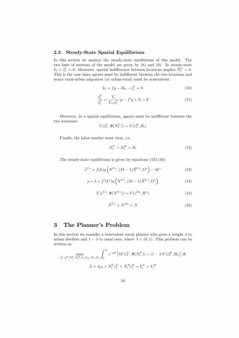
2.3 Steady-State Spatial Equilibrium

In this section we analyze the steady-state equilibrium of this model. The

two laws of motions of the model are given by (8) and (9). In steady-state

= = 0. Moreover, spatial indifference between locations implies = 0.

This is the case since agents must be indifferent between the two locations and

hence rural-urban migration (or urban-rural) must be nonexistent.

= − − = 0 (10)

=

[− 0 + ] = 0 (11)

Moreover, in a spatial equilibrium, agents must be indifferent between the

two locations:

( Φ( )) = ( )

Finally, the labor market must clear, i.e.

+

= (12)

The steady-state equilibrium is given by equations (13)-(16):

∗ = ()³∗ ( − 1)∗ ∗

´− ∗ (13)

+ = 0(∗)³∗ ( − 1)∗∗

´(14)

(∗Φ(∗)) = (∗∗) (15)

∗ +∗ = (16)

3 The Planner’s Problem

In this section we consider a benevolent social planner who gives a weight to

urban dwellers and 1− to rural ones, where ∈ (0 1). This problem can be

written as

max

Z ∞0

−£ ( Φ(

)) + (1− ) ( )

¤

+ +

+

=

+

10

= ()

¡

¢ =

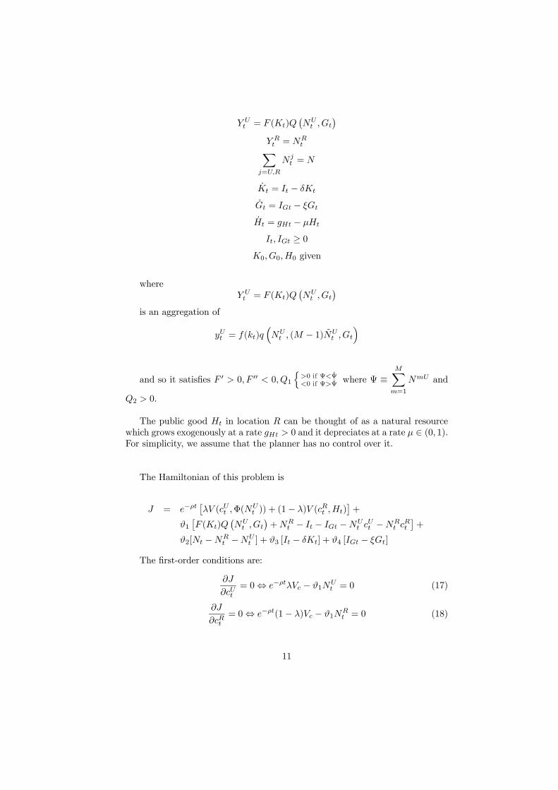
X=

=

= −

= −

= −

≥ 00 00 given

where

= ()

¡

¢is an aggregation of

= ()³ ( − 1)

´

and so it satisfies 0 0 00 01

n0 if ΨΨ

0 if ΨΨwhere Ψ ≡

X=1

and

2 0.

The public good in location can be thought of as a natural resource

which grows exogenously at a rate 0 and it depreciates at a rate ∈ (0 1).For simplicity, we assume that the planner has no control over it.

The Hamiltonian of this problem is

= −£ ( Φ(

)) + (1− ) ( )

¤+

1£ ()

¡

¢+

− − −

−

¤+

2[ − −

] + 3 [ − ] + 4 [ − ]

The first-order conditions are:

= 0⇔ − − 1

= 0 (17)

= 0⇔ −(1− ) − 1

= 0 (18)

11

= 0⇔ −ΦΦ0 + 1[ ()

¡

¢− ]− 2 = 0 (19)

= 0⇔ 1[1− ]− 2 = 0 (20)

≤ 0⇔ −1 + 3 ≤ 0 (21)

≤ 0⇔ −1 + 4 ≤ 0 (22)

= −3 ⇔ 10()

¡

¢− 3 = −3 (23)

= −4 ⇔ 1 ()

¡

¢− 4 = −4 (24)

Assuming the inequalities are binding we have

3 = 1 = 4

so

3 = 1 = 4

and then we have from (3)

1

1= − 0()

¡

¢(25)

From (17) we have

− = 1

Taking logs and differentiating over time we have

=

"+ − 0()

¡

¢+

µ1− ΦΦ

0

¶#(26)

where we use the fact that

( Φ(

))

=

+ ΦΦ

0

Equation (26) represents the growth rate of consumption per capita in location

in the planner’s problem.

Similarly, taking logs in (18) and differentiating with respect to time we

obtain the growth rate of consumption in location :

12

=

"+ − 0()

¡

¢+

−

#(27)

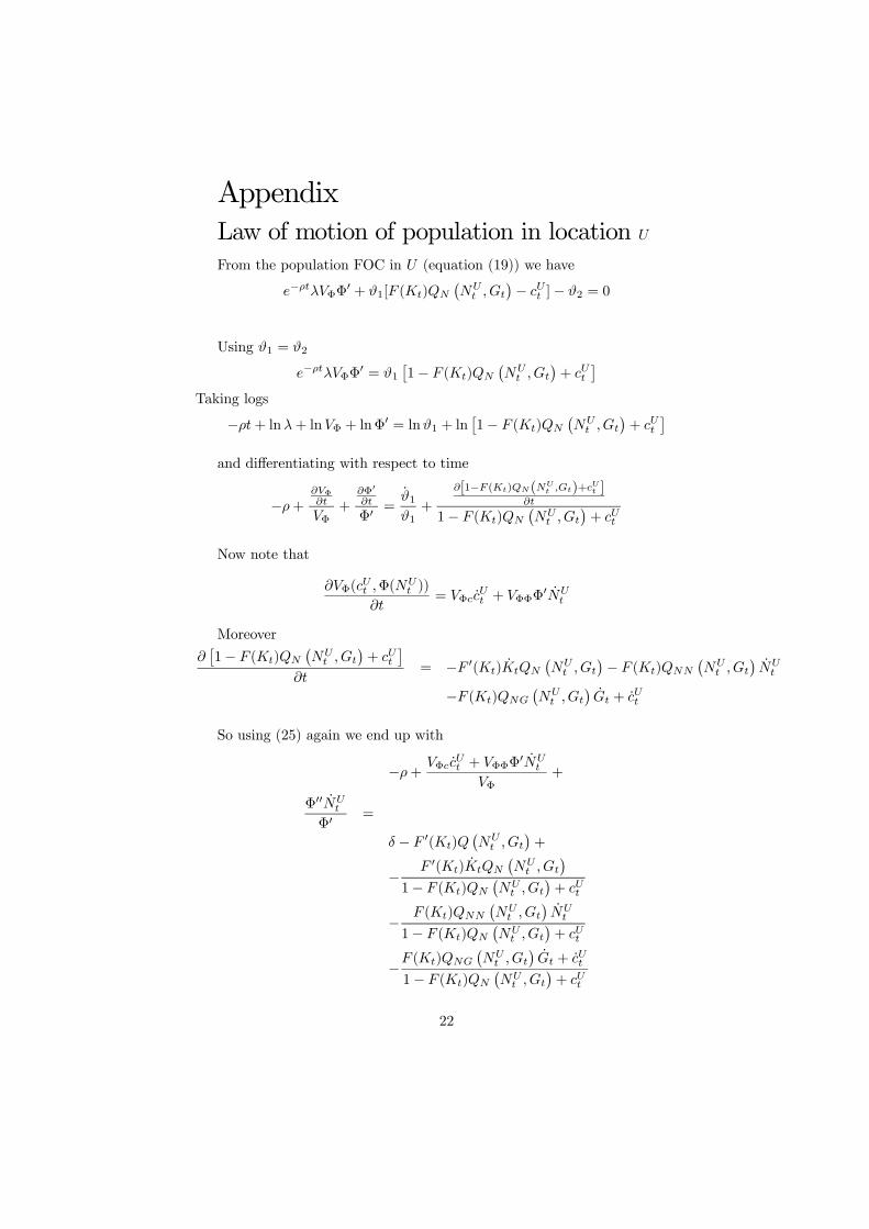
From the population FOC in (equation (19)) we have

−ΦΦ0 + 1[ ()

¡

¢− ]− 2 = 0

Using 1 = 2

−ΦΦ0 = 1£1− ()

¡

¢+

¤In the Appendix we show that taking logs and differentiating with respect to

time gives us the law of motion of population in :

=1

Ω

⎡⎢⎢⎢⎢⎣− Φ

Φ+ − 0()

¡

¢− 0()( )

1− ()( )+

− 1− ()(

)+

− ()( )

1− ()( )+

⎤⎥⎥⎥⎥⎦(28)

where Ω ≡ ΦΦΦ0

Φ+Φ00

Φ0 + ()(

)

1− ()( )+

.

From the FOC with respect to (equation 25) we have

= −4 ⇔ 1 ()

¡

¢− 4 = −4

But since

1 = 4

we have

1 ()

¡

¢− 1 = −1Dividing both sides by 1 and using (25) we get

()

¡

¢− = 0()¡

¢− (29)

This condition states that the planner sets the net marginal benefit of the

public good equal to the net opportunity cost of investment not used in the

capital good. It is important to notice that this condition was not present in

the decentralized equilibrium.

13

3.1 Steady-State Spatial Equilibrium

In this section we analyze the steady-state equilibrium of this model. The laws

of motions of the model are given by (26)-(28) as well as those associated with

and . In steady-state = =

= = = = 0 so:

=

"+ − 0()

¡

¢+

µ1− ΦΦ

0

¶#= 0 (30)

=

"+ − 0()

¡

¢+

−

#= 0 (31)

=1

Ω

⎡⎢⎢⎢⎢⎣− Φ

Φ+ − 0()

¡

¢− 0()( )

1− ()( )+

− 1− ()(

)+

− ()( )

1− ()( )+

⎤⎥⎥⎥⎥⎦ = 0(32)

()

¡

¢− 0()¡

¢= − (33)

= − = 0

= − = 0

= − = 0

Next we eliminate investment from this system. From the planner’s problem

(omitting time subscripts) we have

= + − − −

Using the law of motion for

= + − − − −

Using the laws of motions of the remaining capital good under the control of

the planner (remember that the "natural" public good is given by nature)

we have

= + − − − − −

so this equation no longer has investment in it. In steady-state = = 0

and so

0 = + − − − − (34)

14

The first three conditions simplify to:

+ − 0(∗)¡∗¢ = 0 (35)

And we also have from (34)

(∗)

¡∗ ∗

¢− 0(∗)¡∗¢ = − (36)

Plus the spatial condition

(∗Φ(∗)) = (∗∗) (37)

and the labor market-clearing condition

∗ +∗ = (38)

4 A Numerical Example

In this section we use functional forms to solve for the unknowns ∗ ∗ ∗ ∗and ∗ in the competitive and the planner’s problem. For the competitive equi-librium we use:

() = ∈ (0 1)¡

¢=¡

¢h100

−¡

¢2i = ln + ln+ ln((

))

where 0

For simplicity we normalize the amount of the "natural" public good to

one13 so we have

= ln

With these functional forms we have the following steady-state conditions.

In the competitive equilibrium (omitting stars to simplify notation):

= ¡

¢h100

−¡

¢2i− (39)

+ = −1¡

¢h100

−¡

¢2i(40)

13This is irrelevant in our model since neither consumers nor the government choose .

15

In the competitive solution = = 1 because there is no saving in this

location. Therefore = 0 and we have

ln + ln+ ln(( )) = 0 (41)

Moreover, we have the labor market-clearing condition

+ = (42)

Note that there are four equations and four unknowns: since

the public good is treated as a parameter in the competitive problem.

In the efficient equilibrium we have:

+ − −1¡

¢h100

−¡

¢2i= 0 (43)

¡

¢− −1¡

¢h100

−¡

¢2i= −

where

¡

¢= −1 ¡

¢ h100

−¡

¢2ior ¡

¢ h

100 −

¡

¢2i ©−1 − −1

ª= − (44)

Moreover

0 = ¡

¢h100

−¡

¢2i+ − − − − (45)

ln + ln+ ln( ) = ln

where, as before, we assumed = 1. Finally,

∗ +∗ = (46)

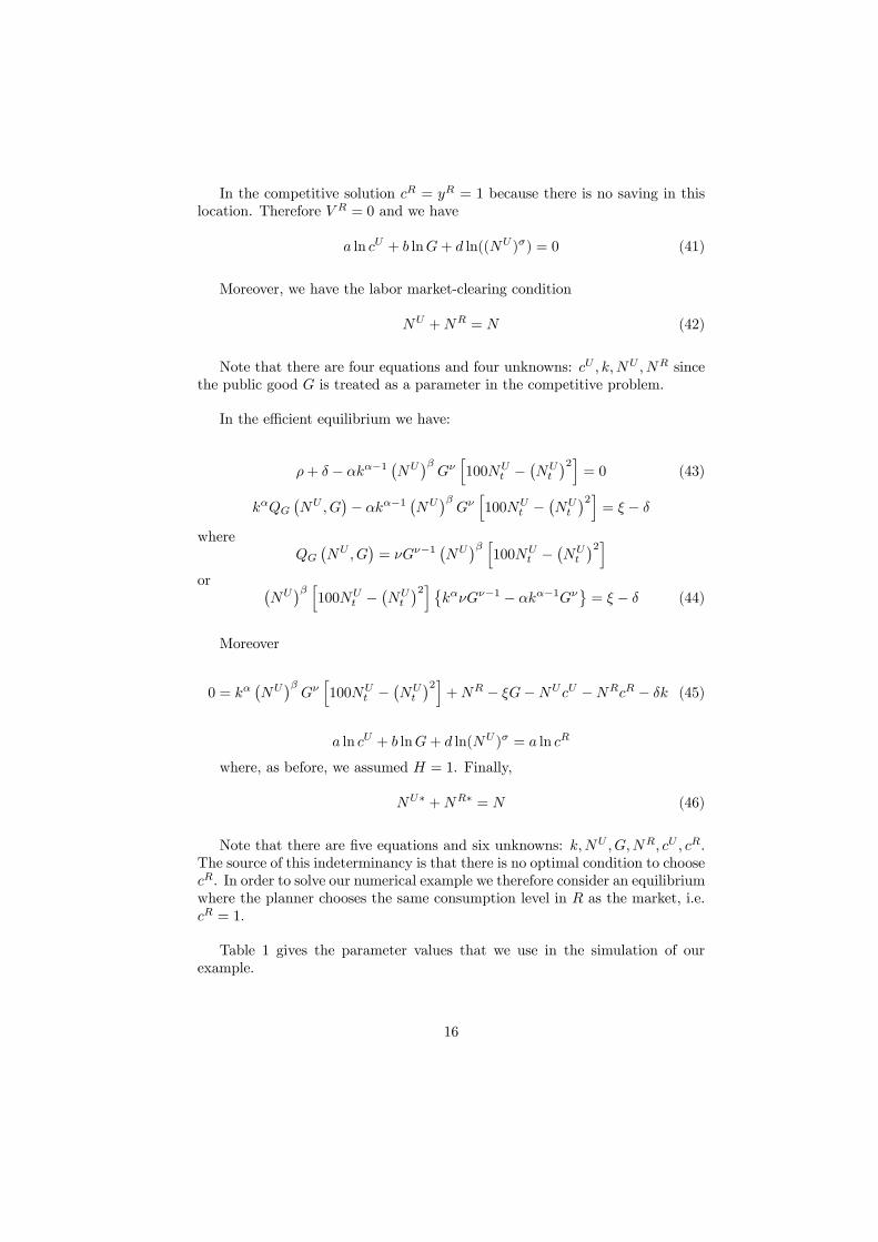
Note that there are five equations and six unknowns: .

The source of this indeterminancy is that there is no optimal condition to choose

. In order to solve our numerical example we therefore consider an equilibrium

where the planner chooses the same consumption level in as the market, i.e.

= 1.

Table 1 gives the parameter values that we use in the simulation of our

example.

16

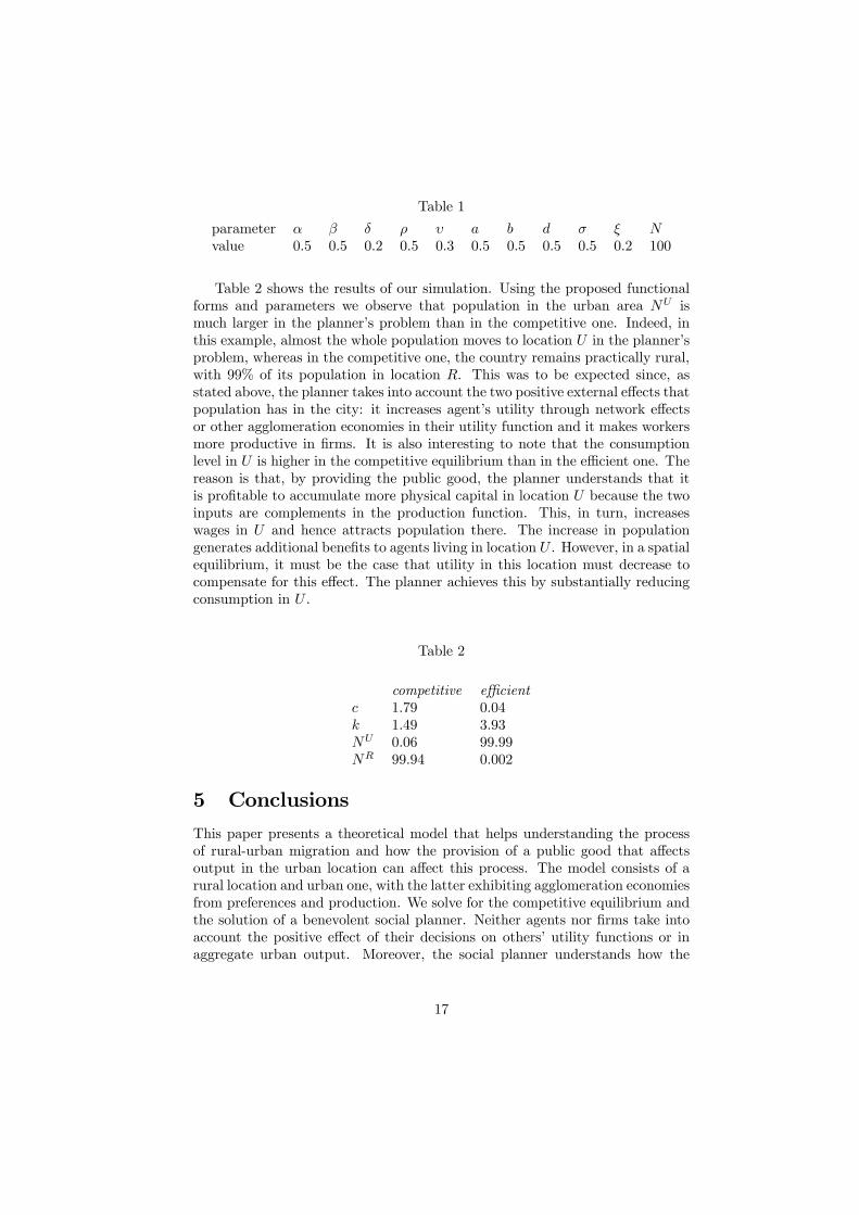
Table 1

parameter

value 0.5 0.5 0.2 0.5 0.3 0.5 0.5 0.5 0.5 0.2 100

Table 2 shows the results of our simulation. Using the proposed functional

forms and parameters we observe that population in the urban area is

much larger in the planner’s problem than in the competitive one. Indeed, in

this example, almost the whole population moves to location in the planner’s

problem, whereas in the competitive one, the country remains practically rural,

with 99% of its population in location . This was to be expected since, as

stated above, the planner takes into account the two positive external effects that

population has in the city: it increases agent’s utility through network effects

or other agglomeration economies in their utility function and it makes workers

more productive in firms. It is also interesting to note that the consumption

level in is higher in the competitive equilibrium than in the efficient one. The

reason is that, by providing the public good, the planner understands that it

is profitable to accumulate more physical capital in location because the two

inputs are complements in the production function. This, in turn, increases

wages in and hence attracts population there. The increase in population

generates additional benefits to agents living in location . However, in a spatial

equilibrium, it must be the case that utility in this location must decrease to

compensate for this effect. The planner achieves this by substantially reducing

consumption in .

Table 2

competitive efficient

1.79 0.04

1.49 3.93

0.06 99.99

99.94 0.002

5 Conclusions

This paper presents a theoretical model that helps understanding the process

of rural-urban migration and how the provision of a public good that affects

output in the urban location can affect this process. The model consists of a

rural location and urban one, with the latter exhibiting agglomeration economies

from preferences and production. We solve for the competitive equilibrium and

the solution of a benevolent social planner. Neither agents nor firms take into

account the positive effect of their decisions on others’ utility functions or in

aggregate urban output. Moreover, the social planner understands how the

17

provision of a public good in the urban location interacts with these agglom-

erations. For these two reasons, the decentralized equilibrium in this model is

inefficient.

The model can be applied to interpret the evolution of urbanization in differ-

ent world regions, in particular South Asia, where the percentage of population

living in urban areas is puzzlingly low given the region’s income level. We show

that, from a theoretical point of view, the large rural population in these coun-

tries can be rationalized by policies that give incentives for workers to stay in

rural areas. For example, in the model, a lack of investment in the urban public

good discourages urban production and so it delays urbanization. Finally, al-

though this is not the focus of the paper, our model can also be used to study the

evolution of rural-urban consumption and income gaps over time and how they

may be affected by specific policies. While we agree with the view of Fujita et

al. (2001) that more empirical work is needed to guide policy makers on how to

deal with urbanization, we believe this research needs to go hand-in-hand with

sound theoretical frameworks that allows us to interpret and organize the data

in a clear way. The present paper can be read as a contribution toward gener-

ating more dynamics to understand the process of rural-urban transformation

and how different policies affect it.

18

References

[1] Anas, A., 1978. Dynamics of urban residential growth. Journal of Urban

Economics, 5, 66 -87.

[2] Arnott, R. 2007. Congestion tolling with agglomeration externalities. Jour-

nal of Urban Economics, 62:2, 187-203.

[3] Au, C-C., Henderson, J.V., 2006. Are Chinese cities too small? Review of

Economic Studies 73(3), 549-576.

[4] Becker, G.S, and Murphy, K.M., 1992. The division of labor, coordination

costs, and knowledge. Quarterly Journal of Economics 11-37.

[5] Black, D, Henderson J.V. 1999. The theory of urban growth. Journal of

Political Economy 107, 252-284

[6] Chan, J-Y., Yu, E.S.H., 2010. Imperfect capital mobility: A general ap-

proach to the two-sector Harris-Todaro model. Review of International

Economics 18(1), 81-94.

[7] Cuberes, D., 2009. A model of sequential city growth. The B.E. Journal of

Macroeconomics (Contributions), March, 9(1), Article 18.

[8] Duranton, G., Puga, D. 2001. Nursery cities: urban diversity, process inno-

vation, and the life cycle of products. American Economic Review, 91(5),

December, 1454-1477.

[9] Fujita, M., 1982. Spatial patterns of residential development. Journal of

Urban Economics 12, 22-52.

[10] Fuijta, M., Krugman, P.R., Venables, A.J., 2001. The Spatial Economy.

Cities, Regions, and International Trade. The MIT Press.

[11] Gillespie, F., 1983. Comprehending the slow pace of urbanization in

Paraguay. Economic Development and Cultural Change 31, 355-375.

[12] Harris, J., Todaro, M., 1970. Migration, unemployment and development:

A two-sector analysis. American Economic Review 60, 126-142.

[13] Helsley, R.W., Strange, W.C., 1990. City formation with commitment. Re-

gional Science and Urban Economics 24, 373-390.

[14] Henderson, J.V., 1974. The sizes and types of cities. American Economic

Review, LXIV, 640-656.

[15] Henderson, J.V., 1988. Urban Development: Theory, Fact and Illusion,

Oxford: Oxford University Press.

[16] Henderson, J.V., Ioannides, Y.M., 1981. Aspects of growth in a system of

cities. Journal of Urban Economics 10, 117-139.

19

[17] Henderson, J.V., Kuncoro, A., 1996. Industrial centralization in Indonesia.

World Bank Economic Review, 10, 513-540.

[18] Henderson, J.V., Venables, A.J., 2009. Dynamics of city formation. Review

of Economic Dynamics 12(2), April, 233-254.

[19] Henderson, J.V., Wang, H.G., 2005. Aspects of the rural-urban transfor-

mation of countries. Journal of Economic Geography 5(1), 23-42.

[20] Henderson, J.V., Wang, H.G., 2007. Urbanization and city growth: The

role of institutions. Regional Science and Urban Economics 37(3), May,

283-313.

[21] Ioannides, Y., 1994. Product differentiation and economic growth in a sys-

tem of cities. Regional Science and Urban Economics 24, 461-484.

[22] Jefferson, G., Singhe, I., 1999. Enterprise Reform in China: Ownership

Transition and Performance. New York: Oxford University Press.

[23] Kanemoto, Y., 1980. Externality, migration, and urban crises. Journal of

Urban Economics, 8(2), September, 150-164.

[24] Lee, S.-K., Choe S.-C., 1990. Changing location patterns of industry and

urban decentralization policies in Korea. in J.K. Kwon (ed.), Korean Eco-

nomic Development. Santa Barbara, California: Greenwood Press.

[25] Miyao, T., 1981 Dynamic analysis of the urban economy. New York: Aca-

demic Press.

[26] Moretti, E., 2004. Human Capital Externalities in Cities, Handbook of

Urban and Regional Economics,North

Holland-Elsevier.

[27] Neary, J.P, 1981. On the Harris-Todaro model with intersectoral capital

mobility. Economica 48, August, 219-234.

[28] Neary, J.P, 1988. Stability of the mobile-capital Harris-Todaro model: Some

further results. Economica 55:217, February, 123-127.

[29] Palivos, T., Wang, P., 1996. Spatial agglomeration and endogenous growth.

Regional Science and Urban Economics 26(6), December, 645-669.

[30] Riadh, B.J., 1998. Rural-urban migration: On the Harris-Todaro model.”

Working paper.

[31] Richardson, H. (1987), “The Costs of Urbanization: A Four Country Com-

parison." Economic Development and Cultural Change, 33, 561-580.

[32] Rosenthal, S. S. and W. C. Strange (2003), "Geography, Industrial Orga-

nization, and Agglomeration," Review of Economics and Statistics, 85:2,

377-393

20

[33] Venables, A. J. (2007), "Evaluating Urban Transport Improvements," Jour-

nal of Transport Economics and Policy, 41:2, pp. 173-188

21

Appendix

Law of motion of population in location

From the population FOC in (equation (19)) we have

−ΦΦ0 + 1[ ()

¡

¢− ]− 2 = 0

Using 1 = 2

−ΦΦ0 = 1£1− ()

¡

¢+

¤Taking logs

−+ ln+ lnΦ + lnΦ0 = ln1 + ln£1− ()

¡

¢+

¤and differentiating with respect to time

−+Φ

Φ+

Φ0

Φ0=

1

1+

[1− ()( )+ ]

1− ()

¡

¢+

Now note that

Φ( Φ(

))

= Φ

+ ΦΦΦ

0

Moreover

£1− ()

¡

¢+

¤

= − 0()

¡

¢− ()

¡

¢

− ()

¡

¢ +

So using (25) again we end up with

−+ Φ + ΦΦΦ

0

Φ+

Φ00

Φ0=

− 0()¡

¢+

− 0()

¡

¢1− ()

¡

¢+

− ()

¡

¢

1− ()

¡

¢+

− ()

¡

¢ +

1− ()

¡

¢+

22

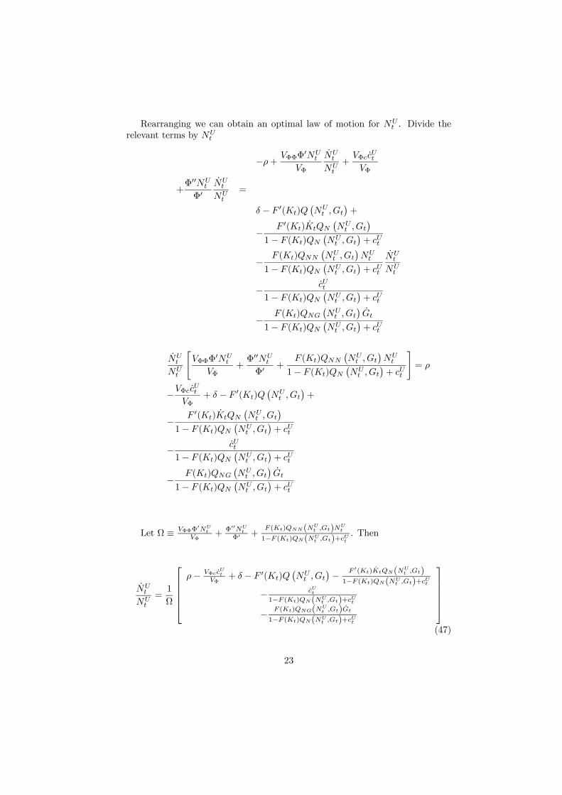
Rearranging we can obtain an optimal law of motion for . Divide the

relevant terms by

−+ ΦΦΦ0

Φ

+Φ

Φ

+Φ00

Φ0

=

− 0()¡

¢+

− 0()

¡

¢1− ()

¡

¢+

− ()

¡

¢

1− ()

¡

¢+

−

1− ()

¡

¢+

− ()

¡

¢

1− ()

¡

¢+

"ΦΦΦ

0

Φ+Φ00

Φ0+

()

¡

¢

1− ()

¡

¢+

#=

−Φ

Φ+ − 0()

¡

¢+

− 0()

¡

¢1− ()

¡

¢+

−

1− ()

¡

¢+

− ()

¡

¢

1− ()

¡

¢+

Let Ω ≡ ΦΦΦ0

Φ+Φ00

Φ0 + ()(

)

1− ()( )+

. Then

=1

Ω

⎡⎢⎢⎢⎢⎣− Φ

Φ+ − 0()

¡

¢− 0()( )

1− ()( )+

− 1− ()(

)+

− ()( )

1− ()( )+

⎤⎥⎥⎥⎥⎦(47)

23