Embed Size (px)
Citation preview
A DYNAMICAL SYSTEM ASSOCIATED WITH NEWTON’SMETHOD FOR PARAMETRIC APPROXIMATIONS OF CONVEX
MINIMIZATION PROBLEMS∗
F. ALVAREZ D.† AND J.M. PEREZ C.‡
Abstract. We study the existence and asymptotic convergence when t → +∞ for the trajectoriesgenerated by
∇2f(u(t), ε(t))u(t) + ε(t)∂2f
∂ε∂x(u(t), ε(t)) +∇f(u(t), ε(t)) = 0
where f(·, ε)ε>0 is a parametric family of convex functions which approximates a given convexfunction f we want to minimize, and ε(t) is a parametrization such that ε(t) → 0 when t → +∞.This method is obtained from the following variational characterization of Newton’s method
(P εt ) u(t) ∈ Argminf(x, ε(t))− e−t〈∇f(u0, ε0), x〉 : x ∈ H
where H is a real Hilbert space. We find conditions on the approximating family f(·, ε) and theparametrization ε(t) to ensure the norm convergence of the solution trajectories u(t) towards a par-ticular minimizer of f . The asymptotic estimates obtained allow us to study the rate of convergenceas well. The results are illustrated through some applications to barrier and penalty methods forlinear programming, and to viscosity methods for an abstract non-coercive variational problem.Comparisons with the steepest descent method are also provided.
Key words. Convex minimization, approximate methods, continuous methods, evolution equa-tions, existence, optimal trajectory, asymptotic analysis.
AMS subject classifications. 34G20, 34A12, 34D05, 90C25, 90C31
1. Introduction. Newton’s method for solving a smooth optimization problemon a real Hilbert space H
(P ) minf(x) : x ∈ H,
is based on sequentially minimizing the quadratic expansion of f , that is to say, themethod recursively computes
uk+1 = uk −∇2f(uk)−1∇f(uk).(1)
It is well known that under suitable assumptions (f ∈ C3 and ∇2f(x) positive definiteat a local minimizer x) and starting sufficiently close to x, the iterative scheme (1)is well defined and converges to x quadratically: |uk+1 − x| ≤ C|uk − x|2. However,when the method is far from the solution there is no guarantee of convergence andone must introduce an appropriate step size λk > 0, leading to
uk+1 − uk
λk= −∇2f(uk)−1∇f(uk),
which can be interpreted as an explicit discrete scheme for the continuous Newton’smethod,
∇2f(u(t))u(t) +∇f(u(t)) = 0.(2)
∗Partially supported by Fondecyt 1961131.†Supported by the CEE grant CI1-CT94-01115. Universidad de Chile, Casilla 170/3 Correo 3,
Santiago, Chile. e-mail:[email protected]‡Supported by funds from Fundacion Andes. Pedro Montt 147, Penablanca, Villa Alemana, Chile.
e-mail:[email protected]
1
2 F. ALVAREZ AND J.M. PEREZ
It is easy to check that every solution of (2) satisfies
d
dt[∇f(u(t))] = −∇f(u(t))
and therefore
∇f(u(t))− e−t∇f(u0) = 0.(3)
When the function f is convex, the latter is equivalent to
u(t) ∈ Argminf(x)− e−t〈∇f(u0), x〉 : x ∈ H(4)
providing a variational characterization for the Newton trajectory u(t) which does notrequire f to be of class C2 nor to have a nonsingular Hessian, and which makes senseeven for non smooth f ’s (replace∇f(u0) with any u∗0 ∈ ∂f(u0)). We consider this non-smooth extension of Newton’s method in §3, proving that u(t) is a descent trajectoryfor f which is defined for all t ≥ 0 (an interesting result even in the smooth case).Moreover, when f is strongly convex, we establish an exponential rate of convergencefor u(t) towards the unique minimizer of f .
When the function f is not strongly convex, and also when it presents an irregularbehavior because of non-smoothness or when it takes the value +∞ because of implicitconstraints, a classical approach is to replace f by a sequence of better behaved para-metric approximations (penalty methods, Tikhonov regularization, viscosity methods,etc.). More precisely, consider the one-parameter family of problems
(P ε) minf(x, ε) : x ∈ H
where for each ε > 0 the function f(·, ε) is a closed proper convex approximate con-verging to f when ε → 0. Numerical methods based on such parametric approximationschemes consist in solving (P ε) for an appropriate sequence εk converging to 0. Whenf(·, ε) is sufficiently smooth, a common practice is to use Newton’s method for sol-ving (P εk) up to a prescribed accuracy and then proceed to the next iteration withparameter εk+1.
Because of the usual increasing ill-conditioning of the Hessian matrix of theapproximating function f(·, ε), the convergence of the overall method requires a care-ful selection of the starting point for the Newton’s iterations as well as the sequence ofparameters εk, choices which are strongly interdependent. Unfortunately, no generaltheory is available in order to guide these choices. With the aim of contributing tothis issue, in §4 we consider the question in the simpler setting of a continuous methodcoupling Newton’s method with approximation schemes.
We observe that there is no standard way of coupling Newton’s method with anapproximation scheme. Possibly, the most straightforward alternative would be toconsider the non-autonomous differential equation
∇2f(u(t), ε(t))u(t) +∇f(u(t), ε(t)) = 0
where the parameter function ε(t) is a priori chosen so that it decreases to 0 whent → +∞. However, there is no reason for this method to be the most appropriate(not even the most natural) way of efficiently combining Newton’s method with anapproximation scheme. Taking into account the variational characterization (4) westudy in §4 a different generalization, namely
u(t) ∈ Argminf(x, ε(t))− e−t〈∇f(u0, ε0), x〉 : x ∈ H.(5)
CONTINUOUS NEWTON’S METHOD FOR CONVEX MINIMIZATION. 3
In the smooth case, this approach corresponds to the differential equation
∇2f(u(t), ε(t))u(t) + ε(t)∂2f
∂ε∂x(u(t), ε(t)) +∇f(u(t), ε(t)) = 0
whose associated vector field combines a Newton direction with an extrapolationterm that specifically takes into account the rate of change in the objective functiont → f(·, ε(t)).
We study the existence of solutions for (5) as well as their asymptotic behavior.In a general setting, we obtain a weak condition on the parametrization ε(t) ensur-ing the asymptotic convergence of the solution trajectories u(t) towards a particularsolution of the original problem (P ), giving at the same time an estimate of the rateof convergence. We illustrate the general results through some examples in the set-ting of barrier and penalty methods for linear programming, as well as for Tikhonovregularization methods.
We compare our results with those obtained for the steepest descent method (see[3]). To this end we include a short discussion of this method in the preliminarysection §2, for which we provide a new convergence proof for the non-parametric case.
In order to handle with the problem of the increasing ill-conditioning of Hessianoperator of the parametric approximation, we shall see in §5 how in certain cases anappropriate rescaling of the approximate problem may be used to obtain an uniformstrongly convex approximate scheme.
2. Preliminaries.
2.1. Basic assumptions. Throughout this paper we shall consider an abstractoptimization problem of the form
(P ) minf(x) : x ∈ H
where H is a real Hilbert space and f : H → IR ∪ +∞ is a closed proper convexfunction. The set of optimal solutions of (P ) is denoted Argmin f and we assumethroughout that
(H0) the optimal set Argmin f is nonempty and bounded.
This holds for instance when f is coercive (i.e. f has bounded level sets). Werecall that according to Moreau’s theorem, the latter is equivalent to finiteness andcontinuity of the Fenchel conjugate f∗ at x∗ = 0.
We say that f is strongly convex if there exists β > 0 such that
f(x) + 〈x∗, y − x〉+β
2|y − x|2 ≤ f(y),
for all x, y ∈ H and x∗ ∈ ∂f(x). Equivalently, f is strongly convex when its sub-differential operator is strongly monotone, that is to say, there exists β > 0 suchthat
(H1) if x∗ ∈ ∂f(x) and y∗ ∈ ∂f(y) then 〈x∗ − y∗, x− y〉 ≥ β|x− y|2
If f is strongly convex then f is strictly convex and coercive. In particular, there existsa unique point x solution of (P ). A weaker condition is the strong monotonicity overbounded sets,
(H2)∀K > 0, ∃βK > 0 s.t. ∀x, y ∈ B(0,K), if x∗ ∈ ∂f(x) and y∗ ∈ ∂f(y)
then 〈x∗ − y∗, x− y〉 ≥ βK |x− y|2
4 F. ALVAREZ AND J.M. PEREZ
We remark that in this case f is also strictly convex but may fail to satisfy (H0). As amatter of fact, in this case there is no guarantee of existence of an optimal solution. Inthe finite dimensional case, if f ∈ C2(IRn; IR) is such that the Hessian matrix ∇2f(x)is positive definite for all x ∈ IRn, then (H2) is satisfied and the parameter βK is alower bound for the eigenvalues of the matrix ∇2f(x) over B(0,K).
Together with the original problem (P ) we shall consider the parametric family
(P ε) minf(x, ε) : x ∈ H
where for each ε > 0, f(·, ε) is a closed proper convex function approximating f .Very often the function f(·, ε) may be chosen so that it enjoys good properties suchas coercivity and strong convexity and therefore the approximate problem (P ε) iswell posed in existence and uniqueness. We shall assume throughout that (P ε) has aunique solution which we denote x(ε), and more precisely we suppose that
(H3)there exists a unique path x(ε) of optimal solutions of (P ε) whichconverge in norm towards an optimal point x ∈ Argmin f when ε → 0.
Variational notions of convergence for sequences of functions provide an appro-priate setting for studying the convergence of the optimal solutions of approximateschemes as the previous one. For instance, assuming that the following Mosco-epi-limit holds
f = epi− limε→0
f(·, ε),
and under appropriate compacity assumptions, the optimal value min f(·, ε) convergesto min f and every limit point of the optimal path x(ε) : ε → 0 is an optimal solutionof (P ). The latter does not ensure the convergence of the optimal path unless (P ) hasa unique solution. However, with a more specific analysis, the validity of (H3) has beenestablished for many approximate schemes: for viscosity approximation methods seeTikhonov and Arsenine [16], Attouch [1] and references therein; for interior-point andpenalty methods in convex and linear programming see Megiddo [14], Gonzaga [12],Cominetti and San Martin [9], Fiacco [10] and Auslender, Cominetti and Haddou[5]; for an abstract approach based on epi-convergence and scaling see Attouch [2]and Torralba [17], as well as §5. In all these cases, the limit point x has remarkablevariational properties which make its computation interesting by its own.
2.2. Steepest descent method. For the sake of comparison with the results tobe presented for the Newton method, we briefly recall in this section the convergenceproperties of the steepest descent method for the problem (P ) as well as its couplingwith the approximate scheme (P ε).
Let us begin with the steepest descent differential inclusion
(SD;u0)
u(t) + ∂f(u(t)) 3 0u(0) = u0.
An absolutely continuous function u : [0,+∞) → H is a solution of (SD;u0) ifu(0) = u0 and the above inclusion is satisfied almost everywhere in [0,+∞). It isa classical result that when the minimum of f is attained, every solution u(t) of(SD;u0), weakly converges to an element u∞ ∈ Argmin f as t → +∞ (see Brezis[6, 7], Bruck [8]). When (P ) has multiple optimal solutions, the limit point may
CONTINUOUS NEWTON’S METHOD FOR CONVEX MINIMIZATION. 5
depend on the initial condition u0 and it may be difficult to characterize (see Lemaire[13] for results along these lines).
When f is strongly convex, it is possible to estimate the rate of convergence of thetrajectory u(t) (see Brezis [6, Theorem 3.9]). In the following proposition, we presenta slight variant of this result which assumes only the strong convexity over boundedsets, and which also provides an estimate for the rate of convergence of the functionvalues.
Proposition 2.1. Let f be a coercive convex function satisfying (H2), and letx be the unique minimizer of f . If u : [0,+∞) → H is a solution of (SD;u0), thenthere exists β > 0 such that for all t > 0,
f(u(t))−min f ≤ (f(u0)−min f)e−βt,
and
|u(t)− x| ≤√
2β
(f(u0)−min f)e−β2 t.
Proof. Let v(t) := f(u(t)) −min f . It is known [6, Theorem 3.6 and lemma 3.3]that when
u0 ∈ domf = x ∈ H : f(x) < +∞
then f(u(t)) is an absolutely continuous function. Moreover, we have
d
dtf(u(t)) =< x∗, u(t) >
for all x∗ ∈ ∂f(u(t)) and almost everywhere in [0,+∞). In particular we obtainv(t) = −|u(t)|2, so that v(t) is non-increasing and since f is coercive the trajectoryu(t) stays bounded as t → +∞.
Let us assume that for all t ≥ 0 we have u(t) 6= x (otherwise the result is obvious).Then, using the convexity inequality 〈x∗, x− u(t)〉 ≤ f(x)− f(u(t)) together with
|x∗| ≥ 1|u(t)− x|
〈x∗, u(t)− x〉,
it follows that
v(t) ≤ |x∗||u(t)− x|
[f(x)− f(u(t))] = − |x∗||u(t)− x|
v(t),
when x∗ ∈ ∂f(u(t)). Taking a suitable constant K such that |u(t)| ≤ K for allt ≥ 0 and |x| ≤ K, using (H2) and the facts that 0 ∈ ∂f(x) and v(t) ≥ 0, weobtain v(t) ≤ −βv(t) with β := βK . The conclusions follow at once by integratingthe inequality v(t) ≤ −βv(t), and then using the strong convexity inequality f(x) +β2 |u(t)− x|2 ≤ f(u(t)). 2
Remark. Using a special notion of weak solution for (SD;u0) (Brezis [6]), it ispossible to take in the previous proposition u0 ∈ Adh(domf).
This result shows that when f is strongly convex, the steepest descent method hasa very good behavior, converging towards the solution of (P ) at an exponential rate.However, these assumptions do not hold in many interesting situations, particularly
6 F. ALVAREZ AND J.M. PEREZ
when the original problem (P ) has multiple solutions or when the function f is notregular or finite. This led Attouch and Cominetti [3] to consider the coupling of thesteepest descent method with approximation schemes in the following way
(DADA;u0)
u(t) + ∂f(u(t), ε(t)) 3 0u(0) = u0.
where the function ε : [0,+∞) → IR+ is strictly positive and decreasing to 0 witht → +∞.
Roughly speaking, if ε(t) converges sufficiently fast to 0, one expects that thesolution trajectories of (DADA) behave like the solutions of (SD) which can beconsidered as a limit equation for (DADA) (with ε(t) = 0). As a matter of fact,under suitable hypothesis, it was proved by Furuya, Miyashiba and Kenmochi [11]that in this case the trajectory u(t) converges towards an optimal solution of (P ).
On the other hand, it has been proved by Attouch and Cominetti [3] that whenε(t) converges to 0 sufficiently slow, then u(t) asymptotically approaches the optimaltrajectory x(ε(t)) and therefore it is attracted towards x. The speed of convergenceof ε(t) is measured in terms of the strong convexity parameter β(ε) of f(·, ε), namely,the condition
(H4) 〈∂f(x, ε)− ∂f(y, ε), x− y〉 ≥ β(ε)|x− y|2
implies that (see [3] for details) for all t ≥ t0 ≥ 0
|u(t)− x(ε(t))| ≤ Ce−(E(t)−E(t0)) − e−E(t)
∫ t
t0
eE(s)
∣∣∣∣dx
dε(ε(s))
∣∣∣∣ ε(s)ds(6)
where C := |u0 − x(ε(t0))| and E(t) =∫ t
0β(ε(s))ds. It follows that u(t) converges
strongly towards x whenever ∫ +∞
0
β(ε(s))ds = +∞(7)
and either (a) or (b) below hold:
(a)∫ ε0
0
∣∣∣∣dx
dε
∣∣∣∣ ds < +∞,
(b) limt→+∞
∣∣∣∣dx
dε(ε(t))
∣∣∣∣ ε(t)β(ε(t))
= 0.
Remark. When f(·, ε) = f(·) for all ε > 0 then (DADA) correspond to (SD)with f strongly convex. In this case, the estimate (6) implies
|u(t)− x| ≤ |x0 − x|e−βt
which is in fact the estimate obtained by Brezis [6].
It is quite natural to investigate the coupling of approximation schemes withother descent methods, particularly a second order method such as Newton’s. In thenext section we study a variational characterization of the Newton trajectory whichleads naturally to a dynamical method coupling Newton’s method with approximationschemes.
CONTINUOUS NEWTON’S METHOD FOR CONVEX MINIMIZATION. 7
3. A variational characterization of the Newton trajectory. Let us goback to the original problem (P ) and consider the following family of problems
(Pt) u(t) ∈ Argminf(x)− e−t〈x∗0, x〉 : x ∈ H,
where x∗0 ∈ ∂f(u0) is fixed. The optimality condition for (Pt) is
∂f(u(t))− e−tx∗0 3 0
which is the non-smooth version of equation (3), so that (Pt) can be considered asa non-smooth extension of the Newton method. As a matter of fact, we will provein §3.1 that under appropriate assumptions the trajectory u(t) coincides with theNewton trajectory.
Proposition 3.1. If f is coercive then the optimal set of (Pt) is non-empty andbounded for all t > 0.
Proof. Consider the function g(x, t) := f(x) − e−t〈x∗0, x〉. For all x∗ ∈ H theFenchel conjugate of g(·, t) is given by
g∗(x∗, t) = supx∈H
〈x∗, x〉 − g(x, t) = f∗(x∗ + e−tx∗0).
Since x∗0 ∈ ∂f(u0) it follows that f∗ is finite at x∗0. On the other hand, our assumptionon f and Moreau’s theorem ensure that f∗ is finite and continuous at 0, and there-fore the same holds at each point in the segment [0, x∗0). Hence g∗(·, t) is finite andcontinuous at 0 for all t > 0 and the conclusion follows by using Moreau’s theoremonce again. 2
Since u0 solves (P0), applying the last proposition one may select an optimaltrajectory u : [0,+∞) → H with u(0) = u0. If the function f is strictly convex, thenthis trajectory u(t) is unique. Having established conditions for the existence anduniqueness of u(t), the question that comes out is its behavior when t → +∞.
Proposition 3.2. Let u : [0,+∞) → H be a trajectory of solutions of (Pt).Then u(·) is a descent trajectory for f , that is to say
∀t ≥ 0,∀h ≥ 0 f(u(t + h)) ≤ f(u(t)).
In particular, if f is coercive then u(t) stays bounded as t → +∞.Proof. Since u(t + h) is an optimal solution for (Pt+h), we have
f(u(t + h))− e−(t+h)〈x∗0, u(t + h)〉 ≤ f(u(t))− e−(t+h)〈x∗0, u(t)〉
and therefore
f(u(t + h))− f(u(t)) ≤ e−(t+h)〈x∗0, u(t + h)− u(t)〉.(8)
On the other hand, the optimality of u(t) for (Pt) implies that e−tx∗0 ∈ ∂f(u(t)) sothat
e−t〈x∗0, u(t + h)− u(t)〉 ≤ f(u(t + h))− f(u(t))
which combined with (8) gives
f(u(t + h))− f(u(t)) ≤ e−h[f(u(t + h))− f(u(t))]
8 F. ALVAREZ AND J.M. PEREZ
and therefore f(u(t + h))− f(u(t)) ≤ 0. 2
With the previous results we may now stateProposition 3.3. Assume that f is coercive and let u(t) be an optimal trajectory
for (Pt). Then
limt→+∞
f(u(t)) = min f
and every weak limit point of the trajectory u(t) : t → +∞ belongs to the optimalset Argmin f .
Moreover, if f satisfies (H2) then there exists a constant C > 0 such that
|u(t)− x| ≤ Ce−t
where x is the unique optimal solution of (P ).Proof. The optimality condition ∂f(u(t))− e−tx∗0 3 0 can be equivalently stated
as
f(u(t)) + f∗(e−tx∗0) = e−t〈x∗0, u(t)〉.(9)
By Moreau’s theorem, f∗ is finite and continuous at 0, while the previous propositionand the coercivity of f implies that u(t) stays bounded as t → +∞. Passing to thelimit in (9) we get
limt→+∞
f(u(t)) = −f∗(0) = infx∈H
f(x).
Since u(t) stays bounded as t → +∞ it has weak limit points, and the weak lowersemi-continuity of f together with the convergence of the optimal values, imply thatthese limit points minimize f .
When f satisfies (H2), recalling that e−tx∗0 ∈ ∂f(u(t)) and 0 ∈ ∂f(x), we obtain
〈e−tx∗0, u(t)− x〉 ≥ βK |u(t)− x|2
for a suitable constant K > 0, and therefore
|u(t)− x| ≤ 1βK
e−t|x∗0|,
and the conclusion follows with C = |x∗0|/βK . 2
3.1. Equivalence with the continuous Newton’s method. When moti-vating the study of the family of the problems (Pt)t≥0 in §1, we started from thecontinuous Newton method
(CN ;u0)∇2f(u(t))u(t) +∇f(u(t)) = 0u(0) = u0,
and we observed that every solution was an optimal trajectory for (Pt).The following simple result establishes that the converse holds under suitable dif-
ferentiability assumptions. Therefore, the previous results extend to the non-smoothsetting those obtained for (CN ;u0) by Aubin and Cellina [4] using the viability theoryfor differential inclusions.
CONTINUOUS NEWTON’S METHOD FOR CONVEX MINIMIZATION. 9
Proposition 3.4. Let f ∈ C2(H; IR) be strongly convex function. Then a func-tion u : [0,+∞) → H is an optimal trajectory for (Pt) if and only if it is the globalsolution of the differential equation (CN ;u0).
Proof. We just prove the “only if” part. Let u : [0,+∞) → H be the optimaltrajectory for (Pt), characterized by the optimality condition
∇f(u(t))− e−t∇f(u0) = 0.(10)
Since f ∈ C2(H; IR) and ∇2f(x) is invertible for all x ∈ H (Lax-Milgram theorem)we can apply the Implicit Function Theorem to (10) in order to conclude that u(·) isdifferentiable for all t ≥ 0. Differentiating (10) with respect to t, we obtain
∇2f(u(t))u(t) + e−t∇f(u0) = 0,
and using the optimality condition once again we get
∇2f(u(t))u(t) +∇f(u(t)) = 0,
so that u(·) is a solution of (CN ;u0). 2
Corollary 3.5. Let f ∈ C2(H; IR) be strongly convex. Then for all u0 ∈ Hthere exists a unique u : [0,+∞) → H solution trajectory of (CN ;u0), which is adescent trajectory for f and satisfies
|u(t)− x| ≤ Ce−t
where C is a constant and x is the unique minimizer of f .
4. Approximation and continuous Newton’s method. We have seen in theprevious section that under strong convexity the convergence of Newton’s method isvery fast. Unfortunately, strong convexity is a drastic restriction which does not holdin many interesting optimization problems, particularly when there exist multipleoptimal solutions. A typical and very important case is linear programming.
As mentioned in §1, the main idea to be developed hereafter is to combine thecontinuous Newton method with approximation schemes in which the original problem(P ) is replaced by a sequence of well-posed strongly convex minimization problemsminf(x, ε) : x ∈ H. Our previous analysis was mainly based on the variationalcharacterization of the Newton trajectory. Hence we are naturally led to consider thefollowing family of optimization problems
(P εt ) u(t) = Argminf(x, ε(t))− e−t〈x∗0, x〉 : x ∈ H
where x∗0 ∈ ∂f(u0, ε0) and the functions ε(t) and f(·, ε) are chosen as in §2.1.Although much of the subsequent analysis remains valid in a non-smooth setting,
we are specially interested in obtaining a differential equation equivalent to (P εt ).
Therefore, we shall assume that the approximating function f(x, ε) is as smooth asrequired.
The optimality condition for (P εt ) is
∇f(u(t), ε(t))− e−t∇f(u0, ε0) = 0.
If the solution trajectory u(t) exists and is smooth, we can differentiate this stationa-rity condition in order to obtain
∇2f(u(t), ε(t))u(t) + ε(t)∂2f
∂ε∂x(u(t), ε(t)) + e−t∇f(u0, ε0) = 0,
10 F. ALVAREZ AND J.M. PEREZ
from which we derive the differential problem
(ACN) ∇2f(u(t), ε(t))u(t) + ε(t)∂2f
∂ε∂x(u(t), ε(t)) +∇f(u(t), ε(t)) = 0
to which we shall refer as the Approximate Continuous Newton method. This dynami-cal system combines a Newton correction term leading the trajectory u(t) towards theexact minimizer x(ε(t)) of f(·, ε(t)), with an extrapolation term anticipating changesin the target point x(ε(t)).
Remark. An alternative to (P εt ) would be to introduce a one-to-one differen-
tiable function η : [0,+∞) → [0,+∞) as follows
u(t) = Argminf(x, ε(t))− e−η(t)〈∇f(u0, ε0), x〉 : x ∈ H,
which leads to the differential equation
∇2f(u(t), ε(t))u(t) + ε(t)∂2f
∂ε∂x(u(t), ε(t)) + η(t)∇f(u(t), ε(t)) = 0.(11)
Introducing the change of variables t = θ(s) with θ = η−1, and defining v(s) :=u(θ(s)), (11) is transformed into
∇2f(v(s), ε(θ(s)))v(s) +d
ds(ε(θ(s)))
∂2f
∂ε∂x(v(s), ε(θ(s))) +∇f(v(s), ε(θ(s))) = 0,
which is (ACN) with a reparametrized approximating scheme. We will use a re-parametrization of this kind in §5.
4.1. Existence and asymptotic behavior of the trajectories. We begin bynoting that the unique minimizer x(ε) of f(·, ε) can be characterized as the uniquesolution of
∇f(x(ε), ε) = 0.
When ∇2f(x(ε), ε) is positive definite, the implicit function theorem ensures that thecurve ε → x(ε) is differentiable and satisfies
∇2f(x(ε), ε)dx
dε(ε) +
∂2f
∂ε∂x(x(ε), ε) = 0.
Therefore, if the initial condition is u0 = x(ε0) then u(t) = x(ε(t)) is the uniquesolution of (ACN).
We shall prove in the sequel that when the initial condition u0 does not lie onthe optimal trajectory, the solution trajectory u(t) will nevertheless approach x(ε(t)),from which we may deduce its convergence towards x. As a by-product we obtain auseful estimate for the rate of convergence.
4.1.1. The strongly convex case. For simplicity, we shall assume in the follo-wing that the effective domain of the approximating function is a constant open set,that is to say, there exists an open set Ω ⊂ H such that
Ω = domf(·, ε) = x ∈ H : f(x, ε) < +∞
for all ε > 0.
CONTINUOUS NEWTON’S METHOD FOR CONVEX MINIMIZATION. 11
Theorem 4.1. Let us consider an approximate family f(·, ε)ε>0 such thatf(·, ·) ∈ C2(Ω × (0, ε0]; IR), where Ω = domf(·, ε) for all ε > 0. If f(·, ε) is stronglyconvex with parameter β(ε) then
(i) For every initial condition u0 ∈ Ω, there exists a unique u : [0,+∞) → Ωsolution trajectory for (ACN) which satisfies
|u(t)− x(ε(t))| ≤ |∇f(u0, ε0)|e−t
β(ε(t))(12)
where x(ε) is the optimal solution of (P ε).(ii) If (H3) is satisfied and
limt→+∞
etβ(ε(t)) = +∞(13)
then
limt→+∞
u(t) = limt→+∞
x(ε(t)) = x.
Proof. The proof uses the same techniques of the non-parametric case. To prove(i), we study the existence and uniqueness of an optimal trajectory for the variationalcharacterization
(P εt ) u(t) = Argminf(x, ε(t))− e−t〈∇f(u0, ε0), x〉 : x ∈ H.
Since f(·, ε) is strongly convex, then the function
g(x, t) := f(x, ε(t))− e−t〈∇f(u0, ε0), x〉
is also strongly convex with the same parameter β(ε). So, there exists a unique u(t)optimal solution (P ε
t ) which belongs to Ω. Moreover, applying the Implicit FunctionTheorem to the optimality condition of (P ε
t ), we conclude that u : [0,+∞) → Ωis differentiable and is a solution trajectory for (ACN). Noting that a solution of(ACN) is a optimal trajectory for (P ε
t ), the uniquess for (ACN) follows.For the estimate, it is enough to notice that from the strong monotonicity property
it follows that
〈∇f(u(t), ε(t)), u(t)− x(ε(t))〉 ≥ β(ε(t))|u(t)− x(ε(t))|2,
so that
|u(t)− x(ε(t))| ≤ e−t
β(ε(t))|∇f(u0, ε0)|.
Since (ii) is a direct consequence of (i) the proof is complete.2
Note that we have made no assumptions on the optimal path x(ε) except its con-vergence towards x. The latter is a distinguishing feature of the approximate New-ton’s method (ACN) with respect to known results for the steepest descent method(DADA) (see conditions (a) and (b) in §2.2). Moreover, equation (13) provides a rel-atively weak condition on the parameter function ε(t) which ensures that the solutiontrajectories of (ACN) asymptotically approaches the optimal trajectory x(ε(t)). Weshall see in the following examples that condition (13) is much weaker than the basichypothesis (7) needed for convergence in the steepest descent method.
12 F. ALVAREZ AND J.M. PEREZ
Before proceeding with these examples it is illustrative to compare (12) with thecorresponding estimate (6) for (DADA). Assume that the strong convexity propertyholds with parameter β(ε) = ε and also that the optimal path satisfies∣∣∣∣dx
dε(ε)
∣∣∣∣ ≤ C0
for some constant C0, which implies the finite length of the optimal path (see condition(a)). If we have ∫ +∞
0
ε(s)ds = +∞
then the solution uD(t) of (DADA) norm converges to x.Take for instance ε(t) = (1−α)(1+ t)−α with 0 < α < 1. After a careful analysis
of (6), it is possible to prove that asymptotically,
|uD(t)− x(ε(t))| ≤ C
tα(14)
for a suitable constant C and t large enough (see [3]). Denote by uN (t) the corres-ponding solution for (ACN), then (12) directly becomes
|uN (t)− x(ε(t))| ≤ |∇f(u0, ε0)|(1− α)
(1 + t)α
et
which is sharper than (14).If we take ε(t) = 1/(1 + t) then asymptotically (see [3]),
|uD(t)− x(ε(t))| ≤ Cln(t)
t
for certain C > 0 and t large, while for the solution of (ACN) we have
|uN (t)− x(ε(t))| ≤ |∇f(u0, ε0)|1 + t
et
which converges to 0 much faster than ln(t)/t.The sharper estimates obtained with (ACN) must be balanced with the simpler
form of (DADA) and with the extra effort involved in the computation of the inverseof the Hessian in (ACN).
Example 1. Log-barrier in linear programming.With the linear program
(LP ) minc′x : Ax ≤ b
it is associated the function
f(x) =
c′x if Ax ≤ b+∞ otherwise
The log-barrier approximation of f is given by
f(x, ε) = c′x− εm∑
i=1
ln(bi − a′ix).(15)
CONTINUOUS NEWTON’S METHOD FOR CONVEX MINIMIZATION. 13
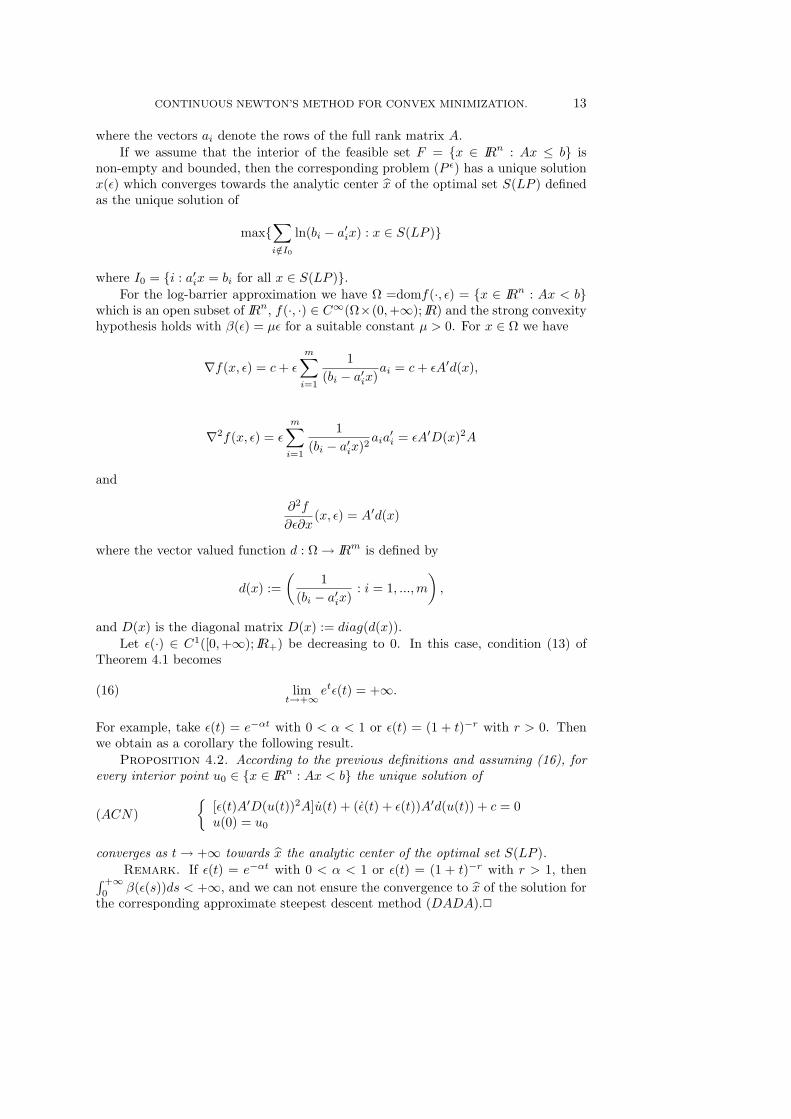
where the vectors ai denote the rows of the full rank matrix A.If we assume that the interior of the feasible set F = x ∈ IRn : Ax ≤ b is
non-empty and bounded, then the corresponding problem (P ε) has a unique solutionx(ε) which converges towards the analytic center x of the optimal set S(LP ) definedas the unique solution of
max∑i/∈I0
ln(bi − a′ix) : x ∈ S(LP )
where I0 = i : a′ix = bi for all x ∈ S(LP ).For the log-barrier approximation we have Ω =domf(·, ε) = x ∈ IRn : Ax < b
which is an open subset of IRn, f(·, ·) ∈ C∞(Ω×(0,+∞); IR) and the strong convexityhypothesis holds with β(ε) = µε for a suitable constant µ > 0. For x ∈ Ω we have
∇f(x, ε) = c + εm∑
i=1
1(bi − a′ix)
ai = c + εA′d(x),
∇2f(x, ε) = εm∑
i=1
1(bi − a′ix)2
aia′i = εA′D(x)2A
and
∂2f
∂ε∂x(x, ε) = A′d(x)
where the vector valued function d : Ω → IRm is defined by
d(x) :=(
1(bi − a′ix)
: i = 1, ...,m)
,
and D(x) is the diagonal matrix D(x) := diag(d(x)).Let ε(·) ∈ C1([0,+∞); IR+) be decreasing to 0. In this case, condition (13) of
Theorem 4.1 becomes
limt→+∞
etε(t) = +∞.(16)
For example, take ε(t) = e−αt with 0 < α < 1 or ε(t) = (1 + t)−r with r > 0. Thenwe obtain as a corollary the following result.
Proposition 4.2. According to the previous definitions and assuming (16), forevery interior point u0 ∈ x ∈ IRn : Ax < b the unique solution of
(ACN)
[ε(t)A′D(u(t))2A]u(t) + (ε(t) + ε(t))A′d(u(t)) + c = 0u(0) = u0
converges as t → +∞ towards x the analytic center of the optimal set S(LP ).Remark. If ε(t) = e−αt with 0 < α < 1 or ε(t) = (1 + t)−r with r > 1, then∫ +∞
0β(ε(s))ds < +∞, and we can not ensure the convergence to x of the solution for
the corresponding approximate steepest descent method (DADA).2
14 F. ALVAREZ AND J.M. PEREZ
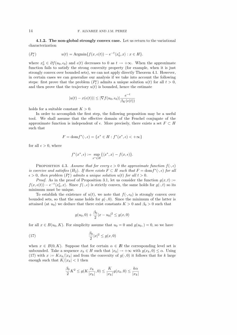
4.1.2. The non-global strongly convex case. Let us return to the variationalcharacterization
(P εt ) u(t) = Argminf(x, ε(t))− e−t〈x∗0, x〉 : x ∈ H.
where x∗0 ∈ ∂f(u0, ε0) and ε(t) decreases to 0 as t → +∞. When the approximatefunction fails to satisfy the strong convexity property (for example, when it is juststrongly convex over bounded sets), we can not apply directly Theorem 4.1. However,in certain cases we can generalize our analysis if we take into account the followingsteps: first prove that the problem (P ε
t ) admits a unique solution u(t) for all t > 0,and then prove that the trajectory u(t) is bounded, hence the estimate
|u(t)− x(ε(t))| ≤ |∇f(u0, ε0)|e−t
βK(ε(t))
holds for a suitable constant K > 0.In order to accomplish the first step, the following proposition may be a useful
tool. We shall assume that the effective domain of the Fenchel conjugate of theapproximate function is independent of ε. More precisely, there exists a set F ⊂ Hsuch that
F = domf∗(·, ε) = x∗ ∈ H : f∗(x∗, ε) < +∞
for all ε > 0, where
f∗(x∗, ε) := supx∗∈H
〈x∗, x〉 − f(x, ε).
Proposition 4.3. Assume that for every ε > 0 the approximate function f(·, ε)is coercive and satisfies (H2). If there exists F ⊂ H such that F = domf∗(·, ε) for allε > 0, then problem (P ε
t ) admits a unique solution u(t) for all t > 0.Proof. As in the proof of Proposition 3.1, let us consider the function g(x, t) :=
f(x, ε(t))− e−t〈x∗0, x〉. Since f(·, ε) is strictly convex, the same holds for g(·, t) so itsminimum must be unique.
To establish the existence of u(t), we note that f(·, ε0) is strongly convex overbounded sets, so that the same holds for g(·, 0). Since the minimum of the latter isattained (at u0) we deduce that there exist constants K > 0 and β0 > 0 such that
g(u0, 0) +β0
2|x− u0|2 ≤ g(x, 0)
for all x ∈ B(u0,K). For simplicity assume that u0 = 0 and g(u0, ) = 0, so we have
β0
2|x|2 ≤ g(x, 0)(17)
when x ∈ B(0,K). Suppose that for certain α ∈ IR the corresponding level set isunbounded. Take a sequence xk ∈ H such that |xk| → +∞ with g(xk, 0) ≤ α. Using(17) with x := Kxk/|xk| and from the convexity of g(·, 0) it follows that for k largeenough such that K/|xk| < 1 then
β0
2K2 ≤ g(K
xk
|xk|, 0) ≤ K
|xk|g(xk, 0) ≤ kα
|xk|
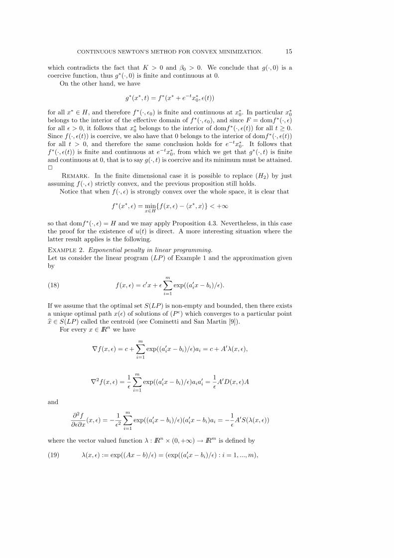
CONTINUOUS NEWTON’S METHOD FOR CONVEX MINIMIZATION. 15
which contradicts the fact that K > 0 and β0 > 0. We conclude that g(·, 0) is acoercive function, thus g∗(·, 0) is finite and continuous at 0.
On the other hand, we have
g∗(x∗, t) = f∗(x∗ + e−tx∗0, ε(t))
for all x∗ ∈ H, and therefore f∗(·, ε0) is finite and continuous at x∗0. In particular x∗0belongs to the interior of the effective domain of f∗(·, ε0), and since F = domf∗(·, ε)for all ε > 0, it follows that x∗0 belongs to the interior of domf∗(·, ε(t)) for all t ≥ 0.Since f(·, ε(t)) is coercive, we also have that 0 belongs to the interior of domf∗(·, ε(t))for all t > 0, and therefore the same conclusion holds for e−tx∗0. It follows thatf∗(·, ε(t)) is finite and continuous at e−tx∗0, from which we get that g∗(·, t) is finiteand continuous at 0, that is to say g(·, t) is coercive and its minimum must be attained.2
Remark. In the finite dimensional case it is possible to replace (H2) by justassuming f(·, ε) strictly convex, and the previous proposition still holds.
Notice that when f(·, ε) is strongly convex over the whole space, it is clear that
f∗(x∗, ε) = minx∈H
f(x, ε)− 〈x∗, x〉 < +∞
so that domf∗(·, ε) = H and we may apply Proposition 4.3. Nevertheless, in this casethe proof for the existence of u(t) is direct. A more interesting situation where thelatter result applies is the following.
Example 2. Exponential penalty in linear programming.Let us consider the linear program (LP ) of Example 1 and the approximation givenby
f(x, ε) = c′x + εm∑
i=1
exp((a′ix− bi)/ε).(18)
If we assume that the optimal set S(LP ) is non-empty and bounded, then there existsa unique optimal path x(ε) of solutions of (P ε) which converges to a particular pointx ∈ S(LP ) called the centroid (see Cominetti and San Martin [9]).
For every x ∈ IRn we have
∇f(x, ε) = c +m∑
i=1
exp((a′ix− bi)/ε)ai = c + A′λ(x, ε),
∇2f(x, ε) =1ε
m∑i=1
exp((a′ix− bi)/ε)aia′i =
1εA′D(x, ε)A
and
∂2f
∂ε∂x(x, ε) = − 1
ε2
m∑i=1
exp((a′ix− bi)/ε)(a′ix− bi)ai = −1εA′S(λ(x, ε))
where the vector valued function λ : IRn × (0,+∞) → IRm is defined by
λ(x, ε) := exp((Ax− b)/ε) = (exp((a′ix− bi)/ε) : i = 1, ...,m),(19)
16 F. ALVAREZ AND J.M. PEREZ
the diagonal matrix D(x, ε) := diag(λ(x, ε)) and S : IRm+ → IRm by
S(λ) := (λi lnλi : i = 1, ...,m),
with the convention 0 ln 0 = 0.For this approximation, we have Ω = domf(·, ε) = IRn and f(·, ε) is strongly
convex over bounded sets with parameter
βK(ε) =µK
εe−MK/ε
for suitable strictly positive constants µK and MK . Note that if the feasible set isunbounded, the exponential penalty function fails to be strongly convex with globalparameter (an analogous situation occurs for the log-barrier function) and we can notapply Theorem 4.1.
Proposition 4.4. Let ε : IR → IR+ be decreasing to 0 and consider the expo-nential penalty function f(·, ε) defined above. Then problem (P ε
t ) admits a uniquesolution trajectory u(t) which stays bounded as t → +∞.
Proof. In this case, f(·, ε) is strongly convex over bounded sets and it is notdifficult to prove that
domf∗(·, ε) = λ ∈ IRm : A′λ = −c, λ ≥ 0
which does not depend on ε. Hence, the existence and uniqueness of the optimaltrajectory u(t) follows from Proposition 4.3.
Let us consider once again the function
g(x, t) := f(x, ε(t))− e−t∇f(u0, ε0)′x.
Suppose that for a sequence tk → +∞ we have |u(tk)| → +∞. Passing to a subse-quence we can assume that u(tk)
|u(tk)| → z ∈ IRn for some z such that |z| = 1. Let x ∈ IRn
be fixed and such that Ax ≤ b. From the optimality of u(tk) and the definition of theexponential penalty we have
g(u(tk), tk) ≤ g(x, tk) ≤ c′x− e−tk∇f(u0, ε0)′x + ε(tk)m.(20)
Hence
c′u(tk)− e−tk∇f(u0, ε0)′u(tk) ≤ c′x− e−tk∇f(u0, ε0)′x + ε(tk)m,
and dividing by |u(tk)| and passing to the limit we get
c′z ≤ 0.
On the other hand, from (20) we also have
a′ixk − bi ≤ ε(tk) ln[(L + c′(x− u(tk))− e−tk∇f(u0, ε0)′(x− u(tk)) + ε(tk)m)/ε(tk)]
for a suitable constant L. From this it follows that a′iz ≤ 0 and we have found avector z 6= 0 such that c′z ≤ 0 and Az ≤ 0, which contradicts the boundedness of theoptimal set S(LP ). 2
With this result we have the existence of a bounded solution trajectory u(t) forthe associated dynamical system (ACN), and we obtain the estimate
|u(t)− x(ε(t))| ≤ |∇f(u0, ε0)|e−t
βK(ε(t))= Ce−t+M/ε(t)ε(t)(21)
CONTINUOUS NEWTON’S METHOD FOR CONVEX MINIMIZATION. 17
for suitable constants C > 0 and M > 0. If we have
limt→+∞
et−M/ε(t)
ε(t)= +∞
for all M > 0, then u(t) converges towards the centroid of S(LP ).Estimates like (21) may also be useful in order to obtain dual convergence results.
To be more precise we observe that by means of the Fenchel duality theory and inthe case of the exponential penalty approximation, it is possible to associate to thecorresponding problem (P ε) the following dual problem
(Dε) minb′λ + εm∑
i=1
λi(lnλi − 1) : A′λ = −c, λ ≥ 0
which can be interpreted as a penalized version of the classical dual problem of (LP ),namely
(D). minb′λ : A′λ = −c, λ ≥ 0
The previous dual was studied in [9] where it is shown that if x(ε) denotes the optimalsolution of the exponential penalized problem (P ε), then λ(x(ε), ε) (with λ(x, ε) de-fined as in (19)) is the unique optimal solution of (Dε). Moreover, λ(x(ε), ε) convergestowards a particular solution λ of the dual problem (D), characterized as the uniquesolution of
(D0) min∑i∈I0
λi(lnλi − 1) : A′λ = −c, λi = 0 i /∈ I0, λi ≥ 0 i ∈ I0.
where I0 = i : a′ix = bi for all x ∈ S(LP ).Denote for simplicity λ(x, t) := λ(x, ε(t)). Since
λi(u(t), t) = exp(a′i(u(t)− x(ε(t)))/ε(t)) exp((a′ix(ε(t))− bi)/ε(t))
= exp(a′i(u(t)− x(ε(t)))/ε(t))λi(x(ε(t)), t),
for all i = 1, ...,m, if we have
limt→+∞
|u(t)− x(ε(t))|ε(t)
= 0(22)
then
limt→+∞
λ(u(t), t) = limt→+∞
λ(x(ε(t)), t) = λ.
In order to have (22), using the estimate (21) we obtain
|u(t)− x(ε(t))|ε(t)
≤ |∇f(u0, ε0)|e−t
βK(ε(t))ε(t)= Ce−t+M/ε(t).
Therefore, we must have
limt→+∞
et−M/ε(t) = +∞
18 F. ALVAREZ AND J.M. PEREZ
or equivalently,
limt→+∞
t− M
ε(t)= +∞(23)
for all M > 0. For example, ε(t) = (1 + t)−α with 0 < α < 1.Finally, since (22) implies
limt→+∞
|u(t)− x(ε(t))| = 0,
we have the following result.Proposition 4.5. According to the previous definitions, if the parameter ε(t)
satisfies (23) then for every u0 ∈ IRn the unique solution of
(ACN)
[ 1ε(t)A
′D(u(t), ε(t))A]u(t)− ε(t)ε(t)A
′S(λ(u(t), t)) + A′λ(u(t), t) + c = 0u(0) = u0
converges as t → +∞ towards x the centroid of the optimal set S(LP ). Moreover
λ(u(t), t) = exp((Au(t)− b)/ε(t))
converges to λ a particular solution of the dual problem (D).Remark. In this case, the dual convergence for (ACN) comes from the sharp
estimate (21) for the distance between u(t) and the optimal trajectory x(ε(t)). Asimilar analysis for (DADA) trajectories may be involved since the correspondingestimate (6) is more complicated.
5. Epi-convergence and scaling. When the strong monotonicity parameterβ(ε) goes to 0, the increasing ill-conditioning of the Hessian operator of the approx-imating function represents an important problem from the numerical point of view.In this section, we shall see how in certain cases, an appropriate rescaling of the dif-ferential equation may be used to transform the original system into a renormalizedsystem where β(ε) is identically equal to 1.
In many situations (see [1, 17]) the epi-convergence and scaling method providesa variational characterization of the point x ∈ Argmin f obtained as a limit of theoptimal trajectory x(ε) := Argmin f(·, ε). In order to describe this method assumethat
f = epi− limε→0
f(·, ε),
that is, f is the Mosco-epi-limit of the parametric family of strongly convex functionsf(·, ε).
Let us define
h(x, ε) :=1
β(ε)[f(x, ε)−min f ]
and consider the rescaled minimization problem
(Rε) minh(x, ε) : x ∈ H
Note that (Rε) has also the point x(ε) as unique solution. Hence, with this rescal-ing no changes are introduced in the optimal trajectory, and the parametric family
CONTINUOUS NEWTON’S METHOD FOR CONVEX MINIMIZATION. 19
h(·, ε)ε>0 has the same regularizing properties as f(·, ε)ε>0 (coercivity, smooth-ness, etc.). However, for the new family of functions, the strong monotonicity propertyholds with parameter identically equal 1,
〈∂h(x, ε)− ∂h(y, ε), x− y〉 ≥ |x− y|2.
Suppose now that in addition to the epi-convergence of f(·, ε) we assume that h(·, ε)epi-converges towards a proper function h,
h = epi− limε→0
h(·, ε).
Then, as a consequence (see Attouch [1]) we have
〈∂h(x)− ∂h(y), x− y〉 ≥ |x− y|2,
so that h is a strongly convex function. Let x be its unique minimizer. Since h(x) =+∞ for x 6∈ Argmin f , then x ∈ Argmin f , and since from the Mosco-epi-convergencewe have that every limit point of the optimal path x(ε) : ε → 0 minimizes h, weconclude
limε→0
x(ε) = x.
Let us assume smoothness for the parametric family f(·, ε) in order to study thedynamical system
∇2f(u(t), ε(t))u(t) + ε(t)∂2f
∂ε∂x(u(t), ε(t)) +∇f(u(t), ε(t)) = 0.
If we re-scale this equation multiplying by 1/β(ε(t)) we get
∇2h(u(t), ε(t))u(t) +ε(t)
β(ε(t))∂2f
∂ε∂x(u(t), ε(t)) +∇h(u(t), ε(t)) = 0.
Assuming in addition that β(ε) is differentiable, we have
∂2f
∂ε∂x(x, ε) = β′(ε)∇h(x, ε) + β(ε)
∂2h
∂ε∂x(x, ε),
and therefore we get
∇2h(u(t), ε(t))u(t) + ε(t)∂2h
∂ε∂x(u(t), ε(t)) + [1 +
β′(ε(t)) · ε(t)β(ε(t))
]∇h(u(t), ε(t)) = 0.
Let us define
η(t) := t + ln(β(ε(t)))
and introduce the change of variables s = η(t). Denoting for simplicity v(s) :=u(η−1(s)) and h(x, s) := h(x, ε(η−1(s))) we get the equivalent differential equation
∇2h(v(s), s)v(s) +∂2h
∂s∂x(v(s), s) +∇h(v(s), s) = 0
where now the functions h(·, s) are strongly convex with a uniform parameter β = 1.
20 F. ALVAREZ AND J.M. PEREZ
For the asymptotic analysis it is natural to require that the reparametrizationsatisfies limt→+∞ η(t) = +∞. In the particular case above, this amounts to
limt→+∞
etβ(ε(t)) = +∞,
which is precisely the hypothesis made in Theorem 4.1. Under this condition, theestimate
|v(s)− x(ε(s))| ≤ e−s|∇h(v0, ε0)|
is equivalent to the one given in Theorem 4.1.
Example 3. Viscosity method.Let f be a closed convex function with optimal set Argmin f nonempty. Let theapproximation be
f(x, ε) = f(x) +ε
2|x|2 ,
which regularizes problem (P ) by adding a strongly convex term. In this case, wemay take β(ε) = ε. We have that
f = epi− limε→0
f(·, ε),
and if we define
h(x, ε) :=1ε[f(x, ε)−min f ] =
f(x)−min f
ε+|x|2
2,
then it is easy to prove that
h = epi− limε→0
h(·, ε)
where
h :=
12 |x|
2if x ∈ Argmin f
+∞ otherwise
Therefore, the unique solution x (ε) of (P ε) converges towards the element of minimalnorm in Argmin f (see Tikhonov and Arsenine [16]).
Assume that f ∈ C2(H; IR) and take the parameter function ε(t) = e−αt with0 < α < 1. Then
η(t) = t + ln(ε(t)) = (1− α)t
and the change of variables s = (1 − α)t leads to the function ε(s) = e−α
1−α s. If wechoose for instance α = 1
2 then
h(x, s) := es(f(x)−min f) +|x|2
2
and we obtainProposition 5.1. For every v0 ∈ H, the unique solution of
[es∇2f(v(s)) + I]v(s) + 2es∇f(v(s)) + v(s) = 0v(0) = v0
converges as s → +∞ towards x the element of minimal norm in Argmin f . 2
CONTINUOUS NEWTON’S METHOD FOR CONVEX MINIMIZATION. 21
ACKNOWLEDGMENT
We want to express our thanks to Prof. R. Cominetti for having suggested us thestudy of coupling approximating schemes with Newton’s method and for his valuablecomments and discussions.
REFERENCES
[1] Attouch H (1984) Variational convergence for functions and operators. Applicable Maths.Series, Pitman, London.
[2] Attouch H (1996) Viscosity solutions of minimization problems. SIAM J. Optimization,Vol. 6, No. 3 : 769-806
[3] Attouch H, Cominetti R (1996) A dynamical approach to convex minimization couplingapproximation with the steepest descent method. J. Diff. Equations 128 : 519-540.
[4] Aubin JP, Cellina A (1984) Differential Inclusions : Set-valued maps and viability theory.Springer-Verlag.
[5] Auslender A, Cominetti R, Haddou M. Asymptotic analysis for penalty methods inconvex and linear programming, to appear in Math. of Operations Research.
[6] Brezis H (1973) Operateurs maximaux monotones et semi-groups de contractions dansles espaces de Hilbert. Mathematical Studies 5, North-Holland, Amsterdam.
[7] Brezis H (1978) Asymptotic behavior of some evolution systems. Nonlinear EvolutionEquations, Academic Press.
[8] Bruck RE (1975) Asymptotic convergence of nonlinear contraction semi-groups in Hilbertspaces. J. Functional Analysis 18 : 15-26.
[9] Cominetti R, San Martın J. (1994) Asymptotic analysis of the exponential penalty tra-jectory in linear programming. Math. Programming. 67 : 169-187.
[10] Fiacco AV (1990) Perturbed variations of penalty function methods. Annals of Opera-tions Research 27 : 371-380.
[11] Furuya H, Miyashiba K, Kenmochi N (1986) Asymptotic behavior of solutions to a classof nonlinear evolution equations. J. Diff. Equations 62 : 73-94.
[12] Gonzaga CG (1992) Path-following methods for linear programming. SIAM Review 34: 167-224.
[13] Lemaire B (1993) An asymptotical variational principle associated with some differen-tial inclusions, continuous and discrete case. Conference colloque franco-vietnamien,ICAA, Hanoi.
[14] Megiddo N (1989) Pathways to the optimal set in linear programming. Progress in Math.Prog.: interior-point and related methods. Springer-Verlag 131-158.
[15] Rockafellar RT (1970) Convex Analysis. Princeton University Press, Princeton, N.J.[16] Tikhonov A, Arsenine V (1974) Methodes de resolution de problemes mal poses. MIR.[17] Torralba D (1996) Developpements asymptotiques pour les methodes d’approximation
par viscosite. CRAS, t. 322, Serie I : 123-128.


![MATH 614, Spring 2016 [3mm] Dynamical Systems …Dynamical Systems and Chaos Lecture 1: Examples of dynamical systems. A discrete dynamical system is simply a transformation f : X](https://img.pdfslide.net/doc/110x75/5fc3a613bb041d25ed5cc331/math-614-spring-2016-3mm-dynamical-systems-dynamical-systems-and-chaos-lecture.jpg)