Embed Size (px)
Citation preview
A Dynamical Systems Model forLanguage Change
Partha Niyogi*
Robert C. Berwick÷
Artificial Intelligence Laboratory,Center for Biological and Computational Learning,Massachusetts Institute of Technology,Cambridge, MA 02139
This paper formalizes linguists’ intuitions about language change, propos-ing a dynamical systems model for language change derived from a modelfor language acquisition. Linguists must explain not only how languagesare learned but also how and why they have evolved along certain trajec-tories and not others. While the language learning problem has focusedon the behavior of individuals and how they acquire a particular gram-mar from a class of grammars G, this paper considers a population ofsuch learners and investigates the emergent, global population character-istics of linguistic communities over several generations. It is argued thatlanguage change follows logically from specific assumptions about gram-matical theories and learning paradigms. Roughly, as the end productof two types of learning misconvergence over several generations, indi-vidual language learner behavior leads to emergent, population languagecommunity characteristics.
In particular, it is shown that any triple {G,A,P} of grammatical theory,learning algorithm, and initial sentence distributions can be transformedinto a dynamical system whose evolution depicts the evolving linguisticcomposition of a population. It is explicitly shown how this transforma-tion can be carried out for memoryless learning algorithms and param-eterized grammatical theories. As the simplest case, the example of twogrammars (languages) differing by exactly one binary parameter is formal-ized, and it is shown that even this situation leads directly to a quadratic(nonlinear) dynamical system, including regions with chaotic behavior.The computational model is applied to some actual data, namely the ob-served historical loss of “verb second” from old French to modern French.Thus, the formal model allows one to pose new questions about languagephenomena that one otherwise could not ask, such as the following.
1. Do languages (grammars) correctly follow observed historical tra-jectories? This is an evolutionary criteria for the adequacy of grammaticaltheories.
*Electronic mail address: [email protected].÷Electronic mail address: [email protected].
Complex Systems, 11 (1997) 161–204;” 1997 Complex Systems Publications, Inc.
162 P. Niyogi and R. C. Berwick
2. What are the logically possible dynamical change envelopes givena posited grammatical theory? These are rates and shapes of linguisticchange, including the possibilities for the past and the future.
3. What can be the effect of quantified variation in initial conditions?For example, population differences resulting from socio-political facts.
4. Other intrinsically interesting mathematical questions regarding lin-guistic dynamical systems.
1. Introduction: The paradox of language change
Much research on language has focused on how children acquire thegrammar of their parents from “impoverished” data presented to themduring childhood. The logical problem of language acquisition, cast for-mally, requires the learner to converge (attain) its correct target grammar(i.e., the language of its caretakers, that belongs to a class of possiblenatural language grammars). However, this learnability problem, ifsolved perfectly, would lead to a paradox: If generation after genera-tion children successfully attained the grammar of their parents, thenlanguages would never change with time. Yet languages do change.
Language scientists have long been occupied with describing phono-logical, syntactic, and semantic change, often appealing to an analogybetween language change and evolution, but rarely going beyond this.For instance, in [11] language change is talked about in this way:
Some general properties of language change are shared by otherdynamic systems in the natural world. . . In population biologyand linguistic change there is constant flux. . . . If one views alanguage as a totality, as historians often do, one sees a dynamicsystem.
Indeed, entire books have been devoted to the description of languagechange using the terminology of population biology: genetic drift, clines,and so forth. For a recent example, see Nichols (1992), Linguistic Diver-sity in Space and Time. Other scientists have explicitly made an appealto dynamical systems in this context; see especially Hawkins and Gell-Mann, 1989. Yet to the best of our knowledge, these intuitions havenot been formalized. That is the goal of this paper. A remarkable ef-fort in quantifying cultural change that has many potential unexploitedapplications to language is developed in [2].
In particular, we show formally that a model of language changeemerges as a logical consequence of language acquisition, an argumentmade informally by Lightfoot in [11]. We shall see that Lightfoot’s in-tuition that languages could behave just as though they were dynamicalsystems is essentially correct, as is his proposal for turning language ac-
Complex Systems, 11 (1997) 161–204

A Dynamical Systems Model for Language Change 163
quisition models into language change models. We can provide concreteexamples of both “gradual” and “sudden” syntactic changes, occurringover time periods of many generations to just a single generation. In[11] these sudden changes acting over a single generation are referredto as “catastrophic” but this term usually has a different meaning in thedynamical systems literature.
Many interesting points emerge from the formalization, some empir-ical, some programmatic.
1. Learnability is a well-known criterion for the adequacy of gram-matical theories. Our model provides an evolutionary criterion: Bycomparing the trajectories of dynamical linguistic systems to histori-cally observed trajectories, one can determine the adequacy of linguistictheories or learning algorithms.
2. We derive explicit dynamical systems corresponding to parame-trized linguistic theories (e.g., the head first/final parameter in head-driven phrase structure grammars or government-binding grammars)and memoryless language learning algorithms (e.g., gradient ascent inparameter space).
3. In the simplest possible case of a two-language (grammar) sys-tem differing by exactly one binary parameter, the system reduces to aquadratic map with the usual chaotic properties (dependent on initialconditions). That such complexity can arise even in the simplest casesuggests that formally modeling language change may be quite mathe-matically rich.
4. We illustrate the use of dynamical systems as a research tool byconsidering the loss of verb second position in old French as comparedto modern French. We demonstrate by computer modeling that onegrammatical parameterization advanced in the linguistics literature doesnot seem to permit this historical change, while another does.
5. We can more accurately model the time course of language change.In particular, in contrast to [10] and others, who mimic populationbiology models by imposing an S-shaped logistic change by assumption,we explain the time course of language change, and show that it neednot be S-shaped. Rather, language-change envelopes are derivable frommore fundamental properties of dynamical systems; sometimes they areS-shaped, but they can also be nonmonotonic.
6. We examine by simulation and traditional phase-space plots theform and stability of possible “diachronic envelopes” given varyingalternative language distributions, language acquisition algorithms, pa-rameterizations, input noise, and sentence distributions. The resultsbear on models of language “mixing,” so-called “wave” models forlanguage change, and other proposals in the diachronic literature.
Complex Systems, 11 (1997) 161–204

164 P. Niyogi and R. C. Berwick
7. As topics for future research, the dynamical system model pro-vides a novel possible source for explaining several linguistic changesincluding the evolution of modern Greek metrical stress assignment fromproto-Indo-European and Bickerton’s (1990) “creole hypothesis” con-cerning the striking fact that all creoles, irrespective of linguistic origin,have exactly the same grammar. In the latter case, the “universality” ofcreoles could be due to a parameterization corresponding to a commoncondensation point of a dynamical system, a possibility not consideredin Bickerton.
2. An acquisition-based model of language change
How does the combination of a grammatical theory and learning algo-rithm lead to a model of language change? We first note that just as withlanguage acquisition, there is a seeming paradox in language change: itis generally assumed that children acquire their caretaker (target) gram-mars without error. However, if this were always true, at first glancegrammatical changes within a population could seemingly never occur,since generation after generation children would successfully acquire thegrammar of their parents.
Of course, Lightfoot and others have pointed out the obvious solu-tion to this paradox: the possibility of slight misconvergence to targetgrammars could, over several generations, drive language change, muchas speciation occurs in the population biology sense [11]:
As somebody adopts a new parameter setting, say a new verb-object order, the output of that person’s grammar often differsfrom that of other people’s. This in turn affects the linguisticenvironment, which may then be more likely to trigger the newparameter setting in younger people. Thus a chain reaction maybe created.
We pursue this point in detail below. Similarly, just as in the biologicalcase, some of the most commonly observed changes in languages seemto occur as the result of the effects of surrounding populations, whosefeatures infiltrate the original language.
We begin our treatment by arguing that the problem of languageacquisition at the individual level leads logically to the problem of lan-guage change at the group or population level. Consider a populationspeaking a particular language. In our analysis this implies that allthe adult members of this population have internalized the same gram-mar (corresponding to the language they speak). This is the targetlanguage—children are exposed to primary linguistic data (PLD) fromthis source, typically in the form of sentences uttered by caretakers(adults). The logical problem of language acquisition is how childrenacquire this target language from their PLD, that is, to come up with
Complex Systems, 11 (1997) 161–204

A Dynamical Systems Model for Language Change 165
an adequate learning theory. We take a learning theory to be simply amapping from PLD to the class of grammars, usually effective, and soan algorithm. For example, in a typical inductive inference model, givena stream of sentences, an acquisition algorithm would simply update itsgrammatical hypothesis with each new sentence according to some pre-programmed procedure. An important criterion for learnability (Gold,1967) is to require that the algorithm converge to the target as the datagoes to infinity (identification in the limit).
Now suppose that we fix an adequate grammatical theory and anadequate acquisition algorithm. There are then essentially two meansby which the linguistic composition of the population could change overtime. First, if the PLD data presented to the child is altered (due to anynumber of causes, perhaps to presence of foreign speakers, contact withanother population, disfluencies, and the like), the sentences presentedto the learner (child) are no longer consistent with a single target gram-mar. In the face of this input, the learning algorithm might not convergeto the target grammar. Indeed, it might converge to some other gram-mar (g2); or it might converge to g2 with some probability, g3 with someother probability, and so forth. In either case, children attempting tosolve the acquisition problem using the same learning algorithm couldinternalize grammars different from the parental (target) grammar. Inthis way, in one generation the linguistic composition of the populationcan change. Sociological factors affecting language change affect lan-guage acquisition in exactly the same way, yet are abstracted away fromthe formalization of the logical problem of language acquisition. In thissame sense, we similarly abstract away such causes here, though theycan be brought into the picture as variation in probability distributionsand learning algorithms; we leave this open as a topic for additionalresearch.
Second, even if the PLD comes from a single target grammar, theactual data presented to the learner is truncated, or finite. After a finitesample sequence, children may, with nonzero probability, hypothesize agrammar different from that of their parents. This can again lead to adiffering linguistic composition in succeeding generations.
In short, the diachronic model is this: Individual children attemptto attain the target grammar of their caretakers. After a finite num-ber of examples, some are successful, but others may misconverge.The next generation will therefore no longer be linguistically homo-geneous. The third generation of children will hear sentences producedby the second—a different distribution—and they, in turn, will attaina different set of grammars. Over successive generations, the linguisticcomposition evolves as a dynamical system.
In this view, language change is a logical consequence of specificassumptions about the following.
Complex Systems, 11 (1997) 161–204

166 P. Niyogi and R. C. Berwick
1. The grammar hypothesis space—a particular parametrization, in a para-metric theory.
2. The language acquistion device—the learning algorithm the child uses todevelop hypotheses on the basis of data.
3. The primary linguistic data—the sentences presented to the children ofany one generation.
If we specify 1 through 3 for a particular generation, we should, inprinciple, be able to compute the linguistic composition for the nextgeneration. In this manner, we can compute the evolving linguisticcomposition of the population from generation to generation, that is, wearrive at a dynamical system. We now proceed to make this calculationprecise. We first review a standard language acquisition framework,and then show how to derive a dynamical system from it.
2.1 The language acquisition framework
To formalize the model, we must first state our assumptions aboutgrammatical theories, learning algorithms, and sentence distributions.
1. Denote by G a family of possible (target) grammars. Each grammar g Œ Gdefines a language L(g) Õ S* over some alphabet S in the usual way.
2. Denote by P a distribution on S* according to which sentences are drawnand presented to the learner. Note that if there is a well defined target gtand only positive examples from this target are presented to the learner,then P will have all its measure on L(gt), and zero measure on sentencesoutside. Suppose n examples are drawn in this fashion, one can then letDn = (S*)n be the set of all n-example data sets the learner might be pre-sented with. Thus, if the adult population is linguistically homogeneous(with grammar g1) then P = P1. If the adult population speaks 50 percentL(g1) and 50 percent L(g2) then P = 1/2P1 + 1/2P2.
3. Denote by A the acquisition algorithm that children use to hypothesizea grammar on the basis of input data. A can be regarded as a mappingfromDn to G. Acting on a particular presentation sequence dn ΠDn, thelearner posits a hypothesisA(dn) = hn ΠG. Allowing for the possibility ofrandomization, the learner could, in general, posit hi ΠGwith probabilitypi for such a presentation sequence dn.
The standard (stochastic version) learnability criterion (Gold, 1967) canthen be stated as follows.
For every target grammar gt ΠG with positive-only examples pre-sented according to P as above, the learner must converge to thetarget with probability 1, that is,
Prob[A(dn) = gt]ônÆ• 1.
Complex Systems, 11 (1997) 161–204
A Dynamical Systems Model for Language Change 167
One particular way of formulating the learning algorithm is as a localgradient ascent search through a space of target languages (grammars)defined by a one-dimensional n-length boolean array of parameters,with each distinct array fixing a particular grammar (language). With nparameters, there are 2n possible grammars (languages). For example,English and Japanese differ in that English is a so-called “verb first”language, while Japanese is “verb final.” Given this framework, wecan state the so-called triggering learning algorithm (TLA) from [5] asfollows.
Step 1. Initialize. Start at some random point in the (finite) space of possibleparameter settings, specifying a single hypothesized grammar with itsresulting extension as a language.
Step 2. Process input sentence. Receive a positive example sentence si at time ti(examples drawn from the language of a single target grammar L(Gt))from a uniform distribution on unembedded (nonrecursive) sentencesof the target language.
Step 3. Learnability on error detection. If the current grammar parses (gener-ates) si, then go to Step 2; otherwise, continue.
Step 4. Single-step hill climbing. Select a single parameter uniformly at random,to flip from its current setting, and change it (0 mapped to 1, 1 to 0)if and only if that change allows the current sentence to be analyzed;otherwise, leave the current parameter settings unchanged.
Step 5. Iterate. Go to Step 2.
Of course, this algorithm carries out “identification in the limit” inthe standard terminology of learning theory (Gold, 1967); it does nothalt in the conventional sense.
It turns out that if the learning algorithm A is memoryless (in thesense that previous example sentences are not stored) and G can bedescribed by a finite number of parameters, then we can describe thelearning system A, Gt, G as a Markov chain M with as many states asthere are grammars in G. More specifically the states in M are in one-to-one correspondence with grammars g ΠG and the target grammar Gtcorresponds to a particular target state st of M. The transition probabil-ities between states in M can be computed straightforwardly based onset difference calculations between the languages corresponding to theMarkov chain states. We omit the details of this demonstration here;for a simple, explicit calculation in the case of one parameter, see sec-tion 3. For a more detailed analysis of learnability issues for memorylessalgorithms in finite parameter spaces, consult [14, 18, 19].
2.2 From language learning to popuation dynamics
The framework for language learning has learners attempting to infergrammars on the basis of linguistic data. At any point in time n (i.e.,
Complex Systems, 11 (1997) 161–204

168 P. Niyogi and R. C. Berwick
after hearing n examples) the learner has a current hypothesis h withprobability pn(h). What happens when there is a population of learn-ers? Since an arbitrary learner has a probability pn(h) of developinghypothesis h (for every h ΠG), it follows that a fraction pn(h) of thepopulation of learners internalize the grammar h after n examples. Wetherefore have a current state of the population after n examples. Thisstate of the population might well be different from the state of theparent population. Assume for now that after n examples, maturationoccurs, that is, after n examples the learner retains the grammatical hy-pothesis for the rest of its life. Then one would arrive at the state of themature population for the next generation. This new generation nowproduces sentences for the following generation of learners accordingto the distribution of grammars in its population. Then, the processrepeats itself and the linguistic composition of the population evolvesfrom generation to generation.
We can now define a discrete time dynamical system by providing itstwo necessary components as follows.
1. A state space. A set of system states S. Here the state space is thespace of possible linguistic compositions of the population. Each state isdescribed by a distribution Ppop on G describing the language spoken bythe population. As usual, one needs to be able to define a s-algebra onthe space of grammars, and so on. This is unproblematic for the casesconsidered here because the set of grammars is finite. At any given pointin time t the system is in exactly one state s ΠS.
2. An update rule. How the system states change from one time step to thenext. Typically, this involves specifying a function f that maps st ΠS tost+1. In general, this mapping could be fairly complicated. For example,it could depend on previous states, future states, and so forth; for reasonsof space we do not consider all possibilities here. For more informationsee Strogatz, (1993).
For example, a typical linear dynamical system might consist of statevariables x (where x is a k-dimensional state vector) and a system of dif-ferential equations x¢ = Ax (A is a matrix operator) which characterizethe evolution of the states with time. RC circuits are a simple exampleof linear dynamical systems. The state (current) evolves as the capacitordischarges through the resistor. Population growth models (e.g., usinglogistic equations) provide other examples.
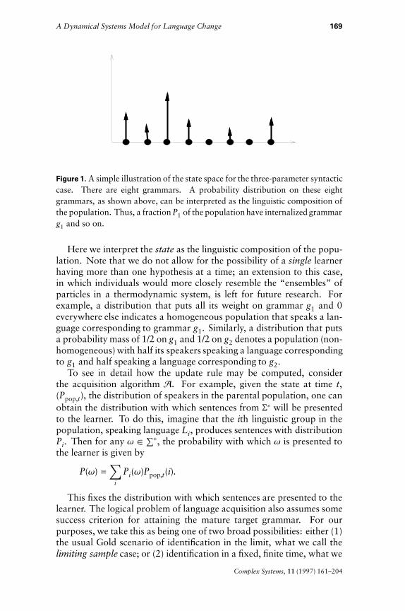
As a linguistic example, consider the three-parameter syntactic spacedescribed in [5]. This system defines eight possible “natural” grammars,that is, G has eight elements. We can picture a distribution on this spaceas shown in Figure 1. In this particular case, the state space is
S =ÏÔÔÌÔÔÓP Œ R8 |
8‚i=1
Pi = 1Ô̧Ô̋ÔÔ˛
.
Complex Systems, 11 (1997) 161–204
A Dynamical Systems Model for Language Change 169
Figure 1. A simple illustration of the state space for the three-parameter syntacticcase. There are eight grammars. A probability distribution on these eightgrammars, as shown above, can be interpreted as the linguistic composition ofthe population. Thus, a fraction P1 of the population have internalized grammarg1 and so on.
Here we interpret the state as the linguistic composition of the popu-lation. Note that we do not allow for the possibility of a single learnerhaving more than one hypothesis at a time; an extension to this case,in which individuals would more closely resemble the “ensembles” ofparticles in a thermodynamic system, is left for future research. Forexample, a distribution that puts all its weight on grammar g1 and 0everywhere else indicates a homogeneous population that speaks a lan-guage corresponding to grammar g1. Similarly, a distribution that putsa probability mass of 1/2 on g1 and 1/2 on g2 denotes a population (non-homogeneous) with half its speakers speaking a language correspondingto g1 and half speaking a language corresponding to g2.
To see in detail how the update rule may be computed, considerthe acquisition algorithm A. For example, given the state at time t,(Ppop,t), the distribution of speakers in the parental population, one canobtain the distribution with which sentences from S* will be presentedto the learner. To do this, imagine that the ith linguistic group in thepopulation, speaking language Li, produces sentences with distributionPi. Then for any w Œ ⁄*, the probability with which w is presented tothe learner is given by
P(w) =‚i
Pi(w)Ppop,t(i).
This fixes the distribution with which sentences are presented to thelearner. The logical problem of language acquisition also assumes somesuccess criterion for attaining the mature target grammar. For ourpurposes, we take this as being one of two broad possibilities: either (1)the usual Gold scenario of identification in the limit, what we call thelimiting sample case; or (2) identification in a fixed, finite time, what we
Complex Systems, 11 (1997) 161–204
170 P. Niyogi and R. C. Berwick
call the finite sample case. Of course, a variety of other success criteria,for example, convergence within some epsilon, or polynomial in the sizeof the target grammar, are possible; each leads to potentially differentlanguage change models. We do not pursue these alternatives here.
Consider case (2) first. Here, one draws n example sentences accord-ing to distribution P, and the acquisition algorithm develops hypotheses(A(dn) ΠG). One can, in principle, compute the probability with whichthe learner will posit hypothesis hi after n examples:
Finite Sample: Prob[A(dn) = hi] = pn(hi). (1)
The finite sample situation is always well defined, that is, the probabilitypn always exists. This is easy to see for deterministic algorithms, Adet.Such an algorithm would have a precise behavior for every data setof n examples drawn. In our case, the examples are drawn in i.i.d.fashion according to a distribution P on S*. It is clear that pn(hi) =P[{dn |Adet(dn) = hi}]. For randomized algorithms, the case is trickier,though tedious, but the probability still exists because all the finitechoice paths over all sequences of length n is enumerable. Previouswork [15–19] shows how to compute pn for randomized memorylessalgorithms.
Now turn to case (1), the limiting case. Here learnability requirespn(gt) to go to 1 for the unique target grammar gt if such a grammarexists. However, in general there need not be a unique target grammarsince the linguistic population can be nonhomogeneous. Even so, thefollowing limiting behavior might still exist:
Limiting Sample: limnƕ
Prob[A(dn) = hi] = p(hi). (2)
Turning from the individual child to the population, since the in-dividual child internalizes grammar hi Œ G with probability pn(hi) inthe “finite sample” case or with probability p(hi) “in the limit,” in apopulation of such individuals one would therefore expect a proportionpn(hi) or p(hi) respectively to have internalized grammar hi. In otherwords, the linguistic composition of the next generation is given byPpop,t+1(hi) = pn(hi) for the finite sample case and by Ppop,t+1(hi) = p(hi)in the limiting sample case. In this fashion,
Ppop,t ôA Ppop,t+1.
Remarks1. For a Gold-learnable family of languages and a limiting sample
assumption, homogeneous populations are always stable. This is simplybecause each child and therefore the entire population always eventuallyconverges to a single target grammar, generation after generation.
2. However, the finite sample case is different from the limiting samplecase. Suppose we have solved the maturation problem, that is, we know
Complex Systems, 11 (1997) 161–204

A Dynamical Systems Model for Language Change 171
roughly the time, or number of examples N the learner takes to developits mature (adult) hypothesis. In that case pN(h) is the probabilitythat a child internalizes the grammar h, and pN(h) is the percentage ofspeakers of Lh in the next generation. Note that under this finite sampleanalysis, even for a homogeneous population with all adults speakinga particular language (corresponding to grammar, g, say), pN(g) willnot be 1, that is, there will be a small percentage of learners who havemisconverged. This percentage could blow up over several generations,and we therefore have potentially unstable languages.
3. The formulation is very general. Any {A,G,P} triple yields a dy-namical system. Note that this probability could evolve with generationsas well, which would complete all the logical possibilites. However, forsimplicity, we assume that this does not happen. In short:
(G,A, {Pi})ô D(dynamical system).
4. The formulation also does not assume any particular linguistic the-ory, learning algorithm, or distribution with which sentences are drawn.Of course, we have implicitly assumed a learning model, that is, posi-tive examples are drawn in i.i.d. fashion and presented to the learner.Our dynamical systems formalization follows as a logical consequenceof this learning framework. One can conceivably imagine other learn-ing frameworks—these would potentially give rise to other kinds ofdynamical systems—but we do not formalize them here.
In previous works [15–19] we investigated the problem of learnabilitywithin parametric systems. In particular, we showed that the behaviorof any memoryless algorithm can be modeled as a Markov chain. Thisanalysis allows us to solve equations (1) and (2), and thus obtain theupdate equations for the associated dynamical system. Let us now showhow to derive such models in detail. We first provide the particularG,A, {Pi} triple, and then give the update rule.
The learning system tripleG: Assume there are n parameters, this leads to a space G with 2n different
grammars.
A: Let us imagine that the child learner follows some memoryless (incremen-tal) algorithm to set parameters. For the most part, we will assume thatthe algorithm is the TLA (the single step, gradient-ascent algorithm of[5]) or one of the variants discussed in [18, 19].
{Pi}: Let speakers of the ith language Li in the population produce sentencesaccording to the distribution Pi. For the most part we will assume in oursimulations that this distribution is uniform on degree-0 (unembedded)sentences, exactly as in the learnability analysis of [5] or [18, 19].
Complex Systems, 11 (1997) 161–204

172 P. Niyogi and R. C. Berwick
The update rule
We can now compute the update rule associated with this triple. Sup-pose the state of the parental population is Ppop,n on G. Then one canobtain the distribution P on the sentences of S* according to whichsentences will be presented to the learner. Once such a distribution isobtained, then given the Markov equivalence established earlier, we cancompute the transition matrix T according to which the learner updatesits hypotheses with each new sentence. From T one can finally computethe following quantities, one for the finite sample case and one for thelimiting sample case:
Prob[Learner’s hypothesis = hi Œ G after m examples]
= {12n (1, . . . , 1)¢Tm}[i].
Similary, making use of the limiting distributions of Markov chains(Resnick, 1992) one can obtain the following (where ONE is a 1/2n¥1/2n
matrix with all ones).
Prob[Learner’s hypothesis = hi“in the limit”]= (1, . . . , 1)¢(I - T +ONE)-1.
These expressions allow us to compute the linguistic composition of thepopulation from one generation to the next according to our analysis ofthe previous section.
RemarkThe limiting distribution case is more complex than the finite samplecase and requires some careful explanation. There are two possibilities.If there is just a single target grammar, then, by definition, the learnersall identify the target correctly in the limit, and there is no further changein the linguistic composition from generation to generation. This case isessentially uninteresting. If there are two or more target grammars, thenrecalling our analysis of learnability [18, 19], there can be no absorbingstates in the Markov chain corresponding to the parametric grammarfamily. In this situation, a single learner will oscillate between some setof states in the limit. In this sense, learners will not converge to anysingle, correct target grammar. However, there is a sense in which wecan characterize limiting behavior for learners: although a given learnerwill visit each of these states infinitely often in the limit, it will visit somemore often than others. The exact percentage the learner will be in aparticular state is given by equation (2). Therefore, since we know thefraction of the time the learner spends in each grammatical state in thelimit, we assume that this is the probability with which it internalizesthe grammar corresponding to that state in the Markov chain.
The following summarizes the basic computational framework formodeling language change.
Complex Systems, 11 (1997) 161–204

A Dynamical Systems Model for Language Change 173
1. Let p1 be the initial population mix, that is, the percentage of differ-ent language speakers in the community. Assuming that the ith groupof speakers produces sentences with probability Pi, we can obtain theprobability P with which sentences in S* occur for the next generation oflearners.
2. From P we can obtain the transition matrix T for the Markov learningmodel and the limiting distribution of the linguistic composition p2 forthe next generation.
3. The second generation now has a population mix of p2. We repeat step 1and obtain p3. Continuing in this fashion, in general we can obtain pi+1from pi.
This completes the abstract formulation of the dynamical systemmodel. Next, we choose three specific linguistic theories and learningparadigms to model particular kinds of language changes, with the goalof answering the following questions.
Can we really compute all the relevant quantities to specify the dynamicalsystem?
Can we evaluate the behavior (phase-space characteristics) of the resultingdynamical system?
Does the dynamical system model, the formalization, shed light on di-achronic models and linguistic theories generally?
In the remainder of this paper we give some concrete answers to thesequestions within the principles and parameters theory of modern linguis-tic theory. We turn first to the simplest possible mathematical case, thatof two languages (grammars) fixed by a single binary parameter. Wethen analyze a possibly more relevant, and more complex system, withthree binary parameters. Finally, to tackle a more realistic historicalproblem, we consider a five-parameter system that has actually beenused in other contexts to account for language change.
3. One-parameter models of language change
Consider the following simple scenario.
G: Assume that there are only two possible grammars (parameterized by oneboolean valued parameter) associated with two languages in the world,L1 and L2. (This might in fact be true in some limited linguistic contexts.)
P: Suppose that speakers who have internalized grammar g1 produce sen-tences with a probability distribution P1 (on the sentences of L1). Sim-ilarly, assume that speakers who have internalized grammar g2 produce
Complex Systems, 11 (1997) 161–204
174 P. Niyogi and R. C. Berwick
sentences with P2 (on sentences of L2).One can now define
a = P1[L1 » L2]; 1 - a = P1[L1 î L2]
and similarly
b = P2[L1 » L2]; 1 - b = P2[L2 î L1].
A: Assume that the learner uses a one-step, greedy, hill climbing approach tosetting target parameters. The TLA described earlier is one such example.
N: Let the learner receive just two example sentences before maturationoccurs, that is, after two example sentences, the current grammaticalhypothesis of the learner will be retained for the rest of its life.
Given this framework, the learnability question for this parametricsystem can be easily formulated and analyzed. Specifically, given aparticular target grammar (gi ΠG), and given example sentences drawnaccording to Pi and presented to the learnerA, one can ask whether thehypothesis of the learner will converge to the target.
Now it is possible to characterize the behavior of the individuallearner by a Markov chain with two states, one corresponding to eachgrammar (see section 2 and [18, 19]). With each example the learnermoves from state to state according to the transition probabilities of thechain. The transition probabilities can be calculated and depend uponthe distribution with which sentences are drawn and the relative overlapbetween the languages L1 and L2. In particular, if received sentencesfollow distribution P1, the transition matrix is T1. This would be thecase if the target grammar were g1. If the target grammar is g2 andsentences received according to distribution P2, the transition matrixwould be T2 as shown:
T1 = C 1 01 - a a G
T2 = C b 1 - b0 1 G .
Let us examine T1 in order to understand the behavior of the learnerwhen g1 is the target grammar. If the learner starts out in state 1(initial hypothesis g1), then it remains there forever. This is becauseevery sentence that it receives can be analyzed and the learner will neverhave to entertain an alternative hypothesis. Therefore the transition(1 Æ 1) has probability 1 and the transition (1 Æ 2) has probability 0.If the learner starts out in state 2, then after one example sentence, thelearner will remain there with probability a—the probability that thelearner will receive a sentence that it can analyze, that is, a sentence in
Complex Systems, 11 (1997) 161–204
A Dynamical Systems Model for Language Change 175
L1«L2. Correspondingly, with probability 1-a, the learner will receivea sentence that it cannot analyze and will have to change its hypothesis.Thus, the transition (2 Æ 2) has probability a and the transition (2 Æ 1)has probability 1 - a.
T1 characterizes the behavior of the learner after one example. Ingeneral, Tk
1 characterizes the behavior of the learner after k examples.It may be easily seen that as long as a < 1, the learner converges tothe grammar g1 in the limit irrespective of its starting state. Thus thegrammar g1 is Gold-learnable.
A similar analysis can be carried out for the case when the targetgrammar is g2. In this case, T2 describes the corresponding behavior ofthe learner, and g2 is Gold-learnable if b < 1. In short, the entire systemis Gold-learnable if a, b < 1, crucially assuming that maturation occursand the learner fixes a hypothesis forever after some N examples, withN given in advance. Clearly, if N is very large, then the learner will,with high probability, acquire the unique target grammar, whatever thatgrammar might be. At the same time, there is a finite probability thatthe learner will misconverge and this will have consequences for thelinguistic composition of the population as discussed in section 2. Forthe analysis that follows, we will assume that N = 2.
3.1 One-parameter systems: The linguistic population
Continuing with our one-parameter model, we next analyze distribu-tions over speakers. At any given point in time, the population consistsonly of speakers of L1 and L2. Consequently, the linguistic compositioncan be represented by a single variable, p: this will denote the fractionof the population speaking L1. Clearly 1 - p will speak L2. Thereforethis community of language composition over time can be explicitlycomputed as follows.
Theorem 1. The linguistic composition in the n+1th (pn+1) generationis provided by the following transformation on the linguistic composi-tion of nth generation (pn):
pn+1 = Ap2n + Bpn + C
where A = 1/2((1 - b)2 - (1 - a)2), B = b(1 - b) + (1 - a), and C = b2/2.
Proof. This is a simple specialization of the formula given in section 2.Details are left to the reader.
Remarks1. When a = b, the system has exponential growth. When a ! b
the dynamical system is a quadratic map (which can be reduced by atransformation of variables to the logistic, and shares the dynamicalproperties of the logistic). See Figure 2.
Complex Systems, 11 (1997) 161–204
176 P. Niyogi and R. C. Berwick
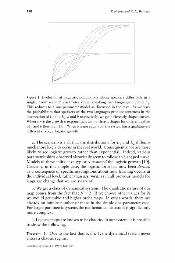
Figure 2. Evolution of linguistic populations whose speakers differ only in asingle, “verb second” parameter value, speaking two languages L1 and L2.This reduces to a one-parameter model as discussed in the text. As we varythe probabilities that speakers of the two languages produce sentences in theintersection of L1 and L2, a and b respectively, we get differently shaped curves.When a = b the growth is exponential, with different shapes for different valuesof a and b (less than 1.0). When a is not equal to b the system has a qualitativelydifferent shape, a logistic growth.
2. The scenario a ! b, that the distributions for L1 and L2 differ, ismuch more likely to occur in the real world. Consequently, we are morelikely to see logistic growth rather than exponential. Indeed, variousparametric shifts observed historically seem to follow an S-shaped curve.Models of these shifts have typically assumed the logistic growth [10].Crucially, in this simple case, the logistic form has now been derivedas a conseqence of specific assumptions about how learning occurs atthe individual level, rather than assumed, as in all previous models forlanguage change that we are aware of.
3. We get a class of dynamical systems. The quadratic nature of ourmap comes from the fact that N = 2. If we choose other values for Nwe would get cubic and higher order maps. In other words, there arealready an infinite number of maps in the simple one-parameter case.For larger parametric systems the mathematical situation is significantlymore complex.
4. Logistic maps are known to be chaotic. In our system, it is possibleto show the following.
Theorem 2. Due to the fact that a, b £ 1, the dynamical system neverenters a chaotic regime.
Complex Systems, 11 (1997) 161–204

A Dynamical Systems Model for Language Change 177
This observation naturally raises the question of whether nonchaoticbehavior holds for all grammatical dynamical systems, specifically thelinguistically “natural” cases. Or are there linguistic systems wherechaos will manifest itself? It would obviously be quite interesting ifall the natural grammatical spaces were nonchaotic. We leave these asopen questions.
We next turn to more linguistically plausible applications of the dy-namical systems model. We begin with a simple three-parameter systemas our first example, considering variations on the learning algorithm,sentence distributions, and sample size available for learning. We thenconsider a different, five-parameter system already presented in the lit-erature [3] as one intended to partially characterize the change from oldFrench to modern French.
4. A three-parameter system
In section 3 we developed the necessary mathematical and computa-tional tools to completely specify the dynamical systems correspondingto memoryless algorithms operating on finite parameter spaces. In thissection we investigate the behavior of these dynamical systems. Recallthat every choice of (G,A, {Pi}) gives rise to a unique dynamical system.We start by making specific choices for these three elements as follows.
G: This is a three-parameter syntactic subsystem described in [5]. Thus Ghas exactly eight grammars, generating languages from L1 through L8,as shown in the appendix of this paper (taken from [10]).
A: The memoryless algorithms we consider are the TLA, and variants bydropping either or both of the single-valued and greediness constraints.
{Pi}: For the most part, we assume sentences are produced according to auniform distribution on the degree-0 sentences of the relevant language,that is, Pi is uniform on (degree-0 sentences of) Li.
Ideally of course, a complete investigation of diachronic possibilitieswould involve varying G, A, and P and characterizing the resultingdynamical systems by their phase-space plots. Rather than explore thisentire space, we first consider only systems evolving from homogeneousinitial populations, under four basic variants of the learning algorithmA. This will give us an initial grasp of how linguistic populations canchange. Indeed, linguistic change has been studied before; even the dy-namical system metaphor itself has been invoked. Our computationalparadigm lets us say much more than these previous descriptions: Wecan say precisely what the rates of change will be and we can deter-mine what diachronic population curve changes will look like, withoutstipulating in advance that they must be S-shaped (sigmoid) or not, andwithout curve fitting to a predefined functional form.
Complex Systems, 11 (1997) 161–204

178 P. Niyogi and R. C. Berwick
4.1 Homogeneous initial populations
First we consider the case of a homogeneous population, that is, withoutnoise or confounding factors like foreign target languages. How stableare the languages in the three-parameter system in this case? To deter-mine this, we begin with a finite-sample analysis with n = 128 examplesentences (recall by the analysis of [15–19] that learners converge to tar-get languages in the three-parameter system with high probability afterhearing this many sentences). Some small proportion of the childrenmisconverge; the goal is to see whether this small proportion can drivelanguage change—and if so, in what direction. To give the reader someidea of the possible outcomes, let us consider the four possible variationsin the learning algorithm (±Single Step, ±Greedy) keeping the sentencedistributions and learning sample fixed.
4.1.1 Variation 1: A = TLA (+Single Step, +Greedy); Pi =Uniform;Finite Sample = 128
Suppose the learning algorithm is the TLA. Table 1 shows the languagemix after 30 generations. Languages are numbered from 1 to 8. Recallthat +V2 refers to a language that has the verb second property, and-V2 one that does not.
ObservationsSome striking patterns regarding the resulting population mixes can benoted.
1. All the +V2 languages are relatively stable, that is, the linguisticcomposition did not vary significantly over 30 generations. This meansthat every succeeding generation acquired the target parameter settingsand no parameter drifts were observed over time.
Initial Language Change to Language?(-V2) 1 2 (0.85), 6 (0.1)(+V2) 2 2 (0.98); stable(-V2) 3 6 (0.48), 8(0.38)(+V2) 4 4 (0.86); stable(-V2) 5 2 (0.97)(+V2) 6 6 (0.92); stable(-V2) 7 2 (0.54), 4(0.35)(+V2) 8 8 (0.97); stable
Table 1. Language change driven by misconvergence from a homogeneous initiallinguistic population. A finite-sample analysis was conducted allowing eachchild learner 128 examples to internalize its grammar. After 30 generations,initial populations drifted (or not, as shown in the table) to different finallinguistic compositions.
Complex Systems, 11 (1997) 161–204

A Dynamical Systems Model for Language Change 179
2. In contrast, populations speaking -V2 languages all drift to +V2languages. Thus a population speaking L1 winds up speaking mostlyL2 (85%). A population speaking language L7 gradually shifts to apopulation with 54 percent speaking L2 and 35 percent speaking L4(with a smattering of other speakers) and apparently remains basicallystable in this mix thereafter. Note that the relative stability of +V2languages and the tendency of -V2 languages to drift to +V2 is exactlycontrary to evidence in the linguistic literature. For example, in [11] itis claimed that the tendency to lose V2 dominates the reverse tendencyin languages of the world. Certainly, both English and French lost theV2 parameter setting, an empirically observed phenomenon that needsto be explained. Immediately then, we see that our dynamical systemdoes not evolve in the expected manner. The reason could be due to anyof the assumptions behind the model: the parameter space, the learningalgorithm, the initial conditions, or the distributional assumptions aboutsentences presented to learners. Exactly which is in error remains to beseen, but nonetheless our example shows concretely how assumptionsabout a grammatical theory and learning theory can make evolutionary,diachronic predictions—in this case, incorrect predictions that falsifythe assumptions.
• • • • • ••
•
•
•
•
•
••
• • • • • •
Figure 3. Percentage of a population speaking languages L1 and L2, measuredon the y-axis, as the population evolves over some number of generations,measured on the x-axis. The plot has been shown only up to 20 generations, asthe proportions of L1 and L2 speakers do not vary significantly thereafter. Notethat this curve is S-shaped. In [7] such a shape is imposed using models frompopulation biology, while we derive this shape as an emergent property of ourdynamical model. L1 and L2 differ only in the V2 parameter setting.
Complex Systems, 11 (1997) 161–204
180 P. Niyogi and R. C. Berwick
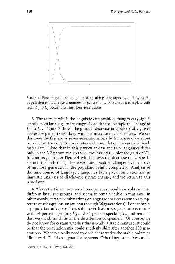
Figure 4. Percentage of the population speaking languages L5 and L2 as thepopulation evolves over a number of generations. Note that a complete shiftfrom L5 to L2 occurs after just four generations.
3. The rates at which the linguistic composition changes vary signif-icantly from language to language. Consider for example the change ofL1 to L2. Figure 3 shows the gradual decrease in speakers of L1 oversuccessive generations along with the increase in L2 speakers. We seethat over the first six or seven generations very little change occurs, butover the next six or seven generations the population changes at a muchfaster rate. Note that in this particular case the two languages differonly in the V2 parameter, so the curves essentially plot the gain of V2.In contrast, consider Figure 4 which shows the decrease of L5 speak-ers and the shift to L2. Here we note a sudden change: over a spaceof just four generations, the population shifts completely. Analysis ofthe time course of language change has been given some attention inlinguistic analyses of diachronic syntax change, and we return to thisissue later.
4. We see that in many cases a homogeneous population splits up intodifferent linguistic groups, and seems to remain stable in that mix. Inother words, certain combinations of language speakers seem to asymp-tote towards equilibrium (at least through 30 generations). For example,a population of L7 speakers shifts over five or six generations to onewith 54 percent speaking L2 and 35 percent speaking L4 and remainsthat way with no shifts in the distribution of speakers. Of course, wedo not know for certain whether this is really a stable mixture. It couldbe that the population mix could suddenly shift after another 100 gen-erations. What we really need to do is characterize the stable points or“limit cycles” of these dynamical systems. Other linguistic mixes can be
Complex Systems, 11 (1997) 161–204
A Dynamical Systems Model for Language Change 181
inherently unstable; they might drift systematically to stable situations,or might shift dramatically (as with language L1).
5. It seems that the observed instability and drifts are to a largeextent an artifact of the learning algorithm. Remember that the TLAsuffers from the problem of local maxima. We regard local maxima ofa language Li to be alternative absorbing states (sinks) in the Markovchain for that target language. This formulation differs slightly fromthe conception of local maxima in [5], a matter discussed at some lengthin [15]. Thus, according to our definition, L4 is not a local maxima forL5 and consequently no shift is observed. We note that those languageswhose acquisition is not impeded by local maxima (the +V2 languages)are stable over time. Languages that have local maxima are unstable; inparticular they drift to the local maxima over time. Now consider L7. Ifthis is the target language, then there are two local maxima (L2 and L4)and these are precisely the states to which the system drifts over time.The same is true for languages L5 and L3. In this respect, the behaviorof L1 is quite unusual since it actually does not have any local maxima,yet it tends to flip the V2 parameter over time.
Now let us consider a learning algorithm different from the TLAthat does not suffer from local maxima problems, to see whether thischanges the dynamical system results.
4.1.2 Variation 2: A = +Greedy, -Single Value; Pi = Uniform;Finite Sample = 128
Consider a simple variant of the TLA obtained by dropping the single-valued constraint. This implies that the learner is no longer constrainedto change just one parameter at a time: on being presented with asentence it cannot analyze, it chooses any of the alternative grammarsand attempts to analyze the sentence with it. Greediness is retained; thusthe learner retains its original hypothesis if the new one is also not able toanalyze the sentence. Given this new learning algorithm, and retainingall the other original assumptions, Table 2 shows the distribution ofspeakers after 30 generations.
ObservationsIn this situation there are no local maxima, and the evolutionary patterntakes on a very different nature. There are two distinct observations tobe made.
1. All homogeneous populations eventually drift to a strikingly simi-lar population mix, irrespective of what language they start from. Whatis unique about this mix? Is it a stable point (or attractor)? Furthersimulations and theoretical analyses are needed to resolve this question.
2. All homogeneous populations drift to a population mix of only+V2 languages. Thus, the V2 parameter is gradually set over succeed-
Complex Systems, 11 (1997) 161–204
182 P. Niyogi and R. C. Berwick
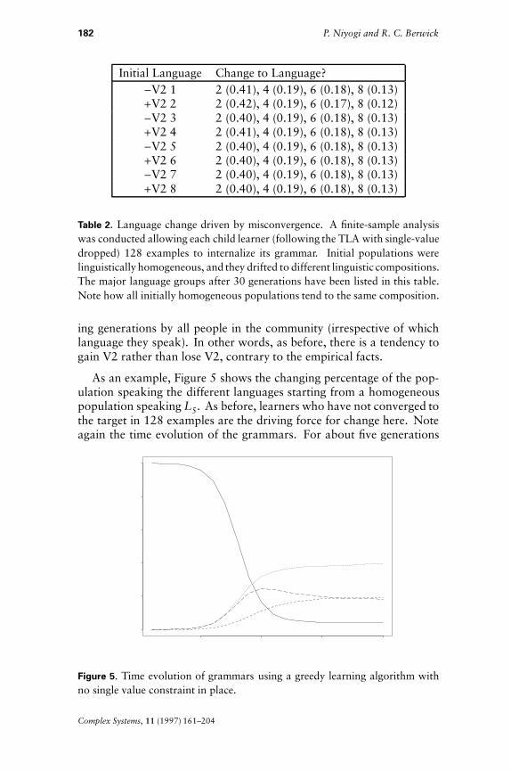
Initial Language Change to Language?-V2 1 2 (0.41), 4 (0.19), 6 (0.18), 8 (0.13)+V2 2 2 (0.42), 4 (0.19), 6 (0.17), 8 (0.12)-V2 3 2 (0.40), 4 (0.19), 6 (0.18), 8 (0.13)+V2 4 2 (0.41), 4 (0.19), 6 (0.18), 8 (0.13)-V2 5 2 (0.40), 4 (0.19), 6 (0.18), 8 (0.13)+V2 6 2 (0.40), 4 (0.19), 6 (0.18), 8 (0.13)-V2 7 2 (0.40), 4 (0.19), 6 (0.18), 8 (0.13)+V2 8 2 (0.40), 4 (0.19), 6 (0.18), 8 (0.13)
Table 2. Language change driven by misconvergence. A finite-sample analysiswas conducted allowing each child learner (following the TLA with single-valuedropped) 128 examples to internalize its grammar. Initial populations werelinguistically homogeneous, and they drifted to different linguistic compositions.The major language groups after 30 generations have been listed in this table.Note how all initially homogeneous populations tend to the same composition.
ing generations by all people in the community (irrespective of whichlanguage they speak). In other words, as before, there is a tendency togain V2 rather than lose V2, contrary to the empirical facts.
As an example, Figure 5 shows the changing percentage of the pop-ulation speaking the different languages starting from a homogeneouspopulation speaking L5. As before, learners who have not converged tothe target in 128 examples are the driving force for change here. Noteagain the time evolution of the grammars. For about five generations
Figure 5. Time evolution of grammars using a greedy learning algorithm withno single value constraint in place.
Complex Systems, 11 (1997) 161–204
A Dynamical Systems Model for Language Change 183
there is only a slight decrease in the percentage of speakers of L5. Thenthe linguistic patterns switch rapidly over the next seven generations toa relatively stable mix.
4.1.3 Variations 3 & 4: -Greedy, ±Single Value constraint; Pi = Uniform;Finite Sample = 128
Having dropped the single-value constraint, we consider the next ob-vious variation in the learning algorithm: dropping greediness whilevarying the single-value constraint. Again, our goal is to see whetherthis makes any difference in the resulting dynamical system. This givesrise to the following two different learning algorithms.
1. Allow the learning algorithm to pick any new grammar at most oneparameter value away from its current hypothesis (retaining the singlevalue constraint, but without greediness, i.e., the new grammar does nothave to be able to parse the current input sentence).
2. Allow the learning algorithm to pick any new grammar at each step (nomatter how far away from its current hypothesis).
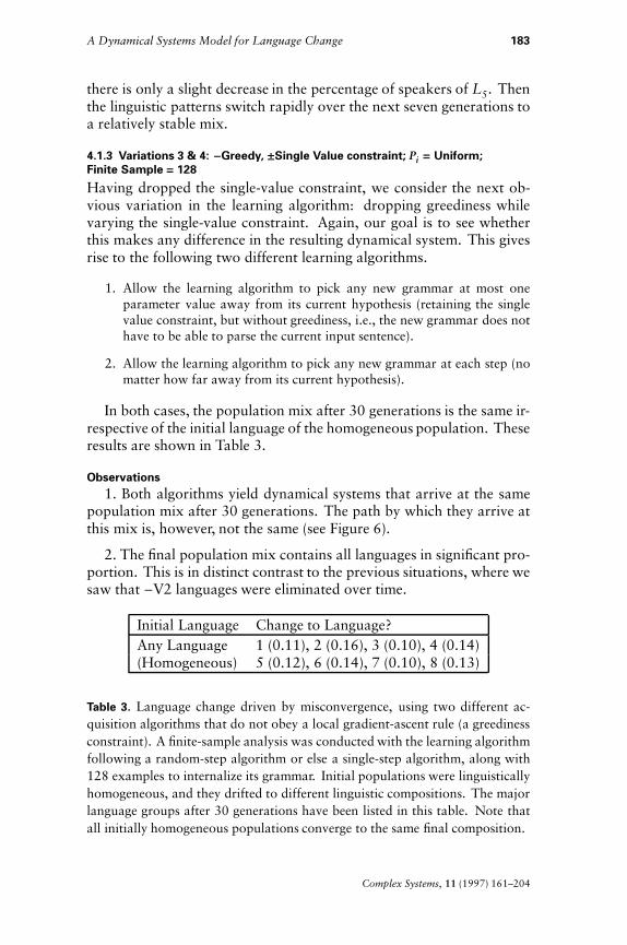
In both cases, the population mix after 30 generations is the same ir-respective of the initial language of the homogeneous population. Theseresults are shown in Table 3.
Observations1. Both algorithms yield dynamical systems that arrive at the same
population mix after 30 generations. The path by which they arrive atthis mix is, however, not the same (see Figure 6).
2. The final population mix contains all languages in significant pro-portion. This is in distinct contrast to the previous situations, where wesaw that -V2 languages were eliminated over time.
Initial Language Change to Language?Any Language 1 (0.11), 2 (0.16), 3 (0.10), 4 (0.14)(Homogeneous) 5 (0.12), 6 (0.14), 7 (0.10), 8 (0.13)
Table 3. Language change driven by misconvergence, using two different ac-quisition algorithms that do not obey a local gradient-ascent rule (a greedinessconstraint). A finite-sample analysis was conducted with the learning algorithmfollowing a random-step algorithm or else a single-step algorithm, along with128 examples to internalize its grammar. Initial populations were linguisticallyhomogeneous, and they drifted to different linguistic compositions. The majorlanguage groups after 30 generations have been listed in this table. Note thatall initially homogeneous populations converge to the same final composition.
Complex Systems, 11 (1997) 161–204

184 P. Niyogi and R. C. Berwick
Figure 6. Time evolution of linguistic composition for the situations wherethe learning algorithm is -Greedy, +Single Value constraint (dotted line), and-Greedy, -Single Value (solid line). Only the percentage of people speaking L1
(-V2) and L2 (+V2) are shown. The initial population is homogeneous andspeaks L1. The percentage of L1 speakers gradually decreases to about 11 per-cent. The percentage of L2 speakers rises to about 16 percent from 0 percent.The two dynamical systems converge to the same population mix; however,their trajectories are not the same—the rates of change are different, as shownin this plot.
4.2 Modeling diachronic trajectories
With a basic notion of how diachronic systems can evolve given differentlearning algorithms, we turn next to the question of population trajec-tories. While we can already see that some evolutionary trajectories havea “linguistically classical” S-shape, their smoothness can vary. However,our formalization allows us to say much more than this. Unlike theprevious work in diachronic linguistics that we are familiar with, we canexplore the space of possible trajectories, examining factors that affecttheir evolutionary time course, without assuming an a priori S-shape.
For example, in Bailey (1973) a “wave” model of linguistic change isproposed: linguistic replacements follow an S-shaped curve over time.In Bailey’s own words (from [10]):
A given change begins quite gradually; after reaching a certainpoint (say, twenty percent), it picks up momentum and proceedsat a much faster rate; and finally tails off slowly before reachingcompletion. The result is an S-curve: the statistical differencesamong isolects in the middle relative times of the change will begreater than the statistical differences among the early and lateisolects.
Complex Systems, 11 (1997) 161–204

A Dynamical Systems Model for Language Change 185
The idea that linguistic changes follow an S-curve has also beenproposed in [20, 22]. More specific logistic forms have been advancedin [4, 8, 9]. Here, the idea of a logistic functional form is borrowed frompopulation biology where it is demonstrable that the logistic governs thereplacement of organisms and of genetic alleles that differ in darwinianfitness. However, it is conceded in [9] that “unlike in the populationbiology case, no mechanism of change has been proposed from whichthe logistic form can be deduced.”
Crucially, in our case, we suggest a specific mechanism of change: anacquisition-based model where the combination of grammatical theory,learning algorithms, and distributional assumptions on sentences drivechange. The specific form might or might not be S-shaped, and mighthave varying rates of change. Of course, we do not mean to say that wecan simulate any possible trajectory—that would make the formalismempty. Rather, we are exploring the initial space of possible trajectories,given some example initial conditions that have been already advancedin the literature. Because the mathematics for dynamical systems is ingeneral quite complex, at present we cannot make general statementsof the form, “under these particular initial conditions the trajectory willbe sigmoidal, and under these other conditions it will not be.” Wehave conducted only very preliminary investigations demonstrating thatpotentially at least, reasonable, distinct initial conditions can lead todemonstrably different trajectories.
Among the other factors that affect evolutionary trajectories are mat-uration time, that is, the number of sentences available to the learnerbefore it internalizes its adult grammar, and the distributions with whichsentences are presented to the learner. We examine these in turn.
4.2.1 The effect of maturation time or sample size
One obvious factor influencing the evolutionary trajectories is the mat-urational time, that is, the number N of sentences the child is allowedto hear before forming its mature hypothesis. This was fixed at 128 inall the systems shown so far (based in part on our explicit computationfor the Markov convergence time in this situation). Figure 7 shows theeffect of varying N on the evolutionary trajectories. As usual, we plotonly a subspace of the population. In particular, we plot the percentageof L2 speakers in the population with each succeeding generation. Theinitial composition of the population was homogeneous (with peoplespeaking L1).
Observations1. The initial rate of change of the population is highest when the
maturation time is smallest, that is, the learner is allowed the leastamount of time to develop its mature hypothesis. This is not surprising.If the learner were allowed access to a lot of examples to make its mature
Complex Systems, 11 (1997) 161–204

186 P. Niyogi and R. C. Berwick
Figure 7. Time evolution of linguistic composition when varying maturation time(sample size). The learning algorithm used is the +Greedy, -Single Value. Onlythe percentage of people speaking L2 (+V2) is shown. The initial population ishomogeneous and speaks L1. The maturation time was varied through 8, 16,32, 64, 128, and 256, giving rise to the six curves shown. The curve with thehighest initial rate of change corresponds to eight examples for maturation time.The initial rate of change decreases as the maturation time N increases. Thevalue at which these curves asymptote also seems to vary with the maturationtime, and increases monotonically with it.
hypothesis, most learners would reach the target grammar. Very fewwould misconverge, and the linguistic composition would change littleover the next generation. On the other hand, if the learner were allowedvery few examples to develop its hypothesis, many would misconverge,possibly causing great change over one generation.
2. The “stable” linguistic compositions seem to depend upon matu-ration time. For example, if learners are allowed only eight examples,the percentage of L2 speakers rises quickly to about 0.26. On the otherhand, if learners are allowed 128 examples, the percentage of L2 speak-ers eventually rises to about 0.41.
3. Note that the trajectories do not have an S-shaped curve in contrastto the results in [9].
4. The maturation time is related to the order of the dynamical system.
4.2.2 The effect of sentence distributions (Pi)
Another important factor influencing evolutionary trajectories is thedistribution Pi with which sentences of the ith language Li are presentedto the learner. In a certain sense, the grammatical space and the learning
Complex Systems, 11 (1997) 161–204

A Dynamical Systems Model for Language Change 187
algorithm jointly determine the order of the dynamical system. On theother hand, sentence distributions are much like the parameters of thedynamical system (see section 4.3.2). Clearly the sentence distributionsaffect rates of convergence within one generation. Further, by puttinggreater weight on certain word forms rather than others, they mightinfluence systemic evolution in certain directions. While this is again anobvious point, the model lets us consider the alternatives precisely.
To illustrate the idea, consider as an example the interaction betweenL1 and L2 speakers in the community as the sentence distributionswith which these speakers produce sentences changes. Recall that sofar we have assumed that all speakers produce sentences with uniformdistributions on degree-0 sentences of their respective languages. Nowwe consider alternative distributions, parameterized by a value p asfollows.
1. Let L1,2 = L1 » L2.
2. P1: Speakers of L1 produce sentences so that all degree-0 sentences ofL1,2 are equally likely and their total probability is p. Further, sentencesof L1 î L1,2 are also equally likely, but their total proability is 1 - p.
3. P2: Speakers of L2 produce sentences so that all degree-0 sentences ofL1,2 are equally likely and their total probability is p. Further, sentencesof L2 î L1,2 are also equally likely, but their total proability is 1 - p.
4. Other Pi are all uniform over degree-0 sentences.
The parameter p determines the weight on the sentence patterns incommon between the languages L1 and L2. Figure 8 shows the evolutionof the L2 speakers as p varies. Here the learning algorithm is +Greedy,+Single Value (TLA, or local gradient ascent) and the initial populationis homogeneous, 100 percent L1 and zero percent L2. Note that thesystem moves in different ways as p varies. When p is very small (0.05),that is, sentences common to L1 and L2 occur infrequently, in the longrun the percentage of L2 speakers does not increase; the populationstays put with L1. However, as p grows, more strings of L2 occur,and the dynamical system changes so that the long-term percentageof L1 speakers decreases and that of L2 speakers increases. When preaches 0.75 the initial population evolves into a completely L2 speakingcommunity. After this, as p increases further, we notice that the L2speakers increase but can never rise to 100 percent of the population(see p = 0.95); there is still a residual L1 speaking component. This is tobe expected, because for such high values of p, many strings common toL1 and L2 occur frequently. This means that a learner could sometimesconverge to L1 just as well as L2, and some learners indeed begin to doso, increasing the number of the L1 speakers.
This example shows us that if we wanted a homogeneous L1 speak-ing population to move to a homogeneous L2 speaking population, by
Complex Systems, 11 (1997) 161–204

188 P. Niyogi and R. C. Berwick
Figure 8. The evolution of L2 speakers in the community for various values ofp (a parameter related to the sentence distributions Pi, see text). The algorithmused was the TLA, the initial population was homogeneous, speaking only L1.The curves for p = 0.05, 0.75, and 0.95 have been plotted as solid lines.
choosing our distributions appropriately, we could drive the grammat-ical dynamical system in the appropriate direction. It suggests anotherimportant application of the dynamical system approach: one can workbackwards, and examine the conditions needed to generate a changeof a certain kind. By checking whether such conditions could havepossibly existed historically, we can falsify a grammatical theory or alearning paradigm. Note that this example showed the effect of sentencedistributions, and how to alter them to obtain desired evolutionary en-velopes. One could, in principle, alter the grammatical theory or thelearning algorithm in the same fashion—leading to a tool to aid thesearch for an adequate linguistic theory. Again, we stress that we obvi-ously do not want so weak a theory that we can arrive at any possibleinitial conditions simply by carrying out reasonable changes to the sen-tence distributions. This may, of course, be possible; we have not yetexamined the general case.
4.3 Nonhomogeneous populations: Phase-space plots
For our three-parameter system we have been able to characterize theupdate rules for the dynamical systems corresponding to a variety oflearning algorithms. Each dynamical system has a specific update pro-cedure according to which the states evolve from some homogeneousinitial population. A more complete characterization of the dynamicalsystem would be achieved by obtaining phase-space plots of this sys-tem. Such phase-space plots are pictures of the state-space S filled with
Complex Systems, 11 (1997) 161–204
A Dynamical Systems Model for Language Change 189
trajectories obtained by letting the system evolve from various initialpoints (states) in the state space.
4.3.1 Phase-space plots: Grammatical trajectories
We described earlier the relationship between the state of the popu-lation in one generation and the next. In our case, let P denote aneight-dimensional vector variable (state variable). Specifically, P =(p1, . . . ,p8)¢ (with ⁄8
i=1 pi) as discussed before. The following schema re-iterates the chain of dependencies involved in the update rule governingsystem evolution. The state of the population at time t (in generations),allows us to compute the transition matrix T for the Markov chain asso-ciated with the memoryless learner. Now, depending upon whether wewant (1) an asymptotic analysis or (2) a finite sample analysis, we com-pute (1) the limiting behavior of Tm as m (the number of examples) goesto infinity (for an asymptotic analysis), or (2) the value of TN (where Nis the number of examples after which maturation occurs). This allowsus to compute the next state of the population. Thus P(t + 1) = g(P(t))where g is a complex nonlinear relation:
P(t)î P on S* î T î Tm îP(t + 1).
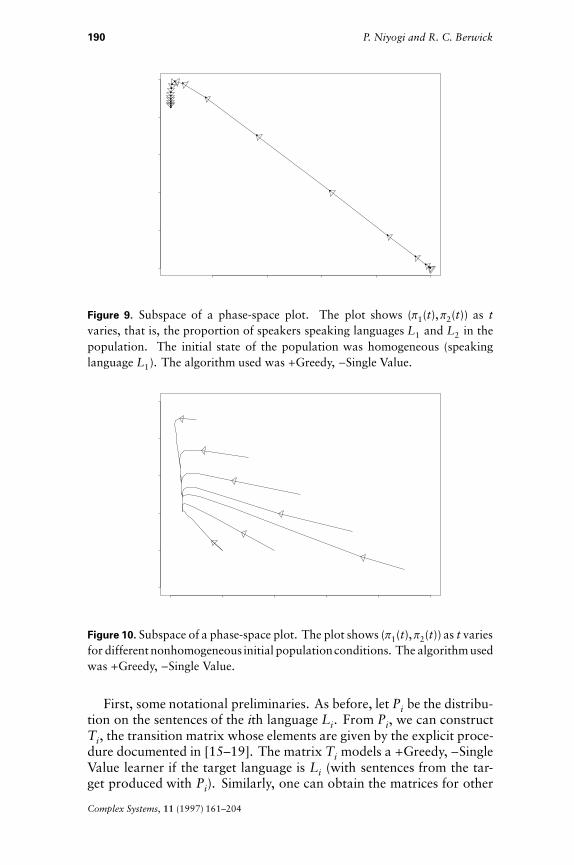
If we choose a certain initial condition P1, the system will evolve ac-cording to the above relation and one can obtain a trajectory of P inthe eight-dimensional space over time. Each initial condition yieldsa unique trajectory and one can then plot these trajectories obtain-ing a phase-space plot. Each such trajectory corresponds to a line inthe eight-dimensional plane given by ⁄8
i=1 pi = 1. One cannot directlydisplay such a high dimensional object, but we plot in Figure 9 the pro-jection of a particular trajectory onto a two-dimensional subspace givenby (p1(t),p2(t)) (the proportion of speakers of L1 and L2) at differentpoints in time.
As mentioned earlier, with a different initial condition we get a dif-ferent grammatical trajectory. The complete state-space picture is thusfilled with all the different trajectories corresponding to different initialconditions. Figure 10 shows this.
4.3.2 Stability issues
The phase-space plots show that many initial conditions yield trajec-tories that seem to converge to a single point in the state space. Inthe dynamical systems terminology, this corresponds to a fixed pointof the system—a population mix that stays at the same composition.Many natural questions arise at this stage. What are the conditions forstability? How many fixed points are there in a given system? Howcan we solve for them? These are interesting questions but detailedanswers are not within the scope of the current paper. In lieu of a morecomplete analysis we merely state here the equations that allow one tocharacterize the stable population mixes.
Complex Systems, 11 (1997) 161–204
190 P. Niyogi and R. C. Berwick
•••••
•
•
•
•
•••••••••••
Figure 9. Subspace of a phase-space plot. The plot shows (p1(t),p2(t)) as tvaries, that is, the proportion of speakers speaking languages L1 and L2 in thepopulation. The initial state of the population was homogeneous (speakinglanguage L1). The algorithm used was +Greedy, -Single Value.
Figure 10. Subspace of a phase-space plot. The plot shows (p1(t),p2(t)) as t variesfor different nonhomogeneous initial populationconditions. The algorithm usedwas +Greedy, -Single Value.
First, some notational preliminaries. As before, let Pi be the distribu-tion on the sentences of the ith language Li. From Pi, we can constructTi, the transition matrix whose elements are given by the explicit proce-dure documented in [15–19]. The matrix Ti models a +Greedy, -SingleValue learner if the target language is Li (with sentences from the tar-get produced with Pi). Similarly, one can obtain the matrices for other
Complex Systems, 11 (1997) 161–204
A Dynamical Systems Model for Language Change 191
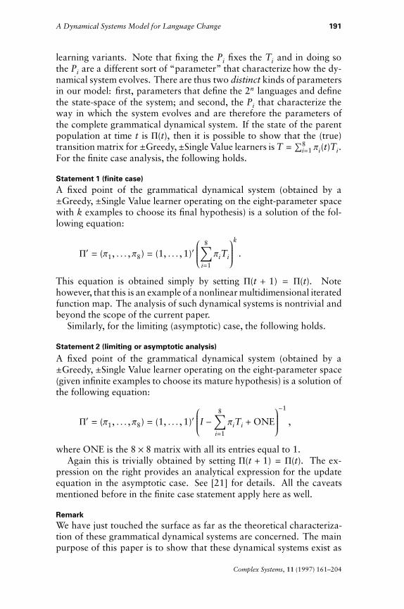
learning variants. Note that fixing the Pi fixes the Ti and in doing sothe Pi are a different sort of “parameter” that characterize how the dy-namical system evolves. There are thus two distinct kinds of parametersin our model: first, parameters that define the 2n languages and definethe state-space of the system; and second, the Pi that characterize theway in which the system evolves and are therefore the parameters ofthe complete grammatical dynamical system. If the state of the parentpopulation at time t is P(t), then it is possible to show that the (true)transition matrix for ±Greedy,±Single Value learners is T = ⁄8
i=1 pi(t)Ti.For the finite case analysis, the following holds.
Statement 1 (finite case)A fixed point of the grammatical dynamical system (obtained by a±Greedy, ±Single Value learner operating on the eight-parameter spacewith k examples to choose its final hypothesis) is a solution of the fol-lowing equation:
P¢ = (p1, . . . ,p8) = (1, . . . , 1)¢ÊÁÁÁÁÁË
8‚i=1
piTi
ˆ̃̃˜̃̃¯
k
.
This equation is obtained simply by setting P(t + 1) = P(t). Notehowever, that this is an example of a nonlinear multidimensional iteratedfunction map. The analysis of such dynamical systems is nontrivial andbeyond the scope of the current paper.
Similarly, for the limiting (asymptotic) case, the following holds.
Statement 2 (limiting or asymptotic analysis)
A fixed point of the grammatical dynamical system (obtained by a±Greedy, ±Single Value learner operating on the eight-parameter space(given infinite examples to choose its mature hypothesis) is a solution ofthe following equation:
P¢ = (p1, . . . ,p8) = (1, . . . , 1)¢ÊÁÁÁÁÁËI -
8‚i=1
piTi +ONEˆ̃̃˜̃̃¯
-1
,
where ONE is the 8 ¥ 8 matrix with all its entries equal to 1.Again this is trivially obtained by setting P(t + 1) = P(t). The ex-
pression on the right provides an analytical expression for the updateequation in the asymptotic case. See [21] for details. All the caveatsmentioned before in the finite case statement apply here as well.
RemarkWe have just touched the surface as far as the theoretical characteriza-tion of these grammatical dynamical systems are concerned. The mainpurpose of this paper is to show that these dynamical systems exist as
Complex Systems, 11 (1997) 161–204

192 P. Niyogi and R. C. Berwick
a logical consequence of assumptions about the grammatical space andan acquisition theory. We have exhibited only some preliminary sim-ulations with these systems. From a theoretical perspective, it wouldbe much more valuable to have complete characterizations of such sys-tems. In Strogatz (1993) it is suggested that nonlinear multidimensionalmappings with greater than three dimensions are likely to be chaotic. Itis also interesting to note that iterated function maps define fractal sets.Such investigations are beyond the scope of this paper, and might wellbe a fruitful area for further research.
5. From old French to modern French: An analysis revisited
So far, our examples have been based on a three-parameter linguistictheory for which we derived several different dynamical systems. Ourgoal was to concretely instantiate our philosophical arguments, sketch-ing the factors that influence evolutionary trajectories. In this section,we briefly consider a different parametric linguistic system studied in[3]. The historical context in which Clark and Roberts advanced theirlinguistic proposal is the evolution of modern French from old French.Their parameters are intended to capture some, but of course not all, ofthis change. They too use a learning algorithm—in their case, a geneticalgorithm—to account for historical change but do not analyze theirmodel from the dynamical systems viewpoint. Here we adopt their pa-rameterization, with all its strengths and weaknesses, but consider analternative learning paradigm and the dynamical systems approach.
Extensive simulations in section 4 reveal that while the learnabilityproblem of the three-parameter space can be solved by stochastic hillclimbing algorithms, the long-term evolution of these algorithms have abehavior that is at variance with the diachronic change actually observedin historical linguistics. In particular, we saw how there was a tendencyto gain rather than lose the V2 parameter setting. While this could wellbe an artifact of the class of learning algorithms considered, a morelikely explanation is that loss of V2 (observed in many languages of theworld such as French, English, and so forth) is due to an interaction ofparameters and triggers other than those considered in section 4. Weinvestigate this possibility and begin by first reviewing the alternativeparametric theory in [2].
5.1 The parametric subspace and data
We now consider a syntactic space involving five (boolean-valued) pa-rameters. We do not attempt to describe these parameters. The inter-ested reader should consult [3, 6] for details.
p1: Case assignment under agreement (p1 = 1) or not (p1 = 0).
p2: Case assignment under government (p2 = 1) or not (p2 = 0). Relevanttriggers for this parameter include “Adv V S” and “S V O.”
Complex Systems, 11 (1997) 161–204

A Dynamical Systems Model for Language Change 193
p3: Nominative clitics.
p4: Null Subject. Here relevant triggers would include “wh V S O.”
p5: Verb-second V2. Triggers include “Adv V S” and “S V O.”
These five parameters define a 32-grammar space. Each grammar inthis parametrized system can be represented by a string of five bits de-pending upon the values of p1, . . . , p5, for instance, the first bit positioncorresponds to case assignment under agreement. We can now look atthe surface strings (sentences) generated by each such grammar. For thepurpose of explaining how old French changed to modern French, thefollowing key sentences are considered in [2]. The parameter settingsrequired to generate each sentence are provided in brackets; an asteriskis a “does not matter” value and an “X” means any phrase.
The relevant dataadv V S [*1**1]SVO [*1**1] or [1***0]wh V S O [*1***]wh V S O [**1**]X (pro) V O [*1*11] or [1**10]X V s [**1*1]X s V [**1*0]X S V [1***0](S) V Y [*1*11]
The parameter settings provided in brackets set the grammars whichgenerate the sentence. For example, the sentence form “adv V S” (cor-responding to quickly ran John, an incorrect word order in English), isgenerated by all grammars that have case assignment under government(the second element of the array set to 1, p2 = 1) and verb second move-ment (p5 = 1). The other parameters can be set to any value. Clearlythere are eight different grammars that can generate (alternatively parse)this sentence. Similarly there are 16 grammars that generate the formS V O (eight corresponding to parameter settings of [*1**1] and eightcorresponding to parameter settings of [1***0]) and four grammarsthat generate (S) V Y.
RemarkNote that the sentence set considered in [2] is only a subset of thetotal number of degree-0 sentences generated by the 32 grammars inquestion. In order to directly compare their model with ours, we havenot attempted to expand the data set or fill out the space any further.As a result, all the grammars do not have unique extensional properties,that is, some generate the same set of sentences.
Complex Systems, 11 (1997) 161–204

194 P. Niyogi and R. C. Berwick
5.2 The case of diachronic syntax change in French
Continuing with the analysis from [2], within this parameter space, itis historically observed that the language spoken in France underwenta parametric change from the twelfth century to modern times. Inparticular, they point out that both V2 and prodrop are lost, illustratedby examples similar to the following.
Loss of null subjects: pro-drop
1. (old French; +pro drop)Si firent (pro) grant joie la nuit‘thus (they) made great joy the night’
2. (modern French; -pro drop)* Ainsi s’amusaient bien cette nuit‘thus (they) had fun that night’
Loss of V2
3. (old French; +V2)Lors oirent ils venir un escoiz de tonoire‘then they heard come a clap of thunder’
4. (modern French; -V2)* Puis entendirent-ils un coup de tonerre‘then they heard a clap of thunder’
In [2] it is observed that it has been argued this transition was broughtabout by the introduction of new word orders during the fifteenth andsixteenth centuries resulting in generations of children acquiring slightlydifferent grammars and eventually culminating in the grammar of mod-ern French. A brief reconstruction of the historical process (after [3])runs as follows.
Old French; setting [11011]
The language spoken in the twelfth and thirteenth centuries had verb-second movement and null subjects, both of which were dropped by thetwentieth century. The sentences generated by the parameter settingscorresponding to old French are the following.
Old Frenchadv V S - [*1**1]S V O - [*1**1] or [1***0]wh V S O [*1***]X (pro) V O [*1*11] or [1**10]
Note that from this data set it appears that both the case agreementand nominative clitics parameters remain ambiguous. In particular, old
Complex Systems, 11 (1997) 161–204

A Dynamical Systems Model for Language Change 195
French is in a subset-superset relation with another language (generatedby the parameter settings of 11111). In this case, possibly some kindof subset principle [1] could be used by the learner; otherwise it isnot clear how the data would allow the learner to converge to the oldFrench grammar in the first place. None of the ±Greedy, ±Single Valuealgorithms would converge uniquely to the grammar of old French.
The string (X)VS occurs with a frequency of 58 percent and SV(X)occurs with 34 percent in old French texts. It is argued that this fre-quency of (X)VS is high enough to cause the V2 parameter to trigger to+V2.
Middle FrenchIn middle French, the data is not consistent with any of the 32 targetgrammars (equivalent to a heterogenous population). Analysis of textsfrom that period reveal that some old forms (such as adv V S) decreasedin frequency and new forms (like adv S V) increased. It is argued in[3] that such a frequency shift causes “erosion” of V2, brings aboutparameter instability, and ultimately convergence to the grammar ofmodern French. In this transition period (i.e., when middle French wasspoken and written) the data is of the following form:
adv V S [*1**1]; SVO [*1**1] or [1***0]; wh V S O [*1***];wh V s O [**1**]; X (pro)V O [*1*11] or [1**10]; X V s [**1*1];X s V [**1*0]; X S V [1***0]; (s)VY [*1*11]
Thus, we have old sentence patterns like adv V S (though it decreasesin frequency and becomes only 10%), SVO, X (pro)V O, and wh V S O.The new sentence patterns which emerge at this stage are adv S V(increases in frequency to become 60%), X subjclitic V, V subjclitic(pro)V Y (null subjects), and wh V subjclitic O.
Modern French [10100]By the eighteenth century, French had lost both the V2 parameter settingas well as the null subject parameter setting. The sentence patternsconsistent with modern French parameter settings are SVO [*1**1]or [1***0], X S V [1***0], and V s O [**1**]. Note that this data,though consistent with modern French, will not trigger all the parametersettings. In this sense, modern French (just like old French) is notuniquely learnable from data. However, as before, we shall not concernourselves overly with this, for the relevant parameters (V2 and nullsubject) are uniquely set by the data here.
5.3 Some dynamical system simulations
We can obtain dynamical systems for this parametric space, for a TLA(or TLA-like) algorithm in a straightforward fashion. We show theresults of two simulations conducted with such dynamical systems.
Complex Systems, 11 (1997) 161–204
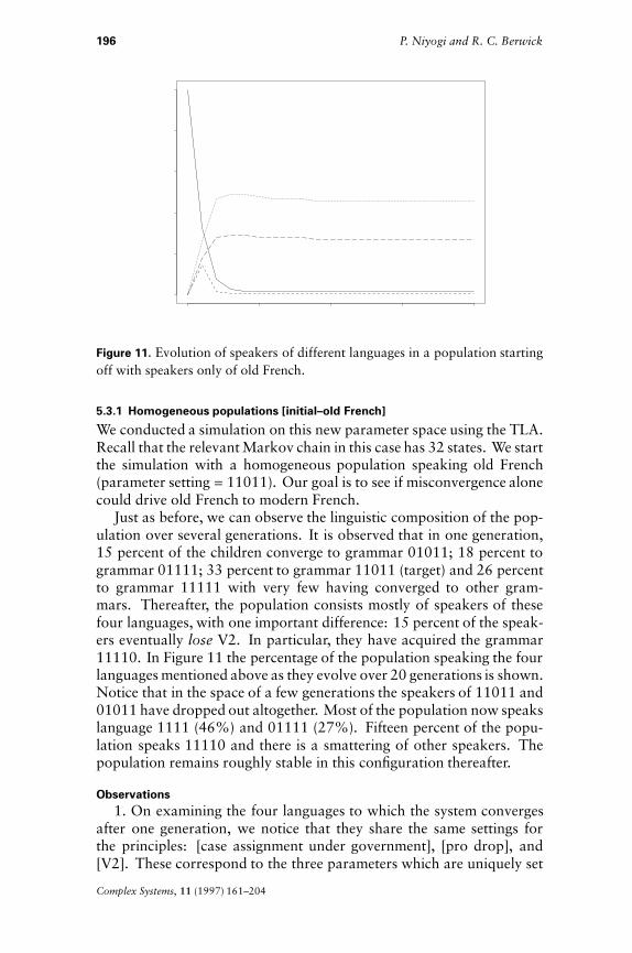
196 P. Niyogi and R. C. Berwick
Figure 11. Evolution of speakers of different languages in a population startingoff with speakers only of old French.
5.3.1 Homogeneous populations [initial–old French]
We conducted a simulation on this new parameter space using the TLA.Recall that the relevant Markov chain in this case has 32 states. We startthe simulation with a homogeneous population speaking old French(parameter setting = 11011). Our goal is to see if misconvergence alonecould drive old French to modern French.
Just as before, we can observe the linguistic composition of the pop-ulation over several generations. It is observed that in one generation,15 percent of the children converge to grammar 01011; 18 percent togrammar 01111; 33 percent to grammar 11011 (target) and 26 percentto grammar 11111 with very few having converged to other gram-mars. Thereafter, the population consists mostly of speakers of thesefour languages, with one important difference: 15 percent of the speak-ers eventually lose V2. In particular, they have acquired the grammar11110. In Figure 11 the percentage of the population speaking the fourlanguages mentioned above as they evolve over 20 generations is shown.Notice that in the space of a few generations the speakers of 11011 and01011 have dropped out altogether. Most of the population now speakslanguage 1111 (46%) and 01111 (27%). Fifteen percent of the popu-lation speaks 11110 and there is a smattering of other speakers. Thepopulation remains roughly stable in this configuration thereafter.
Observations1. On examining the four languages to which the system converges
after one generation, we notice that they share the same settings forthe principles: [case assignment under government], [pro drop], and[V2]. These correspond to the three parameters which are uniquely set
Complex Systems, 11 (1997) 161–204
A Dynamical Systems Model for Language Change 197
by data from old French. The other two parameters can take on anyvalue. Consequently, four languages are generated, all of which satisfythe data from old French.
2. Recall our earlier remark that, due to insufficient data, there wereequivalent grammars in the parameter system. It turns out that in thisparticular case, the grammars (01011) and (11011) are identical as far astheir extensional properties are concerned; as are the grammars (11111)and (01111).
3. There is subset relation between the two sets described in 2. Thegrammar (11011) is in a subset relation with (11111). This explainswhy after a few generations most of the population switches to either(11111) or (01111) (the superset grammars).
4. An interesting feature of the simulation is that 15 percent of thepopulation eventually acquires the grammar (11110), that is, they havelost the V2 parameter setting. This is the first sign of instability of V2that we have seen in our simulations so far (for greedy algorithms whichare psychologically preferred). Recall that for such algorithms, the V2parameter was very stable in our previous example.
5.3.2 Heterogenous populations (mixtures)
Section 5.3.1 showed that with no new (foreign) sentence patterns thegrammatical system starting out with only old French speakers showedsome tendency to lose V2. However, the grammatical trajectory did notterminate in modern French. In order to more closely duplicate this his-torically observed trajectory, we examine alternative initial conditions.We start our simulations with an initial condition which is a mixtureof two sources; data from old French and data from new French (re-producing in this sense, data similar to that obtained from the middleFrench period). Thus, children in the next generation observe new sur-face forms. Most of the surface forms observed in middle French arecovered by this mixture.
Observations1. On performing the simulations using the TLA as a learning al-
gorithm on this parameter space, an interesting pattern is observed.Suppose the learner is exposed to sentences with 90 percent generatedby old French grammar (11011) and 10 percent by modern Frenchgrammar (10100), within one generation 22 percent of the learnershave converged to the grammar (11110) and 78 percent to the grammar(11111). Thus, the learners set each of the parameter values to 1 exceptthe V2 parameter setting. Now, modern French is a nonV2 language;and 10 percent of data from modern French is sufficient to cause 22 per-cent of the speakers to lose V2. This is the behavior over one generation.
Complex Systems, 11 (1997) 161–204

198 P. Niyogi and R. C. Berwick
.
.
.
..
..
..
..
..
. . . . . .
...........
........
••
•
•
••
••
••
••
••
• • • • • •
Figure 12. Tendency to lose V2 as a result of new word orders introduced bymodern French source in our Markov model.
The new population (consisting of 78% speaking grammar (11111) and22% speaking grammar (11110)) remains stable forever.
2. Figure 12 shows the proportion of speakers who have lost V2after one generation as a function of the proportion of sentences fromthe modern French source. The shape of the curve is interesting. Forsmall values of the proportion of the modern French source the slope ofthe curve is greater than 1. Thus, there is a greater tendency of speakersto lose V2 than to retain it. This results in 10 percent of novel sentencesfrom the modern French source causing 20 percent of the population tolose V2; similarly 20 percent of novel sentences from the modern Frenchsource causes 40 percent of the speakers to lose V2. This effect wearsoff later. This seems to capture computationally the intuitive notion ofmany linguists that a small change in inputs provided to children coulddrive the system towards larger change.
3. Unfortunately, there are several shortcomings in this particularsimulation. First, we notice that mixing old and modern French sourcesdoes not cause the desired (historically observed) grammatical trajectoryfrom old to modern French (corresponding in our system to movementfrom state (11011) to state (10100) in our Markov chain). Althoughwe find that a small injection of sentences from modern French causesa larger percentage of the population to lose V2 and gain subject clitics(which are historically observed phenomena), nevertheless, the entirepopulation retains the null subject setting and case assignment undergovernment. It should be mentioned that it is argued in [3] that thechange in case assignment under government is the driving force which
Complex Systems, 11 (1997) 161–204

A Dynamical Systems Model for Language Change 199
allows alternate parse-trees to be formed and causes the parametric lossof V2 and null subject. In this sense, it is a more fundamental change.
4. If the dynamical system is allowed to evolve, it ends up in eitherof the two states (11111) or (11110). This is essentially due to thesubset relations these states (languages) have with other languages inthe system. Another complication in the system is the equivalence ofseveral different grammars (with respect to their surface extensions),for example, given the data we are considering, the grammars (01011)and (11011) (old French) generate the same sentences. This leads tomultiplicity of paths, convergence to more than one target grammar,and general inelegance of the state-space description.
Future DirectionsThere are several possibilities to consider here.
1. Using more data and filling out the state-space might yield greaterinsight. Note that studies in the development of other languages suchas Italian or Spanish within this framework might also be useful.
2. TLA-like hill climbing algorithms do not pay attention to the subsetprinciple explicitly. It would be interesting to explicitly program thisinto the learning algorithm and observe the evolution thereafter.
3. There are often cases when several different grammars generatethe same sentences or at least fit the data equally well. Algorithms thatlook only at surface strings are unable then to distinguish between themresulting in convergence to all of them with different probabilities inour stochastic setting. We showed an example of this for convergenceto four states earlier. An elegance criterion is suggested in [3] that looksat the parse-trees to decide between these grammars. This differencebetween strong generative capacity and weak generative capacity caneasily be incorporated into the Markov model as well. The transitionprobabilites, now, will not depend upon the surface properties of thegrammars alone, but also upon the elegance of derivation for eachsurface string.
4. Rather than the evolution of the population, one could look at theevolution of the distribution of words. One can also obtain bounds onfrequencies with which the new data in the middle French period mustoccur so that the correct drift is observed.
6. Conclusions and directions for future research
In this paper, we have argued that any combination of a grammaticaltheory and a learning paradigm leads to a model of grammatical evo-lution and diachronic change. A learning theory (paradigm) attempts
Complex Systems, 11 (1997) 161–204

200 P. Niyogi and R. C. Berwick
to account for how children (the individual child) solve the problem oflanguage acquisition. By considering a population of such “child learn-ers,” we have arrived at a model of the emergent, global, populationbehavior. The key point is that such a model is a logical consequence ofgrammatical and learning theories. Consequently, whenever a linguistsuggests a new grammatical, or learning theory, they are also suggestinga particular evolutionary theory—and the consequences of this need tobe examined.
6.1 Historical linguistics and diachronic criteria
From a programmatic persepective, this paper has two important conse-quences. First, it allows one to take a formal, analytic view of historicallinguistics. Most accounts of language change have tended to be de-scriptive in nature. In contrast, we place the study of historical ordiachronic linguistics in a formal framework. In this sense, our concep-tion of historical linguistics is closest in spirit to evolutionary theory andpopulation biology. Indeed, most previous attempts to model languagechange, such as [3, 10] have been influenced by the evolutionary models.
Second, this approach allows us to formally pose a diachronic cri-terion for the adequacy of grammatical theories. A significant body ofwork in learning theory has already sharpened the learnability criterionfor grammatical theories, in other words, the class of grammarsG mustbe learnable by some psychologically plausible algorithm from primarylinguistic data. Now we can go one step further. The class of grammarsG (along with a proposed learning algorithmA) can be reduced to a dy-namical system whose evolution must match that of the true evolutionof human languages (as reconstructed from historical data).
We have attempted to lay the framework for the development of re-search tools to study historical phenomena. To concretely demonstratethat the grammatical dynamical systems need not be impossibly diffi-cult to compute (or simulate), we explicitly showed how to transformparametrized theories, and memoryless learning algorithms to dynami-cal systems. The specific simulations of this paper are far too incompleteto have any long term linguistic implications, though, we hope, it cer-tainly forms a starting point for research in this direction. Nevertheless,certain interesting results were obtained.
1. It was shown that the V2 parameter was more stable in the three-parameter case than it was in the five-parameter case. This suggeststhat the loss of V2 (actually observed in history) might have more todo with the choice of parametrizations than learning algorithms, orprimary linguistic data (though we must suggest great caution beforedrawing strong conclusions on the basis of this study).
2. Some light was shed on the time course of evolution. In particular,it was shown how this was a derivative of more fundamental assump-
Complex Systems, 11 (1997) 161–204
A Dynamical Systems Model for Language Change 201
tions about initial population conditions, sentence distributions, andlearning algorithms.
3. Notions of system stability were formally developed. Thus, certainparameters could change with time, others might remain stable. Thiscan now be measured, and the conditions for stability or change can beinvestigated.
4. It was demonstrated that one could manipulate the system (bychanging the algorithm, sentence distributions, or maturational time)to allow evolution in certain directions. These logical possibilities sug-gest the kinds of changes needed in linguistics for greater explanatoryadequacy.
6.2 Further research
This has been our first attempt to define the boundaries of the languagechange problem as a dynamical system, there are several directions forfurther research.
1. From a linguistic perspective, one could examine alternative param-etrized theories, and track the change of certain languages in the contextof these theories (much like our attempt to track the change of Frenchin this paper). Some worthwhile attempts could include: (a) The studyof parametric stress systems [7]—and in particular, the evolution ofmodern Greek stress patterns from proto-Indo European. (b) The in-vestigation of the possibility that creoles correspond to fixed points inparametric dynamical systems, a possibility which might explain thestriking fact that all creoles (irrespective of the linguistic origin, i.e.,initial linguistic composition of the population) have the same gram-mar. (c) The evolution of modern Urdu, with Hindi syntax, and Persianvocabulary; a cross-comparison of so-called “phylogenetic” descriptivemethods currently used to trace back the development of an early, com-mon, proto-language.
2. From a mathematical perspective, one could take this research inmany directions including: (a) The formalization of the update rule forother grammatical theories and learning algorithms, and the characteri-zation of the dynamical systems implied. (b) A better characterization ofstability issues and phase-space plots. (c) The possibility of true chaoticbehavior—recall that our dynamical systems are multidimensional non-linear iterated function mappings.
It is our hope that research in this line will mature to make usefulcontributions, both to linguistics, and in view of the unusual nature ofthe dynamical systems involved, to the study of such systems from amathematical perspective.
Complex Systems, 11 (1997) 161–204

202 P. Niyogi and R. C. Berwick
Acknowledgments
This report describes research done at the Center for Biological andComputational Learning and the Artificial Intelligence Laboratory ofthe Massachusetts Institute of Technology. Support for the Center isprovided in part by a grant from the National Science Foundation undercontract ASC–9217041. R. C. Berwick was supported by a Vinton–Hayes Fellowship. P. Niyogi was supported by a grant from the NECCorporate Foundation.
Appendix
A. The three-parameter system of Gibson and Wexler
The three-parameter system discussed in [5] includes two parametersfrom X-bar theory. Specifically, they relate to specifier-head relations,and head-complement relations in phrase structure. The followingparametrized production rules denote this:
XP Æ SpecX¢(p1 = 0) or X¢Spec(p1 = 1)X¢ Æ CompX¢(p2 = 0) or X¢Comp(p2 = 1)X¢ Æ X.
A third parameter is related to verb movement. In German, andDutch root declarative clauses, it is observed that the verb occupiesexactly the second position. This verb-second phenomenon might ormight not be present in languages of the world, and this variation iscaptured by means of the V2 parameter.
Table 4 provides the unembedded (degree-0) sentences from each ofthe eight grammars (languages) obtained by setting the three parametersof section 4 to different values. The languages are referred to as L1through L8.
References
[1] R. C. Berwick, The Acquisition of Syntactic Knowledge (MIT Press, 1985).
[2] L. Cavalli-Sforza and M. Feldman, Cultural Transmission and Evolution:A Quantitative Approach (Princeton University Press, 1981).
[3] R. Clark and I. Roberts, “A Computational Model of Language Learn-ability and Language Change,” Linguistic Inquiry, 24(2) (1993) 299–345.
[4] G. Altmann et al., “A Law of Change in Language,” in Historical Linguis-tics, edited by B. Brainard (Studienverlag Dr. N. Brockmeyer., Bochum,FRG, 1982).
Complex Systems, 11 (1997) 161–204
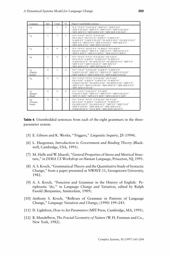
A Dynamical Systems Model for Language Change 203
Language Spec Comp V2 Degree-0 unembedded sentences
L1 1 1 0 “V S” “V O S” “V O1 O2 S” “AUX V S” “AUX V O S”“AUX V O1 O2 S” “ADV V S” “ADV V O S” “ADV V O1 O2 S”“ADV AUX V S” “ADV AUX V O S” “ADV AUX V O1 O2 S”
L2 1 1 1 “S V” “S V O” “O V S” “S V O1 O2”“O1 V O2 S” “O2 V O 1 S” “S AUX V” “S AUX V O”“O AUX V S” “S AUX V O1 O2” “O1 AUX V O2 S” “O2 AUX V O1 S”“ADV V S” “ADV V O S” “ADV V O1 O2 S” “ADV AUX V S”“ADV AUX V O S” “ADV AUX V O1 O2 S”
L3 1 0 0 “V S” “O V S” “O2 O1 V S” “V AUX S” “O V AUX S”“O2 O1 V AUX S” “ADV V S” “ADV O V S” “ADV O2 O1 V S”“ADV V AUX S” “ADV O V AUX S” “ADV O2 O1 V AUX S”
L4 1 0 1 “S V” “O V S” “S V O” “S V O2 O1” “O1 V O2 S”“O2 V O1 S” “S AUX V” “S AUX O V” “O AUX V S”“S AUX O2 O1 V” “O1 AUX O2 V S” “O2 AUX O1 V S” “ADV V S”“ADV V O S” “ADV V O2 O1 S” “ADV AUX V S”“ADV AUX O V S” “ADV AUX O2 O1 V S”
L5(English,French)
0 1 0 “S V” “S V O” “S V O1 O2” “S AUX V” “S AUX V O”“S AUX V O1 O2” “ADV S V” “ADV S V O” “ADV S V O1 O2”“ADV S AUX V” “ADV S AUX V O” “ADV S AUX V O1 O2”
L6 0 1 1 “S V” “S V O” “O V S” “S V O1 O2” “O1 V S O2”“O2 V S O1” “S AUX V” “S AUX V O” “O AUX S V”“S AUX V O1 O2” “O1 AUX S V O2” “O2 AUX S V O1” “ADV V S”“ADV V S O” “ADV V S O1 O2” “ADV AUX S V” “ADV AUX S V O”“ADV AUX S V O1 O2”
L7(Bengali,Hindi)
0 0 0 “S V” “S O V” “S O2 O1 V” “S V AUX”“S O2 O1 V AUX” “ADV S V” “ADV S O V” “ADV S O2 O1 V”“ADV S V AUX” “ADV S O V AUX” “ADV S O2 O1 V AUX”
L8(German,Dutch)
0 0 1 “S V” “S V O” “O V S” “S V O2 O1” “O1 V S O2”“O2 V S O1” “S AUX V” “S AUX O V” “O AUX S V”“O1 AUX S O2 V” “O2 AUX S O1 V” “ADV V S” “ADV V S O”“ADV V S O2 O1” “ADV AUX S V” “ADV AUX S O V”“S AUX O2 O1 V” “S O V AUX” “ADV AUX S O2 O1 V”
Table 4. Unembedded sentences from each of the eight grammars in the three-parameter system.
[5] E. Gibson and K. Wexler, “Triggers,” Linguistic Inquiry, 25 (1994).
[6] L. Haegeman, Introduction to Government and Binding Theory (Black-well, Cambridge, USA, 1991).
[7] M. Halle and W. Idsardi, “General Properties of Stress and Metrical Struc-ture,” in DIMA CS Workshop on Human Language, Princeton, NJ, 1991.
[8] A. S. Kroch, “Grammatical Theory and the QuantitativeStudy of SyntacticChange,” from a paper presented at NWAVE 11, Georgetown Universtiy,1982.
[9] A. S. Kroch, “Function and Grammar in the History of English: Pe-riphrastic ‘do,’" in Language Change and Variation, edited by RalphFasold (Benjamins, Amsterdam, 1989).
[10] Anthony S. Kroch, “Reflexes of Grammar in Patterns of LanguageChange,” Language Variation and Change, (1990) 199–243.
[11] D. Lightfoot, How to Set Parameters (MIT Press, Cambridge, MA, 1991).
[12] B. Mandelbrot, The Fractal Geometry of Nature (W. H. Freeman and Co.,New York, 1982).
Complex Systems, 11 (1997) 161–204

204 P. Niyogi and R. C. Berwick
[13] P. Niyogi, The Informational Complexity of Learning from Examples,PhD thesis, Massachussetts Institute of Technology, Cambridge, MA,1994.
[14] P. Niyogi, The Informational Complexity of Learning: Perspectives onNeural Networks and Generative Grammar (Kluwer Academic Publish-ers, Boston, 1997).
[15] P. Niyogi and R. C. Berwick, “Formalizing Triggers: A Learning Modelfor Finite Parameter Spaces,” Technical Report 1449, AI Laboratory, MIT,1993.
[16] P. Niyogi and R. C. Berwick, “A Markov Language Learning Model forFinite Parameter Spaces,” in Proceedings of 32nd Meeting of Associationfor Computational Linguistics, 1994.
[17] P. Niyogi and R. C. Berwick, “Formal Models for Learning Finite Pa-rameter Spaces,” Workshop on Cognitive Models of Language, TilburgUniversity, Ne., 1994. Also in Models of Language Learning: Inductiveand Deductive Approaches, edited by P. Broeder and J. Murre (MIT Press,Cambridge, MA, to appear).
[18] P. Niyogi and R. C. Berwick, “Learning from Triggers,” Linguistic Inquiry,27(4) (1996) 605–622.
[19] P. Niyogi and R. C. Berwick, “A Language Learning Model for FiniteParameter Spaces,” Cognition, 61 (1996) 161–193.
[20] C. Osgood and T. Sebeok, “Psycholinguistics: A Survey of Theory andResearch Problems,” Journal of Abnormal and Social Psychology, 49(4)(1954) 1–203.
[21] S. Resnick, Adventures in Stochastic Processes (Birkhauser, 1992).
[22] U. Weinreich, W. Labov, and M. I. Herzog, “Empirical Foundations for aTheory of Language Change,” in Directions for Historical Linguistics: ASymposium, edited by W. P. Lehmann (University of Texas Press, Austin,1968).
Complex Systems, 11 (1997) 161–204