Embed Size (px)
Citation preview

A Dynamically Bi-Orthogonal Method for Time-Dependent StochasticPartial Differential Equations II: Adaptivity and Generalizations
Mulin Chenga, Thomas Y. Houa,∗, Zhiwen Zhanga
aComputing and Mathematical Sciences, California Institute of Technology, Pasadena, CA 91125
Abstract
This is part II of our paper in which we propose and develop a dynamically bi-orthogonal method (DyBO)to study a class of time-dependent stochastic partial differential equations (SPDEs) whose solutions enjoya low-dimensional structure. In part I of our paper [9], we derived the DyBO formulation and proposednumerical algorithms based on this formulation. Some important theoretical results regarding consistencyand bi-orthogonality preservation were also established in the first part along with a range of numericalexamples to illustrate the effectiveness of the DyBO method. In this paper, we focus on the computationalcomplexity analysis and develop an effective adaptivity strategy to add or remove modes dynamically. Ourcomplexity analysis shows that the ratio of computational complexities between the DyBO method anda generalized polynomial chaos method (gPC) is roughly of order O((m/Np)
3) for a quadratic nonlinearSPDE, where m is the number of mode pairs used in the DyBO method and Np is the number of elementsin the polynomial basis in gPC. The effective dimensions of the stochastic solutions have been found tobe small in many applications, so we can expect m is much smaller than Np and computational savings ofour DyBO method against gPC are dramatic. The adaptive strategy plays an essential role for the DyBOmethod to be effective in solving some challenging problems. Another important contribution of this paperis the generalization of the DyBO formulation for a system of time-dependent SPDEs. Several numericalexamples are provided to demonstrate the effectiveness of our method, including the Navier-Stokes equationsand the Boussinesq approximation with Brownian forcing.
Keywords: Stochastic partial differential equations, Karhunen-Loeve expansion, Low-dimensionalstructure, Adaptivity algorithm, Sparsity, Stochastic flow
1. Introduction
This is the second part of the paper in developing a dynamically bi-orthogonal (DyBO) method forsolving time-dependent stochastic partial differential equations (SPDEs). It is well known that solvingSPDEs is very challenging due to the introduction of random variables and/or stochastic processes. Thecomputational cost increases exponentially fast as the number of random variables increases, which is alsoknown as the curse of dimensionality. In the past two decades, there has been tremendous progress innumerical simulations of the SPDEs. To our knowledge, these methods can be classified into two majorgroups, Monte Carlo methods [25, 26, 12, 2] and polynomial chaos methods [31, 5, 11, 32, 33, 20, 14].Monte Carlo methods are very robust and have the advantage of being independent of the dimensionalityof random variables, but they suffer from slow convergence due to their sampling nature. Polynomial chaosmethods provide more accurate approximations because of their spectral representation property. However,they suffer from the curse of dimensionality when the number of independent random variables is high.
∗Corresponding authorEmail addresses: [email protected] (Mulin Cheng), [email protected] (Thomas Y. Hou), [email protected]
(Zhiwen Zhang)
Preprint submitted to Elsevier January 11, 2013

Many of physical and engineering simulation problems that appear to be high-dimensional have somehidden low-dimensional or sparse structures. In recent years, we have witnessed a surge of interests inexploring sparse structures prevailing in many physical and engineering problems. These methods includecompressed sensing in signal reconstruction [6, 10], hierarchical matrix in discretization of integral operators[13], adaptive data analysis in signal processing [17, 18], signal processing for speech and music via l1
minimization [23, 34], proper orthogonal decomposition (POD) methods [3, 30], reduced basis (RB) methods[4, 24, 27] in solving parameterized PDEs, and the dynamically Orthogonal (DO) method in solving SPDEs[28, 29]. Most of these methods emphasize the use of spatial basis, but ignore stochastic basis. Thus theydo not preserve the bi-orthogonality of the spatial and the stochastic basis in their expansions.
The dynamically bi-orthogonal method (DyBO) that we proposed and developed in [9] and this paper(see also [8]) aims at preserving the dynamic bi-orthogonality, thus essentially tracking the Karhunen-Loeveexpansions [19, 21] of stochastic solutions. The Karhunen-Loeve expansion provides the optimal spatialand stochastic basis in the sense that it minimizes the total mean squared error and gives the sparsestrepresentation of stochastic solutions. One important advantage of DyBO over other reduced basis methodsis that we construct our reduced basis on the fly without the need to compute the reduced basis offline bysampling the stochastic solution. Another advantage of our method is that we do not need to compute thecovariance matrix, which could be very computationally expensive especially for high-dimensional problems.By solving an equivalent system that governs the evolution of the spatial and stochastic basis, our methodexplores the low-dimensional structure intrinsically hidden in a wide range of time-dependent SPDEs.
In part I of our paper [9], we introduced the derivation of dynamically bi-orthogonal formulation fortime-dependent SPDEs, and proved several theoretical properties, such as the dynamically bi-orthogonalitypreservation and the consistency between the DyBO formulation and the original SPDE. We also gave somedetails on the numerical implementation of the DyBO methods, including the representation of stochasticbasis and how to deal with eigenvalue crossing. One of the purposes of this paper is to study several impor-tant issues concerning the numerical performance of the DyBO method. These include the computationalcomplexity analysis and an adaptive strategy for adding or removing spatial and stochastic basis on the fly.We also generalize the dynamically bi-orthogonal formulation for a system of SPDEs and propose an effectiveparallel algorithm for DyBO. The parallel implementation is important for industrial-scale applications.
Our complexity analysis gives a detailed comparison between the complexity of our DyBO method andthat of gPC. Our analysis shows that the ratio between the complexity of DyBO and that of gPC is oforder O(m/Nd
h + (m/Np)3) for a quadratic nonlinear SPDE. Here m is the number of modes used in DyBO,
Np is the number of polynomial basis functions used in gPC, and Ndh is the total number of spatial grid
points in a d-dimensional problem. Typically, we expect m Np and m/Ndh (m/Np)
3. Thus the ratioof complexities between DyBO and gPC is roughly of order O((m/Np)
3). This has been confirmed by ournumerical experiments. Our complexity analysis also indicates that DyBO consumes less memory comparedwith gPC. The ratio of memory consumptions between DyBO and gPC is of order O(m/Np).
The ability to add or remove modes dynamically is crucial for the successful applications of our DyBOmethod to more challenging SPDEs. The adaptive strategy that we develop in this paper is based on solvingboth DyBO and gPC solutions with the same initial condition for a short time. We then extract the domi-nating spatial and stochastic modes by performing KL expansion on the difference of the two solutions. Byadding these dominant modes back to the DyBO formulation, we recapture previously unresolved dynamicsand maintain the accuracy of our method as these unresolved components become important later in time.We have applied this adaptive strategy to solve the 1D stochastic Burgers equation, the 2D incompressibleNavier-Stokes equation and the Boussinesq approximation with Brownian motion forcing. Our numericalresults indicate that the adaptive strategy indeed works quite effectively. The adaptive method gives the re-sults that are almost indistinguishable from those obtained by using a large m from the beginning. Further,we demonstrate the convergence of our method as the number of modes increases.
This paper is organized as follows. In Section 2, we provide a brief overview of the DyBO formulation.We perform the computational complexity analysis of our DyBO method in gPC version in Section 3, andcompare the complexity of DyBO with that of gPC. A parallel strategy is also proposed. In Section 4 alocal error analysis between DyBO method and gPC method is conducted and an adaptivity strategy inchanging the number of the spatial and stochastic basis is proposed. We generalize the DyBO formulation
2

for a system of time-dependent SPDEs in Section 5. Several numerical examples are provided in Section 6to demonstrate these ideas. Finally, some conclusion remarks will be made in Section 7.
2. Overview of the DyBO formulation for SPDEs
In order to set up notations for discussion and ease readers for further reading, we give a brief overviewof the DyBO formulation in this section. Further details can be found in part I of this paper [9]. Considerthe following time-dependent SPDE:
∂u
∂t(x, t, ω) = Lu(x, t, ω), x ∈ D ⊂ Rd, t ∈ [0, T ], ω ∈ Ω, (1a)
u(x, 0, ω) = u0(x, ω), x ∈ D, ω ∈ Ω, (1b)
B(u(x, t, ω)) = h(x, t, ω), x ∈ ∂D, ω ∈ Ω, (1c)
where L is a differential operator that may contain random coefficients and/or stochastic forces and B is alinear differential operator. The randomnesses may also enter the system through initial u0 and/or boundaryconditions B.
We assume the stochastic solution u(x, t, ω) of the system (1) is a second-order stochastic process at eachfixed time t > 0, i.e., u(·, t, ·) ∈ L2 (D × Ω). We consider the following truncated KL expansion,
u(x, t, ω) = u(x, t) +
m∑i=1
ui(x, t)Yi(ω, t) = u(x, t) + U(x, t)YT (ω, t) ≈ u(x, t, ω), (2)
where U = (u1, u2, · · · , um) and Y = (Y1, Y2, · · · , Ym). Define an anti-symmetrization operator Q : Rk×k →Rk×k and a partial anti-symmetrization operator Q : Rk×k → Rk×k as follows:
Q(A) =1
2
(A−AT
), Q(A) =
1
2
(A−AT
)+ diag(A),
where A ∈ Rk×k and diag(A) is a diagonal matrix whose diagonal entries are equal to those of matrix A.By enforcing the bi-orthogonal condition via Q and Q and a compatibility condition, we obtain the
DyBO formulation for the SPDE (1)
∂u
∂t= E [Lu] , (3a)
∂U
∂t= −UDT + E
[LuY
], (3b)
dY
dt= −YCT +
⟨Lu, U
⟩Λ−1
U , (3c)
where ΛU = diag(⟨UT , U
⟩) = (〈ui, uj〉 δij) ∈ Rm×m and Lu = Lu − E [Lu] and the m-by-m matrices C
and D can be solved uniquely from the following linear system,
C−Λ−1U Q (ΛUC) = 0, (4a)
D−Q (D) = 0, (4b)
DT + C = G∗(u,U,Y), (4c)
where the matrix G∗(u,U,Y) = Λ−1U
⟨UT , E
[LuY
]⟩∈ Rm×m.
The first two equations in the DyBO formulation (3) are time-dependent deterministic PDEs for the meansolution u and the spatial basis function U and they are coupled to the third equation, a system of stochasticODEs for the stochastic basis function Y. Various spatial discretization schemes, such as finite difference
3

schemes or spectral methods, along with ODE solvers, such as the fourth-order Runge-Kutta method canbe used to solve the first two deterministic PDEs. For the numerical simulations of the stochastic ODEs(3c), three representations of the stochastic modes Y have been proposed in the first part of the paper [9],leading to three variants of DyBO method, i.e., DyBO-MC, DyBO-gSC and DyBO-gPC. In this paper, weprimarily focus on DyBO-gPC methods, although similar arguments can also be applied to DyBO-MC andDyBO-gSC.
The Cameron-Martin theorem [5] implies the stochastic modes Yi(ω, t)’s in the KL expansion (2) can beapproximated by the linear combination of polynomial chaos, i.e.,
Yi(ω, t) =∑α∈J
Hα(ξ(ω))Aαi(t), i = 1, 2, · · · ,m, (5)
or in a matrix form, if we write H (ξ) = (Hα (ξ))α∈J as a row vector,
Y(ω, t) = H (ξ(ω)) A, (6)
where A ∈ RNp×m and Np is the number of polynomial basis functions. The expansion (2) now reads
u = u+ UATHT .
We can derive equations for u, U and A, instead of u, U and Y. In other words, the stochastic modes Yare identified with a matrix A ∈ RNp×m, which leads to the DyBO-gPC formulation of SPDE (1),
∂u
∂t= E [Lu] , (7a)
∂U
∂t= −UDT + E
[LuH
]A, (7b)
dA
dt= −ACT +
⟨E[HT Lu
], U⟩
Λ−1U , (7c)
where C(t) and D(t) can be solved from the linear system (4) with
G∗(u,U,Y) = Λ−1U
⟨UT , E
[LuY
]⟩= Λ−1
U
⟨UT , E
[LuH
]⟩A. (8)
By solving the system (7), we have an approximate solution to SPDE (1)
uDyBO-gPC = u+ UATHT .
The orthonormal property of Y implies that the columns of A are orthonormal, i.e., ATA = I ∈ Rm×m.We would like to point out that AAT ∈ RNp×Np in general is not an identity matrix as m Np if theSPDE solution has a low-dimensional or sparse structure.
3. Computational Complexity Analysis
As we discussed in the previous sections, the DyBO method explores the low-dimensional structure ofthe stochastic solutions of time-dependent SPDE and represents the solution in the most compact formin the L2 sense. The DyBO method not only offers savings in memory consumption, but also reduces thecomputational cost since we have much fewer entries to update in each step time compared to gPC methods.In this section, the storage complexity and the computational cost between the DyBO-gPC method and thegPC method will be analysed and compared. We provide the analysis for a typical scenario, i.e., the quadraticnonlinear PDE driven by stochastic forces. Examples of this type of SPDEs include the stochastic Burgersequation and the stochastic Naiver-Stokes equation. In Section 6, numerical examples will be provided toconfirm the complexity analysis.
4
To make the discussion concrete, we assume throughout this section that the randomness is given interms of r independent random variables ξi(ω) of the same distribution ρ(·), and the set of polynomial chaosbasis H has Np elements, i.e., the cardinality of multi-index set |J| = Np. Furthermore, Nh grid nodesare used along each direction of the hyper-cube D ∈ Rd, which results in a spatial grid of total Nd
h nodes.Such discretizations generally lead to large systems for both gSC and gPC. As a reminder, we have assumedthroughout this paper that the solutions of SPDEs under consideration enjoy low-dimensional structures,i.e., m Np.
3.1. Storage Complexity
Consider the gPC expansion of the stochastic solution, i.e.,
ugPC(x, t, ξ) = v(x, t) +∑α∈J
vα(x, t)Hα(ξ) = v(x, t) + V(x, t)HT (ξ), (9)
where V(x, t) = (vα(x, t))α∈J is a row vector of length Np. It is easy to derive the gPC formulation of theSPDE (1),
∂v
∂t= E [Lv] , (10a)
∂V
∂t= E
[LvH
]. (10b)
From the above gPC formulation (10), it is clear that v and V have to be updated in each time iteration.Thus, the storage cost of the gPC solution is proportional to O
(Ndh
)+ O
(NpN
dh
)= O
(NpN
dh
).
On the other hand, the mean u(x, t), the spatial modes U(x, t) = (u1(x, t), u2(x, t), · · · , um(x, t)) and thestochastic modes A(t) ∈ RNp×m in the DyBO-gPC formulation (7) are updated every time iteration, whichimplies the memory consumption is proportional to O
(Ndh
)+ O
(mNd
h
)+ O (mNp) = O
(mNd
h +mNp).
Here we have ignored the storage cost of axillary matrices in the DyBO formulation, i.e., matrices C, D andG∗ ∈ Rm×m, which are just O
(m2).
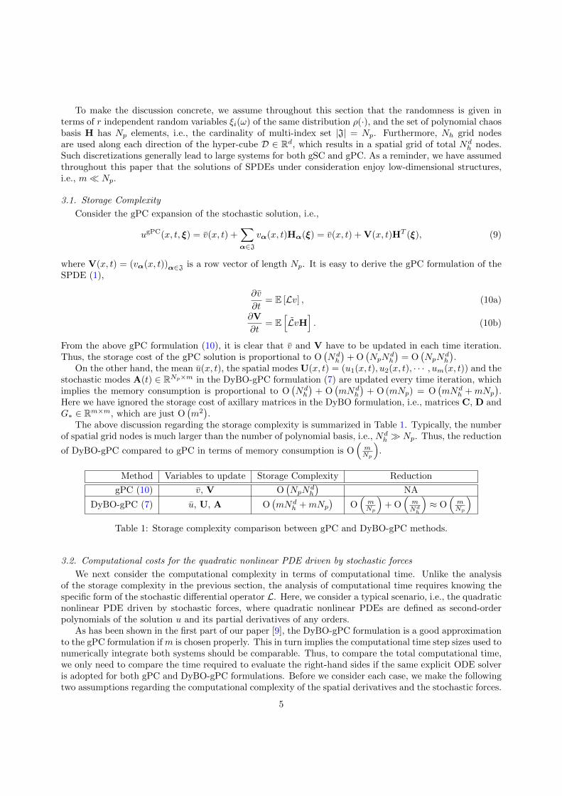
The above discussion regarding the storage complexity is summarized in Table 1. Typically, the numberof spatial grid nodes is much larger than the number of polynomial basis, i.e., Nd
h Np. Thus, the reduction
of DyBO-gPC compared to gPC in terms of memory consumption is O(mNp
).
Method Variables to update Storage Complexity Reduction
gPC (10) v, V O(NpN
dh
)NA
DyBO-gPC (7) u, U, A O(mNd
h +mNp)
O(mNp
)+ O
(mNdh
)≈ O
(mNp
)Table 1: Storage complexity comparison between gPC and DyBO-gPC methods.
3.2. Computational costs for the quadratic nonlinear PDE driven by stochastic forces
We next consider the computational complexity in terms of computational time. Unlike the analysisof the storage complexity in the previous section, the analysis of computational time requires knowing thespecific form of the stochastic differential operator L. Here, we consider a typical scenario, i.e., the quadraticnonlinear PDE driven by stochastic forces, where quadratic nonlinear PDEs are defined as second-orderpolynomials of the solution u and its partial derivatives of any orders.
As has been shown in the first part of our paper [9], the DyBO-gPC formulation is a good approximationto the gPC formulation if m is chosen properly. This in turn implies the computational time step sizes used tonumerically integrate both systems should be comparable. Thus, to compare the total computational time,we only need to compare the time required to evaluate the right-hand sides if the same explicit ODE solveris adopted for both gPC and DyBO-gPC formulations. Before we consider each case, we make the followingtwo assumptions regarding the computational complexity of the spatial derivatives and the stochastic forces.
5

Assumption 3.1. In our complexity analysis, we assume that the spatial derivative can be computed inlinear time and the gPC expansion of stochastic force F can be evaluated in linear time.
Under Assumption 3.1, any quadratic nonlinear PDE driven by stochastic forces is equivalent to thefollowing SPDE in regard to computational cost
∂u
∂t= Lu =
(Lu)2
+ f =(Lu)2
+ FHT , (11)
where L is a deterministic linear differential operator.We first consider the computational complexity of the gPC formulation (10) . With the gPC expansion
of the solution v = v + VHT , simple calculations give the gPC formulation for SPDE (11)
∂v
∂t=(Lv)2
+ LVLVT , (12a)
∂V
∂t= 2LvLV +
(LvαLvβT(H)
αβγ
)1×γ
+ F, (12b)
where the third-order tensor T(H) = (E [HαHβHγ ])αβγ . The computational cost of some typical terms
on the right hand sides of (12) is listed in Table 2. Note that the third-order tensor T(H) only depends
Term(Lv)2
LVLVT(LvαLvβT(H)
αβγ
)1×γ
F Total
Time O(Ndh
)O(NpN
dh
)O(N3pN
dh
)O(mNd
h
)O(N3pN
dh
)Table 2: The computational cost of the gPC formulation.
on the polynomial basis H and can be pre-computed, so its computational cost is ignored in this anal-
ysis. To evaluate a single entry of row vector(LvαLvβT(H)
αβγ
)1×γ
, we have to compute the summation∑α,β∈J LvαLvβT
(H)αβγ , which costs O
(N2pN
dh
), because a single evaluation of Lvα costs O
(Ndh
)and a total
of N2p terms are summed up. Therefore, the total cost of the whole row vector is O
(N3pN
dh
).
Next we consider the computational cost of DyBO-gPC. With the truncated KL expansion of the solutionu = u+ UATHT , simple calculations give the DyBO-gPC formulation for SPDE (11),
∂u
∂t=(Lu)2
+ LULUT , (13a)
∂U
∂t= −UDT + 2LuLU +
(LuiLujAαiAβjAγkT
(H)αβγ
)1×k︸ ︷︷ ︸
Term A
+FA, (13b)
∂A
∂t= −ACT + 2A
⟨LuLUT , U
⟩Λ−1U +
(T
(U)ijk AαiAβjT
(H)αβγ
)γ×k︸ ︷︷ ︸
Term B
+⟨FT , U
⟩Λ−1U , (13c)
where the third-order m-by-m-by-m tensor T(U) =(⟨LuiLuj , uk
⟩)ijk
, and matrices C and D can be solved
from the linear system (4) with
ΛUG∗ = 2⟨UT , LuLU
⟩+(T
(U)ijk AαiAβjAγlT
(H)αβγ
)k×l︸ ︷︷ ︸
Term C
+⟨UT , FA
⟩. (14)
Please note that the Einstein summation convention is implicitly assumed and the matrix-tensor product
should be computed in a recursive way, i.e., AαiAβjAγkT(H)αβγ = Aαi
(Aβj
(AγkT
(H)αβγ
)). It is not difficult
to find out such products can be computed in order of O(mN3
p
).
6

The computational costs of some typical terms on the right hand side of the DyBO-gPC formulation(13) are given in Table 3, where the estimate of term B goes as follows. The computation of T(U) in term
B costs O(m3Nd
h
), while the computation of the matrix-tensor product AαiAβjT
(H)αβγ costs O
(mN3
p
). The
last step of computing tensor-tensor product costs O(Npm
3). Thus, the total computational cost of term
B in Eq. (13c) is O(m3Nd
h
)+ O
(mN3
p
)+ O
(Npm
3)≤ O
(m3Nd
h
)+ O
(mN3
p
)since m Np.
Term LULUT⟨UT , LuLU
⟩T(U) Term A, B or C Total
Time mNdh m2Nd
h m3Ndh mN3
p +m3Ndh mN3
p +m3Ndh
Table 3: The computational costs of the DyBO-gPC formulation.
In light of the above discussions, the ratio of the computational costs between DyBO-gPC and gPC forthe quadratic nonlinear PDE driven by stochastic force is
O
(m
Ndh
)+ O
((m
Np
)3)≈ O
((m
Np
)3)
= O(mαN−βp
), (15)
where the exponents α = 3 and β = 3. In Section 6.2, we will numerically verify these two exponents forthe Navier Stokes equation driven by stochastic forces.
Remark 3.1. If the distribution of ξi’s is Gaussian, the tensor T(H) can be quite sparse, i.e., a few non-zeroentries out of total N3
p entries. However, this may not be the case for general distributions, so we do notexplore this sparsity in the above analysis. Later in numerical results, we will show that even if such sparsityis explored in numerical implementations of the gPC method, our DyBO-gPC method is still superior. Weshould also emphasize that gPC is a forward-model independent procedure while DyBO is derived from theforward model. In this sense, DyBO uses more information about the forward model than gPC.
3.3. Parallel computation strategy
Nowadays, parallelization almost becomes an indispensable tool for successful numerical simulations ofPDEs in industrial applications. Although the proposed DyBO methods have explored the inherent sparsitywithin SPDEs themselves, further computational reductions by parallelization are still necessary, especiallyfor spatially three-dimensional SPDEs with multiple physical components. Based on the computationalcomplexity analysis in the previous section, we propose a parallelization strategy based on domain decom-position for the quadratic nonlinear PDE driven by a stochastic force. Specifically, the computation costsof the third-order tensor TU, term A, B and C, dominate others and bear prohibitive costs of O
(m3Nd
h
).
Without resorting to other fancy parallelization techniques, the definitions of these terms actually suggesta simple strategy. We explain this in details for the computation of the third-order tensor T(U) while thesame strategy applies to other three terms similarly.
Suppose the whole spatial domain D is partitioned to Q disjoint subdomains Dq’s, i.e., ∪Qq=1Dq = D and
Dq1 ∩ Dq2 = ∅ for q1 6= q2. From the definition of T(U), each entry
T(U)ijk =
∫DLuiLujuk dx =
Q∑q=1
∫DqLuiLujuk dx =
Q∑q=1
T(U,q)ijk ,
where T(U,q) is the portion of T(U) on the q’th subdomain.Assume Q processors or computational nodes are available and the q’th processor is assigned to the
subdomain Dq . On the q’th processor, only the solutions constrained to the subdomain Dq, i.e., u|Diand U|Di , are stored in in-core memory. Thus, each process can compute its own portion of the third-
order tensor T(U,q) via Eq. (3.3). The result on each subdomain will be combined at the end to get T(U).The partition of domain may be problem-dependent. Numerical examples that confirm the speedup of theparallel computation strategy will be given in Section 6
7

4. Adaptive DyBO Algorithms
So far, we assume that the number of the spatial and stochastic basis pairs, ui, Yi’s, in the DyBOformulation is fixed to some integer m, which determines the number of functions U and the size of matrixA. Fixing m for all times is not a good strategy for practical applications. For example, some spatial andstochastic basis pairs may become negligibly small as the system evolves. Keeping such pairs in computationnot only wastes computational resource and increases computational time, but may also bring in unexpectednumerical instability since extremely small spatial modes may lead to ill-condition of the evolution system.On the other hand, some previously neglected mode pairs may become important later on. Ignoring themmay introduce O(1) numerical errors. Therefore, developing an adaptive strategy to add or remove modepairs dynamically is important for the success of DyBO method. In this section, we propose an adaptivestrategy to remove and add basis pairs on the fly for the DyBO-gPC formulation (7).
4.1. Type-KL error analysis
Our adaptive strategy is based on the analysis of a special type of error, which we call Type-KL errorand is defined as follows
ε = u− v, (16a)
ε = U−VA, (16b)
where v = v + VHT is the gPC solution defined in (10). Simple calculations give
∂ε
∂t= E [Lu− Lv] , (17a)
∂ε
∂t= E
[(Lu− Lv
)H]
A + εD + V(AAT − I
) ⟨E[LuHT
], U⟩
Λ−1U , (17b)
where Eq. (7b) (7c) and Eq. (4c) are used.
4.2. The adaptive algorithm
The strategy to remove modes is simple. Since the stochastic basis Y is orthonormal, i.e., E[Y 2i
]= 1,
we only need to check the norm of ui(x, t) to evaluate the importance of the mode pair (ui, Yi). At the end
of each time step, we compute λi = ‖ui‖2 and drop the ith pair ui, Yi if λi < ηλmax, where η ∈ (0, 1) is apre-selected threshold and λmax = maxi=1,2,··· ,m λi.
The situation to add mode pairs is more involved. Essentially, we want an algorithm to know when andwhat to add without sacrificing too much computational efficiency. A naive approach would be adding somespatial and stochastic mode pair if the smallest eigenvalue rises above some threshold, i.e., λmin > ηλmax.An immediate question is what spatial function and random variable should be used as the initial conditionsfor the new spatial mode um+1(x, t) and the stochastic mode Ham+1(t) with am+1(t) ∈ RNp×1 at sometime t = s. What’s more, the newly added mode pair may remain small and be removed later, which mayhappen repeatedly and should be avoided. In other words, we should estimate the growth rate of the largest
unresolved eigenvalue, i.e., dλm+1
dt ord√λm+1
dt and check if it may potentially grow above the threshold, i.e.,d√λm+1
dt ∆T ≥√ηλmax after some finite time interval ∆T . It turns out that these two questions are related.
The basis idea for adding mode pairs is to start from the same initial condition, evolve the SPDE systemby gPC and DyBO-gPC methods for a short time ∆s, respectively. We use the solution discrepancy at finaltime to estimate the growth rate of unresolved eigenvalues. If the growth rate is above certain threshold,we will use the dominant mode pair as the initial conditions for the new spatial and stochastic modes. Thisheuristic conjecture can be made more rigorous by looking at the type-KL errors that we discussed in theprevious subsection.
Suppose at time t = s, the DyBO-gPC solution
u(x, s, ξ) = u(x, s) + U(x, s)A(s)TH(ξ)T (18)
8
remains a good approximation to the gPC solution, i.e.,
v(x, s, ξ) ≈ u(x, s, ξ). (19)
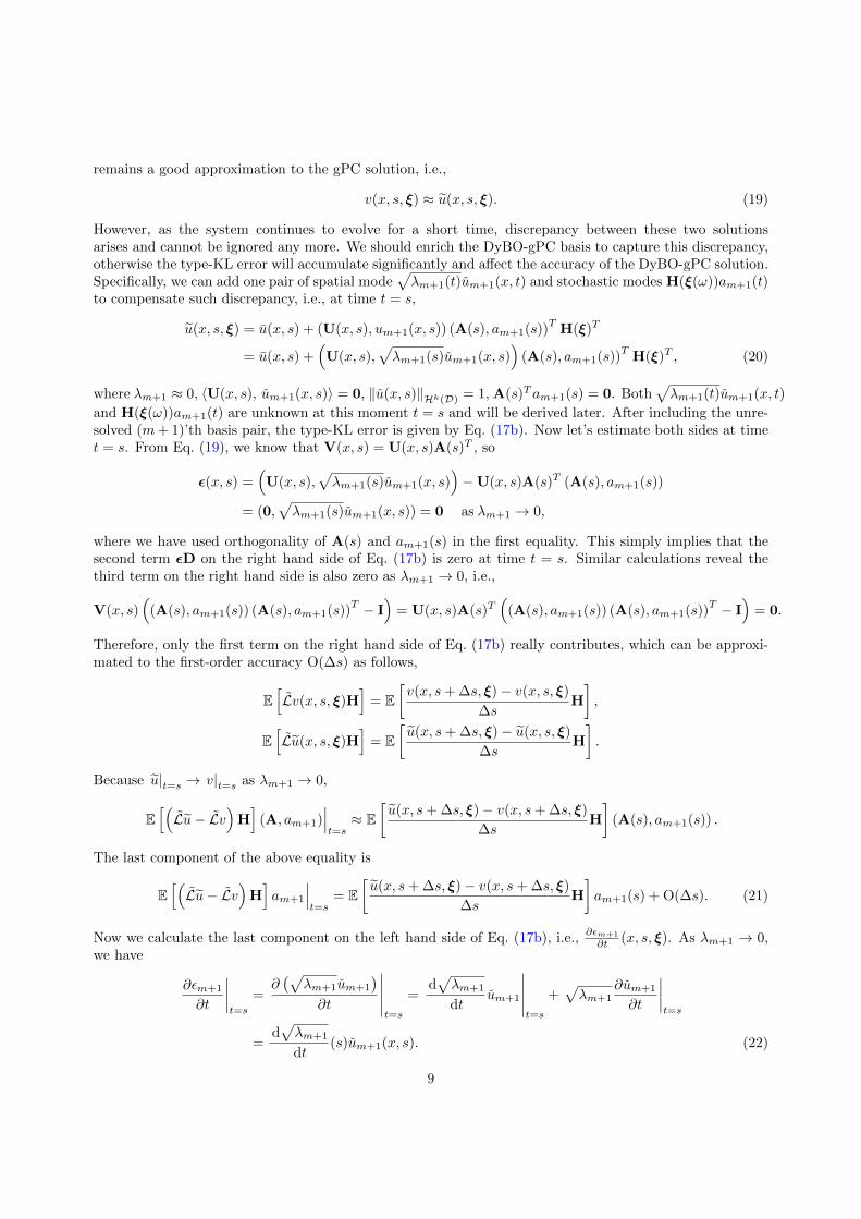
However, as the system continues to evolve for a short time, discrepancy between these two solutionsarises and cannot be ignored any more. We should enrich the DyBO-gPC basis to capture this discrepancy,otherwise the type-KL error will accumulate significantly and affect the accuracy of the DyBO-gPC solution.Specifically, we can add one pair of spatial mode
√λm+1(t)um+1(x, t) and stochastic modes H(ξ(ω))am+1(t)
to compensate such discrepancy, i.e., at time t = s,
u(x, s, ξ) = u(x, s) + (U(x, s), um+1(x, s)) (A(s), am+1(s))T
H(ξ)T
= u(x, s) +(U(x, s),
√λm+1(s)um+1(x, s)
)(A(s), am+1(s))
TH(ξ)T , (20)
where λm+1 ≈ 0, 〈U(x, s), um+1(x, s)〉 = 0, ‖u(x, s)‖Hk(D) = 1, A(s)Tam+1(s) = 0. Both√λm+1(t)um+1(x, t)
and H(ξ(ω))am+1(t) are unknown at this moment t = s and will be derived later. After including the unre-solved (m+ 1)’th basis pair, the type-KL error is given by Eq. (17b). Now let’s estimate both sides at timet = s. From Eq. (19), we know that V(x, s) = U(x, s)A(s)T , so
ε(x, s) =(U(x, s),
√λm+1(s)um+1(x, s)
)−U(x, s)A(s)T (A(s), am+1(s))
= (0,√λm+1(s)um+1(x, s)) = 0 as λm+1 → 0,
where we have used orthogonality of A(s) and am+1(s) in the first equality. This simply implies that thesecond term εD on the right hand side of Eq. (17b) is zero at time t = s. Similar calculations reveal thethird term on the right hand side is also zero as λm+1 → 0, i.e.,
V(x, s)(
(A(s), am+1(s)) (A(s), am+1(s))T − I
)= U(x, s)A(s)T
((A(s), am+1(s)) (A(s), am+1(s))
T − I)
= 0.
Therefore, only the first term on the right hand side of Eq. (17b) really contributes, which can be approxi-mated to the first-order accuracy O(∆s) as follows,
E[Lv(x, s, ξ)H
]= E
[v(x, s+ ∆s, ξ)− v(x, s, ξ)
∆sH
],
E[Lu(x, s, ξ)H
]= E
[u(x, s+ ∆s, ξ)− u(x, s, ξ)
∆sH
].
Because u|t=s → v|t=s as λm+1 → 0,
E[(Lu− Lv
)H]
(A, am+1)∣∣∣t=s≈ E
[u(x, s+ ∆s, ξ)− v(x, s+ ∆s, ξ)
∆sH
](A(s), am+1(s)) .
The last component of the above equality is
E[(Lu− Lv
)H]am+1
∣∣∣t=s
= E[u(x, s+ ∆s, ξ)− v(x, s+ ∆s, ξ)
∆sH
]am+1(s) + O(∆s). (21)
Now we calculate the last component on the left hand side of Eq. (17b), i.e., ∂εm+1
∂t (x, s, ξ). As λm+1 → 0,we have
∂εm+1
∂t
∣∣∣∣t=s
=∂(√
λm+1um+1
)∂t
∣∣∣∣∣t=s
=d√λm+1
dtum+1
∣∣∣∣∣t=s
+√λm+1
∂um+1
∂t
∣∣∣∣t=s
=d√λm+1
dt(s)um+1(x, s). (22)
9

t t+ ∆T t+ 2∆T t+ 3∆TTime
s = t+ ∆TRemoval of i’th pair
λiλmax
< ηuDyBO
uDyBO
uDyBO
ugPC
No Removal
∆u ≈√θ1w1(x)bT1H
uDyBO
Addition of new mode pairs
s+ ∆s
Figure 1: Illustration of strategies of adding and removing basis pairs.
Combining the above discussion, we have the following equality from Eq. (17),
d√λm+1
dt(s)um+1(x, s) ≈ E
[u(x, s+ ∆s, ξ)− v(x, s+ ∆s, ξ)
∆sH
]am+1(s). (23)
Now consider the KL expansion of the solution discrepancy at time t = s+ ∆s, i.e.,
∆u(x, s+ ∆s, ξ) = u(x, s+ ∆s, ξ)− v(x, s+ ∆s, ξ) =√θ1w1(x)bT1 HT + · · · , (24)
where θ1, w1(x) and Hb1 are the largest eigenvalue, normalized spatial and stochastic basis, respectively.The above equality implies that the growth rate of the largest unresolved eigenvalue λm+1 can be estimatedfrom the largest eigenvalue of ∆u. What’s more, a sensible choice of initial conditions for the newly addedbasis pair um+1(x, s) and am+1(s) would be the largest spatial and stochastic mode of ∆u(x, s+ ∆s, ξ), i.e.,√θ1w1(x) and Hb1. This strategy involves computation of gPC solutions for a short time ∆s, which can be
expensive. Instead of invoking such strategy every time step, we invoke such procedure every duration ∆T ,∆T ∆s. See Fig. 1 for illustrations.
We remark that a similar strategy of removing and adding spatial and stochastic basis pairs may bedeveloped for DyBO-gSC and DyBO-MC. The adaptive algorithm can be generalized to add more than onepair of spatial and stochastic basis at a time. The corresponding spatial and stochastic basis pairs can beobtained from the KL expansion of ∆u(x, t, ξ) in (24). Moreover, we note that the new spatial basis um+1
and new stochastic basis Ham+11(t) may not be perfectly orthogonal to other basis U(x, t) and HA at timet = s. Due to the bi-orthogonality-preserving property of the DyBO method (see Theorem 3.1 in [9]), suchdeviation from the bi-orthogonality will not be amplified.
5. Generalization of the DyBO method to a SPDE System
In addition to computational complexity analysis and adaptivity in changing basis number, the gener-alizations of the DyBO method will be another focus of this paper. In this section, we will discuss thegeneralization of the DyBO formulation for SPDE systems.
Many applications involve multiple physical fields, or physical components, for instance, the standardthree-dimensional incompressible Naiver-Stokes equations involve four physical components, three velocitycomponents along x-, y-, z-axis and pressure. When compressibility cannot be ignored, e.g., in aerodynamic[1], two additional components, typically density and temperature fields, get involved. Therefore, generaliz-ing the DyBO method for a system of time-dependent SPDEs is important and necessary. More precisely,
10

we consider a system of time-dependent SPDEs as follows:
∂ul∂t
(x, t, ω) = Ll u1, u2, · · · , uN , l = 1, 2, · · · , N, x ∈ D ⊂ Rd, t ∈ [0, T ], (25)
where each Ll is a stochastic differential operator acting on the physical components u1, u2, · · · , uN and Nis the total number of physical components. To simplify the notation, we omit the boundary condition andinitial condition for each component. When no ambiguity arises, we simply use shorthand notation
u = u1, u2, · · · , uN and Llu = Ll u1, u2, · · · , uN .
Unlike a single SPDE, randomness in (25) introduced through initial conditions, boundary conditions,stochastic forcing terms propagates not only in space and time, but also among different physical com-ponents. Randomness introduced by one physical component may affect other components. In general,different physical components may have different stochastic properties. Thus, using a common basis, suchas the orthonormal polynomial basis, may not be the most efficient way to represent the solution of astochastic system. The most compact representations in L2 sense are the KL expansions of each physicalcomponent, which is our starting point to derive the DyBO formulation for the SPDE system (25).
Consider the ml-term truncated KL expansion of the l’th physical component ul (x, t, ω),
ul = ul +
ml∑i=1
uliYli = ul + UlYTl ≈ ul, (26)
where Ul is a row vector of functions of spatial coordinate x and temporal coordinate t,
Ul(x, t) = (ul1(x, t), ul2(x, t), · · · , ulml(x, t)) ∈ R1×ml ,
and Yl is a row vector of random variables,
Yl(ω, t) = (Yl1(ω, t), Yl2(ω, t), · · · , Ylml(ω, t)) ∈ R1×ml .
With these preparations, we are now ready to derive our DyBO method for a system of SPDEs. Wefollow the steps in the derivation of DyBO method for a single SPDE (see Section 2 of [9]) by substitutingthe expansion (26) into the system (25) and using anti-symmetrization operators Q and Q to enforce thebi-orthogonality of the spatial and stochastic modes Ul and Yl of each physical component ul. Afterprojecting the growth rate of the spatial and stochastic modes ∂Ul
∂t and dYl
dt onto themselves, we arrive atthe generalized DyBO formulation for SPDE system (25) (see Cheng’s thesis [8] for details).
∂ul∂t
= E [Llu] , (27a)
∂Ul
∂t= −UlD
Tl + E
[LluYl
], (27b)
dYl
dt= −YlC
Tl +
⟨Llu, Ul
⟩Λ−1
Ul, (27c)
where l = 1, 2, · · · , N and u = u1, ..., uN. The matrices Cl’s and Dl’s can be solved from linear systems
Cl −Λ−1UlQ (ΛUl
Cl) = 0, (28a)
Dl −Q (Dl) = 0, (28b)
DTl + Cl = G∗l(ul,Ul,Yl), (28c)
with G∗l(ul,Ul,Yl) = Λ−1Ul
⟨UTl , E
[LluYl
]⟩∈ Rml×ml . The boundary conditions and initial conditions
for each physical components can be obtained correspondingly. We assume the randomnesses of the SPDEsystem follows the same distribution, then we can derive the DyBO-gPC formulation for the SPDE system.
11

For DyBO-gPC, the stochastic modes Yl are presented in the form of gPC expansions, i.e., Yl(ω, t) =H (ξ(ω)) Al, where Al ∈ RNp×ml . The DyBO-gPC formulation for each component is given by
∂ul∂t
= E [Llu] , (29a)
∂Ul
∂t= −UlD
Tl + E
[LluH
]Al, (29b)
dAl
dt= −AlC
Tl +
⟨E[HT Llu
], Ul
⟩Λ−1
Ul, (29c)
where Cl(t) and Dl(t) can be solved from
G∗l(ul,Ul,Yl) = Λ−1Ul
⟨UTl , E
[LluYl
]⟩= Λ−1
Ul
⟨UTl , E
[LluH
]⟩Al. (30)
Various theoretical results of the DyBO formulation for single SPDE, such as the preservation of bi-orthogonality and error analysis can be generalized to the DyBO formulation for a SPDE system. Thestrategies proposed for a single SPDE such as eigenvalues crossings and adding or removing basis pairs canalso be generalized to a system of SPDE. Similar results can be obtained for the DyBO-gSC version andDyBO-MC version. More details about the numerical implementation will be given in the next section.
6. Numerical Examples
Previous sections highlight the analytical aspects of the DyBO formulation and algorithm, this sectiondemonstrates its success by several numerical examples, each of which emphasizes and verifies some ofanalytical results in the previous sections. In the first example, a SPDE driven purely by stochastic forcesis considered, which shows the necessity of adaptivity in the DyBO method. More involved numericalexamples, such as spatially two-dimensional SPDE and/or a system of SPDEs, which require adaptivity,parallelization strategy and other numerical techniques, will also be reported in this section.
6.1. SPDE Purely Driven by Stochastic Forces
In the first numerical example, we consider the SPDE driven purely by a stochastic force f , i.e.,
∂u
∂t= Lu = f(x, t, ξ(ω)), x ∈ D = [0, 1], t ∈ [0, T ], (31)
where ξ = (ξ1, ξ2, · · · , ξr) are independent standard Gaussian random variables, i.e., ξi ∼ N (0, 1). A similarexample has been used in the first part of the paper [9] for eigenvalue crossing. Here we consider a differentstochastic force f to test the adaptive strategy proposed in Section 4. To construct such force, we consideran exact solution given in the following form,
u(x, t, ξ) = v(x, t) + V(x, t)ZT (ξ, t), (32)
where V(x, t) = V(x)WV(t)Λ12
V(t), Z(ξ, t) = Z(ξ)WZ(t), V(x) = (v1(x), · · · , vm(x)) with 〈vi(x), vj(x)〉 =
δij and Z(ξ) =(Z1(ξ), · · · , Zm(ξ)
)with E
[ZiZj
]= δij for i, j = 1, 2, · · · ,m. WV(t) and WZ(t) are m-by-
m orthonormal matrices, and Λ12
V(t) is a diagonal matrix. By differentiation, we can get the correspondingstochastic force
f =∂v
∂t+∂V
∂tZT + V
dZT
dt. (33)
12

By substituting the above equalities into DyBO-gPC system (7), we arrive at the DyBO-gPC formulationfor SPDE (31)
∂u
∂t=∂v
∂t, (34a)
∂U
∂t= −UDT +
(∂V
∂tWT
Z + VdWT
Z
dt
)E[ZTH
]A, (34b)
dA
dt= −ACT + E
[HT Z
]⟨WZ
∂VT
∂t+
dWZ
dtVT , U
⟩Λ−1
U , (34c)
and
G∗ (u,U,A) = Λ−1U
⟨U, ∂V
∂tWT
Z + VdWT
Z
dt
⟩E[ZTH
]A.
We consider a small system m = 3 and use the following settings,
V(x) =(√
2 sin(πx),√
2 sin(5πx),√
2 sin(9πx)), Z(x) = (H1(ξ1),H2(ξ1),H3(ξ1)) ,
WV(t) = PV
cos bVt − sin bVt 0sin bVt cos bVt 0
0 0 1
PTV, WZ(t) = PZ
cos bZt − sin bZt 0sin bZt cos bZt 0
0 0 1
PTZ,
where bV = 2.0, bZ = 2.0, PV and PZ are two orthonormal matrices generated randomly at the beginning,and H (ξ) = (H1(ξ1),H2(ξ1), · · · ,H5(ξ1)). To simulate the scenario where adding and removing mode pairsare necessary, we consider the following eigenvalues
Λ12
V = diag (3.0001 + sin(2πt), 2.0001 + sin(2πt), 1.0001 + sin(2πt)) ,
where λ3 becomes very small ∼ 10−8 near t = 0.25. See Fig. 2. We use this example to test the effectivenessof our first adaptive method based on the type-KL error analysis. When the adaptive strategy for addingmode pairs is invoked, it is crucial to know the growth rate of the largest unresolved eigenvalue and avoidadding such mode pair if it continues to be small in the near future ∆T . This is accomplished by computing
solutions by DyBO and gPC for a short time ∆s and estimating the growth rated√λm+1
dt from the differenceof the two solutions.
In Fig. 3, we verify the accuracy of such estimates, where the third mode pair is intentionally droppedat t = 0.2 when it becomes small (∼ 10−3) and never put back in the remaining computation. The solid
line is the exact growth rate of the largest unresolved eigenvalue, i.e., d√λ3
dt , while the dotted line is theestimate. In computations, we actually use different short time duration ∆s = 8δt, 4δt, 2δt, δt to verify theconvergence of such estimate. However, all of theses estimates cluster together and cannot be distinguishedfrom the figure. As we can see from Fig. 3, such estimates are very accurate when the largest unresolvedeigenvalue is indeed small and become less accurate when the largest unresolved eigenvalue is not so smallcompared to the resolved ones.
In Fig. 4, we consider the effect of the invoking frequency for adding mode pairs, i.e., 1∆T . If no mode pair
is added, the relative error of STD at t = 1.0 is about 26%. When the adaptive algorithm is incorporated,the error can be brought down to ≤ 1.5% depending on the invoking frequency. The threshold η in theadaptive algorithm is taken to be 10−4 and
√η = 10−2, so we see such difference is relatively marginal. We
will continue to demonstrate the effectiveness of the adaptive algorithm in more involved numerical examplesin the following subsections.
6.2. 2D Stochastic Flow
As a model to test numerically the proposed DyBO formulation for a spatially two-dimensional nonlinearSPDE, we consider the incompressible Navier-Stokes equations driven by stochastic forces. Specifically, we
13

0 0.1 0.2 0.3 0.4 0.5 0.6 0.7 0.8 0.9 110
−8
10−6
10−4
10−2
100
102
λ1
λ2
λ3
λ3 ≈ 10−8
Figure 2: Eigenvalues are plotted as function of time. λ3 becomes small near t = 0.25.
0 0.1 0.2 0.3 0.4 0.5 0.6 0.7 0.8 0.9 10
2
4
6
8
Smallest mode removed here
Figure 3: Change rate of the largest unresolved eigenvalue d√λ3
dt . Solid line is the exact solution, while thedotted line are computed the adaptive algorithm based on type-KL error analysis.
0.2 0.3 0.4 0.5 0.6 0.7 0.8 0.9 1
10−12
10−10
10−8
10−6
10−4
10−2
100
No Mode Added
20 Iterations
40 Iterations
60 Iterations
80 IterationsSmall modes removed
New modes added
26%
1.1%0.2%
Figure 4: L2 relative errors of STD given by DyBO with adding or removing basis pairs.
14

10
1
x
hy
hx
y
f(x,y, t) = (σ1(x,y)B1(t), σ2(x,y)B2(t))
Stochastic force
(a) Diagram of flow domain
0 0.2 0.4 0.6 0.80
0.1
0.2
0.3
0.4
0.5
0.6
0.7
0.8
0.9
−18
−16
−14
−12
−10
−8
−6
−4
−2
0
(b) Initial vorticity field
Figure 5: Stochastic flows driven by stochastic force f in 2D unit square.
consider the stochastic flow in an unit square, i.e., D = [0, 1]× [0, 1], with periodic boundary conditions onboth spatial directions x and y (see Fig. 5a). The governing equation of this stochastic flow is the StochasticNavier-Stokes equations (SNSEs). For spatially two-dimensional incompressible flow problems, it is moreconvenient to use the vorticity-stream function formulation. The vorticity-stream function formulation givesw = ∂v
∂x −∂u∂y and ψ, with velocity u = ∂ψ
∂y and v = −∂ψ∂x . The vorticity-stream formulation is given by
∂w
∂t= Lw = −
(u∂
∂x+ v
∂
∂y
)w + ν∆w +
(∂f2
∂x− ∂f1
∂y
), (35)
−∆ψ = w, (36)
u =∂ψ
∂y, v = −∂ψ
∂x. (37)
We assume the randomness is given in terms of r independent standard Gaussian random variables, ξ =(ξ1, ξ2, · · · , ξr), and the initial vorticity is deterministic, i.e., w(x, y, 0, ξ) = w(x, y). That is to say, therandomness is injected into the system only through the stochastic force f = (f1, f2). In the followingnumerical example, we choose ν = 2.0× 10⁻⁴ and adopt the initial vorticity field used in [14, 22],
w(x, y) = const− 1
2δ1exp
(−I(x)(y − 0.5)2
2δ21
),
where I(x) = 1 + δ2 (cos(4πx)− 1) and the constant is taken such that∫D w dx dy = 0. δ1 = 0.025 and
δ2 = 0.3, so the initial vorticity concentrates in a narrow band along y = 0.5 as shown in Fig. 5b, whichmodels a perturbed flat vortex sheet in the limit that δ1 → 0. For the driving stochastic force f , we consideran approximated version of Brownian force f = (σ1(x, y)B1(t), σ2(x, y)B2(t)) (see [8, 9, 22, 14] for the detailsof the construction)(
∂f2
∂x− ∂f1
∂y
)= −∂σ1
∂y
4∑i=1
1√TMi
(t
T
)ξi +
∂σ2
∂x
8∑i=5
1√TMi−4
(t
T
)ξi = FHT . (38)
The functions σ1 and σ2 are chosen such that
∂σ1
∂y= 0.3π cos (2πx) cos (2πy) ,
∂σ2
∂x= 0.3π sin (2πx) sin (2πy) .
15

The derivations of gPC or DyBO-gPC formulations of SNSE is standard. By considering the gPCexpansion w = w + WHT , we can derive the gPC formulation of SNSE (35),
∂w
∂t= ν∆w −D(u,v)w −D(U,V)W, (39a)
∂W
∂t= ν∆W −D(u,v)W
T −D(U,V)w −(D(uα,vα)wβT
(H)αβγ
)1×γ
+ F, (39b)
where D(·,·) (·) is a generalized material derivative defined as follows. For a scalar or row-vector field θ underscalar or row-vector velocity field u and v,
D(u,v)θ =
u∂θ
∂x+ v
∂θ
∂y, u, v, θ are scalars,
u∂θ
∂x+ v
∂θ
∂y, u, v are scalars and θ is a row vector,
∂θ
∂xu+
∂θ
∂yv, u, v are row vectors and θ is a scalar,
u∂θT
∂x+ v
∂θT
∂y, u, v, θ are row vectors,
(40)
where u and v can be row vectors of the same length and the right hand side is understood in the usualsense of vector-vector multiplications or scalar-vector multiplications.
The DyBO-gPC formulation of SNSE (35) can be obtained by considering the m-term truncated KLexpansion w = w + WATHT , see Appendix A for more details about its derivation.
∂w
∂t= ν∆w −D(u,v)w −D(U,V)W, (41a)
∂W
∂t= −WDT
w +[ν∆W −D(u,v)W −D(U,V)w
]−[D(ui,vi)wjAαiAβjAγkT
(H)αβγ
]1×k
+ FA, (41b)
dA
dt= A
(−CT
w +⟨ν∆WT −
(D(u,v)W
)T − (D(U,V)w)T, W
⟩Λ−1W
)−[T
(W)ijk AαiAβjT
(H)αβγ
]γ×k
Λ−1W +
⟨FT , W
⟩Λ−1W , (41c)
where matrices Cw and Dw can be solved from the linear system (4) from G∗w,
ΛWG∗w =⟨WT , ν∆W −D(u,v)W −D(U,V)w
⟩−[T
(W)ijk AαiAβjAγlT
(H)αβγ
]k×l
+⟨WT , F
⟩A.
For notation compactness, the spatial basis W in DyBO-gPC formulation should not be confused with thenotation in gPC formulation (39).
Both the gPC system and DyBO-gPC systems are numerically solved by the fourth-order RK methodwith time step ∆t = 10−3 on a 128× 128 spatial grid. The pseudo-spectral method with the 36-dealiasingrule [15, 16] is used to compute spatial derivatives. Various numerical results are presented in the following.
Verification of Complexity Analysis. Clearly, SNSE (35) is a quadratic nonlinear PDE driven bystochastic forces, so the computational complexity analysis in Section 3 is applicable. Before presentingcomputational results, we first verify the complexity analysis, i.e., Eq. (15). To this end, we record the walltime of a single time step when the gPC system (39) or the DyBO-gPC system (41) is numerically integratedby the fourth-order Runge-Kutta method. For Np = 80, 100, 120 and m = 4, 8, 12, 16, the computationaltimes are summarized in Table 4. To improve the accuracy of recorded wall times, we actually compute theaverage wall time of 10 time iterations.
In Table 4, the exponents α and β in Eq. (15) are estimated by linear regression. The last column useswall times corresponding to m = 8, 12, 16 , while the second to last column uses all four values of m. As we
16

101
10−2
10−1
100
NP=80
NP=100
NP=120
Figure 6: Wall times of a single RK step of the DyBO-gPC system. The horizontal axis is the number ofmode pairs, m.
can see from the fourth column of the table, the computational time is relatively small when m = 4. In thiscase, the dominant terms in our previous analysis may not truly dominate other terms and some inevitableprogramming overheads, such as memory allocations and function calling overheads, may kick in. In Fig. 6accompanying Table 4, the computational times corresponding to m = 8, 12, 16 align nicely into a straightline for each Np = 80, 100, 120, respectively, but the computational times corresponding to m = 4 drift up.If we remove these points from our fitting, the linear regression estimate of the exponent α in Eq. (15) wouldbe approximately equal to 2.73, close to the theoretically predicated value 3.
As we mentioned in Remark 3.1, T(H) is very sparse when Hermite polynomials are used for Gaussianrandom variables. In Table 4, we also report the wall times of gPC in the second and third columns,respectively, depending on whether such sparsity is explored or not in the numerical implementation of gPCmethods. Clearly, the computational cost is significantly smaller if such sparsity is considered. However,we may not have such luxury for arbitrary non-Gaussian random variables, i.e., general distributions. Inthe last two rows of Table 4, the exponent β is estimated by linear regression, respectively, when sparsity isexplored or not. The last row gives ∼ 2.9 for the exponent β confirming our analysis in Eq. (15).
gPC (sec) DyBO-gPC (sec) αNp Sparse Non-Sparse m = 4 m = 8 m = 12 m = 16 α1 α2
80 17.242 772.10 0.3946 1.6238 4.8850 10.5483 2.3670 2.7006100 26.302 1482.7 0.4221 1.5666 4.9577 10.7119 2.3334 2.7779120 36.440 2558.3 0.4246 1.6567 5.0451 10.8200 2.3342 2.7099
β - Sparse 1.6621 1.8056 1.7683 1.7844ββ - Non-Sparse 2.7683 2.9117 2.8744 2.8905
Table 4: Comparison of wall times of a single RK step of gPC and DyBO-gPC systems.
Numerical Errors of DyBO-gPC. The number of polynomial basis functions Hα grows exponentiallyfast as the number of random variables r and the total order p increase. The scheme of sparse truncationproposed in Luo’s thesis [22] (see also [14]) proves to be a relatively effective method to alleviate the situation.In the following computation, we follow this scheme and choose a multi-index set J obtained from a sparsetruncation of the multi-index set J3
8,
J =α ∈ J3
8 and if |α| = 3, then α2 ≤ 2, α3 ≤ 1, α4 ≤ 1, α6 ≤ 2, α7 ≤ 1, α8 ≤ 1\ 0 ,
which still results in total 130 multi-indices!The mean and the STD of the vorticity field and the first four spatial modes in the KL expansion of the
vorticity field at time t = 1.0 are given in Fig. 7 and Fig. 8, respectively. In both figures, the results by
17

0 0.2 0.4 0.6 0.80
0.1
0.2
0.3
0.4
0.5
0.6
0.7
0.8
0.9
0 0.2 0.4 0.6 0.80
0.1
0.2
0.3
0.4
0.5
0.6
0.7
0.8
0.9
0 0.2 0.4 0.6 0.80
0.1
0.2
0.3
0.4
0.5
0.6
0.7
0.8
0.9
0 0.2 0.4 0.6 0.80
0.1
0.2
0.3
0.4
0.5
0.6
0.7
0.8
0.9
−15
−10
−5
0
0.5
1
1.5
2
2.5
3
3.5
4
4.5
5
5.5
−15
−10
−5
0
0.5
1
1.5
2
2.5
3
3.5
4
4.5
5
5.5
(a) Mean
0 0.2 0.4 0.6 0.80
0.1
0.2
0.3
0.4
0.5
0.6
0.7
0.8
0.9
0 0.2 0.4 0.6 0.80
0.1
0.2
0.3
0.4
0.5
0.6
0.7
0.8
0.9
0 0.2 0.4 0.6 0.80
0.1
0.2
0.3
0.4
0.5
0.6
0.7
0.8
0.9
0 0.2 0.4 0.6 0.80
0.1
0.2
0.3
0.4
0.5
0.6
0.7
0.8
0.9
−15
−10
−5
0
0.5
1
1.5
2
2.5
3
3.5
4
4.5
5
5.5
−15
−10
−5
0
0.5
1
1.5
2
2.5
3
3.5
4
4.5
5
5.5
(b) Mean
0 0.2 0.4 0.6 0.80
0.1
0.2
0.3
0.4
0.5
0.6
0.7
0.8
0.9
0 0.2 0.4 0.6 0.80
0.1
0.2
0.3
0.4
0.5
0.6
0.7
0.8
0.9
0 0.2 0.4 0.6 0.80
0.1
0.2
0.3
0.4
0.5
0.6
0.7
0.8
0.9
0 0.2 0.4 0.6 0.80
0.1
0.2
0.3
0.4
0.5
0.6
0.7
0.8
0.9
−15
−10
−5
0
0.5
1
1.5
2
2.5
3
3.5
4
4.5
5
5.5
−15
−10
−5
0
0.5
1
1.5
2
2.5
3
3.5
4
4.5
5
5.5
(c) STD
0 0.2 0.4 0.6 0.80
0.1
0.2
0.3
0.4
0.5
0.6
0.7
0.8
0.9
0 0.2 0.4 0.6 0.80
0.1
0.2
0.3
0.4
0.5
0.6
0.7
0.8
0.9
0 0.2 0.4 0.6 0.80
0.1
0.2
0.3
0.4
0.5
0.6
0.7
0.8
0.9
0 0.2 0.4 0.6 0.80
0.1
0.2
0.3
0.4
0.5
0.6
0.7
0.8
0.9
−15
−10
−5
0
0.5
1
1.5
2
2.5
3
3.5
4
4.5
5
5.5
−15
−10
−5
0
0.5
1
1.5
2
2.5
3
3.5
4
4.5
5
5.5
(d) STD
Figure 7: Mean and STD of the vorticity field at time t = 1.0. The left column is computed by DyBO-gPC,while the right column is computed by gPC.
our DyBO-gPC method with m = 8 are given in the left column and compared to the results by the gPCmethod in the right column. The results are almost indistinguishable. We further confirm the convergenceof DyBO-gPC to gPC by plotting the relative errors of both mean and STD of the vorticity field as functionsof time in the top two subplots of Fig. 9.
In the same figure, we also report the relative errors as functions of time when the adaptive strategy ofadding and/or removing basis pairs is enacted. Two numerical examples are provided: one starts with fourbasis pairs, i.e., m0 = 4 and the other starts with six basis pairs, i.e., m0 = 6. In Fig. 9c, the number ofbasis pairs in the DyBO-gPC method is plotted against time t. Because of the special form of the stochasticforce f considered in this numerical example, the randomness is only introduced through low-order gPCcoefficients and then spread to the mean and other high-order gPC coefficients. At the beginning of theevolution of the stochastic flow, the randomness is not strong and the adaptive algorithm finds no needto add new basis pairs before time t = 0.35. As the system evolves, the randomnesses get strong throughinteractions among different basis pairs and the adaptive algorithm automatically adds more basis pairswhen necessary.
Avoiding Selection of Multi-index Set J. The gPC method suffers greatly from the curse ofdimensionality. In the above numerical example, we use low-order (≤ 3) polynomials and also the sparsetruncation technique to further reduce the size of multi-index set J, which still results in a set of 130polynomials. It takes more than 8 hour of wall time to numerically integrate the gPC system from t = 0.0to t = 1.0. Adaptive gPC methods try to include only the most important gPC coefficients wα in thecomputation, i.e., a selection of multi-index set J.
In Fig. 10a, we plot the energy spectrum of the gPC solution at t = 1.0, i.e., the L2 norm of the gPCcoefficient wα, which does not decay monotonically. Index J is a multi-index set, so we do not have sufficientinformation and a good strategy, prior to the computation, to sort J and select the most important ones.
On the other hand, our DyBO method tracks the KL expansion of the true solution and automatically
18

0 0.2 0.4 0.6 0.80
0.2
0.4
0.6
0.8
0 0.2 0.4 0.6 0.80
0.2
0.4
0.6
0.8
0 0.2 0.4 0.6 0.80
0.2
0.4
0.6
0.8
0 0.2 0.4 0.6 0.80
0.2
0.4
0.6
0.8
0 0.2 0.4 0.6 0.80
0.2
0.4
0.6
0.8
0 0.2 0.4 0.6 0.80
0.2
0.4
0.6
0.8
0 0.2 0.4 0.6 0.80
0.2
0.4
0.6
0.8
0 0.2 0.4 0.6 0.80
0.2
0.4
0.6
0.8
−5
0
5
−5
0
5
−1
0
1
2
−1
0
1
2
−2
−1
0
1
2
−2
−1
0
1
2
−1
0
1
−1
0
1
(a) 1st spatial basis
0 0.2 0.4 0.6 0.80
0.2
0.4
0.6
0.8
0 0.2 0.4 0.6 0.80
0.2
0.4
0.6
0.8
0 0.2 0.4 0.6 0.80
0.2
0.4
0.6
0.8
0 0.2 0.4 0.6 0.80
0.2
0.4
0.6
0.8
0 0.2 0.4 0.6 0.80
0.2
0.4
0.6
0.8
0 0.2 0.4 0.6 0.80
0.2
0.4
0.6
0.8
0 0.2 0.4 0.6 0.80
0.2
0.4
0.6
0.8
0 0.2 0.4 0.6 0.80
0.2
0.4
0.6
0.8
−5
0
5
−5
0
5
−1
0
1
2
−1
0
1
2
−2
−1
0
1
2
−2
−1
0
1
2
−1
0
1
−1
0
1
(b) 2nd spatial basis
0 0.2 0.4 0.6 0.80
0.2
0.4
0.6
0.8
0 0.2 0.4 0.6 0.80
0.2
0.4
0.6
0.8
0 0.2 0.4 0.6 0.80
0.2
0.4
0.6
0.8
0 0.2 0.4 0.6 0.80
0.2
0.4
0.6
0.8
0 0.2 0.4 0.6 0.80
0.2
0.4
0.6
0.8
0 0.2 0.4 0.6 0.80
0.2
0.4
0.6
0.8
0 0.2 0.4 0.6 0.80
0.2
0.4
0.6
0.8
0 0.2 0.4 0.6 0.80
0.2
0.4
0.6
0.8
−5
0
5
−5
0
5
−1
0
1
2
−1
0
1
2
−2
−1
0
1
2
−2
−1
0
1
2
−1
0
1
−1
0
1
(c) 3rd spatial basis
0 0.2 0.4 0.6 0.80
0.2
0.4
0.6
0.8
0 0.2 0.4 0.6 0.80
0.2
0.4
0.6
0.8
0 0.2 0.4 0.6 0.80
0.2
0.4
0.6
0.8
0 0.2 0.4 0.6 0.80
0.2
0.4
0.6
0.8
0 0.2 0.4 0.6 0.80
0.2
0.4
0.6
0.8
0 0.2 0.4 0.6 0.80
0.2
0.4
0.6
0.8
0 0.2 0.4 0.6 0.80
0.2
0.4
0.6
0.8
0 0.2 0.4 0.6 0.80
0.2
0.4
0.6
0.8
−5
0
5
−5
0
5
−1
0
1
2
−1
0
1
2
−2
−1
0
1
2
−2
−1
0
1
2
−1
0
1
−1
0
1
(d) 4th spatial basis
0 0.2 0.4 0.6 0.80
0.2
0.4
0.6
0.8
0 0.2 0.4 0.6 0.80
0.2
0.4
0.6
0.8
0 0.2 0.4 0.6 0.80
0.2
0.4
0.6
0.8
0 0.2 0.4 0.6 0.80
0.2
0.4
0.6
0.8
0 0.2 0.4 0.6 0.80
0.2
0.4
0.6
0.8
0 0.2 0.4 0.6 0.80
0.2
0.4
0.6
0.8
0 0.2 0.4 0.6 0.80
0.2
0.4
0.6
0.8
0 0.2 0.4 0.6 0.80
0.2
0.4
0.6
0.8
−5
0
5
−5
0
5
−1
0
1
2
−1
0
1
2
−2
−1
0
1
2
−2
−1
0
1
2
−1
0
1
−1
0
1
(e) 1st spatial basis
0 0.2 0.4 0.6 0.80
0.2
0.4
0.6
0.8
0 0.2 0.4 0.6 0.80
0.2
0.4
0.6
0.8
0 0.2 0.4 0.6 0.80
0.2
0.4
0.6
0.8
0 0.2 0.4 0.6 0.80
0.2
0.4
0.6
0.8
0 0.2 0.4 0.6 0.80
0.2
0.4
0.6
0.8
0 0.2 0.4 0.6 0.80
0.2
0.4
0.6
0.8
0 0.2 0.4 0.6 0.80
0.2
0.4
0.6
0.8
0 0.2 0.4 0.6 0.80
0.2
0.4
0.6
0.8
−5
0
5
−5
0
5
−1
0
1
2
−1
0
1
2
−2
−1
0
1
2
−2
−1
0
1
2
−1
0
1
−1
0
1
(f) 2nd spatial basis
0 0.2 0.4 0.6 0.80
0.2
0.4
0.6
0.8
0 0.2 0.4 0.6 0.80
0.2
0.4
0.6
0.8
0 0.2 0.4 0.6 0.80
0.2
0.4
0.6
0.8
0 0.2 0.4 0.6 0.80
0.2
0.4
0.6
0.8
0 0.2 0.4 0.6 0.80
0.2
0.4
0.6
0.8
0 0.2 0.4 0.6 0.80
0.2
0.4
0.6
0.8
0 0.2 0.4 0.6 0.80
0.2
0.4
0.6
0.8
0 0.2 0.4 0.6 0.80
0.2
0.4
0.6
0.8
−5
0
5
−5
0
5
−1
0
1
2
−1
0
1
2
−2
−1
0
1
2
−2
−1
0
1
2
−1
0
1
−1
0
1
(g) 3rd spatial basis
0 0.2 0.4 0.6 0.80
0.2
0.4
0.6
0.8
0 0.2 0.4 0.6 0.80
0.2
0.4
0.6
0.8
0 0.2 0.4 0.6 0.80
0.2
0.4
0.6
0.8
0 0.2 0.4 0.6 0.80
0.2
0.4
0.6
0.8
0 0.2 0.4 0.6 0.80
0.2
0.4
0.6
0.8
0 0.2 0.4 0.6 0.80
0.2
0.4
0.6
0.8
0 0.2 0.4 0.6 0.80
0.2
0.4
0.6
0.8
0 0.2 0.4 0.6 0.80
0.2
0.4
0.6
0.8
−5
0
5
−5
0
5
−1
0
1
2
−1
0
1
2
−2
−1
0
1
2
−2
−1
0
1
2
−1
0
1
−1
0
1
(h) 4th spatial basis
Figure 8: The first four spatial basis at time t = 1.0. Top are computed by DyBO-gPC, while the bottomare computed by gPC.
0.2 0.3 0.4 0.5 0.6 0.7 0.8 0.9 10
0.01
0.02
0.03
0.04
0.05
0.2 0.3 0.4 0.5 0.6 0.7 0.8 0.9 10
0.05
0.1
0.15
0.2
0.2 0.3 0.4 0.5 0.6 0.7 0.8 0.9 14
6
8
10
12
14
m= 4
m= 8
m=12
m=16Adaptive m
0=4
Adaptive m0=6
m= 4
m= 8
m=12
m=16Adaptive m
0=4
Adaptive m0=6
Adaptive m0=4
Adaptive m0=6
(a) Mean0.2 0.3 0.4 0.5 0.6 0.7 0.8 0.9 10
0.01
0.02
0.03
0.04
0.05
0.2 0.3 0.4 0.5 0.6 0.7 0.8 0.9 10
0.05
0.1
0.15
0.2
0.2 0.3 0.4 0.5 0.6 0.7 0.8 0.9 14
6
8
10
12
14
m= 4
m= 8
m=12
m=16Adaptive m
0=4
Adaptive m0=6
m= 4
m= 8
m=12
m=16Adaptive m
0=4
Adaptive m0=6
Adaptive m0=4
Adaptive m0=6
(b) STD
0.2 0.3 0.4 0.5 0.6 0.7 0.8 0.9 10
0.01
0.02
0.03
0.04
0.05
0.2 0.3 0.4 0.5 0.6 0.7 0.8 0.9 10
0.05
0.1
0.15
0.2
0.2 0.3 0.4 0.5 0.6 0.7 0.8 0.9 14
6
8
10
12
14
m= 4
m= 8
m=12
m=16Adaptive m
0=4
Adaptive m0=6
m= 4
m= 8
m=12
m=16Adaptive m
0=4
Adaptive m0=6
Adaptive m0=4
Adaptive m0=6
(c) m
Figure 9: The L2 relative errors of mean and STD of vorticity field computed by DyBO. The errors areplotted as functions of time in the top two figures, while the numbers of basis pairs used in the adaptivestrategy are given in the last figure.
19

0 20 40 60 80 100 120 14010
−4
10−3
10−2
10−1
100
101
gPC ‖wα‖L2
(a) Unsorted energy spectrum of the gPC solution
0 10 20 30 40 50 6010
−2
10−1
100
101
gPC ‖wα‖L2
DyBO ‖wi‖L2
(b) Sorted energy spectrum.
Figure 10: Comparison of energy spectrum of gPC and DyBO solutions at time t = 1.0.
includes only the most important ones. Furthermore, the KL expansion is known to provide the mostcompact representation of a second-order stochastic process, so the energy spectrum of the DyBO solution,i.e., the L2 norm of the DyBO-gPC coefficient wi, i = 1, 2, ...,m, has a faster decay rate even compared tothe sorted energy spectrum of gPC solution (see Fig. 10b). This difference in the decay rate implies thatour method leads to a smaller system to solve, leading to less computational cost.
To further illustrate and understand the benefits of the DyBO method, we consider a little “stronger”stochastic force (
∂f2
∂x− ∂f1
∂y
)= −∂σ1
∂y
4∑i=1
it
Tξi +
∂σ2
∂x
8∑i=5
(i− 4)t
T
(t
T
)ξi. (42)
With this stochastic force, the sorted energy spectrum of both gPC and DyBO solutions along with thesquare roots of eigenvalues are plotted in Fig. 11a. Clearly, the energy spectrum of DyBO decays muchfaster than that of gPC.
Once the gPC coefficients wα’s are sorted in the descending order in L2 norm, we can use the firstseveral gPC coefficients, i.e., the most important ones, to compute a solution and compare with the exactone. The relative errors of STD computed by this procedure are plotted in Fig. 11b against the number ofgPC coefficients.
At the first glance, this procedure may seem effective. But we would like to point out that the multi-indices α’s corresponding to the most important gPC coefficients are in general not known prior to thebeginning of computations. What’s more, such set of multi-indices may change with respect to time t,making the selection of an effective multi-index set J even harder. Moreover, the less important gPCcoefficients excluded from the gPC system may induce additional errors when we solve the system whichonly includes the most important ones. In fact, we observe that the solution obtained by this procedure isless accurate than that by our DyBO method with the same number of basis pairs, as shown in Fig. 11b.With only 8 basis pairs, our DyBO method achieves the same accuracy (∼ 0.5%) as that by gPC methodwith 60 gPC coefficients. By using Table 4, we can estimate speedup in this case. When the sparsity oftensor TH is not exploited in the numerical implementation of gPC, the speedup is ∼ 200X (327.8sec v.s.1.6567sec per time iteration). When the sparsity is exploited (see Remark 3.1 in Section 3.2), the speedupis ∼ 6X (10.628sec v.s. 1.6567sec per time iteration). Fig. 11a also confirms numerically that our DyBOmethod can accurately recover the eigenvalues in the KL expansion.
Looking into the stochastic basis Y = HA reveals the origin of the fast error decay in our DyBO-gPC method. In Fig. 12, we plot the stochastic basis computed by DyBO in the second figure and onesrecovered from the gPC solution in the third figure, respectively. Clearly, each stochastic basis Yi is a linearcombination of several, possibly many, gPC basis. Therefore, unlike gPC methods, where the stochasticbasis H is fixed and does not change with time, the DyBO method aggregates the polynomial basis and
20

0 10 20 30 40 50 6010
−3
10−2
10−1
100
DyBO ‖wi‖L2
√λi
gPC ‖wα‖L2
(a) (Sorted) Energy spectrum of the gPC andDyBO solutions.
0 10 20 30 40 50 6010
−3
10−2
10−1
100
gPC
DyBO
∼ e−0.065NP
∼ e−0.62m
(b) Relative errors of STD computed by gPCand DyBO methods
Figure 11: Comparisons of gPC and DyBO methods.
2 4 6 8
20
40
60
80
100
120
2 4 6 8
20
40
60
80
100
120−0.6
−0.4
−0.2
0
0.2
0.4
−0.6
−0.4
−0.2
0
0.2
0.4
(a) DyBO
2 4 6 8
20
40
60
80
100
120
2 4 6 8
20
40
60
80
100
120−0.6
−0.4
−0.2
0
0.2
0.4
−0.6
−0.4
−0.2
0
0.2
0.4
(b) gPC
Figure 12: Stochastic basis computed by DyBO and gPC.
21

forms a more efficient stochastic basis Y. Moreover, this set of stochastic basis is automatically adapted intime.
6.3. 2D Stochastic Flow Driven by Buoyance Force
As a model to test numerically the generalized DyBO formulation for a system of time-dependent SPDEs,we consider the Navier-Stokes equations whose velocity components are driven by both stochastic forces andbuoyancy forces due to small density difference induced by temperature variations. Specifically, we considerthe stochastic flow in an unite square, i.e., D = [0, 1] × [0, 1], with periodic boundary conditions on bothspatial directions. See Fig. 13a.
10
1
Periodic boundary condition
g
y
x
Perio
dic
bou
nary
condition
(a)
0 0.2 0.4 0.6 0.80
0.1
0.2
0.3
0.4
0.5
0.6
0.7
0.8
0.9
0
0.1
0.2
0.3
0.4
0.5
0.6
0.7
0.8
0.9
(b)
Figure 13: Stochastic flow driven by stochastic force and buoyancy force due to Boussinesq approximation.On the left: Diagram of the stochastic flow in an unit square. The gravity is downward parallel to y-axis andperiodic boundary conditions are assumed on both x and y directions. On the right, the initial temperaturefield is plotted, while the initial vorticity is uniformly zero.
The temperature field is not spatially uniform and causes variations of the density field. Such variationsare small because we assume the thermal expansion coefficient is very small. The induced buoyancy force maydrive the flow motion in addition to external stochastic forces. Here, we adopt the Boussinesq approximationto model such buoyancy force. The governing SPDE of such stochastic flow in Fig. 13a is the StochasticNavier-Stokes equations (SNSE)
∂θ
∂t+ u
∂θ
∂x+ v
∂θ
∂y= κ∆θ, (43a)
ut + u · ∇u = ν4u−∇p+ f + F (43b)
∇ · u = 0, (43c)
where the viscosity ν = 2.0 × 10⁻⁴ and the thermal diffusivity κ = 2.0 × 10⁻⁴ . θ is temperature field,u = (u, v) is the velocity field, p is the pressure, f = (f1, f2) is the zero-mean stochastic force vector andF = (0, µgθ) is the buoyancy force, where µ is the thermal expansion coefficient, g is the gravity of Earthand scaled gravity µg = 11.31 (see [7] for more details).
At the first glance, this numerical example is similar to the one in Section 6.2 except introducing theadditional temperature field and gravity effect. However, the stochastic flow is very different from the oneconsidered previously for the following reason. We see that the buoyancy force depends on the gradient oftemperature field and is actually a stochastic force. In other words, the stochastic flow considered in thissection is driven by two kinds of stochastic forces: one “external” stochastic force injecting randomness fromthe ambient environment into the unit square and one “internal” stochastic force feeding randomness back
22

to the system, from temperature component to vertical velocity component. Such stochastic flow providesa severe test model for our generalized DyBO methods.
Like the previous numerical example, it is convenient to consider the vorticity-stream function formulationin the standard form defined in the system of SPDEs (25),
∂θ
∂t= Lθ θ, w = −
(u∂
∂x+ v
∂
∂y
)θ + κ∆θ, (44a)
∂w
∂t= Lw θ, w = −
(u∂
∂x+ v
∂
∂y
)w + ν∆w +
(∂f2
∂x− ∂f1
∂y
)+ µg
∂θ
∂x. (44b)
Consider the finite-term KL expansion of the solutions of SNSE (44),
θ = θ + θYT = θ + θATHT , (45a)
w = w + WZT = w + WBTHT , (45b)
where row vectors θ = (θ1, θ2, · · · , θmθ ) and W = (w1, w2, · · · , wmw), and matrices A ∈ RNp×mθ andB ∈ RNp×mw . We write basis number vector m = (mθ,mW). By substituting the above expansion intoEq. (29), we obtain the DyBO-gPC formulation for SNSE (44) (see Appendix A for details). The system ofequations for the temperature component are
∂θ
∂t= κ∆θ −D(u,v)θ −D(U,V)
(θATB
), (46a)
∂θ
∂t= −θDT
θ + κ∆θ −D(u,v)θ −D(U,V)θBTA
−[D(ui,vi)θjBαiAβjAγkT
(H)αβγ
]1×k
, (46b)
dA
dt= A
(−CT
θ + κ⟨
∆θT , θ⟩
Λ−1θ −
⟨(D(u,v)θ
)T, θ⟩
Λ−1θ
)−B
⟨(D(U,V)θ
)T, θ⟩
Λ−1θ −
[T
(θ)ijkBαiAβjT
(H)αβγ
]γ×k
Λ−1θ , (46c)
where matrices Cθ and Dθ can be solved from the linear system (4) from G∗θ,
ΛθG∗θ = κ⟨θT , ∆θ
⟩−⟨θT , D(u,v)θ
⟩−⟨θT , D(U,V)θ
⟩BTA
−[T
(θ)ijkBαiAβjAγlT
(H)αβγ
]k×l
. (47)
The system of equations for the vorticity component are
∂w
∂t=
(ν∆w −D(u,v)w + µg
∂θ
∂x
)−D(U,V)W, (48a)
∂W
∂t= −WDT
w +[ν∆W −D(u,v)W −D(U,V)w
]+ µg
∂θ
∂xATB
−[D(ui,vi)wjBαiBβjBγkT
(H)αβγ
]1×k
+ FB, (48b)
dB
dt= B
(−CT
w +⟨ν∆WT −
(D(u,v)W
)T − (D(U,V)w)T, W
⟩Λ−1
W
)+ µgA
⟨∂θT
∂x, W
⟩Λ−1
W −[T
(W)ijk BαiBβjT
(H)αβγ
]γ×k
Λ−1W +
⟨FT , W
⟩Λ−1
W , (48c)
where matrices Cw and Dw can be solved from the linear system (4) from G∗w,
ΛWG∗w =⟨WT , ν∆W −D(u,v)W −D(U,V)w
⟩+
⟨WT , µg
∂θ
∂x
⟩ATB−
[T
(W)ijk BαiBβjBγlT
(H)αβγ
]k×l
+⟨WT , F
⟩B. (49)
23

Both the gPC system and the DyBO-gPC system are numerically integrated by the fourth-order RK methodwith a time step ∆t = 10−3. Unlike the stochastic flow only driven by the stochastic force in the previousnumerical example, we found by numerical experiments a higher-resolution spatial grid is necessary to resolvesome fine structures. Thus, we use 256 × 256 spatial grid in the numerical simulations. Computations onhigher resolution grid, 512× 512, are also performed for the gPC method to make sure that the solution isindeed well-resolved. The pseudo-spectral method with the 36-dealiasing rule [15, 16] is used to computespatial derivatives. For the DyBO method, the gPC solution at ∆T0 = 0.2 are used as initial conditions.Different values of ∆T0, such as 0.1 and 0.15, have also been used and no significant differences have beenfound. Here, we use the sparse truncation technique and choose the multi-index set
J =α ∈ J3
8 and if |α| = 3, then α2 ≤ 2, α3 ≤ 1, α4 ≤ 1, α6 ≤ 2, α7 ≤ 1, α8 ≤ 1\ 0 .
Both initial vorticity and temperature field are assumed to be deterministic. In this example, we areprimarily interested in the combined effect of stochastic force f and the stochastic buoyancy force, so thevorticity is assumed to be zero initially. We adopt the initial temperature field from [7],
θ(x, y, 0, ξ) = θ(x, y) =1
2Hδ1 (ylb(x)− y) +
1
2Hδ1 (yub(x)− y) , (50)
where ylb(x) = 12 − δ2 − δ3y0(x), yub(x) = 1
2 + δ2 + δ3y0(x), y0(x) = 1 + sin(2π(x+ 3
4
)), and the modified
Heaviside step function Hε(z) = x+ε2ε + 1
2π sin(πxε
). In Fig. 13b, the initial temperature field θ is plotted.
In the first numerical example, we choose basis number vector m = (7, 8). In Fig. 14, STD fields ofvorticity and temperature are plotted at time t = 1.0 with the results by DyBO in the left column and onesby gPC in the right column. We also compare the spatial basis of vorticity and temperature, W and θ,given by DyBO and gPC at time t = 1.0, respectively (not shown here, see [8]). These results confirm thatthe solutions given by DyBO are not only a good approximation to the solution given by gPC, but alsotrack directly the KL expansion of the SPDE solution.
To further study the numerical convergence of our DyBO method, we choose another two basis numbervectors, m = (3, 4) and m = (9, 10), and repeat the DyBO computation. The relative errors of vorticityand temperature STD fields as functions of time are plotted in Fig. 15a and Fig. 15b, respectively. Whenthe basis number vector is increased from m = (3, 4) to m = (9, 10), the relative error of STD is broughtdown from 11.9% to 1.8% for vorticity and from 10.7% to 1.8% for temperature, respectively.
In the above numerical simulation, we have intentionally chosen mW = mθ + 1 due to the fact thatthe vorticity is more singular than the temperature in general and requires more modes to resolve thestochastic solution accurately. However, in general, the specific number of modes required in numericalsimulations would be problem dependent. Furthermore, when the adaptive strategy developed in Sec. 4 isincorporated, such guess of mode numbers is eliminated. The number of modes for both components willadjust automatically on the fly as demonstrated in the next numerical example. Initially, the basis numbervector is chosen as m0 = (5, 6). As we can see in the top two plots in Fig. 15, good accuracy is preserved asbasis pairs are automatically added when necessary (see Fig. 15c for the evolution of numbers of vorticityand temperature basis pairs).
The parallelization strategy proposed in Section 3.3 for the quadratic nonlinear PDE driven by a stochas-tic force is implemented via POSIX multi-threaded programming in C++ and hooked to the main matlabcode via matlab external APIs. Since we use FFT in the pseudo-spectral method, a simple domain partitionscheme (see Cheng’s thesis [8] for details) is adopted for the maximum performance of FFT. The simula-tions are conducted on the Shared Heterogeneous Cluster (SHC) at Caltech Center for Advanced ComputingResearch (CACR). Due to the limitations posted by available campus matlab licenses, our simulation is con-strained onto a single computing node where total 8 computing cores are available from two AMD Opteron2390 of 2.5 GHz.
For two spatial grids, 256× 256 and 512× 512, the wall times of a single RK iteration steps are recordedand reported in Table 5 for serial computation and parallel computation with 2, 4, 6 and 8 cores, respectively.Speedups of parallel strategies are also reported in the same table. Two mode number vectors m = (7, 8)and m = (19, 20) are used in the computation. Confirming our complexity analysis, the speedup is more
24

0 0.2 0.4 0.6 0.80
0.1
0.2
0.3
0.4
0.5
0.6
0.7
0.8
0.9
0 0.2 0.4 0.6 0.80
0.1
0.2
0.3
0.4
0.5
0.6
0.7
0.8
0.9
0
0.1
0.2
0.3
0.4
0.5
0.6
0.7
0.8
0.9
0
0.1
0.2
0.3
0.4
0.5
0.6
0.7
0.8
0.9
−8
−6
−4
−2
0
2
4
6
8
0
0.5
1
1.5
2
2.5
3
3.5
4
4.5
−8
−6
−4
−2
0
2
4
6
8
0
0.5
1
1.5
2
2.5
3
3.5
4
4.5
(a) Vorticity
0 0.2 0.4 0.6 0.80
0.1
0.2
0.3
0.4
0.5
0.6
0.7
0.8
0.9
0 0.2 0.4 0.6 0.80
0.1
0.2
0.3
0.4
0.5
0.6
0.7
0.8
0.9
0 0.2 0.4 0.6 0.80
0.1
0.2
0.3
0.4
0.5
0.6
0.7
0.8
0.9
0 0.2 0.4 0.6 0.80
0.1
0.2
0.3
0.4
0.5
0.6
0.7
0.8
0.9
−8
−6
−4
−2
0
2
4
6
8
0
0.5
1
1.5
2
2.5
3
3.5
4
4.5
−8
−6
−4
−2
0
2
4
6
8
0
0.5
1
1.5
2
2.5
3
3.5
4
4.5
(b) Vorticity
0 0.2 0.4 0.6 0.80
0.1
0.2
0.3
0.4
0.5
0.6
0.7
0.8
0.9
0 0.2 0.4 0.6 0.80
0.1
0.2
0.3
0.4
0.5
0.6
0.7
0.8
0.9
0
0.1
0.2
0.3
0.4
0.5
0.6
0.7
0.8
0.9
0
0.1
0.2
0.3
0.4
0.5
0.6
0.7
0.8
0.9
0
0.1
0.2
0.3
0.4
0.5
0.6
0.7
0.8
0.9
0.05
0.1
0.15
0.2
0.25
0
0.1
0.2
0.3
0.4
0.5
0.6
0.7
0.8
0.9
0.05
0.1
0.15
0.2
0.25
(c) Temperature
0 0.2 0.4 0.6 0.80
0.1
0.2
0.3
0.4
0.5
0.6
0.7
0.8
0.9
0 0.2 0.4 0.6 0.80
0.1
0.2
0.3
0.4
0.5
0.6
0.7
0.8
0.9
0
0.1
0.2
0.3
0.4
0.5
0.6
0.7
0.8
0.9
0
0.1
0.2
0.3
0.4
0.5
0.6
0.7
0.8
0.9
0
0.1
0.2
0.3
0.4
0.5
0.6
0.7
0.8
0.9
0.05
0.1
0.15
0.2
0.25
0
0.1
0.2
0.3
0.4
0.5
0.6
0.7
0.8
0.9
0.05
0.1
0.15
0.2
0.25
(d) Temperature
Figure 14: STD of vorticity and temperature fields at time t = 1.0. Left column by DyBO and right columnby gPC.
0.2 0.3 0.4 0.5 0.6 0.7 0.8 0.9 10
0.005
0.01
0.015
0.02
0.025
0.2 0.3 0.4 0.5 0.6 0.7 0.8 0.9 10
0.02
0.04
0.06
0.08
0.1
0.12
0.2 0.3 0.4 0.5 0.6 0.7 0.8 0.9 16
7
8
9
10
11
m = [03, 04]
m = [05, 06]
m = [07, 08]
m = [09, 10]
Adaptive
m = [03, 04]
m = [05, 06]
m = [07, 08]
m = [09, 10]
Adaptive
Adaptive
(a) Vorticity
0.2 0.3 0.4 0.5 0.6 0.7 0.8 0.9 10
0.5
1
1.5
2
2.5x 10
−3
0.2 0.3 0.4 0.5 0.6 0.7 0.8 0.9 10
0.02
0.04
0.06
0.08
0.1
0.12
0.2 0.3 0.4 0.5 0.6 0.7 0.8 0.9 15
6
7
8
9
10
Adaptive
m = [03, 04]
m = [05, 06]
m = [07, 08]
m = [09, 10]
Adaptive
m = [03, 04]
m = [05, 06]
m = [07, 08]
m = [09, 10]
Adaptive
(b) Temperature
0.2 0.3 0.4 0.5 0.6 0.7 0.8 0.9 15
6
7
8
9
10
11
Vorticity
Temperature
(c) Number of mode pairs
Figure 15: L2 relative errors of vorticity and temperature STDs as functions of time. The evolutions of thenumbers of vorticity and temperature basis pairs are also given in the last figure.
25

significant for larger spatial grid and more mode pairs. For example, the computational time on 8 cores isreduced to 1/6 on 256× 256 spatial grid compared to that on a single core.
256× 256 512× 512m = [7, 8] m = [19, 20] m = [7, 8] m = [19, 20]# proc
Time Speedup Time Speedup Time Speedup Time Speedup
Serial 1.6930 NA 19.529 NA 10.658 NA 71.372 NA2 1.2618 1.34 11.150 1.75 6.8218 1.56 34.471 2.074 1.0216 1.66 6.9873 2.79 4.4738 2.38 20.600 3.466 0.9787 1.73 4.4082 4.43 3.7902 2.81 16.940 4.218 0.9197 1.84 3.1262 6.25 3.5095 3.03 15.182 4.70
Table 5: Speedups by proposed parallelization strategy for different spatial grids and mode number vectors.Wall times of a single RK time step for different parameters are given in seconds, fourth, sixth and eighthcolumns. All times are in seconds.
7. Conclusions
The DyBO method proposed in the first part of our paper [9] exploits the intrinsic data-sparsity ofSPDEs, tracks the KL expansion of the stochastic solutions, and provides an efficient numerical method fortime-dependent SPDEs. In addition to providing applications for stochastic flow driven by stochastic forces,we also make the following important contributions to this method in this paper:
Computational complexity analysis. Detailed computational complexity analysis has been con-
ducted, which shows a speedup factor of O(
(m/Np)3)
over the standard gPC method for a quadratic
nonlinear PDE driven by a stochastic force. We have observed considerable speedups in the 2D stochasticflow problem. Furthermore, a simple, yet powerful, parallelization strategy based on domain decompositionof the spatial domain was proposed and its parallel efficiency was numerically verified.
Adaptive strategy for adding and removing mode pairs. Based on the analysis of the type-KLerror, a sophisticated strategy has been proposed to adaptively and dynamically add or remove spatial andstochastic mode pairs by using the short-time “burst” of the DyBO-gPC and gPC method. The effectivenessof such strategies have been demonstrated in our numerical examples. We are currently exploring alternativeadaptive strategy based on l1 optimization to avoid the need of computing gPC solution for a short time..
Generalizations to a system of SPDEs. We have generalized the DyBO method for a system ofSPDEs and applied it to solve a 2D Boussinesq approximation driven by both stochastic external forces andbuoyancy forces. Such generalization potentially provides a way to tackle problems involving both multiscalephenomena and randomnesses. For example, the stochastic solution can be first decomposed into differentspatial scales and then the generalized DyBO method can be applied to the system of SPDEs of stochasticsolution components on different scales. The DyBO method can also be generalized to track KL expansionof SPDE solution in other Sobolev space, which will be reported in the subsequence paper.
Acknowledgement
This work was supported in part by AFOSR MURI Grant FA9550-09-1-0613, a DOE Grant DE-FG02-06ER25727 and a NSF grant DMS-0908546.
Appendix A. Derivations of the DyBO Formulation of SNSE
The derivations of the DyBO formulation of (35) and (44) are very similar. In this appendix, we providethe details of the derivations of the DyBO-gPC formulation of SNSE (44) as an example. Substituting the
26

KL expansion into the Poisson equation for the steam function (36), we have
−∆ψ = w + WZT , (A.1)
which implies an expansion ψ = ψ +ψZT with
−∆ψ = w,
−∆ψ = W.
From the above expansion of ψ, it is easy to get expansions of u and v,
u =∂ψ
∂y+∂ψ
∂yZT = u+ UZT , i.e,, u =
∂ψ
∂y= − ∂
∂y∆−1w, U =
∂ψ
∂y= − ∂
∂y∆−1W,
v = −∂ψ∂x− ∂ψ
∂xZT = v + VZT , i.e,, v = −∂ψ
∂x=
∂
∂x∆−1w, V = −∂ψ
∂x=
∂
∂x∆−1W.
Note that all these expansions of ψ, u and v are not necessarily KL expansions.First, we derive the equation for the temperature. Substituting the KL expansion into Eq. (44b), we get
Lθ θ, w = −(u∂θ
∂x+ v
∂θ
∂y
)+ κ∆θ +
[κ∆θAT −
(u∂θ
∂x+ v
∂θ
∂y
)AT −
(∂θ
∂xU +
∂θ
∂yV
)BT
]HT
−UBTHTHA∂θT
∂x−VBTHTHA
∂θT
∂y.
Taking expectations on both sides yields
E [Lθ θ, w] = −(u∂θ
∂x+ v
∂θ
∂y
)+ κ∆θ −UBTA
∂θT
∂x−VBTA
∂θT
∂y,
Lθ θ, w =
[κ∆θAT −
(u∂θ
∂x+ v
∂θ
∂y
)AT −
(∂θ
∂xU +
∂θ
∂yV
)BT
]HT
+ UBTA∂θT
∂x+ VBTA
∂θT
∂y−UBTHTHA
∂θT
∂x−VBTHTHA
∂θT
∂y,
and
E[Lθ θ, wH
]= κ∆θAT −
(u∂θ
∂x+ v
∂θ
∂y
)AT −
(∂θ
∂xU +
∂θ
∂yV
)BT
−[(ui∂θj∂x
+ vi∂θj∂y
)BαiAβjT
(H)αβγ
]1×γ
.
Further, we plug in the above equality into the inner product. We get⟨θT , E
[Lθ θ, wH
]⟩= κ
⟨θT , ∆θ
⟩AT −
⟨θT , u
∂θ
∂x+ v
∂θ
∂y
⟩AT −
⟨θT ,
∂θ
∂xU +
∂θ
∂yV
⟩BT
−[T
(θ)ijkBαiAβjT
(H)αβγ
]k×γ
,
where the third-order mw-by-mθ-by-mθ tensor
T(θ) =
(⟨θk, ui
∂θj∂x
+ vi∂θj∂y
⟩)ijk
.
27

From Eq. (29), we have the DyBO-gPC formulation for the temperature component,
∂θ
∂t= κ∆θ −
(u∂θ
∂x+ v
∂θ
∂y
)−UBTA
∂θT
∂x−VBTA
∂θT
∂y,
∂θ
∂t= −θDT
θ + κ∆θ −(u∂θ
∂x+ v
∂θ
∂y
)−(∂θ
∂xU +
∂θ
∂yV
)BTA
−[(ui∂θj∂x
+ vi∂θj∂y
)BαiAβjAγkT
(H)αβγ
]1×k
,
dA
dt= A
(−CT
θ + κ⟨
∆θT , θ⟩
Λ−1θ −
⟨u∂θT
∂x+ v
∂θT
∂y, θ
⟩Λ−1
θ
)
−B
⟨∂θ
∂xUT +
∂θ
∂yVT , θ
⟩Λ−1
θ −[T
(θ)ijkBαiAβjT
(H)αβγ
]γ×k
Λ−1θ ,
where matrices Cθ and Dθ can be solved from the linear system (4) with G∗θ,
ΛθG∗θ = κ⟨θT , ∆θ
⟩−⟨θT , u
∂θ
∂x+ v
∂θ
∂y
⟩−⟨θT ,
∂θ
∂xU +
∂θ
∂yV
⟩BTA
−[T
(θ)ijkBαiAβjAγlT
(H)αβγ
]k×l
.
Next, we derive the DyBO equations for the vorticity component. Substituting the KL expansion intoEq. (44a), we have
Lw θ, w =
(ν∆w − u∂w
∂x− v ∂w
∂y+ µg
∂θ
∂x
)+
[ν∆W −
(u∂W
∂x+ v
∂W
∂y
)−(∂w
∂xU +
∂w
∂yV
)]BTHT + µg
∂θ
∂xATHT
−UBTHTHB∂WT
∂x−VBTHTHB
∂WT
∂y+ FHT .
Taking expectations on both sides, we have
E [Lw θ, w] =
(ν∆w − u∂w
∂x− v ∂w
∂y+ µg
∂θ
∂x
)−U
∂WT
∂x−V
∂WT
∂y,
Lw θ, w =
[ν∆W −
(u∂W
∂x+ v
∂W
∂y
)−(∂w
∂xU +
∂w
∂yV
)]BTHT + µg
∂θ
∂xATHT
U∂WT
∂x+ V
∂WT
∂y−UBTHTHB
∂WT
∂x−VBTHTHB
∂WT
∂y+ FHT ,
and
E[Lw θ, wH
]=
[ν∆W −
(u∂W
∂x+ v
∂W
∂y
)−(∂w
∂xU +
∂w
∂yV
)]BT + µg
∂θ
∂xAT
−[(ui∂wj∂x
+ vi∂wj∂y
)BαiBβjT
(H)αβγ
]1×γ
+ F.
Substituting the above equality into the inner product gives⟨WT , E
[Lw θ, wH
]⟩=
⟨WT , ν∆W −
(u∂W
∂x+ v
∂W
∂y
)−(∂w
∂xU +
∂w
∂yV
)⟩BT
+
⟨WT , µg
∂θ
∂x
⟩AT −
[T
(W)ijk BαiBβjT
(H)αβγ
]k×γ
+⟨WT , F
⟩,
28
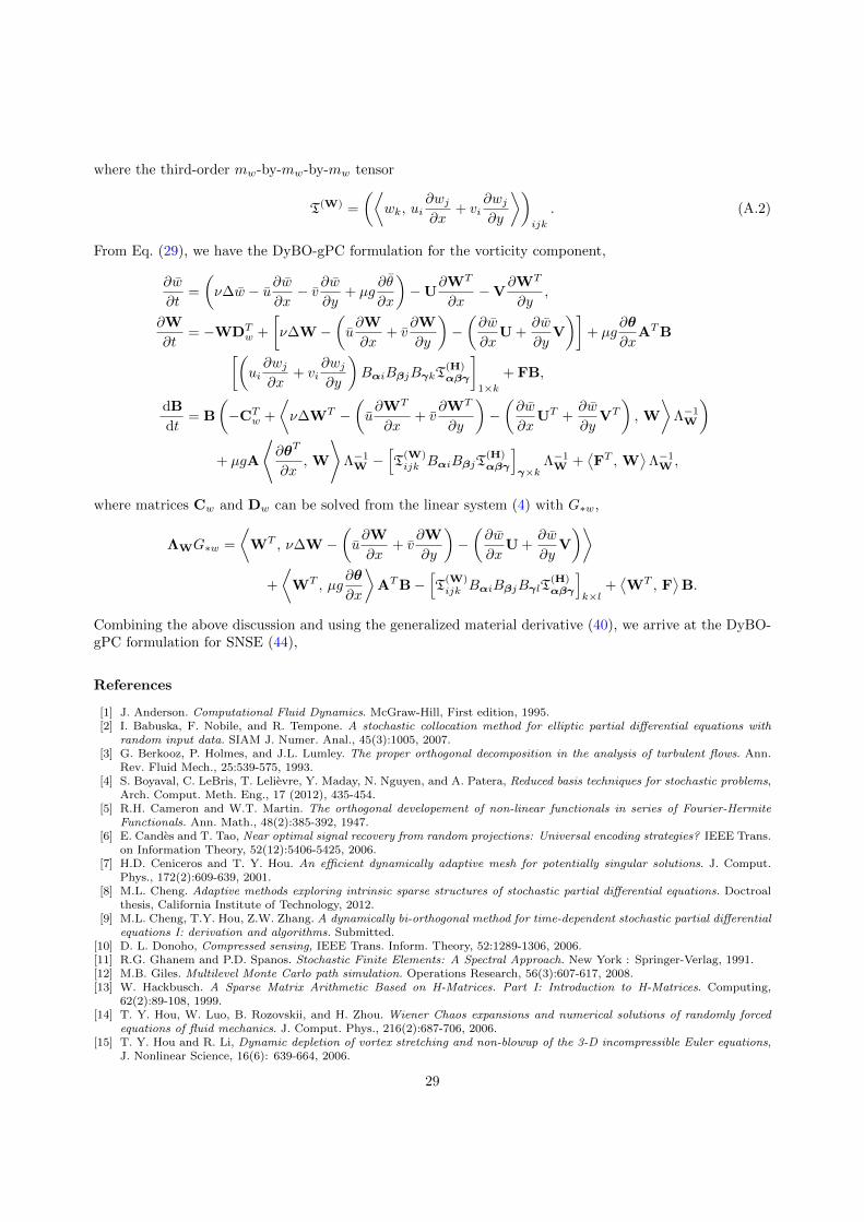
where the third-order mw-by-mw-by-mw tensor
T(W) =
(⟨wk, ui
∂wj∂x
+ vi∂wj∂y
⟩)ijk
. (A.2)
From Eq. (29), we have the DyBO-gPC formulation for the vorticity component,
∂w
∂t=
(ν∆w − u∂w
∂x− v ∂w
∂y+ µg
∂θ
∂x
)−U
∂WT
∂x−V
∂WT
∂y,
∂W
∂t= −WDT
w +
[ν∆W −
(u∂W
∂x+ v
∂W
∂y
)−(∂w
∂xU +
∂w
∂yV
)]+ µg
∂θ
∂xATB[(
ui∂wj∂x
+ vi∂wj∂y
)BαiBβjBγkT
(H)αβγ
]1×k
+ FB,
dB
dt= B
(−CT
w +
⟨ν∆WT −
(u∂WT
∂x+ v
∂WT
∂y
)−(∂w
∂xUT +
∂w
∂yVT
), W
⟩Λ−1W
)+ µgA
⟨∂θT
∂x, W
⟩Λ−1W −
[T
(W)ijk BαiBβjT
(H)αβγ
]γ×k
Λ−1W +
⟨FT , W
⟩Λ−1W ,
where matrices Cw and Dw can be solved from the linear system (4) with G∗w,
ΛWG∗w =
⟨WT , ν∆W −
(u∂W
∂x+ v
∂W
∂y
)−(∂w
∂xU +
∂w
∂yV
)⟩+
⟨WT , µg
∂θ
∂x
⟩ATB−
[T
(W)ijk BαiBβjBγlT
(H)αβγ
]k×l
+⟨WT , F
⟩B.
Combining the above discussion and using the generalized material derivative (40), we arrive at the DyBO-gPC formulation for SNSE (44),
References
[1] J. Anderson. Computational Fluid Dynamics. McGraw-Hill, First edition, 1995.[2] I. Babuska, F. Nobile, and R. Tempone. A stochastic collocation method for elliptic partial differential equations with
random input data. SIAM J. Numer. Anal., 45(3):1005, 2007.[3] G. Berkooz, P. Holmes, and J.L. Lumley. The proper orthogonal decomposition in the analysis of turbulent flows. Ann.
Rev. Fluid Mech., 25:539-575, 1993.[4] S. Boyaval, C. LeBris, T. Lelievre, Y. Maday, N. Nguyen, and A. Patera, Reduced basis techniques for stochastic problems,
Arch. Comput. Meth. Eng., 17 (2012), 435-454.[5] R.H. Cameron and W.T. Martin. The orthogonal developement of non-linear functionals in series of Fourier-Hermite
Functionals. Ann. Math., 48(2):385-392, 1947.[6] E. Candes and T. Tao, Near optimal signal recovery from random projections: Universal encoding strategies? IEEE Trans.
on Information Theory, 52(12):5406-5425, 2006.[7] H.D. Ceniceros and T. Y. Hou. An efficient dynamically adaptive mesh for potentially singular solutions. J. Comput.
Phys., 172(2):609-639, 2001.[8] M.L. Cheng. Adaptive methods exploring intrinsic sparse structures of stochastic partial differential equations. Doctroal
thesis, California Institute of Technology, 2012.[9] M.L. Cheng, T.Y. Hou, Z.W. Zhang. A dynamically bi-orthogonal method for time-dependent stochastic partial differential
equations I: derivation and algorithms. Submitted.[10] D. L. Donoho, Compressed sensing, IEEE Trans. Inform. Theory, 52:1289-1306, 2006.[11] R.G. Ghanem and P.D. Spanos. Stochastic Finite Elements: A Spectral Approach. New York : Springer-Verlag, 1991.[12] M.B. Giles. Multilevel Monte Carlo path simulation. Operations Research, 56(3):607-617, 2008.[13] W. Hackbusch. A Sparse Matrix Arithmetic Based on H-Matrices. Part I: Introduction to H-Matrices. Computing,
62(2):89-108, 1999.[14] T. Y. Hou, W. Luo, B. Rozovskii, and H. Zhou. Wiener Chaos expansions and numerical solutions of randomly forced
equations of fluid mechanics. J. Comput. Phys., 216(2):687-706, 2006.[15] T. Y. Hou and R. Li, Dynamic depletion of vortex stretching and non-blowup of the 3-D incompressible Euler equations,
J. Nonlinear Science, 16(6): 639-664, 2006.
29

[16] T. Y. Hou and R. Li, Computing nearly singular solutions using pseudo-spectral methods, J. Comput. Phys., 226:379-397,2007.
[17] T. Y. Hou and Z. Shi, Adaptive aata analysis via sparse time-frequency representation. Advances in Adaptive DataAnalysis, 3:1-28, 2011.
[18] T. Y. Hou and Z. Shi, Data-Driven Time-Frequency Analysis. Applied and Comput. Harmonic Anal., accepted, 2012.[19] K. Karhunen. Uber lineare Methoden in der Wahrscheinlichkeitsrechnung. Ann. Acad. Sci. Fennicae. Ser. A. I. Math.-Phys.
37:1-79, 1947.[20] O. Le Maitre. Uncertainty propagation using Wiener-Haar expansions. J. Comput. Phys., 197(1):28-57, 2004.[21] M. Loeve, Probability Theory. Vol. II, 4th ed. GTM. 46. Springer-Verlag. ISBN 0-387-90262-7.[22] W. Luo. Wiener chaos expansion and numerical solutions of stochastic partial differential equations. Ph.D. thesis, Cali-
fornia Institute of Technology, 2006.[23] W. Ma, M. Yu, J. Xin, and S. Osher. A convex model and L1 minimization for musical noise reduction in blind source
separation. Commun. Math Sci., 10(1):223-238, 2012.[24] Y. Maday, Reduced-basis method for the rapid and reliable solution of partial differential equations. In: Proceedings of
international conference of mathematicians, Madrid. European Mathematical Society, Zurich, 2006.[25] W.J. Morokoff and R.E. Caflisch. Quasi-sandom sequences and their discrepancies. SIAM J Sci. Comput., 15(6):1251-1279,
1994.[26] H. Niederreiter Random number generation and quasi-Monte Carlo methods. SIAM Publ., 1992.[27] G. Rozza, D. B. P Huynh, and A. T. Patera, Reduced basis approximation and a posteriori error estimation for affinely
parametrized elliptic coercive partial differential equations. Application to transport and continuum mechanics. ArchComput Methods Eng 15(3):229-275, 2008.
[28] T.P. Sapsis and P.F.J. Lermusiaux. Dynamically orthogonal field equations for continuous stochastic dynamical systems.Physica D, 238:2347-2360, 2009.
[29] T.P. Sapsis and P.F.J. Lermusiaux. Dynamical criteria for the evolution of the stochastic dimensionality in flows withuncertainty. Physica D, 241(1):60-76, 2012.
[30] D. Venturi. On proper orthogonal decomposition of randomly perturbed fields with applications to flow past a cylinder andnatural convection over a horizontal plate. J. Fluid Mech., 559:215-254, 2006.
[31] N. Wierner. The homogeneous chaos. Amer. J. Math., 60:897-936, 1938.[32] D. Xiu and G.E. Karniadakis. The Wiener-Askey polynomial chaos for stochastic differential equations. SIAM J. Sci.
Comput., 24(2):614-644, 2002.[33] D. Xiu and G.E. Karniadakis. Modeling uncertainty in flow simulations via generalized polynomial chaos. J. Comput.
Phys., 187(1):137-167, 2003.[34] M. Yu, W. Ma, J. Xin and S. Osher. Multi-channel L1 regularized convex speech enhancement model and fast computation
by the split Bregman method. IEEE Trans. Audio, Speech and Language Processing, 20(2):661-675, 2012.
30