Embed Size (px)
Citation preview

Kyoto University, Graduate School of Economics Discussion Paper Series
A Factor Pricing Model under Ambiguity
Katsutoshi Wakai
Discussion Paper No. E-17-012
Graduate School of Economics Kyoto University
Yoshida-Hommachi, Sakyo-ku Kyoto City, 606-8501, Japan
March, 2018

A Factor Pricing Model under Ambiguity�
Katsutoshi Wakaiy
March 13, 2018
Abstract
We derive a factor pricing model under the economy where the representative
agent�s preferences follow the smooth model of decision making under ambiguity as
proposed by Klibano¤, Marinacci, and Mukerji (2005). A newly derived factor is
called an ambiguity factor that captures a component of returns generated by ambigu-
ity aversion.
Keywords: Ambiguity aversion, asset pricing, factor pricing
JEL Classi�cation Numbers: D81, G11, G12
�I gratefully acknowledge the �nancial support from the Japanese government in the form of research
grant, Grant-in-Aid for Scienti�c Research (C) (26380235, 17K03622).
yGraduate School of Economics, Kyoto University, Yoshida-honmachi, Sakyo-ku, Kyoto 606-8501, Japan;
E-mail: [email protected]
1

1 Introduction
Conventionally, �nance theory deals with the situation where returns of assets are deter-
mined via objectively given probability distributions. This line of research produces empiri-
cally testable frameworks for cross-sectional returns, such as the capital asset pricing model
(CAPM) suggested by Lintner (1965), Mossin (1966), and Sharpe (1964) and the factor
pricing model suggested by Fama and French (1996) and many others. Recently, the theory
is extended to the situation where an investor does not know an objective distribution of
returns or at least he is unsure about how empirical frequency of data is generated. Such a
situation is called ambiguity, which is distinct from the risk the conventional �nance theory
has been studying.1
We aim to extend a factor pricing model to the case where investors face ambiguity. For-
mally, we approximate the pricing kernel derived under a smooth model of decision making
under ambiguity suggested by the Klibano¤, Marinacci, and Mukerji (2005). In their model,
the investor believes that there exist a number of possible regimes each of which speci�es
objective probability of state realization, but he is unsure which regime he faces. The in-
vestor behaves as an risk averse expected utility maximizer under each possible regime but
expresses an aversion to the ambiguity of a given regime. For this concern, the investor
forms a subjective prior over these possible regimes and behaves as to avoid the variability
of expected utility computed at each possible regime.
If the investor is ambiguity neutral, Klibano¤et al. (2005) reduces to a standard expected
utility, which with rational expectations assumption can produce a standard factor pricing
formula. In our approximation, an excess return corresponds to this component is called
a factor risk premium. What new in our factor pricing formula is an introduction of an
ambiguity factor, which account for the variation of returns due to ambiguity aversion. The
expected excess return is then shown to be a summation of two components, factor risk
1Knight (1921) is the �rst person who recognize this distinction.
2
premium and factor ambiguity premium. We identify the conditions on the representative
agent economy that derive this ambiguity-augumented version of a factor pricing formula. A
simple canonical example is also provided so that an economy that satis�es such conditions
are not empty.
As for the related literature, Ru¢ no (2014) and Wakai (2015) independently show that
the CAPM can be extended to the case where investors face ambiguity. Formally, they
adopt the robust mean-variance preferences suggested by Maccheroni, Marinacci, and Ru¢ no
(2013), which models an aversion to incomplete knowledge about possible economic regimes
the investor faces.2 The derived relation among equilibrium asset returns, called the robust
CAPM, di¤ers from the CAPM only in terms of coe¢ cient beta that determines the excess
return. This newly derived augumented-beta is shown to be a convex combination of risk
beta and ambiguity beta, the former of which is identical to the beta in the standard CAPM.
The new component, the ambiguity beta, measure the amount of ambiguity in asset returns
priced relative to the ambiguity in market returns.
In this paper, we show that the robust CAPM can be rewritten as a factor model with
one risk factor and one ambiguity factor, which is exactly identical to a version of our factor
pricing formula. However, the restriction on the factor ambiguity premium is di¤erent. In
the robust CAPM, the factor ambiguity premium must be less than the factor risk premium,
whereas in our model, the factor ambiguity premium can be larger than the factor risk
premium.
2 Setting
We consider a single-period portfolio choice problem. Let (;F ; P ) be a probability space.
At each state, a single perishable consumption good de�ned on R is available. There is a
2The robust mean-variance preferences are characterized as the approximation of Klibano¤, Marinacci,
and Mukerji�s (2005) smooth model of decision making under ambiguity.
3
single representative agent in this economy, who is endowed with the positive and bounded
consumption e measurable with respect to F . There are a �nite number K + 1 of assets
that pay a nonnegative amount of consumption good as a dividend. The payo¤s of the �rst
K assets are not deterministic, while the (K + 1)th asset is the risk-free asset that pays one
unit of consumption good. We denote by d = (d1; :::; dK+1) the vector of assets�dividends,
each element of which is a bounded random variable measurable with respect to F . All of
assets have net zero supply.
We model ambiguity as follows: The representative agent believes that there are a �-
nite number L of possible regimes in this economy and that he is unsure which regime he
faces. Each regime l speci�es the probability of state realization, denoted by an absolutely
continuous Ql with respect to P , and investor�s belief of possible regimes is expressed by
his subjective prior � de�ned over L regimes. Let (L;P(L); �) be a probability space that
describes the agent belief, where P(L) is the power set de�ned on L.
For a random variable x measurable with respect to F , we denote by EQ[x] a random
variable measurable with respect to P(L), where for each l, EQ[x jl ] is the expectation of
x under the probability measure Ql. We also denote by E�[a] the expectation of a random
variable a measurable with respect to P(L) under the probability measure �. Furthermore,
following Maccheroni et. all. (2013), we de�ne the probability measure bP on F , called thereduction of � on , by
bP (A) = �(1)Q1(A) + :::+ �(L)QL(A) for all A 2 F :Let E bP [x] be the expectation of a random variable x measurable with respect to F under
the reduction bP .We assume that the representative agent can trade assets without transaction cost and
can short and borrow without restrictions. Let c be a feasible consumption, which satis�es
the following budget constraints:
� � q = 0; (1)
4

and
c = e+ � � d; (2)
where � = (�1; :::; �K+1) 2 RK+1 is the vector of asset holdings and q = (q1; :::; qK+1) 2 RK+1+
is the vector of assets�prices.
The representative agent�s preferences follow a smooth model of decision making under
ambiguity as introduced by Klibano¤ et al. (2005)
V (c) = E� [v (EQ [u (c)])] ; (3)
where both v and u are strictly increasing and strictly concave on the respective domain.
The representative agent decides his asset holdings � so as to maximize the representation
(3). Appendix A shows that the equilibrium price qk satis�es
qk =E� [v
0 � EQ [m� dk]]
E� [v0 � EQ [m]]�1
qK+1
; (4)
where v0 is P(L)-measurable and m is F-measurable random variables that stand for
v0 � v0 (EQ [u (e)]) and m � u0 (e) . (5)
We also introduce a few more notations. Let Rk be the gross return of k-th risky asset,
and let Rf be the gross return of the risk-free asset. We denote by Cov� [a; b] the covariance
between P(L)-measurable a and b under �. A variance of P(L)-measurable a under �,
V ar� [a], is similarly de�ned. Furthermore, for random variables x and y measurable with
respect to F , let CovQ [x; y] be a random variable measurable with respect to P(L), where
for each l, CovQ[x; y jl ] is the covariance between x and y under Ql. Later, we also use
Cov bP [x; y] to denote the covariance between F-measurable x and y under bP . A variance ofF-measurable x under bP , V ar bP [x], is similarly de�ned. As commonly used, 1 denotes thevector of one de�ned on , whereas 1L denotes the vector of one de�ned on L.
Given the above notations, as shown in Appendix A, (4) is rewritten as follows:
E bP [Rk �Rf ] = �fE� [v0 � CovQ [m;Rk]] + Cov� [v0 � EQ [m] ; EQ [Rk]]g
E� [v0 � EQ [m]]: (6)
5

3 Factor Pricing under Ambiguity
3.1 Motivation
In empirical studies of asset returns, we often assume a factor pricing formula
EP [Rk �Rf ] =IXi=1
�k;iEP [RRFi �Rf ]; (7)
where a set of gross portfolio returns and the risk-free return, fRRF1 ; RRF2 ; :::; RRFI ; Rfg, is
assumed to be linearly independent. The model is based on the expected utility by imposing
a particular assumption on m, where the factor return RRFi captures the variation of m that
is relevant for asset pricing. Because risk aversion determines the variation of m, the factor
risk premium EP [RRFi �Rf ] represents a risk premium associated with factor returns.
In this paper, we intend to derive a similar decomposition of returns by introducing a
premium associated with ambiguity aversion. Intuitively, we want to have
EP [Rk �Rf ] = (factor ambiguity premium) + (factor risk premium),
where the latter has a form similar to that shown in (7). Because risk aversion and ambiguity
aversion interwind nonlinearly, it is not always possible to decompose returns exactly as
above. We later provide a canonical example in which the above decomposition holds, where
the part of returns associated with the variation of m is regarded as to risk premium and the
part of the returns associated with the variation of v0 is regarded as to ambiguity premium.
3.2 Risk Premium
For asset returns based on (4), we �rst want to identify the part of returns associated with
the variation of m. We follow the approach used for the expected utility model and derive a
version of a factor pricing formula by imposing a spanning condition on m. For this purpose,
6

notice that there exist a prior e� de�ned on (L;P(L)) so thatqk =
Ee� [EQ [m� dk]]Ee� [EQ [m]]�Rf ;
where e�(l) � v0 � �(l)E� [v0]
. Then an argument similar to Gollier (2011) shows that there exists
a prior eP de�ned on (;F) such that (4) is rewritten asqk =
E eP [m� dk]E eP [m]�Rf ; (8)
where eP (A) = e�(1)Q1(A) + :::+ e�(L)QL(A) for all A 2 F :Equation (8) is a common pricing formula derived under the expected utility with a subjective
prior eP .Now, for a �nite I � K, consider a set of gross portfolio returns and the risk-free return
fRRF1 ; RRF2 ; :::; RRFI ; Rfg, which is assumed to be linearly independent. We then impose
the following.
Assumption 1: (Spanning Condition on m)
(i) m = a0Rf +IXi=1
aiRRFi + �, where ai 6= 0 for any i 2 f1; :::; Ig :
(ii) E eP [��Rk] = 0 for all k.Assumption 1 is a well-known condition that leads to the following form of a factor pricing
model.
E eP [Rk �Rf ] =IXi=1
e�k;iE eP [RRFi �Rf ]; (9)
where e�k;i is obtained as a coe¢ cient of (RRFi �Rf ) by the regression of the excess return(Rk �Rf ) on excess factor returns (RRF1 �Rf ; :::; RRFI �Rf ) under eP .3
3Theoretically, these coe¢ cients must be identical to those obtained from the regression that includes the
constant term, where the coe¢ cient of the constant term turns out to be zero.
7
Equation (9) states that if we use eP , the excess returns should be written as a factorpricing model where the factor return RRFi captures the variation of m that is relevant for
asset pricing. However, the empirical factor pricing formula (7) is based on the objective
probability P . Thus, in the next subsection, we aim to identify the condition under which
a bias of the subjective prior eP relative to the objective probability P tells us an ambiguityrelated premium.
3.3 Alpha from Ambiguity Aversion
In this subsection, we want to identify the e¤ect of ambiguity. For this purpose, we introduce
an assumption that links the agent�s belief and the objective probability.
Assumption 2: (Rational Belief)
(i) bP = P .This assumption is a version of rational expectation hypothesis adopted to the smooth
model of decision making under ambiguity, and it corresponds to a similar assumption
adopted to the subjective expected utility model. Given Assumption 2, the agent has the re-
duction, that is the belief on state realization, which is consistent with the frequency of data.
The agent simply does not know how this frequency is generated so that he assumes regimes
that seemingly consistent with data. This assumption also contributes to the separation
of the ambiguity aversion from risk aversion because if the agent is ambiguity neutral, (4)
reduces to the pricing under the subjective expected utility model with rational expectations.
The following proposition shows that the regression constant captures a premium related
to ambiguity aversion (see Appendix B).
Proposition 1:
Suppose that Assumptions 1 and 2 hold. For each k, the gross return of asset k satis�es the
8

factor pricing formula
EP [Rk �Rf ] = �k +IXi=1
�k;iEP [RRFi �Rf ]; (10)
or
Rk �Rf = �k +IXi=1
�k;i (RRFi �Rf ) + "k; (11)
where for each i, �k;i is a regression coe¢ cient for RRFi �Rf . Furthermore, EP ["k] = 0 and
�k satis�es
�k = �E� [v
0 � EQ [m� "k]]E� [v0 � EQ [m]]
: (12)
Moreover, if the representative agent is ambiguity neutral, �k is zero.
For each i, we call EP [RRFi � Rf ] the factor risk premium. Note that �k;i in (10), which
is obtained as a coe¢ cient of (RRFi �Rf ) by the regression of the excess return (Rk �Rf )
on a set of returns (1; RRF1 �Rf ; :::; RRFI �Rf ) under P , need not be identical to the
regression coe¢ cient e�k;i shown in (9). Also note that we cannot eliminate the e¤ect ofambiguity aversion from the factor returns in (10) because ambiguity aversion in�uences the
levels of fq1; :::; qKg.
Proposition 1 shows that the regression constant �k captures a premium related to
ambiguity: If the agent is ambiguity neutral (that is, v is linear), �k is zero because
E� [EQ [m� "k]] = EP [m� "k] = 0. Indeed, under Assumption 2, we can show that for
a regression on any set of portfolio returns, �k needs to satisfy (12), which represents�1qK+1
times a price of the regression error. If this idiosyncratic variation is bene�cial to hedge risk
or ambiguity, it requires the negative premium, and vice versa. In fact, even for an ambiguity
neutral agent, �k can be nonzero for some regression. What Assumption 1 introduces is the
condition under which �k represents a premium contingent on the existence of ambiguity
aversion, once a factor regression is correctly speci�ed.
Note that equation (10) with a similar interpretation of �k holds under Gilboa and
Schmeidler�s (1989) multiple-priors model with an e¤ectively selected prior eP . The advantage9
of Klibano¤ et al. (2005) is that we can introduce Assumption 2, which enables us to derive
more elaborate interpretation of the regression constant �k, as shown in the next section.
For the following study, we also want to emphasize the relation between the regression
coe¢ cient �k and the residual "k.
Corollary 1:
Suppose that Assumptions 1 and 2 hold. Assume that is �nite, where the number of states
is less than or equal to K+1, that is, the asset market is complete. Moreover, let I = jj�1.
Then, generically, the gross return of asset k satis�es the factor pricing formula (10) with
�k = 0, so that in terms of the factor pricing formula, the economy with an ambiguity averse
agent is observationally equivalent to that with an ambiguity neutral agent.4
Corollary 1 states that if the asset market is complete and the factor returns completely span
any payo¤ vector, we cannot identify the e¤ect of ambiguity via the factor pricing formula.
This result shows that to identify the e¤ect of ambiguity, we need either an incomplete asset
market or a degenerate factor structure under which the number of factors is less than jj�1.
3.4 Ambiguity Premium
As Appendix C shows, �k can be decomposed into two parts, one is for a premium mainly
related to the ambiguity aversion, and the other is a premium generated by the interaction
between ambiguity aversion and risk aversion. However, there is no clear condition that
identi�es the latter e¤ect. Thus, we want to investigate a condition that makes �k, the joint
e¤ect of pure ambiguity and an interaction, have a factor pricing formula. We can at least
show that the following condition works.
Assumption 3:
4From (8), qk =EP [em�dk]EP [em]�Rf
, where em = md ePdP . Then em is generically spanned by I factors, so that (8)
holds under P . Moreover, for this case, "k = 0.
10
For each k, CovQ[m; "k jl ] = 0 for all l.
Assumption 3 states that the regression residual does not generate factor risk premium
at each regime l. This shuts a part of the connection between risk and ambiguity. Then, by
using well known statistical relation, we can rewrite �k as follows
�k = �E� [v
0 � EQ [m]� EQ ["k]]E� [v0 � EQ [m]]
: (13)
In this formula, the conditional connection betweenm and "k shown in EQ [m� "k] is broken
down to EQ [m]�EQ ["k]. Thus, by treating v0�EQ [m] as a ambiguity pricing kernel de�ned
on (L;P(L)), we can price a random variable EQ ["k]. For this part, we adopt a condition
similar to Assumption 1.
Assumption 4: (Spanning Condition on v0 � EQ [m])
(i) There exist J � K portfolios, each of whose returns is denoted by RAj , such that�EQ [RA1 ] ; :::; EQ [RAJ ] ; EQ
�Rf
�, becomes a set of linearly independent
vectors de�ne on the state space L.
(ii) v0 � EQ [m] = ea0EQ �Rf
�+
JXj=1
eajEQ �RAj�+ e�, where eaj 6= 0 for any j 2 f1; :::; Jg :(iii) E� [e�� EQ ["k]] = 0 for all k.For the next proposition, we de�ne the two more notations. Let k be given, where
1 � k � K. For each j satisfying 1 � j � J;
�Ek;j �Cov�
�EQ [Rk] ; EQ
�RAj
��V ar�
�EQ�RAj
�� ; (14)
and for each i and j satisfying 1 � i � I and 1 � j � J ,
�ERFi;j �Cov�
�EQ [RRFi ] ; EQ
�RAj
��V ar�
�EQ�RAj
�� : (15)
By de�nition, �Ek;j is a coe¢ cient ofEQ�RAj
�obtained by a regression ofEQ [Rk] on
�1L; EQ
�RAj
�under (L;P(L); �). Similarly, �ERFi;j is a coe¢ cient of EQ
�RAj
�obtained by a regression of
11
EQ [RRFi ] on�1L; EQ
�RAj
�under (L;P(L); �). Then the following proposition shows that
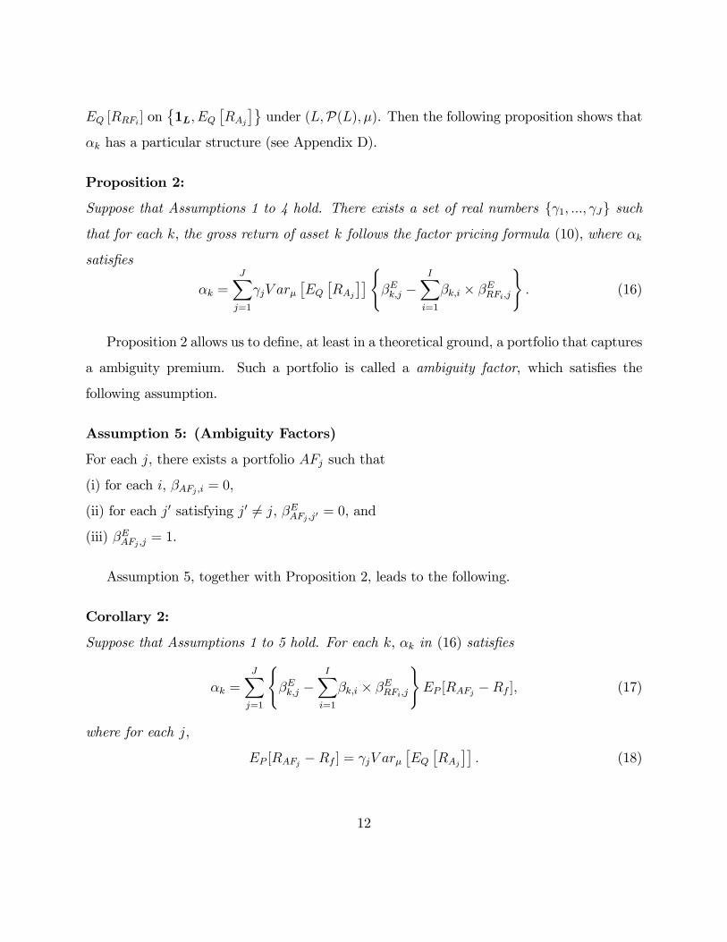
�k has a particular structure (see Appendix D).
Proposition 2:
Suppose that Assumptions 1 to 4 hold. There exists a set of real numbers f 1; :::; Jg such
that for each k, the gross return of asset k follows the factor pricing formula (10), where �k
satis�es
�k =JXj=1
jV ar��EQ�RAj
��(�Ek;j �
IXi=1
�k;i � �ERFi;j
): (16)
Proposition 2 allows us to de�ne, at least in a theoretical ground, a portfolio that captures
a ambiguity premium. Such a portfolio is called a ambiguity factor, which satis�es the
following assumption.
Assumption 5: (Ambiguity Factors)
For each j, there exists a portfolio AFj such that
(i) for each i, �AFj ;i = 0,
(ii) for each j0 satisfying j0 6= j, �EAFj ;j0 = 0, and
(iii) �EAFj ;j = 1.
Assumption 5, together with Proposition 2, leads to the following.
Corollary 2:
Suppose that Assumptions 1 to 5 hold. For each k, �k in (16) satis�es
�k =
JXj=1
(�Ek;j �
IXi=1
�k;i � �ERFi;j
)EP [RAFj �Rf ]; (17)
where for each j,
EP [RAFj �Rf ] = jV ar��EQ�RAj
��: (18)
12

Note that as (18) shows, for each j � J , the factor ambiguity premium EP [RAFj � Rf ] is
negative if j is negative. Also, in equation (17), �Ek;j represents the exposure to the factor
ambiguity premium from Rk itself. However, adjustment �IXi=1
�k;i � �ERFi;j is necessary
because �k is based on "k.
Corollary 2 allows us to rewrite (10) as follows
EP [Rk �Rf ] =JXj=1
(�Ek;j �
IXi=1
�k;i � �Ei;j
)EP [RAFj �Rf ] (19)
+IXi=1
�k;iEP [RRFi �Rf ]:
Also, we can rewrite (19) as follows
EP [Rk �Rf ] =JXj=1
�Ek;jEP [RAFj �Rf ] (20)
+IXi=1
�k;i
(EP [RRFi �Rf ]�
JXj=1
�Ei;jEP [RAFj �Rf ]):
The �rst line of (20) represents gross factor ambiguity premiums associate with Rk. In the
second line, for each i,
EP [RRFi �Rf ]�JXj=1
�ERFi;jEP [RAFj �Rf ]
is the ambiguity-adjusted factor risk premium or net factor risk premium.
The key di¤erence of the factor ambiguity premium from the factor risk premium is that
the coe¢ cient for the former e¤ect, either �Ek;j �IXi=1
�k;i � �ERFi;j or �Ek;j, is not obtained
as a coe¢ cient from the regression based on (19) or (20). This follows because the factor
ambiguity premium is based on the variations on (L;P(L); �), while the regression is based
on the variations on (;F ; P ). Thus, to identify the factor ambiguity premium, we need to
identify a coe¢ cient and an associated factor portfolio separately.
13
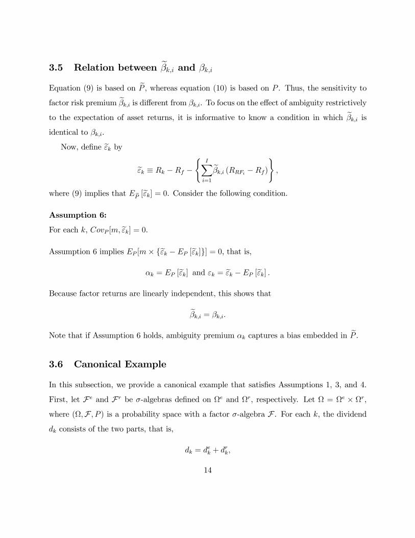
3.5 Relation between e�k;i and �k;iEquation (9) is based on eP , whereas equation (10) is based on P . Thus, the sensitivity tofactor risk premium e�k;i is di¤erent from �k;i. To focus on the e¤ect of ambiguity restrictivelyto the expectation of asset returns, it is informative to know a condition in which e�k;i isidentical to �k;i.
Now, de�ne e"k bye"k � Rk �Rf �( IX
i=1
e�k;i (RRFi �Rf ));
where (9) implies that E eP [e"k] = 0. Consider the following condition.Assumption 6:
For each k, CovP [m; e"k] = 0.Assumption 6 implies EP [m� fe"k � EP [e"k]g] = 0, that is,
�k = EP [e"k] and "k = e"k � EP [e"k] :Because factor returns are linearly independent, this shows that
e�k;i = �k;i:Note that if Assumption 6 holds, ambiguity premium �k captures a bias embedded in eP .3.6 Canonical Example
In this subsection, we provide a canonical example that satis�es Assumptions 1, 3, and 4.
First, let F e and F r be �-algebras de�ned on e and r, respectively. Let = e � r,
where (;F ; P ) is a probability space with a factor �-algebra F . For each k, the dividend
dk consists of the two parts, that is,
dk = dek + d
rk;
14

where dek is measurable only with respect to (e;F e) and drk is measurable only with respect
to (r;F r). Moreover, the endowment e is measurable only with respect to (e;F e). Because
of this construction, we call e the endowment space and r the idiosyncratic space. We
assume that the endowment space e is complete, that is, e is �nite with S states, where
there exists a set of lineally independent S assets whose dividends are measurable only
with respect to (e;F e). For convenience, let the �rst S � 1 risky assets be such linearly
independent assets without idiosyncratic dividends, which complete the endowment span
together with the risk-free asset. This construction guarantees Assumption 1, where the �rst
S � 1 risky assets become I risk factors. Furthermore, Corollary 1 is not applied because
a factor structure is degenerate, that is, there is no risk factor that spans the idiosyncratic
space.
Second, at each regime l, for each s; s0 2 e, Ql(:js) = Ql(:js0), that is, the conditional
probability is identical for all s 2 e. This means that the idiosyncratic dividend drk is
independently distributed from dek. By construction,
Rk = Rek +R
rk = (R
ek + EP [R
rk]) + (R
rk � EP [Rrk]);
where
Rek �dekqkand Rek �
drkqk:
Furthermore, (Rek + EP [Rrk]) is spanned by fR1; :::; RS�1; Rfg, and because the conditional
probability is identical for all s 2 e, EP [Rrk js ] = EP [Rrk] and EP [(R
rk � EP [Rrk]) js ] =
EP [(Rrk � EP [Rrk])] = 0 for all s 2 e. Thus, (Rrk�EP [Rrk]) is orthogonal to fR1; :::; RS�1; Rfg,
that is,
"k = Rrk � EP [Rrk]:
This implies Assumption 3 because m is measurable only with respect to (e;F e) and at
each regime l, for each s; s0 2 e, Ql(:js) = Ql(:js0).
Third, let L satisfy L � S = jej. Then, generically, fEQ [R1] ; :::; EQ [RS�1] ; Rfg spans
all variations de�ned on (L;P(L); �). Thus, Assumption 4 is generically satis�ed with e� = 0.15

Fourth, the above argument implies also that Assumption 6 holds, that is, e�k;i = �k;i forall k and all i.
4 Relation to the CAPM and Fama and French (1996)
For an application of Klibano¤ et al. (2005), we often consider the case of J = 2. For
example, Ju and Miao (2012) assumes that the agent perceives the two regimes, one of the
regimes is a booming regime and the other is a recession regime. They show by a simulation
study that Klibano¤ et al.�s (2005) model is consistent with many of regularities observed
in �nancial data. Moreover, Gallant, Jahan-Parvar, and Liu (2015) estimate Ju and Miao�s
(2012) model via the Bayesian method and show that �nancial data implies the high degree
of ambiguity aversion.
To derive a clear intuition about our model, we follow the above authors and focus on
the case of J = 2. The intuition gained here can be easily applied to the case of J > 2.
When J = 2, (19) becomes
EP [Rk �Rf ] =(�Ek;1 �
IXi=1
�k;i � �Ei;1
)EP [RAF1 �Rf ] +
IXi=1
�k;iEP [RRFi �Rf ]: (21)
Thus, a single ambiguity factor RAF1 captures the factor ambiguity premium. For an expo-
sitional purpose, we use RAF and �Ek in place of RAF1 and �Ek;1 in the following subsection.
4.1 Ambiguity-augumented CAPM
In this section, we derive an ambiguity-augumented version of the CAPM. Let RM be a gross
return of a market portfolio whose dividend is equal to e (equivalently, is proportional to
e). We assume that the market portfolio is tradable. Without loss of generality, let the �rst
risky asset be the market portfolio.
It is well known that the CAPM suggested by Lintner (1965), Mossin (1966), and Sharpe
16
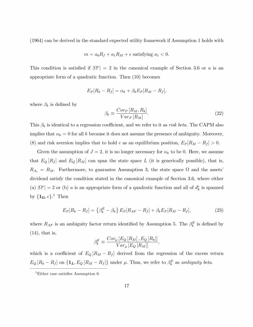
(1964) can be derived in the standard expected utility framework if Assumption 1 holds with
m = a0Rf + a1RM + � satisfying a1 < 0.
This condition is satis�ed if jej = 2 in the canonical example of Section 3.6 or u is an
appropriate form of a quadratic function. Then (10) becomes
EP [Rk �Rf ] = �k + �kEP [RM �Rf ];
where �k is de�ned by
�k �CovP [RM ; Rk]
V arP [RM ]: (22)
This �k is identical to a regression coe¢ cient, and we refer to it as risk beta. The CAPM also
implies that �k = 0 for all k because it does not assume the presence of ambiguity. Moreover,
(8) and risk aversion implies that to hold e as an equilibrium position, EP [RM �Rf ] > 0.
Given the assumption of J = 2, it is no longer necessary for �k to be 0. Here, we assume
that EQ [Rf ] and EQ [RM ] can span the state space L (it is generically possible), that is,
RA1 = RM . Furthermore, to guarantee Assumption 3, the state space and the assets�
dividend satisfy the condition stated in the canonical example of Section 3.6, where either
(a) jej = 2 or (b) u is an appropriate form of a quadratic function and all of dek is spanned
by f1; eg.5 Then
EP [Rk �Rf ] =��Ek � �k
EP [RAF �Rf ] + �kEP [RM �Rf ]; (23)
where RAF is an ambiguity factor return identi�ed by Assumption 5. The �Ek is de�ned by
(14), that is,
�Ek �Cov� [EQ [RM ] ; EQ [Rk]]
V ar� [EQ [RM ]];
which is a coe¢ cient of EQ [RM �Rf ] derived from the regression of the excess return
EQ [Rk �Rf ] on f1L; EQ [RM �Rf ]g under �. Thus, we refer to �Ek as ambiguity beta.
5Either case satis�es Assumption 6.
17

We �rst investigate a sign of the factor ambiguity premium EP [RAF � Rf ]. Let l =
1 be a booming regime and let l = 2 be a recession regime, where EQ [u (e) jl = 1] >
EQ [u (e) jl = 2]. This implies that v0 (EQ [u (e) jl = 1]) < v0 (EQ [u (e) jl = 2]). On the
other hand, the assumption of the model does not provide an enough information to in-
duce EQ [m jl = 1] < EQ [m jl = 2] or EQ [RM jl = 1] > EQ [RM jl = 2]. However, be-
cause RM is perfectly correlated with e, it is likely that EQ [m jl = 1] < EQ [m jl = 2] and
EQ [RM jl = 1] > EQ [RM jl = 2]. If so, as Appendix D show, 1 > 0. Thus, EQ [RM ] does
not provides a hedge against ambiguity so that an associated factor ambiguity premium
EP [RAF � Rf ] must be positive. Moreover, the factor ambiguity premium EP [RAF � Rf ]
tends to increase as the agent becomes more ambiguity averse. This happens because 1
tends to increase as the volatility of v0 increases.
We want to emphasize a few important aspects of (23). First, the interpretation of
risk beta �k is analogous to that for the CAPM beta, that is, only the risk contributing to
market volatility is priced. Thus, a positively contributed asset earns a positive excess return
because it bears market risk, whereas a negatively contributed asset earns a negative excess
return because it provides a hedge against market risk. Second, as for the interpretation
of �Ek , V ar� [EQ[RM ]] measures market ambiguity, and Cov� [EQ[Rk]; EQ[RM ]] measures
the contribution of asset k�s expected return to market ambiguity. Thus, �Ek de�nes the
compensation scheme for ambiguity, which is analogous to that for market risk. Third,
the coe¢ cient of the ambiguity factor RAF is not identical to the coe¢ cient obtained by
the multivariable regression of Rk � Rf on f1, RAF �Rf , RM �Rfg under P . It is a
di¤erence between ambiguity beta and risk beta. Therefore, only the net ambiguity exposure
is compensated by the ambiguity premium.
To emphasize the e¤ect of ambiguity aversion, (23) can be rewritten as
EP [Rk �Rf ] = �Ek EP [RAF �Rf ] + �k fEP [RM �Rf ]� EP [RAF �Rf ]g :
The �rst term indicates the gross factor ambiguity premium associated with Rk, whereas the
18

second term indicates the net factor risk premium associated with Rk. Because �M = �EM =
1, the latter is an incremental risk premium embedded in EP [RM �Rf ] after subtracting the
ambiguity e¤ect. To judge the relative importance of risk aversion to ambiguity aversion, it
is informative to know the sign of the net factor risk premium. However, the theory does not
provide enough information to conclude whether EP [RM �Rf ] is larger than EP [RAF �Rf ].
4.2 Ambiguity-augumented Fama-French Three Factor Model
Many researchers have proposed factor models, but for expositional purpose, we focus on
the model proposed by Fama and French (1996), referred to as the Fama-French three factor
model(changed on 9/21/17). The three factor returns consist of a return of a broad
stock market index portfolio, denoted by RM , a return of a portfolio composed of �rms with
small BP ratios minus �rms with large BP ratios, denoted by RHL, a return of a portfolio
composed of �rms with small capitalization minus �rms with large capitalization, denoted
by RSB. Each of risk factor returns have been shown to have a positive excess returns. For
the following study, we assume that RRF1 = RM and RA1 = RM . As shown in the above,
because RM is strongly correlated with e, the factor ambiguity premium EP [RAF � Rf ] is
likely to be positive.
We assume that Assumption 1 is satis�ed with the three factors de�ned above. Moreover,
to guarantee Assumption 3, the state space and the assets�dividend satisfy the condition
stated in the canonical example of Section 3.6, where either (a) jej = 4 or (b) all of dek
is spanned by f1; RM ; RHL; RSBg.6 If we take the factor risk premium as a basis, (21)
becomes
EP [Rk �Rf ] =��Ek � �k;1 � �k;2 � �EHL � �k;3 � �ESB
EP [RAF �Rf ]
+ �k;1EP [RM �Rf ] + �k;2EP [RHL �Rf ] + �k;3EP [RSB �Rf ]:
6Either case satis�es Assumption 6.
19

where �EHL = �EHL;1 and �
ESB = �
ESB;1. The coe¢ cient of the ambiguity factor is adjusted to
capture the factor ambiguity premium net of the risk e¤ect. On the other hand, if we take
the factor ambiguity premium as a basis, (21) can be rewritten as
EP [Rk �Rf ] = �Ek EP [RAF �Rf ]
+ �k;1 fEP [RM �Rf ]� EP [RAF �Rf ]g
+ �k;2�EP [RHL �Rf ]� �EHLEP [RAF �Rf ]
+ �k;3
�EP [RSB �Rf ]� �ESBEP [RAF �Rf ]
:
Here, to compute each of the net factor risk premium, we need to subtract the return associ-
ated with the ambiguity e¤ect, which must re�ect the correlation with the ambiguity factor,
that is, �EHL or �ESB. Again, to judge the relative importance of risk aversion to ambiguity
aversion, it is informative to know the sign of the net factor risk premium. However, the
theory does not provide enough information.
5 Relation to Maccheroni et al. (2013)
We have elicited a part of asset returns associated with ambiguity aversion by adopting a
linear approximation to a pricing kernel. In this section, we want to investigate a relation
of our results to asset pricing implications derived from another type of approximation of
Klibano¤ et al. (2005) proposed by Maccheroni et al. (2013).
First, we assume that the asset markets are complete, where is �nite and qs is the price
of the Arrow-Debreu asset for state s.7 Let W be the value of the endowment de�ned by
W �jjXs=1
es � qs;
where W is understood as a function of an endowment and state prices. Let w denote the
K-dimensional vector of portfolio weights on the K risky assets. Then, the return of the
7Alternatively, we can weaken this assumption by making e tradable.
20
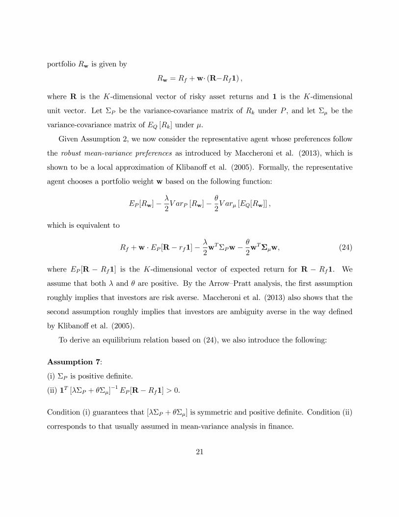
portfolio Rw is given by
Rw = Rf +w� (R�Rf1) ;
where R is the K-dimensional vector of risky asset returns and 1 is the K-dimensional
unit vector. Let �P be the variance-covariance matrix of Rk under P , and let �� be the
variance-covariance matrix of EQ [Rk] under �.
Given Assumption 2, we now consider the representative agent whose preferences follow
the robust mean-variance preferences as introduced by Maccheroni et al. (2013), which is
shown to be a local approximation of Klibano¤ et al. (2005). Formally, the representative
agent chooses a portfolio weight w based on the following function:
EP [Rw]��
2V arP [Rw]�
�
2V ar� [EQ[Rw]] ;
which is equivalent to
Rf +w � EP [R� rf1]��
2wT�Pw �
�
2wT��w; (24)
where EP [R � Rf1] is the K-dimensional vector of expected return for R � Rf1. We
assume that both � and � are positive. By the Arrow�Pratt analysis, the �rst assumption
roughly implies that investors are risk averse. Maccheroni et al. (2013) also shows that the
second assumption roughly implies that investors are ambiguity averse in the way de�ned
by Klibano¤ et al. (2005).
To derive an equilibrium relation based on (24), we also introduce the following:
Assumption 7:
(i) �P is positive de�nite.
(ii) 1T [��P + ���]�1EP [R�Rf1] > 0.
Condition (i) guarantees that [��P + ���] is symmetric and positive de�nite. Condition (ii)
corresponds to that usually assumed in mean-variance analysis in �nance.
21
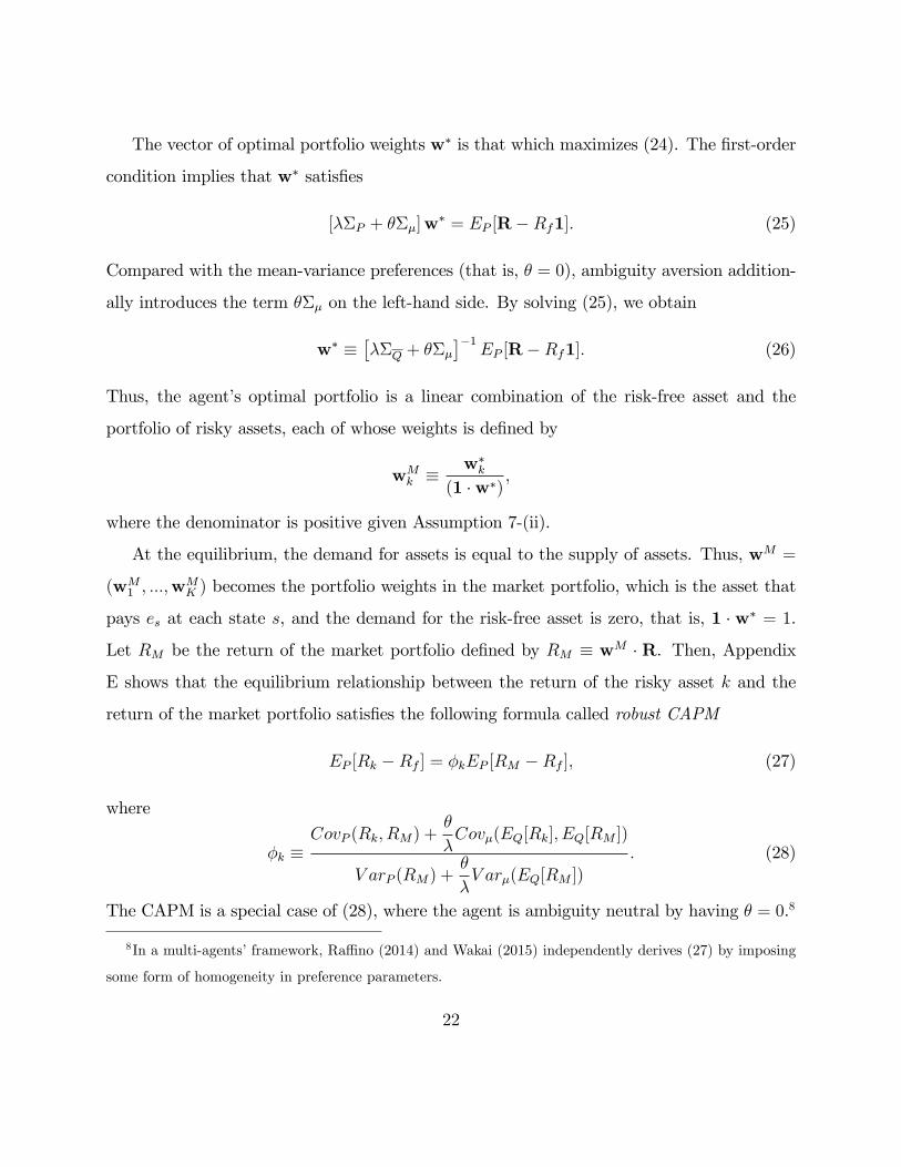
The vector of optimal portfolio weights w� is that which maximizes (24). The �rst-order
condition implies that w� satis�es
[��P + ���]w� = EP [R�Rf1]: (25)
Compared with the mean-variance preferences (that is, � = 0), ambiguity aversion addition-
ally introduces the term ��� on the left-hand side. By solving (25), we obtain
w� ����Q + ���
��1EP [R�Rf1]: (26)
Thus, the agent�s optimal portfolio is a linear combination of the risk-free asset and the
portfolio of risky assets, each of whose weights is de�ned by
wMk � w�
k
(1 �w�);
where the denominator is positive given Assumption 7-(ii).
At the equilibrium, the demand for assets is equal to the supply of assets. Thus, wM =
(wM1 ; :::;w
MK ) becomes the portfolio weights in the market portfolio, which is the asset that
pays es at each state s, and the demand for the risk-free asset is zero, that is, 1 � w� = 1.
Let RM be the return of the market portfolio de�ned by RM � wM � R. Then, Appendix
E shows that the equilibrium relationship between the return of the risky asset k and the
return of the market portfolio satis�es the following formula called robust CAPM
EP [Rk �Rf ] = �kEP [RM �Rf ]; (27)
where
�k �CovP (Rk; RM) +
�
�Cov�(EQ[Rk]; EQ[RM ])
V arP (RM) +�
�V ar�(EQ[RM ])
: (28)
The CAPM is a special case of (28), where the agent is ambiguity neutral by having � = 0.8
8In a multi-agents�framework, Ra¢ no (2014) and Wakai (2015) independently derives (27) by imposing
some form of homogeneity in preference parameters.
22
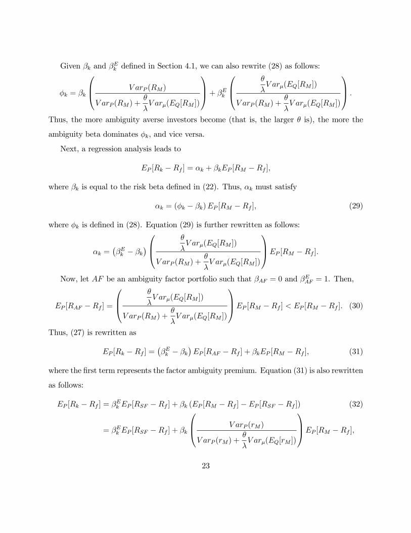
Given �k and �Ek de�ned in Section 4.1, we can also rewrite (28) as follows:
�k = �k
0B@ V arP (RM)
V arP (RM) +�
�V ar�(EQ[RM ])
1CA+ �Ek0B@ �
�V ar�(EQ[RM ])
V arP (RM) +�
�V ar�(EQ[RM ])
1CA :Thus, the more ambiguity averse investors become (that is, the larger � is), the more the
ambiguity beta dominates �k, and vice versa.
Next, a regression analysis leads to
EP [Rk �Rf ] = �k + �kEP [RM �Rf ];
where �k is equal to the risk beta de�ned in (22). Thus, �k must satisfy
�k = (�k � �k)EP [RM �Rf ]; (29)
where �k is de�ned in (28). Equation (29) is further rewritten as follows:
�k =��Ek � �k
�0B@ �
�V ar�(EQ[RM ])
V arP (RM) +�
�V ar�(EQ[RM ])
1CAEP [RM �Rf ]:Now, let AF be an ambiguity factor portfolio such that �AF = 0 and �EAF = 1. Then,
EP [RAF �Rf ] =
0B@ �
�V ar�(EQ[RM ])
V arP (RM) +�
�V ar�(EQ[RM ])
1CAEP [RM �Rf ] < EP [RM �Rf ]: (30)Thus, (27) is rewritten as
EP [Rk �Rf ] =��Ek � �k
�EP [RAF �Rf ] + �kEP [RM �Rf ]; (31)
where the �rst term represents the factor ambiguity premium. Equation (31) is also rewritten
as follows:
EP [Rk �Rf ] = �Ek EP [RSF �Rf ] + �k (EP [RM �Rf ]� EP [RSF �Rf ]) (32)
= �Ek EP [RSF �Rf ] + �k
0B@ V arP (rM)
V arP (rM) +�
�V ar�(EQ[rM ])
1CAEP [RM �Rf ];23
where in (32), (EP [RM �Rf ]� EP [RSF �Rf ]) represents the ambiguity-adjusted factor risk
premium.
Now, we want to compare the robust CAPM (that is, (31)) with the ambiguity-augumented
CAPM (that is, (23)), where for the latter model, u is assumed to be quadratic and the state
space and dividends satisfy the conditions stated in Section 4.1. First, the robust CAMP
holds even for the case of L 6= 2, but the ambiguity-augumented CAPM does not hold in
general if L 6= 2. Thus, for the robust mean-variance preferences, the equilibrium forces the
asset returns to have the factor ambiguity premium represented only by the �rst term of
(31). Second, in (31), the factor ambiguity premium is less than the factor risk premium
because of (30), whereas in (23), the factor ambiguity premium may be larger than the factor
risk premium.
24

Appendix A: The Derivation of Equations (4) and (6)
The investor maximizes (3) with the constraints (1) and (2), where the constraint (2) is
automatically satis�ed. By the �rst order condition with respect to �k leads to
E� [v0 (EQ [u (e+ � � d)])� EQ [u0 (e+ � � d)� dk]] = �qk; (33)
where � is the Lagrange multiplier corresponding to the constraint (1). In particular, at the
equilibrium, (33) implies that the equilibrium price qk must satisfy
E� [v0 (EQ [u (e)])� EQ [u0 (e)� dk]] = E� [v0 � EQ [m� dk]] = �qk: (34)
For the risk-free asset,
E� [v0 (EQ [u (e)])� EQ [u0 (e)]] = E� [v0 � EQ [m]] = �qK+1: (35)
Thus, (34) and (35) imply that at the equilibrium,
qk =E� [v
0 � EQ [m� dk]]
E� [v0 � EQ [m]]�1
qK+1
; (36)
which is (4).
By applying the standard statistical relation, (36) leads to
1 =fE� [v0 � CovQ [m;Rk]] + E� [v0 � EQ [m]EQ [Rk]]g
E� [v0 � EQ [m]]�Rf:
The second term of the numerator in the right-hand side is rewritten as
E� [v0 � EQ [m]EQ [Rk]] = Cov� [v0 � EQ [m] ; EQ [Rk]] + E� [v0 � EQ [m]]E� [EQ [Rk]] :
Thus, the above two equations imply
E bP [Rk �Rf ] = �fE� [v0 � CovQ [m;Rk]] + Cov� [v0 � EQ [m] ; EQ [Rk]]g
E� [v0 � EQ [m]]: (37)
which is (6). �
25

Appendix B: The Proof of Proposition 1
Given (37), by Assumptions 1 and 2, for each portfolio return RRFi
EP [RRFi �Rf ] (38)
=� fE� [v0 � CovQ [m;RRFi ]] + Cov� [v0 � EQ [m] ; EQ [RRFi ]]g
E� [v0 � EQ [m]]:
Now, we de�ne the following regression
EP [Rk �Rf ] = �k +IXi=1
�k;iEP [RRFi �Rf ]; (39)
or
Rk �Rf = �k +IXi=1
�k;i (RRFi �Rf ) + "k; (40)
where EP ["k] = 0. By applying (40) to (37), Assumptions 1 and 2 and (38) imply that
EP [Rk �Rf ] = b�k + IXi=1
�k;iEP [RRFi �Rf ]; (41)
where b�k = �fE� [v0 � CovQ [m; "k]] + Cov� [v0 � EQ [m] ; EQ ["k]]gE� [v0 � EQ [m]]
:
By comparing (39) and (41),
�k = b�k = �fE� [v0 � CovQ [m; "k]] + Cov� [v0 � EQ [m] ; EQ ["k]]gE� [v0 � EQ [m]]
: (42)
The �rst term of the numerator of the right-hand side becomes
E� [v0 � CovQ [m; "k]] = E� [v0 � EQ [m� "k]]� E� [v0 � EQ [m]EQ ["k]] ;
and the second term of the numerator of the right-hand side becomes
Cov� [v0 � EQ [m] ; EQ ["k]] = E� [v0 � EQ [m]EQ ["k]]� E� [v0 � EQ [m]]E� [EQ ["k]] ;
where the last term is zero because E� [EQ ["k]] = 0. Given the above two equations, (42) is
rewritten as
�k = �E� [v
0 � EQ [m� "k]]E� [v0 � EQ [m]]
;
which completes the proof. �
26

Appendix C:
Consider the situation where the agent is risk neutral and ambiguity neutral. Then, an
expected return of any asset is equal to the risk-free rate. Treating this case as a benchmark,
consider the situation where the agent is risk neutral. Then equation (10) becomes
EP [Rk �Rf ] = �k;
where �k satis�es equation (12) and it is zero if the agent is ambiguity neutral. Risk neutrality
also implies that
�k = �E� [v
0 � EQ [m� "k]]E� [v0 � EQ [m]]
= �E� [v0 � EP [m]� EQ ["k]]E� [v0 � EQ [m]]
(43)
because m is constant. The key here is that the variation of m is absent because of EP [m].
If we replace EP [m] in (43) with EQ [m], it generates an interaction between risk aversion
and ambiguity aversion because EQ [m] becomes nonconstant as soon as the agent becomes
risk averse. Thus, by using EP [m], we can isolate the e¤ect of ambiguity aversion that is
independent of risk aversion.
Following the above argument, we decompose the regression constant �k into two parts
as follows
�k = Ak +Bk;
where
Ak � �E� [v
0 � EP [m]� EQ ["k]]E� [v0 � EQ [m]]
(44)
and
Bk � �E� [v
0 � fEQ [m� "k]� EP [m]� EQ ["k]g]E� [v0 � EQ [m]]
: (45)
By comparing (44) and (45), we call Ak a pure ambiguity premium, which is a portion of
returns remained after the e¤ect of risk aversion is subtracted. Given this interpretation
of Ak, Bk represents an interaction e¤ect between risk aversion and ambiguity aversion. It
27

is easy to see that both Ak and Bk are zero if the agent is ambiguity neutral. Note that
technically speaking, risk aversion determines EP [m] so that we cannot isolate the exact
e¤ect of ambiguity aversion from the e¤ect of risk aversion.
Appendix D: The Proof of Proposition 2
By Assumption 4, (13) is rewritten as
�k = E�
"( 0EQ
�Rf
�+
JXj=1
jEQ�RAj
�)EQ ["k]
#; (46)
where 0 � �ea0
E� [v0 � EQ [m]]and j � �
eajE� [v0 � EQ [m]]
for each j.
We further evaluate (46) by
�k = E�
"( 0EQ
�Rf
�+
JXj=1
jEQ�RAj
�)EQ ["k]
#
=JXj=1
jE��EQ�RAj
�� EQ ["k]
�=
JXj=1
j�Cov�
�EQ�RAj
�; EQ ["k]
�+ E�
�EQ�RAj
��E� [EQ ["k]]
=
JXj=1
jCov��EQ�RAj
�; EQ ["k]
�:
By de�nition of "k, for each j,
jCov��EQ�RAj
�; EQ ["k]
�= jCov�
"EQ�RAj
�; EQ
"Rk �Rf � �k �
IXi=1
�k;i (RRFi �Rf )##
= j
(Cov�
�EQ�RAj
�; EQ [Rk]
��
IXi=1
�k;iCov��EQ�RAj
�; EQ [RRFi ]
�)
= jV ar��EQ�RAj
��(�Ek;j �
IXi=1
�k;i � �ERFi;j
):
28

Thus,
�k =
JXj=1
jV ar��EQ�RAj
��(�Ek;j �
IXi=1
�k;i � �ERFi;j
); (47)
as desired. �
Appendix E:
Multiplying (wM)T to (26) leads to
(wM)T [��P + ���]w� = EP [RM �Rf ];
which is equivalent to
(1 �w�)(wM)T [��P + ���]wM = EP [RM �Rf ]: (48)
(48) is positive because [��P + ���] is positive de�nite and (1 �w�) > 0.
Similarly, multiplying w(k)T to (26) leads to
w(k)T [��P + ���]w� = EP [Rk �Rf ]; (49)
where w(k) is a K-dimensional vector of asset weights that assigns one for asset k and zero
for others. Then, (49) is rewritten as
(1 �w�)w(k)T [��P + ���]wM = EP [Rk �Rf ]: (50)
Dividing (50) by (48) produces the following formula
EP [Rk �Rf ] = �kEP [RM �Rf ];
where
�k �w(k)T [��P + ���]w
M
(wM)T [��P + ���]wM=CovP (Rk; RM) +
�
�Cov�(EQ[Rk]; EQ[RM ])
V arP (RM) +�
�V ar�(EQ[RM ])
;
as desired. �
29
References
1. Fama, E., and K. French (1996): �Multifactor Explanations of Asset Pricing Anom-
alies,�Journal of Finance, Vol.51, pp.55-84.
2. Gallant, R., M. Jahan-Parvar, and H. Liu (2015): �Measuring Ambiguity Aversion,�
Finance and Economics Discussion Series, Division of Research & Statistics and Mon-
etary A¤airs, Federal Reserve Board Washington, D.C.
3. Gilboa, I., and D. Schmeidler (1989): �Maxmin Expected Utility with Nonunique
Prior,�Journal of Mathematical Economics, Vol.18, pp.141-153.
4. Gollier, Christian (2011): �Portfolio Choices and Asset Prices: The Comparative Sta-
tics of Ambiguity Aversion,�Review of Economic Studies, Vol.78, pp.1329-1344.
5. Ju, N., and J. Miao (2012): �Ambiguity, Learning, and Asset Returns,�Econometrica,
Vol.80, pp.559-591.
6. Klibano¤, P., M. Marinacci, and S. Mukerji (2005): �A Smooth Model of Decision
Making under Ambiguity,�Econometrica, Vol.73, pp.1849-1892.
7. Knight, F. (1921): Risk, Uncertainty and Pro�t, Houghton Mi in, Boston.
8. Lintner, J. (1965): �The Valuation of Risk Assets and the Selection of Risky Invest-
ments in Stock Portfolios and Capital Markets,�Review of Economics and Statistics,
Vol.47, pp.13-37.
9. Maccheroni, F., M. Marinacci, and D. Ru¢ no (2013): �Alpha as Ambiguity: Robust
Mean-Variance Portfolio Analysis,�Econometrica, Vol.81, pp.1075-1113.
10. Mossin, J. (1966): �Equilibrium in a Capital Asset Market,� Econmetrica, Vol.35,
pp.768-783
30
11. Ru¢ no, D. (2014): �A Robust Capital Asset Pricing Model,�Finance and Economics
Discussion Series, Division of Research & Statistics and Monetary A¤airs, Federal
Reserve Board Washington, D.C.
12. Sharpe, W. (1964): �Capital Asset Pricing: A Theory of Capital Market Equilibrium
under Conditions of Risk,�Journal of Finance, Vol.19, pp.425-442.
13. Wakai, K. (2015): �Equilibrium Alpha in Asset Pricing under Ambiguity Averse Econ-
omy,�Graduate School of Economics Discussion Paper Series E-15-010, Kyoto Univer-
sity.
31