Computers and Mathematics with Applications ( ) –

Contents lists available at ScienceDirect

Computers and Mathematics with Applications

journal homepage: www.elsevier.com/locate/camwa

A fast and stable algorithm for downdating the singular valuedecomposition

Jieyuan Zhang a,c, Shengguo Li b,∗, Lizhi Cheng a,c, Xiangke Liao b,Guangquan Cheng d

a College of Science, National University of Defense Technology, Changsha 410073, Chinab College of Computer Science, National University of Defense Technology, Changsha 410073, Chinac The State Key Laboratory for High Performance Computation, National University of Defense Technology, Changsha 410073, Chinad Science and Technology on Information Systems Engineering Laboratory, National University of Defense Technology,Changsha 410073, China

a r t i c l e i n f o

Article history:Received 31 January 2014Received in revised form 18 August 2014Accepted 13 September 2014Available online xxxx

Keywords:Downdating SVDHSS matricesCauchy-like matricesNumerical stability

a b s t r a c t

In this paper, we modify a classical downdating SVD algorithm and reduce its complexitysignificantly. We use a structured low-rank approximation algorithm to compute an hier-archically semiseparable (HSS) matrix approximation to the eigenvector matrix of a diag-onal matrix plus rank-one modification. The complexity of our downdating algorithm isanalyzed. We further show that the structured low-rank approximation algorithm is back-ward stable. Numerous experiments have been done to show the efficiency of our algo-rithm. For some matrices with large dimensions, our algorithm can be much faster thanthat using plain matrix–matrix multiplication routine in Intel MKL in both sequential andparallel cases.

© 2014 Elsevier Ltd. All rights reserved.

1. Introduction

Let A be anM × N real matrix,M > N , and assume that its SVD is defined as

A = UΣV T=U1 U2

Σ10

V T

= U1Σ1V T , (1)

where U =U1 U2

∈ RM×M and V ∈ RN×N are orthogonal matrices, U1 ∈ RM×N , and Σ1 ∈ RN×N is a diagonal matrix,

whose diagonal entries are the singular values of A. In this paper, we propose a fast algorithm to compute the SVD of A′

satisfying

A =

A′

aT

, (2)

where aT is the bottom row of A. Note that the case of deleting a column of A can be considered similarly.

∗ Corresponding author. Tel.: +86 13687340094.E-mail address: nudtlsg@nudt.edu.cn (S. Li).

http://dx.doi.org/10.1016/j.camwa.2014.09.0080898-1221/© 2014 Elsevier Ltd. All rights reserved.

2 J. Zhang et al. / Computers and Mathematics with Applications ( ) –

Computing the SVD of A′ is well-known as the downdating SVD problem [1], which has been widely applied in signalprocessing, image analysis and least square problems (see [2–5] formore details).Whenusing Latent Semantic Indexing (LSI)for information retrieval, some outdated terms and/or documents can be removed from the term-by-document matrix [6],which is also reduced to the downdating SVD problem.

Most algorithms for downdating SVD (see [1,3]) are expensive, costing O(N3) flops. For simplicity of analysis, we assumethatM and N are in the same order,M = O(N). In this paper, we show that the complexity of downdating SVD problem (2)can be reduced to O(N2r) flops,

A′= U ′Σ ′V ′T

=U ′

1 U ′

2

Σ ′

10

V ′T

= U ′

1Σ′

1V′T , (3)

where r is a moderate constant (see Section 3.2 for details), and U ′

1 ∈ R(M−1)×N . The technique used in this paper is similarto that in [7,8]. The main observation is that some intermediate matrices appeared in the algorithm in [1] are Cauchy-like matrices and have off-diagonal low-rank property, see Eqs. (7) and (8). We use hierarchically semiseparable (HSS)matrices [9–11] to approximate thesematrices, and then use fast HSSmatrix–matrixmultiplication algorithm [12] to updatethe singular vectors. Note that the updating SVD problem in [3,13] can be accelerated similarly.

To fully take advantage of these two properties, a structured low-rank approximation method is proposed for Cauchy-like matrices in [7,8], which is called SRRSC (structured rank-revealing Schur complement factorization). SRRSC only workson several vectors, therefore itsmemory cost is linearO(N). The complexity of using SRRSC to construct HSS approximationsis analyzed in Section 4.2, which is shown to be O(N2r), where N is the dimension of the matrix and r is a modest constantas above. In Section 4.3, the rounding error analysis of SRRSC is included, which shows that SRRSC is backward stable.

Numerous experiments have been done in Section 5 to show the efficiency of our algorithm. Since both the HSS construc-tion algorithm and HSS matrix–matrix multiplication algorithm are good for parallel, we further implement the proposeddowndating SVD algorithm by using OpenMP on the shared memory multicore platform. For matrices with large dimen-sions, the proposed downdating algorithm can be 3x–5x faster than that using plain matrix–matrix multiplication routinein Intel MKL in the serial and parallel cases.

2. Preliminaries

TheHSSmatrix is an important kind of rank-structuredmatrices. It explores the low-rank property of off-diagonal blocks,which was first discussed in [10,11]. In this section, we briefly summarize some key concepts of the HSS structure followingthe notation in [14,15,9].

2.1. Tree structure

Suppose thatH is a generalN×N matrix, and I = 1, 2, . . . ,N is the set of its row and column indices. Let T be a binarytree with 2n − 1 nodes labeled as i = 1, 2, . . . , 2n − 1, in which the root node is numbered 2n − 1 and the number of leafnodes is n. Here T is assumed to be in post order, which means that the ordering of non-leaf node i satisfies i1 < i2 < i,where i1 and i2 are its left and right child respectively. Each node i is associated with a subset of indices ti ⊆ I . Thus ti hasthe following properties:

1. Each non-leaf node satisfies ti1 ∪ ti2 = ti and ti1 ∩ ti2 = ∅, and the leaf nodes satisfy ∪all leaves i ti = I .2. ti = I , when node i is the root of T .

Following the notation in [14], letHtitj denote the submatrix ofH corresponding to row index set ti and column index set tj.

2.2. Generators

If matrixH of orderN is represented in HSS form and its correspondingHSS tree isT , there existmatricesDi,Ui, Vi, Ri,Wiand Bi (called HSS generators) associated with each node i of T satisfying

D2n−1 = H, U2n−1 = ∅, V2n−1 = ∅,

Di = Htiti =

Di1 Ui1Bi1V

Ti2

Ui2Bi2VTi1 Di2

,

Ui =

Ui1Ri1Ui2Ri2

, Vi =

Vi1Wi1Vi2Wi2

.

(4)

For each node i of T , its corresponding HSS block row and column are defined as follows:

Hrowi = Hti×(I\ti) and Hcolumn

i = H(I\ti)×ti , (5)

J. Zhang et al. / Computers and Mathematics with Applications ( ) – 3

(a) Row partition. (b) HSS tree.

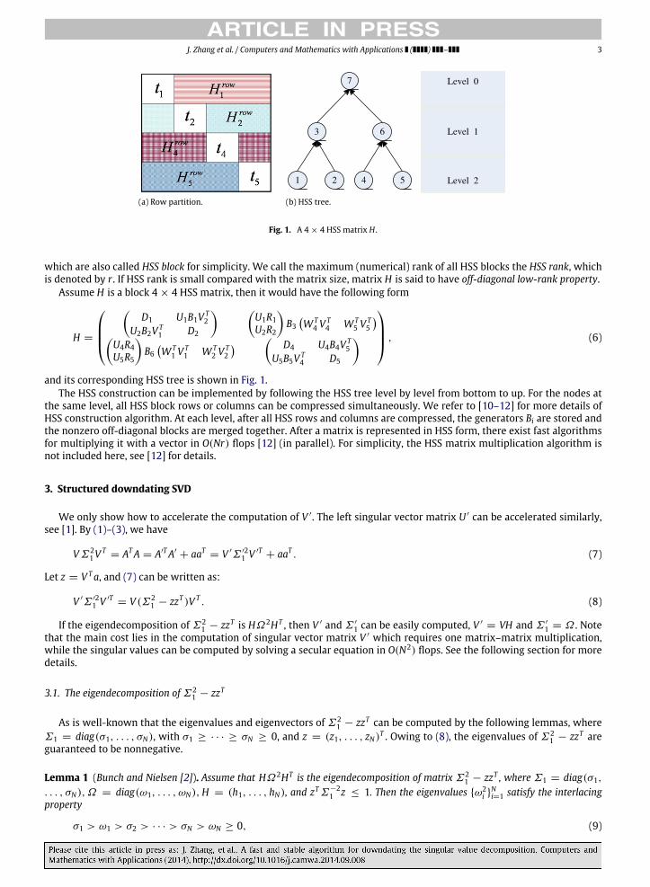
Fig. 1. A 4 × 4 HSS matrix H .

which are also called HSS block for simplicity. We call the maximum (numerical) rank of all HSS blocks the HSS rank, whichis denoted by r . If HSS rank is small compared with the matrix size, matrix H is said to have off-diagonal low-rank property.

Assume H is a block 4 × 4 HSS matrix, then it would have the following form

H =

D1 U1B1V T2

U2B2V T1 D2

U1R1U2R2

B3W T

4 VT4 W T

5 VT5

U4R4U5R5

B6W T

1 VT1 W T

2 VT2

D4 U4B4V T

5U5B5V T

4 D5

, (6)

and its corresponding HSS tree is shown in Fig. 1.The HSS construction can be implemented by following the HSS tree level by level from bottom to up. For the nodes at

the same level, all HSS block rows or columns can be compressed simultaneously. We refer to [10–12] for more details ofHSS construction algorithm. At each level, after all HSS rows and columns are compressed, the generators Bi are stored andthe nonzero off-diagonal blocks are merged together. After a matrix is represented in HSS form, there exist fast algorithmsfor multiplying it with a vector in O(Nr) flops [12] (in parallel). For simplicity, the HSS matrix multiplication algorithm isnot included here, see [12] for details.

3. Structured downdating SVD

We only show how to accelerate the computation of V ′. The left singular vector matrix U ′ can be accelerated similarly,see [1]. By (1)–(3), we have

VΣ21V

T= ATA = A′TA′

+ aaT = V ′Σ ′21 V ′T

+ aaT . (7)

Let z = V Ta, and (7) can be written as:

V ′Σ ′21 V ′T

= V (Σ21 − zzT )V T . (8)

If the eigendecomposition of Σ21 − zzT is HΩ2HT , then V ′ and Σ ′

1 can be easily computed, V ′= VH and Σ ′

1 = Ω . Notethat the main cost lies in the computation of singular vector matrix V ′ which requires one matrix–matrix multiplication,while the singular values can be computed by solving a secular equation in O(N2) flops. See the following section for moredetails.

3.1. The eigendecomposition of Σ21 − zzT

As is well-known that the eigenvalues and eigenvectors of Σ21 − zzT can be computed by the following lemmas, where

Σ1 = diag(σ1, . . . , σN), with σ1 ≥ · · · ≥ σN ≥ 0, and z = (z1, . . . , zN)T . Owing to (8), the eigenvalues of Σ21 − zzT are

guaranteed to be nonnegative.

Lemma 1 (Bunch and Nielsen [2]). Assume that HΩ2HT is the eigendecomposition of matrix Σ21 − zzT , where Σ1 = diag(σ1,

. . . , σN), Ω = diag(ω1, . . . , ωN),H = (h1, . . . , hN), and zTΣ−21 z ≤ 1. Then the eigenvalues ω2

i Ni=1 satisfy the interlacing

property

σ1 > ω1 > σ2 > · · · > σN > ωN ≥ 0, (9)

4 J. Zhang et al. / Computers and Mathematics with Applications ( ) –

Table 1The ranks of different off-diagonal blocks of H .

k 1 2 3 4 5 6 7 8 9 10 11 12

dim(×100) 1 2 3 4 5 6 7 8 9 10 11 12rank 16 18 21 22 23 22 24 23 23 24 23 25

and the following equation

f (ω) ≡ −1 +

Nj=1

z2jσ 2j − ω2

= 0. (10)

The eigenvectors are given by

hi =

z1

σ 21 − ω2

i, . . . ,

zNσ 2N − ω2

i

T Nj=1

z2j(σ 2

j − ω2i )

2. (11)

Note that the singular vectors cannot be computed directly from Eq. (11) since they may loss orthogonality [1]. One wayto solve this problem is to recompute the vector z, denoted by z, by using the following lemma.

Lemma 2 (See [16,1]). Given a diagonal matrix Σ1 = diag(σ1, . . . , σN) and a set of numbers ω2i

Ni=1 satisfying the interlacing

property

σ1 > ω1 > σ2 > · · · > σN > ωN ≥ 0, (12)

there exists a vector z = (z1, . . . , zN)T such that the eigenvalues of Σ21 − zzT are ω2

i Ni=1. The components of z are given by

|zi| =

(σ 2i − ω2

N)

i−1j=1

ω2j − σ 2

i

σ 2j − σ 2

i

N−1j=i

ω2j − σ 2

i

σ 2j+1 − σ 2

i, 1 ≤ i ≤ N, (13)

where the sign of zi can be chosen arbitrarily.

3.2. Low-rank property

Recall from Lemma 1, we find that H is a Cauchy-like matrix,

H =

α1z1σ 21 − ω2

1· · ·

αNz1σ 21 − ω2

N

α1z2σ 22 − ω2

1

...αNz2

σ 22 − ω2

N

......

...

α1zNσ 2N − ω2

1· · ·

αNzNσ 2N − ω2

N

, (14)

where αi = 1/N

j=1z2j

(σ 2j −ω2

i )2. Furthermore, it has off-diagonal low-rank structures, which is illustrated in the following

example.

Example 1. Assume H is a 2500× 2500 Cauchy-like matrix like (uivj

di−wj)ij, where u, v, d and w are 2500× 1 random vectors,

and the entries of d, w are interlacing: d1 > w1 > d2 > · · · > d2500 > w2500. The numerical ranks of the off-diagonalblocks Hk = H(m × k + 1 : end, 1 : m × k) with m = 100, are shown in Table 1, and the column dimensions are displayedin the second row of Table 1 (the column dimension is smaller than the row dimension). Here we use Matlab routine andε = 1.0e−13 to compute the numerical ranks. The results in Table 1 show that the off-diagonal ranks can be smaller thanthe sizes of the corresponding submatrices.

Remark 1. If the vectors d and w are interlacing, matrix H in Example 1 usually has off-diagonal low-rank property. Butit is not theoretically true. In [7], we show that the off-diagonal ranks depend on the distribution of the vectors d and w(probably u and v too). For example, when d and w are clustered, the off-diagonal rank may nearly equal the size of thecorresponding submatrix.

J. Zhang et al. / Computers and Mathematics with Applications ( ) – 5

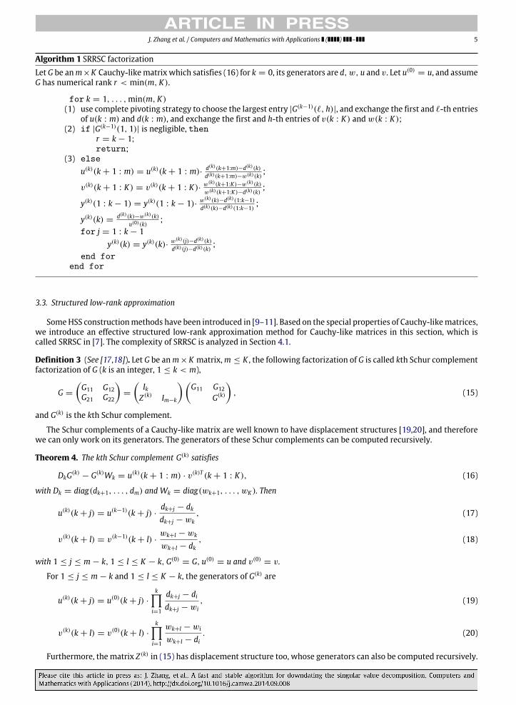
Algorithm 1 SRRSC factorizationLet G be anm×K Cauchy-likematrix which satisfies (16) for k = 0, its generators are d, w, u and v. Let u(0)

= u, and assumeG has numerical rank r < min(m, K).

for k = 1, . . . ,min(m, K)(1) use complete pivoting strategy to choose the largest entry |G(k−1)(ℓ, h)|, and exchange the first and ℓ-th entries

of u(k : m) and d(k : m), and exchange the first and h-th entries of v(k : K) and w(k : K);(2) if |G(k−1)(1, 1)| is negligible, then

r = k − 1;return;

(3) else

u(k)(k + 1 : m) = u(k)(k + 1 : m)· d(k)(k+1:m)−d(k)(k)d(k)(k+1:m)−w(k)(k)

;

v(k)(k + 1 : K) = v(k)(k + 1 : K)· w(k)(k+1:K)−w(k)(k)w(k)(k+1:K)−d(k)(k)

;

y(k)(1 : k − 1) = y(k)(1 : k − 1)· w(k)(k)−d(k)(1:k−1)d(k)(k)−d(k)(1:k−1)

;

y(k)(k) =d(k)(k)−w(k)(k)

u(0)(k);

for j = 1 : k − 1y(k)(k) = y(k)(k)· w(k)(j)−d(k)(k)

d(k)(j)−d(k)(k);

end forend for

3.3. Structured low-rank approximation

SomeHSS constructionmethods have been introduced in [9–11]. Based on the special properties of Cauchy-likematrices,we introduce an effective structured low-rank approximation method for Cauchy-like matrices in this section, which iscalled SRRSC in [7]. The complexity of SRRSC is analyzed in Section 4.1.

Definition 3 (See [17,18]). Let G be anm×K matrix,m ≤ K , the following factorization of G is called kth Schur complementfactorization of G (k is an integer, 1 ≤ k < m),

G =

G11 G12G21 G22

=

IkZ (k) Im−k

G11 G12

G(k)

, (15)

and G(k) is the kth Schur complement.

The Schur complements of a Cauchy-like matrix are well known to have displacement structures [19,20], and thereforewe can only work on its generators. The generators of these Schur complements can be computed recursively.

Theorem 4. The kth Schur complement G(k) satisfies

DkG(k)− G(k)Wk = u(k)(k + 1 : m) · v(k)T (k + 1 : K), (16)

with Dk = diag(dk+1, . . . , dm) and Wk = diag(wk+1, . . . , wK ). Then

u(k)(k + j) = u(k−1)(k + j) ·dk+j − dkdk+j − wk

, (17)

v(k)(k + l) = v(k−1)(k + l) ·wk+l − wk

wk+l − dk, (18)

with 1 ≤ j ≤ m − k, 1 ≤ l ≤ K − k,G(0)= G, u(0)

= u and v(0)= v.

For 1 ≤ j ≤ m − k and 1 ≤ l ≤ K − k, the generators of G(k) are

u(k)(k + j) = u(0)(k + j) ·

ki=1

dk+j − didk+j − wi

, (19)

v(k)(k + l) = v(0)(k + l) ·

ki=1

wk+l − wi

wk+l − di. (20)

Furthermore, the matrix Z (k) in (15) has displacement structure too, whose generators can also be computed recursively.

6 J. Zhang et al. / Computers and Mathematics with Applications ( ) –

Theorem 5. The generators of Z (k) satisfy the following displacement equation

D(k)2 Z (k)

− Z (k)D(k)1 = u(k)(k + 1 : m) · y(k)(1 : k), (21)

where D(k)1 = diag(d1, . . . , dk),D

(k)2 = diag(dk+1, . . . , dm), u(k)(k + 1 : m) are computed recursively by (17), and

y(k)(i) =

y(k−1)(i) ·

wk − didk − di

if 1 ≤ i ≤ k − 1,k−1j=1

dk − wj

dk − dj·dk − wk

u(0)(i)if i = k.

(22)

Note that if matrix (15) which corresponds to an HSS block is rank-deficient, at some step the entries of G(k) wouldbecome negligible. Thus by ignoring G(k), we can get a low-rank approximation to G,

G ≈

I

Z (k)

G11 G12

. (23)

To have better numerical stability, we incorporate pivoting into the factorization (15) since pivoting does not destroy theCauchy-like structure. The complete pivoting is best for stability but it may deteriorate the speed. For some more efficientpivoting strategies, we refer to [7,20,18]. The whole structure of SRRSC is illustrated in Algorithm 1.

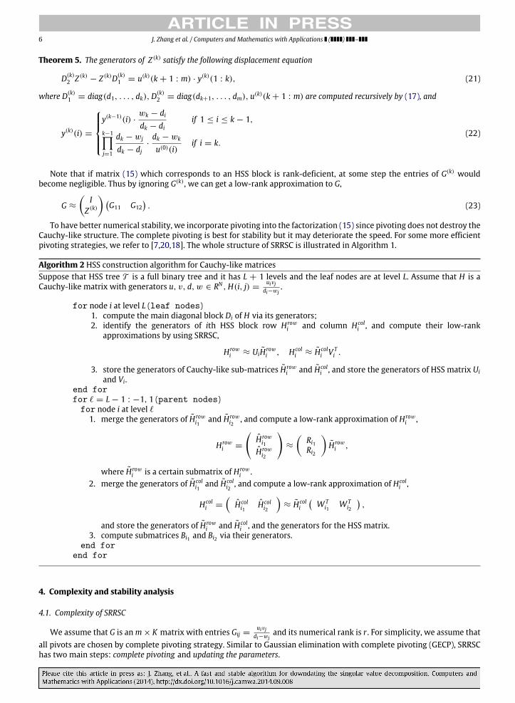
Algorithm 2 HSS construction algorithm for Cauchy-like matricesSuppose that HSS tree T is a full binary tree and it has L + 1 levels and the leaf nodes are at level L. Assume that H is aCauchy-like matrix with generators u, v, d, w ∈ RN ,H(i, j) =

uivjdi−wj

.

for node i at level L (leaf nodes)1. compute the main diagonal block Di of H via its generators;2. identify the generators of ith HSS block row Hrow

i and column Hcoli , and compute their low-rank

approximations by using SRRSC,

Hrowi ≈ UiHrow

i , Hcoli ≈ Hcol

i V Ti .

3. store the generators of Cauchy-like sub-matrices Hrowi and Hcol

i , and store the generators of HSS matrix Uiand Vi.

end forfor ℓ = L − 1 : −1, 1 (parent nodes)for node i at level ℓ

1. merge the generators of Hrowi1

and Hrowi2

, and compute a low-rank approximation of Hrowi ,

Hrowi =

Hrow

i1Hrow

i2

≈

Ri1Ri2

Hrow

i ,

where Hrowi is a certain submatrix of Hrow

i .2. merge the generators of Hcol

i1and Hcol

i2, and compute a low-rank approximation of Hcol

i ,

Hcoli =

Hcol

i1Hcol

i2

≈ Hcol

i

W T

i1W T

i2

,

and store the generators of Hrowi and Hcol

i , and the generators for the HSS matrix.3. compute submatrices Bi1 and Bi2 via their generators.

end forend for

4. Complexity and stability analysis

4.1. Complexity of SRRSC

We assume that G is anm× K matrix with entries Gij =uivj

di−wjand its numerical rank is r . For simplicity, we assume that

all pivots are chosen by complete pivoting strategy. Similar to Gaussian elimination with complete pivoting (GECP), SRRSChas two main steps: complete pivoting and updating the parameters.

J. Zhang et al. / Computers and Mathematics with Applications ( ) – 7

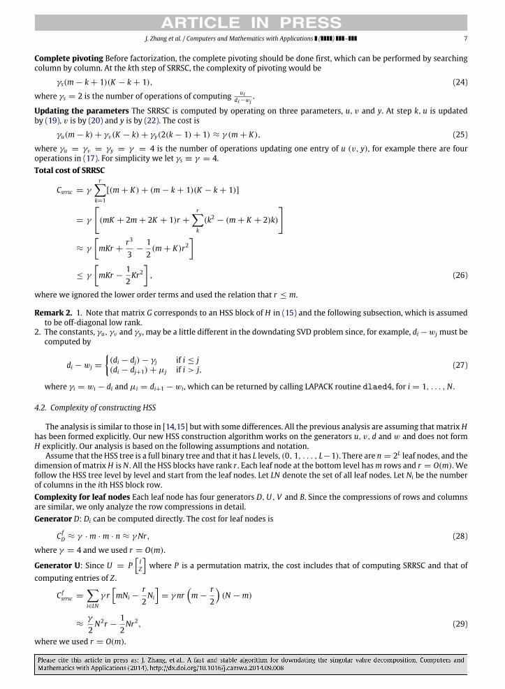
Complete pivoting Before factorization, the complete pivoting should be done first, which can be performed by searchingcolumn by column. At the kth step of SRRSC, the complexity of pivoting would be

γs(m − k + 1)(K − k + 1), (24)

where γs = 2 is the number of operations of computing uℓ

dℓ−wj.

Updating the parameters The SRRSC is computed by operating on three parameters, u, v and y. At step k, u is updatedby (19), v is by (20) and y is by (22). The cost is

γu(m − k) + γv(K − k) + γy(2(k − 1) + 1) ≈ γ (m + K), (25)

where γu = γv = γy = γ = 4 is the number of operations updating one entry of u (v, y), for example there are fouroperations in (17). For simplicity we let γs ≡ γ = 4.Total cost of SRRSC

Csrrsc = γ

rk=1

[(m + K) + (m − k + 1)(K − k + 1)]

= γ

(mK + 2m + 2K + 1)r +

rk

(k2 − (m + K + 2)k)

≈ γ

mKr +

r3

3−

12(m + K)r2

≤ γ

mKr −

12Kr2

, (26)

where we ignored the lower order terms and used the relation that r ≤ m.

Remark 2. 1. Note that matrix G corresponds to an HSS block of H in (15) and the following subsection, which is assumedto be off-diagonal low rank.

2. The constants, γu, γv and γy, may be a little different in the downdating SVD problem since, for example, di − wj must becomputed by

di − wj =

(di − dj) − γj if i ≤ j(di − dj+1) + µj if i > j, (27)

where γi = wi − di and µi = di+1 − wi, which can be returned by calling LAPACK routine dlaed4, for i = 1, . . . ,N .

4.2. Complexity of constructing HSS

The analysis is similar to those in [14,15] but with some differences. All the previous analysis are assuming that matrix Hhas been formed explicitly. Our new HSS construction algorithm works on the generators u, v, d and w and does not formH explicitly. Our analysis is based on the following assumptions and notation.

Assume that the HSS tree is a full binary tree and that it has L levels, (0, 1, . . . , L−1). There are n = 2L leaf nodes, and thedimension of matrix H is N . All the HSS blocks have rank r . Each leaf node at the bottom level hasm rows and r = O(m). Wefollow the HSS tree level by level and start from the leaf nodes. Let LN denote the set of all leaf nodes. Let Ni be the numberof columns in the ith HSS block row.Complexity for leaf nodes Each leaf node has four generators D,U, V and B. Since the compressions of rows and columnsare similar, we only analyze the row compressions in detail.Generator D: Di can be computed directly. The cost for leaf nodes is

C fD ≈ γ · m · m · n ≈ γNr, (28)

where γ = 4 and we used r = O(m).

Generator U: Since U = PIZ

where P is a permutation matrix, the cost includes that of computing SRRSC and that of

computing entries of Z .

C fsrrsc =

i∈LN

γ rmNi −

r2Ni

= γ nr

m −

r2

(N − m)

≈γ

2N2r −

12Nr2, (29)

where we used r = O(m).

8 J. Zhang et al. / Computers and Mathematics with Applications ( ) –

Since the (i, j)th entry of Z is Zij =uiyjdi−dj

, after obtaining the generators of Z the cost of computing Z isi∈LN

γ (m − r)r ≈ γNr.

Thus, the cost of computing U for all leaf nodes is

C fU =

γ

2N2r + O(Nr − Nr2).

Generator V: It needs the same operations as U, C fV = C f

U .Generator B: Each Bi at the bottom level is a r × r matrix. The cost is

C fB =

i∈LN

γ · r · r ≈ γNr,

where we used r = O(m) and there are n leaf nodes.Therefore, the total cost for leaf nodes is

C f= C f

D + C fU + C f

V + C fB = γN2r + O(Nr − Nr2).

Complexity for parent nodes For a parent node i, letUi =

Ri1Ri2

,Vi =

Wi1Wi2

and Bi. Then, similar to the analysis of leaf nodes,

we can compute the cost of parent nodes level by level. Note that there are 2ℓ nodes at level ℓ, and the row dimension ofeach HSS block row is 2r . No operation is needed for the root node. The total cost for all parent nodes is

Cp= CpU + CpV + Cp

B =32γN2r + O(Nr2).

Therefore, the total complexity of constructing HSS matrix is about

C = C f+ Cp

=52γN2r + O(Nr2) = 10N2r + O(Nr2).

Remark 3. The HSS construction algorithms based on SRRSC need O(N2r) operations. The main advantage of using SRRSCis that it only needs O(N) memory which can potentially work on very large matrices. It is easy to see that the complexityof our downdating algorithm, shown in Algorithm 3, is also O(N2r) flops.

4.3. Numerical stability of SRRSC

An error analysis for the LU factorization of Cauchy-like matrices appeared in [21]. Since the Cauchy-like matricesconsidered in this paper have displacement rank one, using the same techniques as in [21], it is easy to show that thebackward stability of SRRSC is related to that of the classical Gaussian elimination, see also [22]. Therefore, the algorithm isbackward stable, which is also illustrated as follows.

Theorem 6. Assume that no overflows and underflows were encountered during the computation and ε is a unit roundoff. Thenthe computed factors Z (k), G(k) satisfies Z (k)

= Z (k)+ ∆Z (k) and G(k)

= G(k)+ ∆G(k), where

|∆Z (k)| ≤ γ8k+1|Z (k)

|, |∆G(k)| ≤ γ8k+3|G(k)

|

γk =

kε1 − kε

. (30)

Proof. Assume that permutation has been done beforehand. By Theorems 4 and 5,

u(k)(k + l) = u(0)(k + l) ·

kj=1

dk+l − djdk+l − wj

, (31)

y(k)(i) =

i−1j=1

di − wj

di − dj·

kj=i+1

di − wj

di − dj·di − wi

u(0)(i). (32)

A straightforward error analysis implies

Z (k)(i, j) = flu(k)(k + i)y(k)(j)

dk+i − dj

= Z (k)(i, j)δ(k)

i,j , (33)

J. Zhang et al. / Computers and Mathematics with Applications ( ) – 9

where

(1 − ε)6k+1

(1 + ε)2k≤ δ

(k)i,j ≤

(1 + ε)6k+1

(1 − ε)2k. (34)

The similar arguments can be applied to G(k) and get its rounding error bound.

Corollary 7. The computed factorization G =

Ik

Z(k) Im−k

G11 G12

G(k)

satisfies G = G + ∆E(k), if we define L =

Ik

Z(k) Im−k

and F =

G11 G12

G(k)

, then

|∆E(k)| ≤ [(16k + 4)ε + O(ε2)]|L||F |. (35)

Proof. From the standard error analysis, the computed G = LF satisfies

LF = (L + ∆L)(F + ∆F) = LF + ∆E(k) (36)

where

|∆L| ≤ γ8k+1|L|, |∆F | ≤ γ8k+3|F |. (37)

The bound (35) can be derived from (30) and (37).

Algorithm 3 Downdating the SVDGiven an M × N (M > N) matrix A and its SVD, A = UΣV T , assume the bottom vector aT is to be deleted.

1. Extract the submatrix Σ1 from Σ and compute z = V Ta;2. Compute the eigendecomposition of Σ2

1 − zzT by solving secular equations and store the generators of matrix H;3. Use SRRSC to construct an HSS approximation to H

H ≈ H,

where H is an HSS matrix;4. Compute the right singular vectors of A′ by using fast HSS matrix–matrix multiplications

V ′= VH.

5. Numerical results

We use our algorithm to solve the following specific problem,

Given V , Σ1 and a, compute V ′ and Σ ′

1.

The algorithm that we used is summarized in Algorithm 3.The following examples are tested on a laptop with 4 GB memory and Intel(R) Core(TM) i7-2640M CPU. For compilation

we used Intel fortran compiler (ifort) and the optimization flag -O2, and then linked the codes to the optimized BLAS andLAPACK library, Intel MKL (composer_xe_2013_sp1).

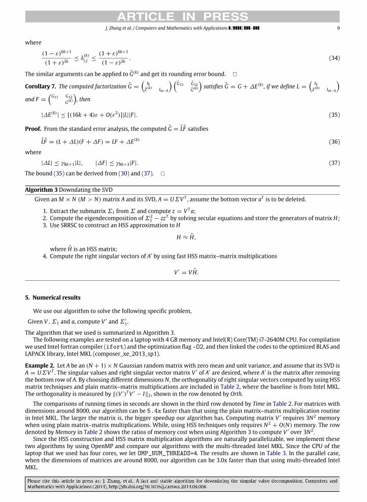
Example 2. Let A be an (N + 1) × N Gaussian randommatrix with zero mean and unit variance, and assume that its SVD isA = UΣV T . The singular values and right singular vector matrix V ′ of A′ are desired, where A′ is the matrix after removingthe bottom row of A. By choosing different dimensions N , the orthogonality of right singular vectors computed by using HSSmatrix techniques and plain matrix–matrix multiplications are included in Table 2, where the baseline is from Intel MKL.The orthogonality is measured by ∥(V ′)TV ′

− I∥2, shown in the row denoted by Orth.

The comparisons of running times in seconds are shown in the third row denoted by Time in Table 2. For matrices withdimensions around 8000, our algorithm can be 5.4x faster than that using the plain matrix–matrix multiplication routinein Intel MKL. The larger the matrix is, the bigger speedup our algorithm has. Computing matrix V ′ requires 3N2 memorywhen using plain matrix–matrix multiplications. While, using HSS techniques only requires N2

+ O(N) memory. The rowdenoted byMemory in Table 2 shows the ratios of memory cost when using Algorithm 3 to compute V ′ over 3N2.

Since the HSS construction and HSS matrix multiplication algorithms are naturally parallelizable, we implement thesetwo algorithms by using OpenMP and compare our algorithms with the multi-threaded Intel MKL. Since the CPU of thelaptop that we used has four cores, we let OMP_NUM_THREADS=4. The results are shown in Table 3. In the parallel case,when the dimensions of matrices are around 8000, our algorithm can be 3.0x faster than that using multi-threaded IntelMKL.

10 J. Zhang et al. / Computers and Mathematics with Applications ( ) –

Table 2The comparison of orthogonality and speedups with MKL, k denotes onethousand.

Dim 1k × 1k 3k × 3k 4k × 4k 5k × 5k 8k × 8k

Orth. HSS 1.7e−14 3.5e−14 4.9e−14 5.4e−14 7.4e−14MKL 1.7e−14 3.7e−14 5.1e−14 5.9e−14 8.0e−14

Time HSS 7.8e−02 0.7e+00 1.2e+00 1.9e+00 5.0e+00MKL 9.4e−02 1.7e+00 3.7e+00 6.9e+01 2.7e+01

Speedup 1.2x 2.5x 3.0x 3.6x 5.4xMemory 0.65 0.53 0.46 0.45 0.41

Table 3The results for parallel implementation, k denotes one thousand.

Dim 1k × 1k 3k × 3k 4k × 4k 5k × 5k 8k × 8k

Orth. HSS 1.6e−14 3.5e−14 4.9e−14 5.5e−14 8.0e−14MKL 1.7e−14 3.7e−14 5.1e−14 5.9e−14 7.5e−14

Time HSS 5.9e−02 7.5e−01 8.9e−01 1.4e+00 3.6e+00MKL 6.3e−02 1.3e+00 1.7e+00 3.1e+00 1.1e+01

Speedup 1.1x 1.7x 1.9x 2.2x 3.0x

6. Conclusion

In this paper, we propose an accelerated downdating SVD algorithm by using HSS matrix techniques, which was firstintroduced in [1]. The improved downdating algorithm is summarized in Algorithm 3, which can reduce the complexity offloating-point operations and storage cost significantly, especially for matrices with large dimensions. We use SRRSC [8,7]to construct HSS approximations. In Section 4, the complexities of SRRSC and HSS construction algorithm based on SRRSCare analyzed in detail. Furthermore, the rounding error analysis of SRRSC is also included, which is shown to be backwardstable. Comparisons with sequential and multi-threaded Intel MKL show that using HSS techniques to compute V ′ can be3x–5x faster than using plain matrix–matrix multiplications implemented in Intel MKL for large matrices.

Acknowledgments

This work is partially supported by National Natural Science Foundation of China (No. 11401580), NSF of Hunan Provincein China (No. 13JJ2001 and 13JJ4011) and Doctoral Foundation of Ministry of Education of China (No. 20114307120021).

References

[1] M. Gu, S.C. Eisenstat, Downdating the singular value decomposition, SIAM J. Matrix Anal. Appl. 16 (1995) 793–810.[2] J.R. Bunch, C.P. Nielsen, Updating the singular value decomposition, Numer. Math. 31 (1978) 111–129.[3] M. Moonen, P. Van Dooren, J. Vandewalle, A singular value decomposition updating algorithm for subspace tracking, SIAM J. Matrix Anal. Appl. 13

(1992) 1015–1038.[4] J. Barlow, P.A. Yoon, H. Zha, An algorithm and a stability theory for downdating the ULV decomposition, BIT 36 (1996) 14–40.[5] G. Stewart, Determining rank in the presense of error, in: Linear Algebra for Large Scale and Real-time Applications, vol. 232, 1993, pp. 275–291.[6] D. Witter, M. Berry, Downdating the latent semantic indexing model for conceptual information retrieval, Comput. J. 41 (1998) 589–601.[7] S. Li, M. Gu, L. Cheng, X. Chi, M. Sun, An accelerated divide-and-conquer algorithm for the bidiagonal singular value problem, SIAM J. Matrix Anal.

Appl. 35 (2014) 1038–1057.[8] M. Gu, A numerically stable superfast Toeplitz solver, in: Presentations in Berkeley Matrix Computations and Scientific Computing Seminar and SIAM

LA09, 2009, http://math.berkeley.edu/~mgu/Seminar/Fall2009/ToeplitzSeminarTalk.pdf.[9] J. Xia, S. Chandrasekaran, M. Gu, X. Li, Fast algorithms for hierarchically semiseparable matrices, Numer. Linear Algebra Appl. 17 (2010) 953–976.

[10] S. Chandrasekaran, M. Gu, T. Pals, Fast and Stable Algorithms for Hierarchically Semiseparable Representations, Tech. Report, University of California,Berkeley, CA, 2004.

[11] S. Chandrasekaran, M. Gu, T. Pals, A fast ULV decomposition solver for hierarchical semiseparable representations, SIAM J. Matrix Anal. Appl. 28 (2006)603–622.

[12] W. Lyons, Fast algorithms with applications to PDEs (Ph.D. thesis), University of California, Santa Barbara, 2005.[13] M. Gu, S.C. Eisenstat, A Stable and Fast Algorithm for Updating the Singular Value Decomposition, Tech. Report, RR-966, Yale University, 1994.[14] J. Xia, M. Gu, Robust approximate Cholesky factorization of rank-structured symmetric positive definite matrices, SIAM J. Matrix Anal. Appl. 31 (2010)

2899–2920.[15] S. Li, M. Gu, C.J. Wu, J. Xia, New efficient and robust HSS Cholesky factorization of symmetric positive definite matrices, SIAM J. Matrix Anal. Appl. 33

(2012) 886–904.[16] K. Löwner, Über monotone Matrixfunktionen, Math. Z. 38 (1934) 176–216.[17] R.W. Cottle, Manifestations of the Schur complement, Linear Algebra Appl. 8 (1974) 189–211.[18] C. Pan, On the existence and computation of rank revealing LU factorizations, Linear Algebra Appl. 316 (2000) 199–222.[19] I. Gohberg, T. Kailath, V. Olshevsky, Fast Gaussian elimination with partial pivoting for matrices with displacement structure, Math. Comp. 64 (1995)

1557–1576.[20] M. Gu, Stable and efficient algorithms for structured systems of linear equations, SIAM J. Matrix Anal. Appl. 19 (1998) 279–306.[21] D. Sweet, R. Brent, Error analysis of a fast partial pivoting method for structured matrices, in: Proceedings of the SPIE-1995, vol. 2563, pp. 266–280.[22] T. Boros, T. Kailath, V. Olshevsky, Pivoting and backward stability of fast algorithms for solving Cauchy linear equations, Linear Algebra Appl. 343

(2002) 63–99.