1

A Fast and Stable Penalty Method for Rigid BodySimulationEvan Drumwright

University of Southern Californiadrumwrig@robotics.usc.edu

Abstract— Two methods have been used extensively to modelresting contact for rigid body simulation. The first approach, thepenalty method, applies virtual springs to surfaces in contact tominimize interpenetration. This method, as typically implemented,results in oscillatory behavior and considerable penetration. Thesecond approach, based on formulating resting contact as a linearcomplementarity problem, determines the resting contact forcesanalytically to prevent interpenetration. The analytical methodexhibits expected-case polynomial complexity in the number ofcontact points, and may fail to find a solution in polynomial timewhen friction is modeled. We present a fast penalty method thatminimizes oscillatory behavior and leads to little penetration duringresting contact; our method compares favorably to the analyticalmethod with regard to these two measures, while exhibiting muchfaster performance both asymptotically and empirically.

I. INTRODUCTION

The problem of contact modeling is one of the greatestobstacles to simulating rigid bodies. Tradeoffs must bemade between speed, numerical stability, and accuracy.Recent work has approached contact modeling in differentways: solving for contact forces analytically [1], treatingcollision and resting contact using impulses [2], [3], andformulating the time-stepping equations to respect non-penetration constraints [4]. Nevertheless, these solutionsmay be too slow for or otherwise inappropriate for somesimulation domains. For example, both robotic and hapticsimulation require high frequency integration, and the sim-plest method, the penalty method [5] often remains the bestsolution in such cases.

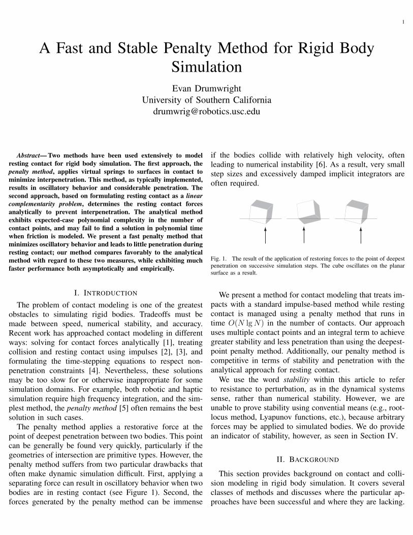
The penalty method applies a restorative force at thepoint of deepest penetration between two bodies. This pointcan be generally be found very quickly, particularly if thegeometries of intersection are primitive types. However, thepenalty method suffers from two particular drawbacks thatoften make dynamic simulation difficult. First, applying aseparating force can result in oscillatory behavior when twobodies are in resting contact (see Figure 1). Second, theforces generated by the penalty method can be immense

if the bodies collide with relatively high velocity, oftenleading to numerical instability [6]. As a result, very smallstep sizes and excessively damped implicit integrators areoften required.

Fig. 1. The result of the application of restoring forces to the point of deepestpenetration on successive simulation steps. The cube oscillates on the planarsurface as a result.

We present a method for contact modeling that treats im-pacts with a standard impulse-based method while restingcontact is managed using a penalty method that runs intime O(N lg N) in the number of contacts. Our approachuses multiple contact points and an integral term to achievegreater stability and less penetration than using the deepest-point penalty method. Additionally, our penalty method iscompetitive in terms of stability and penetration with theanalytical approach for resting contact.

We use the word stability within this article to referto resistance to perturbation, as in the dynamical systemssense, rather than numerical stability. However, we areunable to prove stability using convential means (e.g., root-locus method, Lyapunov functions, etc.), because arbitraryforces may be applied to simulated bodies. We do providean indicator of stability, however, as seen in Section IV.

II. BACKGROUND

This section provides background on contact and colli-sion modeling in rigid body simulation. It covers severalclasses of methods and discusses where the particular ap-proaches have been successful and where they are lacking.

2

A. Separation of methods for contact and collisionMoore and Wilhelms [5] provided some of the earliest

work toward combining rigid-body simulation and com-puter graphics. They introduced a popular paradigm inrigid-body simulation: contacts and collisions are separatedusing a threshold velocity, and handled using differentmeans. For example, Moore and Wilhelms determine theimpulse-velocities1 for collision handling by algebraicallysolving a system of 15 equations with 15 variables usingconservation of momentum and Newton’s law of restitu-tion.2 For low relative velocity projected along the contactnormal, Moore and Wilhelms applied a single virtual springto mitigate interpenetration.

Moore and Wilhelms’ virtual spring method is discontin-uous. They apply a restorative force to the point of deepestpenetration (or nearest approach), and do not apply forceonce the objects begin separating (even if still penetrat-ing). This discontinuous method can be readily extendedto perform analogously to a proportional-derivative (PD)controller (using zero desired penetration depth and zerodesired relative normal velocity) or even a proportional-integrative-derivative (PID) controller, as is done in SectionIII-B.

B. Analytical solutions to constrained contactResting contact can be modeled by determining the

appropriate constraining forces analytically. For bilateral(i.e., joint) constraints, a Lagrange-multiplier approach canbe used to solve for the constraining forces in O(n) time [8](n is the number of links in the loop-free, articulated body).Unfortunately, unilateral constraints cannot be resolved inthis manner. The principal way of determining contactforces is by formulating the system as a linear comple-mentarity problem (LCP) [9]. A linear complementarityproblem takes the form:

Ax + b = w

x ≥ 0

w ≥ 0

xTw = 0

where A is a n × n matrix, and x, w, and b are n × 1vectors. Given A and b, the goal is to solve for vectors

1The term impulse-velocity is used because true (i.e., infinite force over aninfinitesimally small time interval) impulses cannot be used in discrete timerigid body simulation. However, the velocities of colliding objects are updatedas if an impulse had been applied.

2Hahn [7] also solved for collision impulses analytically, but did not handleresting contact separately, thereby leading to drift.

w and x that satisfy the constraints. In the case of contactconstraints, x and w are the vectors of normal forces andrelative accelerations, respectively; the nth element of eachdenotes the signed magnitude of the vector when projectedalong the nth contact normal at the nth contact point. A andb can be computed in time O(n2), where n is the numberof contact points, if the bodies in contact are unarticulated[10]. If the bodies in contact are articulated and possessm links, A and b can be computed in time O(mn) [11]or time (m3n) [12]. Given b and the symmetric, positive-definite matrix A, the desired normal force magnitudes canbe computed in worst-case exponential time but expectedpolynomial time in the number of contact points [13].

When friction is added to the system, the problembecomes much harder computationally. For dynamic (slid-ing) friction, the number of constraints per contact pointincreases to two. Far more troubling, however, is thatthe matrix A generally becomes non-symmetric and non-positive definite. As Cottle notes [13], solving a LCPunder such conditions is effectively as difficult as quadraticprogramming (i.e., NP-hard in general). Managing static(sticking) friction in this model is no easier. Static frictionconstrains the magnitude of the applied friction force atany contact point to be no greater than the coefficientof friction times the magnitude of the normal force. Themagnitudes of the two tangent directions at the contact pointare thus constrained nonlinearly (i.e.,

√f 2

t1 + f 2t2 ≤ µfN ),

and the problem becomes a nonlinear complementarityproblem (NCP); as might be expected, solving a NCPis also as difficult as solving a quadratic programmingproblem. Indeed, Lostedt [14] used quadratic programmingto compute the normal and frictional forces analytically.Baraff [1] presented a pivoting algorithm for computing thenormal and frictional forces in O(n4) time; this algorithm isnot guaranteed to terminate for systems with friction. As anaside, the problem of determining contact forces necessaryto ensure that normal and frictional constraints are satisfiedis NP-hard [15]. It is also possible that such a problem isinconsistent, meaning that no non-impulsive forces can bedetermined to satisfy all of the constraints [1].

Finally, approaches that compute static friction forcesanalytically, such as the method described above, exhibita significant limitation with regard to control of articulatedbodies. The equations used to compute inverse dynamicsand the equations for determining sticking frictional forcesare coupled, so standard inverse dynamics algorithms (i.e.,

3

Recursive Newton-Euler [16]) cannot be employed.3

C. Impulse-based simulationMirtich’s seminal thesis on impulse-based simulation [2])

modeled all contacts using trains of impulse-velocities.Mirtich not only provided an algorithm for applying im-pulses to articulated bodies simulated using generalized(rather than maximal) coordinates, but also for computingimpulses using the Stronge hypothesis [17], which ensuresthat energy is conserved during collisions with Coulombfriction.

Mirtich’s work suffers from a few weaknesses and limita-tions. For resting contact, he applies restitution coefficientsabove one to combat drift, which is somewhat unappealing.Additionally, this mechanism experiences significant slow-down when objects are resting upon another (i.e., stacked),as a result of the numerous propagated impulses. Mirtich’smethod for determining the proper impulse to apply to anarticulated body runs in time O(n) (n being the numberof links in the body), but the constant factor is somewhathigh.

D. Formulating the ODEs with constraintsA number of approaches toward rigid body simulation

have investigated explicit time-stepping formulations [18],[19], [20], [21], [22], [23], [24], [4], [25], [26], [27].The most recent of these approaches have combined theNewton-Euler equations for motion with joint and non-penetration constraints to produce methods that do not re-quire separation into contact and collision. Non-penetrationand frictional constraints are incorporated into the integra-tion formula, and positions and velocities that satisfy themodel for the next time step are determined using a LCPsolver. These methods can typically prove the existence ofsolutions that satisfy the constraints when the integrationstep size is sufficiently low (i.e., inconsistent configurationsdo not occur).

Explicit time-stepping formulations are subject to threeparticular limitations. First, the computational burden canbe significant: the mixed-LCP (unilateral and bilateralconstraint) pivoting algorithm used by the more popularmethods runs in time O(n4) in the number of constraints inthe expected case. Second, interpenetration generally occursdue to drift, and must be corrected via an ad hoc post-stabilization method. Finally, these approaches have yet to

3Such inverse dynamics algorithms can be used, but the outputs will beincorrect. It remains to be seen whether standard inverse dynamics algorithmscould still function in a useful feedforward capacity while not accounting forsticking frictional forces

be extended to articulated bodies formulated in generalizedcoordinates.

E. Effective treatment of contacts and impacts using im-pulses

Guendelman et al. [3] introduced a novel idea to rigidbody simulation: by interleaving collision and contact be-tween integration of the velocity and position equationsof motion, both contact and collision can be modeledwith impulses without resorting to Mirtich’s microimpulsemethod for resting contact. Guendelman et al.’s simulationparadigm consists of the following four phases:

1) modeling collisions (velocity update)2) integration of acceleration (v = F/m and ω = J−1τ )3) modeling contact (velocity update)4) integration of velocity (position update)Forces are incorporated in step (2). Forces that lead

to interpenetration are effectively cancelled in step (3).In addition to this particular innovation, [3] is also themost notable work on simulation of rigid bodies with non-convex geometries. Guendelman et al.’s work was laterextended to articulated bodies (using maximal coordinates)by Weinstein et al. [28], [29].

The work of Guendelman et al. is subject to somelimitations. First, the use of Newton’s law of restitutionfor handling frictional collision (or contact) is subject toenergy gain, as Stronge noted in his thesis [17]; the authorscould have used Mirtich’s method to address this problem,but it is computationally expensive. Second, the method ofGuendelman et al. suffers from drift for objects in restingcontact, resulting in increasing interpenetration over time.Third, Guendelman et al. do not regress the simulation tothe time of impact; skipping this step avoids significantcomputation, but often results in noticeable visual arti-facts unless the step size is small or velocities are low.Finally, Guendelman et al. requires considerable overheadper articulated body formulated in generalized coordinatesto determine the collision matrix, K, as is done in [2].

The broader issue with impulse-based methods, includingthe work of both Mirtich and Guendelman et al., is thatthey have traditionally been local methods: impulses areapplied sequentially at points of intersection. This paradigmgenerally works quite well for unarticulated bodies. Forarticulated bodies under contact constraints that inducekinematic loops (e.g., a biped standing with both feettouching the ground), the constraints will likely not besatisfied after sequential application of impulses. This situ-ation arises frequently under Coulomb friction, particularlysticking friction. Guendelmann et al. attempt to alleviate

4

this problem by performing several iterations of contactand collision processing. However, there is no guarantee ofconvergence to a stable solution, nor do there exist anyheuristics for choosing the number of iterations. Globalimpulse-based methods, as suggested by Baraff [30] andSchmidl and Milenkovic [31], can potentially avoid theseissues, though the computation required is essentially iden-tical to that described in Section II-B.

F. Analytical computation of penalty forcesHasegawa and Sato [32] developed a method for an-

alytical computation of penalty forces; their particularapplication domain is haptic simulation, which requireshigh-frequency updates to drive force displays [33], andfor which solving LCPs is too slow. To compute thepenalty forces, the authors determine the intersection ofthe two convex polyhedra in contact using the algorithmof Preparata and Shamos [34] (running time of O(N lg N),where N = m + n and m and n are the features in eachpolyhedron), and then integrate over the triangular volumeof intersection.

The method of Hasegawa and Sato is quite fast comparedto LCP methods, but suffers from two key limitations. First,determining the intersection of convex polyhedra suffersfrom degeneracies unless exact (and slow) arithmetic isutilized. If the volume of integration is quite small, thenthe intersection algorithm will likely fail, and penalty forceswill not be computed; greater penetration will be the result.Second, the constant factor for this algorithm is quite high.The Muller-Preparata algorithm requires an intricate oper-ation to determine a point interior to both polyhedra andtwo 3D convex hull operations. Additionally, the integrationformulae for computing the penalty forces requires severalthousand floating-point operations per triangle.

III. METHOD

Determining exact contact forces necessary to satisfynonpenetration constraints is NP-hard, as noted in the previ-ous section. Most of the methods discussed in the previoussection are approximation methods; exact solutions are notcomputed in order to maintain acceptable simulation fre-quency. These methods make tradeoffs between accuracy,speed, and numerical stability. The method introduced inthis section is not an exception. It was developed towardrobotic simulation, which requires generalized coordinateformulations, maximal speed, and minimal oscillations aris-ing from contact modeling.

Our method uses the normal velocity threshold paradigmintroduced by Moore and Wilhelms [5] to classify contacts

No contact

new impacting contact

Impact response

no longer contact

!i, si

n > 0

recurring contact

!i, sin " 0,#j, sj

n < $!

reimpact (bounce)

Impact method

Penalty method

recurring contact!i,"! # si

n # 0

no longer contact recurring contact

new resting contact

!i, si

n < "!

!j,"! # si

n

bodyimpacted

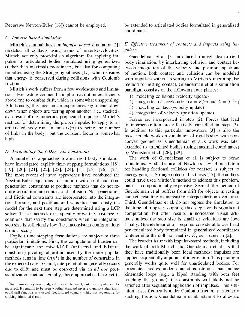
Fig. 2. The state transition diagram tracks the contact phase between twobodies. Note that after two bodies are in resting contact (i.e., the penalty methodstate), the impact method can only be triggered by a third body impactingone of the two. ε is a floating-point value very near to zero, and si

n is therelative normal velocity at the ith contact point (the bodies are separatingwhen si

n > 0).

as either impacting or resting. The sequential impulse-based method of Baraff [35], modified to handle frictionalcollisions as in [5], [7], [3] and applied at the centroid ofthe contact surface, treats impacts; a penalty method han-dles resting contacts. Unlike traditional velocity thresholdapproaches, we apply our resting contact method duringcontinuous contact regardless of the relative normal veloc-ity; once continuous contact has begun, impacting contactcan only be triggered if one of the bodies is impacted bya third body. This approach allows us to drive the velocitythreshold to very near zero, thereby addressing the criticismthat the threshold is set in an ad hoc manner. Figure 2depicts the transitions between contact phases for a pair ofbodies.

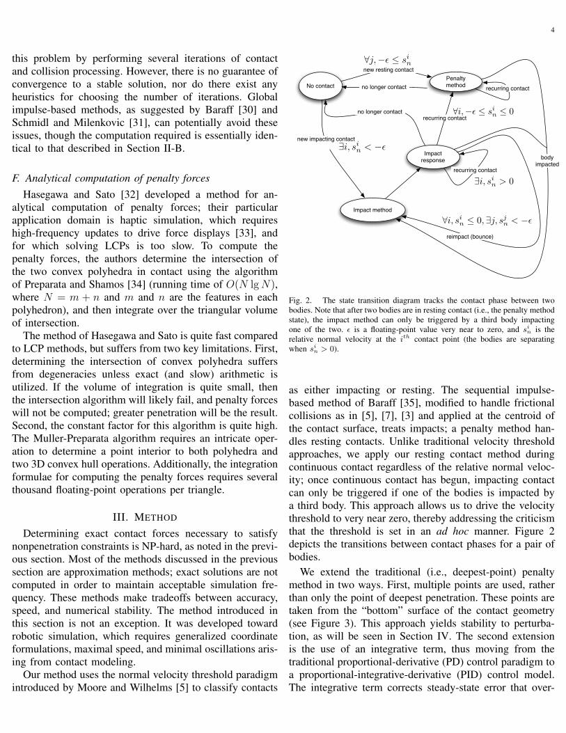
We extend the traditional (i.e., deepest-point) penaltymethod in two ways. First, multiple points are used, ratherthan only the point of deepest penetration. These points aretaken from the “bottom” surface of the contact geometry(see Figure 3). This approach yields stability to perturba-tion, as will be seen in Section IV. The second extensionis the use of an integrative term, thus moving from thetraditional proportional-derivative (PD) control paradigm toa proportional-integrative-derivative (PID) control model.The integrative term corrects steady-state error that over-

5

whelms the proportional term; practically, this means thatstacks of objects can be simulated without extensivelytweaking the PD gains.

Fig. 3. The result of the application of restoring forces to multiple pointsof penetration (in the manner of the algorithm described in this article) onsuccessive simulation steps. After a small period of time, the cube lies flat onthe planar surface and experiences little oscillation.

Given points of contact and a normal (a robust method tocompute these is given in Appendix I), computing penaltyforces requires two steps: determining the contact pointson the bottom of the volume of penetration and calculatingrestorative forces. These steps are described Sections III-A and III-B. This section concludes with a discussion ontuning gains.

A. Determining the points on the bottom of the volume ofpenetration

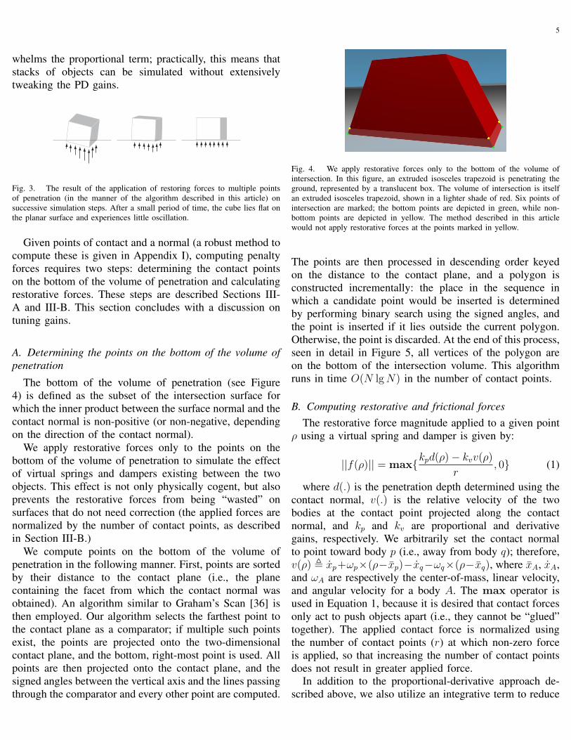
The bottom of the volume of penetration (see Figure4) is defined as the subset of the intersection surface forwhich the inner product between the surface normal and thecontact normal is non-positive (or non-negative, dependingon the direction of the contact normal).

We apply restorative forces only to the points on thebottom of the volume of penetration to simulate the effectof virtual springs and dampers existing between the twoobjects. This effect is not only physically cogent, but alsoprevents the restorative forces from being “wasted” onsurfaces that do not need correction (the applied forces arenormalized by the number of contact points, as describedin Section III-B.)

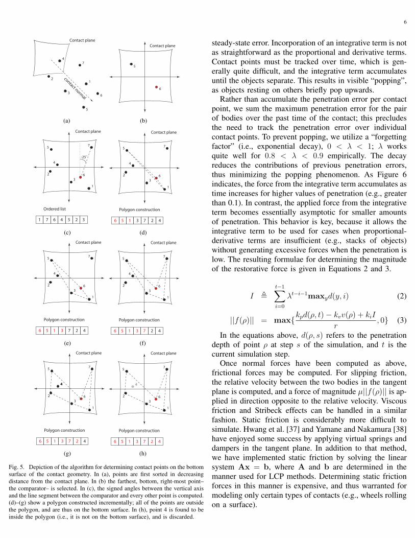
We compute points on the bottom of the volume ofpenetration in the following manner. First, points are sortedby their distance to the contact plane (i.e., the planecontaining the facet from which the contact normal wasobtained). An algorithm similar to Graham’s Scan [36] isthen employed. Our algorithm selects the farthest point tothe contact plane as a comparator; if multiple such pointsexist, the points are projected onto the two-dimensionalcontact plane, and the bottom, right-most point is used. Allpoints are then projected onto the contact plane, and thesigned angles between the vertical axis and the lines passingthrough the comparator and every other point are computed.

Fig. 4. We apply restorative forces only to the bottom of the volume ofintersection. In this figure, an extruded isosceles trapezoid is penetrating theground, represented by a translucent box. The volume of intersection is itselfan extruded isosceles trapezoid, shown in a lighter shade of red. Six points ofintersection are marked; the bottom points are depicted in green, while non-bottom points are depicted in yellow. The method described in this articlewould not apply restorative forces at the points marked in yellow.

The points are then processed in descending order keyedon the distance to the contact plane, and a polygon isconstructed incrementally: the place in the sequence inwhich a candidate point would be inserted is determinedby performing binary search using the signed angles, andthe point is inserted if it lies outside the current polygon.Otherwise, the point is discarded. At the end of this process,seen in detail in Figure 5, all vertices of the polygon areon the bottom of the intersection volume. This algorithmruns in time O(N lg N) in the number of contact points.

B. Computing restorative and frictional forcesThe restorative force magnitude applied to a given point

ρ using a virtual spring and damper is given by:

||f(ρ)|| = max{kpd(ρ)− kvv(ρ)

r, 0} (1)

where d(.) is the penetration depth determined using thecontact normal, v(.) is the relative velocity of the twobodies at the contact point projected along the contactnormal, and kp and kv are proportional and derivativegains, respectively. We arbitrarily set the contact normalto point toward body p (i.e., away from body q); therefore,v(ρ) , xp+ωp×(ρ−xp)−xq−ωq×(ρ−xq), where xA, xA,and ωA are respectively the center-of-mass, linear velocity,and angular velocity for a body A. The max operator isused in Equation 1, because it is desired that contact forcesonly act to push objects apart (i.e., they cannot be “glued”together). The applied contact force is normalized usingthe number of contact points (r) at which non-zero forceis applied, so that increasing the number of contact pointsdoes not result in greater applied force.

In addition to the proportional-derivative approach de-scribed above, we also utilize an integrative term to reduce

6

(a) (b)

(c) (d)

(e) (f)

(g) (h)

Fig. 5. Depiction of the algorithm for determining contact points on the bottomsurface of the contact geometry. In (a), points are first sorted in decreasingdistance from the contact plane. In (b) the farthest, bottom, right-most point–the comparator– is selected. In (c), the signed angles between the vertical axisand the line segment between the comparator and every other point is computed.(d)–(g) show a polygon constructed incrementally; all of the points are outsidethe polygon, and are thus on the bottom surface. In (h), point 4 is found to beinside the polygon (i.e., it is not on the bottom surface), and is discarded.

steady-state error. Incorporation of an integrative term is notas straightforward as the proportional and derivative terms.Contact points must be tracked over time, which is gen-erally quite difficult, and the integrative term accumulatesuntil the objects separate. This results in visible “popping”,as objects resting on others briefly pop upwards.

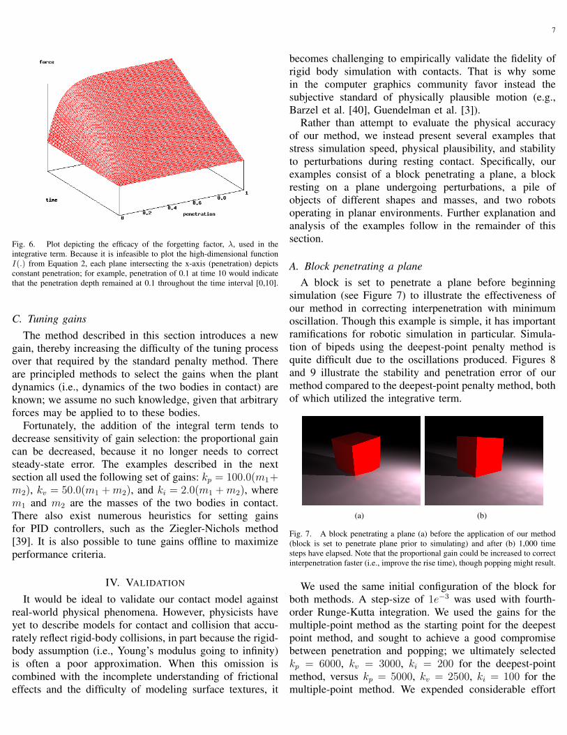
Rather than accumulate the penetration error per contactpoint, we sum the maximum penetration error for the pairof bodies over the past time of the contact; this precludesthe need to track the penetration error over individualcontact points. To prevent popping, we utilize a “forgettingfactor” (i.e., exponential decay), 0 < λ < 1; λ worksquite well for 0.8 < λ < 0.9 empirically. The decayreduces the contributions of previous penetration errors,thus minimizing the popping phenomenon. As Figure 6indicates, the force from the integrative term accumulates astime increases for higher values of penetration (e.g., greaterthan 0.1). In contrast, the applied force from the integrativeterm becomes essentially asymptotic for smaller amountsof penetration. This behavior is key, because it allows theintegrative term to be used for cases when proportional-derivative terms are insufficient (e.g., stacks of objects)without generating excessive forces when the penetration islow. The resulting formulae for determining the magnitudeof the restorative force is given in Equations 2 and 3.

I ,t−1∑i=0

λt−i−1maxyd(y, i) (2)

||f(ρ)|| = max{kpd(ρ, t)− kvv(ρ) + kiI

r, 0} (3)

In the equations above, d(ρ, s) refers to the penetrationdepth of point ρ at step s of the simulation, and t is thecurrent simulation step.

Once normal forces have been computed as above,frictional forces may be computed. For slipping friction,the relative velocity between the two bodies in the tangentplane is computed, and a force of magnitude µ||f(ρ)|| is ap-plied in direction opposite to the relative velocity. Viscousfriction and Stribeck effects can be handled in a similarfashion. Static friction is considerably more difficult tosimulate. Hwang et al. [37] and Yamane and Nakamura [38]have enjoyed some success by applying virtual springs anddampers in the tangent plane. In addition to that method,we have implemented static friction by solving the linearsystem Ax = b, where A and b are determined in themanner used for LCP methods. Determining static frictionforces in this manner is expensive, and thus warranted formodeling only certain types of contacts (e.g., wheels rollingon a surface).

7

Fig. 6. Plot depicting the efficacy of the forgetting factor, λ, used in theintegrative term. Because it is infeasible to plot the high-dimensional functionI(.) from Equation 2, each plane intersecting the x-axis (penetration) depictsconstant penetration; for example, penetration of 0.1 at time 10 would indicatethat the penetration depth remained at 0.1 throughout the time interval [0,10].

C. Tuning gainsThe method described in this section introduces a new

gain, thereby increasing the difficulty of the tuning processover that required by the standard penalty method. Thereare principled methods to select the gains when the plantdynamics (i.e., dynamics of the two bodies in contact) areknown; we assume no such knowledge, given that arbitraryforces may be applied to to these bodies.

Fortunately, the addition of the integral term tends todecrease sensitivity of gain selection: the proportional gaincan be decreased, because it no longer needs to correctsteady-state error. The examples described in the nextsection all used the following set of gains: kp = 100.0(m1+m2), kv = 50.0(m1 + m2), and ki = 2.0(m1 + m2), wherem1 and m2 are the masses of the two bodies in contact.There also exist numerous heuristics for setting gainsfor PID controllers, such as the Ziegler-Nichols method[39]. It is also possible to tune gains offline to maximizeperformance criteria.

IV. VALIDATION

It would be ideal to validate our contact model againstreal-world physical phenomena. However, physicists haveyet to describe models for contact and collision that accu-rately reflect rigid-body collisions, in part because the rigid-body assumption (i.e., Young’s modulus going to infinity)is often a poor approximation. When this omission iscombined with the incomplete understanding of frictionaleffects and the difficulty of modeling surface textures, it

becomes challenging to empirically validate the fidelity ofrigid body simulation with contacts. That is why somein the computer graphics community favor instead thesubjective standard of physically plausible motion (e.g.,Barzel et al. [40], Guendelman et al. [3]).

Rather than attempt to evaluate the physical accuracyof our method, we instead present several examples thatstress simulation speed, physical plausibility, and stabilityto perturbations during resting contact. Specifically, ourexamples consist of a block penetrating a plane, a blockresting on a plane undergoing perturbations, a pile ofobjects of different shapes and masses, and two robotsoperating in planar environments. Further explanation andanalysis of the examples follow in the remainder of thissection.

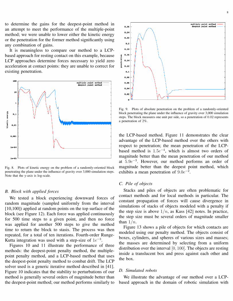
A. Block penetrating a planeA block is set to penetrate a plane before beginning

simulation (see Figure 7) to illustrate the effectiveness ofour method in correcting interpenetration with minimumoscillation. Though this example is simple, it has importantramifications for robotic simulation in particular. Simula-tion of bipeds using the deepest-point penalty method isquite difficult due to the oscillations produced. Figures 8and 9 illustrate the stability and penetration error of ourmethod compared to the deepest-point penalty method, bothof which utilized the integrative term.

(a) (b)

Fig. 7. A block penetrating a plane (a) before the application of our method(block is set to penetrate plane prior to simulating) and after (b) 1,000 timesteps have elapsed. Note that the proportional gain could be increased to correctinterpenetration faster (i.e., improve the rise time), though popping might result.

We used the same initial configuration of the block forboth methods. A step-size of 1e−3 was used with fourth-order Runge-Kutta integration. We used the gains for themultiple-point method as the starting point for the deepestpoint method, and sought to achieve a good compromisebetween penetration and popping; we ultimately selectedkp = 6000, kv = 3000, ki = 200 for the deepest-pointmethod, versus kp = 5000, kv = 2500, ki = 100 for themultiple-point method. We expended considerable effort

8

to determine the gains for the deepest-point method inan attempt to meet the performance of the multiple-pointmethod; we were unable to lower either the kinetic energyor the penetration for the former method significantly usingany combination of gains.

It is meaningless to compare our method to a LCP-based approach for resting contact on this example, becauseLCP approaches determine forces necessary to yield zeroacceleration at contact points: they are unable to correct forexisting penetration.

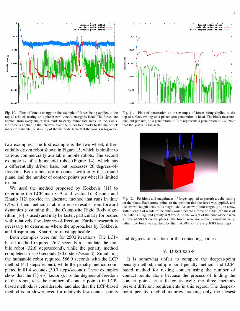
Fig. 8. Plots of kinetic energy on the problem of a randomly-oriented blockpenetrating the plane under the influence of gravity over 3,000 simulation steps.Note that the y-axis is log-scale.

B. Block with applied forcesWe tested a block experiencing downward forces of

random magnitude (sampled uniformly from the interval[10,100]) applied at random points on the top surface of theblock (see Figure 12). Each force was applied continuouslyfor 500 time steps to a given point, and then no forcewas applied for another 500 steps to give the methodtime to return the block to stasis. The process was thenrepeated, for a total of ten iterations. Fourth-order Runge-Kutta integration was used with a step-size of 1e−3.

Figures 10 and 11 illustrate the performance of threemethods: the deepest-point penalty method, the multiple-point penalty method, and a LCP-based method that usesthe deepest-point penalty method to combat drift. The LCPsolver used is a generic iterative method described in [41].Figure 10 indicates that the stability to perturbations of ourmethod is generally several orders of magnitude better thanthe deepest-point method; our method performs similarly to

Fig. 9. Plots of absolute penetration on the problem of a randomly-orientedblock penetrating the plane under the influence of gravity over 3,000 simulationsteps. The block measures one unit per side, so a penetration of 0.02 representsa penetration of 2%.

the LCP-based method. Figure 11 demonstrates the clearadvantage of the LCP-based method over the others withrespect to penetration; the mean penetration of the LCP-based method is 1.5e−4, which is almost two orders ofmagnitude better than the mean penetration of our methodat 5.9e−3. However, our method performs an order ofmagnitude better than the deepest point method, whichexhibits a mean penetration of 9.0e−2.

C. Pile of objectsStacks and piles of objects are often problematic for

contact methods and for local methods in particular. Theconstant propagation of forces will cause divergence insimulations of stacks of objects modeled with a penalty ifthe step size is above 1/n, as Kass [42] notes. In practice,the step size must be several orders of magnitude smallerthan 1/n.

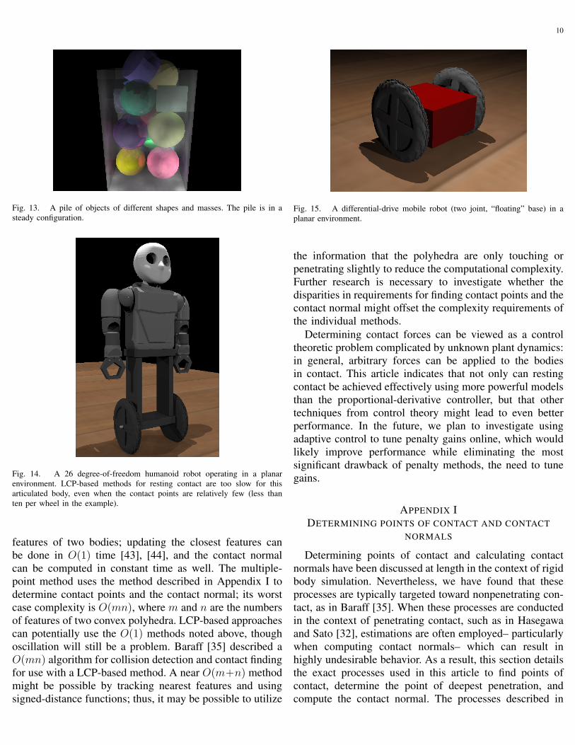
Figure 13 shows a pile of objects for which contacts aremodeled using our penalty method. The objects consist ofboxes, cylinders, and spheres of various sizes and masses;the masses are determined by selecting from a uniformdistribution over the interval [0, 100]. The objects are restinginside a translucent box and press against each other andthe box.

D. Simulated robotsWe illustrate the advantage of our method over a LCP-

based approach in the domain of robotic simulation with

9

Fig. 10. Plots of kinetic energy on the example of forces being applied to thetop of a block resting on a plane; zero kinetic energy is ideal. The forces areapplied from every major tick mark to every minor tick mark on the x-axis.No force is applied in the intervals from the minor tick marks to the major tickmarks to illustrate the stability of the methods. Note that the y-axis is log-scale.

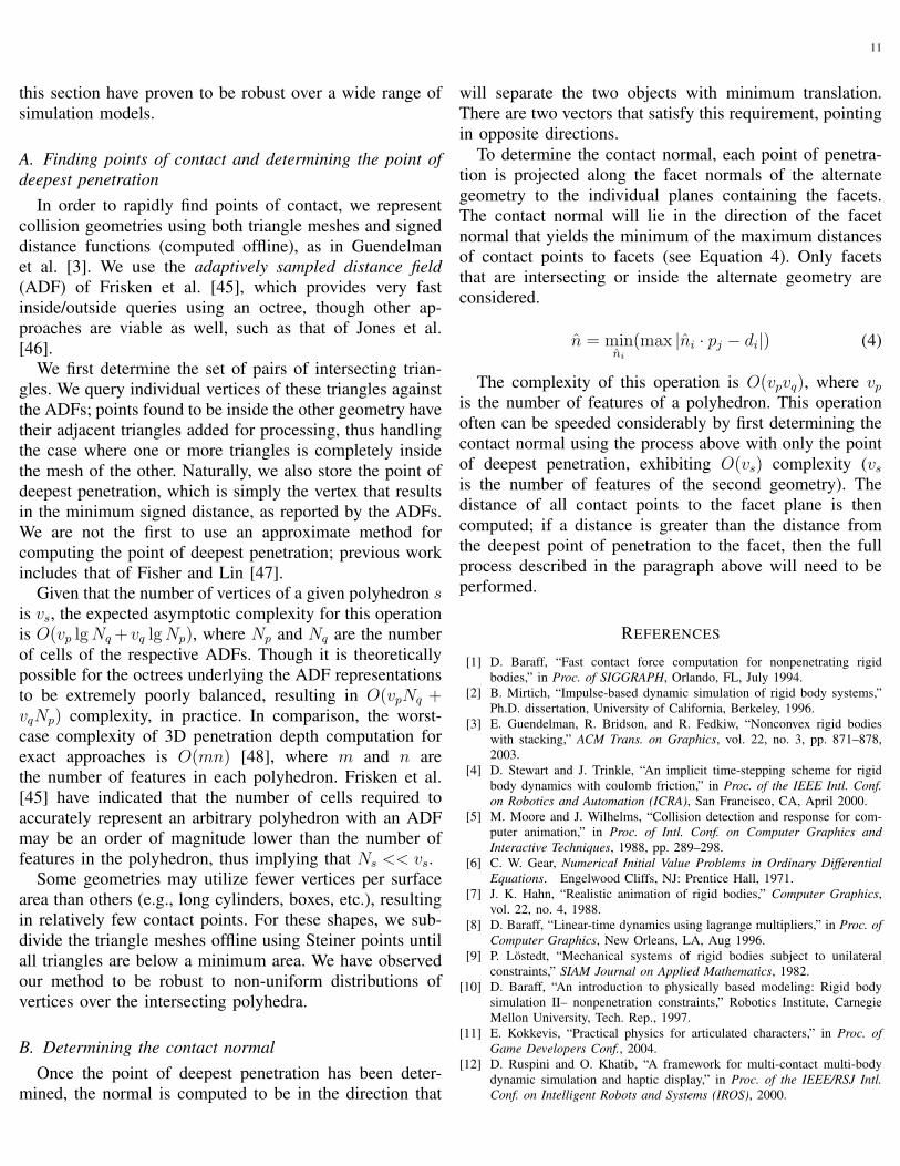
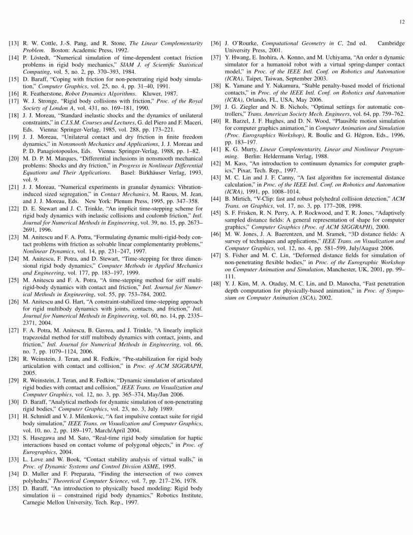
two examples. The first example is the two-wheel, differ-entially driven robot shown in Figure 15, which is similar tovarious commercially available mobile robots. The secondexample is of a humanoid robot (Figure 14), which hasa differentially driven base, but possesses 26 degrees-of-freedom. Both robots are in contact with only the groundplane, and the number of contact points per wheel is limitedto ten.

We used the method proposed by Kokkevis [11] todetermine the LCP matrix A and vector b. Ruspini andKhatib [12] provide an alternate method that runs in timeO(m3); their method is able to reuse results from forwarddynamics (assuming that the Composite Rigid Body algo-rithm [16] is used) and may be faster, particularly for bodieswith relatively few degrees-of-freedom. Further research isnecessary to determine where the approaches by Kokkevisand Ruspini and Khatib are most applicable.

Both examples were run for 2500 iterations. The LCP-based method required 76.7 seconds to simulate the mo-bile robot (32.6 steps/second), while the penalty methodcompleted in 31.0 seconds (80.6 steps/second). Simulatingthe humanoid robot required 566.9 seconds with the LCPmethod (4.4 steps/second), while the penalty method com-pleted in 81.4 seconds (30.7 steps/second). These examplesshow that the O(mn) factor (m is the degrees-of-freedomof the robot, n is the number of contact points) in LCP-based methods is considerable, and also that the LCP-basedmethod is far slower, even for relatively few contact points

Fig. 11. Plots of penetration on the example of forces being applied to thetop of a block resting on a plane; zero penetration is ideal. The block measuresone unit per side, so a penetration of 0.02 represents a penetration of 2%. Notethat the y-axis is log-scale.

Fig. 12. Positions and magnitudes of forces applied to perturb a cube restingon the plane. Each arrow points to the position that the force was applied, andthe arrow’s length denotes its magnitude. An arrow of unit length (i.e., an arrowwith a length of a side of the cube) would denote a force of 100N (the mass ofthe cube is 10kg, and gravity is 9.8m/s2, so the weight of the cube alone exertsa force of 98.1N on the plane). The forces were not applied simultaneously;rather, one force was applied for the first 500 out of every 1000 time steps.

and degrees-of-freedom in the contacting bodies.

V. DISCUSSION

It is somewhat unfair to compare the deepest-pointpenalty method, multiple-point penalty method, and LCP-based method for resting contact using the number ofcontact points alone because the process of finding thecontact points is a factor as well; the three methodspresent different requirements in this regard. The deepest-point penalty method requires tracking only the closest

10

Fig. 13. A pile of objects of different shapes and masses. The pile is in asteady configuration.

Fig. 14. A 26 degree-of-freedom humanoid robot operating in a planarenvironment. LCP-based methods for resting contact are too slow for thisarticulated body, even when the contact points are relatively few (less thanten per wheel in the example).

features of two bodies; updating the closest features canbe done in O(1) time [43], [44], and the contact normalcan be computed in constant time as well. The multiple-point method uses the method described in Appendix I todetermine contact points and the contact normal; its worstcase complexity is O(mn), where m and n are the numbersof features of two convex polyhedra. LCP-based approachescan potentially use the O(1) methods noted above, thoughoscillation will still be a problem. Baraff [35] described aO(mn) algorithm for collision detection and contact findingfor use with a LCP-based method. A near O(m+n) methodmight be possible by tracking nearest features and usingsigned-distance functions; thus, it may be possible to utilize

Fig. 15. A differential-drive mobile robot (two joint, “floating” base) in aplanar environment.

the information that the polyhedra are only touching orpenetrating slightly to reduce the computational complexity.Further research is necessary to investigate whether thedisparities in requirements for finding contact points and thecontact normal might offset the complexity requirements ofthe individual methods.

Determining contact forces can be viewed as a controltheoretic problem complicated by unknown plant dynamics:in general, arbitrary forces can be applied to the bodiesin contact. This article indicates that not only can restingcontact be achieved effectively using more powerful modelsthan the proportional-derivative controller, but that othertechniques from control theory might lead to even betterperformance. In the future, we plan to investigate usingadaptive control to tune penalty gains online, which wouldlikely improve performance while eliminating the mostsignificant drawback of penalty methods, the need to tunegains.

APPENDIX IDETERMINING POINTS OF CONTACT AND CONTACT

NORMALS

Determining points of contact and calculating contactnormals have been discussed at length in the context of rigidbody simulation. Nevertheless, we have found that theseprocesses are typically targeted toward nonpenetrating con-tact, as in Baraff [35]. When these processes are conductedin the context of penetrating contact, such as in Hasegawaand Sato [32], estimations are often employed– particularlywhen computing contact normals– which can result inhighly undesirable behavior. As a result, this section detailsthe exact processes used in this article to find points ofcontact, determine the point of deepest penetration, andcompute the contact normal. The processes described in

11

this section have proven to be robust over a wide range ofsimulation models.

A. Finding points of contact and determining the point ofdeepest penetration

In order to rapidly find points of contact, we representcollision geometries using both triangle meshes and signeddistance functions (computed offline), as in Guendelmanet al. [3]. We use the adaptively sampled distance field(ADF) of Frisken et al. [45], which provides very fastinside/outside queries using an octree, though other ap-proaches are viable as well, such as that of Jones et al.[46].

We first determine the set of pairs of intersecting trian-gles. We query individual vertices of these triangles againstthe ADFs; points found to be inside the other geometry havetheir adjacent triangles added for processing, thus handlingthe case where one or more triangles is completely insidethe mesh of the other. Naturally, we also store the point ofdeepest penetration, which is simply the vertex that resultsin the minimum signed distance, as reported by the ADFs.We are not the first to use an approximate method forcomputing the point of deepest penetration; previous workincludes that of Fisher and Lin [47].

Given that the number of vertices of a given polyhedron sis vs, the expected asymptotic complexity for this operationis O(vp lg Nq + vq lg Np), where Np and Nq are the numberof cells of the respective ADFs. Though it is theoreticallypossible for the octrees underlying the ADF representationsto be extremely poorly balanced, resulting in O(vpNq +vqNp) complexity, in practice. In comparison, the worst-case complexity of 3D penetration depth computation forexact approaches is O(mn) [48], where m and n arethe number of features in each polyhedron. Frisken et al.[45] have indicated that the number of cells required toaccurately represent an arbitrary polyhedron with an ADFmay be an order of magnitude lower than the number offeatures in the polyhedron, thus implying that Ns << vs.

Some geometries may utilize fewer vertices per surfacearea than others (e.g., long cylinders, boxes, etc.), resultingin relatively few contact points. For these shapes, we sub-divide the triangle meshes offline using Steiner points untilall triangles are below a minimum area. We have observedour method to be robust to non-uniform distributions ofvertices over the intersecting polyhedra.

B. Determining the contact normalOnce the point of deepest penetration has been deter-

mined, the normal is computed to be in the direction that

will separate the two objects with minimum translation.There are two vectors that satisfy this requirement, pointingin opposite directions.

To determine the contact normal, each point of penetra-tion is projected along the facet normals of the alternategeometry to the individual planes containing the facets.The contact normal will lie in the direction of the facetnormal that yields the minimum of the maximum distancesof contact points to facets (see Equation 4). Only facetsthat are intersecting or inside the alternate geometry areconsidered.

n = minni

(max |ni · pj − di|) (4)

The complexity of this operation is O(vpvq), where vp

is the number of features of a polyhedron. This operationoften can be speeded considerably by first determining thecontact normal using the process above with only the pointof deepest penetration, exhibiting O(vs) complexity (vs

is the number of features of the second geometry). Thedistance of all contact points to the facet plane is thencomputed; if a distance is greater than the distance fromthe deepest point of penetration to the facet, then the fullprocess described in the paragraph above will need to beperformed.

REFERENCES

[1] D. Baraff, “Fast contact force computation for nonpenetrating rigidbodies,” in Proc. of SIGGRAPH, Orlando, FL, July 1994.

[2] B. Mirtich, “Impulse-based dynamic simulation of rigid body systems,”Ph.D. dissertation, University of California, Berkeley, 1996.

[3] E. Guendelman, R. Bridson, and R. Fedkiw, “Nonconvex rigid bodieswith stacking,” ACM Trans. on Graphics, vol. 22, no. 3, pp. 871–878,2003.

[4] D. Stewart and J. Trinkle, “An implicit time-stepping scheme for rigidbody dynamics with coulomb friction,” in Proc. of the IEEE Intl. Conf.on Robotics and Automation (ICRA), San Francisco, CA, April 2000.

[5] M. Moore and J. Wilhelms, “Collision detection and response for com-puter animation,” in Proc. of Intl. Conf. on Computer Graphics andInteractive Techniques, 1988, pp. 289–298.

[6] C. W. Gear, Numerical Initial Value Problems in Ordinary DifferentialEquations. Engelwood Cliffs, NJ: Prentice Hall, 1971.

[7] J. K. Hahn, “Realistic animation of rigid bodies,” Computer Graphics,vol. 22, no. 4, 1988.

[8] D. Baraff, “Linear-time dynamics using lagrange multipliers,” in Proc. ofComputer Graphics, New Orleans, LA, Aug 1996.

[9] P. Lostedt, “Mechanical systems of rigid bodies subject to unilateralconstraints,” SIAM Journal on Applied Mathematics, 1982.

[10] D. Baraff, “An introduction to physically based modeling: Rigid bodysimulation II– nonpenetration constraints,” Robotics Institute, CarnegieMellon University, Tech. Rep., 1997.

[11] E. Kokkevis, “Practical physics for articulated characters,” in Proc. ofGame Developers Conf., 2004.

[12] D. Ruspini and O. Khatib, “A framework for multi-contact multi-bodydynamic simulation and haptic display,” in Proc. of the IEEE/RSJ Intl.Conf. on Intelligent Robots and Systems (IROS), 2000.

12

[13] R. W. Cottle, J.-S. Pang, and R. Stone, The Linear ComplementarityProblem. Boston: Academic Press, 1992.

[14] P. Lostedt, “Numerical simulation of time-dependent contact frictionproblems in rigid body mechanics,” SIAM J. of Scientific StatisticalComputing, vol. 5, no. 2, pp. 370–393, 1984.

[15] D. Baraff, “Coping with friction for non-penetrating rigid body simula-tion,” Computer Graphics, vol. 25, no. 4, pp. 31–40, 1991.

[16] R. Featherstone, Robot Dynamics Algorithms. Kluwer, 1987.[17] W. J. Stronge, “Rigid body collisions with friction,” Proc. of the Royal

Society of London A, vol. 431, no. 169–181, 1990.[18] J. J. Moreau, “Standard inelastic shocks and the dynamics of unilateral

constraints,” in C.I.S.M. Courses and Lectures, G. del Piero and F. Maceri,Eds. Vienna: Springer-Verlag, 1985, vol. 288, pp. 173–221.

[19] J. J. Moreau, “Unilateral contact and dry friction in finite freedomdynamics,” in Nonsmooth Mechanics and Applications, J. J. Moreau andP. D. Panagiotopoulos, Eds. Vienna: Springer-Verlag, 1988, pp. 1–82.

[20] M. D. P. M. Marques, “Differential inclusions in nonsmooth mechanicalproblems: Shocks and dry friction,” in Progress in Nonlinear DifferentialEquations and Their Applications. Basel: Birkhauser Verlag, 1993,vol. 9.

[21] J. J. Moreau, “Numerical experiments in granular dynamics: Vibration-induced sized segregation,” in Contact Mechanics, M. Raous, M. Jean,and J. J. Moreau, Eds. New York: Plenum Press, 1995, pp. 347–358.

[22] D. E. Stewart and J. C. Trinkle, “An implicit time-stepping scheme forrigid body dynamics with inelastic collisions and coulomb friction,” Intl.Journal for Numerical Methods in Engineering, vol. 39, no. 15, pp. 2673–2691, 1996.

[23] M. Anitescu and F. A. Potra, “Formulating dynamic multi-rigid-body con-tact problems with friction as solvable linear complementarity problems,”Nonlinear Dynamics, vol. 14, pp. 231–247, 1997.

[24] M. Anitescu, F. Potra, and D. Stewart, “Time-stepping for three dimen-sional rigid body dynamics,” Computer Methods in Applied Mechanicsand Engineering, vol. 177, pp. 183–197, 1999.

[25] M. Anitescu and F. A. Potra, “A time-stepping method for stiff multi-rigid-body dynamics with contact and friction,” Intl. Journal for Numer-ical Methods in Engineering, vol. 55, pp. 753–784, 2002.

[26] M. Anitescu and G. Hart, “A constraint-stabilized time-stepping approachfor rigid multibody dynamics with joints, contacts, and friction,” Intl.Journal for Numerical Methods in Engineering, vol. 60, no. 14, pp. 2335–2371, 2004.

[27] F. A. Potra, M. Anitescu, B. Gavrea, and J. Trinkle, “A linearly implicittrapezoidal method for stiff multibody dynamics with contact, joints, andfriction,” Intl. Journal for Numerical Methods in Engineering, vol. 66,no. 7, pp. 1079–1124, 2006.

[28] R. Weinstein, J. Teran, and R. Fedkiw, “Pre-stabilization for rigid bodyarticulation with contact and collision,” in Proc. of ACM SIGGRAPH,2005.

[29] R. Weinstein, J. Teran, and R. Fedkiw, “Dynamic simulation of articulatedrigid bodies with contact and collision,” IEEE Trans. on Visualization andComputer Graphics, vol. 12, no. 3, pp. 365–374, May/Jun 2006.

[30] D. Baraff, “Analytical methods for dynamic simulation of non-penetratingrigid bodies,” Computer Graphics, vol. 23, no. 3, July 1989.

[31] H. Schmidl and V. J. Milenkovic, “A fast impulsive contact suite for rigidbody simulation,” IEEE Trans. on Visualization and Computer Graphics,vol. 10, no. 2, pp. 189–197, March/April 2004.

[32] S. Hasegawa and M. Sato, “Real-time rigid body simulation for hapticinteractions based on contact volume of polygonal objects,” in Proc. ofEurographics, 2004.

[33] L. Love and W. Book, “Contact stability analysis of virtual walls,” inProc. of Dynamic Systems and Control Divsion ASME, 1995.

[34] D. Muller and F. Preparata, “Finding the intersection of two convexpolyhedra,” Theoretical Computer Science, vol. 7, pp. 217–236, 1978.

[35] D. Baraff, “An introduction to physically based modeling: Rigid bodysimulation ii – constrained rigid body dynamics,” Robotics Institute,Carnegie Mellon University, Tech. Rep., 1997.

[36] J. O’Rourke, Computational Geometry in C, 2nd ed. CambridgeUniversity Press, 2001.

[37] Y. Hwang, E. Inohira, A. Konno, and M. Uchiyama, “An order n dynamicsimulator for a humanoid robot with a virtual spring-damper contactmodel,” in Proc. of the IEEE Intl. Conf. on Robotics and Automation(ICRA), Taipet, Taiwan, September 2003.

[38] K. Yamane and Y. Nakamura, “Stable penalty-based model of frictionalcontacts,” in Proc. of the IEEE Intl. Conf. on Robotics and Automation(ICRA), Orlando, FL, USA, May 2006.

[39] J. G. Ziegler and N. B. Nichols, “Optimal settings for automatic con-trollers,” Trans. American Society Mech. Engineers, vol. 64, pp. 759–762.

[40] R. Barzel, J. F. Hughes, and D. N. Wood, “Plausible motion simulationfor computer graphics animation,” in Computer Animation and Simulation(Proc. Eurographics Workshop), R. Boulic and G. Hegron, Eds., 1996,pp. 183–197.

[41] K. G. Murty, Linear Complementarity, Linear and Nonlinear Program-ming. Berlin: Heldermann Verlag, 1988.

[42] M. Kass, “An introduction to continuum dynamics for computer graph-ics,” Pixar, Tech. Rep., 1997.

[43] M. C. Lin and J. F. Canny, “A fast algorithm for incremental distancecalculation,” in Proc. of the IEEE Intl. Conf. on Robotics and Automation(ICRA), 1991, pp. 1008–1014.

[44] B. Mirtich, “V-Clip: fast and robust polyhedral collision detection,” ACMTrans. on Graphics, vol. 17, no. 3, pp. 177–208, 1998.

[45] S. F. Frisken, R. N. Perry, A. P. Rockwood, and T. R. Jones, “Adaptivelysampled distance fields: A general representation of shape for computergraphics,” Computer Graphics (Proc. of ACM SIGGRAPH), 2000.

[46] M. W. Jones, J. A. Baerentzen, and M. Sramek, “3D distance fields: Asurvey of techniques and applications,” IEEE Trans. on Visualization andComputer Graphics, vol. 12, no. 4, pp. 581–599, July/August 2006.

[47] S. Fisher and M. C. Lin, “Deformed distance fields for simulation ofnon-penetrating flexible bodies,” in Proc. of the Eurographic Workshopon Computer Animation and Simulation, Manchester, UK, 2001, pp. 99–111.

[48] Y. J. Kim, M. A. Otaduy, M. C. Lin, and D. Manocha, “Fast penetrationdepth computation for physically-based animation,” in Proc. of Sympo-sium on Computer Animation (SCA), 2002.