A Fast Power Network Optimization Algorithm for Improving

A Fast Power Network Optimization Algorithm for Improving Dynamic IR-drop

Speaker: Yang-Tai KungDep. of EE, National Cheng Kung University

IntroductionProblem FormulationOverview of Our MethodologyDiscovery of Representative Power Consumption FilesPower Network Optimization AlgorithmExperimental ResultsConclusion

Outline

2


Outline

3

Powerplanning becomes a more critical step.A modern chip consumes more power when its design complexity continually increases.A design has a small margin for voltage drop as technology process advances.

Most of previous works only consider static power consumption without handling dynamic power consumption during powerplanningor power network optimization.

For simplicity, existing studies either adopt the worst or average power consumption when dynamic IR-drop is considered.

However, it may waste unnecessary routing resource if they adopt the worst power consumption to perform voltage analysis. It still has chance to violate the IR-drop or EM constraints if they adopt the average power consumption.

Introduction

4

Power network optimization considering dynamic IR-drop is very difficult and is very time consuming without a good strategy.

Power consumption of a device may be various at different time and it is composed of a large number of Power consumption Files (PFs for short) during a period of time.It is impossible to optimize power network according to all PFs.

There exist limited researches about power network optimization for dynamic IR-drop.

An efficient and effective power optimization approach to consider dynamic IR-drop is required by industry.

Introduction

5

Optimize power network according to critical PFs selected from a large set of PFs.

Apply K-clustering algorithm to classify all PFs into several groups according to power distribution maps (PDMs for short) induced by different PFs .Generate a representative power consumption file (RPF for short) for each group to represent the PFs in the group.

Propose an efficient and effective approach to repair voltage violations in the hotspot region of power network which are induced by many PFs.

The experimental results have shown that the ratio of IR-drop violations can be significantly reduced by our methodology compared to the classic approach.

Our Contributions

6


Outline

7

Input:Locations and shapes of standard cells and macros from DEF and LEF files.The average power consumption of standard cells and macros from PTPX (primetime).The capacitances of pins and wires and the power network of the chip extracted from IC Compiler.Switching activity information from RTL Value Change Dump (VCD for short).

Output: The widths of vertical power stripes (VPSs for short).

Constraints:The IR-drop constraintThe maximum current density (EM) constraintThe minimum width constraintThe maximum width constraint

Problem Formulation

8


Outline

9

Overview of Our Methodology

10

Generate PFs according to PrimeTime and VCD file, where the switching power of cells are estimated from signal switching information in a VCD file for all time slots.

𝑃𝑃𝑠𝑠𝑠𝑠𝑠𝑠𝑠𝑠𝑠𝑠𝑠𝑠𝑠𝑠𝑠𝑠𝑠 = 12∗ 𝐶𝐶 ∗ 𝑉𝑉2

Total switching power consumption at each time slot.

Time

DEF/LEF/VCD

Generate all power consumption files (PFs) from VCD

Construct power distribution maps

Eliminate non-critical power consumption files

Discover representative power consumption files (RPFs)

Optimize power network according to RPFs

Time Scale(ps)

Tota

l Pow

er C

onsu

mpt

ion(

W)


11

Eliminate non-critical PFs.A PF is not critical when its total power consumption is smaller than average power consumption.

Non-critical power consumption files.

Time Scale (ps)

Tota

l Pow

er C

onsu

mpt

ion

(W)

5.8608 5.86082 5.86084 5.86086 5.86088 5.8609 5.86092 5.86094 5.86096

2

1.8

1.6

1.4

1.2

1

0.8

0.6

0.4

0.2

0

DEF/LEF/VCD







12

PF f1 PF f2 PF f3

Each PF

Build PDMs for the critical PFs.A map is composed of ℎ grids.A PDM for a PF 𝑓𝑓𝑠𝑠 is represented by a vector 𝑋𝑋𝑠𝑠= <𝑥𝑥1𝑠𝑠 , 𝑥𝑥2𝑠𝑠 , … 𝑥𝑥𝑠𝑠𝑠 >, where 𝑥𝑥𝑗𝑗𝑠𝑠 denotes power consumption in a grid 𝑗𝑗 .

DEF/LEF/VCD







13

Classify PFs into different clusters according to their power distributions, and then select a RPF for each cluster.

Time 1~NClustering algorithm

Cluster 1 Cluster 2 Cluster 3 Cluster 4

DEF/LEF/VCD







14

DEF/LEF/VCD

Generate all power consumption files from a VCD file





Construct a voltage violation map (VVM for short) for a PF, where each grid 𝑔𝑔 corresponds to a node in a power network.

Positive value in a grid denotes the IR-drop violation value of a node; otherwise, the value is zero.

0.2 0.3 0.1 0.1 0.1

0.3 0.3 0.2 0.2 0.2

0.3 0.4 0.6 0.3 0.5

0.1 0.1 0.3 0.3 0.4

0.1 0.3 0.4 0.3 0.2

Construct a VVM for a PF

15

Construct VVMs for RPFs

Optimized P/G Network

Repeatedly select a critical RPF to optimize power network until the power network has no IR-drop violation for all RPFs.

Optimize Power Network by Selection of

a Critical RPF

YES

NO

Any IR-Drop Violation?Update VVMs for

RPFs


DEF/LEF/VCD






IntroductionProblem FormulationOverview of Our MethodologyDiscovery of Representative Power Consumption Files

Correlation MetricK-Clustering AlgorithmCost Function for a RPF in Each Group

Power Network Optimization AlgorithmExperimental ResultsConclusion

Outline

16

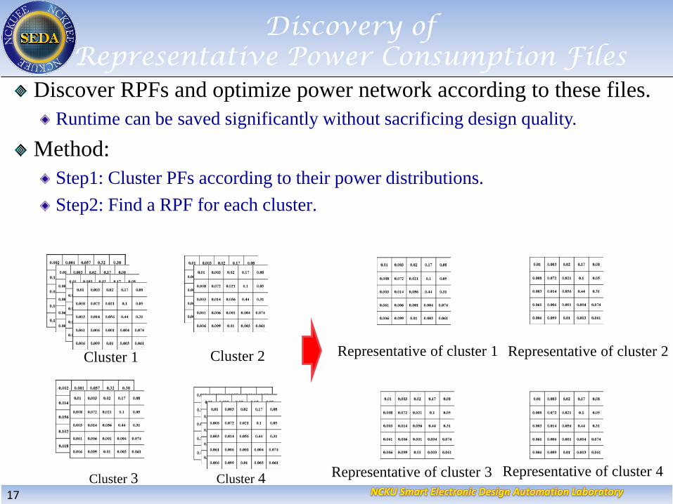
Discover RPFs and optimize power network according to these files.Runtime can be saved significantly without sacrificing design quality.

Method:Step1: Cluster PFs according to their power distributions.Step2: Find a RPF for each cluster.

Discovery of Representative Power Consumption Files

17Cluster 3

Cluster 1 Cluster 2 Representative of cluster 1 Representative of cluster 2

Representative of cluster 3 Representative of cluster 4Cluster 4

We use distance 𝑑𝑑𝑠𝑠,𝑗𝑗 to represent the similarity between PDMs 𝑋𝑋𝑠𝑠and 𝑋𝑋𝑗𝑗 of two PFs 𝑓𝑓𝑠𝑠 and 𝑓𝑓𝑗𝑗, which is calculated by the following function:

where 𝜌𝜌𝑠𝑠,𝑗𝑗 is called as statistical correlation, which is defined as follows:

where 𝜎𝜎𝑠𝑠 (𝜎𝜎𝑗𝑗) is standard deviation.

function cov(𝑖𝑖, 𝑗𝑗) represents the covariance of PDMs 𝑋𝑋𝑠𝑠 and 𝑋𝑋𝑗𝑗 as follows:

�̅�𝑥𝑠𝑠(�̅�𝑥𝑗𝑗) denotes the average power consumption in the vector 𝑋𝑋𝑠𝑠(𝑋𝑋𝑗𝑗).h denotes the number of bins in a PDM.

18

𝜌𝜌𝑠𝑠,𝑗𝑗 = 𝑠𝑠𝑐𝑐𝑐𝑐(𝑠𝑠,𝑗𝑗)𝜎𝜎𝑖𝑖 . 𝜎𝜎𝑗𝑗

, -1 ≤ 𝜌𝜌 ≤ 1

𝑑𝑑𝑠𝑠,𝑗𝑗 = 1 - 𝜌𝜌𝑠𝑠,𝑗𝑗 , 0 ≤ 𝑑𝑑𝑠𝑠,𝑗𝑗≤ 2

Correlation Metric

cov(𝑖𝑖, 𝑗𝑗) =1ℎ∗ �

𝑏𝑏=1

𝑠𝑥𝑥𝑏𝑏𝑠𝑠 − �̅�𝑥𝑠𝑠 ∗ 𝑥𝑥𝑏𝑏

𝑗𝑗 − �̅�𝑥𝑗𝑗

K-Clustering Algorithm

19

Divide all PFs into K clusters according to their power distributions.PFs in each cluster have similar power distribution.

Construction of a complete graph G(N, E) before applying K cluster algorithm.

Initialize a node 𝑛𝑛𝑠𝑠 for each PF 𝑓𝑓𝑠𝑠.Connect an edge 𝑒𝑒𝑠𝑠,𝑗𝑗 for each pair of 𝑛𝑛𝑠𝑠 and 𝑛𝑛𝑗𝑗 , where 𝑑𝑑𝑠𝑠,𝑗𝑗 denote the weight of the edge.

𝑛𝑛1

𝑛𝑛3

𝑛𝑛2

𝑐𝑐1

𝑑𝑑1,2

𝑑𝑑1,3 𝑑𝑑2,3𝑛𝑛4

𝑐𝑐4

𝑛𝑛5𝑑𝑑4,5

𝑑𝑑2,4

𝑑𝑑1,4

𝑑𝑑3,4


20

In the beginning, we consider each node 𝑛𝑛𝑠𝑠 as a cluster 𝑐𝑐𝑠𝑠.The algorithm will repeatedly combine two clusters until the number of clusters is K.After a node 𝑛𝑛𝑠𝑠 is merged into a cluster, we use 𝑐𝑐𝑠𝑠 to represent the associated cluster of 𝑛𝑛𝑠𝑠 for each edge 𝑒𝑒𝑠𝑠,𝑗𝑗 for simplicity.

𝑛𝑛1

𝑛𝑛3

𝑛𝑛2

𝑐𝑐1

𝑑𝑑1,2

𝑑𝑑1,3 𝑑𝑑2,3𝑛𝑛4

𝑐𝑐4

𝑛𝑛5𝑑𝑑4,5

𝑑𝑑2,4

𝑑𝑑1,4

𝑑𝑑3,4

21

Algorithm: K-Clustering AlgorithmInput: a weighted complete graph G(N, E); K is number of clusters;Output: K clusters, each cluster has the similar power consumption files;1. Sort all edges in 𝐸𝐸 in the non-decreasing order and store in 𝐿𝐿.2. 𝑆𝑆 ←{∅}; ► Let 𝑆𝑆 denote a set of edges connecting to two clusters.3. 𝜅𝜅 ← |N|; 4. for (each edge 𝑒𝑒𝑠𝑠,𝑗𝑗 in L ) do5. for (each edge 𝑒𝑒𝑝𝑝,𝑞𝑞 connecting to 𝑐𝑐𝑠𝑠 𝑎𝑎𝑛𝑛𝑑𝑑 𝑐𝑐𝑗𝑗 ) do6. 𝑆𝑆 ← 𝑆𝑆 ∪ {𝑑𝑑𝑝𝑝,𝑞𝑞};7. end for8. If (𝑑𝑑𝑠𝑠,𝑗𝑗 is the smallest value in S ) then9. 𝑐𝑐𝑠𝑠 ← 𝑐𝑐𝑠𝑠 ∪ 𝑐𝑐𝑗𝑗;10. Remove all edges 𝑆𝑆 from 𝐸𝐸;11. 𝜅𝜅 ← 𝜅𝜅 – 1;12. end if13. If (𝜅𝜅 = K) then14. break;15. end If16. 𝑆𝑆 ←{∅};17. end for


Select a RPF from each cluster |𝐶𝐶| if it has the maximum value according to the following function:

𝑥𝑥𝑏𝑏𝑠𝑠 : the power consumption of bin 𝑏𝑏 in PF 𝑓𝑓𝑠𝑠.𝛼𝛼 : the power consumption weight of user defined.𝛿𝛿𝑏𝑏: the distance of bin 𝑏𝑏 to the closest power pad.

𝑟𝑟𝑏𝑏 = {

Ψ 𝑓𝑓𝑠𝑠 = �𝑏𝑏=1

𝑠(𝛼𝛼 ∗ 𝑥𝑥𝑏𝑏𝑠𝑠 + 𝑟𝑟𝑏𝑏 ∗ 𝛿𝛿𝑏𝑏)

Discovery of Representative Power Consumption File

22

Distance weight

𝛿𝛿𝑏𝑏𝑏𝑏power padmacro

Power stripe

1 , 𝑖𝑖𝑓𝑓 𝑥𝑥𝑏𝑏𝑠𝑠 𝑖𝑖𝑖𝑖 𝑡𝑡𝑡𝑡𝑡𝑡 η% 𝑡𝑡𝑡𝑡𝑝𝑝𝑒𝑒𝑟𝑟 𝑐𝑐𝑡𝑡𝑛𝑛𝑖𝑖𝑐𝑐𝑐𝑐𝑡𝑡𝑡𝑡𝑖𝑖𝑡𝑡𝑛𝑛 𝑖𝑖𝑛𝑛 𝑋𝑋𝑠𝑠0 , else

Power consumption


Outline

23

Power Network Optimization Algorithm

24

YES

NO

Optimization of a Power Network According to the Selected RPF

Identification of a Hotspot Region for Each RPF

Power Network Output

Initialization of VVMs for RPFs

Optimization of a Power Network According to RPFs

Selection of the RPF with the Most Severe Hotspot Region

Fast Update of VVMs for all RPFs

Any IR-Drop Violation?

Initialization of Voltage Violation Maps for RPFs

25

YES

NO









Identification of a Hotspot Region for Each RPP

26

YES

NO









27


(a) RPF 1 Hotspot Region

0.2 0.3 0.1 0.1 0.1

0.3 0.3 0.2 0.2 0.2

0.3 0.4 0.6 0.3 0.5

0.1 0.1 0.3 0.3 0.4

0.1 0.3 0.4 0.3 0.2

0.1 0.3 0.1 0.3 0.2

0.4 0.2 0.5 0.2 0.2

0.3 0.8 0.3 0.3 0.5

0.7 0.1 0.2 0.4 0.2

0.1 0.3 0.4 0.3 0.1

0.1 0.3 0.1 0.2 0.2

0.4 0.3 0.2 0.2 0.2

0.2 0.2 0.6 0.5 0.6

0.1 0.3 0.9 0.5 0.2

0.3 0.7 0.4 0.7 0.2

0.1 0.1 0.6 0.7 0.3

0.2 0.3 0.3 0.8 0.6

0.2 0.5 0.7 0.6 0.5

0.3 0.4 0.1 0.3 0.2

0.1 0.2 0.2 0.2 0.1

VVM of RPFs 1~r

Discover the grid with the most serious IR-drop violation for each RPF.Generate a window with a proper size to cover the grid.

(b) RPF 2 Hotspot Region (c) RPF 3 Hotspot Region (d) RPF 4 Hotspot Region

Selection of RPF with the Most Serious IR-drop Region

28

YES

NO









29

Selection of RPF with the Most Severe IR-drop Region

0.23 0.62 0.45 0.29 0.14

0.32 0.68 0.52 0.21 0.54

0.29 0.44 0.61 0.24 0.40

0.19 0.18 0.38 0.30 0.39

0.16 0.34 0.24 0.13 0.37

(a) IR-drop Violation Region of RPF1

0.23 0.30 0.15 0.15 0.10

0.30 0.32 0.23 0.23 0.20

0.30 0.44 0.59 0.34 0.50

0.18 0.18 0.75 0.30 0.45

0.15 0.38 0.44 0.32 0.23

(b) IR-drop Violation Region of RPF2

0.23 0.22 0.15 0.51 0.21

0.40 0.31 0.38 0.61 0.42

0.21 0.34 0.62 0.81 0.71

0.41 0.11 0.44 0.37 0.76

0.49 0.23 0.27 0.14 0.13

(c) IR-drop Violation Region of RPF3

Select a RPF to optimize power network according to the hotspot regions in different RPFs fi’s.Use the following function to determine the priority of a fi:

𝑣𝑣𝑠𝑠𝑠𝑠 denotes IR-drop violation value of grid 𝑔𝑔 in a RPF 𝑓𝑓𝑠𝑠 .

𝜑𝜑𝑠𝑠 = �1, 𝜎𝜎 ≤ 110, 1 < 𝜎𝜎 ≤ 3100, 𝜎𝜎 > 3

, violation grid 𝑔𝑔 repeatedly appears in the window of 𝜎𝜎 RPFs.

The red region means violation repeatedly in the different RPFs.

Ψ 𝑓𝑓𝑠𝑠 = �𝑠𝑠=1

𝑠𝜑𝜑𝑠𝑠 ∗ 𝑣𝑣𝑠𝑠𝑠𝑠


30

YES

NO









Propose an iterative method to adjust the widths and lengths of VPSs in a region as follows:

Compute the equivalent VPS resistance of the regionwith the worst voltage violation, and compute the IR-drop violation ratio for each power stripe in the region.Fix the width of each VPS to a larger ESW (effective stripe width) with respect to the current width ESW in the table constructed in advance.Adjust length of VPSs according to its

equivalent resistance and IR-drop ratio.

VPSs Sizing

31


32

YES

NO

Optimization of Power Network According to the Selected RPF





Selection of the RPF with the Worst Hotspot Region



Fast Voltage Update

33

Apply an efficient node based approach to update voltages of those nodes which are close to 𝑛𝑛𝑡𝑡𝑑𝑑𝑒𝑒𝑠𝑠 if we increase the VPS area at 𝑛𝑛𝑡𝑡𝑑𝑑𝑒𝑒𝑠𝑠 .

It is quite time consuming to update the voltage of the entire power network.The computation can be limited to a small region because the change at 𝑛𝑛𝑡𝑡𝑑𝑑𝑒𝑒𝑠𝑠will propagate out and vanish after some distance.


Outline

34

Programming Language C++

Linux WorkstationCPU Intel® Xeon® E5500 2.27GHz

Memory 90GBSystem Cent OS 5.1

Environments:

Our benchmarks are based on real designs from Himax.

Experimental Results

35

Cir. # of Cells # of Mac. Supply Voltage (V) Static Power (W) Max. Power (W)

Cir1 672952 222 1.10 0.033 0.0789

Cir2 193688 277 0.81 0.503 0.7802

Cir3 5909306 874 1.10 0.903 1.3270

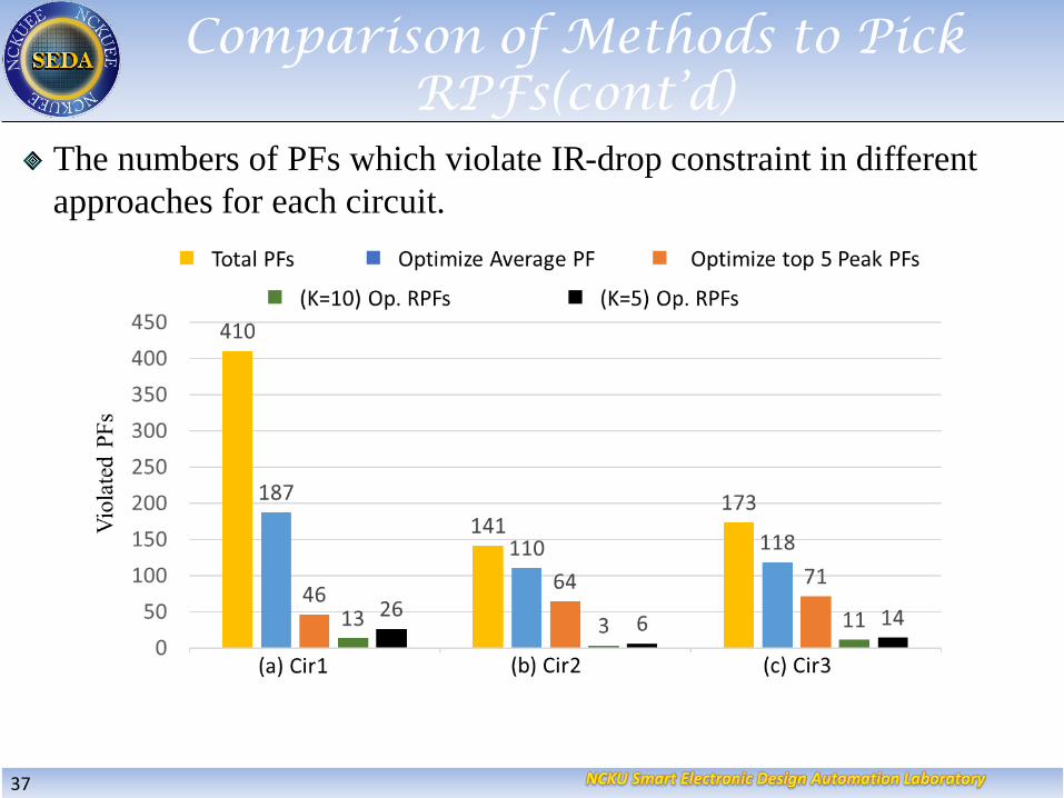
Compare with other approaches including average PF and top five worst PFs, and our K-clustering algorithm obtains the smallest “Total V.”.

“Total V.” denotes the ratios of violated PFs to the total PFs.“Total V.” by our approach are about 1/11 and 1/6 with respect to the average PF and the top five worst PF, respectively.

Comparison of Methods to Pick RPFs

36

Circuit Average PF Optimization Top Five Peak PF Optimization Selected RPF Optimization

(K = 10)

Selected RPF Optimization

(K = 5)

Area

(106

μ𝑐𝑐2)

Max

IR

drop

(mV)

Total

V.

(%)

Op.

(s)

Area

(106

μ𝑐𝑐2)

Max IR

drop

(mV)

Total V.

(%)

Op.

(s)

Area

(106

μ𝑐𝑐2 )

Max

IR

drop

(mV)

Total

V.

(%)

Cluster

(s)

Op.

(s)

Total

(s)

Area

(106

μ𝑐𝑐2)

Max

IR

drop

(mV)

Total

V.

(%)

Cluster

(s)

Op.

(s)

Total

(s)

Cir1 4.85 68.4 45.7 29 4.94 64.1 11.2 70 4.93 63.4 3.1 215 56 271 4.91 63.6 6.3 235 32 267

Cir2 25.9 49.7 78.0 48 27.8 47.3 45.3 234 27.6 46.6 2.3 190 197 387 26.6 46.3 4.2 212 140 352

Cir3 89.2 65.1 68.2 753 93.5 62.7 43.9 2672 92.2 59.3 6.3 490 2388 2878 91.9 60.1 8.1 540 1954 2494

Nor. 0.97 1.07 11.4 0.54 1.02 1.02 5.9 1.72 1.01 0.99 0.60 0.90 1.46 1.09 1.00 1.00 1.00 1.00 1.00 1.00

Comparison of Methods to Pick RPFs(cont’d)

The numbers of PFs which violate IR-drop constraint in different approaches for each circuit.

37

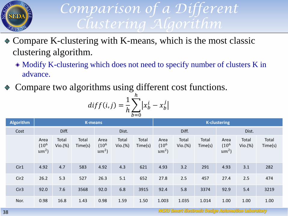
Compare K-clustering with K-means, which is the most classic clustering algorithm.

Modify K-clustering which does not need to specify number of clusters K in advance.

Compare two algorithms using different cost functions.

Comparison of a Different Clustering Algorithm

38

𝑑𝑑𝑖𝑖𝑓𝑓𝑓𝑓 𝑖𝑖, 𝑗𝑗 =1ℎ�𝑏𝑏=0

𝑠

𝑥𝑥𝑏𝑏𝑠𝑠 − 𝑥𝑥𝑏𝑏𝑗𝑗

Algorithm K-means K-clustering

Cost Diff. Dist. Diff. Dist.

Area(106𝑐𝑐𝑐𝑐2)

Total Vio.(%)

TotalTime(s)


Total Vio.(%)

TotalTime(s)


Total Vio.(%)

TotalTime(s)


Total Vio.(%)

TotalTime(s)

Cir1 4.92 4.7 583 4.92 4.3 621 4.93 3.2 291 4.93 3.1 282

Cir2 26.2 5.3 527 26.3 5.1 652 27.8 2.5 457 27.4 2.5 474

Cir3 92.0 7.6 3568 92.0 6.8 3915 92.4 5.8 3374 92.9 5.4 3219

Nor. 0.98 16.8 1.43 0.98 1.59 1.50 1.003 1.035 1.014 1.00 1.00 1.00

Compare our window based sizing algorithm with other approach including iterative methodology and sequential linear programming methodology (SLP for short) [1].

Comparison of Our Sizing Approach with Other Approaches

39

Circiut Original Status Iterative method SLP method Our method

Area(106𝑐𝑐𝑐𝑐2 )

Total OV.

Max.IR

drop(mV)


Total OV.

Max.IR

drop(mV)

Time(s)


Total OV.

Max.IR

drop(mV)

Time(s)


Total OV.

Max.IR

drop(mV)

Time(s)

Cir1 4.59 398 67.1 5.53 470 62.5 7012 4.98 440 62.9 387 4.93 423 63.4 282

Cir2 24.9 8536 52.6 35.8 40549 45.8 5221 29.1 8762 46.1 721 27.4 8682 46.7 474

Cir3 86.5 10267 66.9 137.2 14683 57.9 36850 102.6 11067 58.2 4255 92.9 10845 59.0 3219

Nor. 0.92 0.96 1.11 1.30 1.23 0.98 15.77 1.06 1.02 0.99 1.40 1.00 1.00 1.00 1.00

[1] S.S.-Y. Liu, C.-J. Lee, C.-C. Huang, H.-M. Chen, C.-T. Lin and C.-H. Lee, “Effective Power Network Prototyping Via Statistical-based Clusteringand Sequential Linear Programming,” in Proc. DATE, pp. 1701-1706, Mar. 2013.


Cluster 2

Cluster 1

Cluster 3

RPF of cluster1

40

Cluster 1 Cluster 1

Cluster 2 Cluster 2

Cluster 3Cluster 3

IR-drop of RPF1

IR-drop of RPF2

IR-drop of RPF3

RPF of cluster2

RPF of cluster3

7654321

10%9%8%7%6%5%4%3%2%1%0%

Cir 2

41


RPF1 before RPF1 after

RPF2 before

RPF3 before

RPF2 after

RPF3 after

Cir 1 Cir 2

RPF1 before RPF1 after

RPF2 before

RPF3 before

RPF2 after

RPF3 after

10%9%8%7%6%5%4%3%2%1%0%


Outline

42

Propose a power network optimization based on clustering algorithm for dynamic IR-drop.

Propose an efficient method to resolve dynamic IR-drop violations for industrial cases.

Construct PDMs from a VCD file and classify them into several categories through a clustering algorithm.Find a representative power consumption file in each cluster.Optimize power network by resizing the VPSs in the most severe voltage violation region in each RPF.

The experimental results have demonstrated that our approach can greatly reduce the ratio of violated power profiles to total critical power profiles compared to intuitive approaches.

Conclusion

43

End

44

Thank You For Your Attention

Documents

A Fast Power Network Optimization Algorithm for Improving