A Fast Projection Method for Connectivity Constraints in ...people.csail.mit.edu/stuhmer/publications/stuehmer-cremers-emmcvpr2015.pdf · Fast Projection Method for Connectivity Constraints

A Fast Projection Method forConnectivity Constraints in Image Segmentation

Jan Stuhmer and Daniel Cremers

Department of Computer Science, Technische Universitat Munchen, Germany

Abstract. We propose to solve an image segmentation problem withconnectivity constraints via projection onto the constraint set. The con-straints form a convex set and the convex image segmentation problemwith a total variation regularizer can be solved to global optimality ina primal-dual framework. Efficiency is achieved by directly computingthe update of the primal variable via a projection onto the constraintset, which results in a special quadratic programming problem similar tothe problems studied as isotonic regression methods in statistics, whichcan be solved with O(n logn) complexity. We show that especially forsegmentation problems with long range connections this method is by or-ders of magnitudes more efficient, both in iteration number and runtime,than solving the dual of the constrained optimization problem. Experi-ments validate the usefulness of connectivity constraints for segmentingthin structures such as veins and arteries in medical image analysis.

1 Introduction

To allow to preserve thin structures, topological constraints, and especially thosethat preserve connectivity [16, 15], have been introduced into image segmentationmethods.

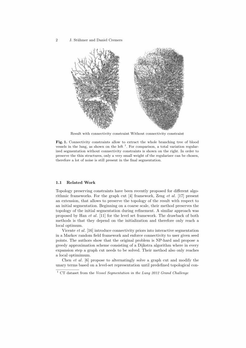
These constraints have a great advantage in several application areas, includ-ing the segmentation of arteries and veins in medical imaging but also in a userinteractive setting for general image segmentation. They are very useful whenthin structures should be extracted from image data, allowing to extract thewhole branching tree of blood vessels in the lung, as shown on the left in Fig. 1.For comparison, a total variation regularized segmentation of the dataset with-out connectivity constraints is shown on the right. In order to preserve the thinstructures, only a very small weight of the regularizer can be chosen. Thereforea lot of noise is still present in the final segmentation.

Including these constraints in the segmentation model either leads to a higheralgorithmic complexity [16, 6] or slow convergence when solving the dual of theconstrained optimization problem [15].

2 J. Stuhmer and Daniel Cremers

Result with connectivity constraint Without connectivity constraint

Fig. 1. Connectivity constraints allow to extract the whole branching tree of bloodvessels in the lung, as shown on the left 1. For comparison, a total variation regular-ized segmentation without connectivity constraints is shown on the right. In order topreserve the thin structures, only a very small weight of the regularizer can be chosen,therefore a lot of noise is still present in the final segmentation.

1.1 Related Work

Topology preserving constraints have been recently proposed for different algo-rithmic frameworks. For the graph cut [4] framework, Zeng et al . [17] presentan extension, that allows to preserve the topology of the result with respect toan initial segmentation. Beginning on a coarse scale, their method preserves thetopology of the initial segmentation during refinement. A similar approach wasproposed by Han et al . [11] for the level set framework. The drawback of bothmethods is that they depend on the initialization and therefore only reach alocal optimum.

Vicente et al . [16] introduce connectivity priors into interactive segmentationin a Markov random field framework and enforce connectivity to user given seedpoints. The authors show that the original problem is NP-hard and propose agreedy approximation scheme consisting of a Dijkstra algorithm where in everyexpansion step a graph cut needs to be solved. Their method also only reachesa local optimimum.

Chen et al . [6] propose to alternatingly solve a graph cut and modify theunary terms based on a level-set representation until predefined topological con-

1 CT dataset from the Vessel Segmentation in the Lung 2012 Grand Challenge

Fast Projection Method for Connectivity Constraints in Image Segmentation 3

straints are fulfilled. The runtime complexity of the method prevents to use itfor large scale problems.

Recently, three different methods were proposed, that aim to reach a globaloptimum. First, Nowozin and Lampert [12] propose to formulate the image seg-mentation problem with topological constraints as a linear program relaxation.However, even for small image sizes the runtime complexity of the method doesnot scale well and the relaxation is not tight. In contrast to the method presentedin this publication, their method is not suitable for large scale problems in 3Dsegmentation.

Gulshan et al . [10] introduce geodesic star shape priors into the graph cutframework. The solution of the segmentation is restricted to the shape of ageodesic star around an input seed, while the geodesic distance depends on theimage gradient. If multiple input seeds are given, the foreground segment takesthe form of a geodesic forest, the union of the geodesic stars for every seed. Adrawback of their method is that the boundary length regularizer is affected bythe discretization of the pixel neighborhood.

In a previous work [15] we propose a global optimal segmentation methodwith connectivity constraints in a convex optimization framework. The combi-nation of a total variation regularizer with a connectivity constraint allows tosegment thin structures even in very noisy image data. Compared to the workof Gulshan et al . [10] our method uses a continuous segmentation frameworkand therefore the boundary length regularizer is not biased by discretizationartifacts. The constrained optimization problem in [15] is solved by computinga solution of the dual problem. In this work, we propose an efficient projectionscheme to directly compute a solution for the update of the primal variable.

1.2 Contribution

We propose to solve an image segmentation problem with connectivity con-straints via projection onto the constraint set. We show that the constraintsform a convex set and derive a projection algorithm from isotonic regressionmethods in statistics. We show that especially for segmentation problems withlong range connections this method is by orders of magnitudes more efficient,both in iteration number and runtime, than solving the dual of the constrainedoptimization problem.

2 Connectivity Constraints in Image Segmentation

First lets review the results from [15] where image segmentation with connectiv-ity constraints is formalized as the constrained optimization problem

minu∈BV (Ω;[0,1])

∫Ω

f(x)u(x) + |∇u| dx (1)

s.t.

∀x ∈ Ω, u(x) = 1 : ∃Cxs ∈ Gs : u (Cxs (t)) = 1. C1


where I is an image with the domain Ω, a bounded connected subset of Rm,BV (Ω; [0, 1]) is the space of functions with bounded variation and f : Ω → Rdepends on the image data. The data term f is chosen in such a way that itis negative for image values which a more likely to be foreground and neg-ative in regions which should be regarded as background, e.g. the log ratio

f(x) = log P (I(x)|l(x)=0)P (I(x)|l(x)=1) . The discrete label assignment l : Ω → 0, 1, that

describes if an image region belongs to the object of interest l(x) = 1 or theimage background l(x) = 0, is relaxed by introducing the continuous indica-tor function u : Ω → [0, 1]. The total variation regularizer |∇u| measures theboundary length of the foreground segment. With Cxs we formalize the shortestgeodesic path from a given starting point s, for example defined by user input,to a terminal point x which is part of the geodesic shortest path tree Gs.

The solution of the optimization problem should satisfy the connectivityconstraint C1:

For each x ∈ Ω that belongs to the foreground there must exist a connectedshortest geodesic path from a given s ∈ Ω to x such that all p ∈ Ω in the pathbetween x and s belong to the foreground.

This constraint not only ensures the connection of every labeled foregroundregion to s but also ensures that the whole foreground segment is connected.

2.1 Geodesic Distances

Recently, shortest geodesic distance measures have been successfully applied toimage segmentation problems including medical image segmentation [3] as wellas general image segmentation[1, 7].

In order to define the geodesic shortest path tree Gs, first we have to choosean appropriate local geodesic metric. If λ = 0 the labeling function u(x) takes thevalue 1 for f(x) < 0 and 0 for f(x) > 0. We leave out the special case f(x) = 0 asit does not occur in practice. For all xp ∈ Ω that do not belong to the foregroundbut need to be added to the foreground to satisfy the connectivity constraintobviously u(xp) = 0 and therefore f(xp) ≥ 0. The optimal cost of the connectingpath between a fixed s and any x in the region that should be connected on Gsis then given by

minCx

s

∫ T

0

f+(C(t))dt, (2)

with f+ = max(0, f(x)). Thus, we choose the non negative cost funciton f+ asmetric for the construction of Gs. Thus the shortest path tree can be computedusing Djkstra’s algorithm [8].

More complex prior models for the geodesic path are possible. In [15] we couldshow that a bending energy prior for the construction of the geodesic shortestpath tree can improve the segmentation performance on a retinal blood vesseldataset to some extent.


3 Constrained Convex Optimization

The geodesic shortest path tree forms a directed acyclic graph Gs = V,E withthe set of vertices V with |V | = n and the set of directed edges E ⊂ V ×V with|E| = m. We follow [15] and formulate the global connectivity constraint as amonotonicity constraint over each edge of this graph. To satisfy the connectivityconstraint we observe that the value of the discretized value function ui of anode i with distance to the root node di should always be greater or equal thanthe labels of its neighbors with a larger distance dj > di to the root node. Thisimplies that the directional derivative

∂iuj := (du)(eij) = (u(j)− u(i))

of u at vertex i along the edge to vertex j should always be less or equal to zero.The image segmentation problem Eq. (1) thus can be written as the con-

strained optimization problem

minui[0,1]

∫Ω

f(x)u(x) + λ|∇u| dx (3)

s.t.

∂iuj ≤ 0, ∀(i, j) ∈ E.

This image segmentation problem can be optimized using the Primal-Dualframework of [14, 5] which can be applied to convex optimization problems witha saddle-point structure

minu∈U

maxp∈P〈Ku, p〉+G(u)− F ∗(p), (4)

where U and P are finite-dimensional vector spaces, K : U → P is a continuouslinear operator and G : U → [0,+∞) and F ∗ : P → [0,+∞) are proper, convex,lower semicontinuous functions. The update steps in [5] are computed using theprox-operator, which is defined as

v = (I + τ∂G)−1(u) = arg minv

||u− v||2

2τ+G(v)

. (5)

Using this prox-operator, the updates in the primal variable u and the dualvariable p are computed as

uk+1 = (I + τ∂G)−1(uk − τK∗pk+1) (6)

pk+1 = (I + σ∂F ∗)−1(pk + σK

(uk+1 + θ

(uk+1 − uk

))). (7)

To formulate the image segmentation problem Eq. (3) in the Primal-Dualframework we reformulate the total variation regularizer by introducing a dualvariable p ∈ R2 [14] and after discretization arrive at the saddle point problem

minui∈[0,1]

max|p|≤1

λ〈∇u, p〉+ 〈f, u〉+ δ≤0(∇iu), (8)


where ∇iu is the stacked vector of the directional derivatives ∂iuj and the con-nectivity constraint is included by adding its indicator function1. We identifythe function G(u) in Eq. (4) with G(u) = 〈f, u〉+ δ≤0(∇iu).

While the constraints over the domains of u and p can be solved by sim-ple projections, the optimization with respect to the connectivity constraint ismore involved. In the following, we will investigate two different strategies toincorporate the connectivity constraint.

3.1 Optimization via Fenchel Duality

In [15] we propose to optimize the dual of the constrained optimization problem

minui∈[0,1]

max|p|≤1α≥0

λ〈∇u, p〉+ 〈f, u〉+ 〈α,∇iu〉. (9)

The connectivity constraint is ensured by introducing an additional dual variableαij for each edge (i, j) ∈ E. Especially for long range connections the convergenceof these multipliers is very slow as we show in our experiments in section 4.

3.2 Projection onto the Constraint Set

In this section we describe how the connectivity constraint can be included bydirectly computing the update of the primal variable subject to this constraint.Therefore we propose an efficient projection scheme to solve the constrainedquadratic programming problem, which results from the definition of the prox-operator.

According to [5] the update in the primal variable u is defined as

uk+1 = (I + τ∂G)−1(uk + τ div pk+1) (10)

= arg minv∈[0,1]

||v − (uk + τ div pk+1)||2

2τ+ 〈f, v〉+ δ≤0(∇iv)

. (11)

By completing the square and omitting terms independent of v we arrive at

uk+1 = arg minv∈[0,1]

||v − (uk + τ div pk+1 − τf)||2 + δ≤0(∇iv)

(12)

which is of the general form

arg minvi∈[0,1]

||v − u||2 (13)

s.t.

vi ≥ vj , ∀(i, j) ∈ E,

with u = (uk + τ div pk+1 − τf).

1 Note that while ∇iu is defined on the graph Gs, the gradient ∇u used in the totalvariaton regularizer is computed using standard forward operators on the image grid.


Proposition 1. The feasible set C determined by the constraints of the opti-mization problem Eq. (13) is a convex set.

Proof. Let C1 be the feasible set determined by the inequality constraints andC2 the constraint on the range of v. The feasible set of Eq. (13) then is C =C1 ∩ C2. First we show that C1 is convex. If for every a, b ∈ C1 and α, β > 0 itholds that αa + βb ∈ C1 then C1 is a convex cone. Because a, b ∈ C1 it holdsthat

ai ≥ aj , bi ≥ bj , ∀(i, j) ∈ E, (14)

and because α, β > 0 it follows

αai ≥ αaj , βbi ≥ βbj , ∀(i, j) ∈ E, (15)

αai + βbi ≥ αaj + βbj , ∀(i, j) ∈ E. (16)

Hence the set C1 is a convex cone. In addition to the inequality constraintswe also have the constraint on the range of v. We call the feasible set of thisconstraint C2 = [0, 1]. This set is convex, so C = C1 ∩ C2, the intersection oftwo convex sets, is convex. ut

Thus the optimization problem Eq. (13) is strictly convex subject to convexconstraints. Its solution is an Euclidean projection of u onto the set C and canbe solved to global optimality. Furthermore the inequality constraints describea partial order on the values of v. A quadratic programming problem with thisstructure is known in statistics as isotonic regression [2].

3.3 Isotonic Regression on a Tree

In Pardalos et al . [13] the authors investigate a class of algorithms for isotonicregression where the constraints define a partial order which can be representedby a directed graph. In particular the authors propose an O(n log n) algorithmfor the case when the directed graph is a directed tree with n vertices. Forconvenience we present the algorithm IRT-BIN here as Algorithm 1.

We call the isotonic regression problem subject to partial order constraintsIRT. This problem does not include the range constraints of Eq. (13). In thefollowing, we will show that a projection of the optimal solution of IRT on therange constraint yields the optimal solution of Eq. (13).

First we follow the presentation of Pardalos et al . [13] and describe the al-gorithm for isotonic regression with partial order constraints, using the conceptof upper sets, lower sets and level sets:

Definition 1. Let X be a nonempty finite set. Let be a partial order on X.Let Y be a nonempty subset of X. We define the average of Y as Av(Y ) =1|Y |∑i∈Y ui. We call a subset L ⊂ X a lower set of X with respect to if

i ∈ X, j ∈ L and i j implies i ∈ L. Consequently a subset U ⊂ X is an upperset if i ∈ U , j ∈ X and i j implies j ∈ U . We call a subset S ⊂ X a level


set if there are an upper set U and a lower set L such that S = L ∪ U . A blockB of X is a nonempty level set such that for each upper set U ⊂ X for whichU ∩B 6= ∅ it holds that Av(B) ≥ Av(U ∩B).

Furthermore the authors of [13] introduce the concept of a block class:

Definition 2. A collection ∆ of blocks of X is called a block class of X if

1. the blocks in ∆ are pairwise disjoint and their union is the set X.2. the collection ∆ can be ordered by a partial-order such that A B for

A,B ∈ ∆ if there exist i ∈ A and j ∈ B such that i j.

Note that the collection of all singleton subsets x with x ∈ X is a block class.The authors prove that the optimal solution of IRT on a block B is vi =

Av(B) for every i ∈ B. Furthermore they show that if a block class ∆ has noadjacent violators, then the optimal solution of the isotonic regression is givenby v∗i = Av(B(i)), where B(i) is the block which contains i, for each element iof X.

Algorithm 1 IRT-BIN from Pardalos et al . [13]

1: Let ∆ be the singleton block class and let T be a copy of the underlying rootedtree.

2: Mark each leaf node of T as solved and all other nodes as unsolved.3: for each node xi of T do4: Create a block B(xi) = xi and a binomial heap Hi.5: end for6: if all nodes of T are marked as solved then7: output the blocks corresponding to the nodes in T as the final block class and

stop;8: end if9: Let xi be an unsolved node of T such that all the children nodes of xi are solved.

10: Let B(xi) (resp. Hi ) be the block (resp. binomial heap) corresponding to node xi.11: while Av(B(xi)) < Maximum(Hi) do12: ExtractMax(Hi) and let B(xk) be the corresponding block13: Shrink the edge connecting xi to xk . the new vertex is still called vi14: Create a new block B(xi)← B(xi) ∪B(xk) . the new block is still called

B(xi)15: Calculate the Av(B(xi)) for the new block B(xi)16: Hi ← Union(Hi, Hk) . this is the binomial heap for the new block B(xi)17: end while18: Mark the node xi of T as solved.19: Let xp be the parent node of xi in T . Let Hp be the binomial heap corre-

sponding to B(xp) and let ai be the node in Hp which corresponds to B(xi).ChangeKey(ai, Av(B(xi)), Hp).

20: go to 6.

We will show with the proof of the following proposition that given a solutionv∗ of IRT the optimal solution to Eq. (13) is achieved by projecting v∗ on C2.


Thus, we can directly project onto the constraints of the optimization problemEq. (13) by first projecting onto the isotonicity constraint and then onto the[0, 1]-box constraint.

Obviously, projecting first onto the [0, 1]-box constraint and then onto theisotonicity constraint will not lead to a valid projection. When the averagingstep is performed after the [0, 1] clipping, in case that the isotonicity constraintis violated and some values are smaller 1, only block average values well below 1can be achieved, even when the average of the block before projection was largerthan 1.

Proposition 2. Direct Projection onto the Constraint SetLet B be a block of X. Let v∗i = Av(B) for every i ∈ B be the solution of IRT.Let π[0,1] : R→ [0, 1] be a projection that projects negative values to 0 and values

larger 1 to 1. Thenπ[0,1](v

∗i ) : i ∈ B

is the optimal solution to the optimization

problem (13) on B.

Proof. Let us assume that B has m elements x1, x2, . . . , xm. We look at the threecases Av(B) > 1, Av(B) ∈ [0, 1] and Av(B) < 0. Obviously these three cases areexhaustive. If Av(B) ∈ [0, 1] then the solution v∗ of IRT also fulfills the rangeconstraint and the solution of Eq. (13) for the set B is identical to the solutionof IRT on B.

If Av(B) > 1 we follow a similar proof as in [13] and show that the pointπ[0,1](v

∗i ) : i ∈ B

=(π[0,1] (Av (B)) , π[0,1] (Av (B)) , . . . , π[0,1] (Av (B))

)∈ Rm

= (1, 1, . . . , 1) ∈ Rm (17)

is the optimal solution to Eq. (13) by showing that the inner product of thegradient of Eq. (13) with any feasible direction d ∈ Rm at that point is a non-negative number.

Let d = (d1, d2, . . . , dm) be a feasible direction of the isotonic regressionproblem on B. Then, in order to preserve isotonicity, feasibility of the directiond implies di ≤ dj when xi xj .

Therefore there exists a permutation σ = (σ(1), σ(2), . . . , σ(m)) such that

dσ(1) ≥ dσ(2) ≥ · · · ≥ dσ(m) (18)

andxσ(i) xσ(j) =⇒ i ≤ j. (19)

To prove that for Av(B) > 1 the point in (29) is the optimal solution of theoptimization problem (13) on the set B it is sufficient show that∑

i∈B(1− uσ(i))× dσ(i) ≥ 0. (20)

From Eq. (18) and from the definition of a block it follows that

1

m− k + 1

m∑i=k

uσ(i) ≥ Av(B) > 1 for all 1 < k ≤ m. (21)


This implies that

m∑i=k

(1− uσ(i)) ≤ 0 for all 1 < k ≤ m. (22)

Equations (22) and (18) imply that for all 1 < k ≤ m that the followinginequality holds

m∑i=k

(1− uσ(i))× dσ(k−1) ≥m∑i=k

(1− uσ(i))× dσ(k). (23)

Because Av(B) > 1 the feasibility of d implies that dσ(i) ≤ 0 for all i ∈1, . . . ,m. Combining everything together we get

m∑i=1

(1− uσ(i))× dσ(1) (24)

=

1∑i=1

(1− uσ(i))× dσ(i) +

m∑i=2

(1− uσ(1))× dσ(1)

≤1∑i=1

(1− uσ(i))× dσ(i) +

m∑i=2

(1− uσ(2))× dσ(2)

=

2∑i=1

(1− uσ(i))× dσ(i) +

m∑i=3

(1− uσ(2))× dσ(2)

≤2∑i=1

(1− uσ(i))× dσ(i) +

m∑i=3

(1− uσ(3))× dσ(3)

. . .

≤m∑i=1

(1− uσ(i))× dσ(i) (25)

From Av(B) > 1 it follows that

m∑i=1

(1− uσ(i)) < 0. (26)

Together with dσ(i) ≤ 0 for all i ∈ 1, . . . ,m it follows for Eq. (24)

m∑i=1

(1− uσ(i))× dσ(1) ≥ 0. (27)

Therefore from Eq. (24) to Eq. (25) we have proven that if Av(B) > 1

m∑i=1

(1− uσ(i))× dσ(i) ≥ 0. (28)


If Av(B) < 0 we have to show that the inner product of the gradient of Eq.(13) with any feasible direction d = (d1, d2, . . . , dm) ∈ Rm at the point

π[0,1](v∗i ) : i ∈ B

= (0, 0, . . . , 0) ∈ Rm

is a positive number. This proof is equivalent to the proof for Av(B) > 1. ut

4 Experimental Results

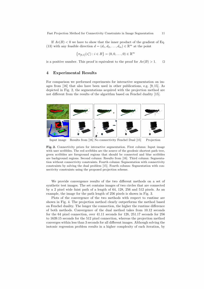
For comparison we performed experiments for interactive segmentation on im-ages from [16] that also have been used in other publications, e.g. [9, 15]. Asdepicted in Fig. 2, the segmentations acquired with the projection method arenot different from the results of the algorithm based on Fenchel duality [15].

Input image Results from [16] No connectivity Fenchel Dual [15] Projection

Fig. 2. Connectivity priors for interactive segmentation. First column: Input imagewith user scribbles. The red scribbles are the source of the geodesic shortest path tree,green scribbles are foreground regions that should be connected and blue scribblesare background regions. Second column: Results from [16]. Third column: Segmenta-tion without connectivity constraints. Fourth column: Segmentation with connectivityconstraints by solving the dual problem [15]. Fourth column: Segmentation with con-nectivity constraints using the proposed projection scheme.

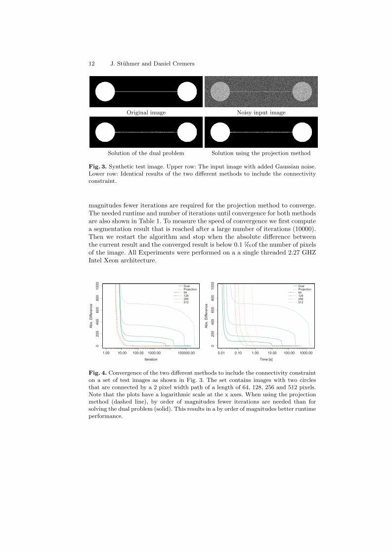
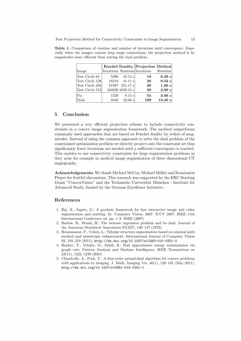
We provide convergence results of the two different methods on a set ofsynthetic test images. The set contains images of two circles that are connectedby a 2 pixel wide faint path of a length of 64, 128, 256 and 512 pixels. As anexample, the image for the path length of 256 pixels is shown in Fig. 3.

Plots of the convergence of the two methods with respect to runtime areshown in Fig. 4. The projection method clearly outperforms the method basedon Fenchel duality. The longer the connection, the higher the runtime differenceof both methods. Convergence of the dual method takes from 10.12 secondsfor the 64 pixel connection, over 41.11 seconds for 128, 251.17 seconds for 256to 1639.15 seconds for the 512 pixel connection, whereas the projection methodconverges within less than 3 seconds for all different images. Although solving theisotonic regression problem results in a higher complexity of each iteration, by


Original image Noisy input image

Solution of the dual problem Solution using the projection method

Fig. 3. Synthetic test image. Upper row: The input image with added Gaussian noise.Lower row: Identical results of the two different methods to include the connectivityconstraint.

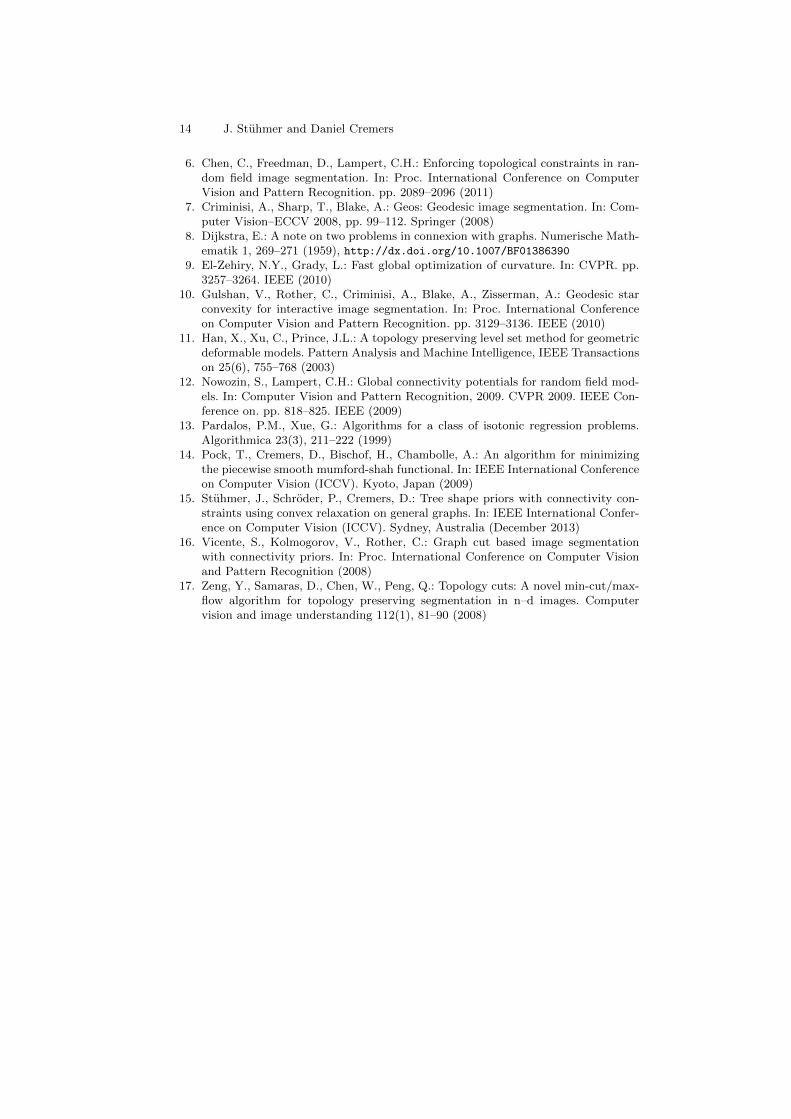
magnitudes fewer iterations are required for the projection method to converge.The needed runtime and number of iterations until convergence for both methodsare also shown in Table 1. To measure the speed of convergence we first computea segmentation result that is reached after a large number of iterations (10000).Then we restart the algorithm and stop when the absolute difference betweenthe current result and the converged result is below 0.1of the number of pixelsof the image. All Experiments were performed on a a single threaded 2.27 GHZIntel Xeon architecture.

0200

400

600

800

1000

Iteration

Abs. D

iffe

rence

1.00 10.00 100.00 1000.00 100000.00

DualProjection64128256512

0200

400

600

800

1000

Time [s]

Abs. D

iffe

rence

0.01 0.10 1.00 10.00 100.00 1000.00

DualProjection64128256512

Fig. 4. Convergence of the two different methods to include the connectivity constrainton a set of test images as shown in Fig. 3. The set contains images with two circlesthat are connected by a 2 pixel width path of a length of 64, 128, 256 and 512 pixels.Note that the plots have a logarithmic scale at the x axes. When using the projectionmethod (dashed line), by order of magnitudes fewer iterations are needed than forsolving the dual problem (solid). This results in a by order of magnitudes better runtimeperformance.


Table 1. Comparison of runtime and number of iterations until convergence. Espe-cially when the images contain long range connections, the projection method is bymagnitudes more efficient than solving the dual problem.

Fenchel Duality Projection MethodImage Iterations Runtime Iterations Runtime

Test Circle 64 5396 10.12 s 19 0.29 sTest Circle 128 18318 41.11 s 20 0.52 sTest Circle 256 81987 251.17 s 20 1.06 sTest Circle 512 344030 1639.15 s 20 2.89 s

Fly 1226 9.13 s 54 3.66 sDesk 3440 42.00 s 109 13.40 s

5 Conclusion

We presented a very efficient projection scheme to include connectivity con-straints in a convex image segmentation framework. The method outperformscommonly used approaches that are based on Fenchel duality by orders of mag-nitudes. Instead of using the common approach to solve the dual problem of theconstrained optimization problem we directly project onto the constraint set thussignificantly fewer iterations are needed until a sufficient convergence is reached.This enables to use connectivity constraints for large segmentation problems asthey arise for example in medical image segmentation of three dimensional CTangiography.

Acknowledgements We thank Michael McCoy, Michael Moller and KonstantinPieper for fruitful discussions. This research was supported by the ERC StartingGrant ”ConvexVision” and the Technische Universitat Munchen - Institute forAdvanced Study, funded by the German Excellence Initiative.

References

1. Bai, X., Sapiro, G.: A geodesic framework for fast interactive image and videosegmentation and matting. In: Computer Vision, 2007. ICCV 2007. IEEE 11thInternational Conference on. pp. 1–8. IEEE (2007)

2. Barlow, R., Brunk, H.: The isotonic regression problem and its dual. Journal ofthe American Statistical Association 67(337), 140–147 (1972)

3. Benmansour, F., Cohen, L.: Tubular structure segmentation based on minimal pathmethod and anisotropic enhancement. International Journal of Computer Vision92, 192–210 (2011), http://dx.doi.org/10.1007/s11263-010-0331-0

4. Boykov, Y., Veksler, O., Zabih, R.: Fast approximate energy minimization viagraph cuts. Pattern Analysis and Machine Intelligence, IEEE Transactions on23(11), 1222–1239 (2001)

5. Chambolle, A., Pock, T.: A first-order primal-dual algorithm for convex problemswith applications to imaging. J. Math. Imaging Vis. 40(1), 120–145 (May 2011),http://dx.doi.org/10.1007/s10851-010-0251-1


6. Chen, C., Freedman, D., Lampert, C.H.: Enforcing topological constraints in ran-dom field image segmentation. In: Proc. International Conference on ComputerVision and Pattern Recognition. pp. 2089–2096 (2011)

7. Criminisi, A., Sharp, T., Blake, A.: Geos: Geodesic image segmentation. In: Com-puter Vision–ECCV 2008, pp. 99–112. Springer (2008)

8. Dijkstra, E.: A note on two problems in connexion with graphs. Numerische Math-ematik 1, 269–271 (1959), http://dx.doi.org/10.1007/BF01386390

9. El-Zehiry, N.Y., Grady, L.: Fast global optimization of curvature. In: CVPR. pp.3257–3264. IEEE (2010)

10. Gulshan, V., Rother, C., Criminisi, A., Blake, A., Zisserman, A.: Geodesic starconvexity for interactive image segmentation. In: Proc. International Conferenceon Computer Vision and Pattern Recognition. pp. 3129–3136. IEEE (2010)

11. Han, X., Xu, C., Prince, J.L.: A topology preserving level set method for geometricdeformable models. Pattern Analysis and Machine Intelligence, IEEE Transactionson 25(6), 755–768 (2003)

12. Nowozin, S., Lampert, C.H.: Global connectivity potentials for random field mod-els. In: Computer Vision and Pattern Recognition, 2009. CVPR 2009. IEEE Con-ference on. pp. 818–825. IEEE (2009)

13. Pardalos, P.M., Xue, G.: Algorithms for a class of isotonic regression problems.Algorithmica 23(3), 211–222 (1999)

14. Pock, T., Cremers, D., Bischof, H., Chambolle, A.: An algorithm for minimizingthe piecewise smooth mumford-shah functional. In: IEEE International Conferenceon Computer Vision (ICCV). Kyoto, Japan (2009)

15. Stuhmer, J., Schroder, P., Cremers, D.: Tree shape priors with connectivity con-straints using convex relaxation on general graphs. In: IEEE International Confer-ence on Computer Vision (ICCV). Sydney, Australia (December 2013)

16. Vicente, S., Kolmogorov, V., Rother, C.: Graph cut based image segmentationwith connectivity priors. In: Proc. International Conference on Computer Visionand Pattern Recognition (2008)

17. Zeng, Y., Samaras, D., Chen, W., Peng, Q.: Topology cuts: A novel min-cut/max-flow algorithm for topology preserving segmentation in n–d images. Computervision and image understanding 112(1), 81–90 (2008)

Documents

A Fast Projection Method for Connectivity Constraints in ...people.csail.mit.edu/stuhmer/publications/stuehmer-cremers-emmcvpr2015.pdf · Fast Projection Method for Connectivity Constraints