Embed Size (px)
Citation preview
Portland State University Portland State University
PDXScholar PDXScholar
Dissertations and Theses Dissertations and Theses
1979
A feasibility analysis of a directly sun-pumped A feasibility analysis of a directly sun-pumped
carbon dioxide laser in space carbon dioxide laser in space
Seiichi Morimoto Portland State University
Follow this and additional works at: https://pdxscholar.library.pdx.edu/open_access_etds
Part of the Materials Science and Engineering Commons
Let us know how access to this document benefits you.
Recommended Citation Recommended Citation Morimoto, Seiichi, "A feasibility analysis of a directly sun-pumped carbon dioxide laser in space" (1979). Dissertations and Theses. Paper 2798. https://doi.org/10.15760/etd.2794
This Thesis is brought to you for free and open access. It has been accepted for inclusion in Dissertations and Theses by an authorized administrator of PDXScholar. Please contact us if we can make this document more accessible: [email protected].
I
AN ABSTRACT OF THE THESIS OF Seiichi Morimoto for the Mast.er of
Science in Applied Science presented May 17, 1979.
Title: A Feasibility Analysis of a Directly Sun-Pumped Carbon
Dioxide Laser in Space.
APPROVED BY MEMBERS OF THE THESIS COMMITTEE:
GeOrgeTSODgaS ,
~M. Heneghan
Selmo Taub
The possibility of using sunlight to pump a CW carbon dioxide laser
has been analyzed. Such a laser could be of interest for such applica-
tions as space communication and power transmission. In order to
optically pump co2 using sunlight, the intense vibrational-rotational
absorption bands of co2
in the 4.3 micron spectral region would have
to be utilized. The total pumping power from sunlight can be calculated
from the known data of the solar spectral irradiance outside the
atmosphere and the infrared absorption by carbon dioxide at 4.3
microns. The pumping power is proportional to the collector area of
the sunlight and is also dependent on the characteristics of the
absorbing gas mixture, such as the gas composition, the gas tempera-
ture, the total pressure of the mixture, the partial pressure of
co2
, and the. absorption path length of the sunlight in the gas.
To analyze the carbon dioxide laser system, a thermodynamic
approach was used with a simplified co2
chemical kinetic model. The
gain and saturation intensity were obtained by solving a set of
2
energy balance equations which describe the processes among the various
vibrational modes. From those results, along with the estimated cavity
losses, the output power was found.
Initially, the computation was carried out for a co2-He mixture
for the total pressure range 0.01-0.05 atm with various concentrations
of co2
at temperatures of 200°K and 300°K, and with the following
system parameters specified: a tube of 100 cm length and 1.7 cm
2 diameter, pumping from one end, 1% residual losses, and a 10 m col-
lector. All the collected sunlight was assumed to enter the cavity
without losses. Then the parameters were varied to examine their
influence on the results. 2
The 10 m collector and a 2 m absorption
path length were found to be necessary to achieve sufficient gain and
high output power. While the performance was found to be quite sensi-
tive to a number of the individual parameters, the net effect was that
the optimum output was obtained under conditions which are close to
those initially set. The optimum performance at 200°K was obtained
at 0.02 atm total pressure with 50% co2
; then the gain was about 5%/m
and the output power was about 250 milliwatts. The corresponding
efficiency of converting absorbed pump light into laser output was
about 4%. At 300°K the gain was found to be unacceptably low because
the lower laser level was more highly populated. Thus, the gas must be
cooled to achieve sufficient gain. At total pressures above about
0.05 atm the··small signal gain was too low, while at pressures below
0.01 atm the gain and output power decreased on account of the low
input power and diffusion e_ffects. Therefore, this particular type
of co2 laser would not appear to be capable of operation at pressures
above atmospheric where continuous tunability can be achieved.
This preliminary analysis indicates that it should be feasible
to directly sun-pump a carbon dioxide laser in space. The laser would
be a modest power, low gain system compared with the demonstrated
sun-pumped Nd:YAG laser. If co2
output is required or desirable for
any of a number of reasons, then this study indicates that direct sun
pumping is possible.
3
·.
A FEASIBILITY ANALYSIS OF A DIRECTLY
SUN-PUMPED CARBON DIOXIDE LASER IN SPACE
by
SEIICHI MORIMOTO
A thesis submitted in partial fulfillment of the requirements for the degree of
MASTER OF SCIENCE in
APPLIED SCIENCE
Portland State University
1979
TO THE OFFICE OF GRADUATE STUDIES AND RESEARCH:
The members of the Committee approve the thesis of
Seiichi Morimoto presentad May -17, 1979.
Selmo Tauber
APPROVED:
Terrence Wil~s; Mechanieal Engineering Section Head, Department of Engineering and Applied Science
Graduate StudieS and Research
ACKNOWLEDGEMENTS
The author wishes t? express his sincere appreciation to
Dr. George Tsongas for his invaluable guidance and unending
assistance throughout the course of this study. In addition,
his kind and patient contribution of so much time and effort to
improve my writing is gratefully appreciated.
It is also a pleasure to acknowledge Dr. Gail Massey of
the Oregon Graduate Center and Dr. Walter Christiansen and Dr.
Oktay Yesil of the University of Washington for fruitful
discussions and helpful suggestions.
_J
TABLE OF CONTENTS
PAGE
ACKNOWLEDGEMENTS · iii
LIST OF FIGURES vi
NOMENCLATURE viii
1. INTRODUCTION 1
2. FEASIBILITY ANALYSIS · 4
2.1 SOLAR POWER OUTSIDE THE ATMOSPHERE AND ITS
ABSORPTION BY co2 MOLECULES 4
2.2 THEORETICAL MODEL AND CHEMICAL KINETICS OF
CARBON DIOXIDE 10
2.2.1 Vibrational Energy Levels · · · · · · · · 10
2.2.2 Rotational Energy Levels 14
2.2.3. Vibrational Relaxation· 16
2. 3 PREDICTION OF GAIN AND POWER OUTPUT · 22
2.3.1 Minimum Pumping Power Required for
Population Inversion 22
2.3.2 Gain Coefficient 23
2.3.3 Energy Balance Equations 28
2.3.4 Saturation Intensity and the Maximum
Available Power ... 30
2.3.5 Cavity Losses and Output Coupling 31
2.3.6 Threshold Gain and Output Power 32
v
3. RESULTS AND DISCUSSION ...... . . .... 34
35
3.1 PROPOSED LASER SYSTEM MODEL
3.1.1 Description of the System ..... 35
3.1. 2 Computed Results for Proposed Laser . . 36
3.2 EFFECTS OF PARAMETER VARIATION ON THE SMALL SIGNAL.
40 GAIN AND· THE OUTPUT POWER. . . .
3.3. PRACTICAL DESIGN CONSIDERATIONS .• 47
4. CON CL US IONS . . . . . . . . . . . . . . . . . . . . . . . . . . 49
REFERENCES· . · . · . . . . . · . . . . . . . . . . . . . . . . . . 51
LIST OF FIGURES
FIGURE PAGE
1. The Infrared Absorptivity of co2 in the 4.3 Micron
Region at 200°K for Various Total Pressures
and co2
Partial Pressures for a 2 Meter Absorpt-ion
Path Length . .
2. Segmentation of the Absorptivity Curve for Calculation
of Total Pumping Power
3. Total Pumping Power at 200°K for a 10 m 2 Collector and
a 2 Meter Absorption Path Length.
Total Pumping Power at 300°K for a 10 m 2 Collector and 4.
a 2 Meter Absorption Path Length ...
5. Partial Energy Level Diagram for Carbon Dioxide
6. Temperature. Dependence of Relaxation Lifetime of
(010) Level . . . . . . . . . . . . . . . . . . . . . . .
7. Temperature Dependence of Relaxation Lifetime of
(001) Level . . . .
8. Simplified Energy Level Diagram
9. Net Generated Power per Unit Volume Versus Intensity .
10. Variation of Small Signal Gain with Total and Partial
Pressures ..................
6
7
8
9
11
20
21
28
31
37
vii
LIST OF FIGURES (Cont'd)
FIGURE PAGE
11. Variation of Output Power with Total and Partial
Pressures . 39
12. Output Power Versus Residual Loss at 200°K . 42
13. Output Power and Small Signal Gain Versus Sun Collector
Area· at 200°K ... 43
14. Output Power and Small Signal Gain Versus Beam Radius
................ ... 45
15. Output Power and Small Signal Gain Versus Absorption 0
Path Length at 2qo K ...... . . .. 46
16. Schematic Diagram of a Sun-pumped co2
Laser with End-
pumping . . . . . ...... 47
English:
A
A m
A s
B
c
D
E v
E v
I
NOMENCLATURE
-1 Einstein A coefficient, sec
2 Cross-sectional area of the beam, cm
2 Area of the sun collector, cm
-1 Rotational constant, cm
-1 Velocity of light, cm•sec
The mean relative velocity of co2
and the species
-1 k (C for co
2 and H for He), m•sec
. ff . 2 -1 Di usion constant, cm •torr•sec
Vibrational per unit volume, -3
energy J•cm
Vibrational in equilibrium, -3
energy J•cm
Vibrational of symmetric mode, -3 energy J•cm
-3 Vibrational energy of bending mode, J•cm
-3 Vibrational energy of asymmetric mode, J•cm
-3 Combined vibrational energy of E
1 and E
2, J•cm
Lineshape function, sec
Degeneracy of J-th rotational level
Degeneracy of lower vibrational level
Degeneracy of upper vibrational level
Planck's constant = 6.626 x l0-34 J•sec
-2 Intensity of light, watts•cm
-2 Intensity of incident light, watts•cm
English:
I s
i
J
J'
k
L
L. l.
m c
N
N. l.
NOMENCLATURE (Cont'd) '
-2 Saturation intensity, watts•cm
Vibrational quantum number
Rotational quantum number of the
Rotational quantum number of the
upper level
lower level
Boltzmann constant = 1.38 x l0-23 J•oK-1
Total intensity loss per pass, %
Residual intensity loss per pass, %
Length of the laser tube, cm
Absorption path length of the sunlight, cm
The mass of a co2
molecule, kg
The mass of a molecule of species k, kg
-3 Population density of co2
, molecules•cm
Population dnesity of species k (C for co2
, H for
-3 He), molecules•cm
Population density of the i-th vibrational level,
-3 molecules· cm
Population density of the lower vibrational level,
-3 molecules•cm
Population density of the upper vibrational level,
-3 molecules•cm
Population density of the j-th rotational level,
molecules•cm- 3
Population density of the vibrational-rotational
-3 lower level, molecules•cm
ix
English:
p max
p . min
.P e
p 0
p
p c
R
r
r m
T
T
T v
NOMENCLATURE (Cont'd)
Population density of the vibrational-rotational
upper level, molecules•cm -3
Maximum available power, watts
Minimum pumping power, watts
Cavity power (net power generated in the cavity), watts
Output power, watts
Total pumping power, watts
Solar spectral irradiance at 4.3 microns,
-2 -1 watts•cm •µ
Total pressure of the mixture, atm
Partial pressure of co2
, atm
Vibrational partition function
Vibrational partition function for symmetric mode
Vibrational partition function for bending mode
Vibrational partition function for asynunetric mode
Rotational partition function
. -3 Pumping power density, watts•cm
Radius of the laser tube, cm
Beam radius, cm
0 Translational temperature (gas temperature), K
Useful mirror transmission, %
Vibrational temperature, OK
Vibrational temperature of symmetric mode, OK
Vibrational temperature of bending mode,°K
Vibrational temperature of asymmetric mode, OK
x
_J
English:
v
v m
w
z
z
Greek:
Cl
Cl. 1
y
y 0
yt
E. 0
E • ]_
£J
n
e v
NOMENCLATURE (Cont'd)
. 1 0 Rotationa temperature, K
Spontaneous emission lifetime, sec
3 Volume of the laser tube, cm
3 Volume of the beam, cm
SyIIlll1etric stretching mode
Bending mode
Asymmetric stretching mode
I d d . . -1
n uce emmision rate, sec
The amount of co2
(product of co2
partial pressure
and absorption path length), atm•cm
The number of collisions required for deactivation
Distance, cm
Spectral absorptivity
Spectral absorptivity at a specific wavelength
Gain (gain coefficient),
11 . 1 . -1 Sma signa gain, cm
-1 Threshold gain, cm
Zero-point energy, J
-1 cm
Quantized vibrational energy of i-th state, J
Quantized rotational energy of j-th level, J
Energy conversion efficiency
Characteristic temperature for vibration, °K
Greek:
\)
\)
\) c
\) 0
CJ
CJ c-k
'['
c
'['
c-c
TC-H
'[' coll,3
NOMENCLATURE (Cont'd)
Characteristic temperature for symmetric mode (1920°K)
Characteristic temperature for bending mode (960°K)
Characteristic temperature for asymmetric mode (3380°K)
Characteristic temperature for rotation (.565°K)
Laser wavelength (-10.6µ),µ
Pumping wavelength (-4.3µ),µ
Spectral interval in wavelength,µ
Frequency, Hz
-1 Wavenumber, cm
Collision frequency,
Center frequency, Hz
Pumping frequency, Hz
sec
Spectral interval, -1
cm
Doppler linewidth, Hz
Lorenzian linewidth, Hz
-1
. 1 . 2 Optica cross section, cm
xii
Collision cross section of each species with co2 (C for
2 C0
2 and H for He), cm
Relaxation lifetime, sec
Time interval between collisions, sec
Relaxation lifetime by collision with co2
, sec
Relaxation lifetime by collision with Re, sec
Collisional relaxation lifetime of uppper laser
level, sec
xiii
NOMENCLATURE (Cont'd)
Greek:
'[ d Diffusion lifetime, sec
'[ rad Radiative lifetime, sec
'[ 1 Relaxation lifetime of lower laser level, sec
'[ 3 Relaxation lifetime of upper laser level, sec
. We Fractional concentration of co2
ljJH Fractional concentration of He
1. INTRODUCTION
At the present rate of growth, the worldwide space cormnunication
demand for new channels will be serious in the near future. The capacity
of a cormnunication channel is proportional to the width of its band of
frequencies. Thus, a laser emitting in the visible or infrared region
of the spectrum, where enormously wide bands of frequencies are available,
has the potential to carry many more times the amount of information
than radio waves or even microwaves·. This is the main reason for wanting
to use a laser, but optical cormnunication has another advantageous
feature. The spatial coherence of a laser beam makes possible highly
directional transmission unattainable by conventional radio techniques,
which allows lower transmission losses and at the same time maintains
secrecy by preventing easy interception of the signals. Moreover, in
space use laser cormnunication is not limited at all by atmospheric
scattering, absorption, and turbulence. For many of the same reasons
and others, lasers are also of interest for power transmission in space.
In view of the interest in laser cormnunication or power transmission
in space, it is natural to consider the possibility of sun-pumping a
laser since the external pumping source could possibly be eliminated.
A long lifetime and lightweight system might be possible by this pumping
approach compared.with other conventional pumping methods such as
electrical pumping using solar cells or other types of power supplies.
One of the most appropriate applications of a space-qualifi~d sun-pumped
2
laser would be on a synchronous orbiting satellite which is occluded
from the sun during only a small fraction of its orbit.
To date mostly solid state lasers have been studied for sun-
pumping: Both theoretical and experimental investigations on sun-
pumping Nd:YAG, Nd:Glass, Nd:Cawo4
, and ruby lasers have been reported. 1- 4
Among these candidates, the Nd:YAG laser seems most promising since
it is most highly excited above the threshold value for a given sun-
pumping level and hence has the highest output power. In fact, GTE
Sylvania has developed and successfully demonstrated a sun-pumped
Nd:YAG laser obtaining about two watts CW output power with a 0~3 m2
collector using an end-pumping method and conductive cooling. 5
However, for both space communication and power transmission
other types of lasers including co2
lasers have been considered. For
example, carbon dioxide lasers have several advantages for both
applications. First, they are considered to be relatively reliable
and long-lived. In addition, high temporal and spatial coherence and
outstanding frequency stability compared with solid state lasers is
expected. Moreover, C02
lasers offer a signal-to-noise advantage over
Nd:YAG lasers. 6 Since infrared lasers have a greater beam divergence
than visible lasers, their tracking systems need not be as precise.
But this fact also means co2
lasers need more power output. The critical
technology problem for a co2 laser system in space is that of providing
6 Doppler compensation in heterodyne detection systems.
Regarding the possibility of sun-pumping carbon dioxide, the co2
molecule has intense and wide vibration-rotational absorption bands in
the 4.3 micron region, among others. It is those bands that would have
to be utilized to optically pump co2
. Actually the feasibility of
achieving considerable power by optical excitation of a co2
laser
by its own radiation and also by blackbody radiation was hypothesized
- 7 8 by Bokhan. ' In fact, he experimentally proved optical pumping to
be practical by obtaining one watt of laser power for a co2
(50 Torr)
- N2(1 atm) mixture with radiation from the hot combustio.n process
of CO in oxygen providing the pump light. 9 Similar work was done
b . 10 y Wieder. 1 . 1 d h . . 11 d 12 More recent y Yesi an C ristiansen an others
have measured gain in a co2 gas mixture optically pumped by black
body radiation in an effort to demonstrate the feasibility of solar
pumping. In addition, Chang and Wood optically pumped a co2
laser
with a pulsed HBr laser and produced a peak power of a few kilo-
watts for pulses of about 2.2 nsec using extremely high pressure
(33 atm) pure co2.
However, the possibility of using the sun to directly pump co2
has not previously been pursued. Yet it would be extremely bene-
ficial to know whether such pumping is feasible, and if so to what
degree. How might its performance compare with that of the Nd:YAG
sun-pumped laser? Thus, the objective of this study is to analyze
3
the feasibility of a .directly sun-pumped co2
laser for space applica
tion. To do that, a simplified theoretical model of such a co2
laser is developed, as described in the chapters to follow.
2. FEASIBILITY ANALYSIS
2.1 SOLAR POWER OUTSIDE THE ATMOSPHERE AND ITS ABSORPTION BY co2
MOLECULES
In ord~r to determine whether a carbon dioxide laser can be pumped
using sunlight, two questions must be answered:
1. In what spectral region does carbon dioxide absorb light for
pumping?
2. Is enough sunlight available in that region to achieve suffi-
cient gain and power output, given the absorption character-
istics of co2?
As noted earlier, carbon dioxide absorbs incident light strongly in the
4.3 micron region. Thus, the amount of solar power available at that
wavelength must be determined. Although a great deal of solar spectrum
data is available for the visible region, beyond 2.4 mircons no complete
spectrum ?as been obtained outside (or inside) the atmosphere. However,
0 it is similar to that of a 6000 K gray-body and can be extrapolated from
the known data for shorter wavelengths. From a table of solar spectral
· d' d 15 d · d h 1 · d. (d f' d h irra iance ata so etermine , t e spectra irra iance e ine as t e
incident radiant energy flux per unit surface area per unit spectral
interval) outside the atmosphere for the 4.3 micron region is given as
~2 1 PA= 0.00073 watts cm µ-
With the available solar power known, the absorption of the sun-
light by carbon dioxide must be considered. The infrared absorptivity
(the fraction of the incident radiation absorbed) of carbon dioxide
at 4.3 microns has been calculated for a wide range of values of
16 17 * absorption path length, pressure, and temperature. '
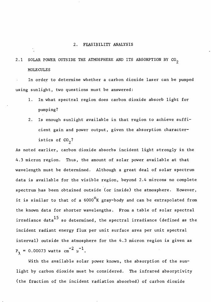
Here some typical values of the spectral absorptivity a are
plotted- in Figure 1 for various total pressures p and partial pressures
of carbon dioxide p ; the absorption path length of the sunlight i is c a
** taken to be 2 meters (round trip path in a 1 m tube is assumed).
5
Clearly, there is more absorption at high pressures where more absorbing
molecules exist. Pressures higher than those given are not presented
because they will be shown to correspond to non-optimum laser performance.
Assuming no losses transmitting the incident sunlight into the
cavity (in reality some loss factor would exist), the total solar pumping
power PT into a given cavity can be calculated from the following
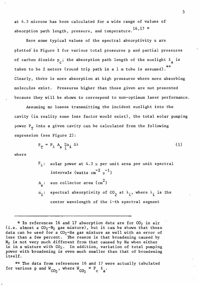
expression (see Figure 2):
where
PT = P, A L~· ~/.. I\ s l. i
P./..: solar power at 4.3 µ per unit area per unit spectral
intervals (watts cm- 2 µ-l)
A : sun collector area (cm2) s
a.: spectral absorptivity of co2 at /...' where /... is the i i i
center wavelength of the i-th spectral segment
* In references 16 and 17 absorption data are for C02 in air (i.e. almost a C02-N2 gas mixture), but it can be shown that these data can be used for a co2 -He gas mixture as well with an error of less than a few percent. The reason is that broadening caused by N2 is not very much different from that caused by He when either is in a mixture with C02. In addition, variation of total pumping power with broadening is even much smaller than that of broadening itself.
** The data from references 16 and 17 were actually tabulated for various p and WC
02, where WC
02 =Pc ia.
(1)
1
0.8
~
,.. 0.6
>1 E-l H > H E-1 P-1 ~ 0 00
0.4 ~
0.2
2250 2300 2350
WAVENUMBER,v (CM-l)
6
p =0.05 ATM p =0.025 ATM
c
ATM ATM
p =0.01 ATM p =0.005 ATM
c
2400
Figure 1. The infrared absorptivity of C02 in the 4.3 micron region at 200°K for various total pressures p and co2 partial pressures p for a 2 meter absorption path length:
c
8A: spectral interval of the given absorptivity data* (µ)
It should be noted that this procedure for the determination of PT is
used because the absorptivity data is provided in tabular form at dis-
crete wavelength intervals.
a.. tS l.
....
WAVELENGTH, A
Figure 2. Segmentation of the Absorptivity Curve for Calculation of PT.
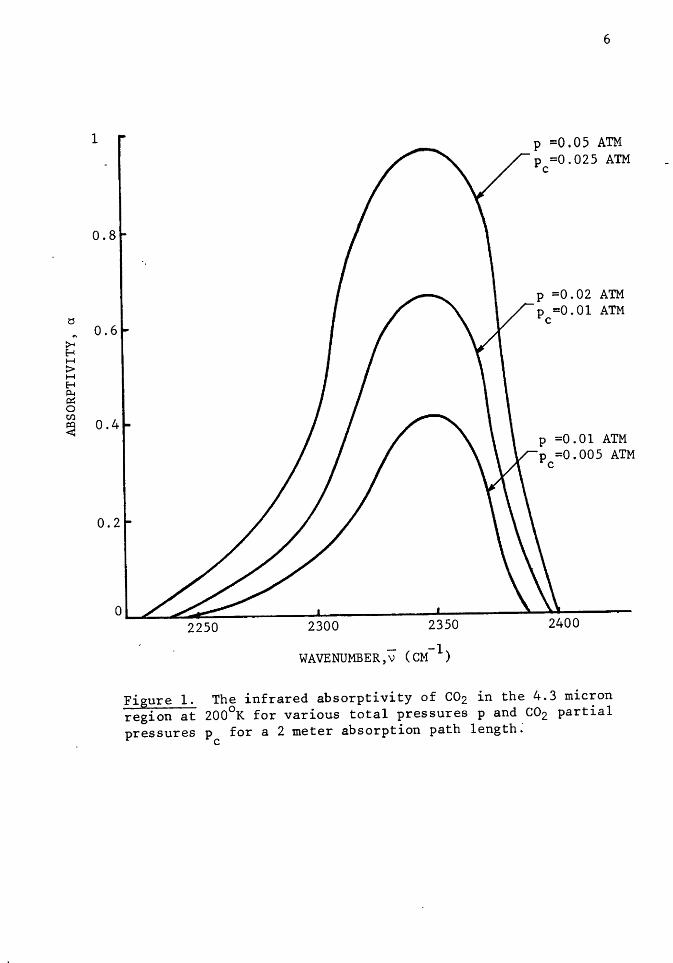
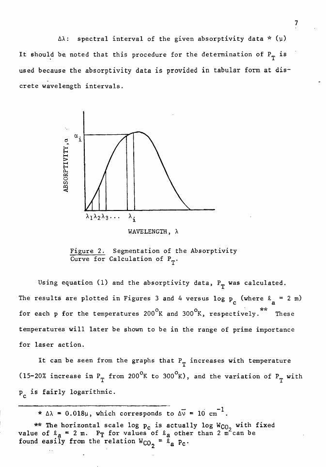
Using equation (1) and the absorptivity data, PT was calculated.
7
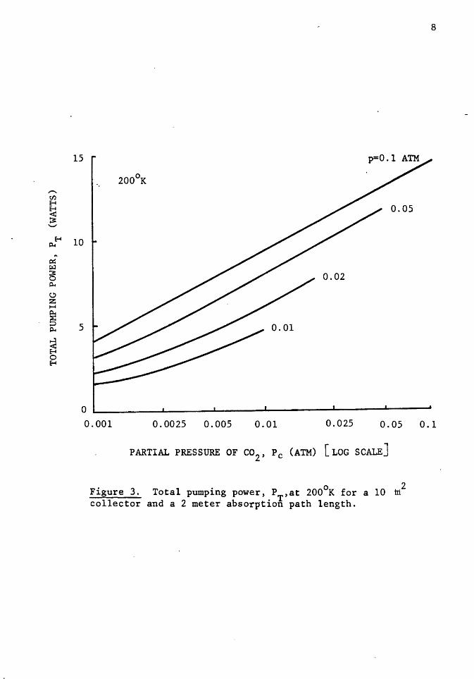
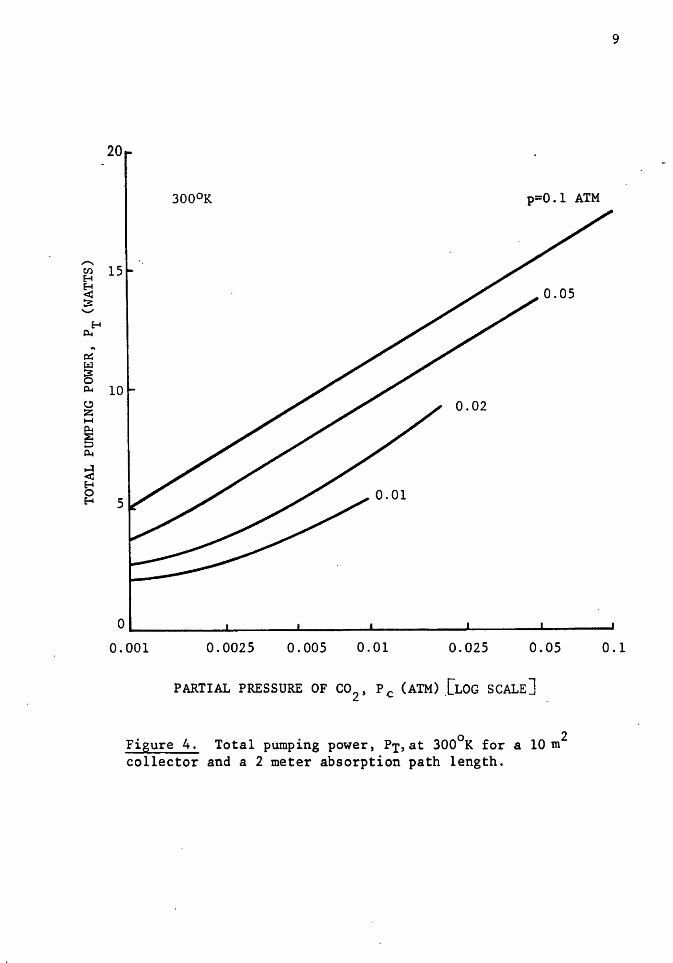
The results are plotted in Figures 3 and 4 versus log p (where ~ = 2 m) c a
0 0 . ** for each p for the temperatures 200 K and 300 K, respectively. These
temperatures will later be shown to be in the range of prime importance
for laser action.
It can be seen from the graphs that PT increases with temperature
(15-20% increase in PT from 200°K to 300°K), and the variation of PT with
p is fairly logarithmic. c
* 8A = 0.018µ, which corresponds to 8~ = 10 cm-l
** The horizontal scale log Pc is actually log Wco2
with fixed value of ia = 2 m. PT for values of ia other than 2 m can be found easily from the ~elation Wco2 = ia Pc·
-ti)
~
~ ~ ...._
E-t llo4
.. ~ ~
~ ~
c..? z H
~ llo4
~ < ~ 0 E-t
8
15 p=0.1
200°K
0.05
10
0.02
5 0.01
0
0.001 0.0025 0.005 0.01 0.025 0.05 0.1
PARTIAL PRESSURE OF co2' pc (ATM) [LOG SCALE]
Figure 3. Total pumping power, PT,at 200°K for a 10 ~2
collector and a 2 meter absorption path length.
,,....... ti)
~
~ ~ --~
p..
.. ~ ~
~ p..
~ z H
~ ::J p..
...:I < ~ 0 ~
9
20
p=0.1 ATM
15
10
5
o.__ ________ -L--------"--------L--------------------~------0.001 0.0025 0.005 0.01 0.025 0.05
PARTIAL PRESSURE OF co2, P.c (ATM) {LOG SCALE]
Figure 4. Total pumping power, PT, at 300°K for a 10 m2
collector and a 2 meter absorption path length.
0.1
10
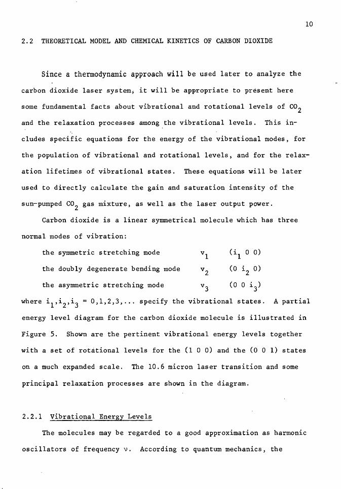
2.2 THEORETICAL MODEL AND CHEMICAL KINETICS OF CARBON DIOXIDE
Since a thermodynamic approach will be used later to analyze the
carbon dioxide laser system; it will be appropriate to present here
some fundamental facts about vibrational and rotational levels of co2
and the relaxation processes among the vibrational levels. This in
cludes specific equations for the energy of the vibrational modes, for
the population of vibrational and rotational levels, and for the relax
ation lifetimes of vibrational states. These equations will be later
used to directly calculate the gain and saturation intensity of the
sun-pumped co2
gas mixture, as well as the laser output power.
Carbon dioxide is a linear symmetrical molecule which has three
normal modes of vibration:
the symmetric stretching mode
the doubly degenerate bending mode
the asymmetric stretching mode
(il 0 0)
(0 i2 0)
(0 0 i3)
where i1,i
2,i
3 = 0,1,2,3, ... specify the vibrational states. A partial
energy level diagram for the carbon dioxide molecule is illustrated in
Figure 5. Shown are the pertinent vibrational energy levels together
with a set of rotational levels for the (1 0 0) and the (0 0 1) states
on a much expanded scale. The 10.6 micron laser transition and some
principal relaxation processes are shown in the diagram.
2.2.l Vibrational Energy Levels
The molecules may be regarded to a good approximation as harmonic
oscillators of frequency v. According to quantum mechanics, the
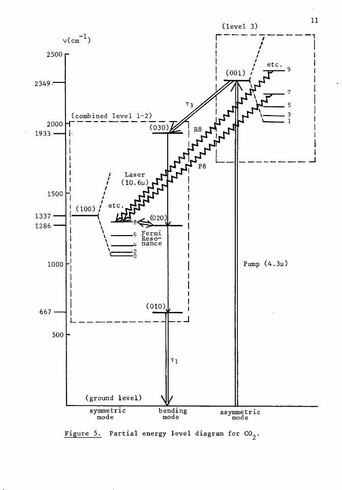
-1 · v (cm )
2500
2349-
2000 1933
1500
1337 1286
1000
667
500
(combined level 1-2)
I·. I I I I I I
I
I I I
I I
I I
<loo) I ( \ \ \ ---6 Fermi \ Reso\
\ ---+ nance '·---2 ---o
(010)
L----------- _ _J
(ground level)
symmetric mode
bending mode
---3 ---1
Pump (4.3µ)
asymmetric mode
Figure 5. Partial energy level diagram for co2
.
11
degrees of vibrational excitation are quantized and the permissible
energy states of a molecule are given by
e:. = (i + 32)h\) l.
where i = 0,1,2,3, (2)
Omitting the zero-point energy s = ~hv of a vibrational ground state 0
(i.e. vibrational energies are measured from the ground state),
s. = ihv l.
where i = 0,1,2,3, ...
Now th~· vibrational partition function is introduced (i.e. how
(3)
the particles are partitioned or divided up among the energy states),
as defined by
00
Q = E exp(-s./kT ) v i=O i v
00
L: i=O
exp(-ihv/kT ) v
where T is the vibrational temperature. That temperature is, in v
effect, defined in the Einstein function of equation (7) below.
When T = T (gas temperature), a thermodymanic non-equilibrium conv
(4)
dition exists. Note that T (and E shown later) indicates the degree v v
12
of population of a certain vibrational state; the higher the vibration-
al temperature, the larger the population of the vibrational state.
The sum in equation (4) is recognized as the geometrical series
where
= l/[1-exp(-e /T )] v v
e = hv/k v
characteristic temperature for vibration
Using equation (5) and the relation18
E v
(5)
(6)
where N is the total population density of co2
, the total vibrational
energy of the o~cillators per unit volume is
E = Nke I [exp ( e /T ) - iJ v v v v (7)
This is the well known Einstein function (in terms of vibrational
temperature T ) for a simple harmonic oscillator with a Boltzmann v
distribution of the states.
When T is in equilibrium with the translational temperature T v
(i.e. T = T), v
E = Nk8 /[exp(e /T) - l] v v v
The population distribution for the i-th vibrational level is
18 given by the formula
where
N./N = exp(-ie /T )/Q i v v v
N.: population density of the i-th vibrational level i
N : total population density
Now, from the ideal gas law
13
(8)
(9)
N(molecules/cm3) = 7.37 x 10² p (atm)/T(°K) (10) c
So far we have been referring to one vibrational mode. However,
since carbon dioxide has three modes, the vibrational partition function
Qv for co2 is (taking the double degeneracy of the bending mode into
account)
2 Qv = Ql Q2 QJ (11)
= { [1 - exp(-e 1 /T 1~ [1 - exp(-8/T2
)] 2 [1 - exp(-e 3/T3)] }-l (12)
where Q1
, Q2
, and Q3
correspond to the v1
, v 2 , and v3 modes, respectively.
Then, the energies of the three modes are, respectively,
2 Nke 1; [exp(e 1
/T1 )-1] ( 13) El = NkTl (cH,nQV/aTl) = for v1
mode
E2 = NkT~(3£nQV/aT2) = 2Nk8 2
; [exp(e 2
/T2)-l] for v
2 mode (14)
E3 = NkT2 (a~nQ /8T3) = Nk8 3
/ [exp( 8 3
/T3 )-1] for v3
mode (15) 3 v
14
where T1
,T2
, and T3
are the vibrational temperatures of the v1
,v2
, and
v3
modes, respectively, and e1,e
2, and e
3 are the characteristic
temperatures of vibration of the v1
,v2
, and v3
modes, respectively.
2.2.2 Rotational Energy Levels
Each vibrational level is subdivided into a number of rotational
levels denoted by J's. J can only be odd or even numbers for a given
vibrational level, and the selection rule for rotational transitions
is J = ± 1 (J = +l is a P-transition; J= -1 is an R-transition).
The quantized rotational energy is given by
EJ = hcBJ(J+l)
where
J = 0,1,2,3, .
B = rotational constant for each vibrational state
Taking the degeneracy gJ (=2J+l) into account, the rotational
partition function is
QR =Jio gJ exp(-c:J/kTR) J=even or odd
= ~ (2J+l) exp [-J(J+l)hcB/kTR] J=O .
J=even or odd
By approximating the series by an integral for a linear and
synnnetric molecule like co2
,
00
dJ (2J+l) QR = ~ f 0
exp [-J(J+l)hcB/kTR]
which can be shown to be 18
(16)
(17)
(18)
(19)
(20)
where
eR = hcB/k: characteristic temperature for rotation
TR = rotational temperature
Among the various rotational levels of a vibrational level a
15
Boltzmann distribution in terms of the gas temperature T(=TR) is es
tablished, which results from the fact that the spacing of the rotation-
al energy levels is compara~le to the kinetic energy (0.025eV) of a
molecule and these energies are easily exchanged in collisions
(thermalization).
Hence, at gas temperature T (=TR) the population of the J-th
rotational level is determined by 18
where
nJ population density of the J-th vibrational
rotational level
(21)
By differentiating this equation with respect to J, the value of
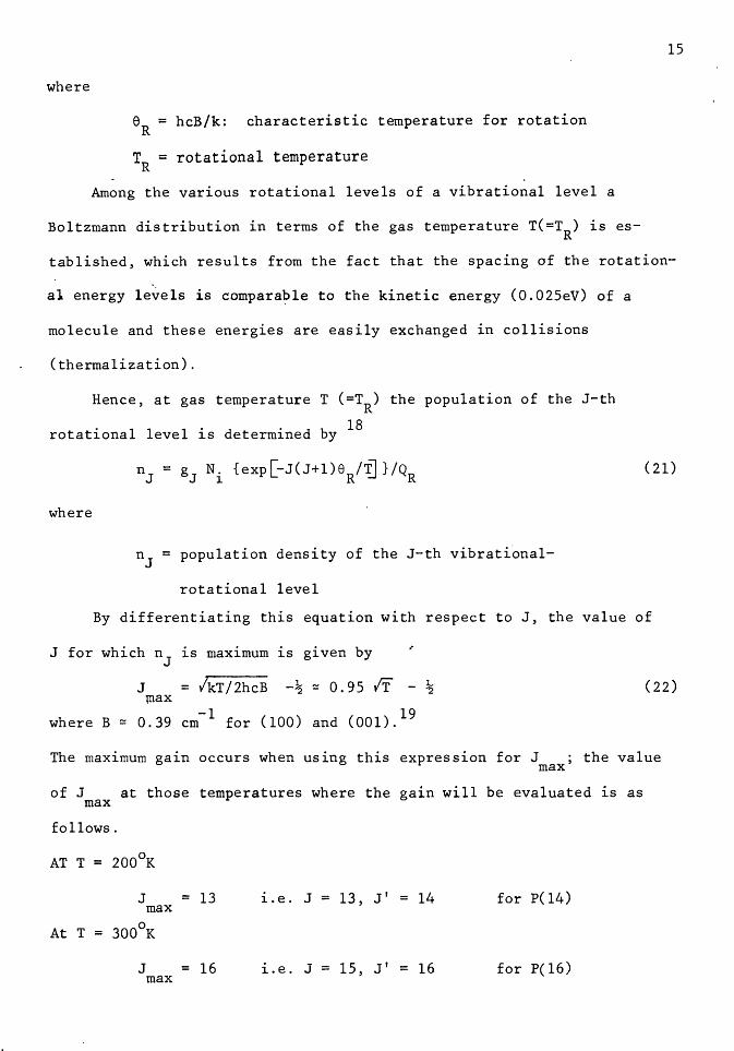
J for which nJ is maximum is given by ..
J = /kT/2hcB -~ :::: o.9s rr - ~ (22) ~ax
where B ~ 0.39 -1
for (100) and ( 001). 19 cm
The maximum gain occurs when using this expression for J ; the value max
of J at those temperatures where the gain will be evaluated is as max
follows.
AT T = 200°K
J = 13 max
At T = 300°K
J = 16 max
i.e. J = 13, J' = 14 for P(l4)
i.e. J = 15, J' = 16 for P( 16)
2.2.3 Vibrational Relaxation
Excited molecules in vibrational levels will decay in three
different fashions: by radiative decay (spontaneous emmission), col-
lisional deactivation and spatial diffusion. Over the pressure range
of interest in this study, the latter two processes are dominant since
the radiative decay lifetimes are considerably larger than the corr-
* spending collision or diffusion lifetimes.
One means of effectively raising the relaxation rate at which
molecules start or cease to interact with the lasing field is by
16
diffusions of molecules into and out of the laser beam (i.e. the region
in the gas where amplification exists). Diffusion can play an important
role in laser beams with both small radii and low total pressure.
expression for the diffusion lifetime Td is found to be 21-
23
l 8D T(°K)
p(torr) r 2 (cm) [1+4.Q,n(r/r )] 300
An
(23) T d (sec)
For a co2
-He mixture m. 23 m
where D = 400 cm torr/sec , the expression becomes
71 p(atm) r;(cm) [1 + 4 .Q,n(r/rm)] ..
T(°K)
where
D diffusion constant
r beam radius m
r radius of the tube
*The radiative lifetime Trad is about 2.5 msec for the (001) (100) transition (all P-transitions and R transitions), while for other transitions it is much larger.20
(24)
17
The second important deactivation process is collisional relaxation.
Since this is the dominant process for the pressure range of interest
in this study (i.e. p = 0.01-0.05 atm), the rest of our discussion will
be concerned with the detailed mechanism of collisional relaxation.
Transfer of energy between two vibrational states or one vibration-
al and one translational degree of freedom occurs through molecular
collisions. The collisional relaxation lifetime T (which is the average
time for a molecule to exist in an excited state before deactivation)
is defined by
where
T = T Z c
T : c
the time interval between collisions, which is
inversely proportional to pressure
Z the average number of collisions to deactivate one
vibrational quantum to its e-l value (i.e. l/Z is
the probability of deactivation of vibrational
energy in one collision)
(25)
In a mixture involving co2 and the foreign gas He (as noted later,
this mixture is chos:en for our laser system), relaxation of a vibration-
ally excited co2 molecule can take place through binary collision
processes with either ground state C02
molecule or with a He atom.
Th 1 . f b. 11' . . . by 24' 25 e re axation rate or inary co isions is given
where
1 PT
= "'c PTc-c
+ PTc-H
relaxation lifetime for collisions with co2
(26)
LC-H: relaxation lifetime for collisions with He
l/pTC-C: relaxation rate for pure C02 at p atm pressure
l/~LC-H: relaxation rate for collisions with He at p atm
pressure
¢C and WR: mole fractions of co2 and He, respectively
(¢ + ¢ = 1) C H
18
In what follows the kinetic reactions and the values of the life-
times TC-C and TC-H for the pertinent levels will be examined. In mod
eling the important kinetic processes involved in a co2 laser, certain
simplifications have been made as shown in the diagram of Figure 5. It
has been assumed that V - V (vibrational - vibrational) transitions are
very fast in each mode (i.e. in the vertical direction, such as (030) +
(020), (020) + (010), but not from one mode to any other (i.e. in the
horizontal direction). It should, however, be noted that process
(100) * 'co20) is very rapid because of the known Fermi resonance (F.R.).
Therefore, with this simplified model, mode v1 and v2
are considered to
be one combined level 1-2. Then, the rate-controlling processes.among
the groups of vibrational levels (i.e. level 3, comb~ned level 1-2, and
the ground level) are those from (001) to level 1-2 (i.e. lifetime T3
)
and from level (010) to ground level (i.e. lifetime T1
).
The pertinent processes for energy transfer between the noted
vibrational states can be expressed as kinetic reactions as follows:
T - V (translational - vibrational) processes:
T co
2 (010) + co
2 l,c-c :> -1
cm (27a) co2
+ co2
+ 667
19 T
co2
(010) + He l,C-H> co2
+ He + 667 -1 cm (27b)
v - V (vibrational - vibrational) processes: T
co2
(001) + co2
3 ,c-c> co2 (03~) + co2 + 416 -1 (27c) cm
T -1 co2
(001) + He 3,C-H;)ii. CO (030) + He + 416 cm (27d) 2
Crucial to laser oscillation is the fact that the lifetime of the
upper level T3
must be larger than the lifetime of the lower level T1
.
Only then can a population inversion be achieved. Furthermore, the
population inversion could be increased by enhancing the lower level
depopulation rate with the addition of helium.
*
*
The values of the collisional relaxation lifetimes T3 ,C-C' T3 ,C-H
Tl,C-C and Tl,C-H for the kinetic processes noted above have previously
been measured experimentally and are plotted versus temperature for
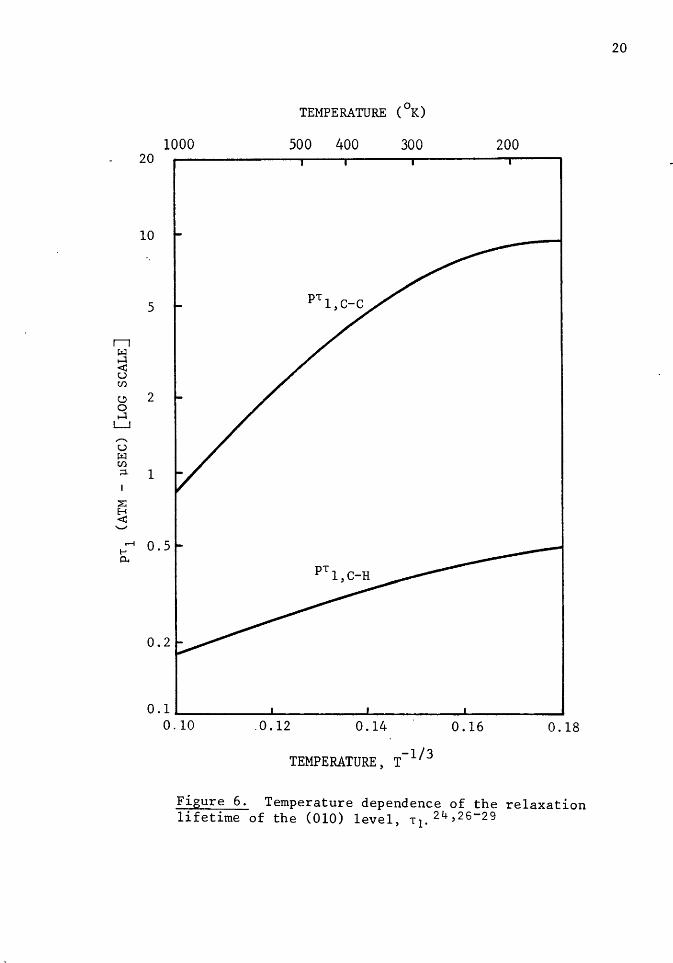
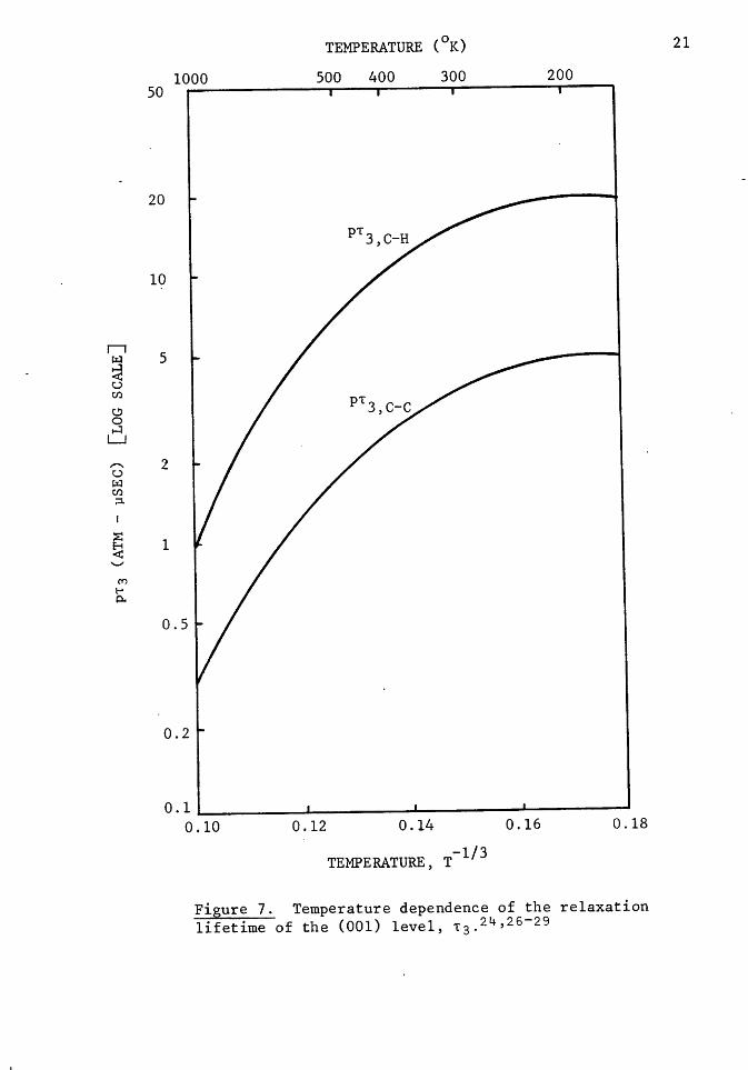
convenience in Figures 6 and 7. 24
' 26- 29 The lifetimes vary inversely
with pressure.
Now, since the diffusion effect on the upper level is considerable
and radiative decay ]. s not negligible in the lowest pressure range of
this study, a combined lifetime T3
which incroporates all
effects must be used; it l.S given as:
1 1 +
1 1 = +
T3 Td 3 T coll, 3 T rad,3 '
Note that the T3
referred to earlier was really Tcoll, 3 .
of Td 3 are calculated using equation (24). '
of these
(28)
The values
* Reactions (27c) and (27d) are considered to be dominant for the relaxation process from (001) to the 1-2 level. However, since those from (001) to any other levels in the 1-2 level could be responsible, T3,C-C and T3;C-H should be understood to correspond to the process from (001) to the whole 1-2 level.
11 µ::i ~ < u U)
c.!> 0 ~
L_J
,....... u µ::i U) ;:l.
~
~ .._,,
..-1 I-' 0..
TEMPERATURE (°K)
1000 500 400 300 200 20
10
5
2
1
0.5
0.2
O.lL-~~~~...L...~~~~-'-~~~~--i~~~~---0. 10 .0.12 0.14 0.16 0.18
TEMPERATURE T-l/3 '
Figure 6. Temperature dependence of the relaxation lifetime of the (010) level, T 1. 24,26-29
20
11 ~
~ C,.) Cl)
<::!> 0 ...:I LJ
-C,.)
~ Cl) ;:L
::E! ~ .._
Cf)
l-' p..
TEMPERATURE (°K)
500 400 300 200 50
20
10
5
2
1
0.5
0.2
0.1 L-----~----L~~----~"-~-------'-----------' 0.10 0.12 0.14 0.16 0.18
TEMPERATURE, T-l/3
Figure 7. Temperature dependence of the relaxation lifetime of the (001) level, T 3 .24,26-29
21
22
Therefore, combining the quations (24) and (26)
1 T (°K )
71 (atm) 2 (cm) [l + 4 in (r/rm)] T3 p r m
+[ iJJc 1/JH J p (atm)
1 ( 29) + + PT3 'c-c pT3,C-H 2.5 x 10⁻³
where
PT3 c-c = 3.76 atm µsec at 300°K . '
PT3 C-H = 15.5 atm µsec at 300°K '
The values of pT 3 ,C-C and PT3 C-H for 200°K are 1. 2 times those '
of 300°K.
Thus, in summary the pertinent mode energies, level populations,
and relaxation rates are functionally available to predict the actual
laser gain and the power output for a given set of conditions. The
necessary gain and output power relations which require the expressions
presented in this section are discussed in the following section.
2.3 PREDICTION OF GAIN AND POWER OUTPUT
2.3.1 Minimum Pumping Power Required for Population Inversion
When an electromagnetic field is applied to atoms (or molecules),
the interaction between the field and the atoms results in absorption
or stimulated emission depending upon the relative population in the
upper and lower levels. For any collection of atoms in thermal equi-
librium, there are always more atoms in a lower energy level than in a
higher energy level, and the transition is absorptive.
23
The essential feature of laser action is that under proper c1rcum-
stances, by pumping or exciting the atoms in appropriate fashion, a non-
equilibrium condition can be crec?-ted which produces a temporary "popu-
lation inversion" such that Boltzmann's law in terms of gas temperature
does not apply. In order to achieve a population inversion the availa-
b"le total pumping power, PT' must be greater than some minimum pumping
p h p . by 7 power, min' w ere min is given
where
Thus,
where
N1 Vhv p . = p min -r 3
\) = p
R >
R
c(A = c/4.3µ = pumping frequency p
Nihv E
T3
P /V = pumping power density T .
(30)
(31)
In terms of vibrational temperatures, the following relation has
to be satisfied for population inversion of the vibrational levels,
& = N. e -83 /T1 /Qy
N 1 N e -81 IT 1 / Q v
> 1 (32)
so that
T3 > ~ = 1.76 (33) Ti 81
Relations (31) and (33) will be useful to roughly check the possibility
of achieving lasing action.
2.3.2 Gain Coefficient
Electromagnetic radiation of intensity I propagating through an
24
amplifying medium (where a population inversion exists) with a gain
coefficient y will be amplified with an increase per unit length
dl = yl dz·
Or integrating
I(z) = I 0
yz e
That is, the intensity grows exponentially.
(34)
(35)
From the principle of energy conservation, the increase in intensi-
ty per unit length, dl/dz, is equal to the net power generated per unit
volume of length dz, i,e,
yl = g3 (n3 - ~)Whv g3 gl
where W, the induced emission rate, is given by
2· ) W = A_ I.g(v. = crI 8TI hv t hv
with sp
CJ optical cross section
g(v) line shape
(36)
(37)
g3, g1 : degeneracy of rotational levels of upper·and lower
vibrational levels, ~espectively
g3 = 2J + 1, gl = 2J' + 1
J' = J + 1 for P-transitions (strongest gain)
n 3 , n1: vibrational-rotational populations of upper and lower
-3 levels, respectively (cm )
Therefore, the expression of gain is obtained as
y =
where
8 1T t. sp
(38)
t spontaneous emission lifetime (t for the P-laser tran-sp sp
sition at 10.6µ is 5.38 sec)30
25
g(v) lineshape function which describes the distribution
of emitted intensity versus the frequency v; it is +oo
normalized according to f g(v)dv = 1 -oo
For the pressure broadening case (which applies to most of the
pressure range in this study), b.vL
g( v ) = ----------0 2n [( v-v o) 2+( b.vL/ 2 )2 J
= 2 (since v=v)
0 (39)
where b.vL is the Lorentzian linewidth which is given by the equation
A 1 --~ uVL = 1T Tc 1T
The collision frequency Ve for C02
is in general given by
where
cr c-k
c c-k
v = l: N cr c c k k c-k c-k
the population of each species
the collision cross section of each species with co2 the mean relative velocity of the species
= /8kr cc-k I~'
1 m
= 1 m
c
1 + -~
the mass of a molecule of each species
me the mass of a co2 molecule
In the case of a co2
-He mixture
v c
. (40)
(41)
(42)
While the above can in general be used to calculate b.vL' experimental
values of crC-H are required. Recent experiments have resulted in the
f 11 . f 1 . 31 o owing ormu ation
(43)
The results obtained by using equati-on (43) are in good accord with
the results obtained by using the more general equations noted above.
·For the combined Doppler and pressure broadening case (Voigt
Profile), 32 , 33 which applies to the lowest pressure range of this
study,
where
g( \) ) 0
2 exp ( x ) erfc(x)
l::.vD : Doppler Linewidth
x = /in.2 !::.vL/!::.vD
. 6 = (3.05 x 10 ) frfHz for a co2 line
erfc(x) : complimentary error function, whose values are
tabulated or given by 2 oo -u2
erfc(x) = f du e ;-; x
It is easily verified that the lineshape function reduces to the
results for pure Doppler or pressure broadening, if the limit x -+
0 or x-+ 00 is taken in equation (44):
1) Doppler broadened limit: x-+ 0
g(v ) -+ 2/in2 0 v'TI!::.v
2) Pressure broadened limit: x -+ 00
g(vo) -+ 2
TI tivL
(44)
(45)
(46)
(47)
(48)
(49)
2 -where the asymptotic relation exp (x ) ~ erfc (x) 41/(x/n ) was used.
Now recalling the relations for rotational and vibrational
populations, as given by equations (21) and (9), the rotational and
vibrational populations of the upper and lower levels are given by
~ e -J(J+l)8R/T
= (50) g3N3 QR
El__ -J ' < J ' + 1 ) e RI T
= e (51) g1N1 QR
26
27 -83/T3
N3 N e ~ E3
= = (52) Qv Qv k83
N -81/T1 _h_ E12
Nl = e = ~ ( 53)
Qv Qv
where
N total co2
population
N3
,N1
: population densities of the upper and lower vibrational
levels, respectively
population densities of the upper and lower rotational-
vibrational levels, respectively
vibrational temperatures of the upper and lower levels,
respectively
and where
E = Nke 3 I [ e 8 3 /T 3 - 1 J (15) 3
El2 = El+E2 = Nk8i/{ 1/ [eSi/T~-1] + 1/ [e62/TL1J} (54)
~3 = [ 1 - e-63/T3 J (SS)
~l = e-81/T1; [Ce81/Ti_1)-l + (e82/Ti_ 1)-l] (56)
Qv = [O-e-81/T1) ( l-e-62/T1)2 (l-e-83/T3)]-l (12)
T2
is assumed equal to T1
(by Fermi resonance).
Hence, the gain can be expressed in terms of the energies of the modes
where (Go) =
N
-J(J+l)6 R /T e
(57)
(58)
(59)
(60)
( 61)
28
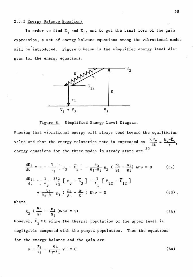
2.3.3 Energy Balance Equations
In order to find E3
and E12
and to get the final form of the gain
expression, a set of energy balance equations among the vibrational modes
will be introduced. Figure 8 below is the simplified energy level dia-
gram for the energy equations.
·.
R
Figure 8. Simplified Energy Level Diagram.
Knowing that vibrational energy will always tend toward the equilibrium
value and that the energy relaxation rate is expressed as dEv = Ev-Ev dt- T
energy equations for the three modes in steady state are 30
dE3 R - 1 [ E3 - E3 J 83 ( E.l £1.) Wh\J 0 = - g3 = dt T3 63-81 g3 ·g1 (62)
E!l.2. 1 382 [ E3 "E3] - ./1 [ El2 - El2 J =
~ dt . T3
+ el g3 ( .!!3_ - .!!l ) Wh\J = 0
83-61 g3 g1 (63) .
where
( ~3 _ n, ) g
3 ~ Whv = yl
g3 81 (34)
However, E3
~ 0 since the thermal population of the upper level is
negligible compared with the pumped population. Then the equations
for the energy balance and the gain are
R - !3. -~ yl = 0 T3 6 3-8 1
(64)
_l_~E 1 [ E12 - E12 J e,
+ YI T 3 83 3 Tl 83-81
G- 1 [ ~ t,;1E J Y= {__£) N kQ 8 3 E3 - 81 12
v Thus, there are the three unknowns E
3, E12' y
above; solving for Y,
29
= 0 (65)
(60)
in the three equations
For a small signal (where I =::Q) in the energy equations, (64), (65),
and ( 60)
Therefore
Also,
where
therefore
where
The small
e .Q.n(NkG.3.. + l)
T3R
= kN81 ~l
signal gain Y0 is · Go 1
Yo = <N) kQ v
(Go) 1 = N kQ
v
(67)
(68)
( 69)
(70)
(71)
(72)
(60)
(73)
30
Thus, for a small signal (I~ 0), the values of the vibrational tempera-
tures T3 , T1 and the gain (~mall signal gain) Y0
can be calculated from
equations (68), (71), and (73).
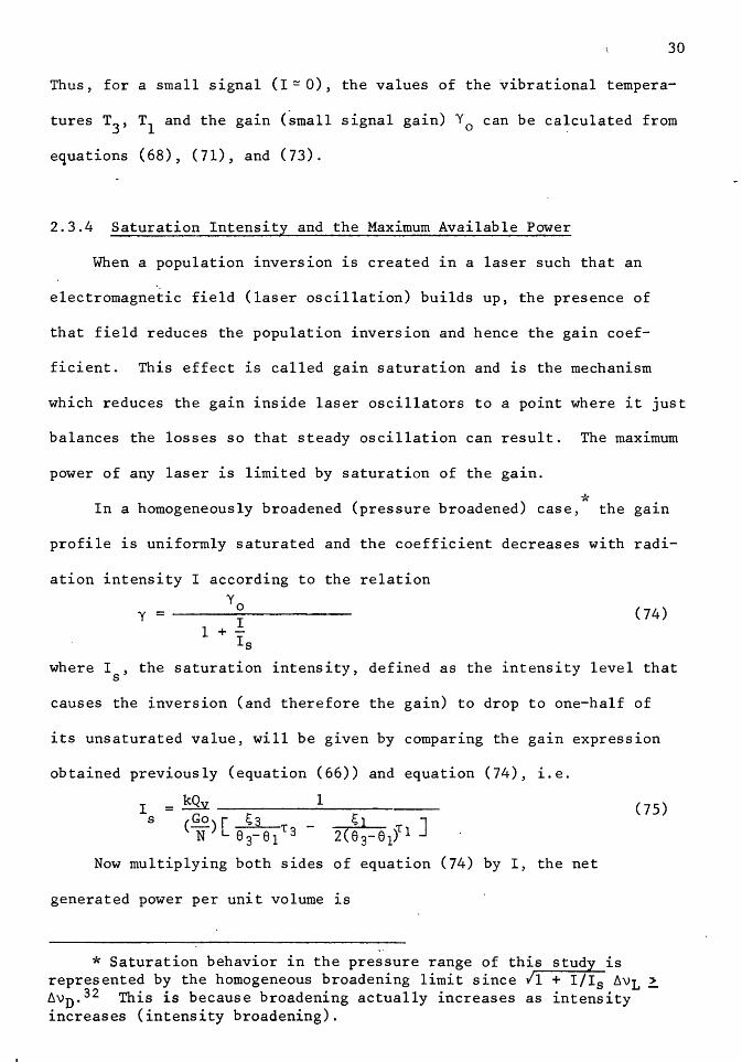
2.3.4 Saturation Intensity and the Maximum Available Power
When a population inversion is created in a laser such that an
electromagnetic field (laser oscillation) builds up, the presence of
that field reduces the population inversion and hence the gain coef-
ficient. This effect is called gain saturation and is the mechanism
which reduces the gain inside laser oscillators to a point where it just
balances the losses so that steady oscillation can result. The maximum
power of any laser is limited by saturation of the gain.
* In a homogeneously broadened (pressure broadened) case, the gain
profile is uniformly saturated and the coefficient decreases with radi-
ation intensity I according yo
to the relation
y = ~~~~I~~~~~~-1 + -
Is
(74)
where I , the saturation intensity, defined as the intensity level that s
causes the inversion (and therefore the gain) to drop to one-half of
its unsaturated value, will be given by comparing the gain expression
obtained previously (equation (66)) and equation (74), i.e.
I s
Now multiplying both sides of equation (74) by I, the net
generated power per unit volume is
(75)
* Saturation behavior in the pressure range of this study is represented by the homogeneous broadening limit since 11 + I/Is 6v1 ~ 6vn. 32 This is because broadening actually increases as intensity increases (intensity broadening).
IY ·o IY = ----
1 + I ·r s
= I y ( 1 s 0
I s
I + I ) s
and its profile is plotted in Figure 9 below.
:>H
Figure 9.
-- - -- -- - - - - - - -- -:....=-:...-==-----------
I s
INTENSI~, I
Net generated power per unit volume versus intensity.
31
(74)
As can be seen from Figure 9, the maximum available power per unit
volume is I Y (where I>> I), the value of which is given by the ex-s 0 s
pression below as obtained from equations (73) and (75).
p max
v m
I y s 0
2.3.5 Cavity Losses and Output Coupling
( 77)
So far we have not considered cavity losses such as those due to
scattering, absorption, diffraction (these are called residual losses),
and useful output transmission. But in order to figure the actual
output power, we have to det~rmine those losses.
Scattering and absorption by the mirrors will generally be small
and is usually less than a percent (mainly by absorption). Diffraction
is dependent on many parameters such as cavity length ~' radius of the
mirrors, curvature of the mirrors, and the transverse mode configuration
of the laser beam. For the cavity dimensions found necessary in this
study t~e diffraction loss can be held to less than a percent (see
Section 3 . 1. 1 ) .
Regarding the output loss, it should be noted that there is a
trade-off between the two extremes; i.e. if output mirror loss is too
32
large, internal cavity losses are too large for laser oscillation, and
on the other hand if the mirror transmission is too small, almost no
useful power is coupled out.
The fraction of the intensity lost per single pass, L, is
where
L = L. + T i
(78)
L.: i
T :
residual loss per single pass
useful mirror transmission (average of both mirrors)
Th . T th t t .:s . by34
e optimum to maximize e power ou pu ~ given
(79) T = -L. + /y 0 .Q.L. opt i i
2.3.6 Threshold Gain and Output Power
Once the oscillation starts, the gain is reduced by gain satu-
ration and clamped at the threshold value regardless of the pumping.
At this point the gain per pass is equal to the loss per pass, i.e.
y t.Q. = L (80)
This is valid for small losses, i.e. L <<l.
From equation (80) and (74) at threshold, the intensity I can be written
as
I = I s
(81)
33
The cavity power considering losses is consequently given by
P = (IY )V = I A (Y t - L) · e t m sm 0 (82)
where A = V /i is the cross-sectional area of the beam. m m
The fraction of the cavity power that is coupled out of the laser
cavity as a useful output is T/L.
The power output is thus,
p 0
T = - p L e
(83)
Combining equations (73), (75), (82), and (83), P is finally writte.n 0
as
p 0
(84)
34
3. RESULTS AND DISCUSSION
A eomputer program was written to facilitate the calculation of
small signal gain Yo, maximum available power P , cavity power P , max e
output power P , optimum mirror transmission T , efficiency o opt
(n=P0 /PT) and vibrational temperatures T3 and T1 of the upper and lower
levels for any set of parameters for the co2-He laser system. A
co2-He mixture was chosen as the laser medium; addition of helium
effectively depopulates the lower level while populating the upper level
only by a slight degree. Nitrogen was not used because it provides no
advantage to a sun-pumped co2
laser. The parameters that were varied
included the gas temperature T, the total gas pressure p, the' partial
pressure of carbon dioxide p , the beam radius r , the radius of the c m
tube r, the length of the tube ~' the absorption path length of the
sunlight~ , the residual loss per pass 1., and the area of the solar a i
energy collector A . Total pressure was varied in the range of s
p = 0.01 - 0.05 atm where acceptable gain and output power were found
to exist. 0 0 '
Gas temperatures of 200 K and 300 K were taken since at
lower temperatures (about 170°K) carbon dioxide solidifies, and at
temperatures above 300°K the gain was found to be too low for laser
oscillation because of thermal population of the lower level.
Computed results are given first for a specific system model and
then the effects on the laser performance of varying selected parameters
are examined. The proposed system model is described in the following
section.
35
3.1 PROPOSED LASER SYSTEM MODEL
Description of the System 3.1.1
End pumping was chosen because it provides the necessary long sun-
light absorption path length in comparison to side pumping. Side pumping
is of course possible as another alternative approach that could be
studied. Although the length of the tube should be long to allow enough
absorption, it cannot be too long because of practical size limitations
and a higher diffraction loss. A tube of 1 m length was arbitrarily
chosen with a 2 m absorption path length for the sunlight (i.e. one
round-trip of the incident sunlight in the tube is assumed).
A collector size of 10 m2
was also arbitrarily chosen as the la~gest
reasonable collector size physically and economically practical. The
2 minimum possible spot size concentrated from a 10 m collector is
limited to a 1.66 cm diameter area by the Abbe sine condition; therefore,
the radius of the tube was determined to be 0.85 mm.
The radius of the beam should be large so that as many of the
excited molecules as possible participate in lasing action. This is
especially important for a sun-pumped co2 laser since the pump light
is limited by collector size and should not be wasted. On the other hand,
beam size for a given tube radius is limited by diffraction; the diffrac-
2 tion loss for a single mode beam is 1% for rm= 3r·. and even larger
for a multl..mode beam. 36 Th b d' · h f k b e earn ra ius is t ere ore ta en to e
5 mm in the initial case.
36
The parameters for the laser tube and the collector area were
thus selected as follows:
Area of the sun collector, A s
= 10
Residual loss per pass, L. = 1 % 1.
Beam radius, r = 0.5 cm m
Radius ·of the tube, r = 0.85
Length of the tube, ~ = 1 m
cm
2 m
Absorption path length of the sunlight, i a
3.1. 2 Computed Results for Proposed Laser
= 2 m
Computed results for small signal gain and output power are pre-
sented here .:is a funcdon or the gas temperatUre arid the total and partial
pressures. The gain and power generally decrease as the gas temperature
goes up because of the increase of the lower level population which is
almost in equilibrium with the gas temperature. Thus, for the range of
gas temperatures considered, the lowest possible temperature is optimum
for this system.
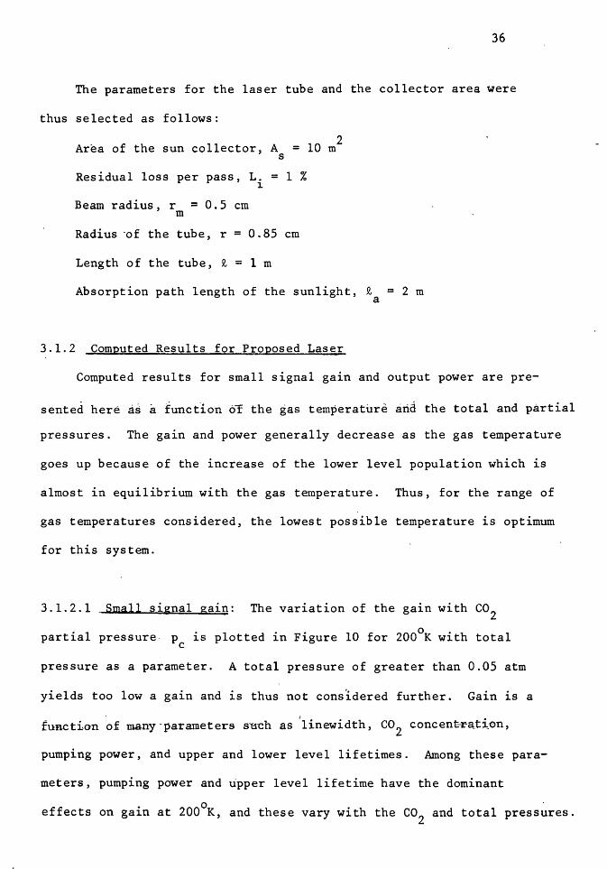
3.1.2.1 Small signal gain: The variation of the gain with co2
partial pressure- p is plotted in Figure 10 for 200°K with total c
pressure as a parameter. A total pressure of greater than 0.05 atm
yields too low a gain and is thus not consldered further. Gain is a • J
function of many-parameters su~h as linewidth, co2
concent-rat~~n,
pumping power, and upper and lower level lifetimes. Among these para-
meters, pumping power and upper level lifetime have the dominant
0 effects on gain at 200 K, and these vary with the co
2 and total pressures.
,,-... ~ ~ E-4 ~ ~
........... ~ '-"
z H < l!>
~ z l!> H Cl)
....:l
....:l
~ Cl)
37
8
p=0.01 ATM 6
4
2
o.__ __________ _._ __________ --' ____________ ...._ __________ __ 0 0.005 0.01 .015 0.02
co2 PRESSURE (ATM)
Figure 10. Variation of small signal gain with total and partial pressures.
I
I
38
As the co2 and total pressures increase, pumping power increases, but
the upper level lifetime decreases. The maximum gain, then, occurs
when the product of pumping power and upper level lifetime is a
maximum. Because pumping is relatively weak such that the effect of
the relaxation of the upper level predominates, maximum gain occurs at
low partial and total pressures. At these low pressures thermal
population of the lower level (100) is almost negligible cOmpared
with that of the pumped population of the upper level (001). Although
the maximum gain is given at p = 0.01 atm and pc= 0.005 atm, maximum
output power is achieved at higher pressures (with high enough gain)
as will be seen in the next section.
At 300°K thermalization of the lower level reduces the gain con-
siderably to a value which is generally too low to.be able to enable
lasing action. A maximum gain of only 2.5%/meter was obtained in the
300°K case. 0 Hence, the gas temperature was held at 200 K.
3.1.2.2 Output Power: Shown in Figure 11 is the plot of output power
at 200°K. Output power is the power which comes out of the laser cavity
through the partially transmitting mirror whose optimum transmission is
calculated from equation (79). As one can see from expressions (82)
and (83), output power varies with saturation intensity, small signal
gain and residual losses as well as beam volume. Saturation intensity
is a function of linewidth, pumping power, and upper and lower level
lifetimes.
,..... tll E-4
~ ~ H H H H :a: .......,
i::z:: r:i::I
5 P-t
E-4 :::> P-t E-4 :::> 0
250
200
150
100
50
0
= 0.01 ATM
= 0.05 ATM
.005 .01 .015
co2 PRESSURE (ATM)
Figure 11. Variation of output power with total and partial pressures.
39
.02
40
At 200°K a maximum output power of about 250 milliwatts was
obtained at p = 0.02 atm and p = 0.01 atm with 1.3% mirror transc
missionA These pressures correspond to a rather low, non-optimum
gain of 5.4%/meter, which would, however, still be sufficient to
sustain laser oscillation.
3.1.2.3 Oyerall Performance: Enough gain and high output power are
the requirements for good laser performance. Since the sun-pumped
co2 laser is found to be a modest power, low gain system, it must
operate at conditions where the gain is sufficient and the power is
highest. The optimum performance of the assumed laser system is
summarized as follows:
Temperature:
Total pressure: 0.02 atm
co2 pressure: 0.01 atm
Small signal gain: 5.4%/meter or 5.4%/pass
Output power: 250 milliwatts
Efficiency: 4.1%
Optimum mirror transmission: 1.3%
3~2 EFFECTS OF PARAMETER VARIATION ON THE SMALL SIGNAL GAIN
AND THE OUTPUT POWER
0 For the selected temperat~re of 200 K, various parameters that
were preselected to initially determine the gain and the output power
l I . 41
are now varied to note the sensitivity of the performance to varia-
tions of the individual variables.
Each of the Figures 12-15 shows the variation of the gain and the
output power due to the change of one parameter selected from the pro-
posed system model; the six parameters changed are residual loss L., i
collector area A , radii of the beam r and the tube r, and the lengths s m
of the absorption path t and the tube t. a
The effect of varying residual losses is noted in Figure 12.
The losses are taken to increase from 1% to 2% and then to 3%. The gain
remains the same since it is independent of losses, but the output
power decreases to 1/2 for L. = 2%, and to 1/3 for L. = 3%. i 1
Achieving
losses of less than 1% would be difficult, but would result in a large
power increase. Thus, the magnitude of residual loss is an important
parameter.
The collector size directly affects the output power and gain as
shown in Figure 13. As collector size varies, tube radius and beam
radius are also adjusted accordingly. The tube radius was matched with
the minimum spot size (by the Abbe Sine conditio.n) concentrated from
each collector area. The beam radius was kept slightly smaller than
2/3 of the tube radius for minimum diffraction loss. Since the pumping
power density stays the same with varying collector size and, hence,
tube radius (i.e. the maximum intensity of concentrated sunlight is
limited by ilie Abbe Sine condition), the gain stays essentially con-
stant. On the other hand, output power increases proportionally with
collector size and, hence, with beam volume. For example, by reducing
collector by one-half (from 10 m 2 2 area to 5 m ) so that the beam volume
,,-....
Cf)
E-1
~ :3 H H H H ~
..........
~ i:.:r.:l
5 ~
E-1 :::> ~ E-1 :::> 0
350
300
250
200
150
100
50
OL-------------L--~--------.J---~--~----'--------------i 0 1 2 3 4
Figure 12. at 200°K.
RESIDUAL LOSS PER PASS (%)
Output power versus residual loss per pass
42
-.. Cf.)
E-1
~ ~ H ...:I ...:I H ~ --~ ~
~ Pol
E-1 :::::> Pol E-1 :::::> 0
43
12
400 10
-.. 8 ~
~ E-1
300 ~ .......... ~ --z H
6 ~
~ G
200 H Cf.)
H
~ 4 ~
Cf.)
2
J
I
(or beam spot size) is decreased by one-half, the output power goes
down by one-half, while the pumping power density and, therefore, the
gain stays constant. Although power increases with collector area,
considering physical constraints, a collector much larger than 10 m2
would not be very practical. Besides, a larger beam size is also
required for a larger collector. That would also be hard to achieve.
For thi'constant collector (10 m2) and the tube size (0.85 cm
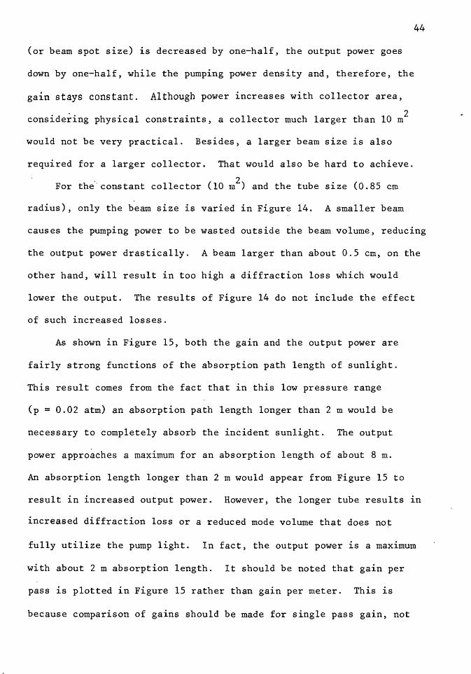
radius), only the beam size is varied in Figure 14. A smaller beam
44
causes the pumping power to be wasted outside the beam volume, reducing
the output power drastically. A beam larger than about 0.5 cm, on the
other hand, will result in too high a diffraction loss which would
lower the output. The results of Figure 14 do not include the effect
of such increased losses.
As shown in Figure 15, both the gain and the output power are
fairly strong functions of the absorption path length of sunlight.
This result comes from the fact that in this low pressure range
(p = 0.02 atm) an absorption path length longer than 2 m would be
necessary to completely absorb the incident sunlight. The output
power approaches a maximum for an absorption length of about 8 m.
An absorption length longer than 2 m would appear from Figure 15 to
result in increased output power. However, the longer tube results in
increased diffraction loss or a reduced mode volume that does not
fully utilize the pump light. In fact, the output power is a maximum
with about 2 m absorption length. It should be noted that gain per
pass is plotted in Figure 15 r~ther than gain per meter. This is
because comparison of gains should be made for single pass gain, not
_J
350
300
,,....... 250 Cf.)
E-1 E-1 < ~ H ...:I ...:I H ~
........ 200 ~
~ P-i
E-1 :=> P-1 E-1 :::> 150 0
100
50
1 2 3 4 5
BEAM RADIUS (MILLIMETER)
Figure 14. Output power and small signal gain versus beam radius:.
7
6
5
4
3
2
1
45
-~ ~ E-1
~ ........ N ........
z H < ~
...:I < z ~ H Cf.)
...:I
~ Cf.)
_J
I
I
,,...... CJ)
~
~ :;: H H ...:l H ~ '-'
A:::
~ 0 l1i
~ :::> l1i ~ :::> 0
409
350
300
250
200
150
100
50
o ____ ~-------~----~--~--~------'----------....... ----__, 0 2 4 6 8
ABSORPTION PATH LENGTH (METER)
Figure 15. Output power and small signal gain per pass versus absorption path length at 200°K.
46
28
24 ,,...... IN? '-'
CJ)
t/l < l1i
20 A::: w l1i
z H < C!>
16 ~ z C!> H CJ)
H
~ 12 t/l
8
4
_J
47
gain per unit length for different tube lengths.
In sunnnary, when the various parameters are varied as above, the
output power varies more than the gain. The initially proposed laser
system in fact has the optimum power and reasonable gain. However,
it is not likely that more than 500 milliwatts could be obtained from
the sun-pumped co2 laser design presented here.
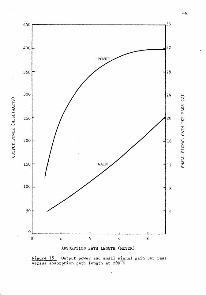
3.3 PRACTICAL DESIGN CONSIDERATIONS
In the foregoing discussions it has been assumed that the sun-
light could appropriately be collected, concentrated, an~ then absorbed
in the co2
gas mixtures. A schematic diagram of the end-pumping method
assumed is shown in Figure 16 below.
Sunlight
1.7 cm dia x 100 cm long laser tube
Output mirror
c::::::J===i Laser Output (10.6µ)
Wall of high internal reflectivity for sunlight (4.3µ)
Figure 16. Schematic diagram of a sun-pumped co2
laser with end-pumping.
m2 parabolic collector
48
In this scheme sunlight collected by a large parabolic collector is
focused into a lens that produces essentially parallel pump light
which is transmitted into the laser tube. Other possible means of
collecting and leading sunlight into the laser tube could be developed
and used. For example, side-pumping might be another alternative
method if long sunlight absorption path lengths could be achieved.
The laser output mirror and sunlight input mirror must be
appropriately coated so that they transmit light selectively according
to wavelength; the output mirror is partially transmitting for 10.6
micron laser light and reflective for 4.3 micron pumping light. The
input mirror is transparent in the 4.3 micron region and reflective
at 10.6 microns.
The other main practical consideration for a sun-pumped space-
qualified co2
laser is cooling the laser medium. Conductive cooling
of the laser tube and use of heat pipes to remove the heat to a
radiative cooler is considered to be the preferred design technique
for a space qualified laser because of its low weight and high
1 . b·1· 1,5 re 1a 1 ity.
4. CONCLUSIONS
The possibility of directly sun-pumping a CW co2
laser in space
has been analyzed for the first time, and the gas kinetic analysis
indicates that end-pumping such a laser is feasible. However, since
this laser system is pump deficient, it is essential to keep the
residual losses such as diffraction, absorption, and scattering to a
minimum, and also to concentrate the sunlight down to an almost
theoretical minimum spot size in order to obtain the highest pumping
power density. The gas temperature must also be held low (but
higher than about 170°K) to achieve the highest possible gain and
output power.
Since pumping must take place at low gas pressures to achieve
sufficient gain, the power output is modest. In principle the out
put can be increased by utilizing a larger sunlight collector area,
but practical difficulties with a larger collector and the necessarily
larger laser beam diameter limit this approach. Long absorption
paths could also be used to achieve higher powers, but the amount of
improvement is again practically limited. It is possible that
addition of other gases to the co2
-He mixture could increase the
output power by increasing the absorption of sunlight without ad
versely affecting the upper level lifetime. This possibility for
increasing the output should be further examined. Nonetheless, at
this time it would appear that the maximum achievable continuous
power obtainable with the laser design presented here is about 500
50
milliwatts. Therefore, it does not look like high powers can
be achieved using this approach. In addition, it should be noted
that this particular type of co2 laser would not appear to be capable
of operation at pressures above atmospheric where continuous tunability
can be achieved.
It should be noted that output powers of greater than one watt
have already' been achieved with a sun-pumped Nd:YAG laser. However,
if it is desirable or necessary to utilize a modest power carbon
dioxide laser or if its output wavelength is preferred, then this
study shows that such a laser is feasible. To examine its per-
formance in more detail, laboratory measurements would have to be
made to determine how much sunlight can actually be absorbed and
how much gain can be achieved under the conditions predicted to
give optimum performance.
REFERENCES
1. J.D. Foster and R.F. Kirk, "Space Qualified Nd:YAG Laser·," Final Technical Report, Contract No. NAS102-2160, June 1970.
2. C.G. Young, "A Sun Pumped CW One-Watt Laser," Applied Optics, Vol. 5, No. 6, p. 993, June 1966.
3. G.R. Simpson, "Continous Sun-Pumped Room Temperature Glass Laser Operation," Applied Optics, Vol. 3, No. 6, p. 783, June 1964.
4. D.F. Nelson and N.S. Boyle, "A Continuously Operating Ruby Optical Maser," Applied Optics, Vol. 1, No. 2, p. 181, March 1962.
5. L. Huff, "Sun Pumped Laser," Final Technical Report, Contract No. AFAL-TR-71-315, September 1971.
6. D.C. Forster, F.E. Goodwin, and W.B. Bridges, "Wide-Band Laser Communications in Space," IEEE Journal of Quantum Electronics, Vol. QE-8, No. 2, p. 263, February 1972.
7 · P.A. Bokhan and G. I. Talarkina, "On The Possibility of Optical Pumping of Gases by Their Own Radiation," Optics and Spectroscopy, Vol. 25, No. 4, p. 298, October 1968.
8. P.A. Bokhan, "On Optical Pumping of a Molecular Laser by Blackbody Radiation," Optics and Spectroscopy, Vol. 26, No. 5, p. 423, May 1969.
9. P.A. Bokhan, 1'Experimerit on Optical Pumping of a Carbon Dioxide Molecular Laser," Optics and Spectroscopy, Vol. 32, No. 4, p. 435, April 1972.
10. I. Wieder, "Flame Pumping and Infrared Maser Action in co
2, 11 Physics Letters, Vol. 24A, No. 13, p. 759, June 1967.
11. 0. Yesil and W.R. Christiansen, "Solar Pumped Continuous Wave Carbon Dioxide Laser," Progress in Astronautics and Aeronautics, Vol. 61, p. 357, January 1978.
12. H. Shirahata, S. Kawada and T. Sujioka, "Atmospheric Pressure CW co2 Laser Pumped by Blackbody Radiation," 5th Conference on Chemical and Molecular Lasers, St. Louis, Mo., April 1977.
51
13.
14.
15.
16.
17.
18.
REFERENCES (Cont'd)
T.Y. Chang and O.R. Wood, II, "Optically Pumped AtmosphericPressure co2 Laser," Applied Physics Letters, Vol. 21, No. 1, p. 19, July 1972.
T.Y. Chang and O.R. Wood, "Optically Pumped 33-atm CO Laser," Applied Physics Letters, Vol. 23, No. 7, p. 3~0, October 1973.
N. Robinson, Solar Radiation, Elsevier Publishing Company, New York, 1966, p. 2.
V . R. S t·u 11 , P . J . Wyatt , and G . N . P 1 as s , "The Infrared Transmittance of Carbon Dioxide," Applied Optics, Vol. 3, No. 2, p. 243, February 1964.
V.R. Stull, P.J. Wyatt, and G.N. Plass, "The Infrared Absorption of Carbon Dioxide, Infrared Transmission Studies," Vol. III, Report SSD-TDR-62-127, Space Systems Division, Air Force Systems Command, Los Angeles, California, January 1963.
W.G. Vincenti and C.H. Kruger, Jr., Introduction to Physical Gas Dynamics, John Wiley & Sons, Inc., New York, 1965, p. 133, p. i19, and p. 206.
19. V.P. Tychinskii, "Powerful Gas Lasers," Soviet Physics Uspekhi, Vol. 10, No. 2, p. 131, September 1967.
20. H. Statz, C.L. Tang, and G.F. Koster, "Transition Probabilities Between Laser States in Carbon Dioxide," Journal of Applied Physics, Vol. 37, No. 11, p. 4278, October 1966.
21. D.R. Whitehouse, "High Power Gas Laser Research," Final Technical Report, Contract DA01-021-AMC-12427(Z), p. 11, May 1967.
22. H. Granek, C. Freed, and H.A. Haus, "Experiment on Cross Relaxation in co2," IEEE Journal of Quantum Electronics, Vol. QE-8, No. 4, p. 404, April 1972.
23. H. Granek, "The Observation of Diffusion as an Effective Vibrational Relaxation Rate in CO ," IEEE Journal of Quantum Electronics, Vol. QE-10, ~o. 3, p. 320, March 1974.
24. J.T. Yardley and C.B. Moore, "Intramolecular Vibration-toVibration Energy Transfer in Carbon Dioxide," The Journal of Chemical Physics, Vol. 46, No. 11, p. 4491, June 1967.
25. A.K. Levine and A.J. DeMaria, Lasers, Marcel Dekker, Inc., New York, 1971, p. 150.
52
REFERENCES (Cont'd)
26. C.B. Moore, R.T. Wood, Bei-Lok Hu, and J.T. Yardley, "Vibrational Energy Transfer in co
2 Lasers," The Journal of
Chemical Physics, Vol. 46, No. 11, p. 4222, June 1967.
27. R.I:i. Taylor and S. Bitterman, "Survey of Vibrational Relaxation Data for Processes Important in the co2-N
2 Laser Systems,"
Reviews of Modern Physics, Vol. 41, No. 1, p. Z6, January 1969.
28. R.L. Taylor and S. Bitterman, "Survey of Vibrational Relaxation Data for Processes Important in the CO -N
2 Laser
System,h Research Report 282, Contract F33(615)-6~-C-1030, October 1967.
29. W.A. Rosser, Jr., A.D. Wood, and E.T. Gerry, "Deactivation of Vibrationally Excited Carbon Dioxide (~3) by Collisions with Carbon Dioxide or with Nitrogen," The Journal of Chemical Physics, Vol. 50, No. 11, p. 4996, June 1969.
30. A.L. Hoffman and G.C. Vlases, "A Simplified Model for Predicting Gain, Saturation, and Pulse Length for Gas Dynamic Lasers," IEEE Journal of Quantum Electronics, Vol. QE-8, No. 2, p. 46, February 1972.
31. R.L. Abrams, "Broadening Coefficients for the P(20) Laser Transition," Applied Physics Letters, Vol. 25, No. 10, p. 609, November 1974.
32. W.B. Lacina, "Kinetic Model and Theoretical Calculations For Steady State Analysis of Electrically Excited CO Laser Amplifier Systems," Final Report: Part II, Contract No. N00014-71-C-0037, p. 21, p. 35, August 1971.
33. D.J. Eckstrom, "Vibrational-Relaxation Measurements in Schock-:-Heated Carbon Dioxide by Tuned-Laser Absorptivity," SUIPR Report No. 414, SUDAAR No. 420, p. 106, Institute For Plasma Research, Stanford University, Stanford, California, March 1971.
34. A. Yariv, Introduction to Optical Electronics, Holt, ,Rinehart, and Winston, Inc., U.S.A., 1971, p. 111.
35. F.A. Jenkins and H.E. White, Fundamentals of Optics, McGrawHill Book Company, Inc., New York, 1957, p. 154.
36. A.E. Siegman, An Introduction to Lasers and Masers, McGrawHill Book Company, Inc., New York, 1971, p. 335.
53