Embed Size (px)
Citation preview
A FINITE DIFFERENCE SOLUTION TO THE TWO-DIMENSIONAL
WALL JET ON A COMBUSTION TURBINE BLADF
by
Martin David Harsh III
Thesis submitted to the Graduate Faculty of the
Virginia Polytechnic Institute and State University
in partial fulfillment of the requirements for the degree of
APPROVED:
Walter F! O'Brien
MASTER OF SCIENCE
in
Mechanical Engineering
Hal L. Moses, Chairman
May 1978
Blacksburg, Virginia
William C. Thomas
Acknowledgments
The author would like to express his gratitude to fellow
graduate students and faculty members in the College of Engineering
with whom he had the honor to associate while studying at Virginia
Polytechnic Institute and State University.
The author is indebted to of the Mechanical
Engineering Department for the opportunities and experience gained
as a teaching assistant.
A special thanks is extended to his parents,
and sisters,
Their support and encouragement is invaluable.
ii
Table of Contents
Acknowledgments •
Table of Contents • •
List of Figures •
List of Tables
Nomenclature
1. Introduction
2. Turbine Blade Geometry
3. Boundary Layer Analysis
4.
3.1 The Governing Equations
3.2 Finite Difference Form of the Boundary Layer Equations
3.3 Boundary Conditions
3.4 The Coordinate Transformation
3.5 The Eddy Viscosity Model .••
3.6 Boundary Layer Characteristics
3.7 The Algorithm for Solution to the Governing Equations . . • . .
3.8 The Wall-Jet Model . . Results . . . . . 4.1 Laminar Boundary Layer Calculations
4.2 Turbulent Boundary Layer Calculations
4.3 Wall-Jet Calculations . . . .
.
5. Conclusions and Recommendations for Further Study
lii
. ii
. iii
. • • • v
• • . vii
• viii
. 1
. 6
. . . 15
. 15
. 18
• 26
. 32
• 34
. 37
•. 39
. . . . . • 40
. 43
. .43
• 54
. . 65
. . 74
Table of Contents (continued)
Bibliography •
Appendix - The Crank-Nicolson Computer Code
Vi ta . . • • . . . . . . • · . •
Abstract
iv
• • • • 76
78
82
Figure No.
1
2
3
4
5
6
7
8
9
10
11
12
13
14
15
16
List of Figures
Title
Combustion Turbine Thermal Efficiency .
General Cambered Airfoil Section
C4, T6, and NACA 0012 Cambered Airfoil Sections with a 1 = 0°, a 2 = 60° . • • •
Comparison of Cambered NACA 0012 Airfoil Section with Large Industrial Combustion Turbine Vane . . . . . . . Boundary Layer Grid System
Solution to the Momentum Equation . Solution to the Equation Governing Conservation of Mass
Wall-Jet Model
u-Profile for Laminar Boundary-Layer Flow on a Flat Plate . . . . . . . . . v-Profile for Laminar Boundary-Layer Flow on a Flat Plate . . . . . . . . u-Profile for Laminar Boundary-Layer Flow on a 27° Half-Angle Wedge . u-Profile for Laminar Boundary-Layer Flow on a 16.2° Expansion Corner
Momentum Thickness for Various Laminar Boundary-Layer Flows . . . . . Skin Friction Coefficient for Various Laminar Boundary-Layer Flows . . . .
.
.
.
.
.
.
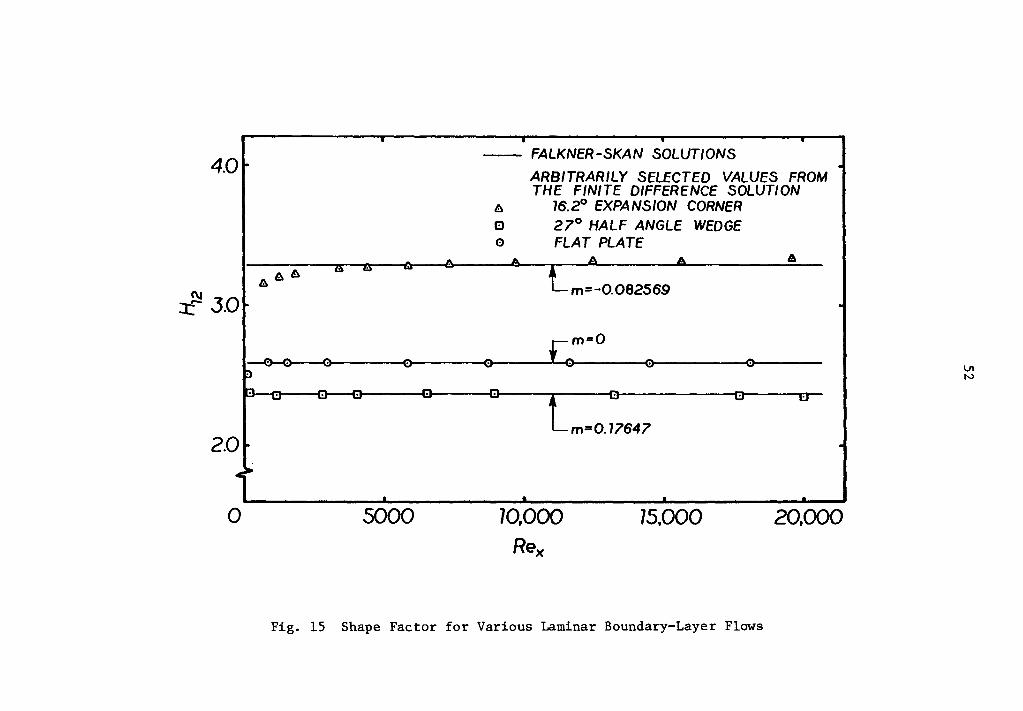
Shape Factor for Various Laminar Boundary-Layer Flows . . . . . . . . . . . . . .
3
9
. • . . . . 13
. . . . 14
19
. . 22
25
42
46 . . . . . . 47 . . . . . . 48 . . . . . . 49 . . . . . . 50 . . . . . . 51 . . . . .
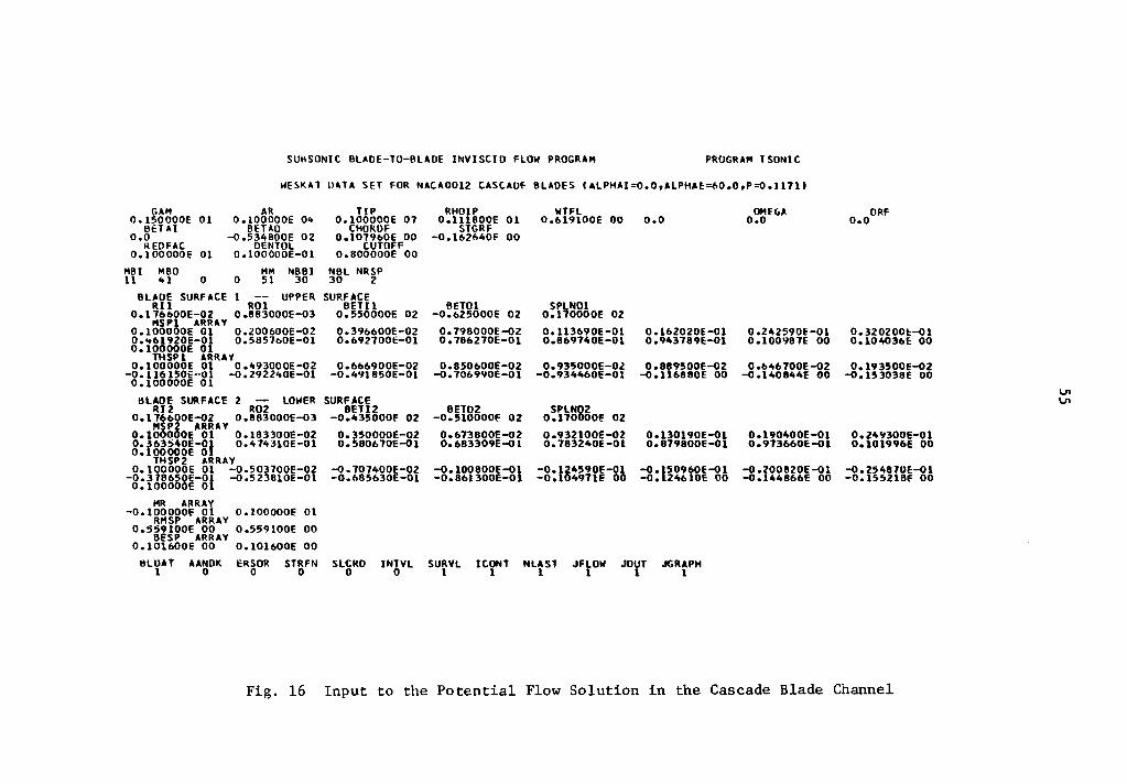
52 . . . . . Input to the Potential Flow Solution in the Cascade Blade Channel . . . . . . . . . . . . . . 55
v
Figure No.
17
18
19
20
21
22
23
24
25
26
27
28
29
Al
List of Figures (continued)
Title
Blade Surf ace Velocities • • • • • • • 5 7
u-Profile for Turbulent Boundary-Layer Flow on a Flat Plate . . . . . •
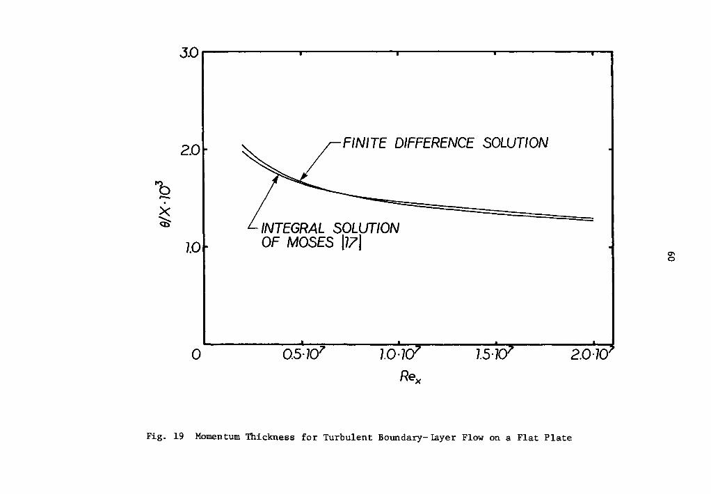
Momentum Thickness for Turbulent Boundary-Layer Flow on a Flat Plate . • . • . . • •
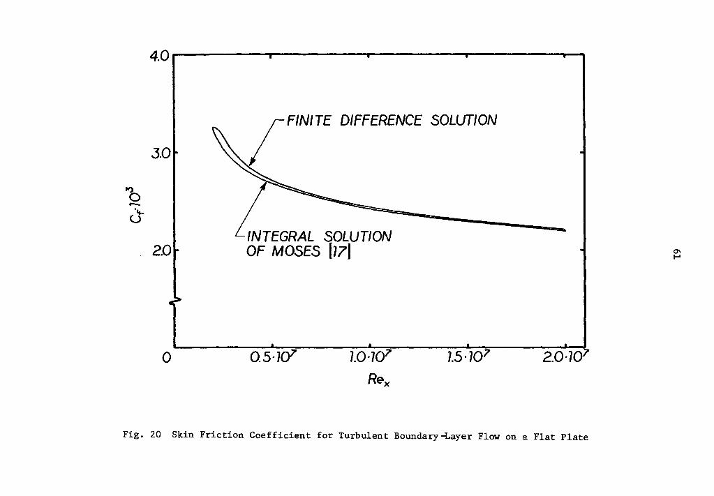
Skin Friction Coefficient for Turbulent Boundary-Layer Flow on a Flat Plate
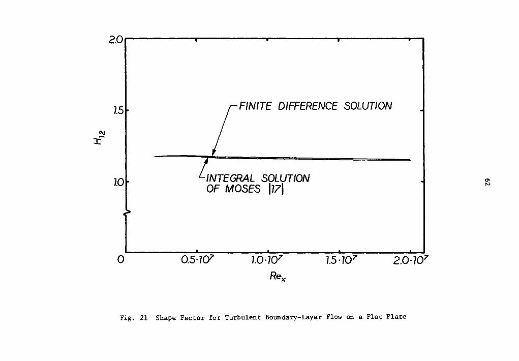
Shape Factor for Turbulent Boundary-Layer Flow on a Flat Plate
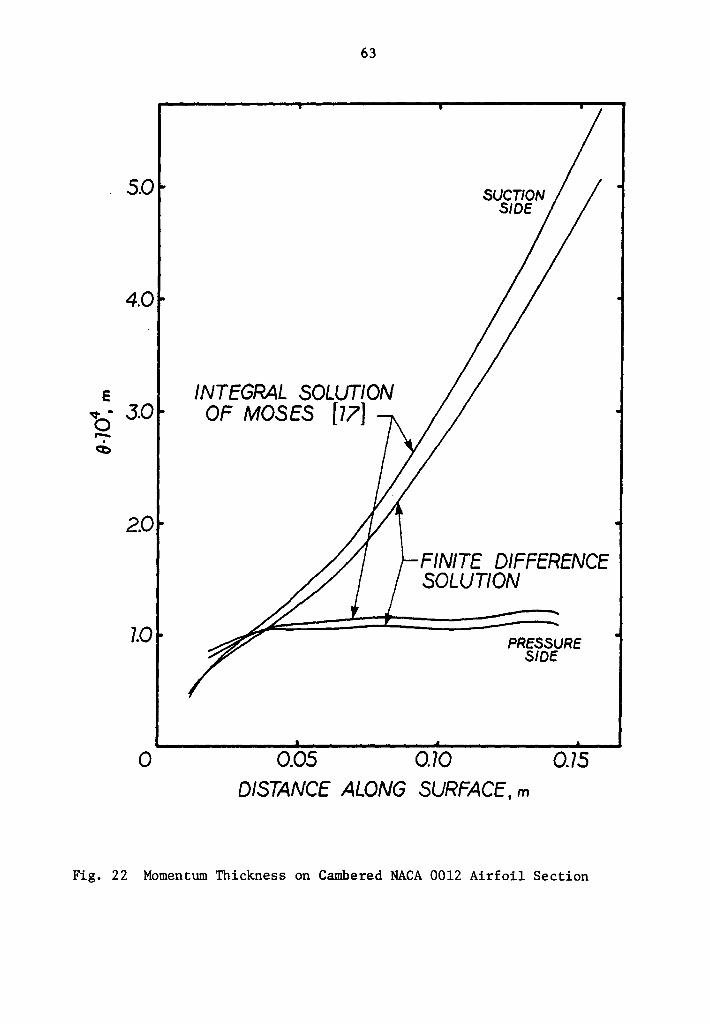
Momentum Thickness on Cambered NACA 0012 Airfoil Section . . . • • . • . . • . .
Skin Friction Coefficient on Cambered NACA 0012 Airfoil Section • • . •
u-Profile on a Flat Plate with Tangential Injection Laminar, oi/s = 0.5, V./u = 1.0
J e
u-Profile on a Flat Plate with Tangential Injection Turbulent, oi/s = 0.5, V./u = 1.0
J e Momentum Thickness on Cambered NACA 0012 Airfoil Section with Tangential Injection Near
59
60
61
62
63
64
66
67
the Leading Edge -- o./s = 0.5, V./u = 1.0 .•.. 69 l. J e
Skin Friction Coefficient on Cambered NACA 0012 Airfoil Section with Tangential Injection Near the Leading Edge -- oi/s = 0.5, V./u = 1.0
J e
u-Profiles on Suction Side of Cambered NACA 0012 Airfoil Section Downstream from Tangential Injection -- o./s = 0.5, V./u = 1.0 ....
l. J e
u-Prof iles on Pressure Side of Cambered NACA 0012 Airfoil Section Downstream from Tangential Injection -- o./s = 0.5, V./u = 1.0 •..
i. J e
Flow Chart for Crank-Nicolson Algorithm
vi
70
71
72
80
Table No.
1
2
3
4
List of Tables
Title
C4, T6, and NACA 0012 Airfoil Sections
Optimum Pitch-Cord Ratio • • . •
Boundary-Layer Edge Conditions
Constants in the Stretching Function
vii
Page
8
10
31
35
A
A , B , C , D n n n n
a
b
c
D
d
e
f
G
1
m
N
p
Nomenclature
van Driest damping factor in the inner-law, eddy-viscosity formulation
Coefficients in the finite-difference form of the boundary-layer momentum equation
Axial length of combustion turbine blade profile
y-intercept of the single-parabolic camberline equation
Skin friction coefficient
Intermediate quantities in the turbulent, two-layer velocity profile
Chord length
Intermediate quantity in the function governing the coordinate transformation
x coordinate of the vertex of the single-parabolic camberline equation
Napierian base
Function resulting from the similarity transformation of the boundary-layer momentum equation
The stretching function
Shape factor
Constant in the edge velocity equation for the laminar flow geometries
Camberline length
(i) Parameter governing the shape of the single-parabolic camberline, or
(ii) pressure gradient parameter
Parameter controlling the amount of "stretching" in the coordinate transformation
(i) Pressure, or (ii) polynomial approximation to the wake function
viii
Re r Re x
s
u
+ u
v
x
y
+ y
a
8
o~ inc
£. 1
£ 0
n
used in the turbulent, two-layer, velocity profile
Reference Reynolds number
Reynolds number based on x
Reynolds number based on o Blade pitch
x-component of velocity
Dimensionless x-component of velocity (= uyp/~ ) w
Wall-jet velocity at initial station
y-component of velocity
Streamwise coordinate
Transverse coordinate
Dimensionless transverse coordinate (= ylT /p/v) w
Constant in stretching function -- from G1 (0)
Inlet blade angle
Exit blade angle
Constant in stretching function -- from G(O)
Boundary layer thickness
Boundary-layer displacement thickness
Incompressible boundary-layer displacement thickness
(i) Eddy viscosity, or (ii) tolerance on the gradient of the u-prof ile
at the boundary-layer edge
Inner eddy-viscosity formulation
Outer eddy-viscosity formulation
(i) Normalized transverse distance, or (ii) similarity variable
ix
8
µ
\)
p
T
Transverse distance at which turbulent velocity profiles switches from inner to outer formulation
Boundary layer momentum thickness
Absolute viscosity
Kinematic viscosity
Density
Total viscosity
Shear stress
Arbitrary function of x and y
Subscripts - Superscripts
Evaluated at the edge th From the i iteration
Evaluated in a linearized manner
Element (m,n) from the boundary-layer grid system
Reference value
Evaluated at the wall
Dimensional quantity
Dimensionless quantity
x
1. Introduction
The objective of the present investigation is the development of
a calculation technique capable of predicting boundary layer velocity
profiles downstream from a tangentially oriented wall jet. The
boundary layer calculation is applied to the steady, two-dimensional,
incompressible, homogeneous flow over representative combustion
turbine blade surfaces. The work has been conducted in coordination
with the Turbomachinery Research Laboratory (TRL) at Virginia.
Polytechnic Institute and State University. The ultimate objective
of this line of research is the determination of the film heat transfer
coefficient for the compressible flow of combustion gases through
turbine blade passages protected by film cooling.
A great deal of engineering effort has been spent in attempts to
increase the thermal efficiency of the combustion turbine. A dual
approach is currently being exercised with research being conducted
on axial flow compressors to reduce the parasitic effect of compressor
power const.nnption and on axial flow turbines to make more power
available for useful work. The trend is toward higher turbine inlet
temperatures on the downstream side of the machines. The American
Society of Mechanical Engineers reports military engine requirements
of alternate operation between 1400 C and 1900 C at the turbine inlet
with high temperature technology being developed for operation in
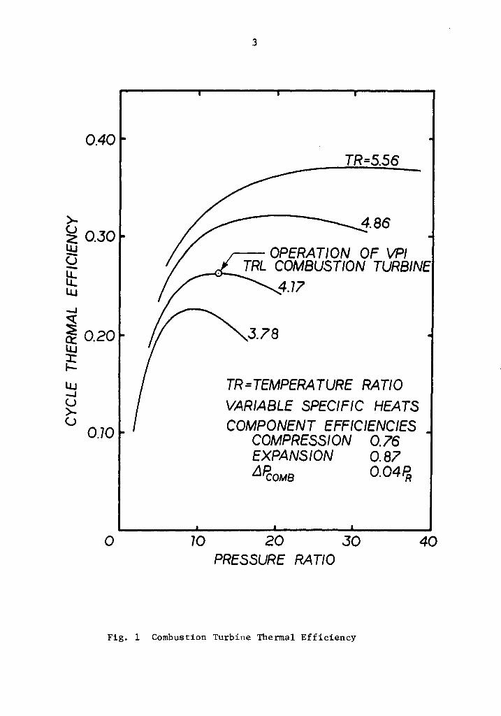
* excess of 2200 C[l]. The effect of increasing the machine temperature
* Numbers in brackets designate References at end of paper.
1
2
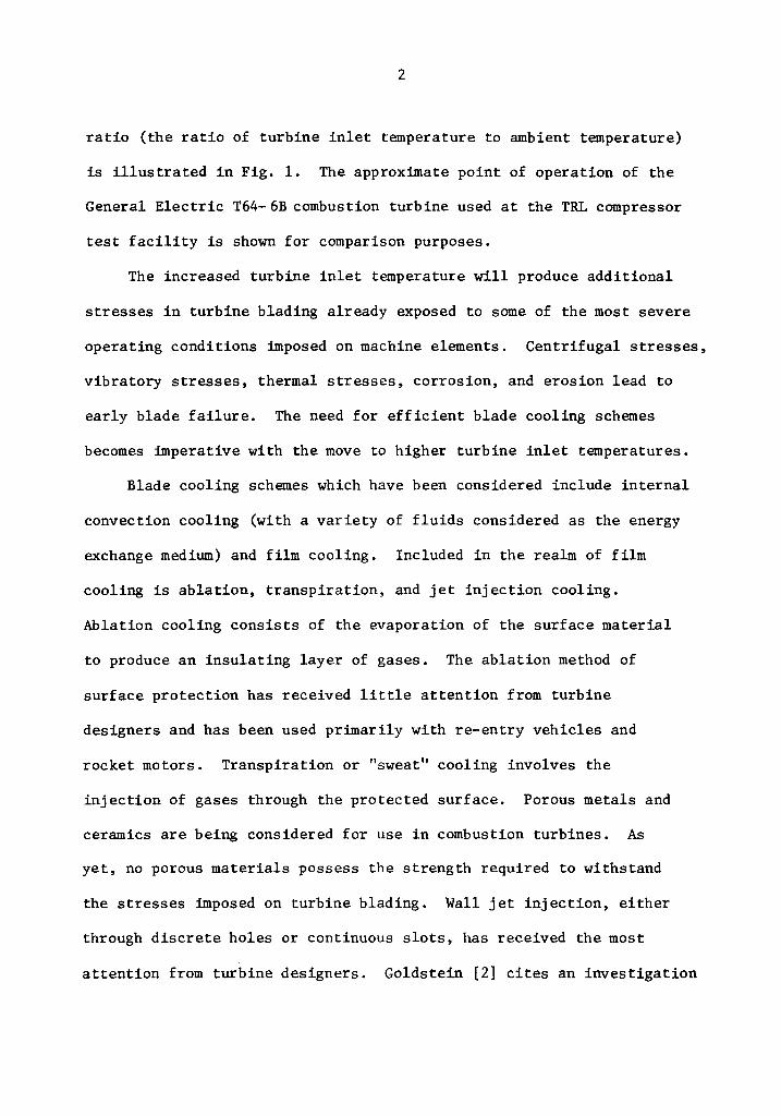
ratio (the ratio of turbine inlet temperature to ambient temperature)
is illustrated in Fig. 1. The approximate point of operation of the
General Electric T64-6B combustion turbine used at the TRL compressor
test facility is shown for comparison purposes.
The increased turbine inlet temperature will produce additional
stresses in turbine blading already exposed to some of the most severe
operating conditions imposed on machine elements. Centrifugal stresses,
vibratory stresses, thermal stresses, corrosion, and erosion lead to
early blade failure. The need for efficient blade cooling schemes
becomes imperative with the move to higher turbine inlet temperatures.
Blade cooling schemes which have been considered include internal
convection cooling (with a variety of fluids considered as the energy
exchange medium) and film cooling. Included in the realm of film
cooling is ablation, transpiration, and jet injection cooling.
Ablation cooling consists of the evaporation of the surface material
to produce an insulating layer of gases. The ablation method of
surface protection has received little attention from turbine
designers and has been used primarily with re-entry vehicles and
rocket motors. Transpiration or "sweat" cooling involves the
injection of gases through the protected surface. Porous metals and
ceramics are being considered for use in combustion turbines. As
yet, no porous materials possess the strength required to withstand
the stresses imposed on turbine blading. Wall jet injection, either
through discrete holes or continuous slots, has received the most
attention from turbine designers. Goldstein [2] cites an investigation
0.40
)..
~ 0 . .30 UJ D -It Lu -J
~ a: 0.20 Lu ~ Lu -J (..) ).. (..)
0.70
0
3
TR=5.56
-- OPERATION OF VP/ TRL COMBUSTION TURBINE
TR=TEMPERATURE RATIO VARIABLE SPECIFIC HEATS COMPONENT EFFICIENCIES
COMPRESSION 0.76 EXPANSION 0.87 LlPcoMB 0.04~
10 20 JO PRESSURE RATIO
40
Fig. 1 Combustion Turbine Thermal Efficiency
4
by Eckert and Livingood in which the most efficient use of a unit of
coolant was determined to be internal convection cooling with jet
injection into the stream.
The reports of Goldstein [2], and Beckwith and Bushnell [3]
serve as adequate literature reviews in the field of film cooling.
Goldstein reports in detail the work of numerous investigators,
concentrating on film cooling through wall jet injection. Various
injection geometries and combinations of free-stream and injected
stream fluids yielding non-homogeneous flows are presented. Beckwith
and Bushnell deal with wall jet injection in supersonic flow. Their
investigation is directed toward cooling re-entry and supersonic flight
vehicles.
One of the earliest and perhaps most significant attempts at
predicting wall jet behavior is by Glauert [4]. Glauert developed
similarity solutions for laminar and turbulent wall jets spreading
either radially or two-dimensionally over a surface. Glauert's study
applies to wall jet flow with a zero velocity free stream.
McGahan [5] attacked the wall jet flowing in the presence of a
zero velocity free stream and in the presence of an adverse pressure
gradient. He used a five parameter integral analysis which required
approximations for the shear stress at five locations in the boundary
layer for the adverse pressure gradient case.
More exotic techniques by Beckwith and Bushnell [3], Miner [6],
and Levine [7] attempt to calculate the behavior of the wall jet in
supersonic, reacting flows.
5
The present investigation has been conducted in two parts. The
first portion was spent developing a turbine vane profile representative
of modern combustion turbines. The second, and most lengthy portion
of the investigation dealt with the development of a finite difference
calculation to predict the interaction of a wall jet with some
initial boundary layer development which had occurred on the blade
surfaces up to the point of injection. The calculation was verified
by comparison of predicted results with results from well-known
solutions for both laminar and turbulent boundary layer flows.
The following discussion begins with a description of the
method used to generate the turbine vane profile. The boundary
layer analysis follows. The equations governing conservation of
mass and momentum in the boundary layer are adapted to the finite-
difference grid used in the solutions. Included are descriptions
of the boundary conditions, the eddy viscosity model used in the
turbulent flow calculations, and the wall-jet model at the point of
injection into the boundary layer.
2. Turbine Blade Geometry
The selection of efficient airfoil sections is important to
aerodynamicists and combustion turbine designers. "Airfoil
efficiency" is a function of many parameters where the specific
application of the airfoil must be defined before the optimtun
airfoil shape can be selected. The blade shape of interest to
turbine designers is one which will accept the flow at a given
incidence angle and turn the flow through the required deflection
angle with minimum frictional losses. Frictional losses in a blade
channel include the effects of profile loss, annulus loss, secondary
flow loss, and tip clearance loss. Turbine designers lump these
effects into the overall blade loss coefficient [8].
The flow considered in this investigation is analogous to the flow
through a two-dimensional cascade. Thus, the overall loss coefficient
consists of profile losses only.
Airfoil sections are specified by describing a thickness form
and a camber line form. The thickness form is a description of the
blade surface height relative to a straight, or zero camber, mean
blade line. The thickness form may or may not be symmetric about the
mean blade line. The camber line form is a description of the
deviation of the actual mean blade line from the zero camber mean
blade line. Jacobs [9] states that the thickness form primarily
dictates the structural character~stics of the blade while the
camber line form controls the important aerodynamic characteristics
of an airfoil section.
6
7
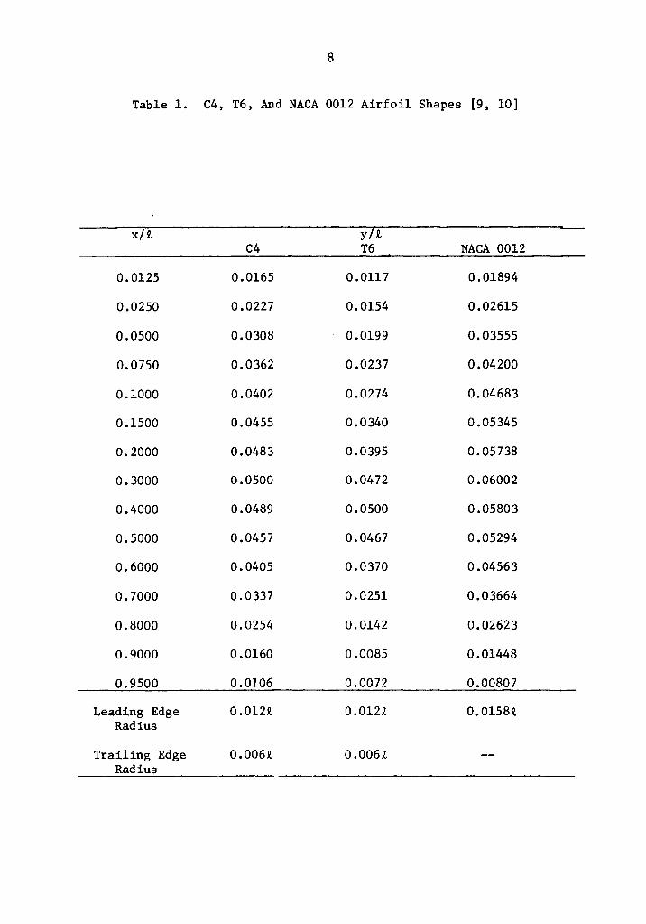
The thickness forms which are commonly used for turbine blading
include the C4, T6, and NACA 0012 base profiles. The C4 base profile
is of British origin while the T6 and NACA 0012 base profiles were
developed in the American combustion turbine industry. The C4,
T6, and NACA 0012 base profiles are given in Table 1 where the blade
surface height is a function of the camber line length. All profiles
listed are symmetric about the mean line.
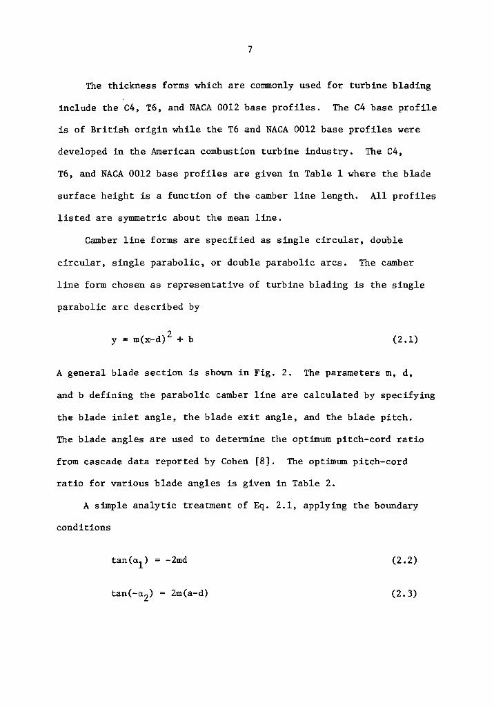
Camber line forms are specified as single circular, double
circular, single parabolic, or double parabolic arcs. The camber
line form chosen as representative of turbine blading is the single
parabolic arc described by
y = m(x-d) 2 + b (2.1)
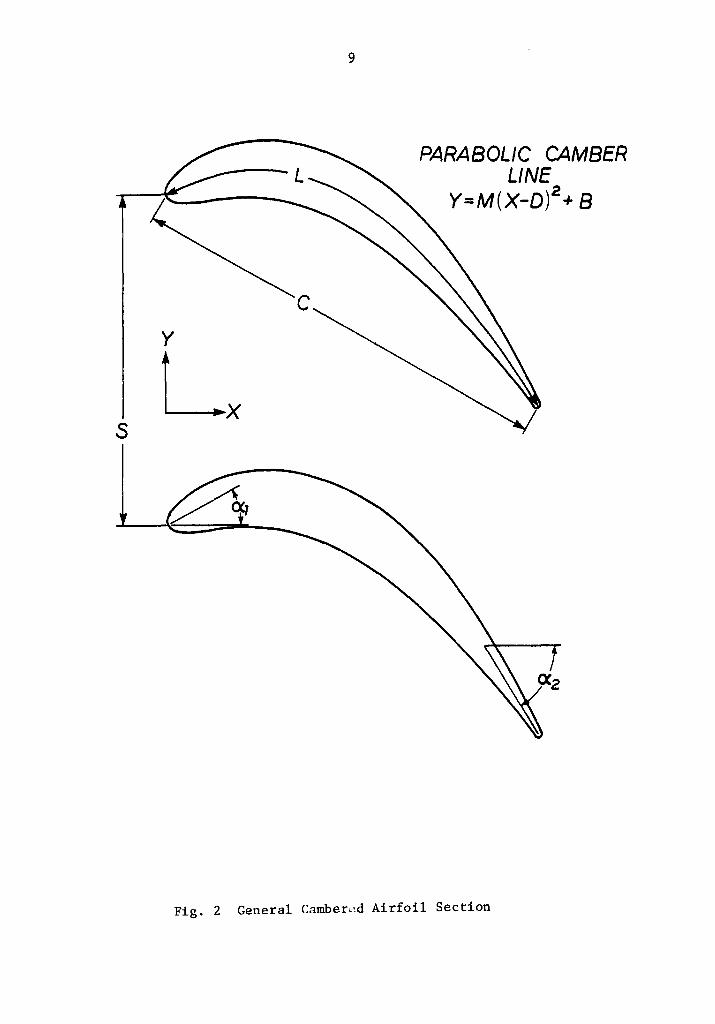
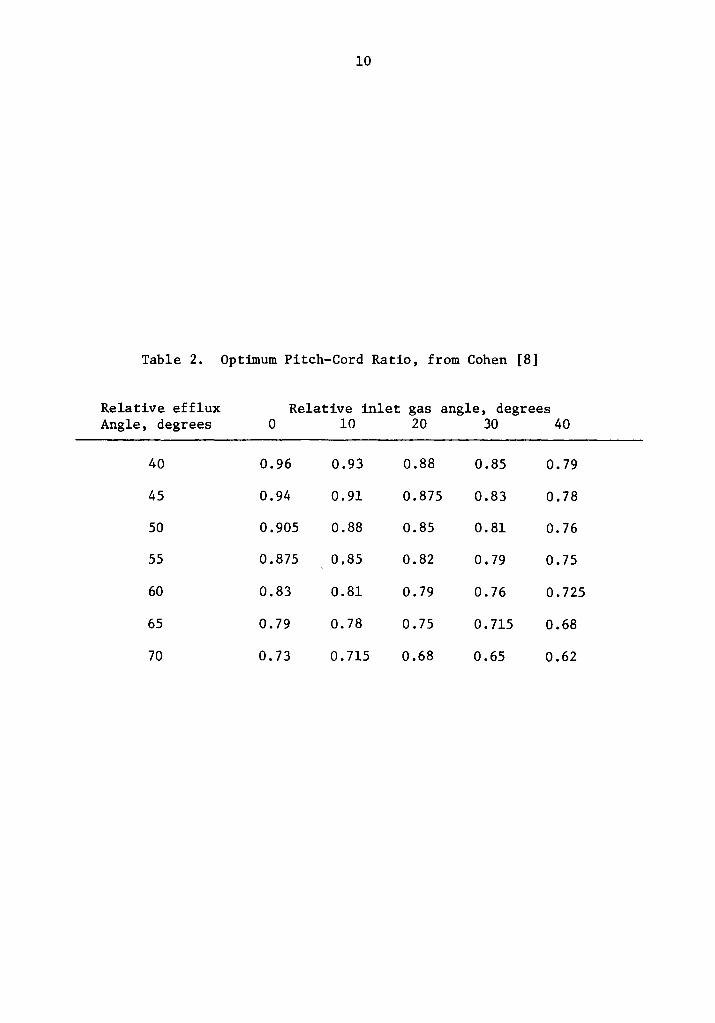
A general blade section is shown in Fig. 2. The parameters m, d,
and b defining the parabolic camber line are calculated by specifying
the blade inlet angle, the blade exit angle, and the blade pitch.
The blade angles are used to determine the optimum pitch-cord ratio
from cascade data reported by Cohen [8). The optimtml pitch-cord
ratio for various blade angles is given in Table 2.
A simple analytic treatment of Eq. 2.1, applying the boundary
conditions
(2.2)
2m(a-d) (2.3)
8
Table 1. C4, T6, And NACA 0012 Airfoil Shapes [9, 10]
x/9., y/9., C4 T6 NACA 0012
0.0125 0.0165 0.0117 0.01894
0.0250 0.0227 0.0154 0.02615
0.0500 0.0308 0.0199 0.03555
0.0750 0.0362 0.0237 0.04200
0.1000 0.0402 0.0274 0.04683
0.1500 0.0455 0.0340 0.05345
0.2000 0.0483 0.0395 0.05738
0.3000 0.0500 0.0472 0.06002
0.4000 0.0489 0.0500 0.05803
0.5000 0.0457 0.0467 0.05294
0.6000 0.0405 0.0370 0.04563
0.7000 0.0337 0.0251 0.03664
0.8000 0.0254 0.0142 0.02623
0.9000 0.0160 0.0085 0.01448
0.9500 0.0106 0.0072 0.00807
Leading Edge 0. 0129., 0.012!1, 0.01589., Radius
Trailing Edge 0.006!1, 0.0069., Radius
s
9
PARABOLIC CAMBER LINE
Y=M(X-0)2 + B
Fig. 2 General CamberL~d Airfoil Section
10
Table 2. Optimum Pitch-Cord Ratio, from Cohen [8]
Relative efflux Relative inlet gas angle, degrees Angle, degrees 0 10 20 30 40
40 0.96 0.93 0.88 0.85 0.79
45 0.94 0.91 0.875 0.83 0.78
50 0.905 0.88 0.85 0.81 0.76
55 0.875 0.85 0.82 0.79 0.75
60 0.83 0.81 0.79 0.76 o. 725
65 0.79 0.78 0.75 o. 715 0.68
70 0.73 o. 715 0.68 0.65 0.62
11
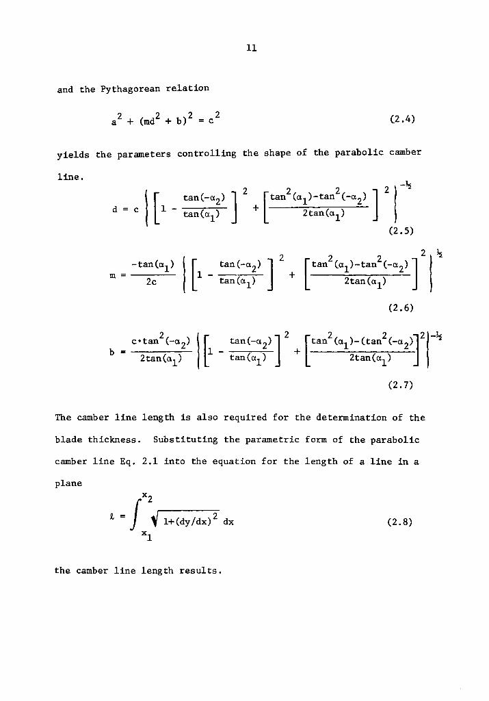
and the Pythagorean relation
(2 .4)
yields the parameters controlling the shape of the parabolic camber
line.
d =
m =
b =
-~
c I [ 1 _ tan(-a.2) ] 2 2 2 + [tan (a1 )-tan (-a2) r tan(a1)
-tan(a.1 )
2c
2 c•tan (-a. 2)
2tan(a.1)
[1 -tan(-a.2) ] tan (a.1)
2tan(a.1)
(2. 5)
2 [tan
2(a1 )-tan
2(-a2)]
+ 2tan(a.1)
(2. 6)
(2. 7)
2
The camber line length is also required for the determination of the
blade thickness. Substituting the parametric form of the parabolic
camber line Eq. 2.1 into the equation for the length of a line in a
plane
(2.8)
the camber line length results.
~
12
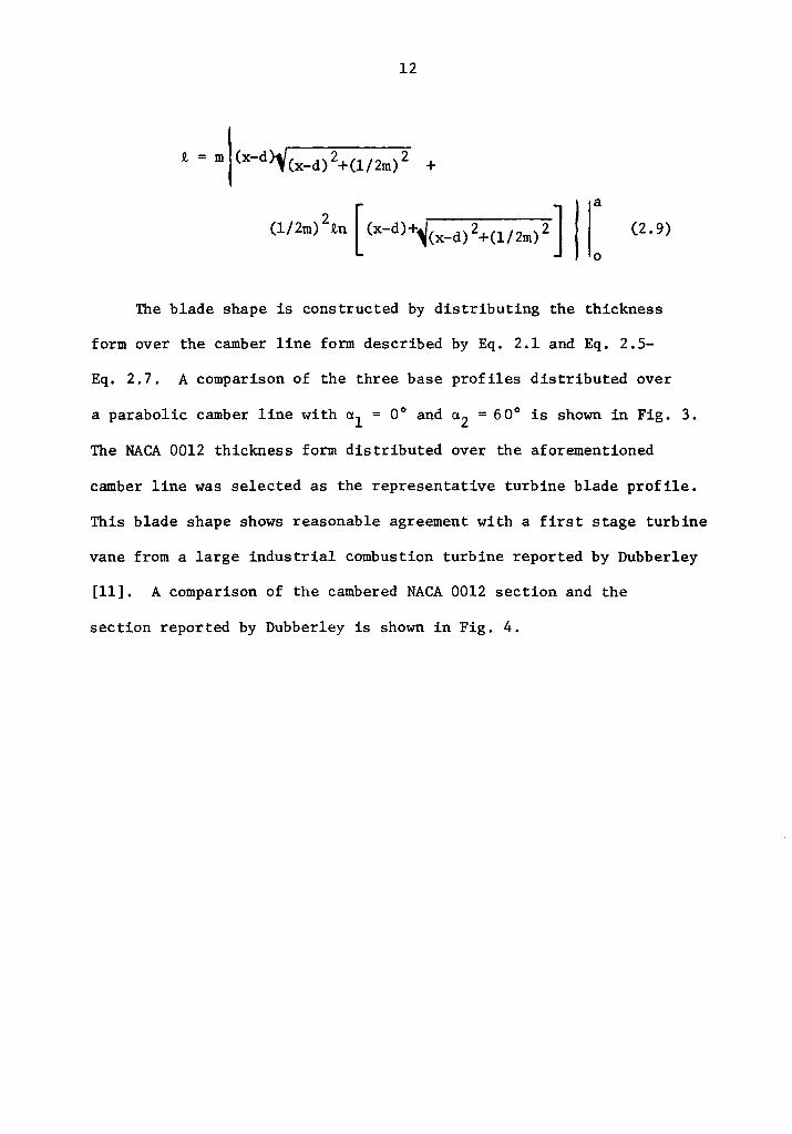
(2.9)
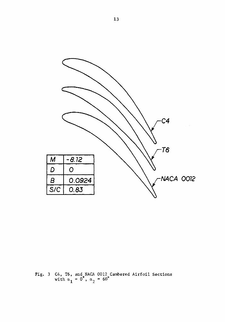
The blade shape is constructed by distributing the thickness
form over the camber line form described by Eq. 2.1 and Eq. 2.5-
Eq. 2.7. A comparison of the three base profiles distributed over
a parabolic camber line with a1 = 0° and a2 = 60° is shown in Fig. 3.
The NACA 0012 thickness form distributed over the aforementioned
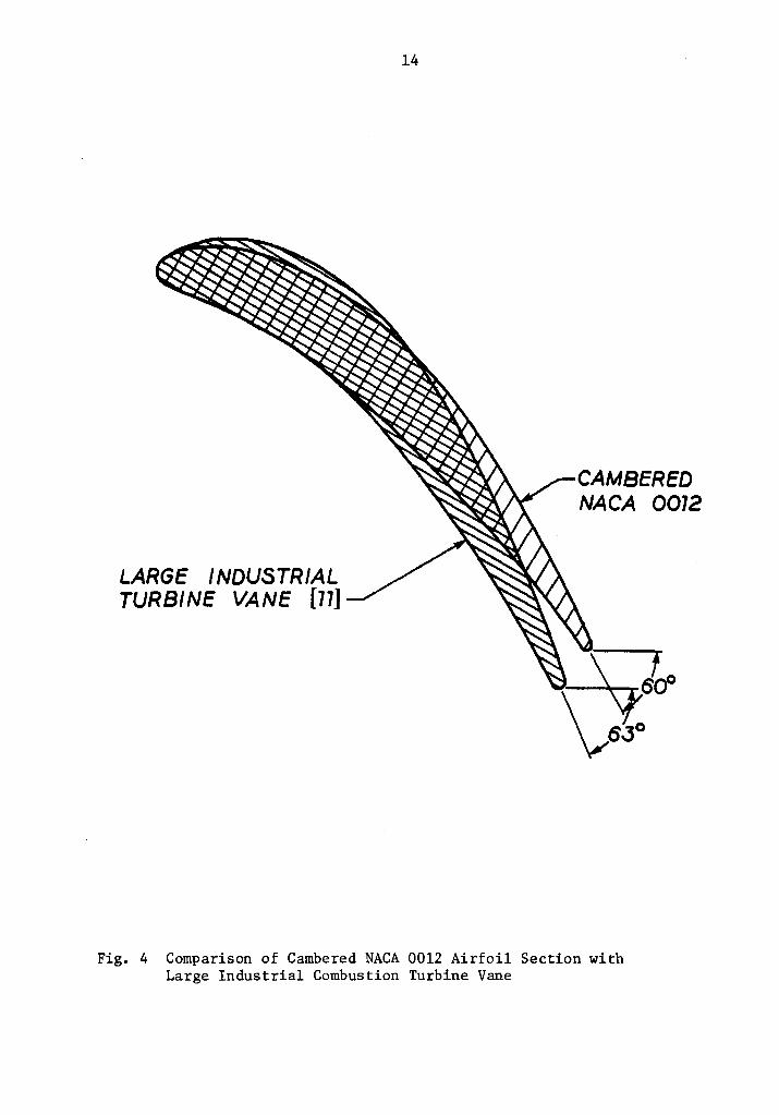
camber line was selected as the representative turbine blade profile.
This blade shape shows reasonable agreement with a first stage turbine
vane from a large industrial combustion turbine reported by Dubberley
[11]. A comparison of the cambered NACA 0012 section and the
section reported by Dubberley is shown in Fig. 4.
13
C4
T6 M -8.12 D 0 B 0.0924 NACA 0012 SIC 0.83
Fig. 3 C4, T6, and NACA 0012 Cambered Airfoil Sections with a 1 = 0°, a 2 = 60°
LARGE INDUSTRIAL TURBINE VANE [77]
14
CAMBERED NACA 0072
Fig. 4 Comparison of Cambered NACA 0012 Airfoil Section with Large Industrial Combustion Turbine Vane
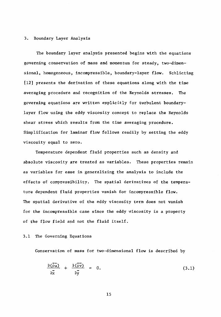
3. Boundary Layer Analysis
The boundary layer analysis presented begins with the equations
governing conservation of mass and momentum for steady, two-dimen-
sional, homogeneous, incompressible, boundary-layer flow. Schlicting
[12) presents the derivation of these equations along with the time
averaging procedure and recognition of the Reynolds stresses. The
governing equations are written explicitly for turbulent boundary-
layer flow using the eddy viscosity concept to replace the Reynolds
shear stress which results from the time averaging procedure.
Simplification for laminar flow follows readily by setting the eddy
viscosity equal to zero.
Temperature dependent fluid properties such as density and
absolute viscosity are treated as variables. These properties remain
as variables for ease in generalizing the analysis to include the
effects of compressibility. The spatial derivatives of the tempera-
ture dependent fluid properties vanish for incompressible flow.
The spatial derivative of the eddy viscosity term does not vanish
for the incompressible case since the eddy viscosity is a property
of the flow field and not the fluid itself.
3.1 The Governing Equations
Conservation of mass for two-dimensional flow is described by
a(pu) ax +
a(pv) ay = o. (3.1)
15
16
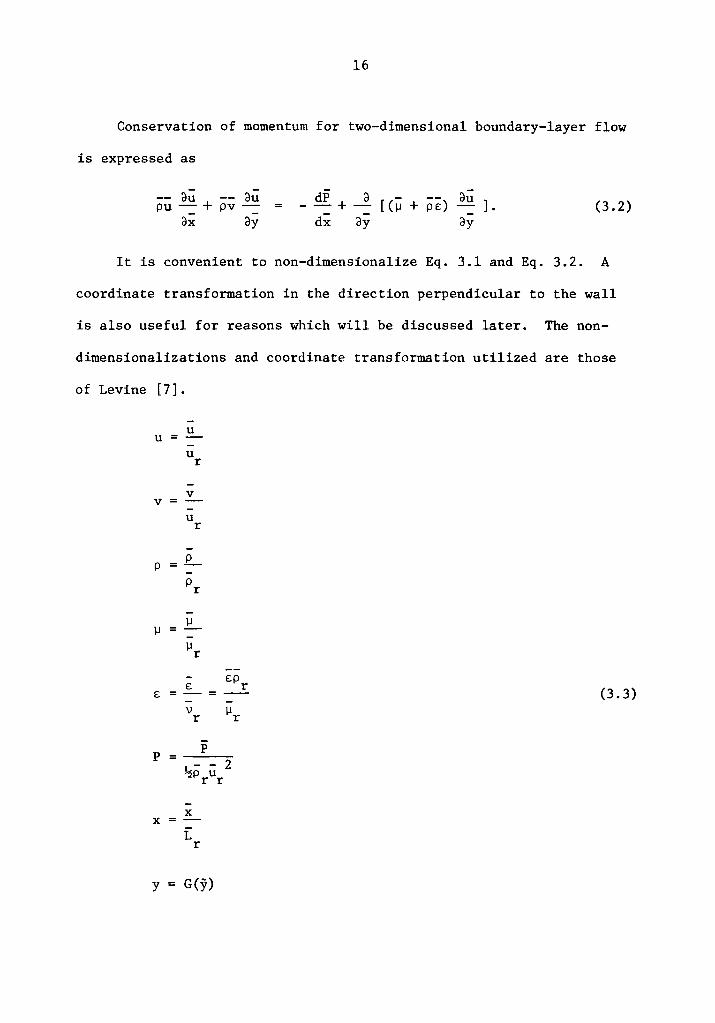
Conservation of momentum for two-dimensional boundary-layer flow
is expressed as
-- au au PU - + pv-:-
ax ay _ dP + ~ [<ii + f)£) au l . (3.2) dx ay
It is convenient to non-dimensionalize Eq. 3.1 and Eq. 3.2. A
coordinate transformation in the direction perpendicular to the wall
is also useful for reasons which will be discussed later. The non-
dimensionalizations and coordinate transformation utilized are those
of Levine (7].
u u = -u r
v v u r
p = _e_ Pr
µ µ = µr
e: e:pr (3.3) e: =- =
\) µr r
p p
~p u 2 2 r r
x x = -L r
y = G(y)
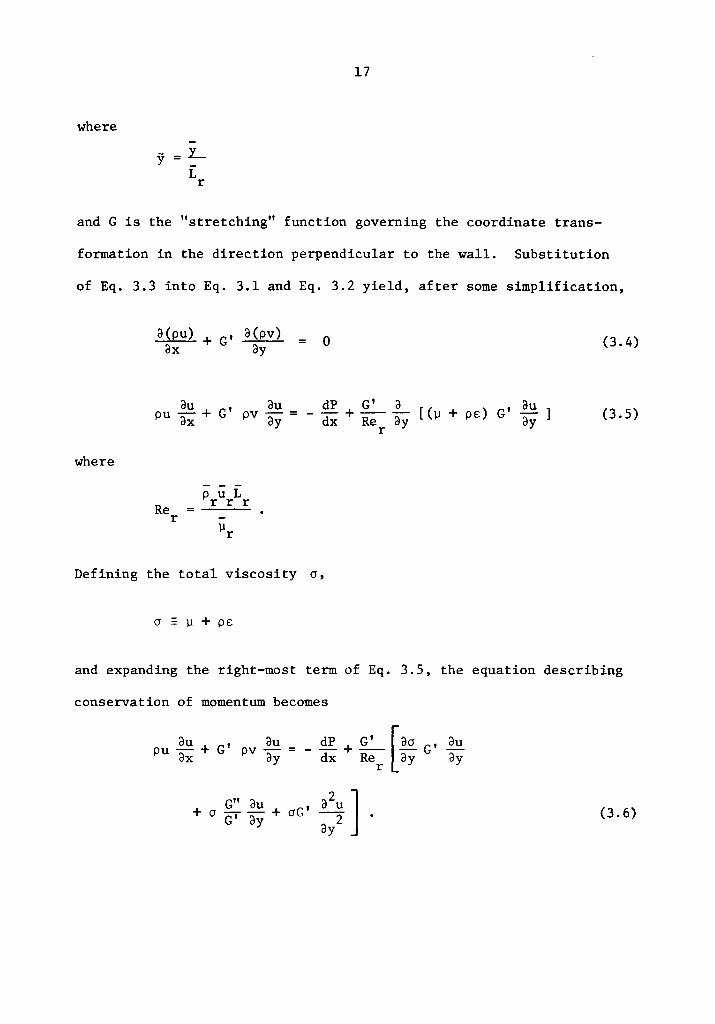
where
y =L L r
17
and G is the "stretching" function governing the coordinate trans-
formation in the direction perpendicular to the wall. Substitution
of Eq. 3.3 into Eq. 3.1 and Eq. 3.2 yield, after some simplification,
where
a(pu) + G' a(pv) ax ay 0
p u ~ + GI pv au = - dP + ~ .2..__ [ ( µ + p £) GI au ax ay dx Re ay ay
Re r
r
Defining the total viscosity o,
cr - µ + P£
(3.4)
(3.5)
and expanding the right-most term of Eq. 3.5, the equation describing
conservation of momentum becomes
PU ~ + GI pv au = - dP + ~ [~ GI au ax ay dx Re ay ay
r
G" au I a2u J + cr G' ay + oG --2 •
ay (3.6)
18
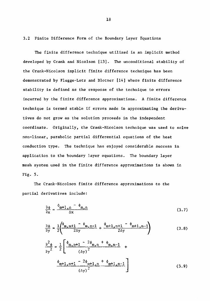
3.2 Finite Difference Form of the Boundary Layer Equations
The finite difference technique utilized is an implicit method
developed by Crank and Nicolson [13]. The unconditional stability of
the Crank-Nicolson implicit finite difference technique has been
demonstrated by Flugge-Lotz and Blotner [14] where finite difference
stability is defined as the response of the technique to errors
incurred by the finite difference approximations. A finite difference
technique is termed stable if errors made in approximating the deriva-
tives do not grow as the solution proceeds in the independent
coordinate. Originally, the Crank-Nicolson technique was used to solve
non-linear, parabolic partial differential equations of the heat
conduction type. The technique has enjoyed considerable success in
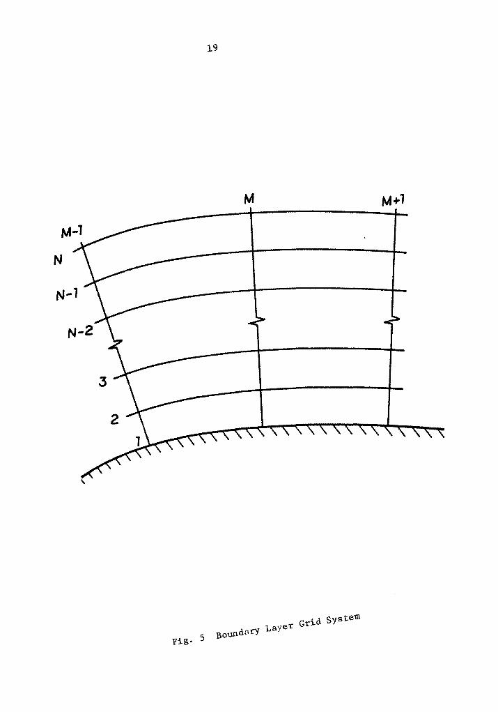
application to the boundary layer equations. The boundary layer
mesh system used in the finite difference approximations is shown in
Fig. 5.
The Crank-Nicolson finite difference approximations to the
partial derivatives include:
a~ ¢m+l,n - ~m,n ax= t!,x
it= 1.(~m,n+l - ~m,n-1 + ~m+l,n+l - ~m+l,n-1\ ay 2 2r:,y 2r:,y I ~ = .!.[~m,n+l - 2 ~m,n + ~m,n-1 + ay2 2 (t:,y)2
~m+l,n+l - 2~m+l,n + ~m+l,n-1 J (t.y) 2
(3. 7)
(3.8)
(3.9)
19
M
\
20
where <f> is some arbitrary function of x and y. Letting
<Py <Pm,n+l - <Pm 2n-l
2fly
and
<Pm,n+l - 2<f> + <Pm n-1 <Pyy =
m,n ' (fly) 2
Eq. 3.8 and Eq. 3.9 may be expressed in a somewhat more concise form.
~ = .! <I> + m+l,n+l m+l,n-1 (
<I> -<P ) ay 2 y 2fly
a2<1> 1 [<I> + <Pm+l,n+l - 2<1>m+l,n + <Pm+l,n-1] ay2 = 2 yy (fly)2
Replacing the arbitrary function <I> by u in Eq. 3.7, Eq. 3.10, and
Eq. 3.11, substituting these approximations into Eq. 3.6, and
simplifying yields
A u + B u + C u = D n m+l,n+l n m+l,n n m+l,n-1 n
where the coefficients A , B , C , and D are given by n n n n
A = n
B = n (pu)t
flx
G' [aa G' + aG" J __ a_G_,_2 __ - 4Rerfly ay G' 2Re (fly)2
r
+ aG' 2
(fly)2
c (pv)tG'
+ G' [l<'.c• aG" J aG 12 = - +-- -n 46y 4Rerfly ay G' 2Re (fly) r
2
(3.10)
(3.11)
(3 .12)
(3.13)
(3 .14)
(3 .15)
D n
(pu) 1u u ___ m~, n_ + _:t_ /j,x 2
0G 12u dP + yy dx 2Re
r
21
[~. Re r
(3.16)
The Crank-Nicolson finite difference approximations lead to the
solution of the momentum equation about the point (m+1~ 2 n) as shown
in Fig. 6. The momentum equation at each downstream location is
represented by Eq. 3.12. Solution to the momentum equation at each
downstream location is affected by solving the system of equations
represented by Eq. 3.12. This system of equations constitutes a
linear system of algebraic equations if the coefficients A through n
D are not functions of the u velocities at the downstream locations. n
The mass flux terms, pu and pv, and the total viscosity, o, must
therefore be linearized so that the system of equations may be solved.
The solution of the momentum equation about the m+1~ points lends
itself readily to linearization. The mass flux terms and the total
viscosity at the ~ stations are thus approximated by
<I> (i+l) m+1~,n
1 (<I> + <l>(i) ) 2 m,n m+l,n
where the superscripts in the above equation imply an iterative
process. The quantities at the (m+l)st station are first assumed
equivalent to the quantities at the mth station. The system of
(3.17)
equations represented by Eq. 3.12 is then solved to obtain a better
estimate to the values at station m+l. The new estimates are then
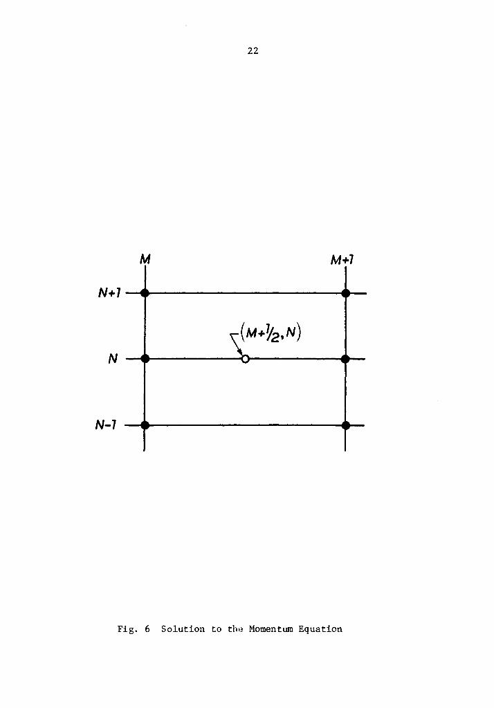
22
M M+7
N -
N-7
Fig. 6 Solution to the Momentum Equation
23
used in Eq. 3.17 as approximations to the values at m+l. The averaging
process is repeated, the system of equations solved, and a new esti-
mate to the values at m+l obtained until the process converges. In
general, it was assumed that the solution had converged when u(i+ll) m+ ,n (i)
was within 1 per cent of um+l,n'
according to Clausing [15], is to (i)
an acceptable tolerance of vm+l,n'
A more strict convergence criteria,
bring the value of v(i+l) to within m+l,n
The highly structured nature of the system of equations
represented by Eq. 3.12 may be utilized in implementing the simul-
taneous solution technique. Inspection of Eq. 3.12 reveals that the
coefficient matrix is tri-diagonal. The tri-diagonal system of
equations contains n-2 equations in n-2 unknowns, u2 through un-l'
The extreme nodes, u1 and un' are given by the edge conditions
governing the boundary-layer flow.
The algorithm used to solve a tri-diagonal system of equations
is one of forward elimination and back substitution. The first
equation of the system, containing the three nodes nearest to the
wall, is solved explicitly for the diagonal term. The sub-diagonal
term of the first equation c2u1 , is known from the boundary condition
at the wall and may be incorporated into n2 . The result is sub-
stituted into the second equation for the sub-diagonal term. This
equation is then solved explicitly for the diagonal term. The
substitution process continues until the (n-2)nd equation of the
system is solved explicitly for the diagonal term. The super-diagonal
term, A 1u , is known from the boundary condition at the freestream n- n
24
edge of the boundary layer and is incorporated into D 1 . The n-
substitution process is essentially one of forward elimination in
which the sub-diagonal term of each equation is eliminated and the
diagonal term is expressed in terms of the super-diagonal term and
lesser coefficients. The result of the forward elimination procedure
is an explicit expression for the (n-2)nd unknown in terms of the
coefficients Ai through Di, i = 2,3,4, ... n-l. Once a value for the
(n-2)nd unknown has been calculate~ it may be back substituted into
the expressions for the diagonal terms to obtain a complete solution
to the system of equations.
The finite difference form of the equation governing conservation
of mass, Eq. 3.4, is constructed for solution about the point shown
in Fig. 7. The approximations to the partial derivatives in Eq. 3.4
are:
~ = l-_ (<Pm+l,n -ax 2 fix
<Pm,n + <Pm+l,n-1 -fix
acp <Pm+l,n - <Pm+l,n-1 Cly = fiy
•m,n-1) (3.18)
(3 .19)
Pierce [16] argues that the finite difference approximation to Clcp/Cly,
Eq. 3.10, applied to the solution of the mass conservation equation
leads to an unstable solution. Early in the analysis it was observed
that for zero pressure gradient flow the approximation to Cl(pv)/ay
given by Eq. 3.10 produced negative y velocities -- a violation of
the physics of the flow. Equation 3.19, recommended by Pierce,
produced acceptable results for the zero pressure gradient case and
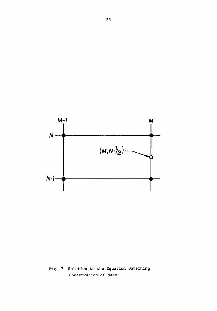
25
M-1 M
N--4.------------~~
N-1~-----------.111~
Fig. 7 Solution to the Equation Governing Conservation of Mass
26
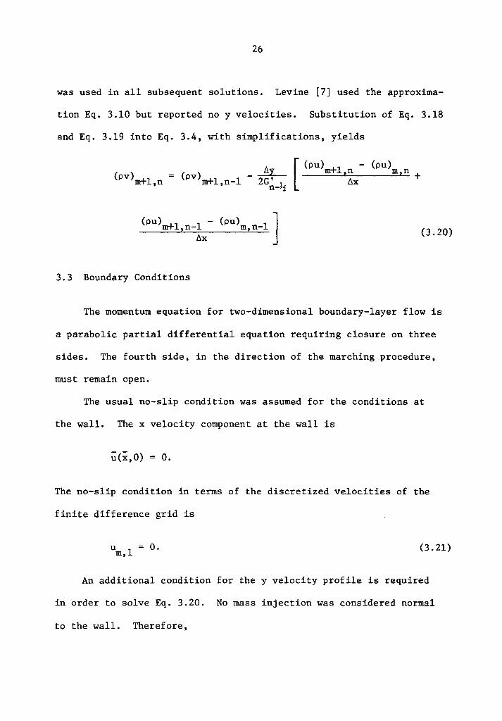
was used in all subsequent solutions. Levine [7] used the approxima-
tion Eq. 3.10 but reported no y velocities. Substitution of Eq. 3.18
and Eq. 3.19 into Eq. 3.4, with simplifications, yields
(pv)m+l,n = ( D.y [ (pu)m+l,n - (pu)m,n +
pv)m+l,n-1 - 2G' b.x n-!2
(pu)m+l,n-1 - (pu)m,n-1] b.x
3.3 Boundary Conditions
(3.20)
The momentum equation for two-dimensional boundary-layer flow is
a parabolic partial differential equation requiring closure on three
sides. The fourth side, in the direction of the marching procedure,
must remain open.
The usual no-slip condition was assumed for the conditions at
the wall. The x velocity component at the wall is
il<x,o) = o.
The no-slip condition in terms of the discretized velocities of the
finite difference grid is
u 1 = o. m, (3. 21)
An additional condition for the y velocity profile is required
in order to solve Eq. 3.20. No mass injection was considered normal
to the wall. Therefore,
27
v(i,O) O.
In terms of the finite difference grid, the above becomes
v = o. m,l
Mass injection normal to the wall, as is the case with a porous
(3.22)
surface, would imply some v 1 = v(x) and could be incorporated into m,
the analysis.
Initial velocity profiles must be specified to start the calcu-
lation. Boundary layer calculations are typically started at the edge
of the stagnation flow region. Most of the flow geometries invest!-
gated had no well defined stagnation region so alternate models for
the initial profiles were used. The initial velocity profiles for both
laminar and turbulent flow were assumed to be equivalent to those
profiles which would develop on a flat plate in the same axial
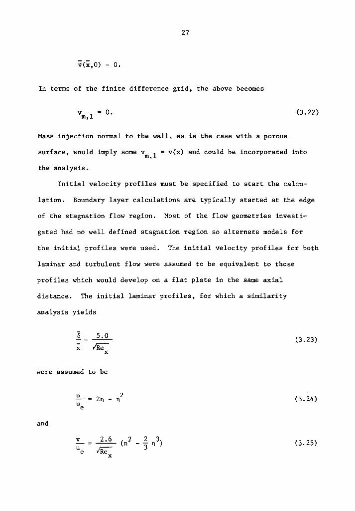
distance. The initial laminar profiles, for which a similarity
analysis yields
6 5.0 - = (3. 23) x ~ x
were assumed to be
u 2n - 2 -= n (3. 24) u e
and
v 2.6 (n 2 2 3 -= - - n ) u ~ 3 e (3.25)
x
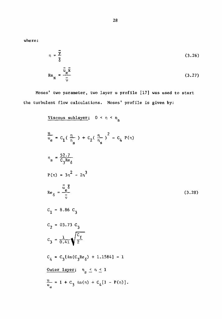
where:
n = y
Re x
6
u x e
\)
28
(3. 26)
(3.27)
Moses' two parameter, two layer u profile [17] was used to start
the turbulent flow calculations. Moses' profile is given by:
Viscous sublayer; 0 < n < ns
u u c ( .!l._ ) + c ( .!l._ ) e 1 n 2 n s s
52.7 n = s c3Re 0
P(n) = 3n 2 - 2n 3
ii 8 Re 0
e =--\)
cl 8.86 c3
c 2 = 03.73 c 3
c3 ~ 0\1~
Outer layer; n < n < 1 s- -
2 - c4 P(n)
~ = 1 + c 3 ~n(n) + c4[1 - P(n)]. e
(3.28)
29
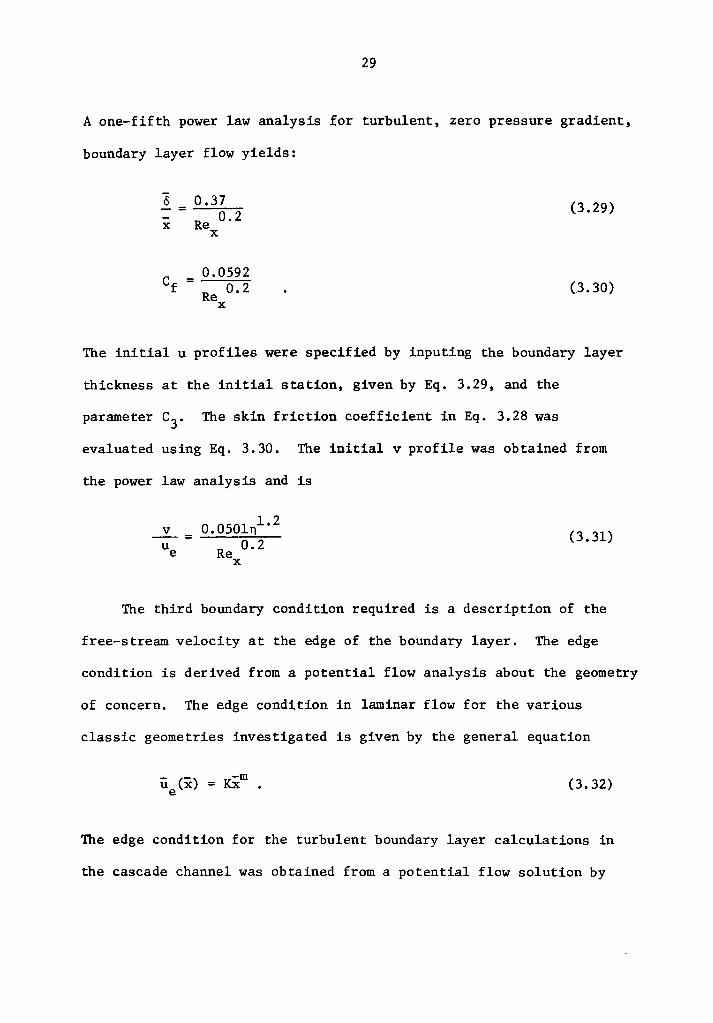
A one-fifth power law analysis for turbulent, zero pressure gradient,
boundary layer flow yields:
8 0.37 - = Re 0.2 x
(3.29) x
cf 0.0592 = Rex
0.2 (3.30)
The initial u profiles were specified by inputing the boundary layer
thickness at the initial station, given by Eq. 3.29, and the
parameter c3. The skin friction coefficient in Eq. 3.28 was
evaluated using Eq. 3.30. The initial v profile was obtained from
the power law analysis and is
v --= 0.050lnl. 2
Re 0.2 x
(3.31)
The third boundary condition required is a description of the
free-stream velocity at the edge of the boundary layer. The edge
condition is derived from a potential flow analysis about the geometry
of concern. The edge condition in laminar flow for the various
classic geometries investigated is given by the general equation
ii ex> e -m = K.x • (3. 32)
The edge condition for the turbulent boundary layer calculations in
the cascade channel was obtained from a potential flow solution by
30
Katsanis [18]. A summary of the boundary layer edge conditions is
given in Table 3.
It is impractical to supply a discrete edge condition for each
downstream location due to the large number of finite difference steps
needed to proceed in the downstream direction. A method of inter-
polation was sought which would adequately describe the edge velocity
and edge velocity gradient using a minimum number of data points.
The edge velocity and edge velocity gradient are used in the Bernoulli
relation
dP dx (3.33)
to determine the pressure gradient driving the boundary layer flow.
Cubic spline interpolation using the "free end" condition was chosen
as the interpolation technique. This method has a significant
advantage over nth order polynomial interpolation. The derivative
of the cubic spline interpolating polynomial may be used to describe
the edge velocity gradient. No finite difference technique is
required to calculate the pressure gradient. Ahlberg (19] discusses
the utility of the cubic spline as an approximation technique.
One additional boundary condition is required to control the
boundary layer thickness and the number of mesh nodes in the y
direction. The criterion for the u velocity gradient at the boundary
layer edge is
au. ay
= o.
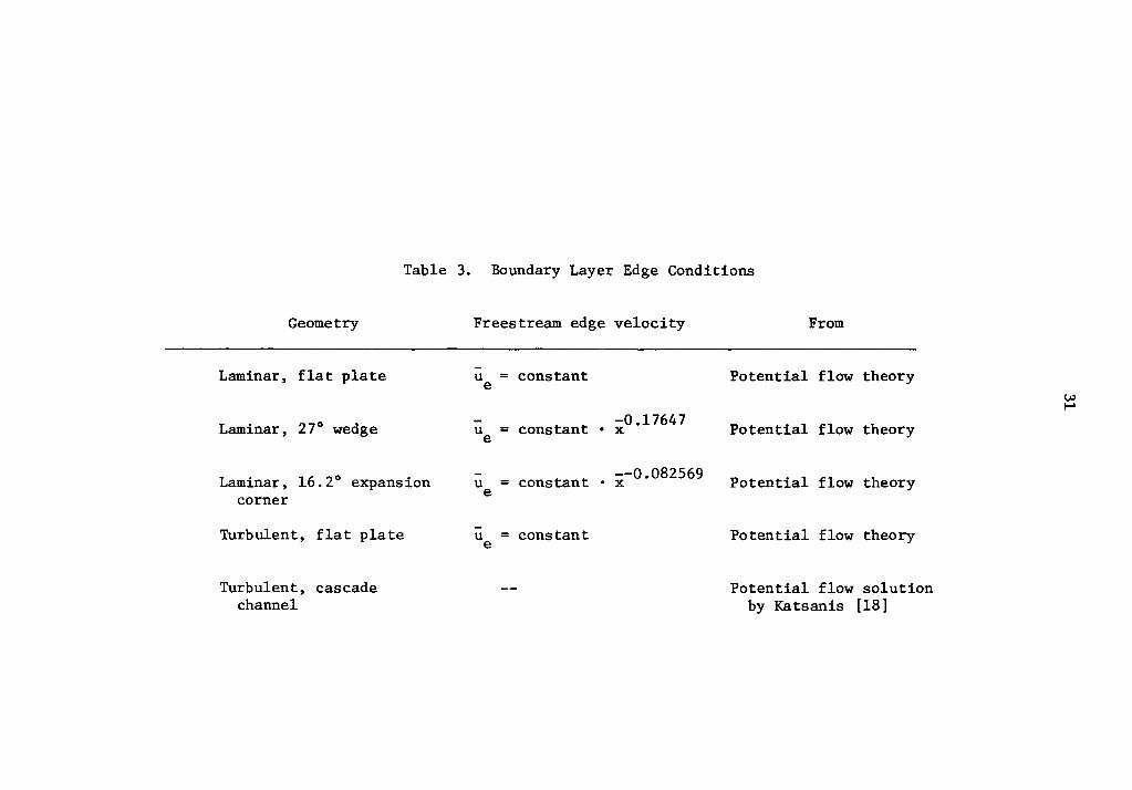
Table 3. Boundary Layer Edge Conditions
Geometry Freestream edge velocity From
Laminar, flat plate u = constant Potential flow theory e
Laminar, 27° wedge - -0.17647 Potential flow theory u = constant • x e
Laminar, 16.2° expansion - --0.082569 Potential flow theory u = constant • x e corner
Turbulent, flat plate u = constant Potential flow theory e
Turbulent, cascade -- Potential flow solution channel by Katsanis (18]
w I-'
32
The above condition in terms of the finite difference grid becomes
1 u - u m,n m,n-1 fly
< e: (3.34)
where the tolerance e: is given by the u profile at the initial
station. A mesh point is added and the solution at the mth station
repeated until the tolerance is met. The coarse nature of the grid
required to start several of the calculations necessitated the
specification of the edge tolerance by some means other than Eq. 3.34
applied to the initial velocity distribution. In these cases, the
edge tolerance was chosen sufficiently small so that the calculation
carried along several extra nodes essentially outside the boundary
layer.
3.4 The Coordinate Transformation
A coordinate transformation proves useful in allowing the solution
technique to "see" the high velocity gradient near the wall
characteristic of turbulent flow. Pierce [16] uses a simple technique
where the boundary layer thickness is represented by a geometric
series. Small steps are taken across the viscous sublayer with the
step size becoming increasingly larger across the turbulent core.
Pierce's method has the disadvantage of a complicated set of finite
difference equations. Cebeci [20] uses a combination Mangler-Levy-
Lees transformation stretching the boundary layer in both the x and

33
y directions. Cebeci's method results in a solution plane which has
a near constant boundary layer thickness with compressibility effects
greatly reduced. The coordinate transformation used here is
identical to that of Levine [7] which stretches the physical plane
near the wall. The finite difference solution to the equations is
conducted in the transformed plane with constant step sizes in both
the x and y direction. The stretching function is given by
y = G(y) tn [ (e-l)(t + a) + 1 J I l/N - (3.35)
where a and S are constants determined from the conditions on G(O)
and G'(O). The amount of stretching is controlled by the exponent
N. The first and second derivatives of the stretching function are
also required. Defining the intermediate quantity D,
D - (e-1) (~ + a) + 1 Qi
G' and G" may be written:
The inverse stretching function is given by
(3. 36)
(3.37)
(3.38)
34
(3.39)
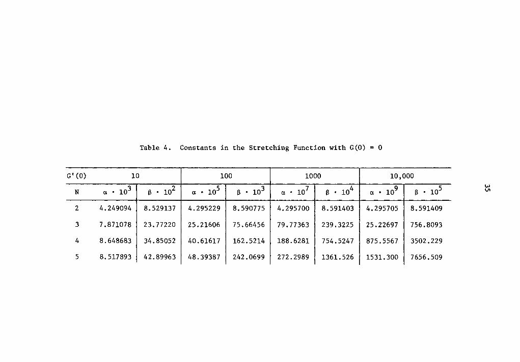
Values of~ and 8 for various G'(O) with G(O) = 0 are presented in
Table 4.
The coordinate transformation is applied only to turbulent
flow calculations. Numerical difficulties arose when stretching the
y coordinate in laminar flow as a result of the extremely small
velocities near the wall. The equations for laminar flow are
simplified by substituting:
y = G(y) = y
G' (y) = 1
G" (Y) 0 •
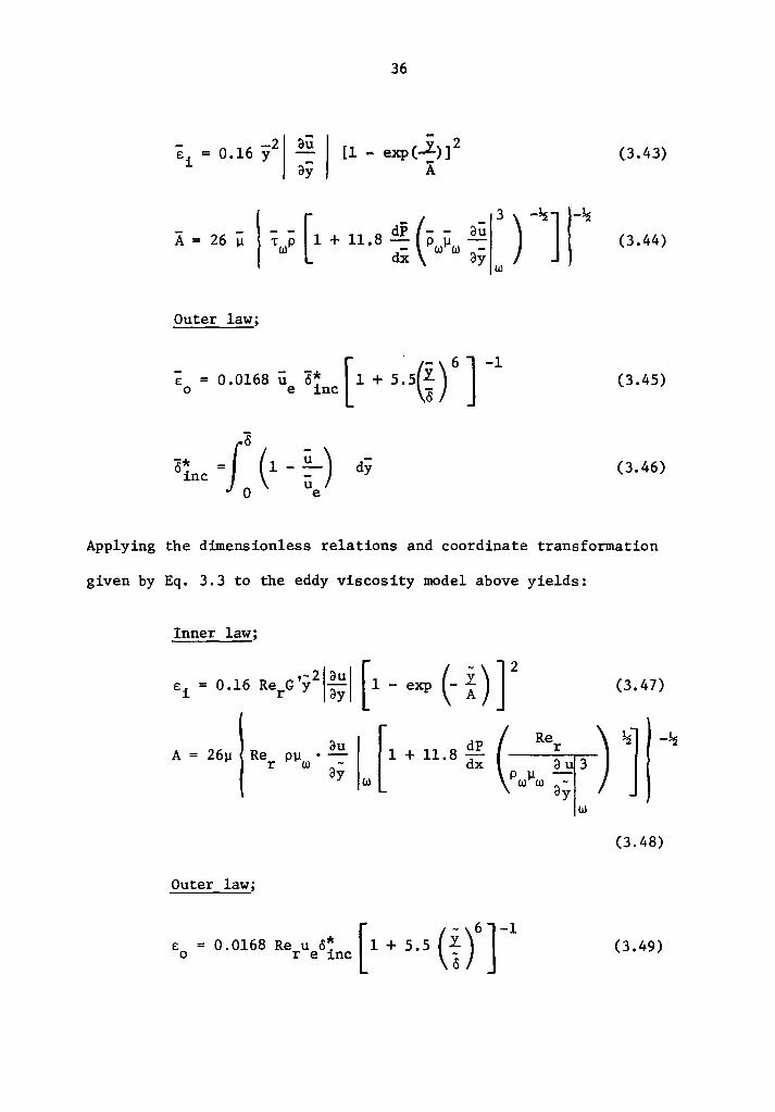
3.5 The Eddy Viscosity Model
(3.40)
(3.41)
(3.42)
The eddy viscosity concept is used to replace the Reynolds shear
stress in the time averaged momentum equation. A two-layer eddy
viscosity model developed by Cebeci [20] is incorporated into the
calculation technique. Cebeci's turbulent viscosity model consists
of the van Driest inner law and Clauser outer law, modified to
include the effects of compressibility, pressure gradient, and mass
injection normal to the wall. Cebeci's model as given below is in
simplified form neglecting mass injection normal to the wall.
Inner law;
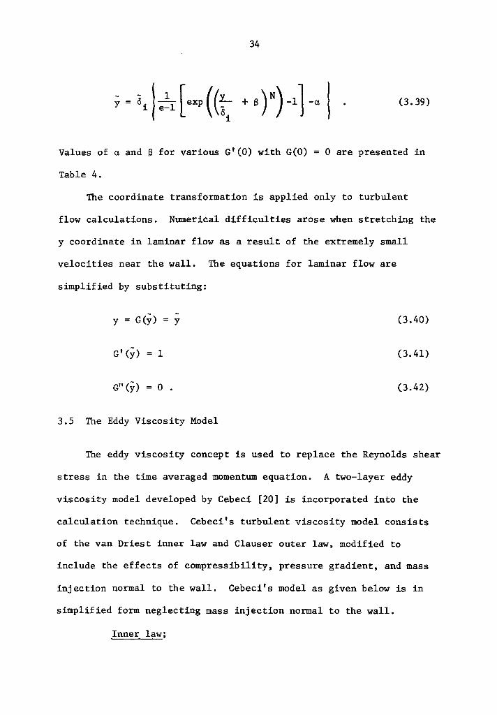
G' (0) 10
N (l • 10 3
2 4.249094
3 7 .871078
4 8.648683
5 8.517893
Table 4. Constants in the Stretching Function with G(O) = 0
100 1000 10,000
B • 102 (l • 10 5 B • 103
(l • 10 7 B • 104 (l • 10 9 B • 105
8. 529137 4.295229 8.590775 4.295700 8.591403 4.295705 8.591409
23. 77220 25.21606 75.66456 79. 77363 239.3225 25.22697 756.8093
34.85052 40.61617 162.5214 188.6281 754.5247 875.5567 3502.229
42. 89963 48.39387 242.0699 272. 2989 1361.526 1531. 300 7656.509
w \JI
36
- -2 Ei = 0.16 y (3.43)
A= 26 ii l --[ dP (- - au 3
T p 1 + 11. 8 - p µ -w - w w -dx ay w
(3.44)
Outer law;
c0 - 0.0168 u. <l~nc [ 1 + s.s~) 6 ] -l (3.45)
(3.46)
Applying the dimensionless relations and coordinate transformation
given by Eq. 3.3 to the eddy viscosity model above yields:
Inner law;
(3.47)
A = 26µ Jl + 11.8 !! (
Re r )1 w
(3.48)
Outer law;
e = 0.0168 Re u a*i (1 + 5.5 (i)6]-l o re~ ~
(3.49)
37
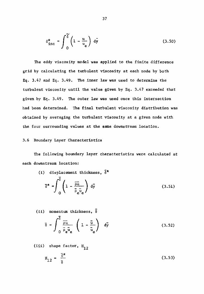
(3.50)
The eddy viscosity model was applied to the finite difference
grid by calculating the turbulent viscosity at each node by both
Eq. 3.47 and Eq. 3.49. The inner law was used to determine the
turbulent viscosity until the value given by Eq. 3.47 exceeded that
given by Eq. 3.49. The outer law was used once this intersection
had been determined. The final turbulent viscosity distribution was
obtained by averaging the turbulent viscosity at a given node with
the four surrounding values at the same downstream location.
3.6 Boundary Layer Characteristics
The following boundary layer characteristics were calculated at
each downstream location:
(i) displacement thickness, ~*
5* =Jo (1 - ~\i ti ) dy 0 Pe e
(3.51)
(ii) momenttllll thickness, e
(3.52)
(iii) shape factor, H12
8* (3. 53)

38
(iv) skin friction coefficient, Cf
(3. 54)
The integrations above were performed using the trapezoidal method
in the dimensionless plane. The wall shear stress for a Newtonian
fluid is given by
au. ay (3.55)
w
The velocity gradient in the y direction evaluated at the wall was
calculated using a technique suggested by Clausing [15]. Clausing
approximates the gradient at the wall with the arithmetic average of
a linear approximation and a parabolic approximation given by
aul ay w
1 ( 3 17 41 = l!.y 16 um,4 - 16 um,3 + 16 um,2 27 )
16 um,l
(3. 56)
The above finite difference relation is written for discrete points
in the dimensionless, stretched plane. Applying the no-slip condition
at the wall, the velocity gradient in the physical plane may be written
aii ay w
= urG I (0) ( 1- u E 16 m,4
r
17 41 ) --u +-u 16 m,3 16 m,2
(3.57)
Clausing's technique for evaluating derivatives at the wall was used
in both the determination of the skin friction coefficient and the
39
evaluation of the eddy viscosity model, Eq. 3,48.
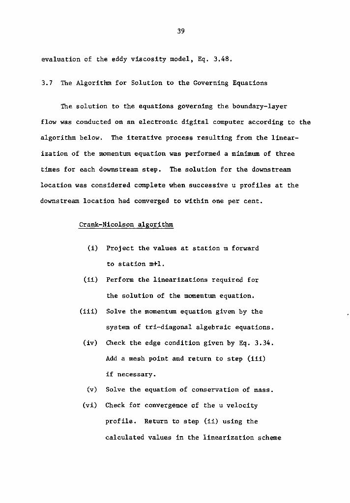
3.7 The Algoritlun for Solution to the Governing Equations
The solution to the equations governing the boundary-layer
flow was conducted on an electronic digital computer according to the
algorithm below. The iterative process resulting from the linear-
ization of the momentum equation was performed a minimum of three
times for each downstream step. The solution for the downstream
location was considered complete when successive u profiles at the
downstream location had converged to within one per cent.
Crank-Nicolson algorithm
(i) Project the values at station m forward
to station m+l.
(ii) Perform the linearizations required for
the solution of the momentum equation.
(iii) Solve the moment1.m1. equation given by the
system of tri-diagonal algebraic equations.
(iv) Check the edge condition given by Eq. 3.34.
Add a mesh point and return to step (iii)
if necessary.
(v) Solve the equation of conservation of mass.
(vi) Check for convergence of the u velocity
profile. Return to step (ii) using the
calculated values in the linearization scheme
40
if necessary.
(vii) Finalize the step downstream by
calculating the boundary layer characteristics.
The code exists in two forms, one for laminar boundary layer
calculations and a second for the turbulent counterpart. No capability
exists in either code for transition from laminar to turbulent flow.
The codes are constructed using functional blocks, or subroutines,
to carry out the algorithm. The Appendix contains a flow diagram
showing calls to and operations performed by the various functional
blocks. The use of functional blocks should enable a later user
to investigate the feasibility of other stretching functions, eddy
viscosity models, etc •. Major differences between the laminar and
turbulent codes exist in the subroutines controlling the stretching
function, the eddy viscosity model, and the initial velocity profiles.
For the laminar case, the stretching function is replaced by Eq. 3.40-
Eq. 3.42, the eddy viscosity is "turned off" with £ = 0, and the
initial velocity profiles are given by Eq. 3.24 and Eq. 3.25. Both
codes contain temperature dependent fluid properties in array form
so that compressibility effects may be incorporated into the analysis.
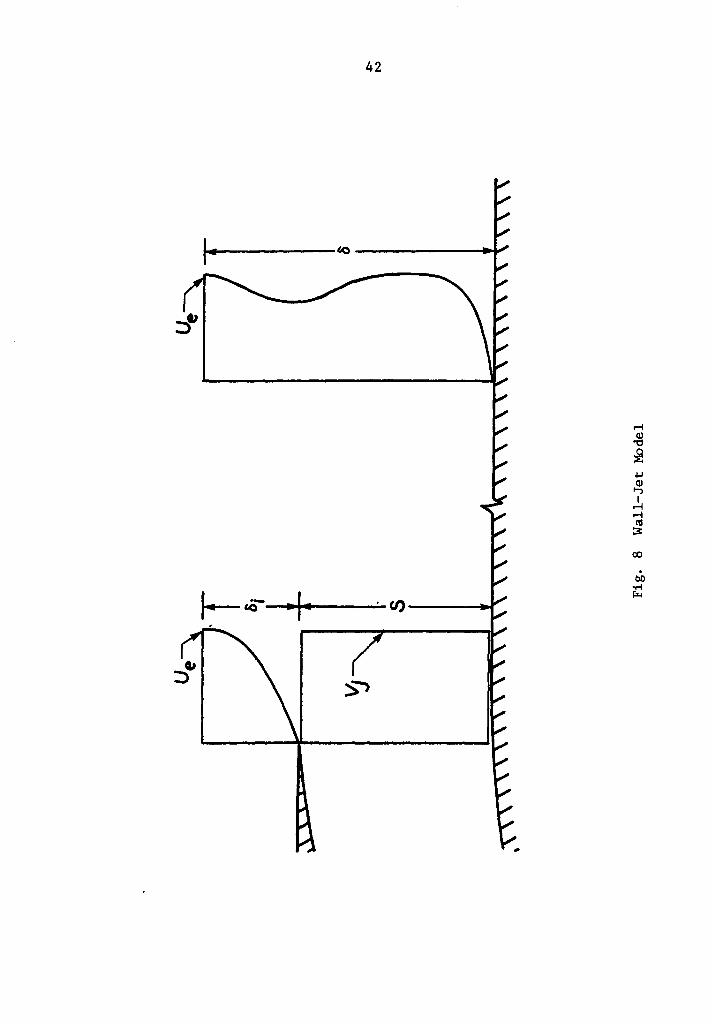
3.8 The Wall-Jet Model
The assumed form of the injected velocity profiles consists of
some initial boundary layer development standing over a block or slug
flow approximation for the flow issuing from the wall jet. The
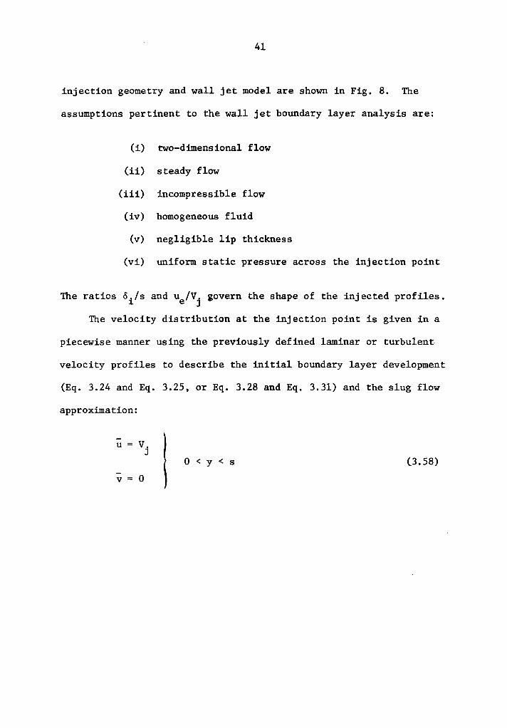
41
injection geometry and wall jet model are shown in Fig. 8. The
assumptions pertinent to the wall jet boundary layer analysis are:
(i) two-dimensional flow
(ii) steady flow
(iii) incompressible flow
(iv) homogeneous fluid
(v) negligible lip thickness
(vi) uniform static pressure across the injection point
The ratios oi/s and u /V. govern the shape of the injected profiles. e J
The velocity distribution at the injection point is given in a
piecewise manner using the previously defined laminar or turbulent
velocity profiles to describe the initial boundary layer development
(Eq. 3.24 and Eq. 3.25, or Eq. 3.28 and Eq. 3.31) and the slug flow
approximation:
u = V. J
0 < y < s (3.58) v = 0
42
00
,._ c<,--.... ~lr-i~t----__,.;·:.. Cl'J----..r
4. Results
Several boundary layer flows were investigated to test the
validity of the Crank-Nicolson algorithm as employed in the
investigation. Three laminar boundary layer flows subjected to
various pressure gradients along with turbulent, zero pressure
gradient flow were considered. The boundary layer flow over the
airfoil section was then calculated and compared with a second
solution technique. Finally, the boundary layer flow with wall jet
injection was calculated. The interaction of the wall jet with the
initial boundary layer for zero pressure gradient flow and the flow
over the airfoil section was considered.
4.1 Laminar Boundary Layer Calculations
Laminar boundary layer calculations were performed for the flow
over three geometries: a flat plate with zero pressure gradient, a
27° half-angle wedge with negative (favorable) pressure gradient, and
a 16.2° expansion corner with positive (adverse) pressure gradient.
These three cases were investigated to test the response of the pro-
cedure to various pressure gradients. The solutions to the boundary
layer flow over these geometries are well known and members of a
large family of solutions known as the Falkner-Skan wedge flows. The
Falkner-Skan solutions are similarity solutions where
_ [m+l ue J n=y --·-2 --vx
43
(4.1)
f I (n) u =-
u e
44
(4. 2)
and m is a parameter controlling the pressure gradient -- identical
to the quantity m in Eq. 3.32. Substituting Eq. 4.1 and Eq. 4.2
-into Eq. 3.2 with £ = 0 there results
subject to
d3f 2 +f·u
dn 3 dn 2
the boundary
f(O) = df (0) dn
df (co) = 1 dn
+ : 1 11 +(:~r l
conditions
= 0
= 0 (4.3)
(4.4)
(4.5)
The solution to Eq. 4.3 may be changed to an initial value 2 2 problem if the value of d f/dn (@ n=O) can be selected to satisfy
the asymptotic condition Eq. 4.5. White [21] has solved Eq. 4.3 and
lists values of d2f/dn 2 (@ n=O) which satisfy the asymptotic condition
for various values of the parameter m. For the three geometries above:
(i) flat plate; d2f/dn 2(@ n=O) = 0.46960
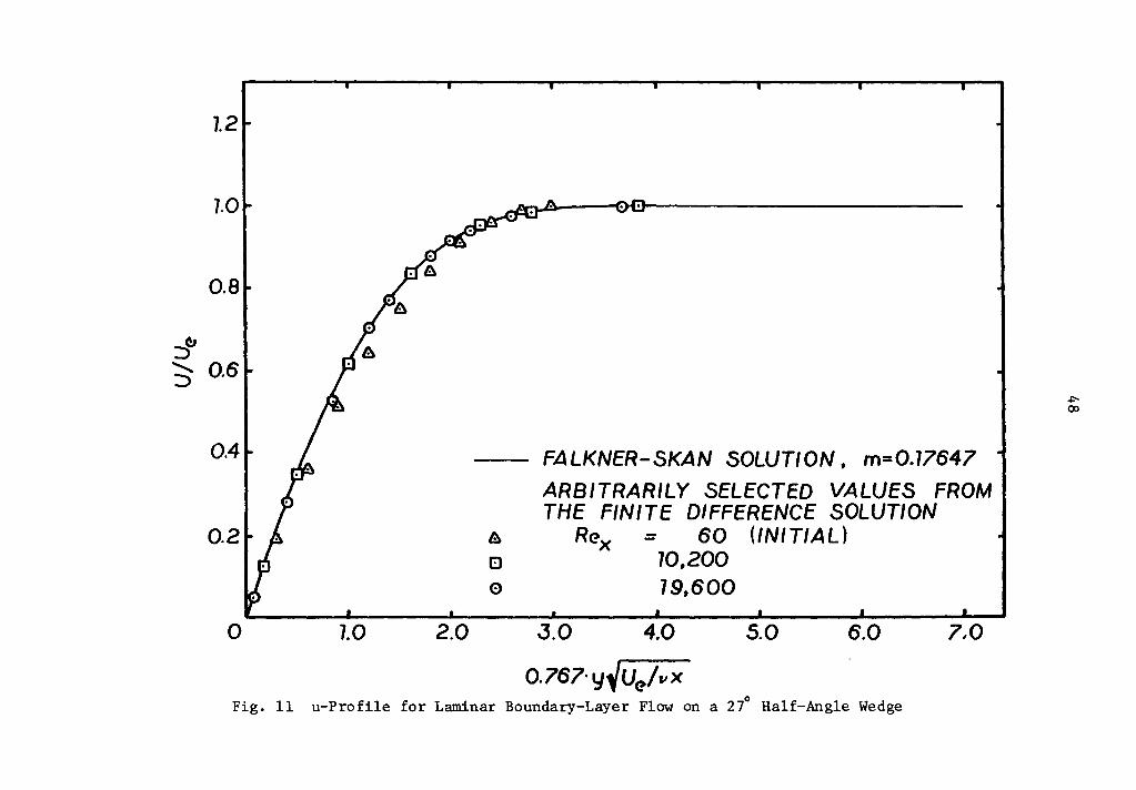
(ii) 2 2 27° half-angle wedge; d f/dn (@ n=O) = 0.77476
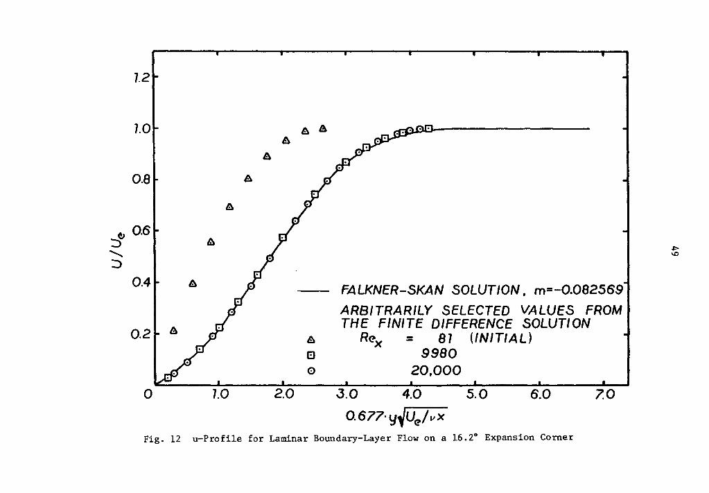
(iii) 2 2 16.2° expansion corner; d f/dn (@ n=O) = 0.12864
Equation 4.3 was integrated numerically using IBM's Continuous
System Modeling Program (CSMP) with the values for the initial
conditions above. The boundary layer parameters given by Eq. 3.51-
Eq. 3.54 were included in the CSMP calculation. The resulting
boundary layer characteristics are:
(i) flat plate;
e 0.664 - = x ~ x
Hl2 = 2.59
cf 0.664 = ~ x
(ii) 27° half-angle wedge;
e - = x
0.503 ~ x
= 2.37
1.19 cf=--lie x
(iii) 16.2° expansion corner
e - = x 0.838 ~ x
= 3.29
0.174 ~ x
45
(4 .6)
(4. 7)
(4.8)
(4. 9)
(4 .10)
(4.11)
(4.12)
(4.13)
(4.14)
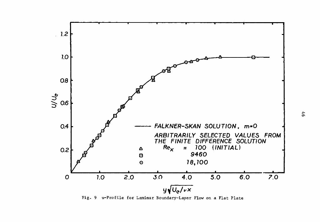
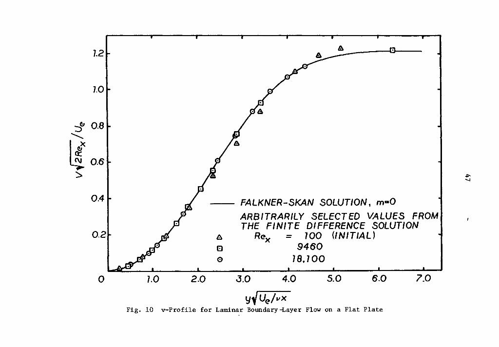
The results from the Crank-Nicolson algorithm for the three
geometries are shown in Fig. 9 - Fig. 15. The predictions from the
Crank-Nicolson algorithm agree well with the Falkner-Skan similarity
1.2
1.0
O.B
::t ~ 0.6
0.4
0.2
0 1.0 2.0
-- FALKNER-SKAN SOLUTION, m=O ARBITRARILY SELECTED VALUES FROM THE FINITE DIFFERENCE SOLUTION
/;)
8 0
J.O
Rex = 100 (INITIAL) 9460
1B,100
4.0 5.0 6.0 7.0
y'Ue/vx Fig. 9 u-Profile for Laminar Boundary-Layer Flow on a Flat Plate
.p.
°'
1.2
1.0
~ 0.8
' I ~x ~ 0.6
:>
0.4
0.2
0 1.0 2.0
&
FALKNER-SKAN SOLUTION, m•O ARBITRARILY SELECTED VALUES FROM THE FINITE DIFFERENCE SOLUTION
& Rex = 100 (I NIT/AL) EJ 9460 0 18,100
J.O 4.0 5.0 6.0 7.0
y~Ue/11x Fig. 10 v-Profile for Laminar Boundary-Layer Flow on a Flat Plate
~ -...J
1.2
1.0
0.8
::>~ :>- 0.6
0.4
0.2
0
Fig. 11
1.0 2.0
&.
8 0
FALKNER-SKAN SOLUTION, m=0.17647 ARBITRARILY SELECTED VALUES FROM THE FINITE DIFFERENCE SOLUTION
Rex = 60 (INITIAL) 10,200 19,600
J.O 4.0 5.0 6.0 7,0
0.767· y~Ue/vx 0 u-Profile for Laminar Boundary-Layer Flow on a 27 Half-Angle Wedge
.i:-00
7.2
7.01- Ill ~ e.
Ill
0.8 e.
Ill
~ 0.6 ~ I &
./ I .po I.Cl
:::> 0.4t- Ill ir.11 FALKNER-SKAN SOLUTION, m=-0.082569
El 0
; ARBITRARILY SELECTED VALUES FROM
0.21- A cl' THE FINITE DIFFERENCE SOLUTION Ill Rex : 81 (INITIAL) 8 9980 0 20,000
0 7.0 2.0 J.O 4.0 5.0 6.0 7.0
0.677·y~Ue/vx Fig. 12 u-Profile for Laminar Boundary-Layer Flow on a 16.2° Expansion Corner
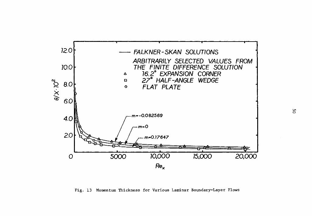
0 5000 70,000 Rex
75,000 20,000
Fig. 13 Momentum Thickness for Various Laminar Boundary-Layer Flows
72.0t - FALKNER-SKAN SOLUTIONS ARBITRARILY SELECTED VALUES FROM
70.08 THE FINITE DIFFERENCE SOLUTION A 16.2° EXPANSION CORNER l:J 27° HALF-ANGLE WEDGE
a.01 a FLAT PLATE "' 0 ,.._ ()- 6.0
I\ \ 4.o·· -
I \ "
2.0~~~
0 5000
m•0.17647 I
m•O
I I r- m·-0.082569
10,000 Rex
75.000 20,000
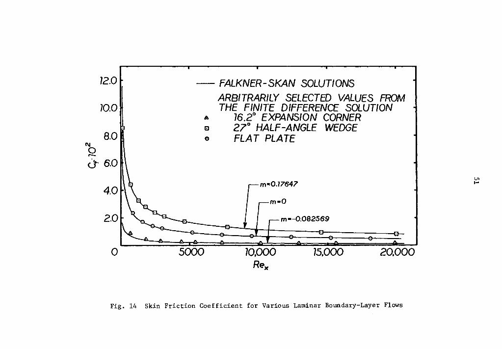
Fig. 14 Skin Friction Coefficient for Various Laminar Boundary-Layer Flows
I V"I ......
4.0 .. -. . -.---
-- FALKNER-SKAN SOLUTIONS ARBITRARILY SELECTED VALUES FROM THE FINITE DIFFERENCE SOLUTION
s,, 16.2° EXPANSION CORNER e 27° HALF ANGLE WEDGE 0 FLAT PLATE
A 6 6 ei A G B Ca l
& &;. &;. . m=-0.082569 C\I :t:"" J.O 1o
~ o r:m•O 0.-----~ 0,------' o----
b - -~ ~ .:.
lm=0.::647 ~
2.01o J-
. . - -
.
0 5000 70,000 Rex
75,000 20,000
Fig. 15 Shape Factor for Various Laminar Boundary-Layer Flows
V1 N
53
solutions. Differences as high as 10 per cent between the calcul-
ated skin friction coefficient and the value given by the similarity
solution were noted for the expansion corner calculation. The
discrepancy can be attributed to the step-size in the downstream
direction. The Crank-Nicolson algorithm was observed to be quite
sensitive to the downstream step-size for the adverse pressure
gradient calculation. The laminar calculations were conducted
using downstream steps on the order of the initial boundary layer
thickness for the zero and favorable pressure gradient calculations
and a step of approximately one-fourth of the initial boundary
layer thickness for the adverse pressure gradient flow. Figure
15 gives some indication of the downstream distance required for the
calculation to relax from the asswned initial boundary layer thick-
ness and velocity distributions to the proper solution. The finite
difference solution relaxes to the similarity solution rapidly for
the zero and favorable pressure gradient flows. The relaxation
distance is much greater for the adverse pressure gradient flow.
As shown by the range of Reynolds numbers in Fig. 9 - Fig. 12,
all calculations were begun near the leading edge (for the flat
plate) or the vertex (for the wedge and expansion corner) of the
geometries. Pressure gradients are severe in these regions. Thus
it is believed that these flows are stringent tests of the calculation
procedure. The algorithm was also applied to the flow into the
leading edge of a flat plate to check the ability of the calculation
procedure to reduce a block, or slug profile to the similarity
54
solution. The algorithm performed adequately in this case.
4.2 Turbulent Boundary Layer Calculations
Turbulent boundary layer flow on a flat plate and on both
surfaces of the cambered NACA 0012 airfoil section was considered.
The results from the Crank-Nicolson finite difference algorithm are
compared with the two-parameter integral analysis of Moses [17].
Tne turbulent boundary layer calculations on the cambered
NACA 0012 airfoil section were performed for ideal conditions in
the TRL cascade facility. The facility has incorporated a centrifugal
blower powered by a 1.49 kw motor. It is assumed that the motor power
capacity is delivered to the air flowing through the cascade with no
increase in static pressure or temperature. Thus, the motor power
is converted to the kinetic energy of the air entering the cascade
tunnel. 2 The tunnel cross section has an area of 0.0265 m • The
cambered NACA 0012 airfoil was constructed with a blade span of
0.102 m and pitch of 0.117 m. A simple energy balance applied to the
cascade air delivery equipment yields a mean velocity entering the
cascade blade channel of 46.6 m/sec and a mass flow per blade
channel of 0.619 kg/sec. Ambient conditions were assumed to be 4 27 C and 9.63•10 Pa.
The idealized cascade conditions were used in the potential flow
solution of Katsanis [18] to determine the pressure gradient driving
the boundary layer flow. Figure 16 shows the input data for the
potential flow code. The results of the potential flow solution are
SUHSONIC BLADE-TO-BLADE INVISCID FLOW PROGRAM PROGRAM TSONIC
WESKAT Ill.TA SET FOR NACA0012 CASCADE BLADES IALPHAl=O.O,ALPHAE=60.0,P=O.ll7ll
GAM AR TIP o.150000E 01 o.1oooooe 04 o.1oooooe 01
8ETAI BETAO CHOROF O.O -0.534800E 02 0.1079t>OE 00
R EDFAC DENTOL CUTOFF o.1oooooe 01 o.100000E-01 o.eoooooe oo
MBI MBO MM NBBI NBL NRSP 11 41 0 0 51 30 30 2
BLADE SURFACE 1 -- UPPER SURFACE Rll ROl BETil
0.176t>OOE-02 O.BB3000E-03 0.550000E 02 MSPl ARRAY
o.100000E 01 o.200600E-02 o.39t>600E-02 0.4t>l920E-Ol 0.5857t>OE-Ol 0.6927001:-01 o.100000E 01
ntSPl ARRAY o.100000E 01 o.493oooe-02 o.6t>6900E-02
-0.116150t:--Ol -0.292240E-Ol -0.4Yl850E-Ol o.100000E 01
BLADE SURFACE 2 LOWER SURFACE RI2
0.176600E-02 MSP2 ARRAY
o.1oooooe 01 0.363540E-Ol o. toooooE o
THSP2 ARRAY
ROZ BETI2 0.883000E-03 -0.435000E 02 0.183300E-02 0.350000E-02 0.474310E-Ol 0.580670E-01
o.1oooooe 01 -o.5o37ooe-oz -o.1014ooe-02 -0.378t>5gE-01 -0.523810E-Ol -0.685630E-Ol 0.10000 E 01
MR ARRAY -o.1oooooe 01 o.100000E 01
RMSP ARRAY 0.559100E 00 0.559lOOE 00
BESP ARRAY 0.101600E 00 0.101600E 00
RHOIP o.111eooE 01
STGRF -O.l62640E 00
BETOl -0.625000E 02
0.798000E-02 Oo786270E-Ol
0.850600E-02 -Oo 7069YOE-O l
BET02 -0.510000E 02
0.673800E-02 o. 683309E-O l
-o.1ooeooE-ol -0.861300E-O
WTFL 0.619100E 00
SPLNOl O. l?OOOOE 02 O. U3690E-Ol 0.869740E-Ol
0.935000E-Ol -0.934460E-Ol
SPLND2 o.nooooE 02 Oo932100E-02 0. 783240E-Ol
-O. l24590E-01 -o. 04911E 00
o.o
O.l62020E-Ol 0.943789£:-01
0.889500E-02 -O.ll68110E 00
0.130190E-01 0.879800E-Ol
-O.l50960E-01 -o. 24610E 00
BLOAT AANDK ERSOR STRFN SLCRD INTVL SURVL ICONT NLAST JFLOW JOUT JGRAPH 1 0 0 0 0 0 1 1 1 1 1 l
OMEGA o.o
0.2425901:-01 O.lOOY81E 00
0.646700E-02 -0 .1401144E 00
O.l90400E-Ol 0.973660E-Ol
-0 .200820E-Ol -0.144866E 00
ORF o.o
0.320200t-Ol 0.104036£: 00
O. l93500E-02 -0.153038E 00
0.24Y300E-Ol 0.10l996E 00
-0 • 25 48 lOE-0 l -O.l5!it218E 00
Fig. 16 Input to the Potential Flow Solution in the Cascade Blade Channel
V1 V1
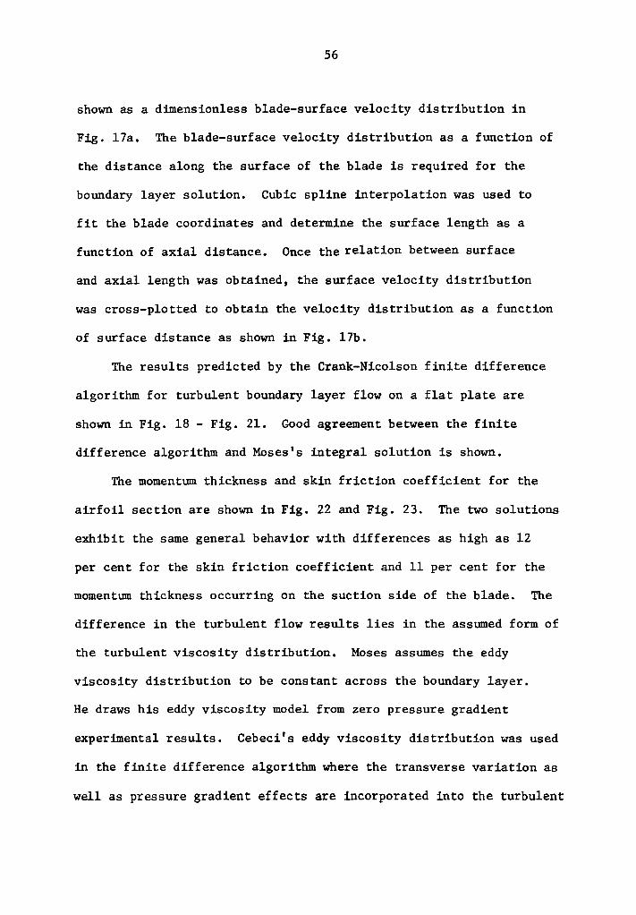
56
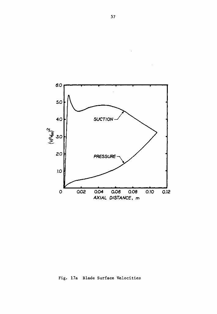
shown as a dimensionless blade-surface velocity distribution in
Fig. 17a. The blade-surface velocity distribution as a function of
the distance along the surface of the blade is required for the
boundary layer solution. Cubic spline interpolation was used to
fit the blade coordinates and determine the surface length as a
function of axial distance. Once the relation between surface
and axial length was obtained, the surface velocity distribution
was cross-plotted to obtain the velocity distribution as a function
of surface distance as shown in Fig. 17b.
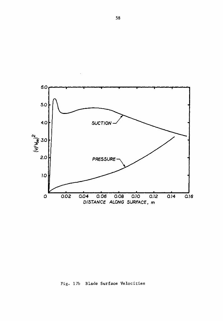
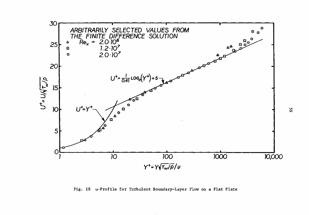
The results predicted by the Crank-Nicolson finite difference
algorithm for turbulent boundary layer flow on a flat plate are
shown in Fig. 18 - Fig. 21. Good agreement between the finite
difference algorithm and Moses's integral solution is shown.
The momentum thickness and skin friction coefficient for the
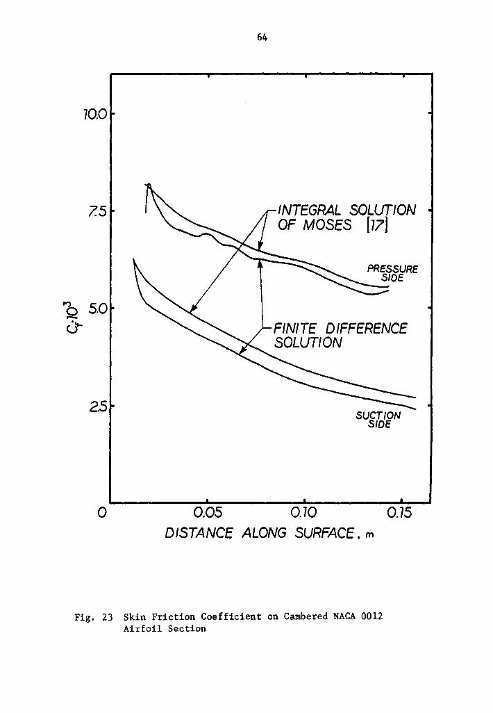
airfoil section are shown in Fig. 22 and Fig. 23. The two solutions
exhibit the same general behavior with differences as high as 12
per cent for the skin friction coefficient and 11 per cent for the
momentmn thickness occurring on the suction side of the blade. The
difference in the turbulent flow results lies in the assmned form of
the turbulent viscosity distribution. Moses assumes the eddy
viscosity distribution to be constant across the boundary layer.
He draws his eddy viscosity model from zero pressure gradient
experimental results. Cebeci's eddy viscosity distribution was used
in the finite difference algorithm where the transverse variation as
well as pressure gradient effects are incorporated into the turbulent
57
5.0
4.0
~ .J J.O ~ -
2.0
7.0
o 0.02 o.04 006 a oe 0.70 0.72 AXIAL DISTANCE, m
Fig. 17a Blade Surface Velocities
58
5.0
4.0
(\J
'J3.0 ~ -
2.0
1.0
0 0.02 0.04 0.06 0.08 0.10 0.12 0.14 076 DISTANCE ALONG SURFACE, m
Fig. 17b Blade Surface Velocities
JOr~:-_-::--:--~.-~~~~.--~~~~.-~~~---
ARBITRARILY SELECTED VALUES FROM e a e
25
20
I~ ~ 15 ~ II
-s 10
5
THE FINITE DIFFERENCE SOLUTION ~ Rex = 2.0·106
8 1.2·107
e 2.0·107
U+= O.~l LOG~y+)+s
A 8
10
a e
8
100
y+= Y~TwlP/v 7000
Fig. 18 u-Profile for Turbulent Boundary-Layer Flow on a Flat Plate
10.(XXJ
VI \0
'b ,.._ . )( ~
3.0.-------..----~----~------
2.0
1.0
0
FINITE DIFFERENCE SOLUTION
INTEGRAL SOLUTION OF MOSES [77]
0.5·KY 1.0·107 Rex
7.5·71 2.0·10
Fig. 19 Momentum Thickness for Turbulent Boundary-layer Flow on a Flat Plate
0\ 0
4.0r----~------..----....------
J.Ot !FINITE DIFFERENCE SOLUTION
' 'b ,._ ·c.-u
I I
INTEGRAL SOLUTION 2.0~ OF MOSES [77] , °' ......
0 0.5·KY 7.0·KY 7.5· 107 2.0·107
RE'x
Fig. 20 Skin Friction Coefficient for Turbulent Boundary-Layer Flow on a Flat Plate
C\I -:r:
2.0r-----r-------,..------....,------
J.5L
I
1.0~
0
1FINITE DIFFERENCE SOLUTION
l,NTEGRAL SOLUTION OF MOSES [77]
0.5·707 1.0·107
Rex 1.5·107
...
2.0·707
Fig. 21 Shape Factor for Turbulent Boundary-Layer Flow on a Flat Plate
0\ N
5.0
4.0
e ~. J.0 0 ,...... .
2.0
7.0
0
63
INTEGRAL SOLUTION OF MOSES [77]
0.05
SUCTION SIDE
FINITE DIFFERENCE SOLUTION
0.70
PRESSURE SIDE
0.75 DISTANCE ALONG SURFACE, m
Fig. 22 Momentum Thickness on Cambered NACA 0012 Airfoil Section
70.0
7.5
'b 5.0 ,..._ .!t-u
2.5
0
64
0.05
INTEGRAL SOLUTION OF MOSES (77)
PRESSURE SIDE
FINITE DIFFERENCE SOLUTION
0.70
SUCTION SIDE
0.75 DISTANCE ALONG SURFACE, m
Fig. 23 Skin Friction Coefficient on Cambered NACA 0012 Airfoil Section
65
viscosity model. The good agreement for zero pressure gradient flow
between the two calculations follows from the nature of Moses's
eddy viscosity model.
The turbulent boundary layer calculations on the blade surfaces
were started at locations corresponding to 10 per cent of the camber
line length. The flat-plate approximation for the initial boundary -4 4 layer development yielded thicknesses of 4.50•10 m and 8.10•10- m
for the suction and pressure sides respectively.
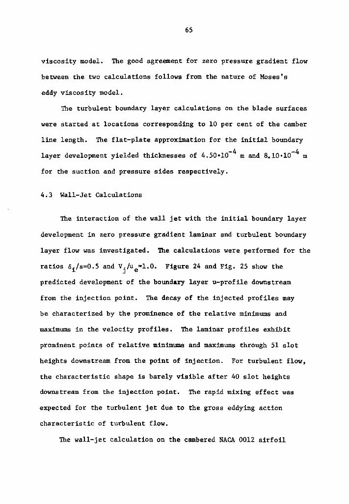
4.3 Wall-Jet Calculations
The interaction of the wall jet with the initial boundary layer
development in zero pressure gradient laminar and turbulent boundary
layer flow was investigated. The calculations were performed for the
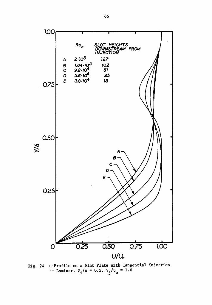
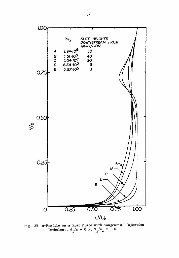
ratios oi/s=0.5 and V./u =l.O. Figure 24 and Fig. 25 show the J e predicted development of the boundary layer u-profile downstream
from the injection point. The decay of the injected profiles may
be characterized by the prominence of the relative minimums and
maximums in the velocity profiles. The laminar profiles exhibit
prominent points of relative minimums and maxi.mums through 51 slot
heights downstream from the point of injection. For turbulent flow,
the characteristic shape is barely visible after 40 slot heights
downstream from the injection point. The rapid mixing effect was
expected for the turbulent jet due to the gross eddying action
characteristic of turbulent flow.
The wall-jet calculation on the cambered NACA 0012 airfoil
66
100r-----------------------------
Q75
0.50
025
0
A a c D E
z.705 1.64·105 9.2·7o4 5.6·7a4 J.8·1a4
0.25
SLOT HEIGHTS DOWNSTREAM FROM IN'1ECTION
127 102 51 25 73
0.50 0.75 U/(k
7.00
Fig. 24 u-Profile on a Flat Plate with Tangential Injection -- Laminar, oi/s = 0.5, Vj/ue = 1.0
1.00
R~x
A 7.84·706 a 1.57 ·106 c 1.04·706 0 6.J4·7os
075 E 5.67·7o5
0.50
0.25
0 0.25
67
SLOT HEIGHTS DOWNSTREAM FROM INJECTION
50 40 20 s J
0.50 U/U~
0.75 7.00
Fig. 25 u-Profile on a Flat Plate with Tangential Injection -- Turbulent, o./s = 0.5, V./u = 1.0
1 J e
68
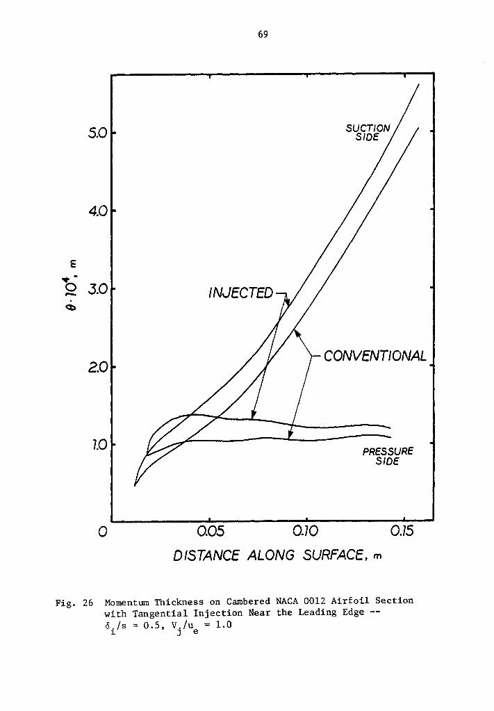
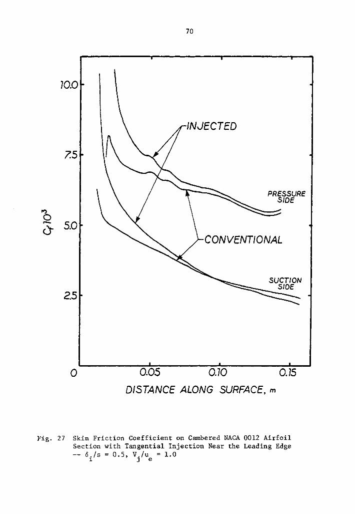
section was begun at 10 per cent of the camber line length. Again,
the wall jet was constructed with the ratios oi/s=0.5 and Vj/ue=l.O.
Figure 26 and Fig. 27 show the momenttun thickness and skin friction
coefficient for the injected boundary layer on the blade section. A
large increase in the skin friction for the injected boundary layer
with respect to the conventional case occurs. The skin friction
coefficient for the injected boundary layer is most certainly affected
by the wall-jet model where a high velocity gradient near the wall
results from the slug flow approximation. A more realistic model
for the flow issuing from the wall jet would be the velocity profile
resulting from an analysis of the turbulent flow between infinite
parallel plates. The momentmn thickness on the suction side of the
blade is shown to be approximately 3.5•10-5m greater than the non-
injected boundary layer. On the pressure side of the blade, the
momentum thickness shows a rapid increase over the non-injected
boundary layer within 14 slot heights downstream from the point of
injection--declining from this point owing to the favorable pressure
gradient along the pressure side of the blade. The momentum thickness
at the trailing edge of the blade for the injected boundary layer is
10 per cent and 11 per cent greater than the non-injected boundary
layer for the suction and pressure sides respectively.
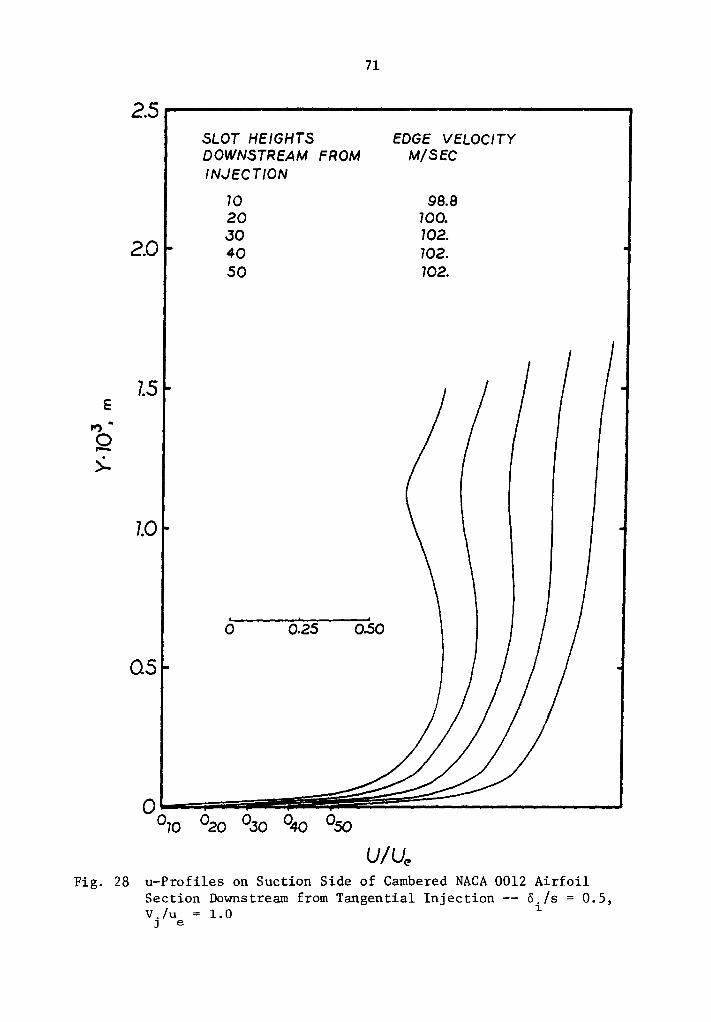
The u profiles on the blade section at several locations down-
stream from the point of injection are shown in Fig. 28 and Fig. 29.
The characteristic shape of the injected profiles persists through
30 slot heights downstream from the injection point on the suction
5.0
4.0
E ... 2 J.O . <:I)
2.0
7.0
0
69
0.05 0.70
CONVENTIONAL
PRESSURE SIDE
0.75 DISTANCE ALONG SURFACE, m
Fig. 26 Momentum Thickness on Cambered NACA 0012 Airfoil Section with Tangential Injection Near the Leading Edge --o. /s = 0.5, v./u = 1.0
1 J e
70.0
7.5
,_, 0 0- 5.0
2.5
0
70
0.05
PRESSURE SIDE
CONVENTIONAL
0.70 0.75 DISTANCE ALONG SURFACE, m
Fig. 27 Skin Friction Coefficient on Cambered NACA 0012 Airfoil Section with Tangential Injection Near the Leading Edge -- o./s = 0.5, V./u = 1.0
1 J e
E ,., . Q )..
71
2.5------------------
2.0
7.5
7.0
05
SLOT HEIGHTS DOWNSTREAM FROM INJECTION
70 20 JO 40 50
0 0.25
EDGE VELOCITY M/SEC
U/U<!
98.8 700. 702. 702. 702.
Fig. 28 u-Prof iles on Suction Side of Cambered NACA 0012 Airfoil Section Downstream from Tangential Injection -- o./s = 0.5, V. /u = 1.0 1
J e
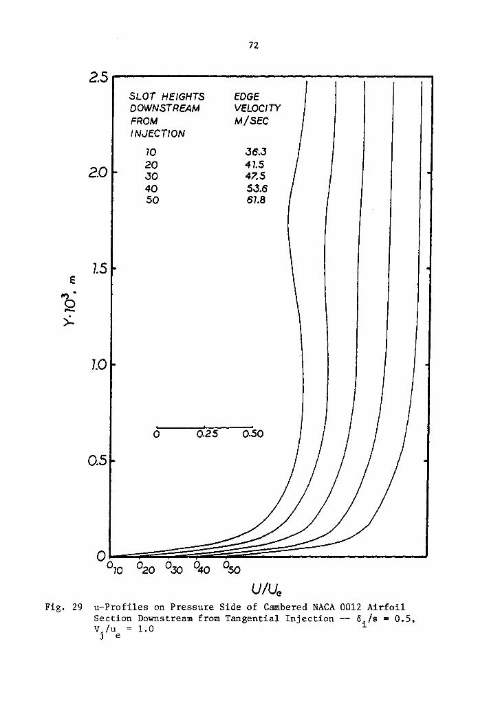
72
2.5 SLOT HEIGHTS EDGE DOWNSTREAM VELOCITY FROM M/SEC INJECTION
70 J6.J
2.0 20 41.5 JO 47.5 40 5J.6 50 61.8
7.5 E .., ..
0 ,.._
7.0
0
0.5
UIUe Fig. 29 u-Profiles on Pressure Side of Cambered NACA 0012 Airfoil
Section Downstream from Tangential Injection -- 5./s = 0.5, v./u = LO 1
J e
73
side of the blade versus 20 slot heights for the pressure side.
Tiie downstream step-size required for the prediction of the
injected boundary layer development was smaller than the downstream
step utilized in the conventional boundary layer calculations.
Downstream steps of 20 per cent and 1.7 per cent of the total
boundary layer thickness (including the slot height) at the initial
station were used in the wall-jet calculations with no pressure
gradient. Downstream steps of 0.24 per cent and 1 per cent of the
total boundary layer thickness at the point of injection were
necessary to predict the boundary layer flow on the pressure and
suction sides of the blade. In all cases investigated, the step-size
was determined by solving the governing equations using a step-size
equal to the initial boundary layer thickness. The downstream step
was repeatedly halved until two solutions, one with a step of 6x and
a second with a step of 6x/2, produced the same results.
5. Conclusions and Recommendations for Further Study
The Crank-Nicolson finite difference algorithm employed in
the solution to the boundary layer equations was found to perform
well when applied to conventional boundary layer flows. The
predicted results from the finite difference algorithm were found
to agree well with the Falkner-Skan similarity solutions for three
laminar boundary layer flows: flow into a 27° half-angle wedge,
flow on a flat plate, and flow around a 16.2° expansion corner.
The finite difference predictions were also found to agree well
with an integral solution for turbulent boundary layer flow on
a flat plate and on representative combustion turbine blade sur-
faces. The algorithm was found to be capable of predicting the
behavior of the boundary layer downstream from the tangential
injection of a second stream.
Further efforts to utilize the algorithm should be conducted
in the following areas.
(i) An eddy viscosity model applicable to the mixing of
some initial boundary layer development with the flow
issuing from a tangentially oriented wall jet should
be sought. It is recognized that the two-layer
model used in the solutions presented may not prove
to be an accurate description of the £ variation in
wall-jet flow. The hibh gradients at the wall near
the injection point resulting from the slug flow
approximation were found to switch the £ model to
74
75
the outer law prematurely.
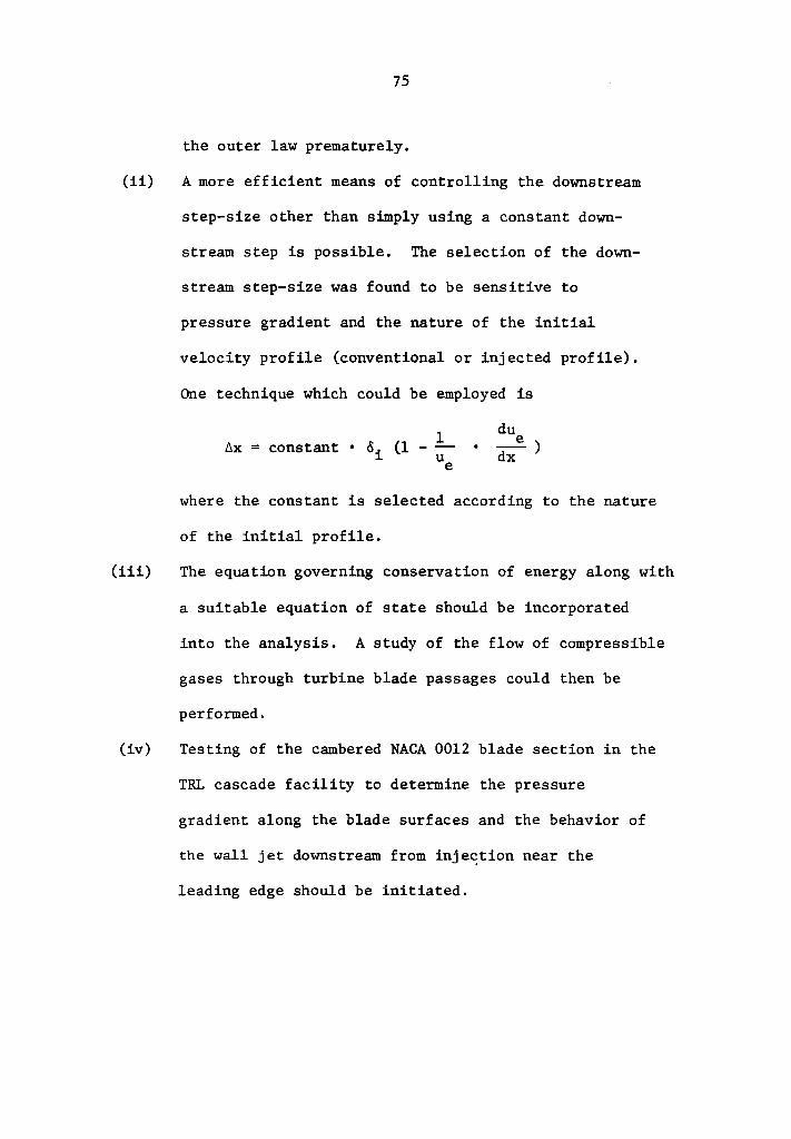
(ii) A more efficient means of controlling the downstream
(iii)
step-size other than simply using a constant down-
stream step is possible. The selection of the down-
stream step-size was found to be sensitive to
pressure gradient and the nature of the initial
velocity profile (conventional or injected profile).
One technique which could be employed is
l:lx = constant • 0 (1 i 1 u e
du e dx )
where the constant is selected according to the nature
of the initial profile.
The equation governing conservation of energy along with
a suitable equation of state should be incorporated
into the analysis. A study of the flow of compressible
gases through turbine blade passages could then be
performed.
(iv) Testing of the cambered NACA 0012 blade section in the
TRL cascade facility to determine the pressure
gradient along the blade surf aces and the behavior of
the wall jet downstream from inje~tion near the
leading edge should be initiated.
References
1. "ASME Winter Annual Meeting Report," Mechanical Ergineering, Vol. 100, No. 2, Feb., 1978, pp. 78-79.
2. Goldstein, R. J., "Film Cooling," Advances in Heat Transfer, Vol. 7, Academic Press, 1971, p. 321.
3. Beckwith, I. E. , and Bushnell, D. M. , "Calculation by a Finite-Difference Method of Supersonic Turbulent Boundary Layers with Tangential Slot Injection," NASA TN D-6221, Langley Research Center, April, 1971.
4. Glauert, M. B., "The Wall Jet," Journal of Fluid Mechanics, Vol. 2, 1956, p. 625.
5. McGahan, W. A., "The Incompressible, Turbulent Wall Jet in an Adverse Pressure Gradient," MIT Gas Turbine Laboratory Report No. 82, September, 1965.
6. Miner, E.W., and Lewis, C.H., "A Finite-Difference Method for Predicting Supersonic Turbulent Boundary Layer Flows with Tangential Slot Injection," NASA CR-2/24, Prepared by Virginia Polytechnic Institute and State University, October, 19 72.
7. Levine, J. N., "Transpiration and Film Cooling Boundary Layer Computer Program--¥01. 1, Numerical Solutions of the Turbulent Boundary Layer Equations with Equilibrium Chemistry, NAS7-791, Prepared by Dynamics Science, Irvine, California, June, 1971.
8. Cohen, H., Rogers, G. F. C., and Saravanamuttoo, H. J. H., Gas Turbine Theory, 2nd ed., Longman, London, 1974, pp. 205-221.
9. Jacobs, E. N., Ward, K. E., and Pinkerton, R. M., "The Characteristics of 78 Related Airfoil Sections From Tests in the Variable-Density Wind Tunnel," NACA Report No. 460, 1933.
10. Ainley, D. G., "Performance of Axial Flow Turbines," Internal Combustion Turbines, ASME, 1949.
11. Dubberley, D. J., "An Analytical Parameter Study on the Erosion of Turbine Blades Subjected to Flow Containing Particulates," MS Thesis, Virginia Polytechnic Institute and State University, July, 1977.
76
77
12. Schlicting, H., Boundary Layer Theory, 6th ed., McGraw-Hill, New York, 1968, pp. 523-539.
13. Crank, J., and Nicolson, P., "A Practical Method for Numerical Evaluation of Solutions of Partial Differential Equations of the Heat Conduction Type," Proc. of the Cambridge Phil. Soc., Vol. 43, 1947, p. 50.
14. Flligge-Lotz, J., and Blattner, F. G., Tech. Report No. 131, Division of Engineering Mechanics, Stanford University, California, 1962.
15. Clausing, A. M., "Finite Difference Solutions of the Boundary Layer Equations," NASA CR-108909, Prepared by University of Illinois at Urbana-Champaign, Feb. 1970.
16. Pierce, F. J., and Klinksiek, W. F., "An Implicit Numerical Solution of the Turbulent Three-Dimensional Incompressible Boundary Layer Equations," Int. Tech. Report No. 3, ARO-D Project No. 6858E, Contract DAR C04 67 C 008, Prepared by Virginia Polytechnic Institute and State University, July, 1971.
17. Moses, H. L., "The Behavior of Turbulent Boundary Layers in Adverse Pressure Gradients," MIT Gas Turbine Laboratory Report No. 73, Jan., 1964.
18. Katsanis, T., "Computer Program for Calculating Velocities and Streamlines on a Blade-to-Blade Surface of a Turbomachine," NASA TN D-4525, Lewis Research Center, 1969.
19. Ahlberg, J. H., Nilson, E. N., and Walsh, J. L., The Theory of Splines and Their Application, Academic Press, New York, 1967.
20. Cebeci, T., "Calculation of Compressible Turbulent Boundary Layers with Heat and Mass Transfer," AIAA Paper No. 70- 741, 1970.
21. White, F. M., Viscous Fluid Flow, McGraw-Hill, New York, 1974, pp. 273-280.
Appendix: The Crank-Nicolson Computer Code
78
79
The calculations were performed on an IBM 370-158 electronic
digital computer maintained by the Virginia Tech Computing Center.
The finite difference algorithm is written in a form suitable for use
with the FORTRAN H compiler. Typical execution time for the
algorithm is 0.005 CPU seconds per node.
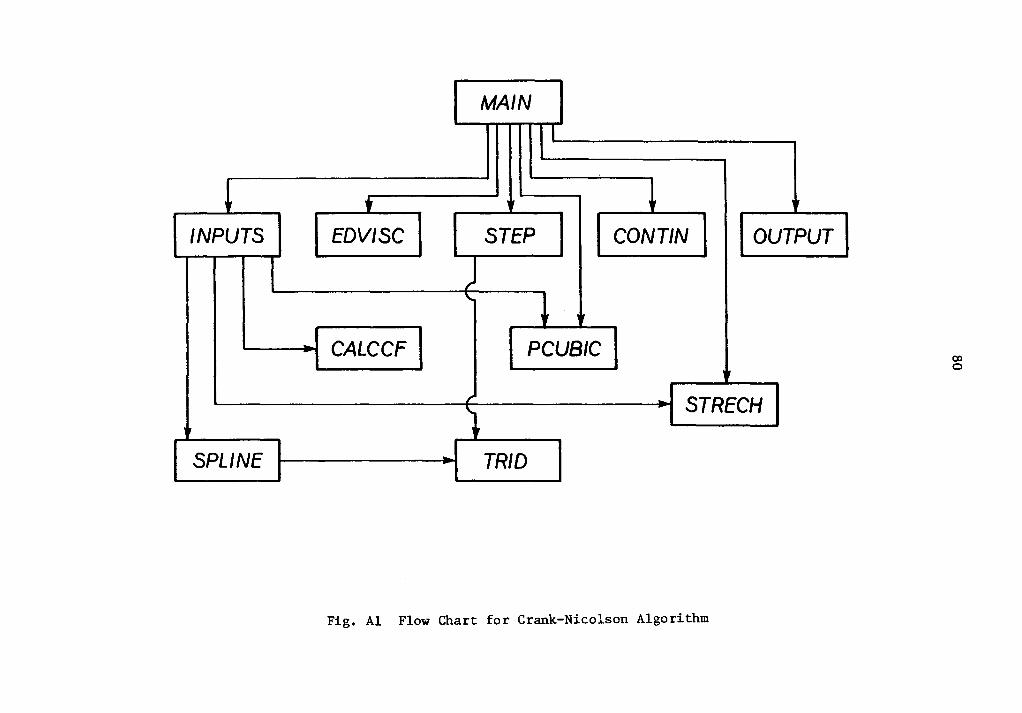
The computer code is constructed of subroutines to aid the
later user in applying and understanding the algorithm. Figure Al
shows the structure of the code. The following list is a description
of the operations performed by the various subroutines.
CALCCF
CONTIN
EDVISC
INPUTS
MAIN
Subroutine CALCCF calculates the third and fourth
coefficients (C(3,I) and C(4,I)) in the piecewise
cubic spline fit to C(l,I) utilizing the tri-
diagonal character of the matrix of coefficients.
Subroutine CONTIN solves the equation governing
conservation of mass in the boundary layer.
Subroutine EDVISC contains the eddy viscosity
model. For the laminar calculations, the eddy
viscosity is "turned off" with £=0.
Subroutine INPUTS accepts all data read into
the code. INPUTS also performs the spline fit
to the edge velocity distribution as well as
setting up the initial velocity profiles.
The program MAIN controls the flow of logic
for the Crank-Nicolson implicit finite difference
algorithm.
i INPUTS
I --
Ir
SPLINE
MAIN
I ' t I~ l I
EDVISC STEP CONT IN OUTPUT
' l ~
CALCCF PCUBIC
/ - STRECH
- TRIO -
Fig. Al Flow Chart for Crank-Nicolson Algorithm
00 0
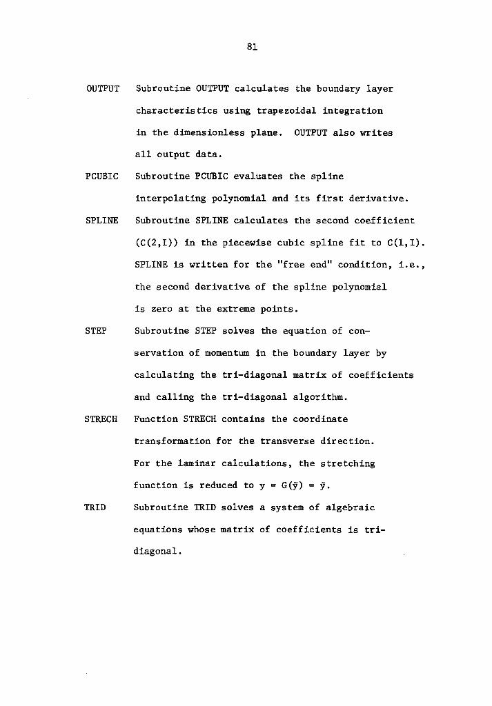
OUTPUT
PCUBIC
SPLINE
81
Subroutine OUTPUT calculates the boundary layer
characteristics using trapezoidal integration
in the dimensionless plane. OUTPUT also writes
all output data.
Subroutine PCUBIC evaluates the spline
interpolating polynomial and its first derivative.
Subroutine SPLINE calculates the second coefficient
(C(2,I)) in the piecewise cubic spline fit to C(l,I).
SPLINE is written for the "free end" condition, i.e.,
the second derivative of the spline polynomial
is zero at the extreme points.
STEP Subroutine STEP solves the equation of con-
STRECH
servation of momentum in the boundary layer by
calculating the tri-diagonal matrix of coefficients
and calling the tri-diagonal algorithm.
Function STRECH contains the coordinate
transformation for the transverse direction.
For the laminar calculations, the stretching
function is reduced to y = G(y) = y.
TRID Subroutine TRID solves a system of algebraic
equations whose matrix of coefficients is tri-
diagonal.

The vita has been removed from the scanned document
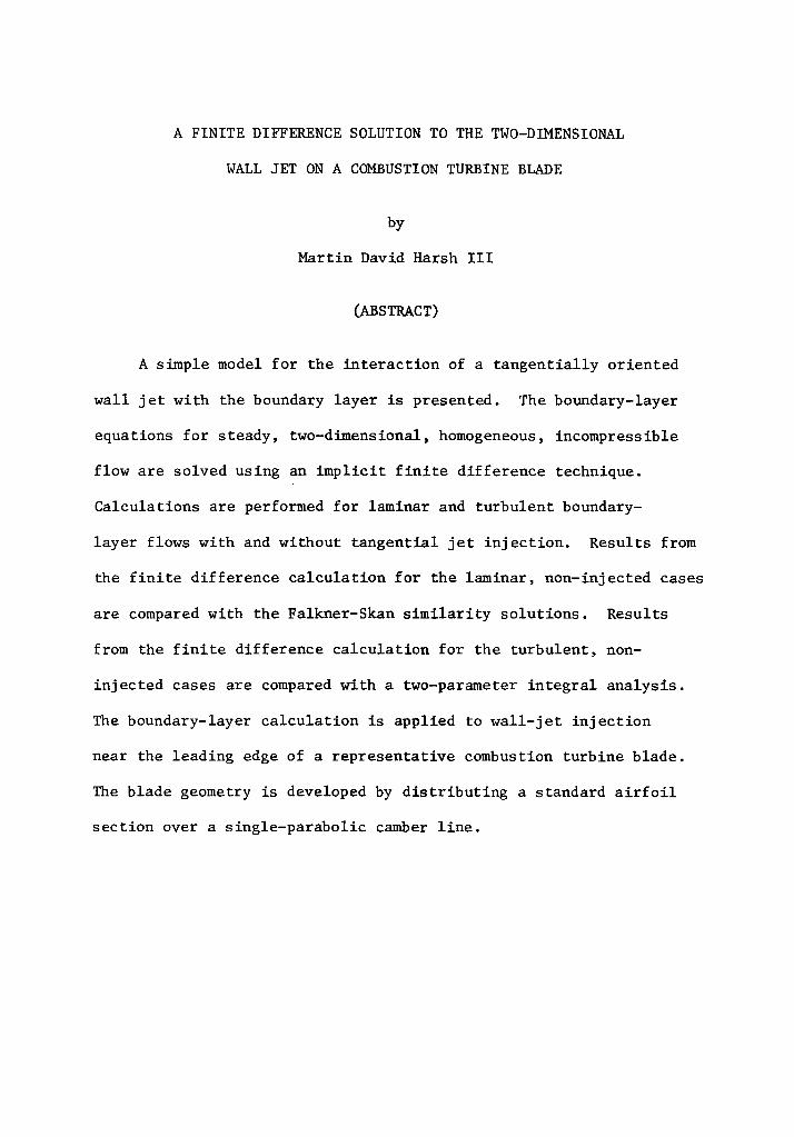
A FINITE DIFFERENCE SOLUTION TO THE TWO-DIMENSIONAL
WALL JET ON A COMBUSTION TURBINE BLADE
by
Martin David Harsh III
(ABSTRACT)
A simple model for the interaction of a tangentially oriented
wall jet with the boundary layer is presented. The boundary-layer
equations for steady, two-dimensional, homogeneous, incompressible
flow are solved using an implicit finite difference technique.
Calculations are performed for laminar and turbulent boundary-
layer flows with and without tangential jet injection. Results from
the finite difference calculation for the laminar, non-injected cases
are compared with the Falkner-Skan similarity solutions. Results
from the finite difference calculation for the turbulent, non-
inj ected cases are compared with a two-parameter integral analysis.
The boundary-layer calculation is applied to wall-jet injection
near the leading edge of a representative combustion turbine blade.
The blade geometry is developed by distributing a standard airfoil
section over a single-parabolic camber line.