Embed Size (px)
Citation preview
1
A FINITE ELEMENT APPROACH TO SPUR GEAR RESPONSE AND WEAR UNDER NON-IDEAL LOADING
By
KYLE C. STOKER
A THESIS PRESENTED TO THE GRADUATE SCHOOL OF THE UNIVERSITY OF FLORIDA IN PARTIAL FULFILLMENT
OF THE REQUIREMENTS FOR THE DEGREE OF MASTER OF SCIENCE
UNIVERSITY OF FLORIDA
2009

2
© 2009 Kyle C. Stoker

3
ACKNOWLEDGMENTS
I would first like to thank my parents for their unwavering support of all my endeavors.
Throughout my life they have always encouraged me to express my individuality and
intelligence to the best of my abilities. Without their help my successful completion of a
graduate degree would be impossible.
I would next like to thank my advisor, Dr. Nam-Ho Kim. Dr. Kim provided me with the
funding and research ideas to make this thesis possible. His constant guidance and respect for all
of his students is crucial for successful research. His professional attitude helped me to grow and
mature professionally while at the University of Florida. I would also like to thank my lab
mates, graduate professors and friends who have contributed so much to my research.
4
TABLE OF CONTENTS page
ACKNOWLEDGMENTS .................................................................................................................... 3
LIST OF TABLES ................................................................................................................................ 5
LIST OF FIGURES .............................................................................................................................. 6
ABSTRACT .......................................................................................................................................... 8
CHAPTER
1 INTRODUCTION......................................................................................................................... 9
2 LITERATURE REVIEW ........................................................................................................... 14
Current Trends in Bending Stress Analysis ............................................................................... 14Current Trends in Contact Analysis ........................................................................................... 16Current Trends in Wear Analysis ............................................................................................... 18Gear Misalignment and its Effects ............................................................................................. 20
3 SCOPE AND OBJECTIVE ........................................................................................................ 21
Problem Statement ...................................................................................................................... 21Justification of Research Uniqueness ........................................................................................ 21Usefulness of Current Research ................................................................................................. 25
4 RESEARCH METHOD AND RESULTS ................................................................................ 28
Lewis Bending and American Gear Manufacturers Association Gear Standard .................... 28Hertzian Contact Stress ............................................................................................................... 32Spur Gear Numerical Analysis Utilizing ANSYS .................................................................... 34Comparison of Numerical to Analytical Results ....................................................................... 41Two Dimensional Non-ideal Loading Conditions .................................................................... 44Three Dimensional Non-ideal Loading Condtions ................................................................... 46Archard’s Wear Model for Gear Wear ...................................................................................... 50
5 CONCLUSIONS ......................................................................................................................... 77
Conclusions of Research ............................................................................................................. 77Summary of Contributions ......................................................................................................... 77Future Research ........................................................................................................................... 78
LIST OF REFERENCES ................................................................................................................... 79
BIOGRAPHICAL SKETCH ............................................................................................................. 83
5
LIST OF TABLES
Table
page
4-1 Parameters for spur gear and pinion ..................................................................................... 56
4-2 Comparison of analytical to numerical bending stress ........................................................ 56
4-3 Comparison of analytical to numerical contact stress .......................................................... 56
4-4 Comparison of analytical to numerical bending stress 0.01” increase ............................... 56
4-5 Comparison of analytical to numerical bending stress 0.02” increase ............................... 56
4-6 Comparison of analytical to numerical contact stress 0.02” increase ................................. 57
4-7 Bending stress values for ideal 3 dimensional spur gear ..................................................... 57
4-8 Comparison of ideal 3 dimensional bending stress to out of plane translation .................. 57
4-9 Comparison of ideal 3 dimensional bending stress to b-axis rotation ................................ 57
4-10 Comparison of maximum wear depths ................................................................................. 57
6
LIST OF FIGURES
Figure
page
4-1 Beam in bending ..................................................................................................................... 58
4-2 Cantilever beam with tip load ................................................................................................ 58
4-3 Spur gear geometry ................................................................................................................ 59
4-4 American gear manufacturers association gear parameters ................................................ 59
4-5 American gear manufacturers association gear parameters cont. ....................................... 60
4-6 Hertzian contact (cylinder and gear) ..................................................................................... 60
4-7 Additional spur gear parameters ............................................................................................ 61
4-8 Finite element mesh of spur gear .......................................................................................... 61
4-9 Contact and target elements ................................................................................................... 62
4-10 Finite element analysis code hierarchy ................................................................................. 62
4-11 American gear manufacturers association gear constants and results ................................ 63
4-13 Reduced Von Mises stress plot ............................................................................................. 64
4-14 Comparison of numerical and analytical results .................................................................. 64
4-15 Spur gear contact stress .......................................................................................................... 65
4-16 Comparison of numerical to analytical results (contact stress) ........................................... 65
4-17 Non-ideal axial separation ..................................................................................................... 66
4-18 Bending stress with 0.01” axial increase .............................................................................. 66
4-19 Bending stress with 0.01” and 0.02” axial increase ............................................................. 67
4-20 Contact stress with 0.02” axial increase ............................................................................... 68
4-21 Three dimensional spur gear mesh ........................................................................................ 68
4-22 Out of plane translation .......................................................................................................... 69
4-23 b-axis rotation ......................................................................................................................... 69
4-24 Three dimensional ideal contact stress ................................................................................. 70
7
4-25 Ideal contact stress vs out of plane translation (3 dimensional) .......................................... 71
4-26 Ideal contact stress vs b-axis rotation (3 dimensional) ........................................................ 71
4-27 Normal direction for wear update ......................................................................................... 72
4-28 Finite element analysis code hierarchy for wear simulation ............................................... 72
4-29 Progressive wear; first vs. last cycle ..................................................................................... 73
4-30 Total accumulated wear depth (ideal separation) ................................................................. 73
4-31 Gear sliding distance .............................................................................................................. 74
4-32 Incremental wear profiles ...................................................................................................... 74
4-33 Wear depth superimposed on gear surface ........................................................................... 75
4-34 Progressive wear, first vs. last cycle (non-ideal separation) ................................................ 75
4-35 Total accumulated wear depth (non-ideal separation) ......................................................... 76
8
Abstract of Thesis Presented to the Graduate School of the University of Florida in Partial Fulfillment of the
Requirements for the Degree of Master of Science
A FINITE ELEMENT APPROACH TO SPUR GEAR RESPONSE AND WEAR UNDER NON-IDEAL LOADING
By
Kyle C. Stoker
May 2009 Chair: Nam Ho Kim Major: Mechanical Engineering
Spur gear response and wear is an engineering problem which has been around for
hundreds of years. The method to determine stresses analytically has been developed
extensively by the American Gear Manufacturers Association, and experimental techniques
investigating wear of spur gears is well documented. Currently engineers design gears based on
a fixed safety factor which determines the lifetime of a gear based on predictable loads and
stresses. Additionally, all mechanical assemblies are subject to tolerances that limit the amount
of error between physical components. When assemblies are operated at the limits of these
errors, stresses and wear will increase.
This research has provided the engineer with a tool to predict where and by how much the
stresses of spur gears will increase when non-ideal conditions are present for both 2 dimensional
and 3 dimensional analysis. A wide range of spur gears can be input to the parametric code and
the Finite Element Analysis program will solve the contact problem and produce valid results. A
method to predict progressive wear evolution for a 2 dimensional spur gear according to
Archard’s wear law has been implemented within the FEA code. The research has shown that
with an increase in the axial separation wear depths will increase and the wear profile will be
modified.
9
CHAPTER 1 INTRODUCTION
Gears are an integral and necessary component in our everyday lives. They are present in
the automobiles and bicycles we travel with, satellites we communicate with, and computers we
work with. Gears have been around for hundreds of years and their shapes, sizes, and uses are
limitless. For the vast majority of our history gears have been understood only functionally.
That is to say, the way they transmit power and the size they need to be to transmit that power
have been well known for many years. It was not until recently that humans began to use
mathematics and engineering to more accurately and safely design these gears.
Wilfred Lewis introduced a method to calculate the amount of stress at the base of a gear
tooth in 1892. His method was based upon a cantilever beam which was subjected to a load at
the tip of the beam. Although this method was crude, it remains one of the bases for gear design
to this day. Heinrich Hertz began his own work on contact pressures around the same time in
1895. His research on the elastic contact of two cylindrical bodies allowed engineers to calculate
the contact pressure between a gear and a pinion. With these tools engineers were able to better
predict the bending stress and contact pressures of gear pairs to allow for more robust design.
Continuing with this trend gear design engineers sought to reduce the overall weight and size of
gear pairs while still maintaining a high level of safety. In this discussion, safety is defined as
the ratio of actual stress to allowable stress. If this ratio exceeds one, the component will fail.
Many organizations, including the American Gear Manufacturer’s Association (AGMA) have
sought to standardize the gear design process by developing their own formulas for gear design.
The major changes over Lewis’ original equations are the ability to take into account the
geometrical complexity of the gear tooth, as well as the actual location of the contact.
10
With the advent of Finite Element Analysis and Computer Aided Design (FEA and CAD)
the ability to quickly and accurately design gears has been greatly improved upon. With modern
CAD programs a typical gear and pinion can be modeled relatively easy. With better computing
power, FEA software can quickly and efficiently analyze the stresses and contact pressures in
gear pairs. These tools make the design and analysis stage much cheaper and faster for the
design engineer. Because actual experiments are costly and take large amounts of time, a
repeatable and accurate design tool is crucial for real world application.
With the advent of tighter tolerances and more demand to produce lightweight structures
small deviations in tolerances can cause gears to fail before their specified lifetime. These
deviations are present in any mechanical system and are prescribed by the engineer. Typical
tolerances can change in any of the three principal directions by as much as 0.02", or 0.508 mm.
Within this small window of allowable tolerances drastic changes in bending stress and contact
pressure can occur. As the distance between the gear and pinion’s axis of rotation increases the
bending stress and contact pressure rise. A relatively small rise in bending stress can cause a
gear tooth to fail at lower cycle numbers than the design calls for. With an increase in the
contact pressure between a gear and pinion wear will be increased as well. With increased wear,
gear failure may occur sooner by pitting, corrosion, and adhesive wear. Much work has been
done experimentally over a wide range of circumstances. The effect of higher torques on the
load carrying capabilities of gears has been extensively studied to determine the allowable
operating conditions. In addition to higher torques, higher operating speeds have been
experimented with to see how the wear regime may change from oxidation wear to bulk wear.
Because of these extensive studies and experiments many gear manufacturers today use case
11
hardened gears to alleviate the harmful effects of high contact pressure. These hardened regions
of the gear tooth allow for higher contact pressures without the detrimental effects.
Although much study has been done on the mechanisms of gear wear and the major
contributors to that wear, there is still a lack of understanding when it comes to the tolerances
and how they affect the wear characteristics. Inherent in any mechanical system will be a small
window of allowable space that the gears can be assembled in. In worst-case scenarios these
small windows of tolerances may “stack up” to produce an overall large deviation from ideal
assembly. With modern CAD and FEA software the input of these tolerance deviations are
relatively simple, cheap, and repeatable. The purpose of this research is to provide a parametric
gear design code capable of introducing these tolerance anomalies, or “non-ideal conditions”.
The program can quickly and accurately model a real world gear and pinion and introduce a
variety of non-ideal conditions. With these non-ideal conditions in place the gear and pinion will
be rotated and the contact pressures and bending stresses compared to the ideal case. We will
see that both the contact pressure and bending stress will increase as these conditions are
imposed. One important discovery was that with minimal changes to the axial separation
between the gear and pinion contact pressures can drastically increase over a portion of the
rotation due to a decrease in the load sharing capabilities of the gear pair. This phenomenon will
be discussed more in depth in Chapter 4.
In addition to developing a parametric tool capable of predicting where and by how much
bending stress and contact pressures increase due to tolerance errors, this program will also be
able to predict the wear profile over thousands of cycles. This was accomplished by designing
an FEA code that selectively modifies nodal locations according to Archard’s wear model. As
the non-ideal conditions are introduced the contact pressure between the gear and pinion was
12
found to increase. Because Archard’s wear model is directly proportional to the contact
pressure, the predicted wear will increase. Also, as the non-ideal conditions are imposed the
sliding characteristics of the gear and pinion are modified. This program is able to capture these
geometric effects and include them within the wear regime. This research will provide an
efficient and repeatable process which will determine where and by how much the wear will
change and the effect this has on the predicted life cycle of the gear.
The final stage of this research proposes a relatively simple experimental set-up that
could be designed and built to validate these results. Typical gear test rigs available for purchase
can range in excess of $10,000. For most applications this exorbitant price eliminates the
possibility of on-site testing. A much simpler and pragmatic solution is proposed that has a total
cost of under $1,000. The capabilities of this rig would be two-fold. One, the test rig will be
able to provide an input torque to a drive gear, which turns the driven gear. After a pre-
determined set of cycles the amount of wear in two nylon gears can be determined by a mass
measurement. The second part of the experiment would be to introduce the non-ideal conditions
to investigate how the amount of wear is affected. The purpose of this would be to validate the
theoretical results.
This discussion will continue with a review of the current and past practices for gear
design in Chapter 2. Literature reviews of the current trends and practices for gear design and
analysis will also be included. Chapter 3 will concisely state the contribution of this work to the
engineering community, and justify the originality of this research. Chapter 4 is the main body
of this thesis and will include the procedure and methods for obtaining the results. Chapter 5
focuses on the specific conclusions and the contribution of new knowledge. Some future

13
research recommendations will also be made pertaining to additional wear analysis and an
experimental test rig.
14
CHAPTER 2 LITERATURE REVIEW
Current Trends in Bending Stress Analysis
Until the mid 20th century all gear design was based upon Lewis’ original bending equation
[1,2]. Lewis based his analysis on a cantilever beam and assumed that failure will occur at the
weakest point of this beam. Lewis considered the weakest point as the cross-section at the base
of the spur gear. However, failure due to flexural stresses on bodies with changing or
asymmetrical cross-sections was proved inaccurate by Dolan and Broghamer [2]. Their
approach used photoelastic experiments to visualize the stress concentrations due to the fillets at
the base of spur gears. By these visualization techniques they were able to more accurately
predict at what stress levels gears will fail due to high bending stresses. Much early work was
done using photoelastic experiments to design spur gears based on the stresses observed at the
most critical points [3]. The correct placement of keyways in relation to gear teeth as well as the
maximum acceptable diameters was recommended. While these methods were useful in
determining static stresses in spur gears, the photoelastic trend moved toward dynamic analysis
[4]. Dynamic photoelastic analysis allowed scientists to document the scattered stress values due
to gear vibration and power transmission. With this continuing trend of experimental bending
stress analysis the American Gear Manufacturers Association (AGMA) published their own
standard based on Lewis’ original equation [5]. Established in 1982, this standard is still widely
used in gear design today [6]. The current trend is to more accurately compute and predict the
geometry factors which are critical in determining bending stresses for a wide variety of gears
[7]. These geometry factors account for the changing shape of the gear tooth, the point where
the load is applied, as well as the fillet radius at the tip and base of the tooth.
15
Until the mid 1980’s the majority of spur gear design and bending analysis was still being
done by hand. Although Finite Element Analysis has been around for over half a century, it was
not until computing power increased that the real advantages of this method became apparent.
With the advent of more powerful computers the ability to analyze and describe the stress state
of spur gears increased dramatically. One of the first mentions of Finite Element Analysis with
respect to spur gears [8] identifies the importance of this type of analysis. Early FEA of spur
gears was very labor intensive for the engineer. The first challenge to overcome was properly
modeling the spur gear to capture the correct geometry. Once the geometry has been modeled
the types of elements and mesh is crucial. Areas where higher stresses and deformations occur
needed to be meshed more densely so that the results were accurate. Many of the first attempts
of FEA on spur gears were modeled in 2-dimensions to simplify the solution. Beginning in the
early 1990’s many attempts were made to analyze the stresses of spur gears using 3D FEA [9].
Again, the accepted method was to accurately model the spur gear, appropriately mesh the gear,
and analyze the bending stress. The advantage of this method over experimental techniques is a
more cost effective and repeatable result can be obtained. By verifying that the FEA results
correspond closely to experimental results the validity of this type of method has also been
confirmed. Modeling spur gears and analyzing the results using the Finite Element Method has
led to many insights which may not have been immediately apparent. With dynamic analysis,
authors have noted that impact loads can be as much as 1.5 times that of static loads, which is of
great importance when selecting appropriate gears [9]. Others have observed how the
transmission error of spur gears is affected by the size and shape of the gear tooth profile [10].
The current trend of gear design is becoming more focused on designing different shaped gears
to transmit higher loads without failure. The purpose of this method is to more precisely
16
engineer these gears so that the maximum efficiency can be achieved. By changing the shape of
the gear tooth to an asymmetrical design the authors have proven a decrease in both bending
stress and contact pressure [11].
With the ability to accurately and cost effectively model spur gears and obtain accurate
bending stress results engineers are attempting to reduce the size of the gears so that cost and
weight can be minimized. Current gear design utilizes a safety factor when determining the
allowable stress versus the actual stress, and safety factor values can be quite high depending on
the application. High safety factors would mean that the stress that the gear tooth can transmit is
much higher than the actual stress the tooth will ever be exposed to. While this type of design is
desirable for longevity and reliability the cost of manufacture and assembly is inherently
increased due to extra material and machining costs. Recent attempts to design the gears based
on safety factor matching was introduced [12]. By defining allowable limits for safety factor and
other tolerances the authors were able to again modify the shape of the gear to reduce stress in
critical regions.
The current trend of gear design focuses on minimizing the bending stresses encountered
at the base of the spur gear. To aid in this design FEM has taken a strong role as a tool to help
identify critical areas. One of the focuses of this research will be to develop an FEA tool which
is capable of modeling spur gears. Improvements on some existing work will be introduced as
the ability to parametrically modify the gear dimensions. By inputting the correct dimensions for
any spur gear an accurate model can be created. In addition to modeling spur gears the program
will also be able to quickly and accurately measure the bending stress of the spur gear.
Current Trends in Contact Analysis
In addition to the previously mentioned research the contact pressure at the point of mesh
between gear and pinion is of great importance. Archard was one of the premier scientists to
17
experiment with contact pressure between two deformable bodies in the 20th century [13]. His
work led to many of the modern techniques and formulations that are present today for contact
analysis [13,14]. His theory expanded upon the works of Heinrich Hertz, who calculated the
contact pressure between two deformable cylinders [15]. In much the same way as the bending
stress between the gear and pinion was investigated, the contact pressure was investigated as
well. The difference between the two is that the contact pressure analysis is much more
straightforward than the bending stress analysis. While the bending stress is dependant on the
geometry and shape of the gear tooth, the contact pressure is mainly a function of the type of
material in contact and the radius of curvature [16]. There has been some research into the
contact pressure between a spur gear and pinion, and asymmetrical gearing has again been
proven useful. The authors of this study were able to design asymmetrical gears to increase the
load carrying capacity as well as reduce the overall weight of the system [17]. FEM approaches
were used in their research and the results are well documented. Also related to the contact
pressure is a vast amount of work on the stiffness of spur gear teeth and the appropriate method
of modeling using FEA [18]. Their work has proved the non-linearity present at the beginning of
contact between teeth, as well as the importance of the point of contact. Although the contact
pressure problem has been solved and the accuracy validated, there remains much work to be
done on the analysis of spur gears when improperly aligned. Properly aligned spur gears are
designed to mesh with the pinion at a precise point. This point is known as the “pitch point” and
provides the maximum amount of power transmission between gear and pinion. Although
contact pressures can be high at this point, the metal on metal sliding is theoretically zero.
Because of this condition the wear at this point will be low. If the point of contact is modified
due to errors in assembly the contact pressure can increase because of geometric differences
18
between the gear and pinion. This phenomenon will be discussed in Chapter 4. In addition to
higher contact pressures, the amount of sliding between gear and pinion will increase and cause
the wear to increase as well.
Current Trends in Wear Analysis
There are many mechanisms which are influenced by contact pressure. One of the most
important in gears is the amount of wear that is observed on the surfaces of the gear and pinion.
This relationship is directly proportional and was first proposed by Archard [19]. Archard’s
approach utilizes the relationship between contact pressure and sliding distance along with a
unique wear constant to predict the amount of material that would be removed when two metallic
objects are in contact. Early experimentation was concerned with the amount and location of
wear between lubricated gears [20]. The main focal point of these experiments was to determine
the cause of gear failure as it is related to gear wear. Failure from wear can be defined as pitting,
corrosion, bulk wear, scoring, and creep. By understanding the process with which wear occurs
engineers design spur gears with those considerations in mind. One of the most well
documented wear regimes is the tendency for wear to occur mainly at the tip and root of the gear
[21]. This is related to Archard’s wear model because of the geometry of the spur gear. Wear is
proportional to the contact pressure as well as relative sliding between the two materials. At the
optimal point of contact, known as the “pitch point”, there is relatively little sliding. The
maximum amount of power is transmitted between the gear and pinion at this point, and
engineers plan on this when designing the shape of spur gears. The shape is known as an
involute curve and is crucial for minimal wear between gear and pinion.
As the ability to understand the complex wear processes increased the emphasis on
experimentation and theoretical analysis grew increasingly popular. One of the most prevalent
and accurate methods to measure gear wear was developed using the FZG gear test rig [22].
19
This experimental test rig can accurately apply a torque to a shaft which rotates a gear and
pinion. The gears can be either lubricated or un-lubricated and the amount of wear is measured
by precise mass measurements. Typically, the profile of the gear tooth is measured by a probe to
determine the wear depth along the tooth. One important experimentation was conducted by A
Flodin and S Andersson [23]. The authors used an FZG rig to study mild wear in spur gears. A
known phenomenon in the gear industry is the initially improved contact conditions which are
generated as wear just begins to occur. This is generally attributed to small imperfections and
roughness on the surface of gear teeth being worn away. Their study proved the observed
phenomenon of locally high contact pressures being reduced by the improved contact conditions.
Another important landmark for this study was the use of the “single point” observation method.
By following the contact pressures and wear depths at a single point a repeatable trend can be
observed. They proved their experimental results with a numerical simulation as well.
Archard’s wear equation has been further validated by studies employing Signorini’s contact law
and Coulomb’s law of friction to spur gear wear analysis [24]. Further studies have included the
dynamic effects of wear to the analysis [25]. By generating an accurate geometrical model
depicting spur gear wear the authors showed that the gear ratio can change, which will cause a
modification of the durability of the gears in real world application. Other studies have been
done on wear of helical gears [26], nylon gears [27], and coated gears lubricated with
biodegradable lubricants [28]. The common thread between all of these studies is clear. The
need to accurately model spur gears and correctly predict progressive wear is crucial in the
design of gears. Without including progressive effects the safety factor and allowable lifetime of
the gear can be affected. Increases in contact pressure and bending stress will invariably lead to
more wear and fatigue damage.
20
Gear Misalignment and its Effects
One topic that has not been discussed thoroughly is the effect of “non-ideal” loading
conditions on the wear of spur gears. Non-ideal conditions are characterized by a change in the
tolerances or specifications which define the acceptable assembly of a gear train. Some studies
have been conducted on how the noise or vibration of spur gears are affected by manufacturing
error (tooth surface roughness) or misalignment [29,30], although there was no mention of how
this could affect wear. Another study modeled face gear drives and the increase in contact
pressure and bending stress when misaligned [31]. Their study observed significant increases in
the contact pressure, as well as reduction in the load sharing effects of the teeth. Their
recommendations include a more simplified modeling procedure and mesh algorithm to reduce
the amount of modeling time. They also suggested including additional misalignments to
properly provide guidelines for gear design. One recent study of spur gear misalignment and
machining errors confirmed these results [32]. To date, the author has not seen any research on
the effects of these misalignments on the bending stress and contact pressure as it pertains to the
amount and location of wear. By accurately modeling a spur gear in mesh, introducing
misalignments and non-ideal conditions, and predicting the resultant progressive wear using
FEM an innovative and valuable design tool will be produced.
21
CHAPTER 3 SCOPE AND OBJECTIVE
Problem Statement
The main purpose of this research is to provide a parametric spur gear design code which
has the ability to predict progressive wear evolution, bending stress increase, and contact
pressure increase when subjected to non-ideal loading conditions. These non-ideal loading
conditions are defined by accepted engineering tolerances imposed on real mechanical structures.
As the normal life cycle of the mechanical system progresses the outer limits of these tolerances
will be experienced in some cases. Due to higher stresses and contact pressures the wear will
increase along the profile of the gear tooth. This research will provide an engineer with the
ability to better design and specify spur gears which are expected to experience these conditions.
The ability to more precisely engineer gears closer to a safety factor of one will save
manufacturing and materials cost. By better understanding the process which leads to ultimate
failure a more reliable and better engineered product can be produced.
Justification of Research Uniqueness
In the past there has been some research into the transmission error as gear trains operate
[33]. In Chapter 2 the studies done on how the noise and vibrations of gears are affected by
misalignment and tooth roughness were also documented [29,30]. The authors in this paper [34]
noticed the inherent lack of research in the contact fatigue analysis of gears. Although their
research proposed an experimental method to determine how shot-peening may reduce the
amount of cracks and surface fatigue experienced on gear teeth, their focus calls for an
understanding of the process as it occurs. Another experimental study notes that extremely high
pressures and stresses can result from a small misalignment of the gear shafts [35]. Fatigue
failure due to misalignment of shafts is generally a sudden phenomenon with no warning.
22
Depending on the amount of misalignment, the gear may fail after a relatively short amount of
time, or the gear may last longer. Another study involved a pinion which had failed in service
[36]. The conclusion of this study was that the misalignment and improper heat treatment of the
gear was fully responsible for the failure. Their recommendations include ensuring that the gears
are properly aligned as well as an ability to measure the torque as the gears are in service. One
NASA study suggested that an ability to optimize the gear tooth shape to lower contact
pressures, as well as a numerical method to diagnose the remaining lifetime of a gear train would
be valuable [37]. Tools capable of predicting the remaining lifetime of a gear train assembled
within specific tolerances would be useful for this type of application. To this date there have
been many experiments and research studies on spur gear analysis. Searching “spur gear” on a
journal article search engine yields over 42,000 hits. Spur gears themselves have been around
for thousands of years as well. As the understanding of the dynamics and mathematics of these
gears progressed the ability to better engineer their design improved. Lewis and Hertz were
some of the founding fathers of modern gear design technology and their influence is no doubt
still felt to this day. Beginning in the early 20th century the understanding of these gears had
increased enough to allow for a more thoughtful design. By studying the mechanics behind
stress concentrations, metallic wear, and fatigue failure a standardized approach to gear design
began to emerge. As experimental techniques improved the ability to justify these equations
were first realized by photoelastic experiments. The actual location and severity of the stress
increases could be determined even as the gears themselves rotated. With this new
understanding of where the maximum stress and contact pressure was occurring engineers were
able to better design their gear trains. They decided on allowable tolerances for the shafts on
which these gears were rotating, as well as minimum thicknesses and diameters for the gears
23
themselves. As even more research was being conducted in the 1950’s a new approach was
emerging. Finite Element Analysis began as a somewhat limited field of research. Engineers
realized the powerful capability of this new field, but were unable to realize its full potential.
Experimental techniques were still being improved upon and the wear mechanisms which
influenced the eventual failure of the gear teeth were better understood. Archard introduced his
unique contribution to the wear community by capturing the basic components of wear behavior.
By developing a wear constant he was able to relate the wear depth to contact pressure and
sliding distance. Experimental rigs such as the FZG spur gear test rig were developed to validate
his results.
As computing power increased the FEA approach was again revisited. Engineers realized
that by accurately modeling real world gears in a computational environment, the finite element
equations could be included to analyze static loads. Once the validity of this approach was
confirmed the trend moved toward dynamic analysis. The effects of impact loading, gear tooth
geometry, and types of lubrication were all considered. With the results of the finite element
analysis engineers were able to avoid detrimental engineering decisions which would ultimately
cause the failure of the gear tooth. Finite element methods began to see use as an optimization
tool where the tooth geometry could be modified to reduce the bending stress and contact
pressures.
Current research of spur gears is focused on avoiding premature failure and understanding
the cause of this failure. By designing spur gears closer to a singular value for the safety factor,
costs can be reduced dramatically. The reduction of these costs will be realized through less
material being used in gear manufacture, as well as a better understanding of when and where
maintenance should be preformed.
24
The originality of this research stems first from its parametric design. Some parameters
inherent to every spur gear have been identified and separated from the gear code which
generates the geometry. Any feasible spur gear design can be simply input into this separate file
and a new spur gear can quickly and efficiently be modeled. The design engineer will not have
to spend countless hours modifying or correcting existing models. With this parametric
capability numerous spur gear designs can be thoroughly investigated which can be applicable to
a wide variety of industries.
Some preliminary research has been conducted on how misalignments of gear shafts can
affect the bending stress and contact pressure. The vast majority of this work has been done
experimentally and there exists no standardized method of analytical study. With a parametric
program the input of these non-ideal conditions is trivial. By identifying the typical tolerances
present in today’s mechanical systems the limits of these conditions have been studied in this
research. There are three major non-ideal conditions which will be considered in this research.
The first is the axial separation between the centers of rotation of a spur gear and pinion. The
second is an out of plane translation of the spur gear and pinion. The final non-ideal condition is
a rotation about the b-axis. The b-axis is analogous to a rotation around the y-axis. Hence, “a”
and “c” rotations occur about the “x” and “z” axes. Although there has been a large number of
studies conducted on how the bending stress and contact pressure are altered by conditions such
as these, the majority involves experimental results. The authors mainly comment on specific
instances and gears without providing a useful analysis tool. This research is unique in the fact
that a repeatable and efficient computer code is generated to fully analyze these non-ideal
conditions. By a better understanding of the mechanics involved when gears are operated under
these conditions a better design can result.
25
The final original contribution of this research to the engineering community is its ability
to predict the amount of wear in 2 dimensions. Archard’s wear model is used in this wear
prediction and progressive wear is considered. Progressive wear is defined as the ability of
previous wear to impact the contact pressures of the current cycle and modify the wear profile
accordingly. Much experimental analysis has been conducted on the wear characteristics of spur
gears. The types of wear have been studied extensively and the manner in which this wear
causes gear failure has been documented. This research is unique in that the effect that non-ideal
loading conditions have on the amount of wear is emphasized. Although it is known that a spur
gear will wear out, little research has been conducted on how the increasing contact pressure due
to non-ideal conditions will affect future life cycle predictions. This research will shed light on
the severity and location of wear increase due to non-ideal loading so that engineers can plan for
this phenomenon according to the specific application of each gear set.
Usefulness of Current Research
The usefulness of this research will be most applicable to the gear design community. As
mentioned in Chapter 2, the current trend of gear design and analysis is most assuredly focused
on the reduction of cost while maintaining the same level of accuracy and reliability. In the past,
the method to ensure reliability was often to over design the gear and pinion. Over design refers
to the use of more material or tighter tolerances to ensure that the gear train will not fail before
the expected lifetime of the part. While this method ensures reliability it does not
advantageously affect the cost of manufacture and assembly. As each engineering application is
unique, so too should be the types of gears and the tolerance requirements for each case.
With the advent of higher performing CPU’s, the extension of FEA to gear design was
inevitable. As mentioned previously, this research will provide the engineer with a tool to
quickly change gear parameters and study how non-ideal conditions will change the way the gear
26
behaves. This behavior is captured in three separate but interrelated phenomena. This research
will first be able to quickly measure the severity and location that bending stress increases due to
non-ideal loading. This will be useful to the engineer when specifying the thickness and size of
gear teeth. If for example, a tolerance of 0.001” is mandatory for a specific application the
design engineer can quickly calculate how much fluctuation in bending stress is expected.
Depending on this value different materials and sizes of gears can be more precisely determined.
The more understanding the engineer has on how tolerances and assembly affect the gear
response, the better.
Along with being able to quickly determine how bending stresses increase, the
corresponding increase in contact pressure can be studied as well. Because spur gears are
designed using an involute curve the location of contact is crucial. To understand what an
involute curve is, imagine a strip of thin sheet metal wrapped around a cylinder of any diameter.
If you were able to unwrap this piece of stiff metal from the cylinder, the curve that the end of
the strip of metal generates in space would be known as an involute curve. This will be
discussed more fully in Chapter 4. The main advantage of using involute curves in spur gear
design is that at the pitch point the relative sliding between gear and pinion will be minimal.
Because relative sliding between metals is necessary for wear to occur, this minimizes the wear
depth. In addition to this, the maximum amount of power is transmitted from the drive gear to
the driven. When the axial separation or b-axis modifications are introduced this advantageous
effect will no longer be present. Because of this the contact pressure can increase substantially,
causing localized stress intensities. Theses high values of contact pressure will cause the gear
train to fail sooner than expected. At the outcome of this research the ability to better understand
27
this situation will be provided. Depending on the application, the design engineer can decide
how crucial tolerances for his or her specific gears are.
The aspect of this research that is most useful is the ability to predict the progressive wear
evolution, especially when non-ideal conditions are present. The amount of research conducted
on spur gear wear has been documented in Chapter 2. For over 60 years there have been
numerous experimental studies on the effects of lubrication, tooth shape, and operating
conditions on the amount of wear. Attempts have been made to modify gear tooth shape based
on these observations. Along with experimentation there have also been many analytical studies
on spur gear wear. These analytical studies all employ some type of finite element method to
determine the contact pressures of spur gears accurately. The attempts to then model the wear
have been minimal, and most of the contributions have come from Anders Flodin. His methods
have validated the relationship between finite element predictions and the real wear regimes that
are evident in spur gear drives. The new contribution to this already established research will be
the addition of the non-ideal loading conditions. All types of spur gear assemblies are subject to
tolerance specifications. The level of accuracy in manufacture and assembly is directly
influenced by these specifications. This research will provide engineers with the ability to
quickly determine how these tolerances affect the amount and location of wear. With better
engineering techniques and analysis the failure of spur gears due to bending stress has been
decreased. The majority of failure occurs due to wear, and this research will provide a direct
correlation between tolerances and gear wear. For each specific application the effects on wear
can be predicted. This will be useful as the trend of gear design continues towards a more cost
efficient product. By fully understanding the process of wear and how wear regimes may change
due to non-ideal conditions a robust and efficient tool has been developed.
28
CHAPTER 4 RESEARCH METHOD AND RESULTS
Lewis Bending and AGMA Gear Standard
As mentioned in Chapter 2 the basis for bending stress analysis of spur gears is based upon
Wilfred Lewis’ original formulation. His theory began with the basis that a spur gear can be
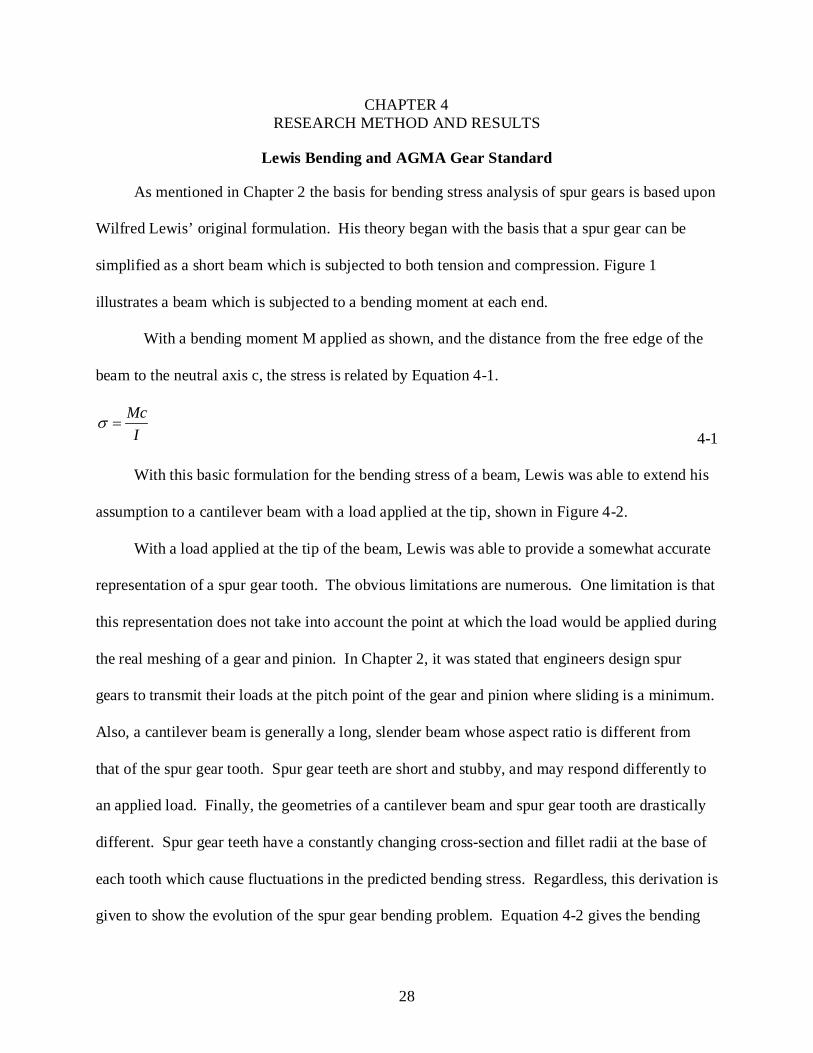
simplified as a short beam which is subjected to both tension and compression. Figure 1
illustrates a beam which is subjected to a bending moment at each end.
With a bending moment M applied as shown, and the distance from the free edge of the
beam to the neutral axis c, the stress is related by Equation 4-1.
McI
σ = 4-1
With this basic formulation for the bending stress of a beam, Lewis was able to extend his
assumption to a cantilever beam with a load applied at the tip, shown in Figure 4-2.
With a load applied at the tip of the beam, Lewis was able to provide a somewhat accurate
representation of a spur gear tooth. The obvious limitations are numerous. One limitation is that
this representation does not take into account the point at which the load would be applied during
the real meshing of a gear and pinion. In Chapter 2, it was stated that engineers design spur
gears to transmit their loads at the pitch point of the gear and pinion where sliding is a minimum.
Also, a cantilever beam is generally a long, slender beam whose aspect ratio is different from
that of the spur gear tooth. Spur gear teeth are short and stubby, and may respond differently to
an applied load. Finally, the geometries of a cantilever beam and spur gear tooth are drastically
different. Spur gear teeth have a constantly changing cross-section and fillet radii at the base of
each tooth which cause fluctuations in the predicted bending stress. Regardless, this derivation is
given to show the evolution of the spur gear bending problem. Equation 4-2 gives the bending
29
stress relation when the values for the second moment of inertia I are substituted into Equation 4-
1, where L is the length of the beam, t is the thickness, F is the face width, and W is the point
where the load is applied.
2
6Mc WLI Ft
σ = = where
3
12FtI =
4-2
Equation 4-2 was used for the initial analysis of spur gears and it was soon realized that
this equation was not valid for most types of spur gears. In order to have an accurate
representation of the spur gear response it is necessary to include the relevant geometrical
parameters which influence the bending stress. Because of the complexity of these parameters,
the basic geometry of the spur gear will first be introduced. Then, a more detailed view of a
single spur gear tooth will be given and the derivation of the bending stress explained.
Figure 4-3 represents the typical geometry which is present on a spur gear. The circular
thickness is analogous to t in Equation 4-2, the face width is analogous to F, and the length of the
tooth is the distance from the fillet radius to the tip. The region of interest for bending stress is at
the very bottom area of the spur gear. Because of the transition from a relatively wide and thick
tooth to a narrow base, this area experiences the greatest compression and tension on the tooth.
Although the area in compression will have a higher magnitude of stress, gear failure typically
occurs in tension due to the formation of cracks. While compression acts to push cracks
together, the tension continues to grow the cracks by pulling them apart. Also, the line labeled
“circular pitch” is the diameter on which the majority of contact should occur. This ensures that
the maximum amount of power is being transferred, with the minimum amount of slipping.
Now that the geometry of the spur gear has been introduced, it is necessary to define
additional parameters which will be used to fully capture the geometry of the spur gear tooth. By
30
solving for these geometrical parameters the most accurate analytical solution of the bending
stress and contact pressure can be achieved.
Figure 4-4 will be referenced throughout the derivation of the AGMA bending stress
equation. This derivation is derived in part from [38]. First, a bending stress equation similar to
Lewis’ original is given. For this equation both the bending and radial stresses are shown:
( )( )( )3
cos1 1 2
12
w Dbending
w x x y
y
γσ
−= 4-3
( )( )sin
1 2w
radialw
yγσ = 4-4
In Equation 4-3, ( )cos w Dw x xγ − is the load w, inclined at angle γw
sin ww γ
, multiplied by the
distance from the base of the tooth to give the bending moment. Y is the distance from the
center line to the edge of the gear tooth. The remaining portion of Equation 4-3 is the second
moment of the area. Equation 4-4 uses the radial force along with the thickness 2y to
produce the radial stress. Stress concentration factors were introduced in the 1950’s to calculate
a factor based on geometrical features which would modify the expected stress values [39]. For
spur gears, the most important stress concentrator occurs at the base of the spur gear tooth.
Equation 4-5 gives the stress concentration factor Kf
2 3
12 2
k k
ff D
y yK kr x x
= + −
.
4-5
In Equation 4-5, k1, k2, and k3
( )( )( )
21
22
23
0.3054 0.00489 0.000069
0.3620 0.01268 0.000104
0.2934 0.00609 0.000087
s s
s s
s s
k
k
k
φ φ
φ φ
φ φ
= − −
= − −
= − −
are all constants given by Dolan and Broghamer in their
initial photoelastic experiments [40].
4-6
31
In Equation 4-6, φs is the pressure angle, a constant specified for all gears. For this case
the pressure angle is 20º. Rf
( )2
( )r rT
f rTsg r rT
a e rr r
R a e r− −
= ++ − −
is the fillet radius of curvature, and is given by Equation 4-7.
4-7
Figure 4-5 is a schematic of how the radius of a gear tooth is formed. In Figure 4-5, A is
the gear tooth being generated, and B is the rack cutter. Rsg is the radius of circles centered at
the gear axis, for the standard gear. RrT is the radius of the section on the gear tooth cutter which
forms the gear fillet radius. Ar
( )2
max
1.5 .5 tancos D wt w f
m x x mw Km y y
γσ γ −
= −
is a point on the radius of the rack cutter which is doing the
actual cutting. Finally, e is a profile shift that is necessary for the rack cutter to be in the proper
position to cut the gear tooth fillet. Combining Equations 4-3 through 4-7 yields the final form
of the fillet stress formulation.
4-8
The only term not defined in Equation 4-8 is the module m.
rpmπ
= 4-9
In Equation 4-9, pr is a constant known as the rack pitch. Equation 4-8 will be the basis
for the analytical bending stress of the spur gear. This equation takes into account the individual
geometry of each spur gear, and gives an accurate result for the maximum bending stress. This
maximum bending stress is based on x and y locations along the fillet radius of the gear tooth.
Equation 4-8 will be used to prove that the results gained from the numerical analysis are
consistent with stresses encountered in reality.
32
Hertzian Contact Stress
The contact stress or contact pressure will be used interchangeably throughout this paper.
Either term refers to the amount of stress at the point where a gear and pinion are in mesh. As
will be discussed in subsequent subchapters, the value of the contact pressure is extremely
important when attempting to predict the amount of wear depth that will occur as the gears
rotate. The derivation of this equation was first performed by Henrich Hertz in the late 1800’s.
Hertz’s approach is a derivation based upon the elastic contact of two cylinders. When two
cylinders are in contact their contact profile is defined by a line. This analogy can be applied to
the point of contact between a gear and pinion. Because the profile of a spur gear tooth is
defined by an involute curve, the radii of the cylinder which generated the curve and the radius
of curvature of each tooth is the same. Figure 4-6 will clarify this proposition.
The Euler-Savary equation proves the relationship between a circle, whose center is
denoted as “E”, and the point of contact A which momentarily corresponds to that circle. Then,
the radius of curvature ρ of the involute at point A is equal to the length EA and is given by
Equation 4-10.
tanb REA Rρ φ= = 4-10
This idea was derived by a combination of the following two sources [38,41]. With the
proof that the instantaneous radius of curvature of the involute curve will be equal to the radius
of curvature of a cylinder in contact with another cylinder, the contact stress derivation can
continue. In reference to the two cylinders in contact, the maximum surface pressure is given by
[42], shown as Equation 4-11.
max2Wp
blπ= 4-11
33
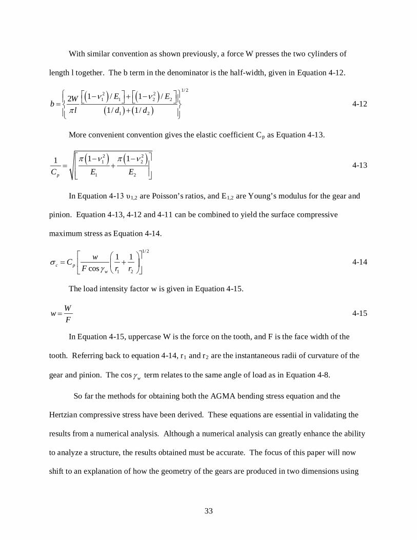
With similar convention as shown previously, a force W presses the two cylinders of
length l together. The b term in the denominator is the half-width, given in Equation 4-12.
( ) ( )( ) ( )
1/ 22 21 1 2 2
1 2
1 / 1 /21/ 1/
E EWbl d d
ν ν
π
− + − = + 4-12
More convenient convention gives the elastic coefficient Cp
( ) ( )2 21 2
1 2
1 11
pC E Eπ ν π ν − − = +
as Equation 4-13.
4-13
In Equation 4-13 υ1,2 are Poisson’s ratios, and E1,2
1/ 2
1 2
1 1cosc p
w
wCF r r
σγ
= +
are Young’s modulus for the gear and
pinion. Equation 4-13, 4-12 and 4-11 can be combined to yield the surface compressive
maximum stress as Equation 4-14.
4-14
The load intensity factor w is given in Equation 4-15.
WwF
= 4-15
In Equation 4-15, uppercase W is the force on the tooth, and F is the face width of the
tooth. Referring back to equation 4-14, r1 and r2
wγ
are the instantaneous radii of curvature of the
gear and pinion. The cos term relates to the same angle of load as in Equation 4-8.
So far the methods for obtaining both the AGMA bending stress equation and the
Hertzian compressive stress have been derived. These equations are essential in validating the
results from a numerical analysis. Although a numerical analysis can greatly enhance the ability
to analyze a structure, the results obtained must be accurate. The focus of this paper will now
shift to an explanation of how the geometry of the gears are produced in two dimensions using
34
ANSYS, how the boundary conditions and elements are chosen, and the method for obtaining an
accurate analysis and post-processing. Once this has been explained, the results will be
compared to the analytical results so that the justification and confidence of the results can be
verified.
Spur Gear Numerical Analysis Utilizing ANSYS
The first step to conduct a successful Finite Element Analysis is to create an accurate
geometry for the type of analysis you wish to consider. For this research, the structure of interest
is a spur gear and pinion meshing with each other. ANSYS Parametric Design Language
(APDL) is used to create the gear and pinion model, to apply contact and boundary conditions, to
control nonlinear solution sequence, and interpret analysis results. The code that was developed
for this problem is separated into four different files, each of which serves its own purpose in
creating the model, performing analysis, and interpreting the results.
The first file’s purpose is to provide the parameteric abilities of the gear design code.
Some parameters which are specific to gears are provided as input to the program. These
parameters are all of the necessary components which must be specified to completely generate a
gear and pinion.
Table 4-1 comprises the entirety of the first file. Its purpose is to provide these necessary
inputs to the second file which generates the actual geometries. A more detailed view of a spur
gear tooth is shown in Figure 4-7.
The modification of these parameters can yield a limitless combination of spur gear teeth.
This provides the design engineer with a powerful parametric tool capable of quickly adapting to
new designs.
The second file in the spur gear code serves to generate the 2 dimensional geometry of the
gear. One of the main components of this code is the ability to generate a parametrically
35
controlled involute curve to define the tooth shape. Involute curves can be thought of as follows.
First, pick a cylinder of any diameter, and place a piece of string tangent to a point on the
surface. While keeping the string taut, rotate the string around the radius of the cylinder. The
points traced by the end of the string will constitute an involute curve. Another definition of an
involute curve is given as, “any curve orthogonal to all the tangents to a given curve [43].”
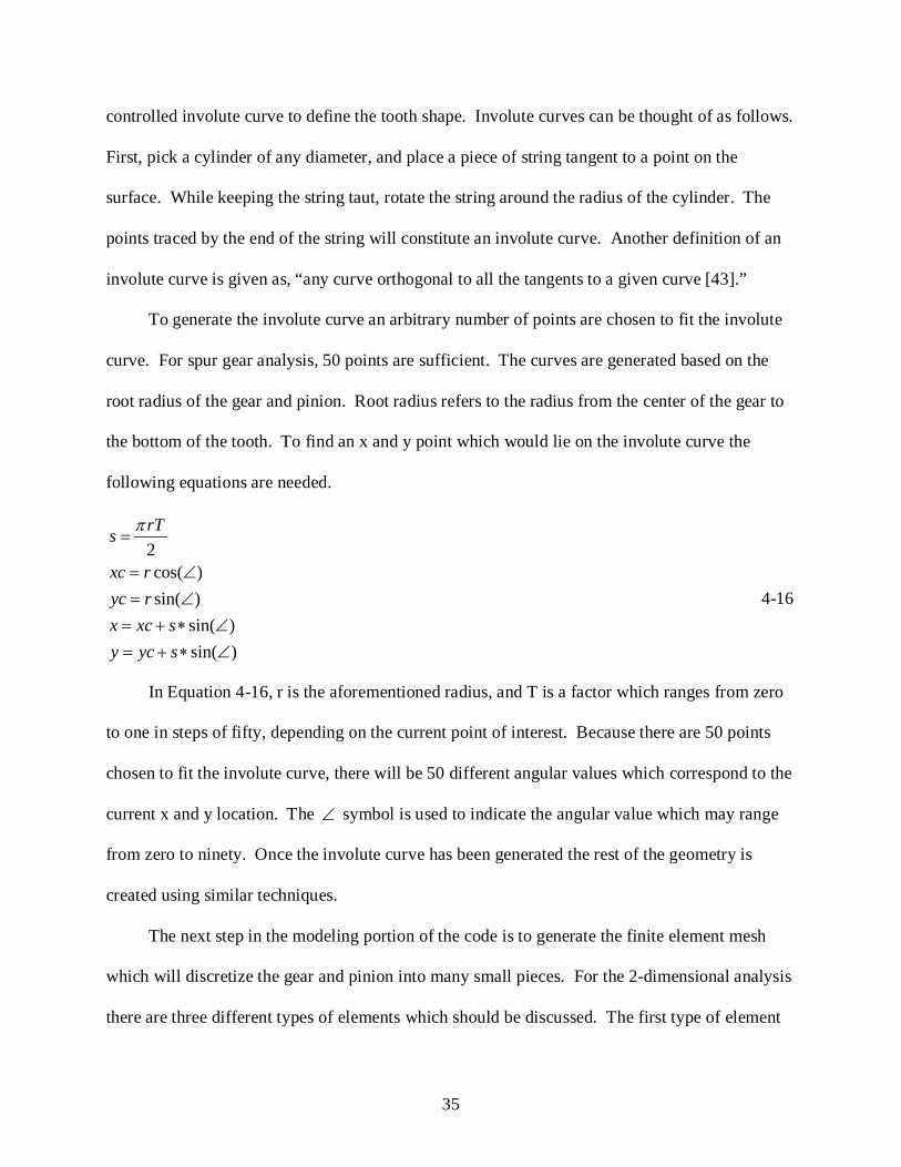
To generate the involute curve an arbitrary number of points are chosen to fit the involute
curve. For spur gear analysis, 50 points are sufficient. The curves are generated based on the
root radius of the gear and pinion. Root radius refers to the radius from the center of the gear to
the bottom of the tooth. To find an x and y point which would lie on the involute curve the
following equations are needed.
2cos( )sin( )
sin( )sin( )
rTs
xc ryc rx xc sy yc s
π=
= ∠= ∠= + ∗ ∠= + ∗ ∠
4-16
In Equation 4-16, r is the aforementioned radius, and T is a factor which ranges from zero
to one in steps of fifty, depending on the current point of interest. Because there are 50 points
chosen to fit the involute curve, there will be 50 different angular values which correspond to the
current x and y location. The ∠ symbol is used to indicate the angular value which may range
from zero to ninety. Once the involute curve has been generated the rest of the geometry is
created using similar techniques.
The next step in the modeling portion of the code is to generate the finite element mesh
which will discretize the gear and pinion into many small pieces. For the 2-dimensional analysis
there are three different types of elements which should be discussed. The first type of element
36
is a 4-node 2-dimensional element, referred to as PLANE182 in ANSYS APDL. This element
comprises the bulk of the gear and pinion area. This type of element incorporates finite strain
deformation with large rotation, based upon the principle of virtual work. Assumptions for the
use of this type of element are: strain is not infinitesimal, geometry changes during deformation,
to simulate nonlinear behavior incremental analysis is used and Cauchy stress is used with a
particular algorithm to take finite deformation into account. Although the equation for virtual
work, Cauchy stress, and displacement formulation are given, the discussion of their theory is
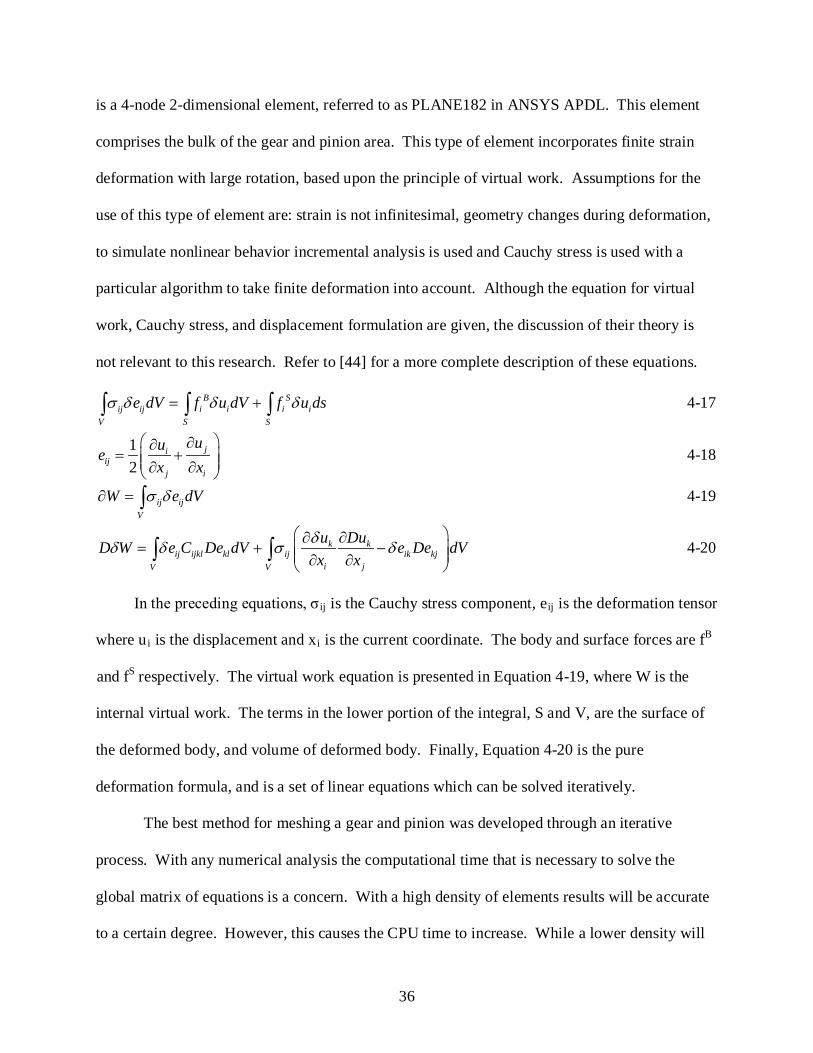
not relevant to this research. Refer to [44] for a more complete description of these equations.
B Sij ij i i i i
V S S
e dV f u dV f u dsσ δ δ δ= +∫ ∫ ∫ 4-17
12
jiij
j i
uuex x
∂∂= + ∂ ∂
4-18
ij ijV
W e dVσ δ∂ = ∫ 4-19
k kij ijkl kl ij ik kj
i jV V
u DuD W e C De dV e De dVx xδδ δ σ δ
∂ ∂= + − ∂ ∂ ∫ ∫ 4-20
In the preceding equations, σ ij is the Cauchy stress component, eij is the deformation tensor
where ui is the displacement and xi is the current coordinate. The body and surface forces are fB
and fS
The best method for meshing a gear and pinion was developed through an iterative
process. With any numerical analysis the computational time that is necessary to solve the
global matrix of equations is a concern. With a high density of elements results will be accurate
to a certain degree. However, this causes the CPU time to increase. While a lower density will
respectively. The virtual work equation is presented in Equation 4-19, where W is the
internal virtual work. The terms in the lower portion of the integral, S and V, are the surface of
the deformed body, and volume of deformed body. Finally, Equation 4-20 is the pure
deformation formula, and is a set of linear equations which can be solved iteratively.

37
yield quicker results, the accuracy is not guaranteed. There are a number of methods to modify
the mesh in order to achieve accurate results, with minimal computational effort. For this system
the area with the highest level of interest is the contact between the gear and pinion, as well as
the base of the teeth. To obtain accurate results it was necessary to increase the mesh density at
these points of interest. This capability has been programmed into the code to automatically
increase the mesh density near the regions of interest. This ensures accurate results with minimal
computation. Figure 4-8 illustrates the mesh necessary to obtain accurate results.
There are a few important aspects of this figure which should be mentioned. The first is
that away from the gear and pinion teeth the density of the mesh is much less than at the points
of contact and root of the teeth. The mesh density is much higher where contact occurs, but only
to a certain extent. Densely meshing the entire tooth is not necessary, only the line of contact is
meshed more densely. Also, the pinion (on the left) rotates counter-clockwise, meaning that
only the contact side of the teeth needs higher density meshing. Corresponding to this direction
of rotation is an intuitive understanding of where failure would be expected to occur based on
loading. Although the compressive stress at the base of the gear tooth may be higher than the
tensile stress, cracks will occur on the tensile side of the gear tooth, eventually leading to
catastrophic failure [45]. The authors of this study modeled a crack on the tensile side of the
gear tooth to predict remaining useful life. Therefore, it was only necessary to increase the mesh
density on this region of the gear tooth to provide accurate tensile stress results. The
combination of all of these factors led to the shortest possible computation time while still
providing accurate results.
38
The next type of element necessary to complete this analysis is known as a contact
element. The complement to this element is necessary as well, and is known as the target
element. The geometry of the contact and target elements are shown in Figure 4-9.
In Figure 4-9 the top surface is denoted as the “Target Surface”. This target surface is
defined by the geometry of the gear or pinion. As mentioned before the geometry of this section
was generated through a combination of an involute curve and then subsequently meshed with
the 2 dimensional plane stress elements. The “Target Element” is overlaid on the mesh already
created on the gear surface. The node numbering that was used for the 2 dimensional elements is
employed with the target element as well. Target elements will conform to the type of mesh
which is present on the surface of the geometry. This means that a target element could be either
one, two, or three nodes if midside nodes are used for the underlying surface. For this analysis, a
2 node target element is used to represent the contact between gear and pinion. For the entire
surface of the gear and pinion, target elements are generated to create a target surface.
The next region of interest is the “Contact Surface”. The contact surface corresponds to
the opposite surface from the target surface where contact is expected to occur. Similar to the
target element, the contact element conforms to the geometry and mesh type of the underlying
surface. Because the gear and pinion are similar, the contact element will also be a 2 node
element. The contact element is necessary to solve for the contact pressure and sliding distance
between the gear and pinion. ANSYS searches for contact between the target and contact
surfaces, and contact must always occur in the normal direction. It is necessary to input the type
of stress state for this element, which is plane stress. In addition to inputting plane stress, the
thickness of the gear is input so that results are consistent. In Figure 4-9 notice that the contact
element and target element are not necessarily contacting at the nodal locations. Contact is
39
calculated at integration points located within each element, and then averaged across the
element surface. The contact element is a non-linear element, and requires full iterative Newton
solutions. Because of this, computational time can be significant depending on the number of
contact elements which are present.
The previous explanation shows how a contact set would be applied between a gear and
pinion. However, because there is only one target surface and one contact surface, results would
only be given on the contact surface. To remedy this situation, the opposite formulation is
necessary to obtain results on both surfaces. This is achieved by creating a target surface where
the contact surface was present in Figure 4-9, and a contact surface where the target surface was.
By this procedure results for the contact pressure can be obtained for both gear and pinion. Now
that the gear and pinion have been meshed with both solid elements and contact elements, results
for both bending stress and contact stress will be available.
The next step in the modeling process is to begin applying boundary conditions and
necessary restrictions to ensure that the results obtained are accurate. The first step in applying
these boundary conditions is to generate an additional set of elements known as “rigid elements”.
The purpose of these rigid elements is to apply kinematic constraints between nodes. These
elements are necessary to properly constrain the rotations of the gear and pinion. The specific
type of element is known as a rigid beam, and the direct elimination method is used to apply the
constraints. The direct elimination method is imposed by internally generated multipoint
constraint equations [46]. Nodes are created at the center of rotation for both the gear and
pinion. This node is constrained in all six degrees of freedom, and the rigid beam elements are
connected between this node and the inside diameter of the gear and pinion. The final step in the
modeling process is to copy the area of the pinion in minute increments until contact occurs with
40
the gear. This is done iteratively until contact just occurs, and then the process is stopped. At
this point, the finite element solution is ready to begin.
The simulation phase of the finite element gear program is divided into two parts. The first
section of the code is responsible for first ensuring that the non linear geometry option is
selected. Then, a torque is applied to the pinion around the z-axis. Recall that contact has
already been established between the gear and the pinion. Ramp loading is used to gradually
apply this torque while the gear is held in place. Once this solution has converged for the
prescribed number of sub-steps, the next section of the solution code is run. For this portion, the
rotation of the gear about the z-axis is prescribed. The applied torque from the previous load
step is held constant at the prescribed value. Because only a portion of the gear is being
modeled, the rotation is confined to 2Nπ where N is the number of teeth of the gear. This
rotation is broken up into 40 sub-steps which solve the non-linear contact equations at each step.
Based on the geometry and mesh shown this solution phase generally takes around 90 minutes of
CPU time to complete. Once the solution is complete, the post-processing of the data may
commence.
The post-processing of the data is straight forward for bending stress and contact pressure
calculations. For the bending stress it was mentioned previously that the region where tensile
stress is present is the region of interest. The node at which the maximum value is achieved
throughout the solution process is noted, and the data for each sub-step recorded. Next, for the
contact pressure the same type of analysis is performed. The critical node is chosen and its
contact pressure values throughout the analysis are recorded. The only difference with the
contact pressure calculation involves the scarcity of data. Contact may only occur for one or two
sub-steps in the entire 40 sub-step process. Therefore, the Von Mises contact stress is also
41
recorded at the node of interest. When the contact is actually occurring, the values for contact
pressure and Von Mises stress will closely correspond. Figure 4-10 presents a schematic of the
FEA code, and the following sub-chapter will compare the numerical to the analytical results.
Comparison of Numerical to Analytical Results
The first step in comparing the numerical to analytical results was choosing a valid gear for
the analysis. One reference in the gearing community was chosen, and was able to provide
relevant data for a typical gear [47]. Based upon recommendations, an input torque of 800 N-m
was applied to the pinion. The corresponding calculations from the parameters given in Table 4-
1 are shown in Figure 4-11. This spreadsheet contains the relevant equations discussed
previously.
Figure 4-11 provides all of the necessary information to predict both the contact pressure and
maximum bending stress in accordance with the AGMA guidelines. The first parameter column
mainly lists the values given in Table 4-1. Judicious decisions are necessary to properly
determine whether parameters from the gear or pinion should be used. In all cases, the value
which would provide a higher stress or contact pressure are utilized. The remaining columns are
based on AGMA calculations that were given in previous sections. These are mostly geometric
properties specific to this particular gear. Whenever a new or different gear is introduced, one
must manually input the parameters of column one to generate results. Also, in the final column
of Figure 4-11 x and y values of 34.45 and 3.71 mms are given. These values were chosen to
maximize the final result for σ t. The x and y values must correspond to real values which are
present at the base of the pinion. Values which lie outside of the gear volume are invalid. The
process of maximizing the x and y values can vary depending on the software used. Microsoft
Excel has an embedded feature which allows the user to maximize an equation based on given
constraints. This was the method chosen for this research. From Figure 4-11 the highlighted
42
values for σc and σ t
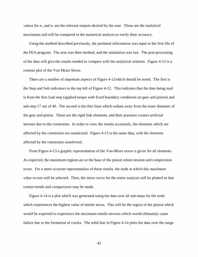
Figure 4-14
are the relevant outputs desired by the user. These are the analytical
maximums and will be compared to the numerical analysis to verify their accuracy.
Using the method described previously, the pertinent information was input to the first file of
the FEA program. The area was then meshed, and the simulation was run. The post-processing
of the data will give the results needed to compare with the analytical solution. Figure 4-12 is a
contour plot of the Von Mises Stress.
There are a number of important aspects of Figure 4-12which should be noted. The first is
the Step and Sub indicators in the top left of Figure 4-12. This indicates that the data being read
is from the first load step (applied torque with fixed boundary conditions on gear and pinion) and
sub-step 17 out of 40. The second is the thin lines which radiate away from the inner diameter of
the gear and pinion. These are the rigid link elements, and their presence creates artificial
stresses due to the constraints. In order to view the results accurately, the elements which are
affected by the constraints are unselected. Figure 4-13 is the same data, with the elements
affected by the constraints unselected.
From Figure 4-13 a graphic representation of the Von-Mises stress is given for all elements.
As expected, the maximum regions are at the base of the pinion where tension and compression
occur. For a more accurate representation of these results, the node at which this maximum
value occurs will be selected. Then, the stress curve for the entire analysis will be plotted so that
certain trends and comparisons may be made.
is a plot which was generated using the data over all sub-steps for the node
which experiences the highest value of tensile stress. This will be the region of the pinion which
would be expected to experience the maximum tensile stresses which would ultimately cause
failure due to the formation of cracks. The solid line in Figure 4-14 plots the data over the range
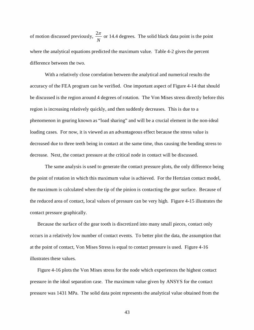
43
of motion discussed previously, 2Nπ or 14.4 degrees. The solid black data point is the point
where the analytical equations predicted the maximum value. Table 4-2 gives the percent
difference between the two.
With a relatively close correlation between the analytical and numerical results the
accuracy of the FEA program can be verified. One important aspect of Figure 4-14 that should
be discussed is the region around 4 degrees of rotation. The Von Mises stress directly before this
region is increasing relatively quickly, and then suddenly decreases. This is due to a
phenomenon in gearing known as “load sharing” and will be a crucial element in the non-ideal
loading cases. For now, it is viewed as an advantageous effect because the stress value is
decreased due to three teeth being in contact at the same time, thus causing the bending stress to
decrease. Next, the contact pressure at the critical node in contact will be discussed.
The same analysis is used to generate the contact pressure plots, the only difference being
the point of rotation in which this maximum value is achieved. For the Hertzian contact model,
the maximum is calculated when the tip of the pinion is contacting the gear surface. Because of
the reduced area of contact, local values of pressure can be very high. Figure 4-15 illustrates the
contact pressure graphically.
Because the surface of the gear tooth is discretized into many small pieces, contact only
occurs in a relatively low number of contact events. To better plot the data, the assumption that
at the point of contact, Von Mises Stress is equal to contact pressure is used. Figure 4-16
illustrates these values.
Figure 4-16 plots the Von Mises stress for the node which experiences the highest contact
pressure in the ideal separation case. The maximum value given by ANSYS for the contact
pressure was 1431 MPa. The solid data point represents the analytical value obtained from the
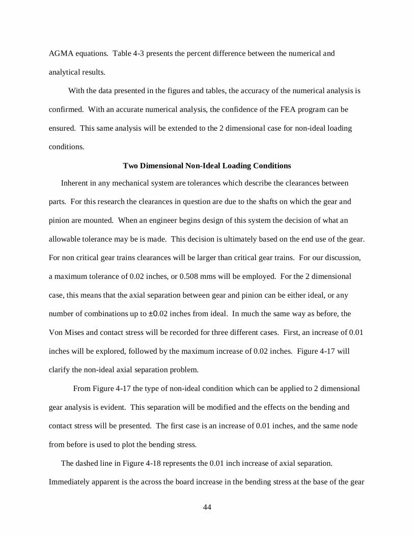
44
AGMA equations. Table 4-3 presents the percent difference between the numerical and
analytical results.
With the data presented in the figures and tables, the accuracy of the numerical analysis is
confirmed. With an accurate numerical analysis, the confidence of the FEA program can be
ensured. This same analysis will be extended to the 2 dimensional case for non-ideal loading
conditions.
Two Dimensional Non-Ideal Loading Conditions
Inherent in any mechanical system are tolerances which describe the clearances between
parts. For this research the clearances in question are due to the shafts on which the gear and
pinion are mounted. When an engineer begins design of this system the decision of what an
allowable tolerance may be is made. This decision is ultimately based on the end use of the gear.
For non critical gear trains clearances will be larger than critical gear trains. For our discussion,
a maximum tolerance of 0.02 inches, or 0.508 mms will be employed. For the 2 dimensional
case, this means that the axial separation between gear and pinion can be either ideal, or any
number of combinations up to ±0.02 inches from ideal. In much the same way as before, the
Von Mises and contact stress will be recorded for three different cases. First, an increase of 0.01
inches will be explored, followed by the maximum increase of 0.02 inches. Figure 4-17 will
clarify the non-ideal axial separation problem.
From Figure 4-17 the type of non-ideal condition which can be applied to 2 dimensional
gear analysis is evident. This separation will be modified and the effects on the bending and
contact stress will be presented. The first case is an increase of 0.01 inches, and the same node
from before is used to plot the bending stress.
The dashed line in Figure 4-18 represents the 0.01 inch increase of axial separation.
Immediately apparent is the across the board increase in the bending stress at the base of the gear
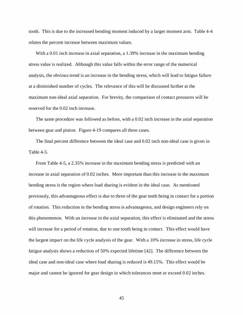
45
tooth. This is due to the increased bending moment induced by a larger moment arm. Table 4-4
relates the percent increase between maximum values.
With a 0.01 inch increase in axial separation, a 1.39% increase in the maximum bending
stress value is realized. Although this value falls within the error range of the numerical
analysis, the obvious trend is an increase in the bending stress, which will lead to fatigue failure
at a diminished number of cycles. The relevance of this will be discussed further at the
maximum non-ideal axial separation. For brevity, the comparison of contact pressures will be
reserved for the 0.02 inch increase.
The same procedure was followed as before, with a 0.02 inch increase in the axial separation
between gear and pinion. Figure 4-19 compares all three cases.
The final percent difference between the ideal case and 0.02 inch non-ideal case is given in
Table 4-5.
From Table 4-5, a 2.35% increase in the maximum bending stress is predicted with an
increase in axial separation of 0.02 inches. More important than this increase in the maximum
bending stress is the region where load sharing is evident in the ideal case. As mentioned
previously, this advantageous effect is due to three of the gear teeth being in contact for a portion
of rotation. This reduction in the bending stress is advantageous, and design engineers rely on
this phenomenon. With an increase in the axial separation, this effect is eliminated and the stress
will increase for a period of rotation, due to one tooth being in contact. This effect would have
the largest impact on the life cycle analysis of the gear. With a 10% increase in stress, life cycle
fatigue analysis shows a reduction of 50% expected lifetime [42]. The difference between the
ideal case and non-ideal case where load sharing is reduced is 49.15%. This effect would be
major and cannot be ignored for gear design in which tolerances meet or exceed 0.02 inches.
46
Next, the Von Mises stress at the point of contact is given for the same node as was
previously recorded.
Figure 4-20 is a plot of the Von Mises Stress for a node near the tip of the pinion. When
an ideal separation between gear and pinion exists, the maximum value obtained from ANSYS
was 1431 MPa. With a 0.02 inch increase in the separation between gear and pinion, the contact
pressure can be as large as 1648 MPa.
In Figure 4-20, keep in mind that the axial separation between gear and pinion has increased.
Due to this change in separation, the point of contact is no longer the same as the ideal case.
This is the reason why the dashed plot shows contact occurring at an earlier angular rotation than
the ideal case. Due to the axial separation increase of 0.02 inches, the contact pressure can
increase by as much as 15%. This would undoubtedly lead to higher rates of wear and fatigue.
Thus far the method to simulate a 2 dimensional gear subject to increases in axial
separation has been presented. The next section will present the 3 dimensional case, and the
non-ideal conditions that may arise.
Three Dimensional Non-Ideal Loading Condtions
The method of producing a 3 dimensional volume in ANSYS is similar to the 2 dimensional
method. The same file is used to first generate the 2 dimensional area which is identical to the
gear and pinion used in the previous sub-chapter. Then, the area can be extruded to produce a 3
dimensional volume. Instead of using 2 dimensional plane stress elements, the element type is
modified to represent the new 3 dimensional geometry. For the area mesh of the gear and
pinion, the plane stress 4 node element was used. Commands in ANSYS are issued to extrude
the area to generate a volume. This will create 8 node brick elements for the bulk material,
known as SOLID45 in ANSYS. In addition to solid elements, the contact elements for 3
dimensional analysis must be modified as well. For the target elements, TARGE170 is the
47
preferred element for 3 dimensional analysis. This element can be used to represent any number
of geometries, corresponding to the underlying structure. Because the 8 node brick element is
the underlying structure, 4 node quadrilateral target elements are generated. Similar to the 2
dimensional analysis, generation of contact elements on the converse surface is necessary as
well. CONTA173 elements are used in ANSYS, which are 3 dimensional 4 node contact
elements. This element conforms to the underlying geometry of the associated surface, and is
overlaid on the SOLID45 elements. Also, it is necessary to create contact and target elements on
both the gear and pinion so that results are available for each.
Figure 4-21 presents the 3 dimensional gear and pinion which will be used for this analysis.
Next, two additional non-ideal loading conditions will be presented.
Figure 4-21 represents the 3 dimensional model assembled under optimal conditions. The
results from this analysis will be compared to combinations of the following non-ideal cases: out
of plane translation and b-axis rotation. The increased axial separation case has been discussed
previously and the results are similar. The corresponding representations will be followed by a
brief description to completely describe the type of non-ideal condition.
Figure 4-22 presents the first two non-ideal loading conditions. The figure labeled “front
view” relates the increased axial separation discussed previously. The “top view” relates the out
of plane translation. The offset shown above is 0.02 inches, similar to the maximum axial
separation. Figure 4-23 gives the b-axis rotation, which is the notation in the industry for
rotation about the y-axis. The following will help to clarify this situation.
Figure 4-23 is a highly exaggerated case for the final non-ideal loading condition. The b-axis
rotation corresponds to a rotation about the y-axis, and a value of 5 degrees is shown in Figure 4-
23 so that the b-axis rotation can be seen clearly. For this research, the maximum b-axis rotation
48
is taken to be 0.5 degrees. Next, the results for both the ideal and non-ideal loading cases will be
presented.
First, the results for the ideal 3 dimensional spur gear are given. For the 3 dimensional case,
a number of important modifications have been made. The first is the size of the gear. In the 2
dimensional case, the face width of the gear is 31.75 mm. For lower computational time, this
was modified to 1.25 mm. For a gear whose face width has been reduced to such a small degree,
the load must be reduced as well. The torque was changed to 5 Nm to compensate for the
reduction in face width. Finally, the method used to compare the results will be modified as
well. Along the base of the gear tooth, 6 nodes are chosen and the Von Mises stress recorded at
each sub-step. The maximum of these values will be compared for each case to determine the
response. The contact stress will be plotted as before. Table 4-7 gives the node number and
stress values for the nodes at the base of the gear tooth.
Table 4-7 is the bending stress data recorded at the base of the gear. These values were chosen
during the load step where the maximum bending stress occurs. This data will be compared to
the cases for the out of plane translation, and the rotation in the b-axis. Figure 4-24 gives the
contact stress for the node which experiences the maximum value.
Figure 4-24 is a plot of the contact stress for the node which experiences the maximum
value for the ideal case. The maximum contact stress value is 85.28 MPa and occurs at about
11.5 degrees of rotation. The next case will be the out of plane translation.
Because the width of the gear has been reduced by a large amount, the amount of
expected out of plane translation must decrease as well. For this research the maximum out of
plane translation was reduced to 0.25 mm. Table 4-8 gives the comparison to the ideal case for
the bending stress values.
49
Table 4-8 compares the bending stress for the same nodes for both the ideal and non-ideal
case. For each node an increase in the bending stress is noted, with a maximum increase of
45.75%. The ideal vs. non-ideal contact stress is presented in Figure 4-25.
Figure 4-25 presents the ideal contact stress vs. the out of plane contact stress. This data
is plotted for the same node as before, and contact occurs during the same rotational angles.
With an out of plane translation the contact stress increases from 85.28 MPa to 130.35 MPa, a
difference of 52.8%. The reason the contact pressure increases can be explained because of the
smaller area of contact. In effect, providing an out of plane translation is reducing the area of
contact while keeping the same torque constant. This reduction in contact area will cause the
contact stress to increase. The final non-ideal case will compare the ideal bending and contact to
a rotation about the b-axis.
Table 4-9 presents the data for the ideal vs. the non-ideal case. For all nodes a reduction in
the bending stress is noted, with the maximum reduction of 50.08%. Finally, the comparison of
the ideal contact stress vs. b-axis rotation is given.
Figure 4-26 presents both the ideal contact stress and b-axis rotational contact stress. As
before, the ideal stress is 85.28 MPa, and the non-ideal case is 144.24 MPa. This is a percent
difference of 69.13%. When the b-axis rotation is introduced, the line of contact between gear
and pinion is disrupted. Because ideal contact conditions no longer exist, the contact stress will
increase.
The trend of non-ideal conditions on the response of the spur gear is consistent. With out
of plane translations and b-axis rotations, the bending stress increases in the first case, and
decreases in the latter. Due to these modifications of the stress values, the predicted lifetime of
the spur gear will be modified. In addition to the bending stress, the contact stress increases for
50
each non-ideal case as well. With an increase in the contact stress, Archard’s wear model will
predict higher levels of wear depth. This phenomenon will be presented in the case where non-
ideal wear is presented.
Archard’s Wear Model for Gear Wear
The analysis up to this point has focused on the response of both the bending and contact
stress of a gear and pinion due to the introduction of certain non-ideal loading conditions. The
remaining focus will now center on predicting progressive wear evolution using ANSYS.
Progressive wear evolution is the combination of predicting a certain wear depth based on
a set extrapolation scheme, modifying the nodal locations based on contact pressure, sliding
distance, and a wear constant, and finally rerunning the simulation based on these new nodal
locations. In this manner, the influence of past wear on current wear is included.
Archard’s wear model is based on the assumption that the wear volume due to abrasive
wear is given as:
NFV Ks H= 4-21
In Equation 4-21, V is the worn volume, s is the sliding distance, K is the wear constant,
non-dimensional in Equation 4-21, FN
V h KPsA sdh KPds
= =
=
is the normal load, and H is the hardness of the material
[19,48]. For a more convenient notation, the wear depth is given as Equation 4-22.
or h KPs= 4-22
By dividing through by the area A, the volume divided by area leaves height h. Then, the
wear progress can be described by a differential equation with its prediction as an initial value
51
problem [49]. In Equation 4-22, K has the units of 3mm
Nm From ANSYS, the contact pressure
and sliding distance are both degrees of freedom for the selected node, and thus their data is
readily obtained. The next topic of concern is picking a valid wear constant value. To do this, a
number of experimental papers will be referenced. An experimental study conducted by Walton
and Goodwin [50] noted wear constants from 2.4×10⁻⁵ to 9.3×10⁻⁸ where the wear constant is
non-dimensional. These values were experimentally studied for spur gears subject to non-
lubricated sliding. Other studies have found experimental values as low as 1×10-11 for the wear
rate of lubricated spur gears [51]. Thus, careful consideration must be taken into account when
choosing a valid wear constant.
Once the wear depth is calculated in ANSYS, the direction in which to update the wear
depth is crucial. Because the nodal locations are being modified, each node will have a unique
direction for update. Because the contact pressure is assumed to be normal to the surface, the
nodal locations will also be updated normal to the surface. Figure 4-27 shows the typical
arrangement of nodes on the surface of a gear tooth.
From Figure 4-27, an arbitrary node is located at position x,y. Its neighboring nodes are
located at positions xn+1,yn+1 and xn-1,yn-1
1 1
1 1
x n n
y n n
d x xd y y
+ −
+ −
= −= −
. The desired normal direction is N. Then, the
difference between these coordinates is given by Equation 4-23.
4-23
In Equation 4-23 dx and dy are the difference in location between node n+1 and node n-1.
Then, the normal direction can be computed via Equation 4-24.
52
2 2
ˆˆˆˆ 0
0 0 1
ˆˆ(̂ ) ( ) 0ˆˆ
i j kN d k dx dy
i dy j dx kdyi dxjNdx dy
= × =
= − +
−=
+
4-24
In Equation 4-24, the normal direction N is the cross product of the d vector and unit
vector k, in the positive z-direction. The cross product divided by the magnitude then yields the
normal direction. The nodal locations will then be updated by the product of the normal
direction N, and the wear depth h.
The next step in the calculation of wear depth and geometry update for the spur gear
problem is to decide on a value of the wear constant. For this research where un-lubricated
sliding of spur gears is considered, a value of 3×10-83mm
Nm is used. The final step before results
of the wear analysis are presented involves the hierarchal scheme used in ANSYS to solve the
wear problem, while still extrapolating to reduce computational time. Figure 4-28 will be
presented to give the reader the understanding of how the wear program is included in the
previously presented FEA program.
In Figure 4-28 the same files are present as in the previous explanation. The addition of an
extra file which does the wear depth calculations and geometry update is the only new addition.
This file is embedded within the analysis section of the FEA code. The prescribed number of
cycles can be input to the simulation code, and the wear code will run until that number of cycles
has been completed.
Thus far, the FEA code and the results shown are from one complete cycle of the gear and
pinion. For the wear code it is necessary to run multiple cycles in order to predict wear and the
53
evolution of this wear. Therefore, 20 wear cycles were chosen with an extrapolation of 3,000
cycles per analysis. This results in a total number of gear cycles of 60,000 over the course of 20
FEA simulations. From writing and experimenting with the FEA code 60,000 revolutions of the
gear was the maximum number attainable without re-meshing. When more revolutions and wear
cycles were attempted, the FEA solver diverges because of excessive element distortion.
To best illustrate the wear results a number of plots will be generated. All nodes along
the exterior of the pinion were selected, and their corresponding wear depth recorded. The plots
will be presented with the node number on the x-axis, and the wear depth in mm on the y-axis.
This first plot shows incremental wear from the first cycle and the last cycle. This is not the total
accumulated wear, but illustrates how the progressive wear evolves from cycle 1 to cycle 60,000.
Figure 4-29 presents the data for the first and last wear cycle for the middle tooth of the
pinion. The first cycle, shown as the solid line, has a maximum nodal wear depth of about 2×10-
4
From Figure 4-30 the oscillations seen in the incremental wear depths have diminished.
The maximum wear depth for 60,000 cycles is predicted to be about 3×10
mm. As this would represent a valley in the surface of the pinion, less contact would occur at
this point until the surrounding area’s surface is worn away. This is the reason that the final
cycle has less wear depth in this region. Also, for the first cycle there is an oscillation in the
wear depths seen from node 1677 to node 1687. As the wear progresses, the final wear cycle
indicated by the dashed line is deeper at points in which the solid line are shallower. This further
indicates the evolution of progressive wear. One final comment on Figure 4-29 is the area of
relatively little wear for both the first and last cycle. This will be explained with a corresponding
plot of the sliding distance between gear and pinion, but for now the total accumulated wear
depth for 60,000 cycles is given in Figure 4-30.
-3 mm, with the same
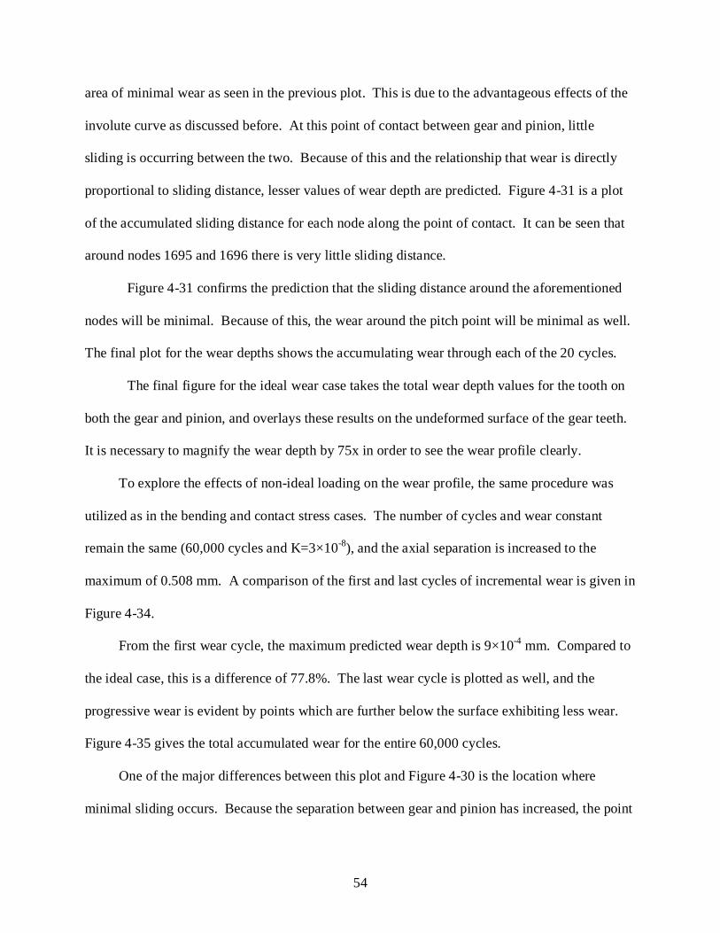
54
area of minimal wear as seen in the previous plot. This is due to the advantageous effects of the
involute curve as discussed before. At this point of contact between gear and pinion, little
sliding is occurring between the two. Because of this and the relationship that wear is directly
proportional to sliding distance, lesser values of wear depth are predicted. Figure 4-31 is a plot
of the accumulated sliding distance for each node along the point of contact. It can be seen that
around nodes 1695 and 1696 there is very little sliding distance.
Figure 4-31 confirms the prediction that the sliding distance around the aforementioned
nodes will be minimal. Because of this, the wear around the pitch point will be minimal as well.
The final plot for the wear depths shows the accumulating wear through each of the 20 cycles.
The final figure for the ideal wear case takes the total wear depth values for the tooth on
both the gear and pinion, and overlays these results on the undeformed surface of the gear teeth.
It is necessary to magnify the wear depth by 75x in order to see the wear profile clearly.
To explore the effects of non-ideal loading on the wear profile, the same procedure was
utilized as in the bending and contact stress cases. The number of cycles and wear constant
remain the same (60,000 cycles and K=3×10⁻⁸), and the axial separation is increased to the
maximum of 0.508 mm. A comparison of the first and last cycles of incremental wear is given in
Figure 4-34.
From the first wear cycle, the maximum predicted wear depth is 9×10⁻⁴
One of the major differences between this plot and
mm. Compared to
the ideal case, this is a difference of 77.8%. The last wear cycle is plotted as well, and the
progressive wear is evident by points which are further below the surface exhibiting less wear.
Figure 4-35 gives the total accumulated wear for the entire 60,000 cycles.
Figure 4-30 is the location where
minimal sliding occurs. Because the separation between gear and pinion has increased, the point
55
at which the gears transmit their power is modified. When this point of contact is modified, ideal
power transmission will not be realized. In turn, this causes the wear between gear and pinion to
increase. In addition to the point of minimal sliding being modified, the bending stress increases
as well. Thus there will be more wear near the base of the tooth with an increased value for the
bending stress. Table 4-10 gives the percent differences between the ideal and non-ideal case.
From Table 4-10 the maximum wear depth increased 22.59% with an increase of 0.508
mm axial separation.
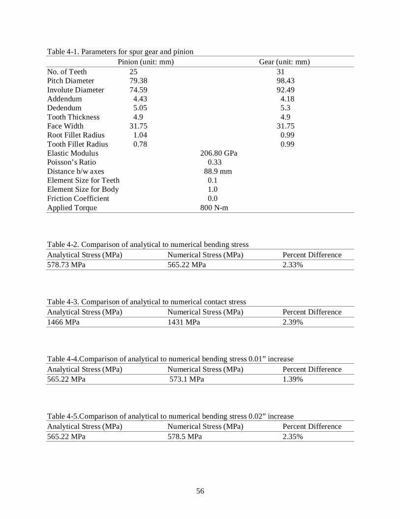
56
Table 4-1. Parameters for spur gear and pinion Pinion (unit: mm) Gear (unit: mm) No. of Teeth 25 31 Pitch Diameter 79.38 98.43 Involute Diameter 74.59 92.49 Addendum 4.43 4.18 Dedendum 5.05 5.3 Tooth Thickness 4.9 4.9 Face Width 31.75 31.75 Root Fillet Radius 1.04 0.99 Tooth Fillet Radius 0.78 0.99 Elastic Modulus 206.80 GPa Poisson’s Ratio 0.33 Distance b/w axes 88.9 mm Element Size for Teeth 0.1 Element Size for Body 1.0 Friction Coefficient 0.0 Applied Torque 800 N-m Table 4-2. Comparison of analytical to numerical bending stress Analytical Stress (MPa) Numerical Stress (MPa) Percent Difference 578.73 MPa 565.22 MPa 2.33% Table 4-3. Comparison of analytical to numerical contact stress Analytical Stress (MPa) Numerical Stress (MPa) Percent Difference 1466 MPa 1431 MPa 2.39% Table 4-4.Comparison of analytical to numerical bending stress 0.01” increase Analytical Stress (MPa) Numerical Stress (MPa) Percent Difference 565.22 MPa 573.1 MPa 1.39% Table 4-5.Comparison of analytical to numerical bending stress 0.02” increase Analytical Stress (MPa) Numerical Stress (MPa) Percent Difference 565.22 MPa 578.5 MPa 2.35%
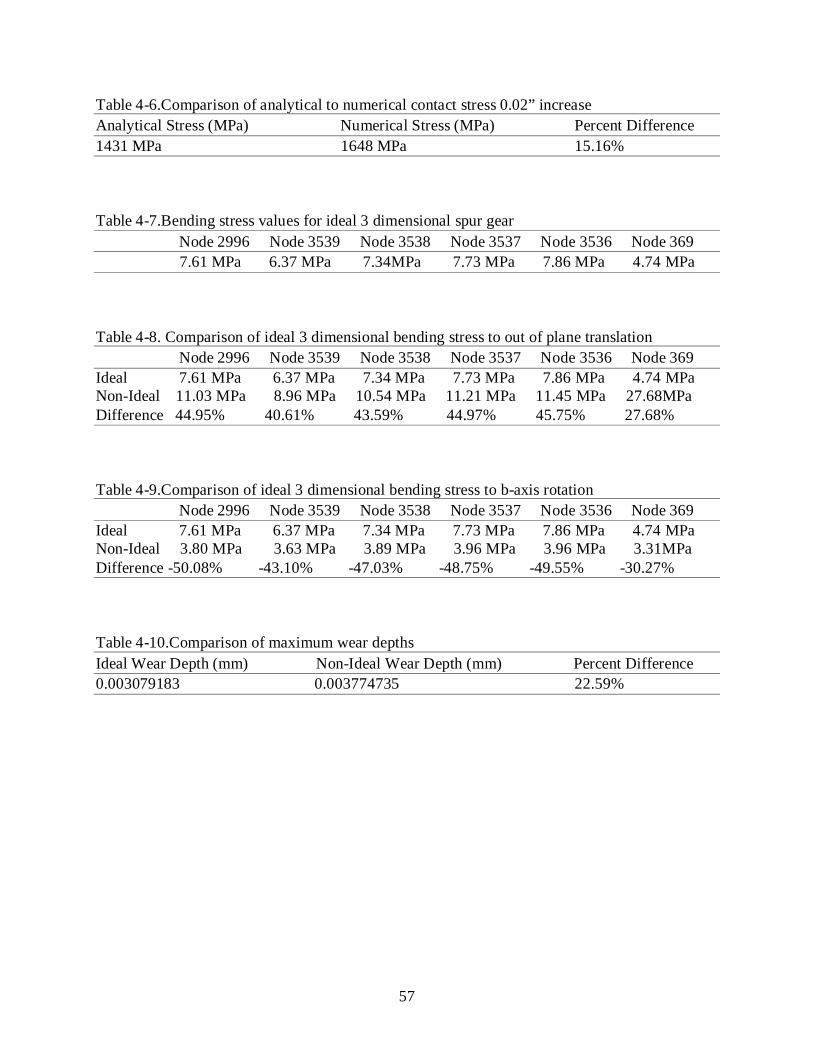
57
Table 4-6.Comparison of analytical to numerical contact stress 0.02” increase Analytical Stress (MPa) Numerical Stress (MPa) Percent Difference 1431 MPa 1648 MPa 15.16% Table 4-7.Bending stress values for ideal 3 dimensional spur gear Node 2996 Node 3539 Node 3538 Node 3537 Node 3536 Node 369 7.61 MPa 6.37 MPa 7.34MPa 7.73 MPa 7.86 MPa 4.74 MPa Table 4-8. Comparison of ideal 3 dimensional bending stress to out of plane translation Node 2996 Node 3539 Node 3538 Node 3537 Node 3536 Node 369 Ideal 7.61 MPa 6.37 MPa 7.34 MPa 7.73 MPa 7.86 MPa 4.74 MPa Non-Ideal 11.03 MPa 8.96 MPa 10.54 MPa 11.21 MPa 11.45 MPa 27.68MPa Difference 44.95% 40.61% 43.59% 44.97% 45.75% 27.68%
Table 4-9.Comparison of ideal 3 dimensional bending stress to b-axis rotation Node 2996 Node 3539 Node 3538 Node 3537 Node 3536 Node 369 Ideal 7.61 MPa 6.37 MPa 7.34 MPa 7.73 MPa 7.86 MPa 4.74 MPa Non-Ideal 3.80 MPa 3.63 MPa 3.89 MPa 3.96 MPa 3.96 MPa 3.31MPa Difference -50.08% -43.10% -47.03% -48.75% -49.55% -30.27% Table 4-10.Comparison of maximum wear depths Ideal Wear Depth (mm) Non-Ideal Wear Depth (mm) Percent Difference 0.003079183 0.003774735 22.59%
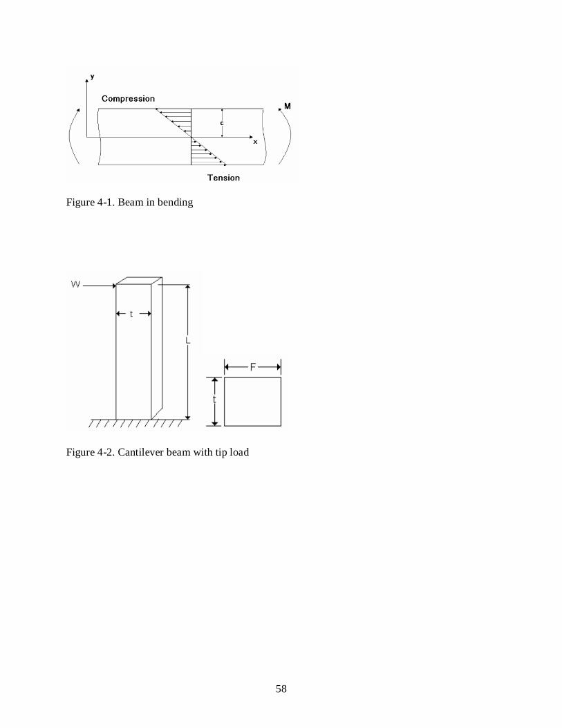
58
Figure 4-1. Beam in bending
Figure 4-2. Cantilever beam with tip load
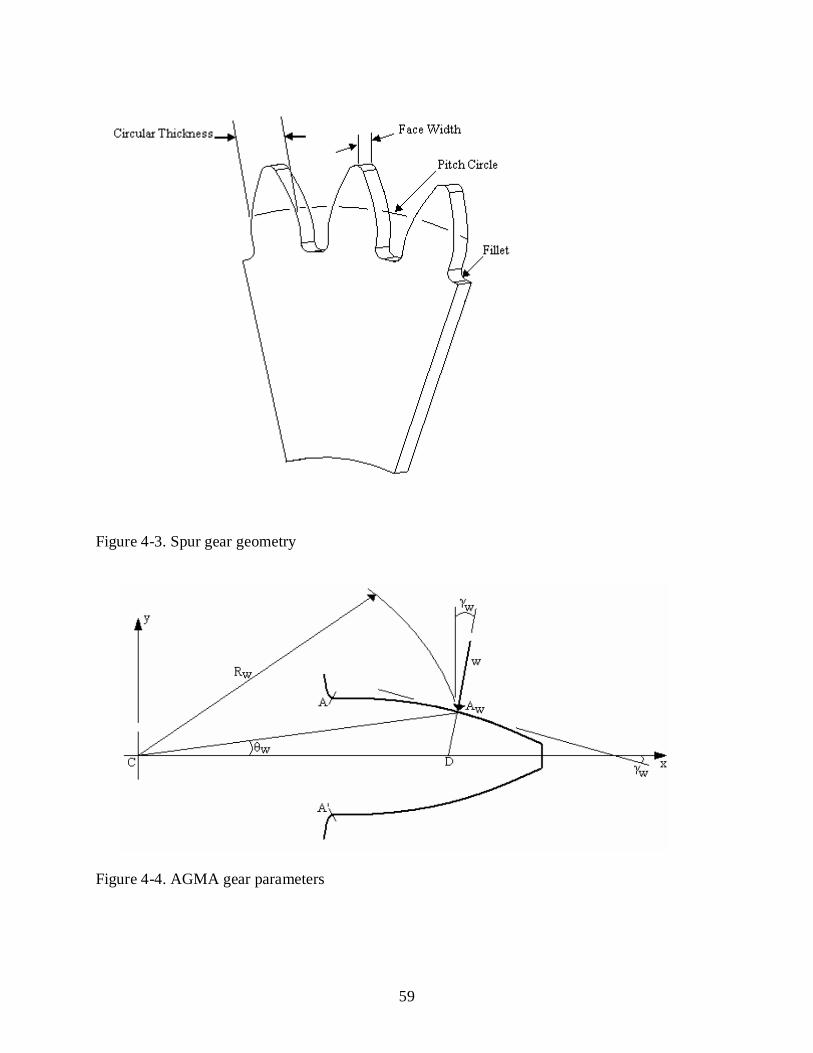
59
Figure 4-3. Spur gear geometry
Figure 4-4. AGMA gear parameters
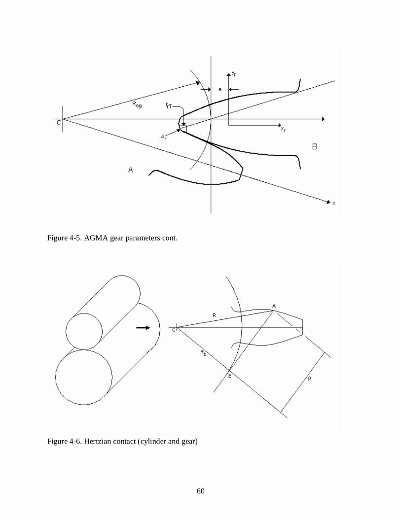
60
Figure 4-5. AGMA gear parameters cont.
Figure 4-6. Hertzian contact (cylinder and gear)
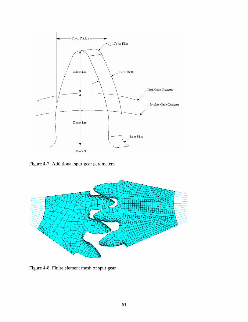
61
Figure 4-7. Additional spur gear parameters
Figure 4-8. Finite element mesh of spur gear
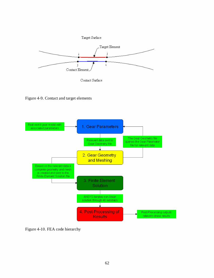
62
Figure 4-9. Contact and target elements
Figure 4-10. FEA code hierarchy
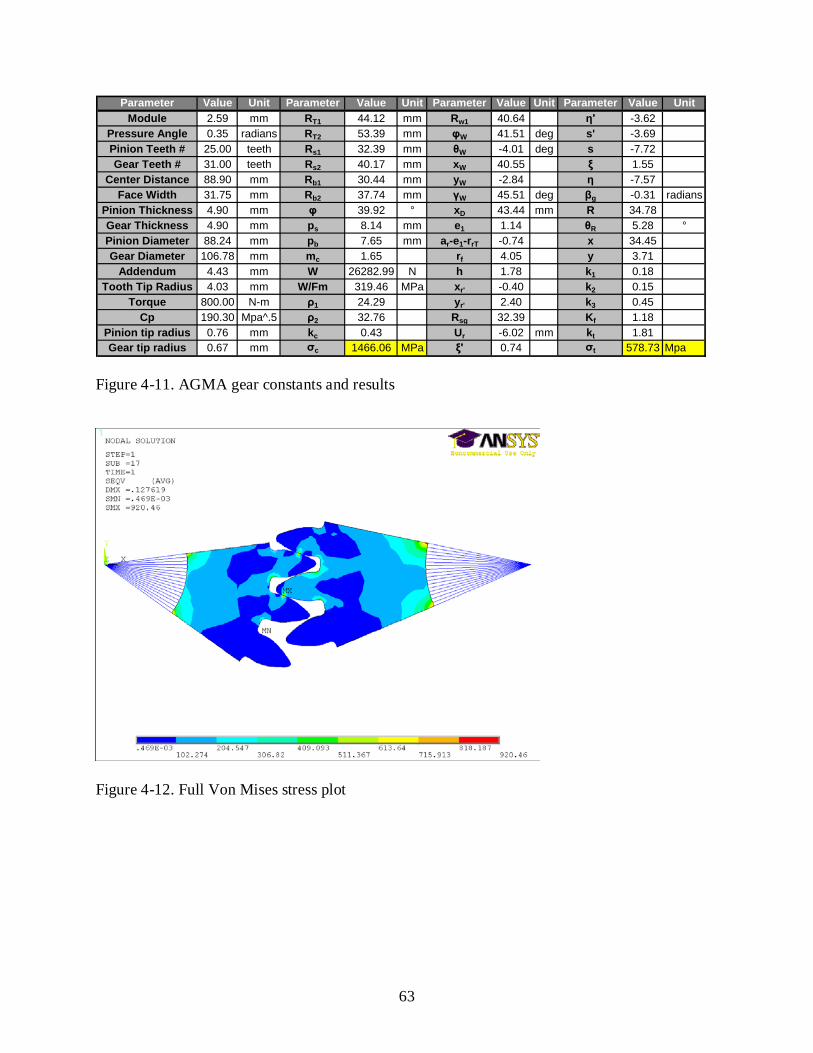
63
Parameter Value Unit Parameter Value Unit Parameter Value Unit Parameter Value UnitModule 2.59 mm RT1 44.12 mm Rw1 40.64 η' -3.62
Pressure Angle 0.35 radians RT2 53.39 mm φW 41.51 deg s' -3.69Pinion Teeth # 25.00 teeth Rs1 32.39 mm θW -4.01 deg s -7.72Gear Teeth # 31.00 teeth Rs2 40.17 mm xW 40.55 ξ 1.55
Center Distance 88.90 mm Rb1 30.44 mm yW -2.84 η -7.57Face Width 31.75 mm Rb2 37.74 mm γW 45.51 deg βg -0.31 radians
Pinion Thickness 4.90 mm φ 39.92 ° xD 43.44 mm R 34.78Gear Thickness 4.90 mm ps 8.14 mm e1 1.14 θR 5.28 °Pinion Diameter 88.24 mm pb 7.65 mm ar-e1-rrT -0.74 x 34.45Gear Diameter 106.78 mm mc 1.65 rf 4.05 y 3.71
Addendum 4.43 mm W 26282.99 N h 1.78 k1 0.18Tooth Tip Radius 4.03 mm W/Fm 319.46 MPa xr' -0.40 k2 0.15
Torque 800.00 N-m ρ1 24.29 yr' 2.40 k3 0.45Cp 190.30 Mpa^.5 ρ2 32.76 Rsg 32.39 Kf 1.18
Pinion tip radius 0.76 mm kc 0.43 Ur -6.02 mm kt 1.81Gear tip radius 0.67 mm σc 1466.06 MPa ξ' 0.74 σt 578.73 Mpa
Figure 4-11. AGMA gear constants and results
Figure 4-12. Full Von Mises stress plot
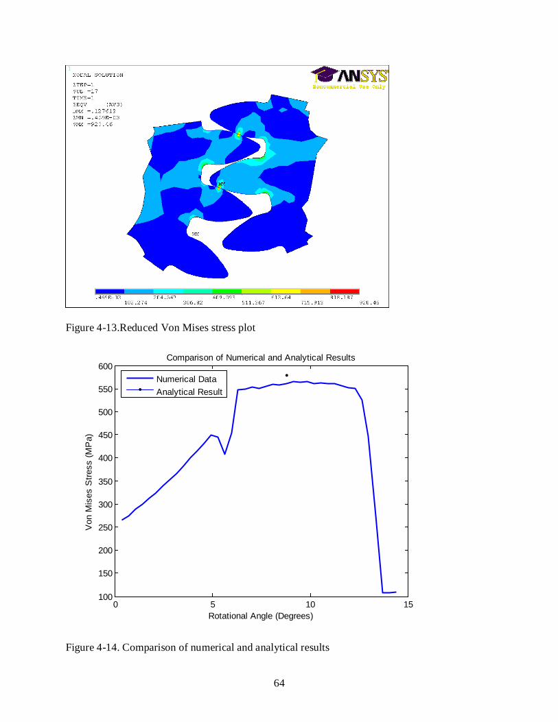
64
Figure 4-13.Reduced Von Mises stress plot
0 5 10 15100
150
200
250
300
350
400
450
500
550
600
Rotational Angle (Degrees)
Von
Mis
es S
tress
(MP
a)
Comparison of Numerical and Analytical Results
Numerical DataAnalytical Result
Figure 4-14. Comparison of numerical and analytical results
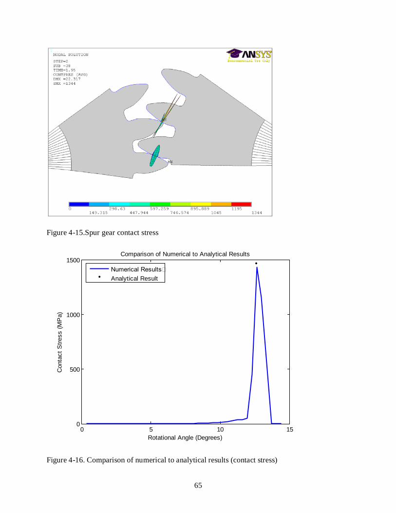
65
Figure 4-15.Spur gear contact stress
0 5 10 150
500
1000
1500
Rotational Angle (Degrees)
Con
tact
Stre
ss (M
Pa)
Comparison of Numerical to Analytical Results
Numerical ResultsAnalytical Result
Figure 4-16. Comparison of numerical to analytical results (contact stress)
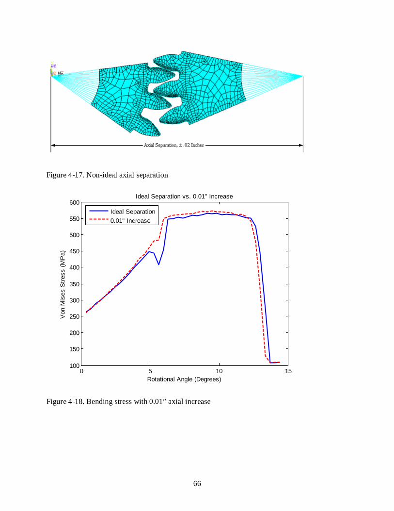
66
Figure 4-17. Non-ideal axial separation
0 5 10 15100
150
200
250
300
350
400
450
500
550
600
Rotational Angle (Degrees)
Von
Mis
es S
tress
(MP
a)
Ideal Separation vs. 0.01" Increase
Ideal Separation0.01" Increase
Figure 4-18. Bending stress with 0.01” axial increase
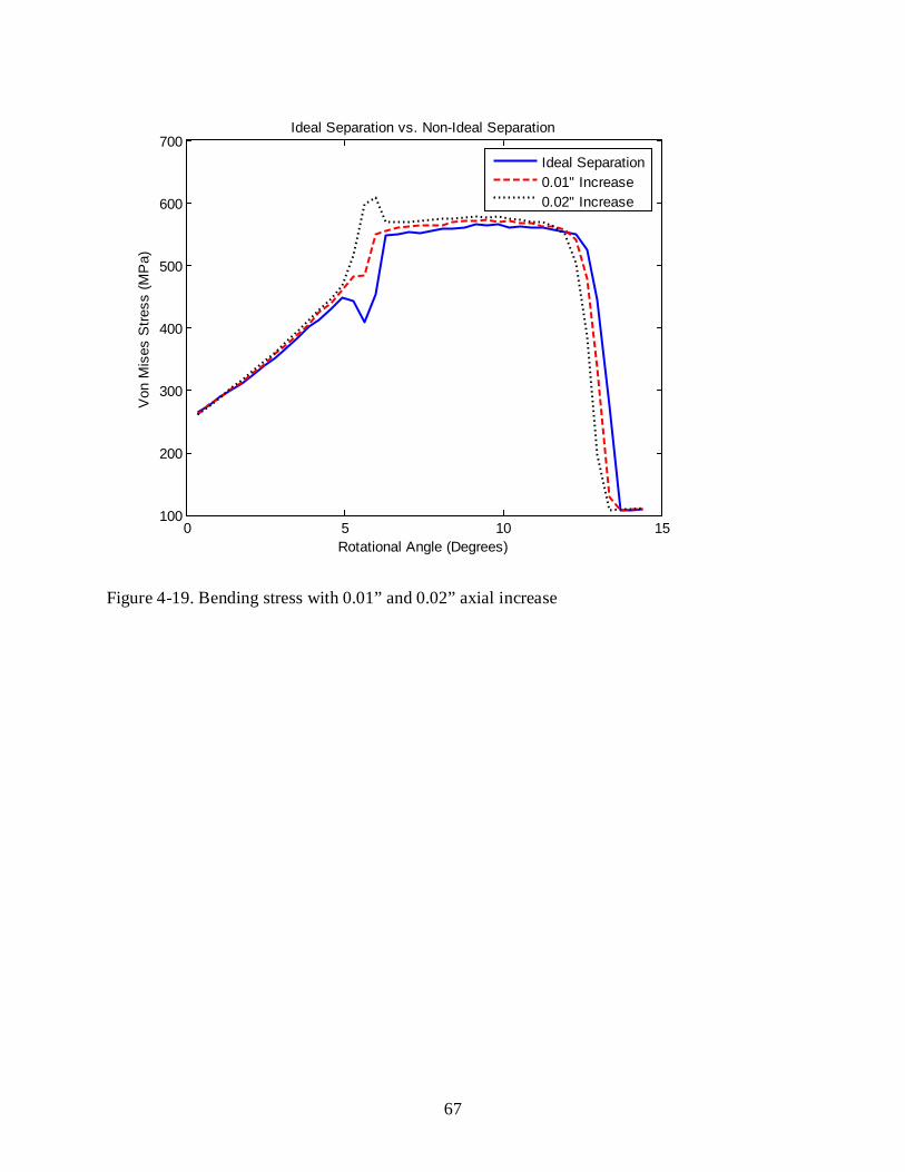
67
0 5 10 15100
200
300
400
500
600
700
Rotational Angle (Degrees)
Von
Mis
es S
tress
(MP
a)Ideal Separation vs. Non-Ideal Separation
Ideal Separation0.01" Increase0.02" Increase
Figure 4-19. Bending stress with 0.01” and 0.02” axial increase
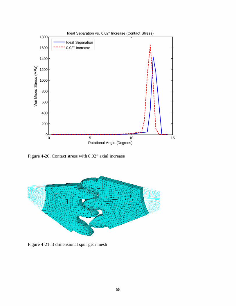
68
0 5 10 150
200
400
600
800
1000
1200
1400
1600
1800
Rotational Angle (Degrees)
Von
Mis
es S
tress
(MP
a)Ideal Separation vs. 0.02" Increase (Contact Stress)
Ideal Separation0.02" Increase
Figure 4-20. Contact stress with 0.02” axial increase
Figure 4-21. 3 dimensional spur gear mesh
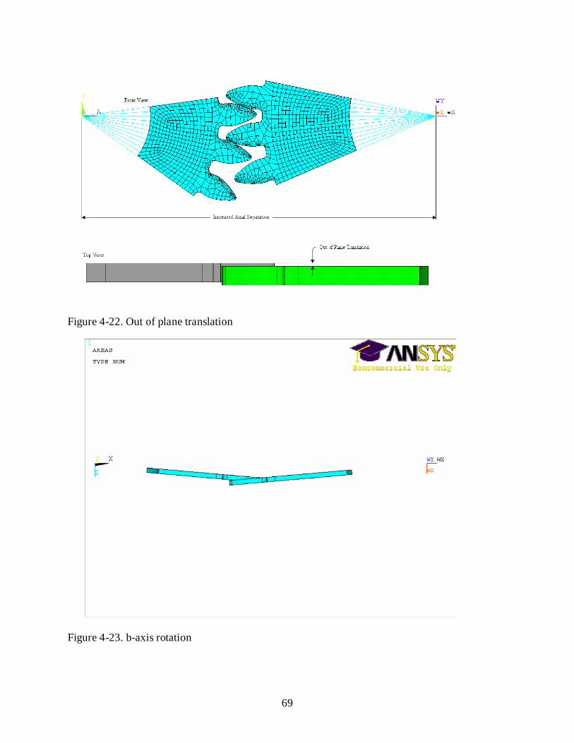
69
Figure 4-22. Out of plane translation
Figure 4-23. b-axis rotation
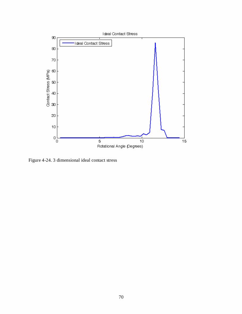
70
Figure 4-24. 3 dimensional ideal contact stress
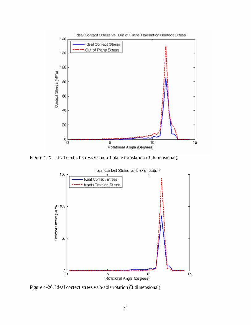
71
Figure 4-25. Ideal contact stress vs out of plane translation (3 dimensional)
Figure 4-26. Ideal contact stress vs b-axis rotation (3 dimensional)
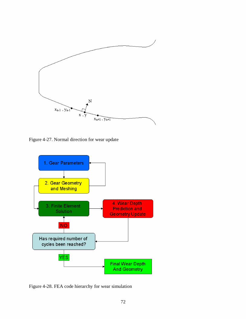
72
Figure 4-27. Normal direction for wear update
Figure 4-28. FEA code hierarchy for wear simulation
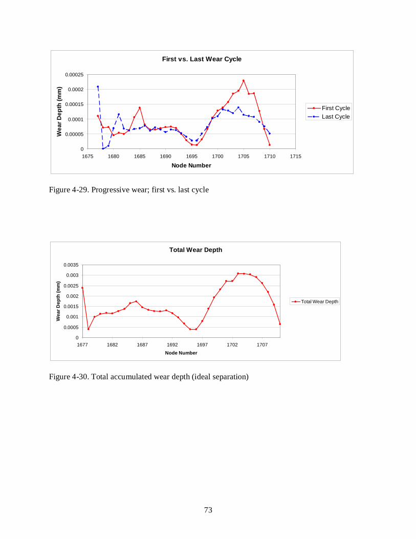
73
First vs. Last Wear Cycle
0
0.00005
0.0001
0.00015
0.0002
0.00025
1675 1680 1685 1690 1695 1700 1705 1710 1715
Node Number
Wea
r Dep
th (m
m)
First CycleLast Cycle
Figure 4-29. Progressive wear; first vs. last cycle
Total Wear Depth
0
0.0005
0.001
0.0015
0.002
0.0025
0.003
0.0035
1677 1682 1687 1692 1697 1702 1707
Node Number
Wea
r Dep
th (m
m)
Total Wear Depth
Figure 4-30. Total accumulated wear depth (ideal separation)
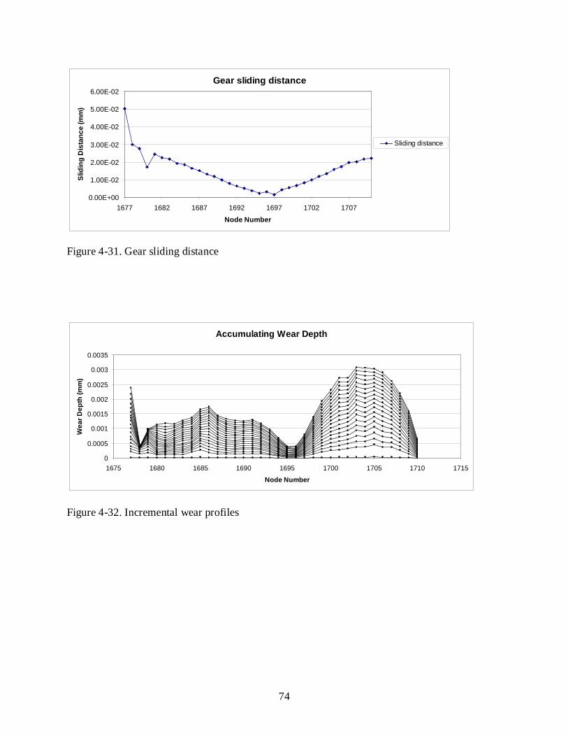
74
Gear sliding distance
0.00E+00
1.00E-02
2.00E-02
3.00E-02
4.00E-02
5.00E-02
6.00E-02
1677 1682 1687 1692 1697 1702 1707
Node Number
Slid
ing
Dis
tanc
e (m
m)
Sliding distance
Figure 4-31. Gear sliding distance
Accumulating Wear Depth
0
0.0005
0.001
0.0015
0.002
0.0025
0.003
0.0035
1675 1680 1685 1690 1695 1700 1705 1710 1715
Node Number
Wea
r Dep
th (m
m)
Figure 4-32. Incremental wear profiles
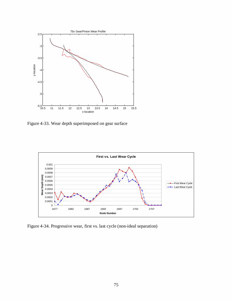
75
10.5 11 11.5 12 12.5 13 13.5 14 14.5 15 15.5-5.5
-5
-4.5
-4
-3.5
-3
-2.5
x-location
y-lo
catio
n75x Gear/Pinion Wear Profile
Figure 4-33. Wear depth superimposed on gear surface
First vs. Last Wear Cycle
00.00010.00020.00030.00040.00050.00060.00070.00080.0009
0.001
1677 1682 1687 1692 1697 1702 1707
Node Number
Wea
r Dep
th (m
m)
First Wear CycleLast Wear Cycle
Figure 4-34. Progressive wear, first vs. last cycle (non-ideal separation)
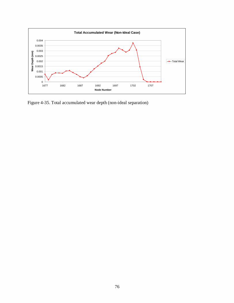
76
Total Accumulated Wear (Non-Ideal Case)
0
0.0005
0.001
0.0015
0.002
0.0025
0.003
0.0035
0.004
1677 1682 1687 1692 1697 1702 1707
Node Number
Wea
r Dep
th (m
m)
Total Wear
Figure 4-35. Total accumulated wear depth (non-ideal separation)
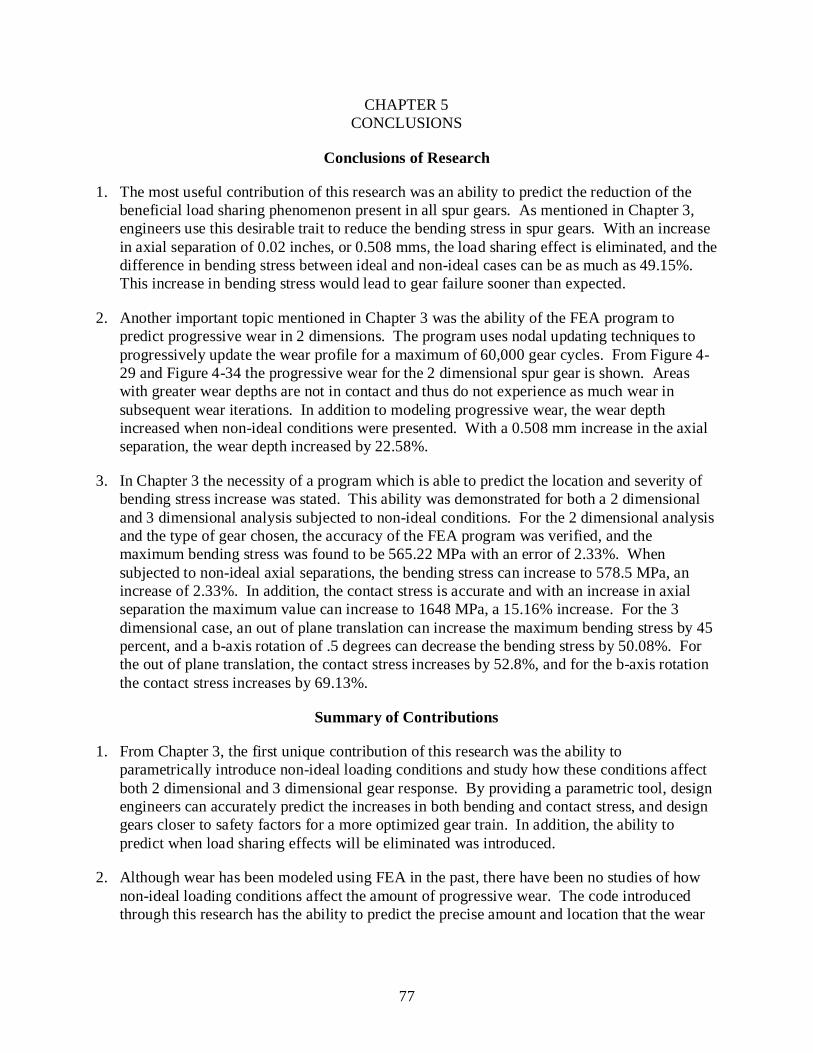
77
CHAPTER 5 CONCLUSIONS
Conclusions of Research
1. The most useful contribution of this research was an ability to predict the reduction of the beneficial load sharing phenomenon present in all spur gears. As mentioned in Chapter 3, engineers use this desirable trait to reduce the bending stress in spur gears. With an increase in axial separation of 0.02 inches, or 0.508 mms, the load sharing effect is eliminated, and the difference in bending stress between ideal and non-ideal cases can be as much as 49.15%. This increase in bending stress would lead to gear failure sooner than expected.
2. Another important topic mentioned in Chapter 3 was the ability of the FEA program to predict progressive wear in 2 dimensions. The program uses nodal updating techniques to progressively update the wear profile for a maximum of 60,000 gear cycles. From Figure 4-29 and Figure 4-34 the progressive wear for the 2 dimensional spur gear is shown. Areas with greater wear depths are not in contact and thus do not experience as much wear in subsequent wear iterations. In addition to modeling progressive wear, the wear depth increased when non-ideal conditions were presented. With a 0.508 mm increase in the axial separation, the wear depth increased by 22.58%.
3. In Chapter 3 the necessity of a program which is able to predict the location and severity of bending stress increase was stated. This ability was demonstrated for both a 2 dimensional and 3 dimensional analysis subjected to non-ideal conditions. For the 2 dimensional analysis and the type of gear chosen, the accuracy of the FEA program was verified, and the maximum bending stress was found to be 565.22 MPa with an error of 2.33%. When subjected to non-ideal axial separations, the bending stress can increase to 578.5 MPa, an increase of 2.33%. In addition, the contact stress is accurate and with an increase in axial separation the maximum value can increase to 1648 MPa, a 15.16% increase. For the 3 dimensional case, an out of plane translation can increase the maximum bending stress by 45 percent, and a b-axis rotation of .5 degrees can decrease the bending stress by 50.08%. For the out of plane translation, the contact stress increases by 52.8%, and for the b-axis rotation the contact stress increases by 69.13%.
Summary of Contributions
1. From Chapter 3, the first unique contribution of this research was the ability to parametrically introduce non-ideal loading conditions and study how these conditions affect both 2 dimensional and 3 dimensional gear response. By providing a parametric tool, design engineers can accurately predict the increases in both bending and contact stress, and design gears closer to safety factors for a more optimized gear train. In addition, the ability to predict when load sharing effects will be eliminated was introduced.
2. Although wear has been modeled using FEA in the past, there have been no studies of how non-ideal loading conditions affect the amount of progressive wear. The code introduced through this research has the ability to predict the precise amount and location that the wear
78
profile will change. This will prove useful when specifying the material type or hardness requirements when non-ideal loading may be expected to occur.
Future Research
1. The most important future research that should be considered would be to continue the 3 dimensional wear code. The main obstacle for this code is properly determining the normal directions of each node along the contact surface. With this normal direction computation an ability for node numbering independence is desired. Much painstaking effort could be implemented to manually compute normal directions by recording nodal connectivity and computing normal vectors via cross product operations. Another method which could compute these vectors without knowledge of the node numbers or neighboring nodes would be useful.
2. Once the 3 dimensional wear code has been developed, the next logical step would be to study the effects of non-ideal loading on the wear profile. The 3 dimensional spur gear FEA code can accommodate many different non-ideal loading conditions, and the insight of how this affects wear depth would be useful.
3. Another research topic would be to introduce different types of gears. Spur gears are the most simple type of gear, and many other designs are in use today. The ability to model and analyze these different gears would be greatly beneficial
4. An optimization problem of the gear shape to reduce bending stress, contact stress and wear depth would benefit the gear design community. Some research has been completed on this topic, and the next step would be to include non-ideal loading and wear depth calculations.
5. Finally, an experimental test rig to validate the theoretical assumptions of Archard’s wear law and the Finite Element Analysis would be a good research topic. Because a typical metallic gear may experience millions of cycles before appreciable wear is noticed, nylon gears would be the ideal choice for a wear analysis. Nylon gears should be mounted on shafts which are supported by bearings, with the drive shaft connected to an electrical motor. Because of the high wear rate of nylon along with a much easier material to deform, the input torque should be no more than 3.5 N-m. The application of this torque should be brought about by a clutch mechanism or similar device applied to the shaft not connected to the motor. Other experimental test rigs to date have used a combination of pre-loading a torsion bar with a defined strain which is measured by a strain gauge. The baseline wear should be calculated by a measured mass loss of the nylon gear, along with a tooth profile measurement. Non-ideal conditions can be imposed by precisely machining a mounting plate for the shaft not connected to the motor. Very precise mounting holes can be drilled corresponding to increases in axial separation, out of plane translation and b-axis rotation. The response of the nylon gear can then be determined after the appropriate number of cycles have been run.
79
LIST OF REFERENCES
[1] W Lewis, Investigation of the Strength of Gear Teeth. Proceedings of Engineering Club, Philadelphia, PA, 1893. p. 16-23
[2] Thomas J. Dolan, Edward L. Broghamer, A Photoelastic Study of Stresses in Gear Tooth Fillets. Engineering Experiment Station Bulletin Series No. 335, University of Illinois, Urbana-Champaign, 1942
[3] Paul H. Black, An Investigation of Relative Stresses in Solid Spur Gears by the Photoelastic Method. Engineering Experiment Station Bulletin Series No. 288, University of Illinois, Urbana-Champaign, 1936
[4] S. Shimamura, Noguchi Y., An Analytical Determination of Speed Factor in Gear Designs. Second SESA International Congress on Experimental Mechanics, Washington, D.C., 1965
[5] AGMA Standard for Rating the Pitting Resistance and Bending Strength of Spur and Helical Involute Gear Teeth. AGMA 218.01, American Gear Manufacturers Association , Dec. 1982.
[6] Sahir Arikan, Direct Calculation of AGMA Geometry Factor J by Making use of Polynomial Equations. Mechanics Research Communications, Volume 29, Issue 4 2002
[7] Tae Hyong Chong, Inho Bae, Gyung-Jin, Park, A new and generalized methodology to design multi-stage gear drives by integrating the dimensional and the configuration design process., Mechanism and Machine Theory, Volume 37, Issue 3
[8] Dennis P. Townsend, John J. Coy, Gearing. NASA Reference Publication. AVSCOM Technical Report 84-C-15 1985
[9] S. Vijayarangan, N. Ganesan, A Study of Dynamic Stresses in a Spur Gear Under a Moving Line Load and Impact Load Conditions by a Three-dimensional Finite Element Method. Journal of Sound and Vibration (1993) 162(1), 185-189
[10] Jiande Wang, Ian Howard, Finite Element Analysis of High Contact Ratio Spur Gears in Mesh. Rotating Machinery Research Group, Dept. of Mechanical Engineering, Curtin University of Technology, Australia. Journal of Tribology July 2005, Vol. 127
[11] Kadir Cavdar, Fatih Karpat, Fatih Babalik, Computer Aided Analysis of Bending Strength of Involute Spur Gears with Asymmetric Profile. Journal of Mechanical Design. May 2005, Vol. 127
[12] Alexander Kapelevich, Yuriy Shekhtman, Direct Gear Design: Bending Stress Minimization. Gear Technology, September/October 2003
[13] J.F. Archard, Contact and Rubbing of Flat Surfaces. J. Appl. Phys. 24 (1953) 981-988
[14] Anders Flodin, Soren Andersson, Simulation of Mild Wear in Spur Gears. Wear 207 (1997) 16-23
80
[15] A Sackfield, D A Hills, Some Useful Results in the Classical Hertz Contact Problem, The Journal of Strain Analysis for Engineering Design Volume 18, Number 2 / 1983
[16] Robert C. Juvinall, Kurt M. Marshek, Fundamentals of Machine Component Design, John Wiley and Sons, Inc 1983
[17] Alexander Kapelevich, Geometry and Design of Involute Spur Gears with Asymmetric Teeth, Mechanism and Machine Theory, Volume 35, Issue 1, January 2000, Pages 117-130
[18] M H Arafa, M M Megahed, Evaluation of Spur Gear Mesh Compliance Using the Finite Element Method, Proc Instn Mech Engrs Vol 213 Part C, 1999
[19] J.F. Archard, W. Hirst, The Wear of Metals under Unlubricated Conditions, Proceedings of the Royal Society of London. Series A, Mathematical and Physical Sciences, Volume 236, Number 1206 / August 02, 1956
[20] P.M. Ku, Gear Failure Modes – Importance of Lubrication and Mechanics, Tribology Transactions, Volume 19, Issue 3 July 1976, pages 239-249
[21] Anders Flodin, Wear Investigation of Spur Gear Teeth, Tribotest Journal 7-1, September 2000
[22] H Winter, K Michaelis, FZG Gear Test Rig – Description and Possibilities, Coordinate European Council Second International Symposium 1985
[23] Anders Flodin, Soren Andersson, Simulation of Mild Wear in Spur Gears, Wear 207 (1997) 16-23
[24] Olle Lundvall, Anders Klarbring, Simulation of Wear by Use of A Nonsmooth Newton Method – A Spur Gear Application, Mech. Struc. and Mach., 29(2), 223-228 (2001)
[25] Josef Wojnarowski, Valentin Onishchenko, Tooth Wear Effects on Spur Gear Dynamics, Mechanism and Machine Theory 38 (2003) 161-178
[26] Anders Flodin, Wear of Spur and Helical Gears, Doctoral Thesis, Department of Machine Design, Royal Institute of Technology, S-100 Stockholm, Sweden (2000)
[27] S Senthilvelan, R Gnanamoorthy, Wear Characteristics of injection-moulded unfilled and glass-filled nylon 6 spur gears, Proc. Instn. Mech. Engrs., Vol 218 Part J (2004)
[28] M. Kalin, J. Vizintin, The tribological performance of DLC-coated gears lubricated with biodegradable oil in various pinon/gear material combinations, Wear 259 (2005) 1270-1280
[29] P. Velex, M. Maatar, A Mathematical Model for Analyzing the Influence of Shape Deviations and Mounting Errors on Gear Dynamic Behaviour, Journal of Sound and Vibration (1996) 191(5), 629-660
81
[30] A Parey, N Tandon, Spur Gear Dynamic Models Including Defects, A Review, The Shock and Vibration Digest, 2003
[31] Sandro Barone, Leonardo Borgianni, Paola Forte, Evaluation of the Effect of Misalignment and Profile Modification in Face Gear Drive by a Finite Element Meshing Simulation, ASME Vol. 126, September 2004
[32] Shuting Li, Finite element analyses for contact strength and bending strength of a pair of spur gears with machining errors, assembly errors and tooth modifications, Mechanism and Machine Theory, Volume 42, Issue 1, January 2007, Pages 88-114
[33] Didier Remond, Practical Performances of high-speed measurement of gear transmission error or torsional vibrations with optical encoders, Meas. Sci. Technol. 9 (1998) 347-353
[34] M. Guagliano, E. Riva, M. Guidetti, Contact Fatigue Failure Analysis of Shot-Peened Gears, Engineering Failure Analysis, Volume 9, Issue 2, April 2002, Pages 147-158
[35] P.J.L. Fernandes, Tooth Bending Fatigue Failures in Gears, Engineering Failure Analysis, Vol. 3, pp. 219-225 1996
[36] C.R. Das, S.K. Albert, A.K. Bhaduri, S.K. Ray, Failure Analysis of a Pinion, Engineering Failure Analysis, Volume 12, Issue 2, April 2005, Pages 287-298
[37] Dennis P. Townsend, Gear and Transmission Research at NASA Lewis Research Center, NASA Technical Memorandum 107428 1997
[38] J.R. Colbourne, The Geometry of Involute Gears, Springer-Verlag 1987
[39] R.E. Peterson, Stress Concentration Design Factors, Wiley, New York 1953
[40] Dolan, T.J. and Broghame, E.L., A Photoelastic Study of Stresses in Gear tooth Fillets, Univ. Illinois Eng. Expt. Sta. Bull. 335, March 1942
[41] Michael Griffis, Proving Dooner’s Third Law of Gearing: A Study of Curvature, The Eigenpoint Company, Gainesville, FL USA
[42] Joseph E. Shigley, Charles R. Mischke, Richard G. Budynas, Mechanical Engineering Design Seventh Edition, McGraw-Hill, 2004
[43] Weisstein, Eric W., “Involute.” From MathWorld – A Wolfram Web Resource http://mathworld.wolfram.com/Involute.html
[44] ANSYS, Release 11.0 Documentation for ANSYS, 3.6 General Element Formulations
[45] C. James Li, Hyungdae Lee, Gear fatigue crack prognosis using embedded model, gear dynamic model and fracture mechanics, Mechanical Systems and Signal Processing, Volume 19, Issue 4, July 2005, Pages 836-846
82
[46] ANSYS, Release 11.0 Documentation for ANSYS, MPC 184-Link/Beam Multipoint Constraint Element: Rigid Link or Rigid Beam
[47] Kenneth Nowaczyk, courtesy of: GearLab, The Ohio State University, March 19, 2008
[48] J J Kauzlarich, J A Williams, Archard Wear and Component Geometry, Proc Instn Mech Engs Vol 215 Part J
[49] Pritt Podra, Soren Andersson, Simulating sliding wear with finite element method, Tribology International, Volume 32, Issue 2, February 1999, Pages 71-81
[50] D. Walton, A.J. Goodwin, The wear of unlubricated metallic spur gears, Wear 222 (1998) 103-113
[51] Anders Flodin, Wear of Spur and Helical Gears, Doctoral Thesis, Department of Machine Design, Royal Institute of Technology, S-100 44 Stockholm, Sweden
83
BIOGRAPHICAL SKETCH
Kyle Stoker began his undergraduate course work at the University of Florida in August
2002. He graduated cum laude in May 2007 with a Bachelor of Science in mechanical
engineering. Kyle then continued his education at the University of Florida under the advisory
of Dr. Nam Ho Kim. Kyle will be receiving a Master of Science in mechanical engineering in
May of 2009.


![[1] involuteΣiii(spur and helical gear design system)Spur...1 [1] involuteΣiii(spur and helical gear design system) 図1.1 involuteΣiii(spur and helical) 1.1 概要 involuteΣⅲ(spur](https://img.pdfslide.net/doc/110x75/5ae0683d7f8b9a97518d2bd7/1-involuteiiispur-and-helical-gear-design-system-spur1-1-involuteiiispur.jpg)