A FIRST COURSE INDYNAMICS

with a Panorama of RecentDevelopments

BORIS HASSELBLATTTufts University

ANATOLE KATOKThe Pennsylvania State University

PUBLISHED BY THE PRESS SYNDICATE OF THE UNIVERSITY OF CAMBRIDGE

The Pitt Building, Trumpington Street, Cambridge, United Kingdom

CAMBRIDGE UNIVERSITY PRESS

The Edinburgh Building, Cambridge CB2 2RU, UK40 West 20th Street, New York, NY 10011-4211, USA477 Williamstown Road, Port Melbourne, VIC 3207, AustraliaRuiz de Alarcon 13, 28014 Madrid, SpainDock House, The Waterfront, Cape Town 8001, South Africa

http://www.cambridge.org

C© Boris Hasselblatt and Anatole Katok 2003

This book is in copyright. Subject to statutory exceptionand to the provisions of relevant collective licensing agreements,no reproduction of any part may take place withoutthe written permission of Cambridge University Press.

First published 2003

Printed in the United States of America

Typefaces Utopia 9.75/13 pt., Optima and Bodoni System LATEX 2ε [tb]

A catalog record for this book is available from the British Library.

Library of Congress Cataloging in Publication Data

Hasselblatt, Boris.A first course in dynamics : with a panorama of recent developments /

Boris Hasselblatt, Anatole Katok.p. cm.

Includes bibliographical references and index.ISBN 0-521-58304-7 – ISBN 0-521-58750-6 (pb.)

1. Differentiable dynamical systems. I. Katok, A. B. II. Title.QA614.8 .H38 2002514′.74–dc21 2002019246

ISBN 0 521 58304 7 hardbackISBN 0 521 58750 6 paperback

Contents

Preface page ix

1 Introduction 11.1 Dynamics 11.2 Dynamics in Nature 41.3 Dynamics in Mathematics 19

PART 1. A COURSE IN DYNAMICS: FROM SIMPLE TO

COMPLICATED BEHAVIOR 29

2 Systems with Stable Asymptotic Behavior 312.1 Linear Maps and Linearization 312.2 Contractions in Euclidean Space 322.3 Nondecreasing Maps of an Interval and Bifurcations 452.4 Differential Equations 492.5 Quadratic Maps 572.6 Metric Spaces 612.7 Fractals 69

3 Linear Maps and Linear Differential Equations 733.1 Linear Maps in the Plane 733.2 Linear Differential Equations in the Plane 863.3 Linear Maps and Differential Equations in Higher Dimension 90

4 Recurrence and Equidistribution on the Circle 964.1 Rotations of the Circle 964.2 Some Applications of Density and Uniform Distribution 1094.3 Invertible Circle Maps 1234.4 Cantor Phenomena 135

5 Recurrence and Equidistribution in Higher Dimension 1435.1 Translations and Linear Flows on the Torus 1435.2 Applications of Translations and Linear Flows 152

v

vi Contents

6 Conservative Systems 1556.1 Preservation of Phase Volume and Recurrence 1556.2 Newtonian Systems of Classical Mechanics 1626.3 Billiards: Definition and Examples 1776.4 Convex Billiards 186

7 Simple Systems with Complicated Orbit Structure 1967.1 Growth of Periodic Points 1967.2 Topological Transitivity and Chaos 2057.3 Coding 2117.4 More Examples of Coding 2217.5 Uniform Distribution 2297.6 Independence, Entropy, Mixing 235

8 Entropy and Chaos 2428.1 Dimension of a Compact Space 2428.2 Topological Entropy 2458.3 Applications and Extensions 251

PART 2. PANORAMA OF DYNAMICAL SYSTEMS 257

9 Simple Dynamics as a Tool 2599.1 Introduction 2599.2 Implicit- and Inverse-Function Theorems in Euclidean Space 2609.3 Persistence of Transverse Fixed Points 2659.4 Solutions of Differential Equations 2679.5 Hyperbolicity 273

10 Hyperbolic Dynamics 27910.1 Hyperbolic Sets 27910.2 Orbit Structure and Orbit Growth 28410.3 Coding and Mixing 29110.4 Statistical Properties 29410.5 Nonuniformly Hyperbolic Dynamical Systems 298

11 Quadratic Maps 29911.1 Preliminaries 29911.2 Development of Simple Behavior Beyond the First Bifurcation 30311.3 Onset of Complexity 30711.4 Hyperbolic and Stochastic Behavior 314

12 Homoclinic Tangles 31812.1 Nonlinear Horseshoes 31812.2 Homoclinic Points 32012.3 The Appearance of Horseshoes 32212.4 The Importance of Horseshoes 32412.5 Detecting Homoclinic Tangles: The Poincare–Melnikov

Method 32712.6 Homoclinic Tangencies 328

Contents vii

13 Strange Attractors 33113.1 Familiar Attractors 33113.2 The Solenoid 33313.3 The Lorenz Attractor 335

14 Variational Methods, Twist Maps, and Closed Geodesics 34214.1 The Variational Method and Birkhoff Periodic Orbits

for Billiards 34214.2 Birkhoff Periodic Orbits and Aubry–Mather Theory

for Twist Maps 34614.3 Invariant Circles and Regions of Instability 35714.4 Periodic Points for Maps of the Cylinder 36014.5 Geodesics on the Sphere 362

15 Dynamics, Number Theory, and Diophantine Approximation 36515.1 Uniform Distribution of the Fractional Parts of Polynomials 36515.2 Continued Fractions and Rational Approximation 36915.3 The Gauß Map 37415.4 Homogeneous Dynamics, Geometry, and Number Theory 37715.5 Quadratic Forms in Three Variables 383

Reading 386

APPENDIX 389A.1 Metric Spaces 389A.2 Differentiability 400A.3 Riemann Integration in Metric Spaces 401

Hints and Answers 408

Solutions 414

Index 419

CHAPTER 1

Introduction

This chapter is a prelude to this book. It first describes in general terms what thediscipline of dynamical systems is about. The following sections contain a largenumber of examples. Some of the problems treated later in the book appear herefor the first time.

1.1 DYNAMICS

What is a dynamical system? It is dynamical, something happens, somethingchanges over time. How do things change in nature? Galileo Galilei and Isaac Newtonwere key players in a revolution whose central tenet is Nature obeys unchanginglaws that mathematics can describe. Things behave and evolve in a way determinedby fixed rules. The prehistory of dynamics as we know it is the development ofthe laws of mechanics, the pursuit of exact science, and the full development ofclassical and celestial mechanics. The Newtonian revolution lies in the fact thatthe principles of nature can be expressed in terms of mathematics, and physicalevents can be predicted and designed with mathematical certainty. After mechanics,electricity, magnetism, and thermodynamics, other natural sciences followed suit,and in the social sciences quantitative deterministic descriptions also have taken ahold.

1.1.1 Determinism Versus PredictabilityThe key word is determinism: Nature obeys unchanging laws. The regularity ofcelestial motions has been the primary example of order in nature forever:

God said, let there be lights in the firmament of the heavens to divide the day from thenight and let them be for signs and for seasons and for days and years.

The successes of classical and especially celestial mechanics in the eighteenth andnineteenth centuries were seemingly unlimited, and Pierre Simon de Laplace feltjustified in saying (in the opening passage he added to his 1812 Philosophical Essay

1

2 1. Introduction

on Probabilities):

We ought then to consider the present state of the universe as the effects of its pre-vious state and as the cause of that which is to follow. An intelligence that, at a giveninstant, could comprehend all the forces by which nature is animated and the respec-tive situation of the beings that make it up, if moreover it were vast enough to submitthese data to analysis, would encompass in the same formula the movements of thegreatest bodies of the universe and those of the lightest atoms. For such an intelli-gence nothing would be uncertain, and the future, like the past, would be open to itseyes.1

The enthusiasm in this 1812 overture is understandable, and this forceful descrip-tion of determinism is a good anchor for an understanding of one of the ba-sic aspects of dynamical systems. Moreover, the titanic life’s work of Laplace incelestial mechanics earned him the right to make such bold pronouncements.There are some problems with this statement, however, and a central missionof dynamical systems and of this book is to explore the relation between de-terminism and predictability, which Laplace’s statement misses. The history ofthe modern theory of dynamical systems begins with Henri Jules Poincare inthe late nineteenth century. Almost 100 years after Laplace he wrote a summaryrejoinder:

If we could know exactly the laws of nature and the situation of the universe at theinitial instant, we should be able to predict exactly the situation of this same universeat a subsequent instant. But even when the natural laws should have no further secretfor us, we could know the initial situation only approximately. If that permits us toforesee the subsequent situation with the same degree of approximation, this is all werequire, we say the phenomenon has been predicted, that it is ruled by laws. But thisis not always the case; it may happen that slight differences in the initial conditionsproduce very great differences in the final phenomena; a slight error in the formerwould make an enormous error in the latter. Prediction becomes impossible and wehave the fortuitous phenomenon.2

His insights led to the point of view that underlies the study of dynamics as it ispracticed now and as we present it in this book: The study of long-term asymptoticbehavior, and especially that of its qualitative aspects, requires direct methods thatdo not rely on prior explicit calculation of solutions. And in addition to the qual-itative (geometric) study of a dynamical system, probabilistic phenomena play arole.

A major motivation for the study of dynamical systems is their pervasive im-portance in dealing with the world around us. Many systems evolve continuouslyin time, such as those in mechanics, but there are also systems that naturallyevolve in discrete steps. We presently describe models of, for example, butterflypopulations, that are clocked by natural cycles. Butterflies live in the summer, and

1 Pierre Simon marquis de Laplace, Philosophical Essay on Probabilities, translated from the fifthFrench edition of 1925 by Andrew I. Dale, Springer-Verlag, New York, 1995, p. 2.

2 Henri Jules Poincare, Science et methode, Section IV.II., Flammarion 1908; see The Foundations ofScience; Science and Hypothesis, The Value of science, Science and Method, translated by George BruceHalsted, The Science Press, Lancaster, PA, 1946, pp. 397f; The Value of Science: Essential Writings ofHenri Poincare, edited by Stephen Jay Gould, Modern Library, 2001.

1.1 Dynamics 3

we discuss laws describing how next summer’s population size is determined bythat of this summer. There are also ways of studying a continuous-time systemby making it look like a discrete-time system. For example, one might check onthe moon’s position precisely every 24 hours. Or one could keep track of whereit rises any given day. Therefore we allow dynamical systems to evolve in dis-crete steps, where the same rule is applied repeatedly to the result of the previousstep.

This is important for another reason. Such stepwise processes do not only oc-cur in the world around us, but also in our minds. This happens whenever we gothrough repeated steps on our way to the elusive perfect solution. Applied to suchprocedures, dynamics provides insights and methods that are useful in analysis. Weshow in this book that important facts in analysis are consequences of dynamicalfacts, even of some rather simple ones: The Contraction Principle (Proposition 2.2.8,Proposition 2.2.10, Proposition 2.6.10) gives the Inverse-Function Theorem 9.2.2and the Implicit-Function Theorem 9.2.3. The power of dynamics in situations ofthis kind has to do with the fact that various problems can be approached with aniterative procedure of successive approximation by improved guesses at an answer.Dynamics naturally provides the means to understand where such a procedureleads.

1.1.2 Dynamics in AnalysisWhenever you use a systematic procedure to improve a guess at a solution you arelikely to have found a way of using dynamics to solve your problem exactly. To beginto appreciate the power of this approach it is important to understand that the iter-ative processes dynamics can handle are not at all required to operate on numbersonly. They may manipulate quite complex classes of objects: numbers, points inEuclidean space, curves, functions, sequences, mappings, and so on. The possibil-ities are endless, and dynamics can handle them all. We use iteration schemes onfunctions in Section 9.4, mappings in Section 9.2.1 and sequences in Section 9.5.The beauty of these applications lies in the elegance, power, and simplicity of thesolutions and insights they provide.

1.1.3 Dynamics in MathematicsThe preceding list touches only on a portion of the utility of dynamical systemsin understanding mathematical structures. There are others, where insights intocertain patterns in some branches of mathematics are most easily obtained byperceiving that underlying the structure in question is something of a dynamicalnature that can readily be analyzed or, sometimes, has been analyzed already. Thisis a range of applications of dynamical ideas that is exciting because it often involvesphenomena of a rich subtlety and variety. Here the beauty of applying dynamicalsystems lies in the variety of behaviors, the surprising discovery of order in bewil-dering complexity, and in the coherence between different areas of mathematicsthat one may discover. A little later in this introductory chapter we give some simpleexamples of such situations.

4 1. Introduction

� EXERCISESIn these exercises you are asked to use a calculator to play with some simple iterativeprocedures. These are not random samples, and we return to several of these indue course. In each exercise you are given a function f as well as a number x0. Theassignment is to consider the sequence defined recursively by the given initial valueand the rule xn+1 = f (xn). Compute enough terms to describe what happens in thelong run. If the sequence converges, note the limit and endeavor to determine aclosed expression for it. Note the number of steps you needed to compute to seethe pattern or to get a good approximation of the limit.

� Exercise 1.1.1 f (x) = √2+ x, x0 = 1.

� Exercise 1.1.2 f (x) = sin x, x0 = 1. Use the degree setting on your calculator –this means that (in radians) we actually compute f (x) = sin(πx/180).

� Exercise 1.1.3 f (x) = sin x, x0 = 1. Use the radian setting here and forever after.

� Exercise 1.1.4 f (x) = cos x, x0 = 1.

� Exercise 1.1.5

f (x) = x sin x + cos x1+ sin x

, x0 = 3/4.

� Exercise 1.1.6 f (x) = {10x} = 10x − �10x (fractional part), x0 =√

1/2.

� Exercise 1.1.7 f (x) = {2x}, x0 =√

1/2.

� Exercise 1.1.8

f (x) = 5+ x2

2x, x0 = 2.

� Exercise 1.1.9 f (x) = x − tan x, x0 = 1.

� Exercise 1.1.10 f (x) = kx(1− x), x0 = 1/2, k = 1/2, 1, 2, 3.1, 3.5, 3.83, 3.99, 4.

� Exercise 1.1.11 f (x) = x + e−x, x0 = 1.

1.2 DYNAMICS IN NATURE

1.2.1 Antipodal RabbitsRabbits are not indigenous to Australia, but 24 wild European rabbits were intro-duced by one Thomas Austin near Geelong in Southern Victoria around 1860, withunfortunate consequences. Within a decade they were rampant across Victoria,and within 20 years millions had devastated the land, and a prize of £25,000 wasadvertized for a solution. By 1910 their descendants had spread across most of thecontinent. The ecological impact is deep and widespread and has been called anational tragedy. The annual cost to agriculture is estimated at AU$600 million.The unchecked growth of their population makes an interesting example of adynamical system.

In modeling the development of this population we make a few choices. Itslarge size suggests to count it in millions, and when the number of rabbits is

1.2 Dynamics in Nature 5

expressed as x million then x is not necessarily an integer. After all, the initial valueis 0.000024 million rabbits. Therefore we measure the population by a real numberx. As for time, in a mild climate rabbits – famously – reproduce continuously.(This is different for butterflies, say, whose existence and reproduction are strictlyseasonal; see Section 1.2.9.) Therefore we are best served by taking the time variableto be a real number as well, t, say. Thus we are looking for ways of describing thenumber of rabbits as a function x(t) of time.

To understand the dependence on time we look at what rabbits do: They eatand reproduce. Australia is large, so they can eat all they want, and during any giventime period �t a fixed percentage of the (female) population will give birth and a(smaller) percentage will die of old age (there are no natural enemies). Thereforethe increment x(t +�t)− x(t) is proportional to x(t)�t (via the difference of birthand death rates). Taking a limit as �t → 0 we find that

dxdt= kx,(1.2.1)

where k represents the (fixed) relative growth rate of the population. Alternatively,we sometimes write x = kx, where the dot denotes differentiation with respect tot. By now you should recognize this model from your calculus class.

It is the unchanging environment (and biology) that gives rise to this unchang-ing evolution law and makes this a dynamical system of the kind we study. Thedifferential equation (1.2.1), which relates x and its rate of change, is easy to solve:Separate variables (all x on the left, all t on the right) to get (1/x)dx = k dt andintegrate this with respect to t using substitution:

log |x| =∫

1x

dx =∫

k dt = kt + C,

where log is the natural logarithm. Therefore, |x(t)| = eC ekt with eC = |x(0)| and wefind that

x(t) = x(0)ekt.(1.2.2)

� Exercise 1.2.1 Justify the disappearance of the absolute value signs above.

� Exercise 1.2.2 If x(0) = 3 and x(4) = 6, find x(2), x(6), and x(8).

1.2.2 The Leaning Rabbits of PisaIn the year 1202, Leonardo of Pisa considered a more moderate question regardingrabbits, which we explore in Example 2.2.9 and Section 3.1.9. The main differencesto the large-scale Australian model above are that the size of his urban yard limitedhim to small numbers of rabbits and that with such a small number the populationgrowth does not happen continuously, but in relatively substantial discrete steps.Here is the problem as he posed it:3

How many pairs of rabbits can be bred from one pair in one year?

3 Leonardo of Pisa: Liber abaci (1202), published in Scritti di Leonardo Pisano, Rome, B. Boncompagni,1857; see p. 3 of Dirk J. Struik, A Source Book in Mathematics 1200–1800, Princeton, NJ, PrincetonUniversity Press, 1986.

6 1. Introduction

A man has one pair of rabbits at a certain place entirely surrounded by a wall. Wewish to know how many pairs can be bred from it in one year, if the nature of theserabbits is such that they breed every month one other pair and begin to breed in thesecond month after their birth. Let the first pair breed a pair in the first month, thenduplicate it and there will be 2 pairs in a month. From these pairs one, namely the first,breeds a pair in the second month, and thus there are 3 pairs in the second month.From these in one month two will become pregnant, so that in the third month 2 pairsof rabbits will be born. Thus there are 5 pairs in this month. From these in the samemonth 3 will be pregnant, so that in the fourth month there will be 8 pairs . . . [Wehave done this] by combining the first number with the second, hence 1 and 2, and thesecond with the third, and the third with the fourth . . .

In other words, he came up with a sequence of numbers (of pairs of rabbits)governed by the recursion bn+1 = bn+ bn−1 and chose starting values b0 = b1 = 1,so the sequence goes 1, 1, 2, 3, 5, 8, 13, . . . . Does this look familiar? (Hint: As the sonof Bonaccio, Leonardo of Pisa was known as filius Bonacci or “son of good nature”;Fibonacci for short.) Here is a question that can be answered easily with a little bit ofdynamics: How does his model compare with the continuous exponential-growthmodel above?

According to exponential growth one should expect that once the terms getlarge we always have bn+1 ≈ abn for some constant a independent of n. If we pretendthat we have actual equality, then the recursion formula gives

a2bn = abn+1 = bn+2 = bn+1 + bn = (a+ 1)bn,

so we must have a2 = a+ 1. The quadratic formula then gives us the value of thegrowth constant a.

� Exercise 1.2.3 Calculate a.

Note, however, that we have only shown that if the growth is eventuallyexponential, then the growth constant is this a, not that the growth is eventuallyexponential. (If we assume the recursion bn+1 = 1 leads to exponential growth, wecould come up with a growth parameter if we are quick enough to do it before get-ting a contradiction.) Dynamics provides us with tools that enable us to verify thisproperty easily in various different ways (Example 2.2.9 and Section 3.1.9). In Propo-sition 3.1.11 we even convert this recursively defined sequence into closed form.

The value of this asymptotic ratio was known to Johannes Kepler. It is thegolden mean or the divine proportion. In his 1619 book Harmonices Mundi hewrote (on page 273):

there is the ratio which is never fully expressed in numbers and cannot be demon-strated by numbers in any other way, except by a long series of numbers graduallyapproaching it: this ratio is called divine, when it is perfect, and it rules in various waysthroughout the dodecahedral wedding. Accordingly, the following consonances beginto shadow forth that ratio: 1:2 and 2:3 and 3:5 and 5:8. For it exists most imperfectlyin 1:2, more perfectly in 5:8, and still more perfectly if we add 5 and 8 to make 13 andtake 8 as the numerator . . . .4

4 Johannes Kepler, Epitome of Copernican Astronomy & Harmonies of the World, Amherst, NY,Prometheus Books, 1995.

1.2 Dynamics in Nature 7

We note in Example 15.2.5 that these Fibonacci ratios are the optimal rationalapproximations of the golden mean.

� Exercise 1.2.4 Express 1+ 1+ 2+ 3+ · · · + bn in terms of bn+2.

1.2.3 Fine DiningOnce upon a time lobsters were so abundant in New England waters that theywere poor man’s food. It even happened that prisoners in Maine rioted to demandto be fed something other than lobsters for a change. Nowadays the haul is lessabundant and lobsters have become associated with fine dining. One (optimistic?)model for the declining yields stipulates that the catch in any given year shouldturn out to be the average of the previous two years’ catches.

Using again an for the number of lobsters caught in the year n, we can expressthis model by a simple recursion relation:

an+1 = an−1/2+ an/2.(1.2.3)

As initial values one can take the Maine harvests of 1996 and 1997, which were16,435 and 20,871 (metric) tons, respectively. This recursion is similar to the one forthe Fibonacci numbers, but in this case no exponential growth is to be expected.One can see from the recursion that all future yields should be between the twoinitial data. Indeed, 1997 was a record year. In Proposition 3.1.13 we find a way ofgiving explicit formulas for future yields, that is, we give the yield in an arbitraryyear n in a closed form as a function of n.

This situation as well as the Fibonacci rabbit problem are examples where timeis measured in discrete steps. There are many other examples where this is natural.Such a scenario from population biology is discussed in Section 1.2.9. Other biolog-ical examples arise in genetics (gene frequency) or epidemiology. Social scientistsuse discrete-time models as well (commodity prices, rate of spread of a rumor,theories of learning that model the amount of information retained for a giventime).

1.2.4 Turning Over a New LeafThe word phyllotaxis comes from the words phyllo=leaf and taxis=order or arrange-ment. It refers to the way leaves are arranged on twigs, or other plant componentson the next larger one. The seeds of a sunflower and of a pine cone are furtherexamples. A beautiful description is given by Harold Scott Macdonald Coxeter inhis Introduction to Geometry. That regular patterns often occur is familiar fromsunflowers and pineapples.

In some species of trees the leaves on twigs are also arranged in regular patterns.The pattern varies by species. The simplest pattern is that of leaves alternatingon opposite sides of the twig. It is called (1, 2)-phyllotaxis: Successive leaves areseparated by a half-turn around the twig. The leaves of elms exhibit this pattern, asdo hazel leaves.5 Adjacent leaves may also have a (2/3) turn between them, whichwould be referred to as (2, 3)-phyllotaxis. Such is the case with beeches. Oak trees

5 On which the first author of this book should be an expert!

8 1. Introduction

show a (3, 5)-pattern, poplars a (5, 8), and willows, (8, 13)-phyllotaxis. Of course,the pattern may not always be attained to full precision, and in some plants thereare transitions between different patterns as they grow.

The diamond-shaped seeds of a sunflower are packed densely and regularly.One may perceive a spiral pattern in their arrangement, and, in fact, there arealways two such patterns in opposite directions. The numbers of spirals in the twopatterns are successive Fibonacci numbers. The seeds of a fir cone exhibit spiralsas well, but on a cone rather than flat ones. These come in two families, whosenumbers are again successive Fibonacci numbers.

Pineapples, too, exhibit spiral patterns, and, because their surface is composedof approximately hexagonal pieces, there are three possible directions in whichone can perceive spirals. Accordingly, one may find 5, 8, and 13 spirals: 5 slopingup gently to the right, say, 8 sloping up to the left, and 13 sloping quite steeplyright.

The observation and enjoyment of these beautiful patterns is not new. Theywere noticed systematically in the nineteenth century. But an explanation for whythere are such patterns did not emerge particularly soon. In fact, the case is notentirely closed yet.

Here is a model that leads to an explanation of how phyllotaxis occurs. The basicgrowth process of this type consists of buds (primordia) of leaves or seeds growingout of a center and then moving away from it according to three rules proposed in1868 by the self-taught botanist Wilhelm Friedrich Benedikt Hofmeister, while hewas professor and director of the botanical garden in Heidelberg:

(1) New buds form at regular intervals, far from the old ones.(2) Buds move radially from the center.(3) The growth rate decreases as one moves outward.

A physical experiment designed to mimic these three Hofmeister rules producesspiral patterns of this Fibonacci type, so from these rules one should be able toinfer that spiral patterns must occur. This has been done recently with methods ofthe kind that this book describes.6

Here is a description of how dynamics may help. To implement the Hofmeisterrules we model the situation by a family of N + 1 concentric circles of radiusrk (k = 0, . . . , N ), where r stands for growth rate, and we put a bud on each circle.The angle (with respect to the origin) between one bud and the next is θk. Possiblepatterns are now parametrized by angles (θ0, . . . , θN). This means that the “spaceof plants” is a torus; see Section 2.6.4. When a new bud appears on the unit circle,all other buds move outward one circle. The angle of the new bud depends on allprevious angles, so we get a map sending old angles θk to new angles �k by

�0 = f (θ0, . . . , θN), �1 = θ0, . . . , �N = θN−1.

Now f has to be designed to reflect the first Hofmeister rule. One way to do this is todefine a natural potential energy to reflect “repulsion” between buds and choosing

6 Pau Atela, Christophe Gole, and Scott Hotton: A dynamical system for plant pattern formation:A rigorous analysis, Journal of Nonlinear Science 12 (2002), no. 6, pp. 641–676.

1.2 Dynamics in Nature 9

f (θ0, . . . , θN) to be the minimum. A natural potential is

W(�) =N∑

k=0

U(‖rkeiθk − ei�‖),

where U(x) = 1/xs for some s > 0. A simpler potential that gives the same qual-itative behavior is W(�) = max0≤k≤N U(‖rkeiθk − ei�‖). With either choice onecan show that regular spirals (that is, θ0 = · · · = θN) are attracting fixed points(Section 2.2.7) of this map. This means that spirals will appear naturally. A result ofthe analysis is furthermore that the Fibonacci numbers also must appear.

1.2.5 Variations on Exponential GrowthIn the example of a rabbit population of Section 1.2.1 it is natural to expect apositive growth parameter k in the equation x = kx. This coefficient, however, isthe difference between rates of reproduction and death. For the people of somewestern societies, the reproduction rate has declined so much as to be lowerthan the death rate. The same model still applies, but with k < 0 the solutionx(t) = x(0)ekt describes an exponentially shrinking population.

The same differential equation x = kx comes up in numerous simple modelsbecause it is the simplest differential equation in one variable.

Radioactive decay is a popular example: It is an experimental fact that of a par-ticular radioactive substance a specific percentage will decay in a fixed time period.As before, this gives x = kx with k < 0. In this setting the constant k is oftenspecified by the half-life, which is the time T such that x(t + T) = x(t)/2. Depend-ing on the substance, this time period may be minute fractions of a second tothousands of years. This is important in regard to the disposal of radioactive waste,which often has a long half-life, or radioactive contamination. Biology laboratoriesuse radioactive phosphorus as a marker, which has a half-life of a moderatenumber of days. A spill on the laboratory bench is usually covered with plexiglasfor some two weeks, after which the radiation has sufficiently diminished. On theother hand, a positive effect of radioactive decay is the possibility of radioisotopedating, which can be used to assess the age of organic or geologic samples. Unlikein population biology, the exponential decay model of radioactivity needs norefinements to account for real data. It is an exact law of nature.

� Exercise 1.2.5 Express the half-life in terms of k, and vice versa.

The importance of the simple differential equation x = kx goes far beyond thecollection of models in which it appears, however many of these there may be.It also comes up in the study of more complicated differential equations as anapproximation that can illuminate some of the behavior in the more complicatedsetting. This approach of linearization is of great importance in dynamical systems.

1.2.6 The Doomsday ModelWe now return to the problem of population growth. Actual population data showthat the world population has grown with increasing rapidity. Therefore we shouldconsider a modification of the basic model that takes into account the progress of

10 1. Introduction

civilization. Suppose that with the growth of the population the growing numberof researchers manages to progressively decrease the death rate and increasefertility as well. Assuming, boldly, that these improvements make the relative rateof increase in population a small positive power xε of the present size x (ratherthan being constant k), we find that

dxdt= x1+ε .

As before, this is easy to solve by separating variables:

t + C =∫

x−1−ε dx = −x−ε/ε

with C = −x(0)−ε/ε, so x(t) = (x(0)−ε − εt)−1/ε , which becomes infinite fort = 1/(εx(0)ε). Population explosion indeed!

As far as biology is concerned, this suggests refining our model. Clearly, ourassumptions on the increasing growth rate were too generous (ultimately, resourcesare limited). As an example in differential equations this is instructive, however:There are reasonable-looking differential equations that have divergent solutions.

1.2.7 PredatorsThe reason rabbits have not over taken over the European continent is that therehave always been predators around to kill rabbits. This has interesting effects on thepopulation dynamics, because the populations of predators and their prey interact:A small number of rabbits decreases the predator population by starvation, whichtends to increase the rabbit population. Thus one expects a stable equilibrium – orpossibly oscillations.

Many models of interacting populations of predator and prey were proposedindependently by Alfred Lotka and Vito Volterra. A simple one is the Lotka–Volterraequation:

dxdt= a1x + c1xy

dydt= a2x + c2xy,

where a1, c2 > 0 and a2, c1 < 0, that is, x is the prey population, which would growon its own (a1 > 0) but is diminished by the predator (c1 < 0), while y is the predator,which would starve if alone (a2 < 0) and grows by feeding on its prey (c2 > 0).Naturally, we take x and y positive. This model assumes that there is no delaybetween causes and effects due to the time of gestation or egg incubation. This isreasonable when the time scale of interest is not too short. Furthermore, choosingtime continuously is most appropriate when generations overlap substantially.Populations with nonoverlapping generations will be treated shortly.

There is an equilibrium of species at (a2/c2,a1/c1). Any other initial set ofpopulations turns out to result in oscillations of the numbers of predator and prey.To see this, use the chain rule to verify that

E(x, y) := x−a2 e−c2 x ya1 ec1 y

is constant along orbits, that is, (d/dt)E(x(t), y(t)) = 0. This means that the

1.2 Dynamics in Nature 11

solutions of the Lotka–Volterra equation must lie on the curves E(x, y) = const.These curves are closed.

1.2.8 Horror VacuiThe Lotka–Volterra equation invites a brief digression to a physical system thatshows a different kind of oscillatatory behavior. Its nonlinear oscillations have gen-erated much interest, and the system has been important for some developmentsin dynamics.

The Dutch engineer Balthasar van der Pol at the Science Laboratory of thePhilips Light Bulb Factory in Eindhoven modeled a vacuum tube circuit by thedifferential equation

d2xdt2

+ ε(x2 − 1)dxdt+ x = 0,

which can be rewritten using y = dx/dt as

dxdt= y

dydt= ε(1− x2)y − x.

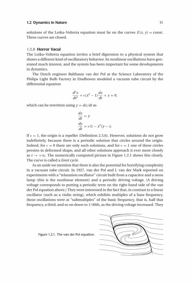
If ε = 1, the origin is a repeller (Definition 2.3.6). However, solutions do not growindefinitely, because there is a periodic solution that circles around the origin.Indeed, for ε = 0 there are only such solutions, and for ε = 1 one of these circlespersists in deformed shape, and all other solutions approach it ever more closelyas t →+∞. The numerically computed picture in Figure 1.2.1 shows this clearly.The curve is called a limit cycle.

As an aside we mention that there is also the potential for horrifying complexityin a vacuum tube circuit. In 1927, van der Pol and J. van der Mark reported onexperiments with a “relaxation oscillator” circuit built from a capacitor and a neonlamp (this is the nonlinear element) and a periodic driving voltage. (A drivingvoltage corresponds to putting a periodic term on the right-hand side of the vander Pol equation above.) They were interested in the fact that, in contrast to a linearoscillator (such as a violin string), which exhibits multiples of a base frequency,these oscillations were at “submultiples” of the basic frequency, that is, half thatfrequency, a third, and so on down to 1/40th, as the driving voltage increased. They

Figure 1.2.1. The van der Pol equation.

12 1. Introduction

obtained these frequencies by listening “with a telephone coupled loosely in someway to the system” and reported that

Often an irregular noise is heard in the telephone receivers before the frequencyjumps to the next lower value. However, this is a subsidiary phenomenon, the maineffect being the regular frequency demultiplication.

This irregular noise was one of the first experimental encounters with what was tobecome known as chaos, but the time was not ripe yet.7

1.2.9 The Other Butterfly Effect8

Population dynamics is naturally done in discrete-time steps when generationsdo not overlap. This was imposed somewhat artificially in the problem posed byLeonardo of Pisa (Section 1.2.2). For many populations this happens naturally,especially insects in temperate zones, including many crop and orchard pests. Apleasant example is a butterfly colony in an isolated location with a fairly constantseasonal cycle (unchanging rules and no external influence). There is no overlap atall between the current generation (this summer) and the next (next summer). Wewould like to know how the size of the population varies from summer to summer.There may be plenty of environmental factors that affect the population, but byassuming unchanging rules we ensure that next summer’s population dependsonly on this summer’s population, and this dependence is the same every year.That means that the only parameter in this model that varies at all is the populationitself. Therefore, up to choosing some fixed constants, the evolution law will specifythe population size next summer as a function of this summer’s population only.The specific evolution law will result from modeling this situation according to ourunderstanding of the biological processes involved.

1. Exponential growth. For instance, it is plausible that a larger population is likelyto lay more eggs and produce a yet larger population next year, proportional, in fact,to the present population. Denoting the present population by x, we then find thatnext year’s population is f (x) = kx for some positive constant k, which is the averagenumber of offspring per butterfly. If we denote the population in year i by xi , wetherefore find that xi+1 = f (xi) = kxi and in particular that x1 = kx0, x2 = kx1 = k2x0,and so on, that is, xi = ki x0; the population grows exponentially. This looks muchlike the exponential–growth problem as we analyzed it in continuous time.

2. Competition. A problem familiar from public debate is sustainability, and theexponential growth model leads to large populations relatively rapidly. It is morerealistic to take into account that a large population will run into problems withlimited food supplies. This will, by way of malnutrition or starvation, reduce the

7 B. van der Pol, J. van der Mark, Frequency demultiplication, Nature 120 (1927), 363–364.8 This is a reference to the statement of Edward Lorenz (see Section 13.3) that a butterfly may flutter

by in Rio and thereby cause a typhoon in Tokyo a week later. Or maybe to butterfly ballots in the2000 Florida election?

1.2 Dynamics in Nature 13

number of butterflies available for egg-laying when the time comes. A relativelysmall number of butterflies next year is the result.

The simplest rule that incorporates such more sensible qualitative propertiesis given by the formula f (x) = k(1− αx)x, where x is the present number ofbutterflies. This rule is the simplest because we have only adduced a linearcorrection to the growth rate k. In this correction α represents the rate at whichfertility is reduced through competition. Alternatively, one can say that 1/α is themaximal possible number of butterflies; that is, if there are 1/α butterflies this year,then they will eat up all available food before getting a chance to lay their eggs;hence they will starve and there will be no butterflies next year. Thus, if again xi

denotes the butterfly population in the year i, starting with i = 0, then the evolutionis given by xi+1 = kxi(1− αxi)=: f (xi). This is a deterministic mathematical modelin which every future state (size of the butterfly colony) can be computed fromthis year’s state. One drawback is that populations larger than 1/α appear to givenegative populations the next year, which could be avoided with a model suchas xi+1 = xiek(1−xi ). But tractability makes the simpler model more popular, and itplayed a significant role in disseminating to scientists the important insight thatsimple models can have complicated long-term behaviors.9

One feature reminiscent of the exponential-growth model is that, for popula-tions much smaller than the limit population, growth is indeed essentiallyexponential: If αx � 1, then 1− αx ≈ 1 and thus xi+1 ≈ kxi ; hence xn ≈ knx0 –but only so long as the population stays small. This makes intuitive sense: Thepopulation is too small to suffer from competition for food, as a large populationwould.

Note that we made a slip in the previous paragraph: The sequence xn ≈ knx0

grows exponentially if k > 1. If this is not the case, then the butterfly colonybecomes extinct. An interesting interplay between reproduction rates and thecarrying capacity influences the possibilities here.

3. Change of variable. To simplify the analysis of this system it is convenient tomake a simple change of variable that eliminates the parameter α. We describe itwith some care here, because changing variables is an important tool in dynamics.

Write the evolution law as x′ = kx(1− αx), where x is the population in one yearand x′ the population in the next year. If we rescale our units by writing y = αx,then we must set

y′ = αx′ = αkx(1− αx) = ky(1− y).

In other words, we now iterate the map g(y) = ky(1− y). The relationship betweenthe maps f and g is given by g(y) = h−1( f (h(y))), where h(y) = y/α = x. This canbe read as “go from new variable to old, apply the old map, and then go to the newvariable again.”

9 As its title shows, getting this message across was the aim of an influential article by Robert M. May,Simple Mathematical Models with Very Complicated Dynamics, Nature 261 (1976), 459–467. Thisarticle also established the quadratic model as the one to be studied. A good impression of the effectson various branches of biology is given by James Gleick, Chaos, Making a New Science, Viking Press,New York, 1987, pp. 78ff.

14 1. Introduction

The effect of this change of variable is to normalize the competition factor α to1. Since we never chose specific units to begin with, let’s rename the variables andmaps back to x and f .

4. The logistic equation. We have arrived at a model of this system that isrepresented by iterations of

f (x) = kx(1− x).

This map f is called the logistic map (or logistic family, because there is a pa-rameter), and the equation x′ = kx(1− x) is called the logistic equation. The termlogistic comes from the French logistique, which in turn derived from logement, thelodgment of soldiers. We also refer to this family of maps as the quadratic family. Itwas introduced in 1845 by the Belgian sociologist and mathematician Verhulst.10

From the brief discussion before the preceding subsection it appears that thecase k ≤ 1 results in inevitable extinction. This is indeed the case. For k < 1, this isclear because kx(1− x) < kx, and for k = 1 it is not hard to verify either, althoughthe population decay is not exponential in this case. By contrast, large values ofk should be good for achieving a large population. Or maybe not. The problem isthat too large a population will be succeeded by a less numerous generation. Onewould hope that the population settles to an agreeable size in due time, at whichthere is a balance between fertility and competition.

� Exercise 1.2.6 Prove that the case k = 1 results in extinction.

Note that, unlike in the simpler exponential growth model, we now refrainedfrom writing down an explicit formula for xn in terms of x0. This formula is givenby polynomials of order 2n. Even if one were to manage to write them down for areasonable n, the formulas would not be informative. We will, in due course, be ableto say quite a bit about the behavior of this model. At the moment it makes sense toexplore it a little to see what kind of behavior occurs. Whether the initial size of thepopulation matters, we have not seen yet. But changing the parameter k certainly islikely to make a difference, or so one would hope, because it would be a sad modelindeed that predicts certain extinction all the time. The reasonable range for k isfrom 0 to 4. [For k > 4, it predicts that a population size of 1/2 is followed two yearslater by a negative population, which makes little biological sense. This suggests thata slightly more sophisticated (nonlinear) correction rule would be a good idea.]

5. Experiments. Increasing kshould produce the possibility of a stable population,that is, to allow the species to avoid extinction. So let’s start working out the modelfor some k > 1. A simpleminded choice would be k = 2, halfway between 0 and 4.

� Exercise 1.2.7 Starting with x = 0.01, iterate 2x(1− x) until you discern a clearpattern.

10 Pierre-Francois Verhulst, Recherches mathematiques sur la loi d’accroissement de la population,Nouvelles Memoires de l’Academie Royale des Sciences et Belles-Lettres de Bruxelles 18 (1845), 1–38.

1.2 Dynamics in Nature 15

Starting from a small population, one obtains steady growth and eventually thepopulation levels off at 1/2. This is precisely the behavior one should expect froma decent model. Note that steady states satisfy x = 2x(1− x), of which 0 and 1/2are the only solutions.

� Exercise 1.2.8 Starting with x = 0.01 iterate 1.9x(1− x) and 2.1x(1− x) untilyou discern a clear pattern.

If k is a little less than 2, the phenomenon is rather the same, for k a little biggerit also goes that way, except for slightly overshooting the steady-state population.

� Exercise 1.2.9 Starting with x = 0.01, iterate 3x(1− x) and 2.9x(1− x) until youdiscern a clear pattern.

For k = 3, the ultimate behavior is about the same, but the way the populationsettles down is a little different. There are fairly substantial oscillations of too largeand too small population that die out slowly, whereas for k near 2 there was only ahint of this behavior, and it died down fast. Nevertheless, an ultimate steady statestill prevails.

� Exercise 1.2.10 Starting with x = 0.01, iterate 3.1x(1− x) until you discern aclear pattern.

For k = 3.1, there are oscillations of too large and too small as before. They doget a little smaller, but this time they do not die down all the way. With a simpleprogram one can iterate this for quite a while and see that no steady state is attained.

� Exercise 1.2.11 Starting with x = 0.66, iterate 3.1x(1− x) until you discern aclear pattern.

In the previous experiment, there is the possibility that the oscillations die downso slowly that the numerics fail to notice. Therefore, as a control, we start the sameiteration at the average of the two values. This should settle down if our diagnosisis correct. But it does not. We see oscillations that grow until their size is as it wasbefore.

These oscillations are stable! This is our first population model that displayspersistent behavior that is not monotonic. No matter at which size you start, thespecies with fertility 3.1 is just a little too fertile for its own good and keeps runninginto overpopulation every other year. Not by much, but forever.

Judging from the previous increments of k there seems only about k = 4 left,but to be safe let’s first try something closer to 3 first. At least it is interesting to seewhether these oscillations get bigger with increasing k. They should. And how big?

� Exercise 1.2.12 Starting with x = 0.66, iterate 3.45x(1− x) and 3.5x(1− x) untilyou discern a clear pattern.

16 1. Introduction

The behavior is becoming more complicated around k = 3.45. Instead of thesimple oscillation between two values, there is now a secondary dance around eachof these values. The oscillations now involve four population sizes: “Big, small, big,Small” repeated in a 4-cycle. The period of oscillation has doubled.

� Exercise 1.2.13 Experiment in a manner as before with parameters slightlylarger than 3.5.

A good numerical experimenter will see some pattern here for a while: Aftera rather slight parameter increase the period doubles again; there are now eightpopulation sizes through which the model cycles relentlessly. A much more minuteincrement brings us to period 16, and it keeps getting more complicated by powersof two. This cascade of period doublings is complementary to what one sees in alinear oscillator such as a violin string or the column of air in wind instruments ororgan pipes: There it is the frequency that has higher harmonics of double, triple,and quadruple the base frequency. Here the frequency is halved successively togive subharmonics, an inherently nonlinear phenomenon.

Does this period doubling continue until k = 4?

� Exercise 1.2.14 Starting with x = .5, iterate 3.83x(1− x) until you discern a clearpattern.

When we look into k = 3.83 we find something rather different: There is aperiodic pattern again, which we seem to have gotten used to. But the period is 3,not a power of 2. So this pattern appeared in an entirely different way. And we don’tsee the powers of 2, so these must have run their course somewhat earlier.

� Exercise 1.2.15 Try k = 3.828.

No obvious pattern here.

� Exercise 1.2.16 Try k = 4.

There is not much tranquility here either.

6. Outlook. In trying out a few parameter values in the simplest possible nonlinearpopulation model we have encountered behavior that differs widely for differentparameter values. Where the behavior is somewhat straightforward we do not havethe means to explain how it evolves to such patterns: Why do periods double fora while? Where did the period-3 oscillation come from? And at the end, and inexperiments with countless other values of the parameter you may choose to try,we see behavior we cannot even describe effectively for lack of words. At this stagethere is little more we can say than that in those cases the numbers are all over theplace.

We return to this model later (Section 2.5, Section 7.1.2, Section 7.4.3 andChapter 11) to explain some of the basic mechanisms that cause these diverse

1.2 Dynamics in Nature 17

behaviors in the quadratic family fk(x) = kx(1− x). We do not provide an exhaus-tive analysis that covers all parameter values, but the dynamics of these maps isquite well understood. In this book we develop important concepts that are neededto describe the complex types of behavior one can see in this situation, and in manyother important ones.

Already this purely numerical exploration carries several lessons. The first oneis that simple systems can exhibit complex long-term behavior. Again, we arrived atthis example from the linear one by making the most benign change possible. Andimmediately we ran into behavior so complex as to defy description. Thereforesuch complex behavior is likely to be rather more common than one would havethought.

The other lesson is that it is worth learning about ways of understanding,describing, and explaining such rich and complicated behavior. Indeed, the impor-tant insights we introduce in this book are centered on the study of systems whereexplicit computation is not feasible or useful. We see that even in the absence ofperfectly calculated results for all time one can make precise and useful qualitativeand quantitative statements about such dynamical systems. Part of the work is todevelop concepts adequate for a description of phenomena of such complexityas we have begun to glimpse in this example. Our study of this particular examplebegins in Section 2.5, where we study the simple behaviors that occur for small pa-rameter values. In Section 7.1.2 and Section 7.4.3 we look at large parameter values.For these the asymptotic behavior is most chaotic. In Chapter 11 we present someof the ideas used in understanding the intermediate parameter regime, where thetransitions to maximal complexity occur.

As an interesting footnote we mention that the analogous population withcontinuous time (which is quite reasonable for other species) has none of thiscomplexity (see Section 2.4.2).

1.2.10 A Flash of InspirationAs another example of dynamics in nature we can take the flashing of fireflies.Possibly the earliest report of a remarkable phenomenon is from Sir Francis Drake’s1577 expedition:

[o]ur general . . . sailed to a certaine little island to the southwards of Celebes, . . .throughly growen with wood of a large and high growth. . . .Among these trees nightby night, through the whole land, did shew themselves an infinite swarme of fierywormes flying in the ayre, whose bodies beeing no bigger than our common Englishflies, make such a shew of light, as if every twigge or tree had been a burning candle.11

A clearer description of what is so remarkable about these fireflies was given byEngelbert Kampfer, a doctor from eastern Westphalia who made a 10-year voyagethrough Russia, Persia, southeast Asia, and Japan. On July 6, 1690, he traveled downthe Chao Phraya (Meinam) River from Bangkok and observed:

The glowworms (Cicindelae) represent another shew, which settle on some trees,like a fiery cloud, with this surprising circumstance, that a whole swarm of these

11 Richard Hakluyt (pronounced Hack-loot), A Selection of the Principal Voyages, Traffiques andDiscoveries of the English Nation, edited by Laurence Irving, Knopf, New York, 1926.